![SOLUCIONES TEMA 2 Ejercicio 1 - UC3Mmlazaro/Docencia/GISC_GIT-CD/MD... · 6 4 c[0] c[1] c[2] c[3] 3 7 7 5= 2 6 6 4 0 1 0 0 3 7 7 5; P = 2 6 6 4 1=2 0 1 1=2 1=2 1 0 1=2 3 7 7 5 Resolviendo](https://static.fdocument.org/doc/165x107/5f0e38827e708231d43e3113/soluciones-tema-2-ejercicio-1-mlazarodocenciagiscgit-cdmd-6-4-c0-c1.jpg)


γλώσσες
Σελίδες
Νομικός

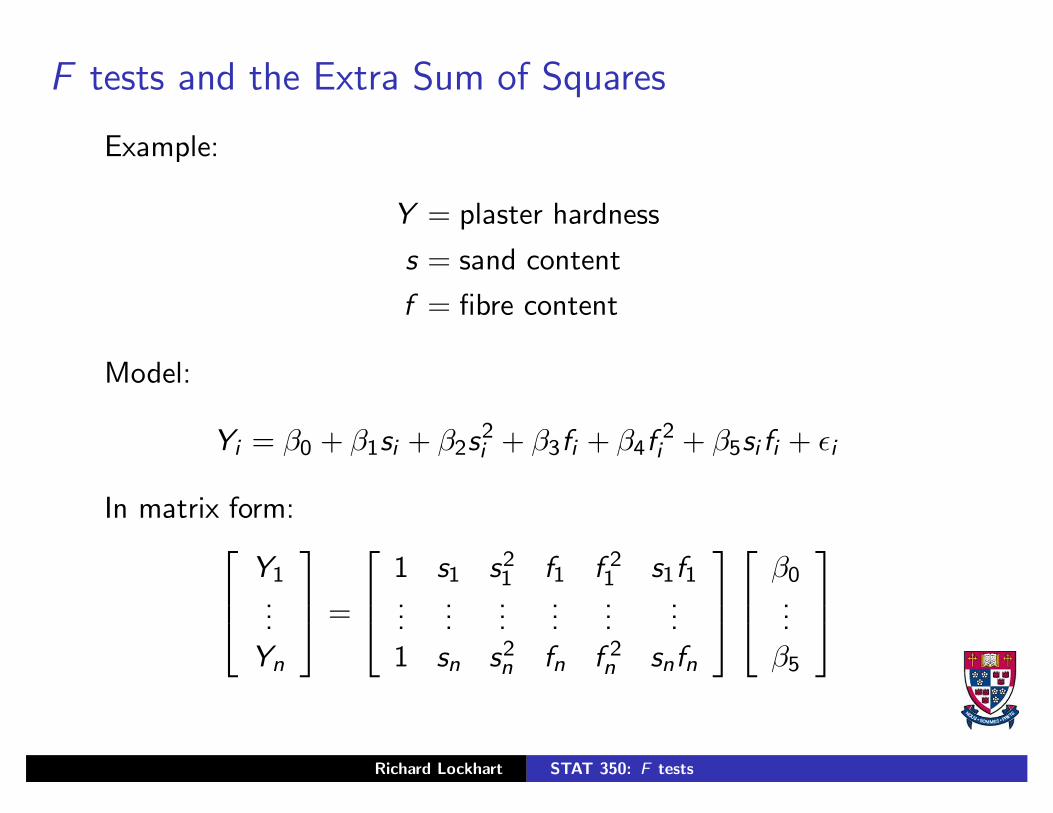
F tests and the Extra Sum of Squares
Example:
Y = plaster hardness
s = sand content
f = fibre content
Model:
Yi = β0 + β1si + β2s2i + β3fi + β4f
2i + β5si fi + ǫi
In matrix form: Y1...
Yn
=
1 s1 s21 f1 f 2
1 s1f1...
......
......
...1 sn s2
n fn f 2n snfn
β0
...β5
Richard Lockhart STAT 350: F tests

Hypotheses to test
Questions:
◮ Do we need the S ∗ F term?
◮ Do we need the F or F 2 terms?
◮ Do we need the S or S2 terms?
To answer these questions we test
◮ Ho : β5 = 0
◮ Ho : β3 = β4 = 0 (or perhaps Ho : β3 = β4 = β5 = 0)
◮ Ho : β1 = β2 = 0
Richard Lockhart STAT 350: F tests
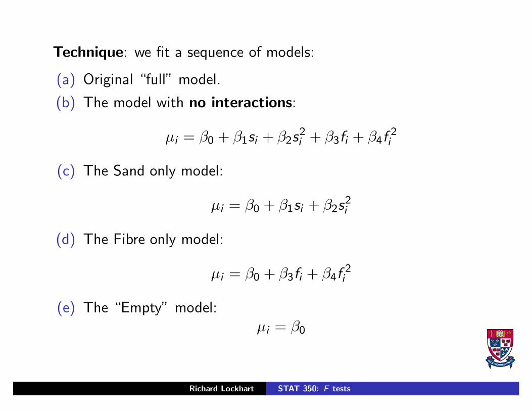
Technique: we fit a sequence of models:
(a) Original “full” model.
(b) The model with no interactions:
µi = β0 + β1si + β2s2i + β3fi + β4f
2i
(c) The Sand only model:
µi = β0 + β1si + β2s2i
(d) The Fibre only model:
µi = β0 + β3fi + β4f2i
(e) The “Empty” model:µi = β0
Richard Lockhart STAT 350: F tests

Each model has design matrix which is submatrix of full designmatrix:
Y = [1|X1|X2|X3]
β0
β1
β2
β3
β4
β5
+ ǫ
The design matrices for the models a, b, c, d and e are given by
Xa = X
Xb = [1|X1|X2]
Xc = [1|X1]
Xd = [1|X2]
Xe = [1]
Note that 1 is a column vector of n 1s.
Richard Lockhart STAT 350: F tests
F tests
◮ Can compare two models easily if one is a special case of theother.
◮ Example: design matrix of first model is submatrix of secondobtained by selecting subcolumns.
◮ Model (b) is a special case of (a), model (c) is a special caseof (a) or (b) but models (c) and (d) are not comparable.
Richard Lockhart STAT 350: F tests
Comparing two models: General Theory
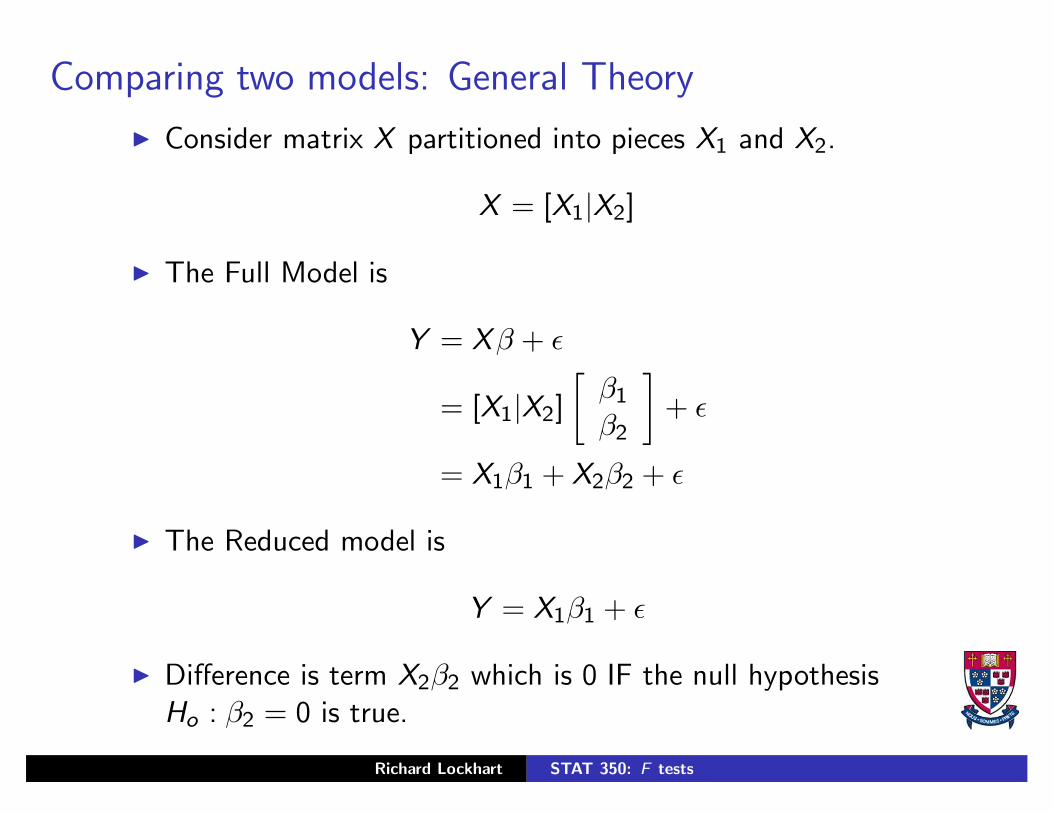
◮ Consider matrix X partitioned into pieces X1 and X2.
X = [X1|X2]
◮ The Full Model is
Y = Xβ + ǫ
= [X1|X2]
[β1
β2
]+ ǫ
= X1β1 + X2β2 + ǫ
◮ The Reduced model is
Y = X1β1 + ǫ
◮ Difference is term X2β2 which is 0 IF the null hypothesisHo : β2 = 0 is true.
Richard Lockhart STAT 350: F tests
Dimensions
◮ β has p parameters.
◮ βi has pi parameters with p1 + p2 = p.
Richard Lockhart STAT 350: F tests
Testing Ho : β2 = 0
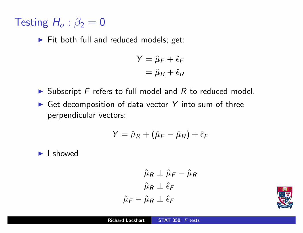
◮ Fit both full and reduced models; get:
Y = µ̂F + ǫ̂F
= µ̂R + ǫ̂R
◮ Subscript F refers to full model and R to reduced model.
◮ Get decomposition of data vector Y into sum of threeperpendicular vectors:
Y = µ̂R + (µ̂F − µ̂R) + ǫ̂F
◮ I showed
µ̂R ⊥ µ̂F − µ̂R
µ̂R ⊥ ǫ̂F
µ̂F − µ̂R ⊥ ǫ̂F
Richard Lockhart STAT 350: F tests
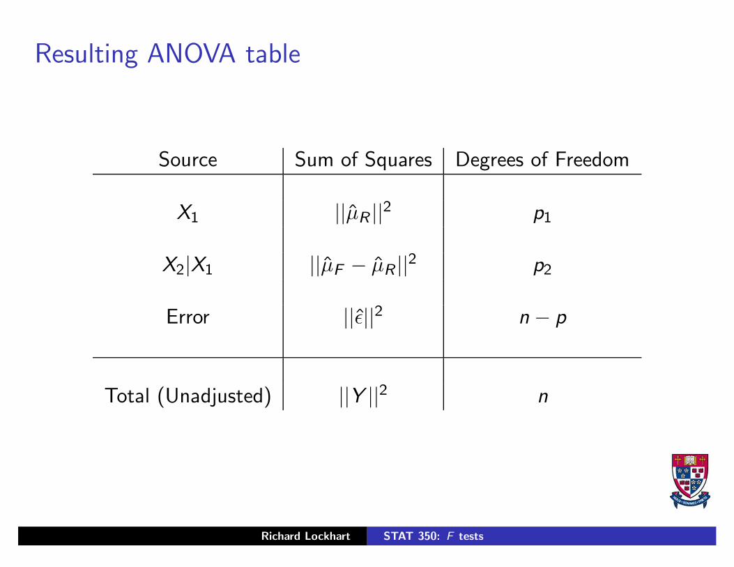
Resulting ANOVA table
Source Sum of Squares Degrees of Freedom
X1 ||µ̂R ||2 p1
X2|X1 ||µ̂F − µ̂R ||2 p2
Error ||ǫ̂||2 n − p
Total (Unadjusted) ||Y ||2 n
Richard Lockhart STAT 350: F tests

F tests again
◮ In this table the notation X2|X1 means X2 adjusted for X1 orX2 after fitting X1.
◮ This table can now be used to test Ho : β2 = 0 by computing
F =MS(X2|X1)
MSE=||µ̂F − µ̂R ||2/p2
||ǫ̂||2/(n − p)
◮ Get P value from Fp2,n−p distribution.
◮ P value usually computed by software.
◮ Do level α test by comparing P to α.
Richard Lockhart STAT 350: F tests
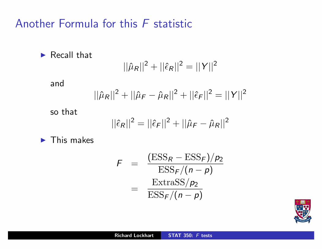
Another Formula for this F statistic
◮ Recall that||µ̂R ||2 + ||ǫ̂R ||2 = ||Y ||2
and||µ̂R ||2 + ||µ̂F − µ̂R ||2 + ||ǫ̂F ||2 = ||Y ||2
so that||ǫ̂R ||2 = ||ǫ̂F ||2 + ||µ̂F − µ̂R ||2
◮ This makes
F =(ESSR − ESSF )/p2
ESSF/(n − p)
=ExtraSS/p2
ESSF/(n − p)
Richard Lockhart STAT 350: F tests
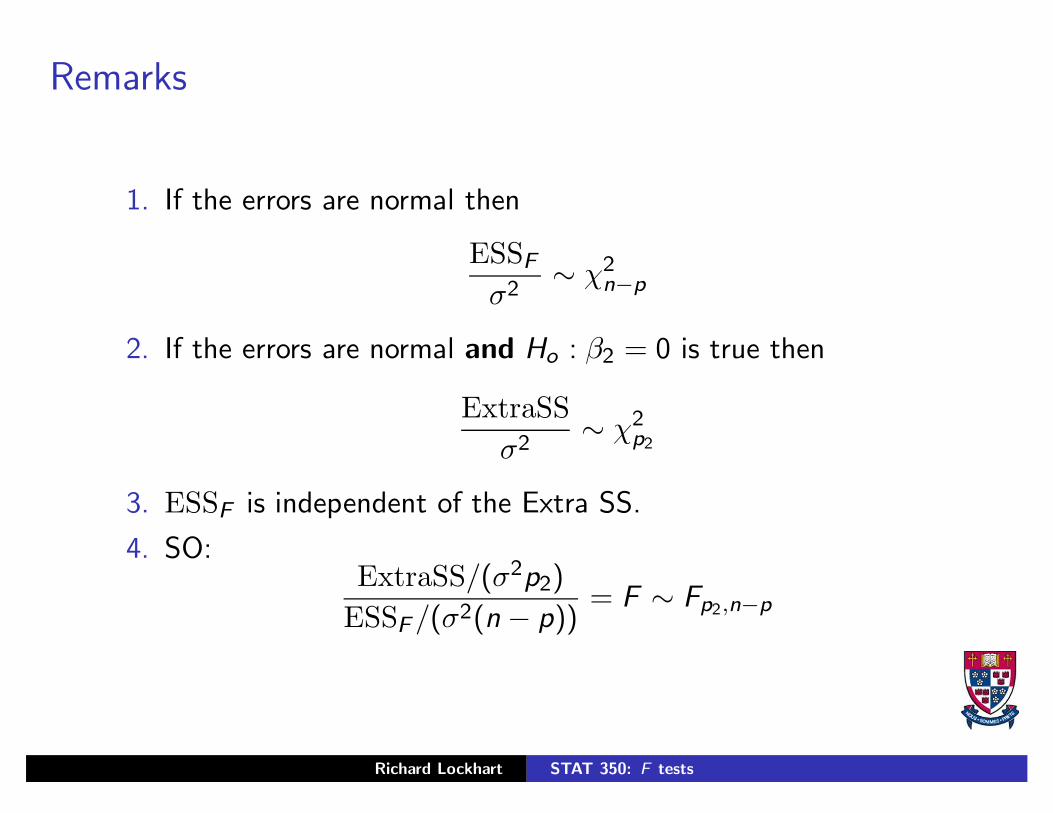
Remarks
1. If the errors are normal then
ESSF
σ2∼ χ2
n−p
2. If the errors are normal and Ho : β2 = 0 is true then
ExtraSSσ2
∼ χ2p2
3. ESSF is independent of the Extra SS.
4. SO:ExtraSS/(σ2p2)
ESSF /(σ2(n − p))= F ∼ Fp2,n−p
Richard Lockhart STAT 350: F tests
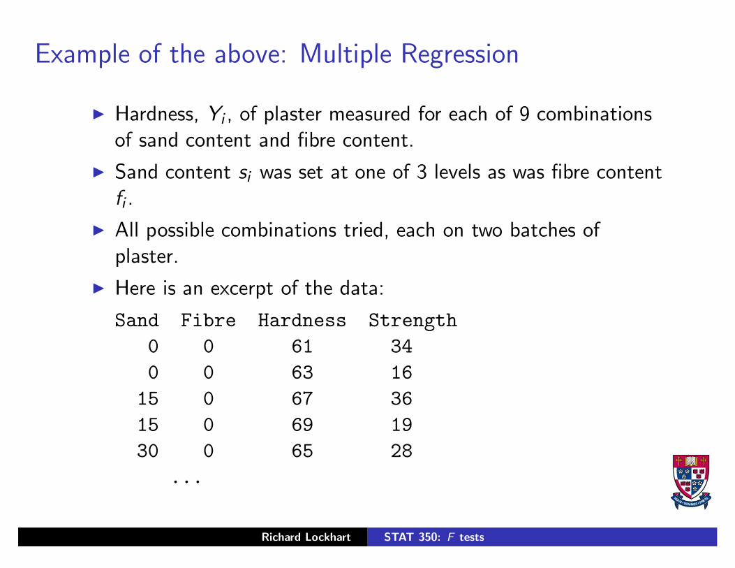
Example of the above: Multiple Regression
◮ Hardness, Yi , of plaster measured for each of 9 combinationsof sand content and fibre content.
◮ Sand content si was set at one of 3 levels as was fibre contentfi .
◮ All possible combinations tried, each on two batches ofplaster.
◮ Here is an excerpt of the data:
Sand Fibre Hardness Strength0 0 61 340 0 63 16
15 0 67 3615 0 69 1930 0 65 28
...
Richard Lockhart STAT 350: F tests
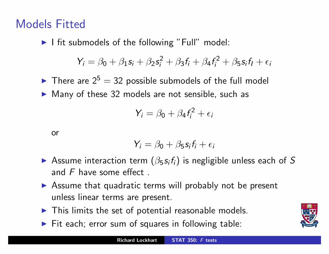
Models Fitted
◮ I fit submodels of the following ”Full” model:
Yi = β0 + β1si + β2s2i + β3fi + β4f
2i + β5si fI + ǫi
◮ There are 25 = 32 possible submodels of the full model
◮ Many of these 32 models are not sensible, such as
Yi = β0 + β4f2i + ǫi
orYi = β0 + β5si fi + ǫi
◮ Assume interaction term (β5si fi) is negligible unless each of Sand F have some effect .
◮ Assume that quadratic terms will probably not be presentunless linear terms are present.
◮ This limits the set of potential reasonable models.
◮ Fit each; error sum of squares in following table:
Richard Lockhart STAT 350: F tests
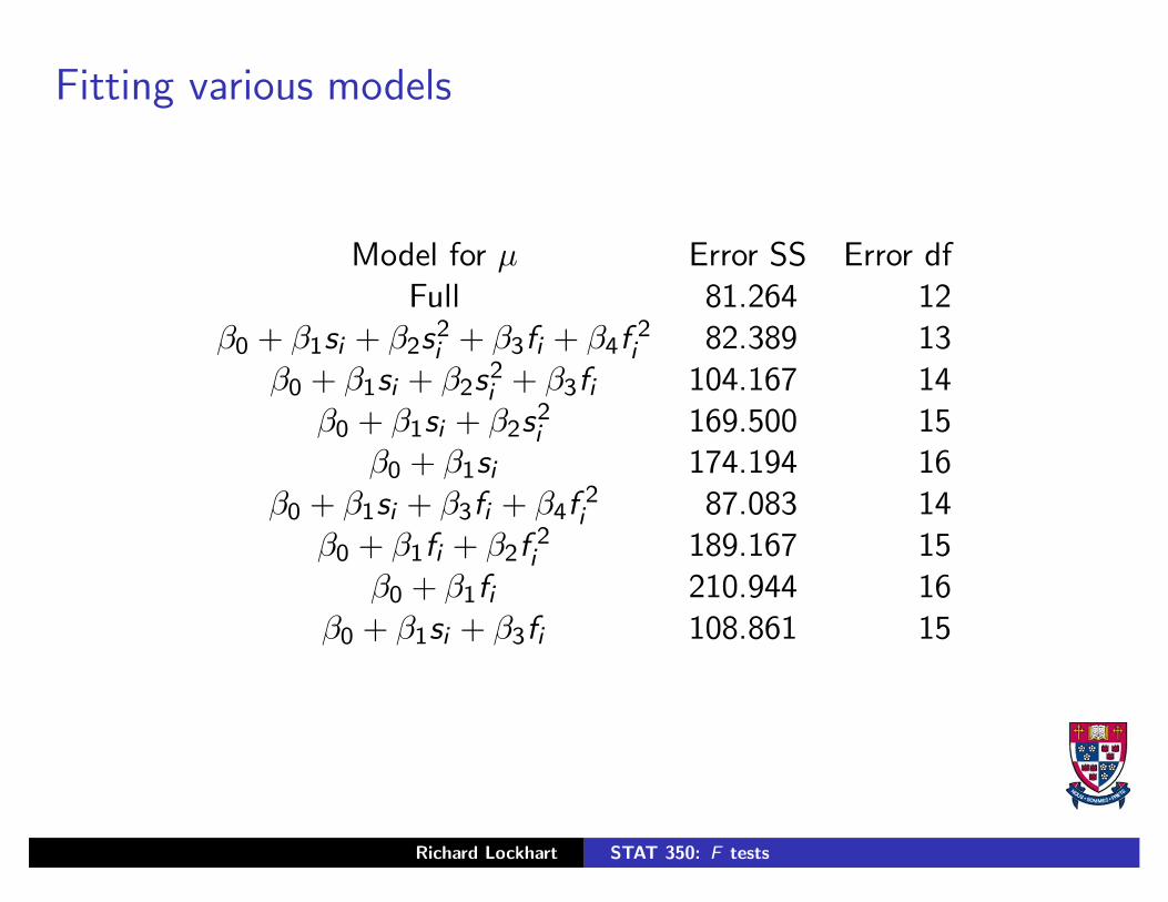
Fitting various models
Model for µ Error SS Error dfFull 81.264 12
β0 + β1si + β2s2i + β3fi + β4f
2i 82.389 13
β0 + β1si + β2s2i + β3fi 104.167 14
β0 + β1si + β2s2i 169.500 15
β0 + β1si 174.194 16β0 + β1si + β3fi + β4f
2i 87.083 14
β0 + β1fi + β2f2i 189.167 15
β0 + β1fi 210.944 16β0 + β1si + β3fi 108.861 15
Richard Lockhart STAT 350: F tests
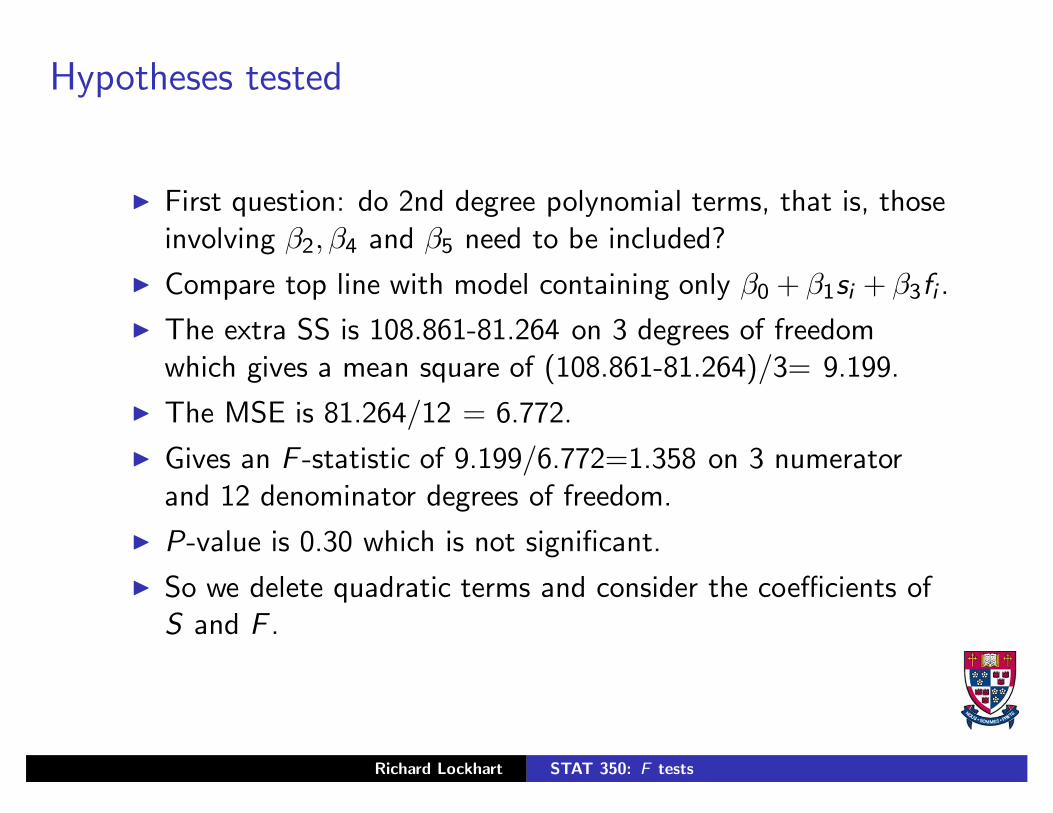
Hypotheses tested
◮ First question: do 2nd degree polynomial terms, that is, thoseinvolving β2, β4 and β5 need to be included?
◮ Compare top line with model containing only β0 + β1si + β3fi .
◮ The extra SS is 108.861-81.264 on 3 degrees of freedomwhich gives a mean square of (108.861-81.264)/3= 9.199.
◮ The MSE is 81.264/12 = 6.772.
◮ Gives an F -statistic of 9.199/6.772=1.358 on 3 numeratorand 12 denominator degrees of freedom.
◮ P-value is 0.30 which is not significant.
◮ So we delete quadratic terms and consider the coefficients ofS and F .
Richard Lockhart STAT 350: F tests
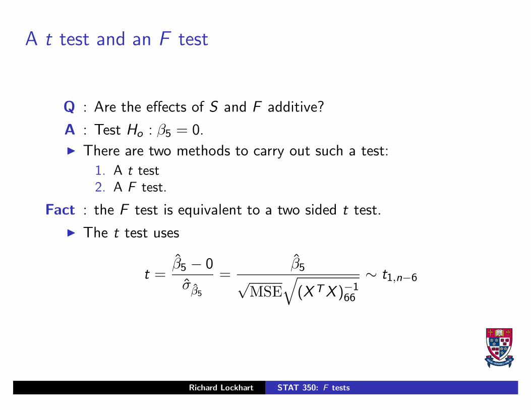
A t test and an F test
Q : Are the effects of S and F additive?
A : Test Ho : β5 = 0.
◮ There are two methods to carry out such a test:
1. A t test2. A F test.
Fact : the F test is equivalent to a two sided t test.
◮ The t test uses
t =β̂5 − 0
σ̂β̂5
=β̂5√
MSE√
(XT X )−166
∼ t1,n−6
Richard Lockhart STAT 350: F tests
t tests
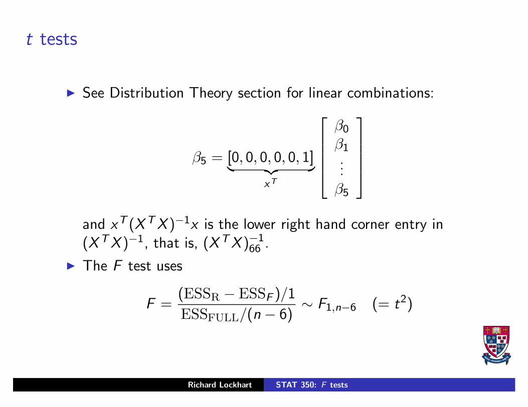
◮ See Distribution Theory section for linear combinations:
β5 = [0, 0, 0, 0, 0, 1]︸ ︷︷ ︸xT
β0
β1...
β5
and xT (XT X )−1x is the lower right hand corner entry in(XTX )−1, that is, (XTX )−1
66 .
◮ The F test uses
F =(ESSR − ESSF )/1
ESSFULL/(n − 6)∼ F1,n−6 (= t2)
Richard Lockhart STAT 350: F tests

Testing for Main Effects
The Data
◮ Y = hardness of plaster. n = 18 batches.
◮ S = sand content. Values used 0%, 15% 30%.
◮ F = fibre content. Values used 0%, 25% 50%.
◮ Factorial design with 2 replicates.
Richard Lockhart STAT 350: F tests
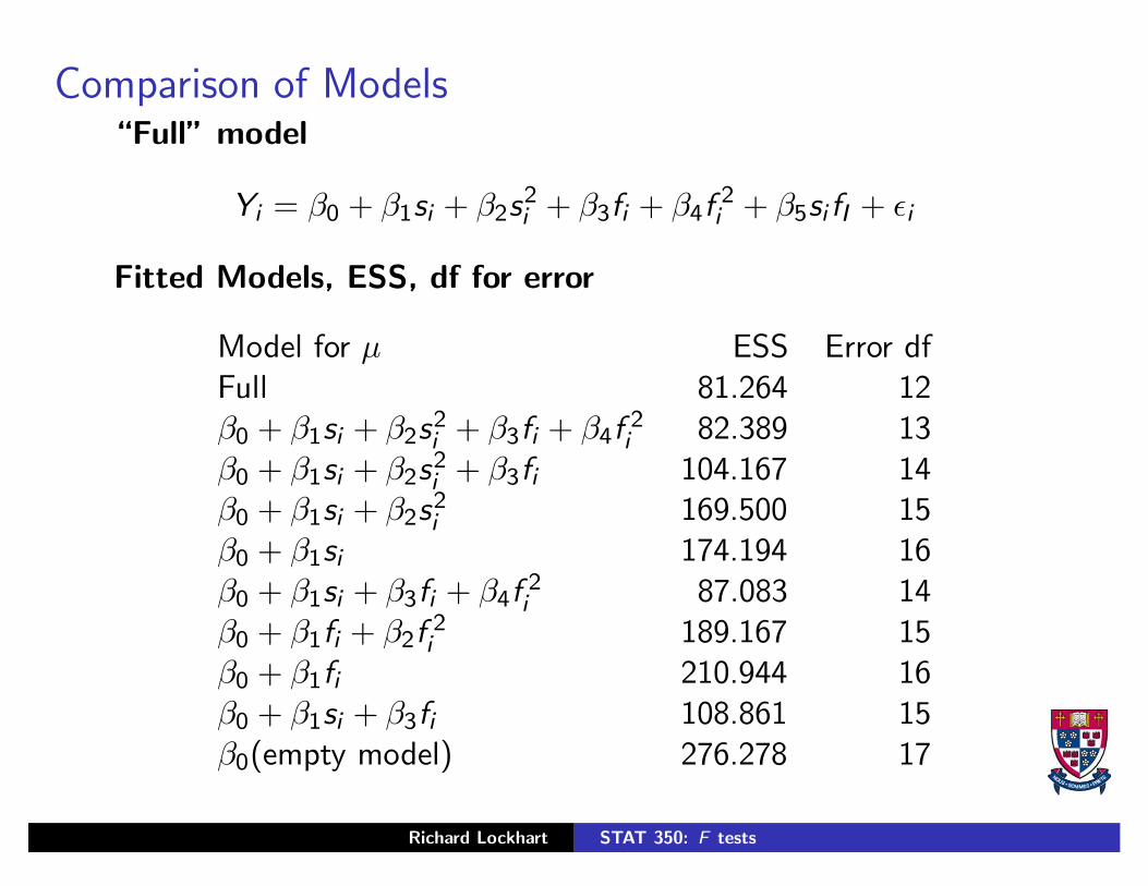
Comparison of Models“Full” model
Yi = β0 + β1si + β2s2i + β3fi + β4f
2i + β5si fI + ǫi
Fitted Models, ESS, df for error
Model for µ ESS Error dfFull 81.264 12β0 + β1si + β2s
2i + β3fi + β4f
2i 82.389 13
β0 + β1si + β2s2i + β3fi 104.167 14
β0 + β1si + β2s2i 169.500 15
β0 + β1si 174.194 16β0 + β1si + β3fi + β4f
2i 87.083 14
β0 + β1fi + β2f2i 189.167 15
β0 + β1fi 210.944 16β0 + β1si + β3fi 108.861 15β0(empty model) 276.278 17
Richard Lockhart STAT 350: F tests
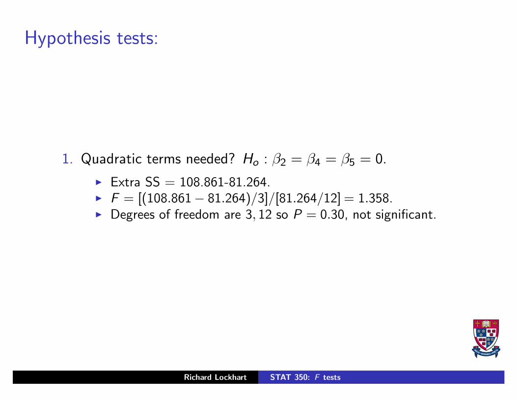
Hypothesis tests:
1. Quadratic terms needed? Ho : β2 = β4 = β5 = 0.
◮ Extra SS = 108.861-81.264.◮ F = [(108.861− 81.264)/3]/[81.264/12] = 1.358.◮ Degrees of freedom are 3, 12 so P = 0.30, not significant.
Richard Lockhart STAT 350: F tests
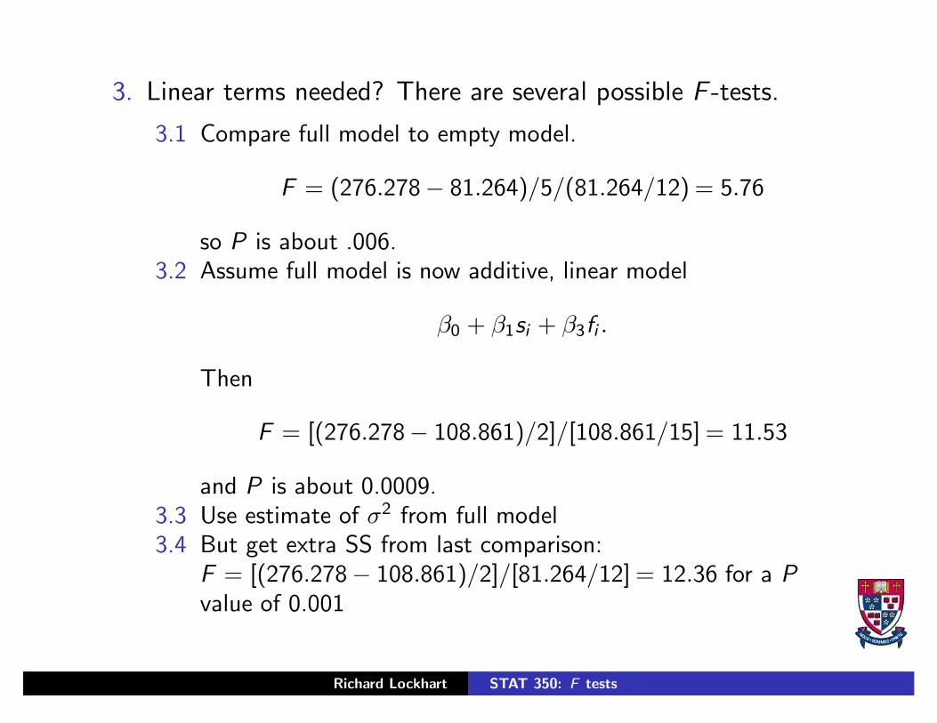
3. Linear terms needed? There are several possible F -tests.
3.1 Compare full model to empty model.
F = (276.278− 81.264)/5/(81.264/12) = 5.76
so P is about .006.3.2 Assume full model is now additive, linear model
β0 + β1si + β3fi .
Then
F = [(276.278− 108.861)/2]/[108.861/15] = 11.53
and P is about 0.0009.3.3 Use estimate of σ2 from full model3.4 But get extra SS from last comparison:
F = [(276.278− 108.861)/2]/[81.264/12] = 12.36 for a Pvalue of 0.001
Richard Lockhart STAT 350: F tests
Conclusions
◮ Both Sand and Fibre influence Hardness.
◮ Linear terms in S and F are adequate.
Richard Lockhart STAT 350: F tests
Top Related