2.2. Cauchy problem for quasilinear PDE 19

P0. Then the integral surface containing Γ1 (which exists by the local existence theorem asJΓ1 (P0) = 0) also contains a part of Γ containing P0, since Γ is a characteristic curve throughP0.

Then there are infinitely many solutions to the Characteristic Cauchy problem cor-responding to infinitely many ways of choosing Γ1, a proof of this is left as an exercise tothe reader.

Proof of (2): Lemma 2.20 asserts that Γ must be a characteristic curve if there is asolution to the Cauchy problem when J (s) ≡ 0 for all s ∈ I . Thus JΓ ≡ 0 and Γ does nothave a characteristic direction anywhere are incompatible if the Cauchy problem admitsa differentiable solution. Thus we conclude that the Cauchy problem does not admit asolution. This completes the proof of (2).

Remark 2.22. In the previous lemma, we discussed the case of J ≡ 0. It will be interestingto know what happens when J vanishes but does not vanish identically. In view of thelast two results, we understand the situation completely whenever J is not equal to zero,or stretches where J is identically equal to zero. If Γ is not a characteristic curve, thenwe expect integral surfaces to have singularities near the points where J vanishes. SeeExercise 2.10.

Remark 2.23 (On the three examples of Subsection 2.2.2). Let us return to the threeexamples that we considered in Subsection 2.2.2. We have the following observationsregarding them.

(i) In Example 2.12, Jacobian is non-zero and hence we have a unique solution. In otherwords, the transversality condition is satisfied. Geometrically, this means that thetangential directions for the two intersecting curves, namely, the base characteristiccorresponding to the characteristic curve passing through a point P , and the projec-tion of the initial curve Γ , are not parallel at any point.

(ii) In Example 2.13, J ≡ 0 and the initial curve is a characteristic curve and hence ithas infinitely many solutions. In other words, the transversality condition is notsatisfied. That is, the tangential directions for the two intersecting curves, namely,the base characteristics corresponding to the characteristic curve passing through apoint P , and the projection of the initial curve Γ are parallel at any point P . How-ever in this example, the initial curve is a characteristic. That is, the characteris-tic direction coincides with the tangential direction for initial curve, and thus byLemma 2.21 guaranteed the existence of an infinite number of solutions.

(iii) In Example 2.14, J ≡ 0 and the initial curve is not a characteristic curve and henceit has no solutions. Even though the situation is similar to that of Example 2.13(namely, transversality condition is not satisfied), in this example we do not havesolutions. The reason for non-existence of solutions is that the initial curve is not acharacteristic.

Some more terminology

(i) Characteristic direction (a, b , c) is also called Monge’s direction.(ii) Characteristic equation is also called Monge’s equation.

(iii) Characteristic curves are also called Monge’s curves.

2.2.4 Burgers equation

Let us solve the Cauchy problem for Burgers’ equation.

October 27, 2015 Sivaji

20 Chapter 2. First order PDE

Example 2.24 (Burgers’ equation).Cauchy Problem to be solved is

uy + u ux = 0, u(x, 0) = h(x) for x ∈R, y > 0. (2.47)

This is a Cauchy problem for a first order quasilinear PDE.

Parametrization of the initial curve Γ

Γ : x = s , y = 0, z = h(s), s ∈R. (2.48)

Characteristic equations and the initial conditions for solving them

d xd t= z,

d yd t= 1,

d zd t= 0, (2.49)

with initial conditionsx(0) = s , y(0) = 0, z(0) = h(s). (2.50)

The characteristic equations is a system of linear ODE and hence the IVP has a uniquesolution defined for all t ∈R.

Solutions of the IVP for Characteristic equationsThe unique solution to (2.49)-(2.50) is given by

x =X (s , t ) = h(s)t + s , y = Y (s , t ) = t , z = Z(s , t ) = h(s) defined for (s , t ) ∈R×R.(2.51)

Note that z = h(s) means that solution u(x, y) ≡ h(s ) on the base characteristic curvegiven by x =X (s , t ) = h(s )t + s , y = Y (s , t ) = t , which is a straight line passing through(s , 0) on the x-axis.

Comment on the Base characteristicsProjection of a characteristic curve (corresponds to a fixed s ) to the xy-plane are given

by parametric equations(h(s)t + s , t ) : t ∈R (2.52)

In cartesian coordinates, the equation is given by

X = h(s)Y + s . (2.53)

This is a straight line with slope1

h(s). Base characteristics corresponding to different

s1 and s2 meet if and only if the following system has a solution1 −h(s1)1 −h(s2)

X0Y0

=

s1s2

(2.54)

Since s1 = s2, even if h(s1) = h(s2) the corresponding base characteristics are two parallellines and hence do not intersect. If h(s1)− h(s2) = 0, then both straight lines meet at aunique point given by

X0Y0

=

1h(s1)− h(s2)

s2h(s1)− s1h(s2)

s2− s1

(2.55)

Sivaji IIT Bombay

2.2. Cauchy problem for quasilinear PDE 21

Comments on Jacobian and explain if the local existence and uniqueness theoremcan be applied or if it is a characteristic Cauchy problem

J =∂ (X ,Y )∂ (s , t )

= h ′(s )t + 1 h(s)

0 1

= 1+ h ′(s )t . (2.56)

We expect something wrong at (s , t )where 1+h ′(s)t = 0, i.e., at t =− 1h ′(s ) . We will come

back to this later on. Nevertheless,

J =∂ (X ,Y )∂ (s , t )

|(s ,t )=(s0,0) = 1 h(s0)

0 1

= 0. (2.57)

Thus we can apply the local existence theorem (Theorem 2.17) and we get a unique solu-tion to the Cauchy problem near (s0, 0, h(s0)) ∈ Γ .The Final solution(s)

Eliminating s , t , we get

z = Z(S(x, y),T (x, y)) = h(x − y z) (2.58)

Thus the solution to Cauchy problem is given implicitly by

u = h(x − y u). (2.59)

Propagation of monotonic initial profiles

We consider three examples of Cauchy problems for Burgers’ equation, wherein Cauchydata comprise of a monotonic function that is also piecewise linear. Since piecewise linearfunctions need not be differentiable, they do not satisfy the hypothesis of the existenceand uniqueness theorem, namely Theorem 2.17.

However, explicit ‘solution’ of the Cauchy problem can be obtained using the implicitformula (2.59), which exhibit the effects of nonlinear nature of Burgers’ equation, andthe monotonicity of cauchy data (and not due to piecewise linearity of the Cauchy data).Thus these examples highlight the role played by nonlinearity of a PDE in the solutions ofCauchy problems. On the other hand, Cauchy data can be discontinuous in applicationssuch as study of traffic near a traffic signal.

In the first example, the method of characterisitcs fails to determine a solution in someregion of the upper half-plane. This is due to the discontinuity in the piecewise constant,non-decreasing Cauchy data.

Example 2.25 (Characteristics do not reach some points). Consider Burgers equationwith Cauchy data given by

h(x) = −1 if x < 0,

1 if x ≥ 0.(2.60)

Equation for the family of base characteristics (indexed by s ∈R) is given by

y =1

h(s )x − s

h(s).

October 27, 2015 Sivaji

22 Chapter 2. First order PDE

..

x =y

.

x =−y

.

u(x, y) =−1

.

u(x, y) = 1

.

No characteristics.

.

Solution is undetermined.

.−4

.−3

.−2

.−1

.0.

1.

2.

3.

4

Figure 2.1. Example 2.25: characterisitcs and the solution

Thus a base characteristic passing through a point (s , 0) with s < 0 is given by the liney =−x+ s , which is a family of lines parallel to y =−x. The solution u =−1 along eachof these straight lines, since the solution is constant along each of the base characterisitcsby (2.51). Similarly, for s ≥ 0 the base characteristic passing through a point (s , 0) isgiven by the line y = x − s , which is a family of lines parallel to y = x. The solutionu = 1 along each of these straight lines. However, no characteristic passes through theV -shaped region in the upper half-plane which is bounded by the lines y = x and y =−xas illustrated in Figure 2.1.

We may interpret by saying that base characterisitcs carry information from Cauchydata (presecribed on x-axis in this case) into rest of the upper half-plane. Since there areno base characterisitcs passing through the V -shaped region, we may say that informationfrom the Cauchy data does not reach this region. Thus a solution to this Cauchy problemcould be determined in the complement of the V -shaped region. In Section 2.3, a solutionof the Cauchy problem in the V -shaped region will be obtained, in a generalized sense.Note that if the non-decreasing function h were also continuous, then a base characteristicwould pass through every point of the upper half-plane.

In the next example, solution becomes multi-valued in some region of the upper half-plane. This is due to the nonlinearity of Burgers’ equation, and non-increasing Cauchydata.

Example 2.26 (Intersecting base characteristics). Consider Burgers equation with Cauchydata given by

h(x) =§

1 if x < 0,−1 if x ≥ 0. (2.61)

Equation for the family of base characteristics (indexed by s ∈R) is given by

y =1

h(s)x − s

h(s).

Thus a base characteristic passing through a point (s , 0) with s < 0 is given by the liney = x − s , which is a family of lines parallel to y = x. The solution u = 1 along each of

Sivaji IIT Bombay

2.2. Cauchy problem for quasilinear PDE 23

..

u(x, y) = 1

.

u(x, y) =−1

.

Intersecting characteristics.

.

Solution becomes multi-valued.

.−4

.−3

.−2

.−1

.0.

1.

2.

3.

4

Figure 2.2. Example 2.26: characterisitcs and the solution

these straight lines, since the solution is constant along each of the base characterisitcs by(2.51).

For s ≥ 0 the base characteristic passing through a point (s , 0) is given by the liney =−x+ s , which is a family of lines parallel to y =−x. The solution u =−1 along eachof these straight lines.

However, two base characteristics pass through each point of the V -shaped regionthat is bounded by the lines y = x and y =−x in the upper half-plane: one coming fromthe negative x-axis, and another from positive x-axis (see Figure 2.2). As a consequence,multiplicity of information is reaching this V -shaped region, and they are in conflict (basecharacterisitcs coming from negative, and positive x-axis carry the information u = 1, andu = −1 respectively), and thus solution becomes multi-valued in the V -shaped region,solution. The question is how to make sense of solution at those points? This will bediscussed in Section 2.3.

Example 2.27. Consider Burgers equation with Cauchy data given by

h(x) =

1 if x ≤ 0,

1− x if 0≤ x ≤ 1,0 if x ≥ 1.

(2.62)

In this example, there are three distinct families of base characterisitcs (see Figure 2.3).They are

(i) characterisitcs emanating from negative x-axis (F1 family). These are lines parallelto y = x, and along them u = 1.

(ii) characterisitcs emanating from points (s , 0) where 0 < s < 1 (F2 family). Thisfamily has varied slopes, as s → 1 the slopes increase from 1 (at s = 0) to∞ (ats = 1).

(iii) characterisitcs emanating from points (s , 0)where s ≥ 1 (F3 family). These are linesparallel to x = 1, and along them u = 0.

October 27, 2015 Sivaji

24 Chapter 2. First order PDE

Since slopes of base characterisitcs increase with s ∈ R, some of them would intersect.Since solution is constant along each base characteristic, at points of intersection of twobase characterisitcs on which solution is different, solution becomes multi-valued, andloses its meaning. Since a solution is uniquely determined in regions where base charac-terisitcs do not intersect, we are interested in knowing if the base characterisitcs intersect.

Let γs1and γs2

be two base characteristics emanating from the points (s1, 0) and (s2, 0)respectively, with s1 < s2. Recall that γs1

and γs2are straight lines, and are given by the

equations

γs1: x = h(s1)y + s1,

γs2: x = h(s2)y + s2.

If γs1and γs2

intersect a point (x0, y0), then we have

x0 =h(s1)s2− h(s2)s1

h(s1)− h(s2), y0 =

s2− s1

h(s1)− h(s2). (2.63)

We have the following observations regarding γs1and γs2

.

(i) If s1 < s2 ≤ 0, then γs1and γs2

do not intersect as they are parallel to the line y = x.Thus no two members of the F1 family intersect.

(ii) If s1 ≤ 0< s2 < 1, then γs1and γs2

intersect at

x0 =s2− s1+ s1 s2

s2, y0 =

s2− s1

s2. (2.64)

We are interested in finding out the minimum value of y0 as s1 varies in (−∞, 0],and s2 varies in (0,1). In other words, if y is interpreted as time, we are interested infinding out the first time that some member of the family F1 intersects a memberof the family F2. Minimum value of y0 is obtained when s1 = 0 and s2 is arbitrary,and equals 1. The corresponding value of x0 is then given by x0 = 1. In other words,each γs2

intersects γ0 at the point (1,1), as illustrated in Figure 2.3.

(iii) If s1 ≤ 0 and s2 ≥ 1, then γs1and γs2

intersect at

x0 = s2, y0 = s2− s1. (2.65)

The minimum value of y0 as s1 varies in (−∞, 0], and s2 varies in [1,∞) is the firsttime that some member of the family F1 intersects a member of the family F3, isobtained when s1 = 0 and s2 = 1, and is equal to 1. The corresponding value of x0 isthen given by x0 = 1. In other words, γ1 intersects γ0 at the point (1,1), as illustratedin Figure 2.3.

(iv) If 0< s1 < s2 < 1, then γs1and γs2

intersect at

x0 = 1, y0 = 1. (2.66)

That is, all the characteristics from the family F3 intersect at the point (1,1), asillustrated in Figure 2.3.

(v) If 0< s1 < 1 and s2 ≥ 1, then γs1and γs2

intersect at

x0 = s2, y0 =s2− s1

1− s1. (2.67)

Sivaji IIT Bombay

2.2. Cauchy problem for quasilinear PDE 25

..

y = 1

.

u(x, y) = 1

.

u(x, y) = 0

.

Intersecting characteristics

.

Solution becomes multi-valued

.u = 1−x

1−y.−4

.−3

.−2

.−1

.0.

1.

2.

3.

4

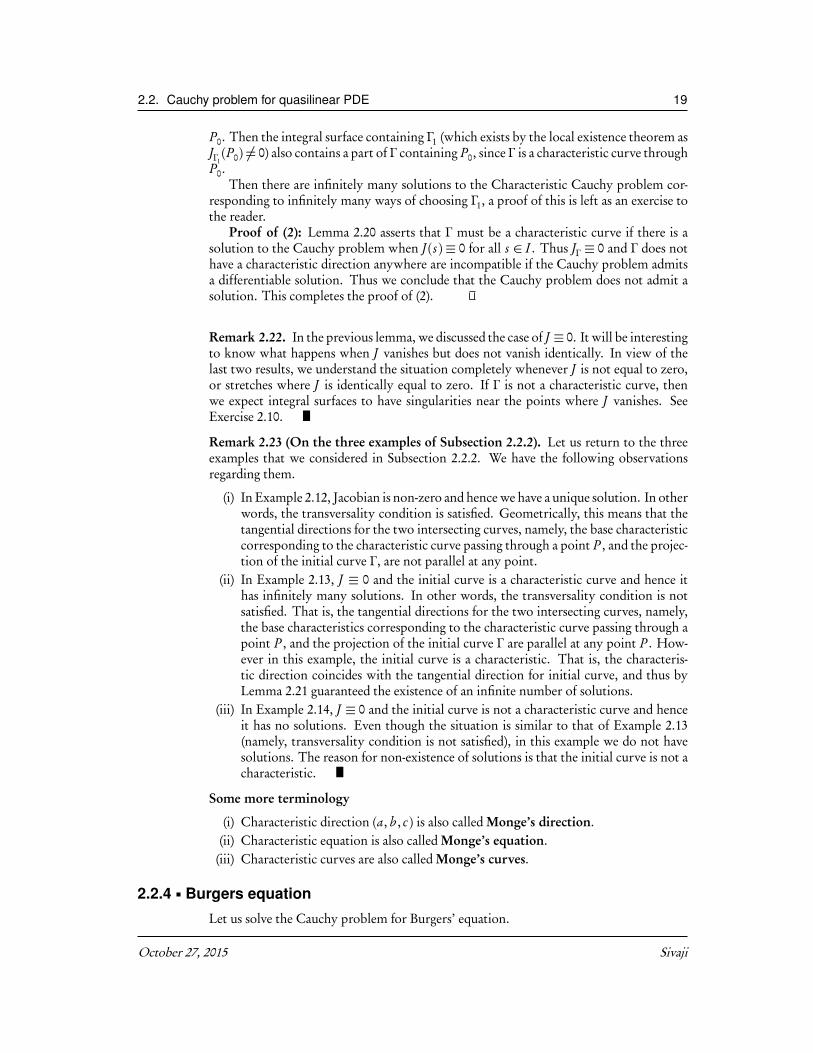
Figure 2.3. Example 2.27: characterisitcs and the solution

Minimum value of y0 is obtained when s2 = 1 and s1 is arbitrary, and equals 1. Thecorresponding value of x0 is then given by x0 = 1. The minimum value of y0 ass1 varies in (0,1), and s2 varies in [1,∞) is the first time that some member of thefamily F2 intersects a member of the family F3, is obtained when s1 = 0 and s2 = 1,and is equal to 1. The corresponding value of x0 is then given by x0 = 1. In otherwords, γ1 intersects γ0 at the point (1,1), as illustrated in Figure 2.3.

(vi) If 1≤ s1 < s2, then γs1and γs2

do not intersect as they are parallel to the line x = 1.

From the above observations on base characteristics, note that for y < 1, a unique basecharacteristic passes through every point (x, y) in the upper half-plane and thus solutionis uniquely determined and is given by

u(x, y) =

1 if x ≤ y,

1−x1−y if y ≤ x ≤ 1,0 if x ≥ 1.

(2.68)

For y > 1, solution is determined in the region to the left of the line x = 1, andin the region bounded by the line y = x and x-axis as exactly one base characteristicpasses through every point of these regions. Solution becomes multivalued in the regionbounded by the lines y = x and x = 1.

At y = 1 the solution breaks down as u becomes multi-valued at the point (1,1). Aweak solution to this problem will be obtained in Section 2.3.

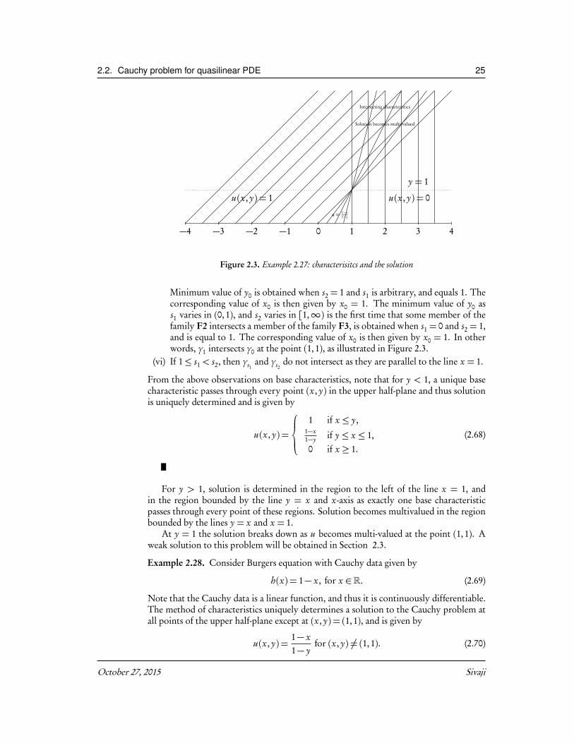
Example 2.28. Consider Burgers equation with Cauchy data given by

h(x) = 1− x, for x ∈R. (2.69)

Note that the Cauchy data is a linear function, and thus it is continuously differentiable.The method of characteristics uniquely determines a solution to the Cauchy problem atall points of the upper half-plane except at (x, y) = (1,1), and is given by

u(x, y) =1− x1− y

for (x, y) = (1,1). (2.70)

October 27, 2015 Sivaji

26 Chapter 2. First order PDE

..

y = 1

.

u(x, y) = 1−x1−y

.−4

.−3

.−2

.−1

.0.

1.

2.

3.

4

Figure 2.4. Example 2.28: characterisitcs and the solution

At (x, y) = (1,1), all the characteristics meet, and hence solution becomes multi-valued asillustrated in Figure 2.4. Note that there are regions in upper half-plane through whichno base characteristic passes in Figure 2.4, but this conclusion is wrong, since the figureis draws only for a limited range of x. Base characteristics emanating from points on thepositive (respectively, negative) x-axis fill-up the second (respectively, first) quadrants.

Intersecting characterisitcs and Gradient catastrophe

In Example 2.27, it was observed that exactly one base characteristic passes through everypoint (x, y) with y < 1, and for every y ≥ 1 there exists a point (x, y) through which twoor more base characterisitcs pass. Thus y = 1 is the critical value as far as crossing of basecharacterisitcs is concerned. The graphs of u(x, y) are shown for y = 0,0.25,0.5,0.75,0.9in Figure 2.5, from which we observed that the graph of x 7→ u(x, y) becomes steeper asy→ 1. This phenomenon is referred to as gradient catastrophe. In this example gradientcatastrophe arises as a result of intersecting base characterisitcs on which u carries distinctvalues. For instance, the base characteristics y = x, x = 1 meet at the point (1,1), and utakes the values 1 and 0 respectively on the base characteristics y = x and x = 1.

Let γs1and γs2

be two base characteristics corresponding to Burgers’ equation (posedon the upper half-plane i.e., y > 0) with Cauchy data u(x, 0) = h(x). We know that γs1

and γs2are straight lines, and are given by the equations

γs1: x = h(s1)y + s1,

γs2: x = h(s2)y + s2.

If γs1and γs2

intersect at a point (x0, y0), then

x0 =h(s1)s2− h(s2)s1

h(s1)− h(s2), y0 =

s2− s1

h(s1)− h(s2). (2.71)

If the function h is increasing i.e., h(s1) < h(s2) whenever s1 < s2, then s2−s1h(s1)−h(s2)

< 0which rules out the possibility of intersecting base characteristics. On the other hand, if

Sivaji IIT Bombay

2.2. Cauchy problem for quasilinear PDE 27

..Graph of u(x, 0)

.−4

.−3

.−2

.−1

.0.

1.

2.

3.

4

..Graph of u(x, 0.25)

.−4

.−3

.−2

.−1

.0.

1.

2.

3.

4

..Graph of u(x, 0.5)

.−4

.−3

.−2

.−1

.0.

1.

2.

3.

4

..Graph of u(x, 0.75)

.−4

.−3

.−2

.−1

.0.

1.

2.

3.

4

..Graph of u(x, 0.9)

.−4

.−3

.−2

.−1

.0.

1.

2.

3.

4

Figure 2.5. Example 2.27: Development of a Gradient catastrophe at y = 1.

the function h is decreasing then s2−s1h(s1)−h(s2)

> 0 and thus base characteristics do intersect.This would result in a gradient catastrophe as discussed at the beginning of this paragraphin the context of Example 2.27. We corroborate this using explicit computation.

Differentiating both sides of u(x, y) = h(x − y u(x, y)) w.r.t. x we obtain

ux (x, y) = h ′(x − y u(x, y))(1− y ux (x, y)).

Re-arranging terms in the last equation yields

ux (x, y) =h ′(x − y u(x, y))

1+ y h ′(x − y u(x, y))(2.72)

When the point (x, y) lies on a base characteristic passing through (s , 0), then the equation(2.72) takes the form

ux (x, y) =h ′(s)

1+ y h ′(s ).

Thus ux (x, y) will become infinite if

y =− 1h ′(s)

. (2.73)

If h is a decreasing function, then h ′ takes negative values, and there exists a y > 0 satisfyingthe equation (2.73). Thus gradient catastrophe occurs at such a y. The minimum such

October 27, 2015 Sivaji

28 Chapter 2. First order PDE

value of y, is called a critical value of y and breaking time of solution (when y is interpretedas time variable), denoted by yc is given by

yc =− 1mins∈R h ′(s)

. (2.74)

Note that in Example 2.28, h ′(s) =−1, and thus gradient catastrophe occurs at yc = 1,and the derivative of the solution is given by

ux (x, y) =− 11− y

,

from which we conclude that gradient catastrophe occurs only at y = 1.

2.2.5 Domain of dependence, Domain of influence

In this subsection we discuss the concepts of domains of dependence and influence in thecontext of two examples. These concepts are characteristic of hyperbolic partial differen-tial equations. We revisit these concepts in the context of wave equations in Section 5.2.

Example 2.29. Consider the following Cauchy problem

ux + uy = 0, (2.75a)

u(x, 0) = sin x, for x ≥ 0. (2.75b)

The solution of the given Cauchy problem is given by

u(x, y) = sin(x − y) for y ≤ x.

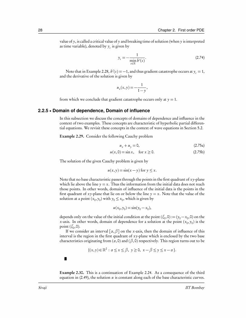
Note that no base characteristic passes through the points in the first quadrant of xy-planewhich lie above the line y = x. Thus the information from the initial data does not reachthose points. In other words, domain of influence of the initial data is the points in thefirst quadrant of xy-plane that lie on or below the line y = x. Note that the value of thesolution at a point (x0, y0) with y0 ≤ x0, which is given by

u(x0, y0) = sin(y0− x0),

depends only on the value of the initial condition at the point (ξ0, 0) := (y0− x0, 0) on thex-axis. In other words, domain of dependence for a solution at the point (x0, y0) is thepoint (ξ0, 0).

If we consider an interval [α,β] on the x-axis, then the domain of influence of thisinterval is the region in the first quadrant of xy-plane which is enclosed by the two basecharacteristics originating from (α, 0) and (β, 0) respectively. This region turns out to be

(x, y) ∈R2 : α≤ x ≤β, y ≥ 0, x −β≤ y ≤ x −α .

Example 2.30. This is a continuation of Example 2.24. As a consequence of the thirdequation in (2.49), the solution u is constant along each of the base characteristic curves.

Sivaji IIT Bombay

32 Chapter 2. First order PDE

2.3 Conservation laws and ShocksThree Cauchy problems for Burgers’ equation were considered in Subsection 2.2.4. Intheir analysis, we came across two kinds of difficulties, namely, either a solution couldnot be determined in some region of the upper half-plane (Example 2.25) or a solutionbecomes multi-valued due to intersecting base characteristics (Examples 2.26 and 2.27).We can overcome these difficulties by suitably modifying the notion of solution, and thesame Cauchy problems will have solutions defined on entire upper half-plane. This is aconsequence of the fact that Burgers equation can be written in the conservative formgiven by

ut +

u2

2

x= 0.

Equations having the conservative form are called conservation laws.In Subsection 2.3.1 we derive a conservation law modeling traffic flow on a highway.

Notion of a weak solution (also called generalized solution) will be introduced in Sub-section 2.3.2, and a result characterizing weak solutions to Conservation laws that arepiecewise smooth will be proved. In Subsection 2.3.3 the notion of a physically relevantentropy solution will be introduced.

In this discussion, we limit ourselves to exhibiting weak solutions and entropy solu-tions for the examples quoted above. Proving the existence of a weak solution (and anentropy soluton) to a general conservation law is beyond the scope of an introductorycourse on PDEs, and hence is omitted.

2.3.1 An example of Conservation law: Traffic flow

Consider traffic flow on a stretch of an express highway with no entry and exit points.Let [a, b ] denote a part of the highway. Let ρ(x, t ) denote the density of cars at x at atime instant t . Then the number of cars in [a, b ] is given by

∫ ba ρ(x, t )d x. The rate of

change of the number of cars is given by q(a)− q(b ). Thus we have

∂

∂ t

∫ baρ(x, t )d x = q(b )− q(a)

Using Leibnitz rule, and the fundamental theorem of calculus, the last equation becomes∫ ba

∂

∂ tρ(x, t )d x =−∫ b

a

∂

∂ xq(x)d x

Thus we get ∫ ba

∂

∂ tρ(x, t )+

∂

∂ xq(x)

d x = 0

Since a, b are arbitrary, we get

∂

∂ tρ(x, t )+

∂

∂ xq(x) = 0

In practice,the flux function q is assumed to be a function of ρ, and thus we write q =F (ρ), and get

∂

∂ tρ(x, t )+

∂

∂ xF (ρ(x, t )) = 0

The last equation is a conservation law.

Sivaji IIT Bombay

2.3. Conservation laws and Shocks 33

2.3.2 Weak solutions

In this paragraph we motivate and introduce a notion of weak solution to a Cauchy prob-lem for a conservation law, so that discontinuous functions may be admitted as solutions.However for consistency reasons, we need to impose certain requirements on the notionof weak solutions. They are

(i) Any smooth solution should also be a weak solution. This motivates the conceptof a weak solution (see Definition 2.32).

(ii) Any weak solution that is smooth should be a classical solution (see Theorem 2.34).(iii) Any “reasonable equation” should have a weak solution, as any notion of a solu-

tion is useless when reasonable equations do not have solutions. We will not bediscussing this issue, as it would take us too far afield.

Let u :R× [0,∞) be a classical soluton to the Cauchy problem

( f (u))y +(g (u))x = 0, (2.86a)

u(x, 0) = h(x), for x ∈R, (2.86b)

where f , g , h :R→R are contiuously differentiable.Multiply the equation (2.86a) with a φ ∈ C∞0 (R× [0,∞)), and integrate w.r.t. x and

y on the domain R× (0,∞) to get∫R

∫ ∞0( f (u))y φ(x, y)d x d y +

∫R

∫ ∞0(g (u))x φ(x, y)d x d y = 0. (2.87)

Integrating by parts in both the integrals of equation (2.87), we get

−∫R

∫ ∞0

f (u)∂ φ

∂ y(x, y)d x d y −∫R

f (h(x))φ(x, 0)d x −∫R

∫ ∞0

g (u)∂ φ

∂ x(x, y)d x d y = 0.

(2.88)

Thus any classical solution u satisfies the equation (2.88). The concept of weak solutionis based on the observation that the equation (2.88) is meaningful for u that are much lessregular than continuously differentiable functions. Depending on the choice of the classof functions for which the equation (2.88) is meaningful, we arrive at different notions ofweak solutions.

In the present discussion, we choose the class L∞loc(R×[0,∞)), for which the equation(2.88) is meaningful. Thus we are led to define the following notion of a weak solution.

Definition 2.32 (weak solution). Let h ∈ L∞loc(R).(i) A function u ∈ L∞loc(R× [0,∞)) is said to be a weak solution of the Cauchy problem

(2.86) if the equation (2.88) is satisfied for all φ ∈C∞0 (R× [0,∞)).(ii) A function u ∈ L∞loc(R× [0,∞)) is said to be a weak solution of the conservation law

(2.86a) if the equation (2.88) is satisfied for all φ ∈C∞0 (R× (0,∞)).

Remark 2.33. The equation (2.88) that defines a weak solution for the Cauchy problem(2.86) is referred to as a weak formulation of the Cauchy problem (2.86).

October 27, 2015 Sivaji

34 Chapter 2. First order PDE

The following result says that if a weak solution is sufficiently smooth, then it is indeeda classical solution.

Theorem 2.34 (Good weak solutions are classical). Let u ∈ C 1(R× (0,∞) ∩C (R×[0,∞)) be a weak solution to the Cauchy problem (2.86). Let f be a one-one function. Thenu is a classical solution of the Cauchy problem (2.86).

Proof. Since u is a weak solution, the identity (2.88) holds for all φ ∈ C∞0 (R× [0,∞)).Since it is given that u is smooth, we can integrte by parts in (2.88) w.r.t. y and x to get

∫R

∫ ∞0( f (u))y φ(x, y)d x d y +

∫R

∫ ∞0(g (u))x φ(x, y)d x d y

+∫R f (u(x, 0)− f (h(x))φ(x, 0)d x = 0. (2.89)

We use this identity with a special choice of test functions φ ∈C∞0 (R×(0,∞)). Usingsuch a φ, the identity (2.89) reduces to∫

R

∫ ∞0

( f (u))y +(g (u))x

φ(x, y)d x d y = 0. (2.90)

Since the identity (2.90) holds for all φ ∈ C∞0 (R× (0,∞)), it follows (by fundamentallemma in calculus of variations) that

∂

∂ yf (u)+

∂

∂ xg (u) = 0 on R× (0,∞). (2.91)

This implies that u satisfies the conservation law (2.86a). Using this information, namely(2.91), the equation (2.89) reduces to

∫R f (u(x, 0)− f (h(x))φ(x, 0)d x = 0, (2.92)

for every φ ∈ C∞0 (R× [0,∞)). Note that any arbitrary function in C∞0 (R) arises asφ(x, 0) for some φ ∈C∞0 (R×[0,∞)). Once again, by the fundamental lemma in calculusof variations, we conclude

f (u(x, 0) = f (h(x)), ∀x ∈R. (2.93)

Further if f is a one-one function, we get u(x, 0) = h(x).

The following result characterizes piecewise smooth functions that can be weak solu-tions to the Cauchy problem (2.86) for a conservation law.

Theorem 2.35. LetΩ⊆R2 be a region, and γ be a curve inR2 that dividesΩ into two partssuch that Ω \ γ is composed of two disjoint regions Ω1 and Ω2. Given u1 ∈ C 1(Ω1)∩C (Ω1)and u2 ∈C 1(Ω2)∩C (Ω2), define

u(x, y) =§

u1(x, y) if (x, y) ∈Ω1,u2(x, y) if (x, y) ∈Ω2. (2.94)

Sivaji IIT Bombay

2.3. Conservation laws and Shocks 35

Let the jump in the values of u across γ be denoted by [u]. That is,

[u](x, y) = u2(x, y)− u1(x, y) for (x, y) ∈ γ . (2.95)

Let [ f (u)] and [g (u)] denote the jumps in f (u) and g (u) across γ respectively. The followingstatements are equivalent.

1. u is a weak solution of the conservation law (2.86a).2. (a) u1 and u2 are classical solutions to the equation (2.86a) in the regions Ω1 and Ω2

respectively.(b) Along curve of discontinuity γ , the following jump condition, which is known as

Rankine-Hugoniot condtion, holds:

[ f (u)]ny +[g (u)]nx = 0, (2.96)

where (nx , ny ) denote unit normal to γ . Further if the curve γ is described by(ξ (y), y), Rankine-Hugoniot condition takes the form

dξd y=[g (u)][ f (u)]

. (2.97)

Proof. Step 1: Proof of 1⇒ 2:

By applying the definition of a weak solution to the conservation law withφ ∈C∞0 (Ωi )(i = 1,2), we get (a). Let us derive Rankine-Hugoniot condition along points of γ . Con-sider φ ∈C∞0 (Ω). Using such a φ, the identity (2.88) reduces to∫

Ω

f (u)

∂ φ

∂ y(x, y)+ g (u)

∂ φ

∂ x(x, y)

d x d y = 0. (2.98)

Since Ω is the disjoint union of Ω1 and Ω2, the last equation (2.98) may be re-written as∫Ω1

f (u)

∂ φ

∂ y(x, y)+ g (u)

∂ φ

∂ x(x, y)

d x d y +∫Ω2

f (u)

∂ φ

∂ y(x, y)+ g (u)

∂ φ

∂ x(x, y)

d x d y = 0.

(2.99)

Denoting the unit outward normal to γ w.r.t. Ω1 by (nx , ny ), the unit outward normal toγ w.r.t. Ω2 is given by (−nx ,−ny ). Performing integration by parts in the identity (2.99)yields

−∫Ω1

f (u1)

y +g (u1)

x

φ(x, y)d x d y −

∫γ

f (u1)ny + g (u1)nx

φ(x, y)dσ

−∫Ω2

f (u2)

y +g (u2)

x

φ(x, y)d x d y +

∫γ

f (u2)ny + g (u2)nx

φ(x, y)dσ = 0.

(2.100)

Since u1 and u2 are classical solutions to conservation law (2.86a) by (a), equation (2.100)reduces to ∫

γ

f (u2)− f (u1)

ny +

g (u2)− g (u1)

nx

φ(x, y)dσ = 0. (2.101)

October 27, 2015 Sivaji

36 Chapter 2. First order PDE

Let [ f (u)] and [g (u)] denote the jumps in f (u) and g (u) across γ respectively. Using thearbitrariness of φ in the equation (2.101), we get Rankine-Hugoniot condition

[ f (u)]ny +[g (u)]nx = 0. (2.102)

Further if the curve γ is described by (ξ (y), y), then direction of the normal is given by1,− dξ

d y

. Thus Rankine-Hugoniot condition (2.102) becomes (2.97).

Step 2: Proof of 2⇒ 1: is left as an exercise to the reader.

Remark 2.36. Note that for each k ∈N, Burgers’ equation uy + u ux = 0 can be writtenin the conservative form

uk

k

y+

uk+1

k + 1

x= 0.

Note that Rankine-Hugoniot condition also depends on k. Let k1 = k2, and u and vbe weak solutions corresponding to k1 and k2 respectively. Then v may not be a weaksolution corresponding to k1, u may not be a weak solution corresponding to k2.

Remark 2.37 (to be read only once). Remember we consider only solutions with onediscontinuity. A good question is why not two? three? infinitely many? We cant handleinfinitely many things. Finitely many case must be similar to the case of two and this canbe done. But we will not do. Meanwhile solve Burgers’ equation with Cauchy data givenby

h(x) =

1 if x ≤ 0,

1− x if 0≤ x ≤ 1,0 if 1≤ x ≤ 2,

1− x2 if x ≥ 2.

Also find a weak solution.

Weak solutions are not unique

The following example illustrates the fact that weak solutions are not unique in general.

Example 2.38 (Example 2.25 revisited). Burgers equation with Cauchy data given by

h(x) =§ −1 if x < 0,

1 if x ≥ 0

has many weak solutions. A few of them are given below.

(i)

u1(x, y) =

−1 if x <−y,

xy if − y < x < y,1 if x > y.

Sivaji IIT Bombay

2.3. Conservation laws and Shocks 37

..

x =y

.

x =−y

.

u(x, y) =−1

.

u(x, y) = 1

.

u(x, y) = xy

Figure 2.6. Example 2.38: Weak solution u1

..

x=

0

.

u(x, y) =−1

.

u(x, y) = 1

Figure 2.7. Example 2.38: Weak solution u2

Note that u1 is a continuous function on the upper half-plane, and is also piecewisesmooth. The function u1 is a classical solution of Burgers’ equation in the regionswhere it is smooth. Since u1 is a continuous function, the Rankine-Hugoniot con-dition is automatically satisfied. Thus u1 is a weak solution to the given Cauchyproblem. See Figure 2.6 for an illustration.

(ii)

u2(x, y) =§ −1 if x < 0,

1 if x > 0.

Note that u2 is a piecewise smooth function with jump across the y-axis. The func-tion u2 is a classical solution of Burgers’ equation in the first and second quadrantswhere it is smooth. Rankine-Hugoniot condition is also satisfied along the y-axis.Thus u2 is a weak solution to the given Cauchy problem. See Figure 2.7 for anillustration.

October 27, 2015 Sivaji

38 Chapter 2. First order PDE

..

x=

0

.

x =1+

a2y

.

x =− 1+a2 y

.

u(x, y) =−1

.

u(x, y) = 1

.

u(x, y) =−a

.

u(x, y) = a

Figure 2.8. Example 2.38: Weak solution u3

(iii) Let a >−1 be any real number. Consider the function u3 defined by

u3(x, y) =

−1 if x < −1−a

2 y,

−a if −1−a2 y < x < 0,

a if 0< x < 1+a2 y,

1 if x > 1+a2 y.

Note that u3 is a piecewise constant function with jumps across three lines: x =−1−a

2 y, x = 0, and x = 1+a2 y. Rankine-Hugoniot condition is satisfied along each

of these lines, and thus u3 is a weak solution to the given Cauchy problem. SeeFigure 2.8 for an illustration.

Thus weak solutions to a Cauchy problem need not be unique.

Example 2.39 (Example 2.26 revisited). Burgers equation with Cauchy data given by

h(x) =§

1 if x < 0,−1 if x ≥ 0

has many weak solutions. A few of them are given below.

(i)

u1(x, y) =§

1 if x < 0,−1 if x > 0.

Note that u1 is a piecewise smooth function with jump across the y-axis. The func-tion u1 is a classical solution of Burgers’ equation in the first and second quadrantswhere it is smooth. Rankine-Hugoniot condition is also satisfied along the y-axis.Thus u1 is a weak solution to the given Cauchy problem. See Figure 2.9 for anillustration.

Sivaji IIT Bombay

2.3. Conservation laws and Shocks 39

..

x=

0

.

u(x, y) = 1

.

u(x, y) =−1

Figure 2.9. Example 2.39: Weak solution u1

..

x=

0

.

x =−1+

a

2

y

.

x = 1−a2 y

.

u(x, y) = 1

.

u(x, y) =−1

.

u(x, y) =−a

.

u(x, y) = a

Figure 2.10. Example 2.39: Weak solution u2

(ii) Let a > 1 be any real number. Consider the function u3 defined by

u2(x, y) =

1 if x < 1−a

2 y,

−a if 1−a2 y < x < 0,

a if 0< x < −1+a2 y,

−1 if x > −1+a2 y.

Note that u2 is a piecewise constant function with jumps across three lines: x =1−a

2 y, x = 0, and x = −1+a2 y. Rankine-Hugoniot condition is satisfied along each

of these lines, and thus u2 is a weak solution to the given Cauchy problem. SeeFigure 2.10 for an illustration.

October 27, 2015 Sivaji

40 Chapter 2. First order PDE

..x =

y

.

x=

1

.

x=

y+1

2

.

(1,1)

.

u(x, y) = 0

.

u(x, y) = 1

.u = 1−x

1−y

Figure 2.11. Example 2.40: Weak solution u

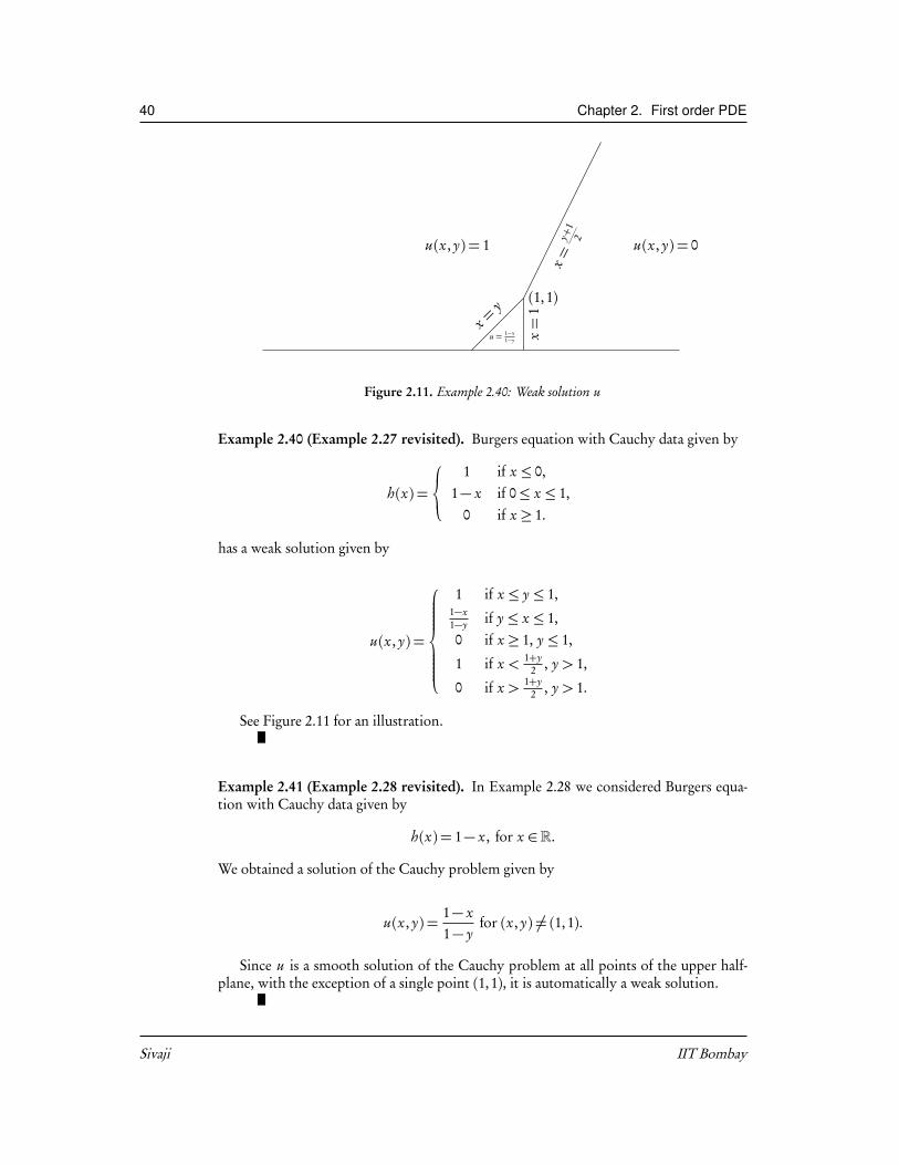
Example 2.40 (Example 2.27 revisited). Burgers equation with Cauchy data given by

h(x) =

1 if x ≤ 0,

1− x if 0≤ x ≤ 1,0 if x ≥ 1.

has a weak solution given by

u(x, y) =

1 if x ≤ y ≤ 1,1−x1−y if y ≤ x ≤ 1,0 if x ≥ 1, y ≤ 1,

1 if x < 1+y2 , y > 1,

0 if x > 1+y2 , y > 1.

See Figure 2.11 for an illustration.

Example 2.41 (Example 2.28 revisited). In Example 2.28 we considered Burgers equa-tion with Cauchy data given by

h(x) = 1− x, for x ∈R.

We obtained a solution of the Cauchy problem given by

u(x, y) =1− x1− y

for (x, y) = (1,1).

Since u is a smooth solution of the Cauchy problem at all points of the upper half-plane, with the exception of a single point (1,1), it is automatically a weak solution.

Sivaji IIT Bombay

2.3. Conservation laws and Shocks 41

2.3.3 Entropy solutions

Since classical solutions are not defined for all t > 0, even for smooth initial data, werelaxed the notion of solution to a weak solution. However we observed in the last sub-section that a Cauchy problem may admit more than one weak solution. Thus we seekconditions that identify a ‘physically relevant’ weak solution, among all possible weaksolutions to a Cauchy problem. This leads us to the notion of entropy solution.

In this subsection we define the notion of weak solution, and then identify entropysolutions for the examples considered in the last subsection. It turns out that entropysolution is unique, and further discussion on entropy solutions may be found in [39].

Consider the Cauchy problem for a conservation law with strictly convex flux givenby

uy +(g (u))x = 0, (2.103a)

u(x, 0) = h(x), for x ∈R, (2.103b)

where g ∈C 2(R) is a strictly convex function, and g ∈C 1(R).We know that the solution to (2.103) is implicitly given by u(x, y) = h(x − y g ′(u)).

On differentiating w.r.t. x, and simiplifying we get

ux (x, y) =h ′(x − y u(x, y))

1+ g ′′(u)y h ′(x − y u(x, y)). (2.104)

Note that if h ′ > 0, then from (2.104) we get

ux (x, y)<1

C y, (2.105)

where C > 0 is such that g ′′(u)> C for all u ∈R. Using mean value theorem we get forh > 0,

u(x + h, y)− u(x, y) = ux (ξ , y)h <1

C yh. (2.106)

This motivates the following definition of an entropy solution.

Definition 2.42. A piecewise continuous function u is said to be an entropy solution to theCauchy problem (2.103) if u is a weak solution to (2.103) satisfying the entropy condition, i.e.,there exists a C > 0 such that for every (x, y, h) ∈R× (0,∞)× (0,∞), the following entropyinequality holds

u(x + h, y)− u(x, y)<Cy

h. (2.107)

The following result summarizes some of the important properties of entropy solu-tions.

Lemma 2.43. Let u be an entropy solution to the Cauchy problem (2.103). Then

1. the function u can have at most a countable number of jump discontinuities.

October 27, 2015 Sivaji

42 Chapter 2. First order PDE

2. For a fixed y > 0, let the function x 7→ u(x, y) be discontinuous at the point x0. Thenu+ < u−, where

u− = limx→x0−

u(x, y), u+ = limx→x0+

u(x, y).

3. For a strictly convex flux g ∈C 2(R),

g ′(u+)<g (u+)− g (u−)

u+− u−< g ′(u−). (2.108)

Proof. Proof of (i): From the entropy condition it follows that for each fixed y > 0, thefunction

u(x, y)− Cy

x

is a decreasing function. Since a monotonic function can have at most a countable numberof jump discontinuities, statement (i) follows.

Proof of (ii): Consider points x1, x2 satisfying x1 < x0 < x2. Since the function

u(x, y)− Cy

x

is a decreasing function, we get

u(x2, y)− Cy

x2 < u(x1, y)− Cy

x1

Taking limit as x1→ x0, and x2→ x0 in the last inequality, we get u+ < u−.Proof of (iii): By mean value theorem, we have

g (u+)− g (u−)u+− u−

= g ′(u∗),

where u∗ ∈ (u+, u−). Since g is strictly convex, its derivative g ′ is an increasing function.As a consequence, we get (2.108).

Remark 2.44.

Since entropy solution to the Cauchy problem (2.103) is unique [39], a weak solutionsatisfying the entropy condition (2.107) is the entropy solution. On the other hand,Lemma 2.43 helps in identifying weak solutions that are not entropy solutions.

In Example 2.38, three weak solutions to a Cauchy problem for Burgers equation (seeExample 2.25) were obtained. The weak solution u1 satisfies the entropy condition, andthus is the entropy solution.

On the other hand, u2 does not satisfy the condition u+ < u− (see (ii) of Lemma 2.43)at x = 0 which is the only point of discontinuity of u2.

The weak solution u3 is also not an entropy solution as the condition (ii) of Lemma 2.43is violated. For, if the condition u+ < u− holds at all discontinuity points of u3, we get1< a and a <−a which are not consistent with each other.

Sivaji IIT Bombay