18. Barotropic instability

Consider an inviscid barotropic flow governed by the barotropic vorticity equation

dη = 0, (18.1)

dt

where

η = ∇2ψ (18.2)

and ψ is the streamfunction. There exists a class of exact solutions of (18.1) char­

acterized by ψ = ψ(y),

d2ψ η = .

dy2

These are just zonal flows that vary meridionally. We have seen that flows with

cross-stream variations of η can support Rossby waves. Now consider a class of

jet-like flows that look like the example shown in Figure 18.1, where there is an

extremum in the vorticity. In the example given, there is a maximum of vorticity in

the center of the domain, with westward flow to the north and eastward flow to the

south. The meridional gradient of vorticity is negative to the north of the vorticity

maximum, and positive to the south, so that barotropic Rossby waves propagate

eastward, relative to the flow, to the north; and westward, relative to the flow, to

the south.

Now consider perturbing the flow in Figure 18.1 in the manner shown in Figure

18.2:

83

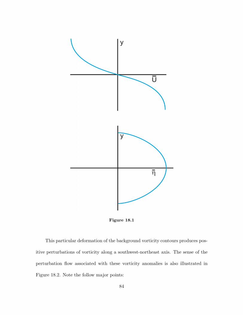
Figure 18.1

This particular deformation of the background vorticity contours produces pos­

itive perturbations of vorticity along a southwest-northeast axis. The sense of the

perturbation flow associated with these vorticity anomalies is also illustrated in

Figure 18.2. Note the follow major points:

84

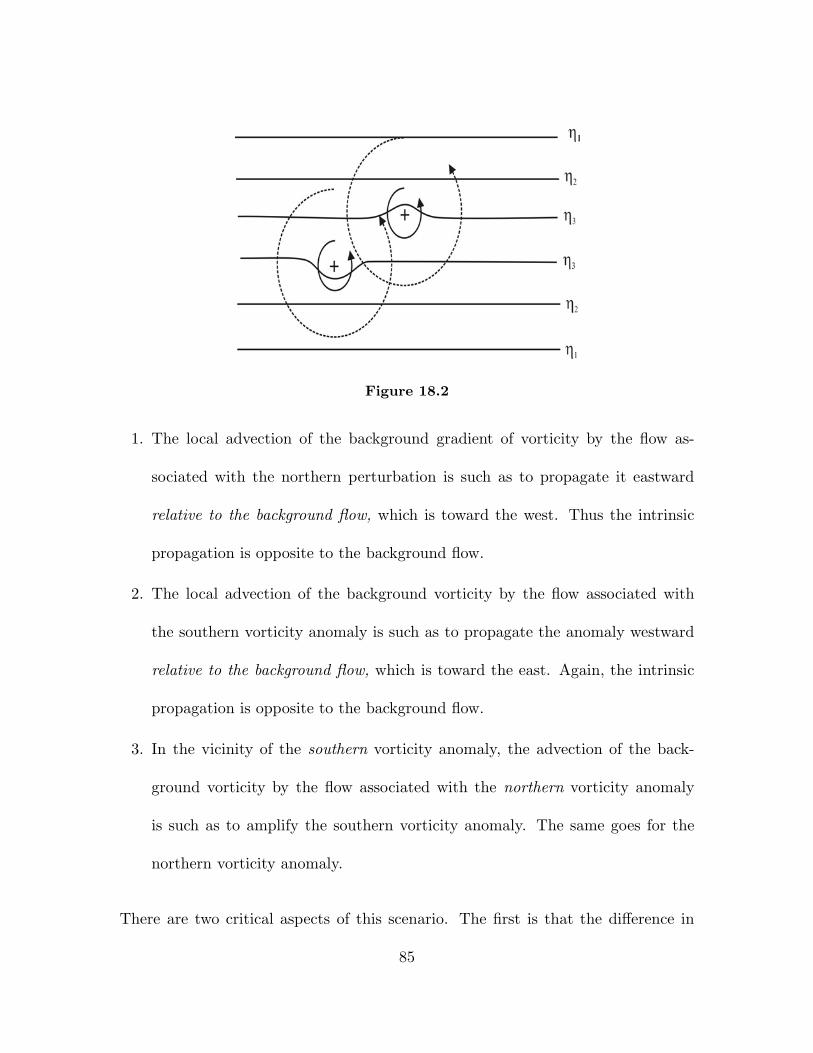
Figure 18.2

1. The local advection of the background gradient of vorticity by the flow as­

sociated with the northern perturbation is such as to propagate it eastward

relative to the background flow, which is toward the west. Thus the intrinsic

propagation is opposite to the background flow.

2. The local advection of the background vorticity by the flow associated with

the southern vorticity anomaly is such as to propagate the anomaly westward

relative to the background flow, which is toward the east. Again, the intrinsic

propagation is opposite to the background flow.

3. In the vicinity of the southern vorticity anomaly, the advection of the back­

ground vorticity by the flow associated with the northern vorticity anomaly

is such as to amplify the southern vorticity anomaly. The same goes for the

northern vorticity anomaly.

There are two critical aspects of this scenario. The first is that the difference in

85

the intrinsic phase speeds of the two anomalies is compensated by the different ad­

vections of the anomalies by the background flow, creating the possibility that the

anomalies can be phase locked with one another. The second is that the anomalies

can be mutually amplifying; i.e., each anomaly amplifies the other anomaly. These

two aspects are critical to the process called barotropic instability. In the follow­

ing section, we find analytic solutions to a particular example of a barotropically

unstable flow.

86

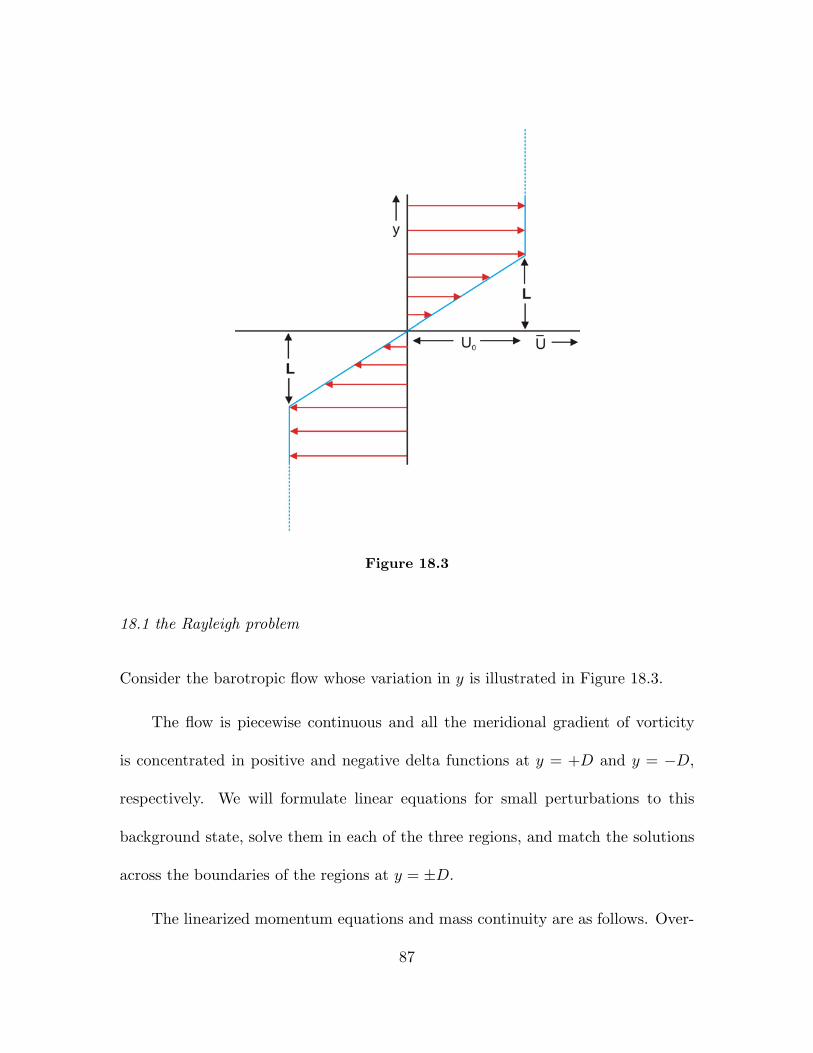
Figure 18.3

18.1 the Rayleigh problem

Consider the barotropic flow whose variation in y is illustrated in Figure 18.3.

The flow is piecewise continuous and all the meridional gradient of vorticity

is concentrated in positive and negative delta functions at y = +D and y = −D,

respectively. We will formulate linear equations for small perturbations to this

background state, solve them in each of the three regions, and match the solutions

across the boundaries of the regions at y = ±D.

The linearized momentum equations and mass continuity are as follows. Over­

87

( )

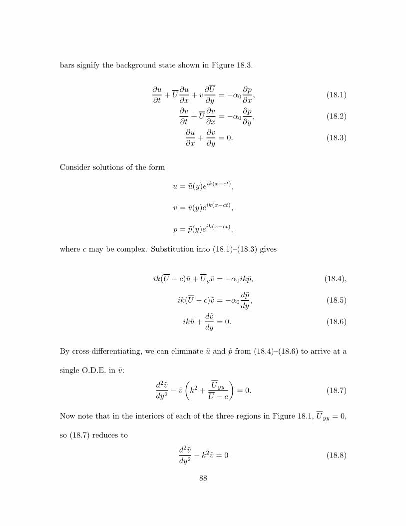
bars signify the background state shown in Figure 18.3.

∂u ∂t

+ U ∂u ∂x

+ v ∂U ∂y

= −α0 ∂p ∂x, (18.1)

∂v ∂t

+ U ∂v ∂x

= −α0 ∂p ∂y, (18.2)

∂u ∂x

+ ∂v ∂y

= 0. (18.3)

Consider solutions of the form

u = u(y)e ik(x−ct),

v = v(y)e ik(x−ct),

p = p(y)e ik(x−ct),

where c may be complex. Substitution into (18.1)–(18.3) gives

ik(U − c)u + Uy v = −α0ikp, (18.4),

dpik(U − c)v = −α0 , (18.5)

dy

dviku+ = 0. (18.6)

dy

By cross-differentiating, we can eliminate u and p from (18.4)–(18.6) to arrive at a

single O.D.E. in v:

d2v − v k2 + Uyy = 0. (18.7)

dy2 U − c

Now note that in the interiors of each of the three regions in Figure 18.1, Uyy = 0,

so (18.7) reduces to

d2v − k2 v = 0 (18.8)dy2

88

( )

within each region. Now we consider boundary conditions for solving (18.8). First

we impose the condition that the solutions remain bounded at y = ±∞:

lim v = finite. y→±∞

General solutions of (18.8) that satisfy this condition are:

I: v = Ae−ky

II: v = Be−ky + Ceky (18.9)

III: v = Feky

Next we apply boundary conditions at the boundaries separating the regions. There

are two fundamental requirements:

a. Fluid displacements must be continuous, and

b. Pressure must be continuous.

The displacement in y, δy, is related to v by

d v ≡ δy.

dt

Linearizing this about the background state gives

∂ ∂ v = + U δy,

∂t ∂x

and substituting

δy = δyeik(x−ct),

we have

v = ik(U − c)δy.

89

[ ]

Continuity of δy demands that

vis continuous. (18.10)

ik(U − c)

In the present case, U itself is continuous, so (18.10) implies that v is continuous.

Continuity of pressure implies, through (18.4), that the quantity

ik(U − c)u + Uy v

is continuous, or using (18.6) to eliminate iku,

dv(U − c) − Uy v is continuous. (18.11)

dy

Matching v and the quantity given by (18.11) across each of the two boundaries in

the general solutions (18.9) gives a condition on the relation between the complex

phase speed c and k: ( )2Dkc

= (Dk − 1)2 − e −2kD . (18.12)U0

Here we see that c is purely real if (Dk − 1)2 ≥ e−2kD, and purely imaginary if

(Dk − 1)2 < e−2kD . In the former case, examination of (18.12) shows that to order

1/k,

2lim c = ±U0 1 − . (18.13)

k→∞ kD

Very small-scale perturbations are confined to the delta function vorticity gradients

at y = ± 12 D and move with the mean flow speed at the respective boundaries

between regions, slightly slowed down owing the Rossby propagation effect.

90

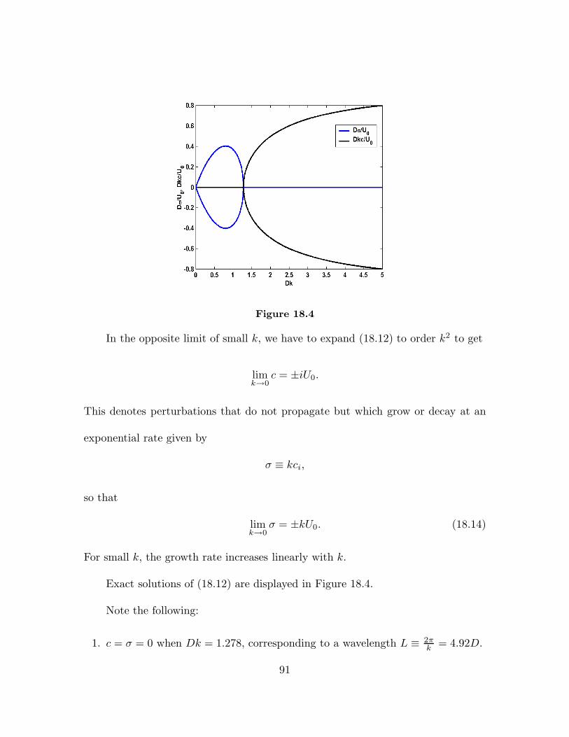
Figure 18.4

In the opposite limit of small k, we have to expand (18.12) to order k2 to get

lim c = ±iU0. k→0

This denotes perturbations that do not propagate but which grow or decay at an

exponential rate given by

σ ≡ kci,

so that

lim σ = ±kU0. (18.14) k→0

For small k, the growth rate increases linearly with k.

Exact solutions of (18.12) are displayed in Figure 18.4.

Note the following:

1. c = σ = 0 when Dk = 1.278, corresponding to a wavelength L ≡ 2kπ = 4.92D.

91

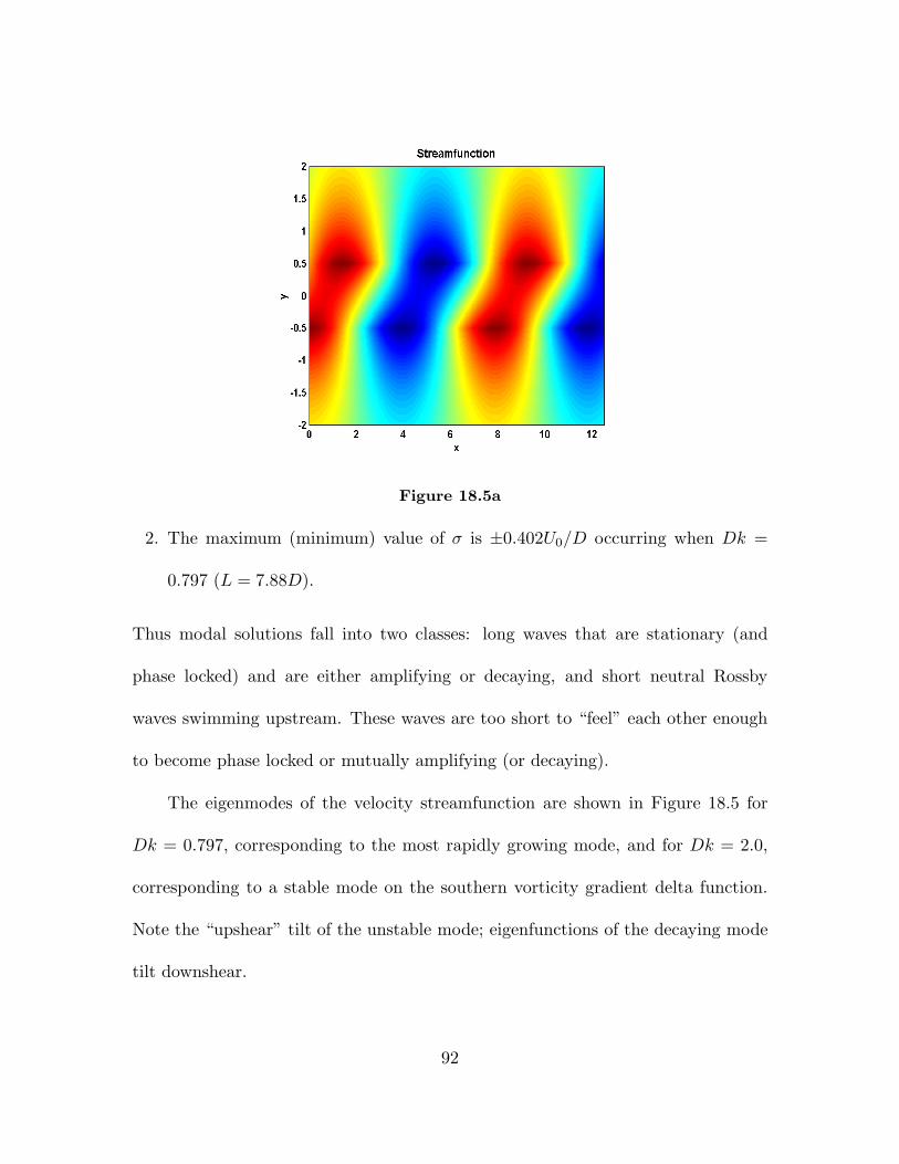
Figure 18.5a

2. The maximum (minimum) value of σ is ±0.402U0/D occurring when Dk =

0.797 (L = 7.88D).

Thus modal solutions fall into two classes: long waves that are stationary (and

phase locked) and are either amplifying or decaying, and short neutral Rossby

waves swimming upstream. These waves are too short to “feel” each other enough

to become phase locked or mutually amplifying (or decaying).

The eigenmodes of the velocity streamfunction are shown in Figure 18.5 for

Dk = 0.797, corresponding to the most rapidly growing mode, and for Dk = 2.0,

corresponding to a stable mode on the southern vorticity gradient delta function.

Note the “upshear” tilt of the unstable mode; eigenfunctions of the decaying mode

tilt downshear.

92

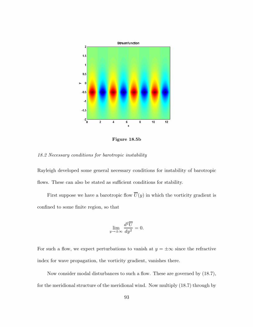
Figure 18.5b

18.2 Necessary conditions for barotropic instability

Rayleigh developed some general necessary conditions for instability of barotropic

flows. These can also be stated as sufficient conditions for stability.

First suppose we have a barotropic flow U(y) in which the vorticity gradient is

confined to some finite region, so that

d2U = 0.lim

y→±∞ dy2

For such a flow, we expect perturbations to vanish at y = ±∞ since the refractive

index for wave propagation, the vorticity gradient, vanishes there.

Now consider modal disturbances to such a flow. These are governed by (18.7),

for the meridional structure of the meridional wind. Now multiply (18.7) through by

93

[ ( )]

∣ ∣ ∣

∣ ∣ ∣

[ ]

∣ ∣

the complex conjugate of v, v ∗, and integrate the result through the whole domain:

∫ ∞

v∗

dy

d2v2 − |v|2 k2 +

Uyy dy = 0 (18.15)

−∞ U − c

Here we have made use of the fact that

vv∗ = |v|2 ,

where |v| is the absolute value of v. Now the first term in the integrand can be

integrated by parts:

∫ ∞∗ d

2v∫ ∞ d

[ ∗ dv

] ∫ ∞ ∣∣ dv ∣∣ 2

v dy = v dy − ∣ dy. −∞ dy2 −∞ dy dy −∞ dy

The first term on the right can be integrated exactly, but it vanishes because v → 0

as y → ±∞. Thus ∫ ∞ ∫ ∞ ∣ ∣2d2v ∣ dv ∣ v dy = − ∣ dy. (18.16)

−∞ dy2 −∞ dy

Using (18.16), we may write (18.15) as

∫ ∞ ∣ ∣2 ∣ dv ∣ ( )∣ ∣ + |v|2 k2 + Uyy

dy = 0. (18.17)−∞ dy U − c

Remember that c is, in general, complex, so the real and imaginary parts of (18.17)

must both be satisfied. The imaginary part of (18.17) is

∫ ∞

ci Uyy |v|2dy = 0, (18.18)

−∞ |U − c|2

where ci is the imaginary part of c, which is positive for growing disturbances.

The relation (18.18) shows that one of two things must be true: Either

94

[ ] ∣ ∣ ∣ ∣

∫ [ ] ∣ ∣ ∣ ∣ ∣ ∣

a. ci = 0, or

b. the integral in (18.18) vanishes.

Thus we may conclude the following:

1. A necessary condition for instability (ci > 0) is that Uyy change sign at least

once within the domain. In other words, the mean state vorticity must have

an extremum in the domain. But note that even if Uyy does change sign, this

is no guarantee that the integral vanishes or that ci > 0. This condition is not

sufficient for instability.

2. If there is no extremum of vorticity within the domain, ci = 0 and this is

therefore a sufficient condition for stability.

Points 1 and 2 are really saying the same thing.

Another theorem, due to Fjøtoft, may be derived by looking at the real part

of (18.17):

∫ ∫ ∣ ∣2∞ ∞Uyy(U − cr) |v|2dy = − ∣ dv ∣ + k2|v|2 dy, (18.19) −∞ |U − c|2 −∞ dy

where cr is the real part of c. Note that for growing disturbances, we are free to add

any multiple of the integral in (18.18) to the left side of (18.19), since the former

vanishes. We choose the multiplying factor to be cr, giving

∫ ∞ ∞ ∣ dv ∣ 2UUyy |v|2dy = − + k2|v|2 dy. (18.20) −∞ |U − c|2 −∞ dy

Since the right-hand side of (18.20) is negative definite, so must the left side. So

fluctuations of U must be negatively correlated with Uyy for growing disturbances.

95

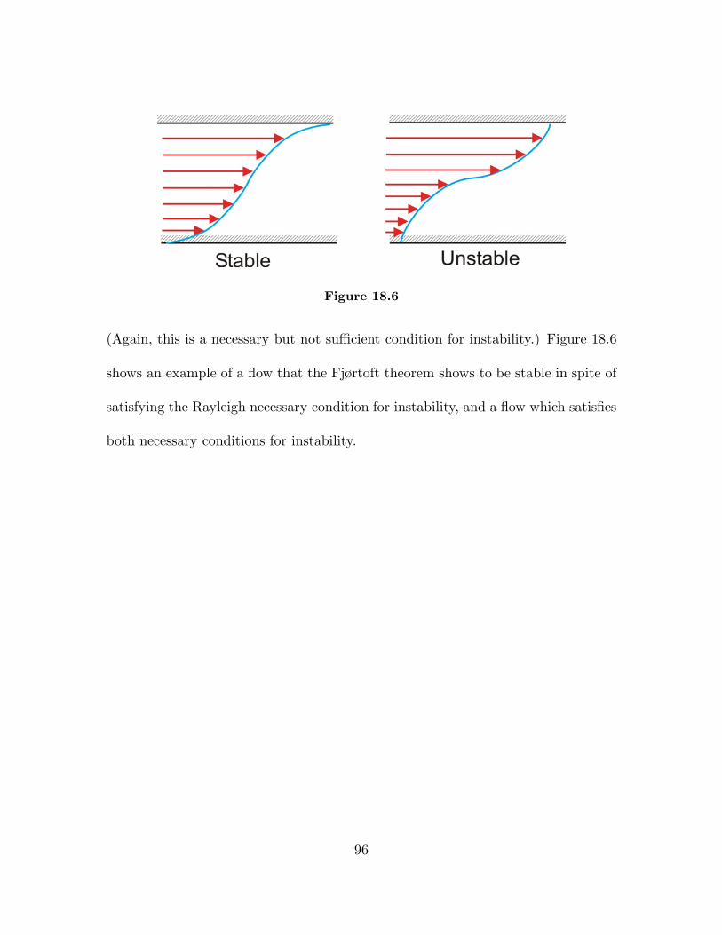
Figure 18.6

(Again, this is a necessary but not sufficient condition for instability.) Figure 18.6

shows an example of a flow that the Fjørtoft theorem shows to be stable in spite of

satisfying the Rayleigh necessary condition for instability, and a flow which satisfies

both necessary conditions for instability.

96

MIT OpenCourseWarehttp://ocw.mit.edu

12.803 Quasi-Balanced Circulations in Oceans and Atmospheres Fall 2009

For information about citing these materials or our Terms of Use, visit: http://ocw.mit.edu/terms.