


γλώσσες
Σελίδες
Νομικός

Nonlinear Inverse Problems Simulated Annealing
),(),(),(),(
mdmdmdkmd
µθρσ = Simulated AnnealingSimulated Annealing
• What is simulated annealing?
• Simulated annealing and probabilistic inversion
• Examples
• What is simulated annealing?
• Simulated annealing and probabilistic inversion
• Examples
The problem: we need to efficiently search a possibly multi-modal function in order to either sample the function or find the maximum-likely point of of that function.
We draw on an analogy from solid state physics: the annealing process.

Nonlinear Inverse Problems Simulated Annealing
),(),(),(),(
mdmdmdkmd
µθρσ = Simulated AnnealingSimulated Annealing
Annealing is the process of heating a solid until thermal stresses are released. Then, in cooling it very slowly to the ambient temperature until perfect crystals emerge. The quality of the results strongly depends on the cooling temperature. The final state can be interpreted as an energy state (crystaline potential energy) which is lowest if a perfectly crystal emerged.
Annealing is the process of heating a solid until thermal stresses are released. Then, in cooling it very slowly to the ambient temperature until perfect crystals emerge. The quality of the results strongly depends on the cooling temperature. The final state can be interpreted as an energy state (crystaline potential energy) which is lowest if a perfectly crystal emerged.
But where’s the connection to inverse problems?
Nonlinear Inverse Problems Simulated Annealing
),(),(),(),(
mdmdmdkmd
µθρσ = Simulated AnnealingSimulated Annealing
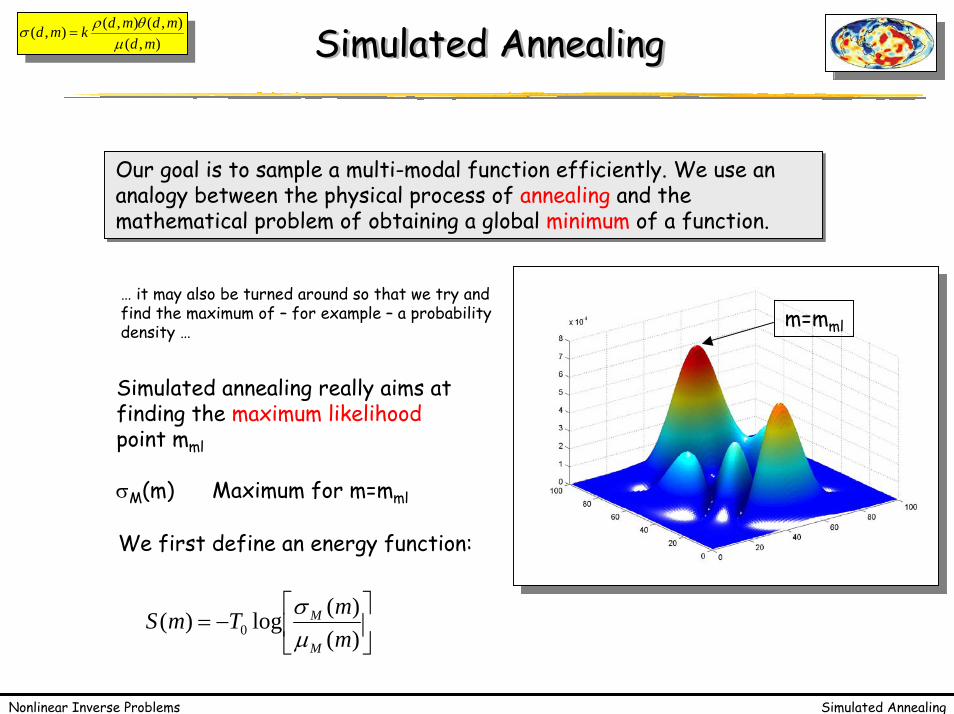
Our goal is to sample a multi-modal function efficiently. We use an analogy between the physical process of annealing and the mathematical problem of obtaining a global minimum of a function.
Our goal is to sample a multi-modal function efficiently. We use an analogy between the physical process of annealing and the mathematical problem of obtaining a global minimum of a function.
… it may also be turned around so that we try and find the maximum of – for example – a probabilitydensity …
m=mml
Simulated annealing really aims at finding the maximum likelihoodpoint mml
σM(m) Maximum for m=mml
We first define an energy function:
⎥⎦
⎤⎢⎣
⎡−=
)()(log)( 0 m
mTmSM
M
µσ
Nonlinear Inverse Problems Simulated Annealing
),(),(),(),(
mdmdmdkmd
µθρσ = Simulated AnnealingSimulated Annealing
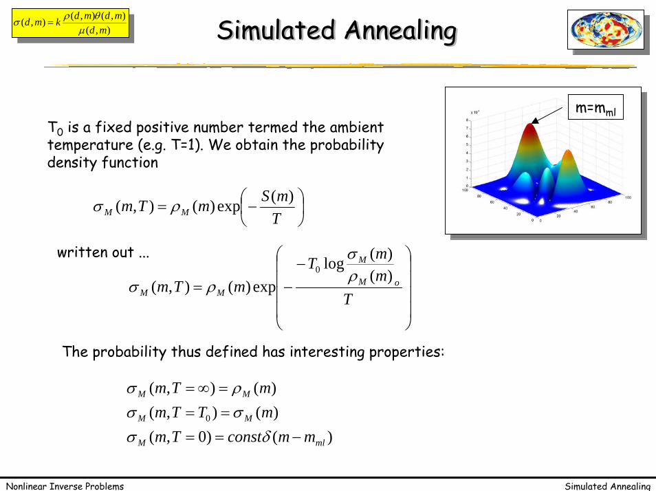
m=mmlT0 is a fixed positive number termed the ambient temperature (e.g. T=1). We obtain the probability density function
⎟⎠⎞
⎜⎝⎛−=
TmSmTm MM
)(exp)(),( ρσ
written out ...
⎟⎟⎟⎟
⎠
⎞
⎜⎜⎜⎜
⎝
⎛ −−=
TmmT
mTm oM
M
MM)()(log
exp)(),(0 ρ
σ
ρσ
The probability thus defined has interesting properties:
)()0,()(),()(),(
0
mlM
MM
MM
mmconstTmmTTmmTm
−=====∞=
δσσσρσ
Nonlinear Inverse Problems Simulated Annealing
),(),(),(),(
mdmdmdkmd
µθρσ = The Heat BathThe Heat Bath
⎟⎟⎟⎟
⎠
⎞
⎜⎜⎜⎜
⎝
⎛ −−=
TmmT
mTm oM
M
MM)()(log
exp)(),(0 ρ
σ
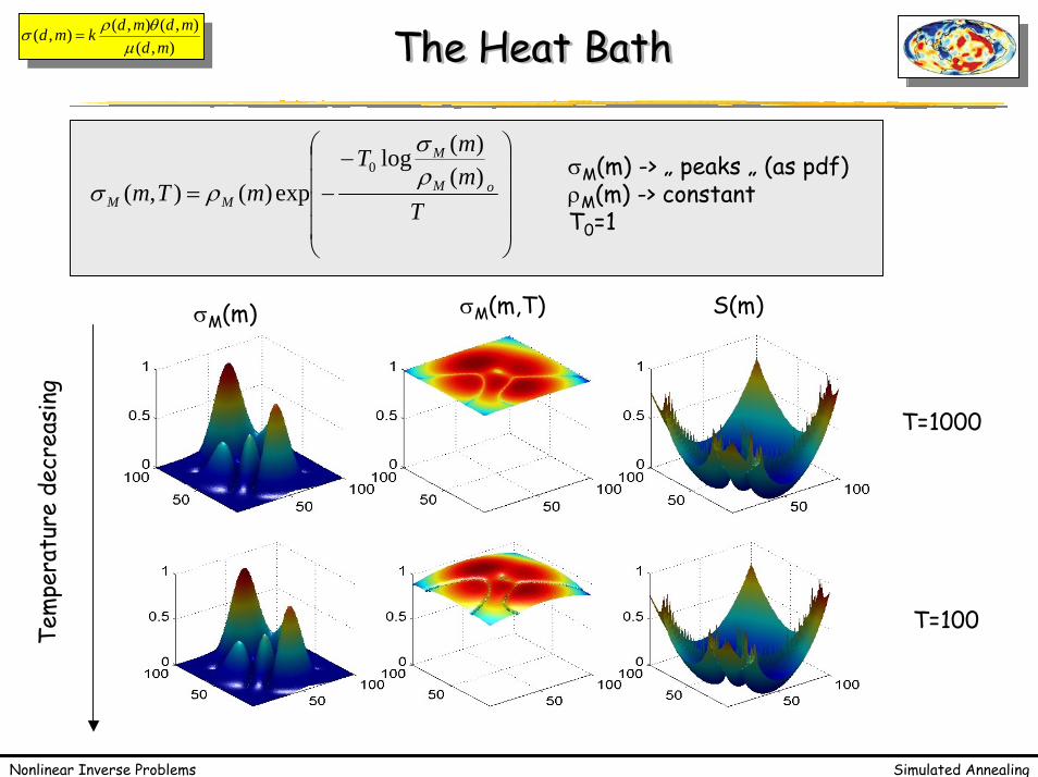
ρσσM(m) -> „ peaks „ (as pdf)ρM(m) -> constantT0=1
σM(m,T)σM(m) S(m)
Tem
pera
ture
dec
reas
ing
T=1000
T=100
Nonlinear Inverse Problems Simulated Annealing
),(),(),(),(
mdmdmdkmd
µθρσ = The Heat BathThe Heat Bath
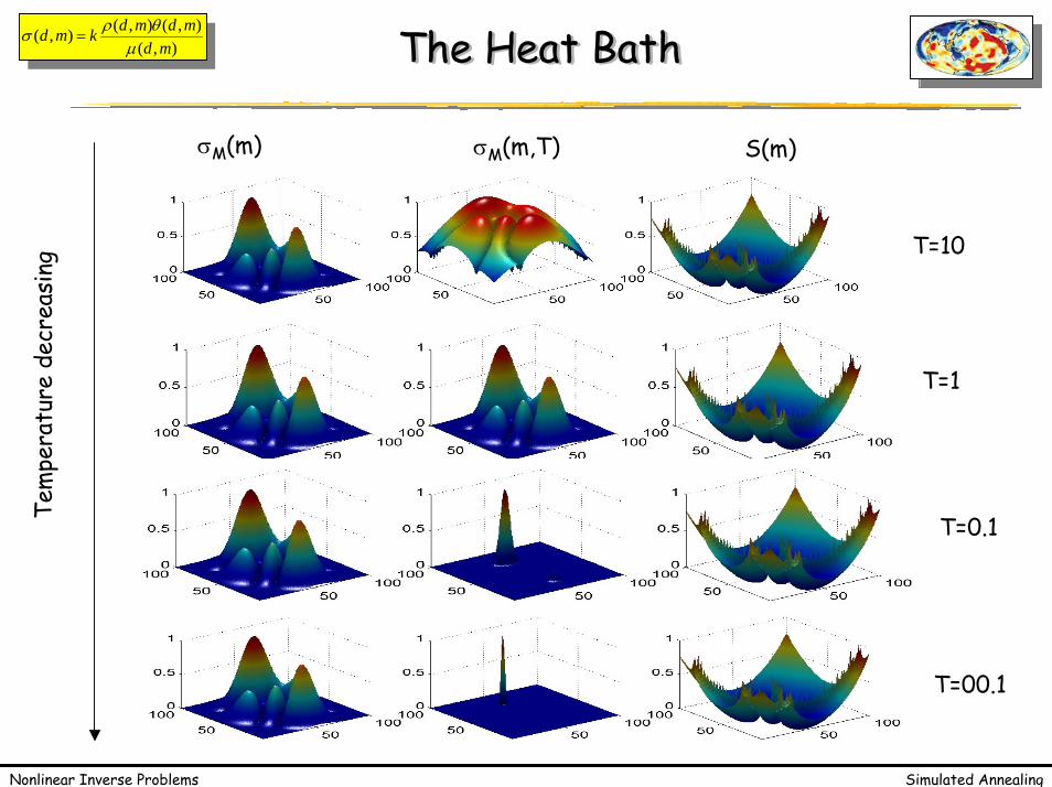
σM(m,T)σM(m) S(m)
T=10
T=1
T=0.1
T=00.1
Tem
pera
ture
dec
reas
ing
Nonlinear Inverse Problems Simulated Annealing
),(),(),(),(
mdmdmdkmd
µθρσ = Simulated AnnealingSimulated Annealing
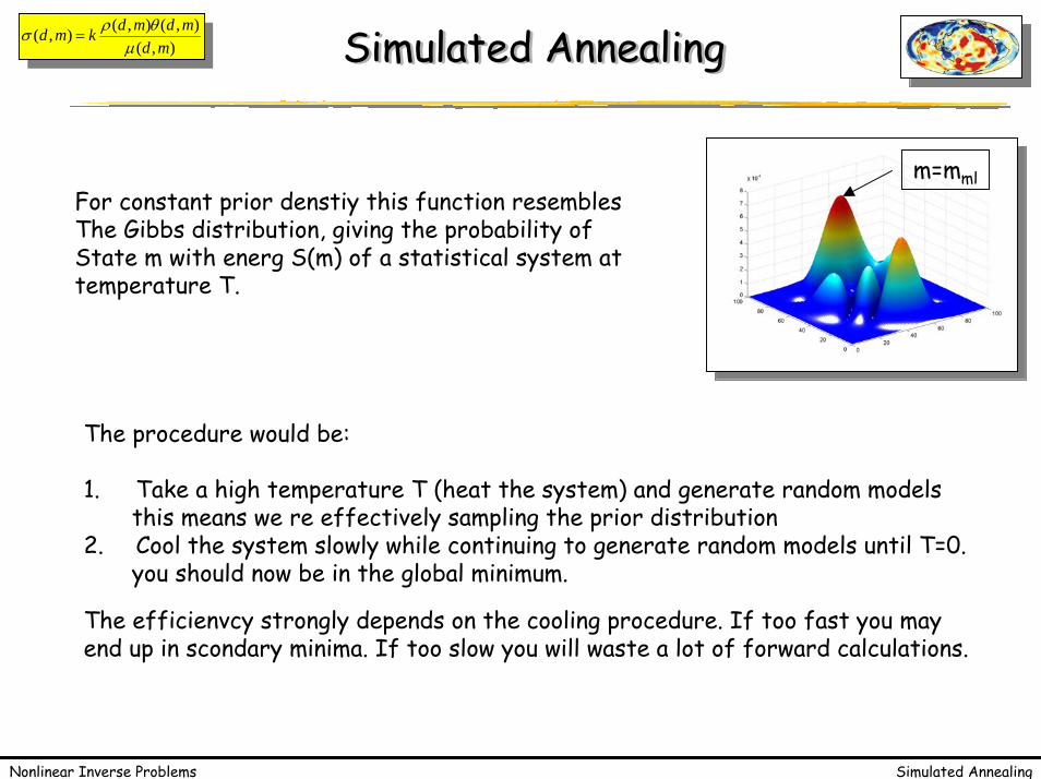
m=mmlFor constant prior denstiy this function resemblesThe Gibbs distribution, giving the probability of State m with energ S(m) of a statistical system at temperature T.
The procedure would be:
1. Take a high temperature T (heat the system) and generate random models this means we re effectively sampling the prior distribution
2. Cool the system slowly while continuing to generate random models until T=0. you should now be in the global minimum.
The efficienvcy strongly depends on the cooling procedure. If too fast you mayend up in scondary minima. If too slow you will waste a lot of forward calculations.
Nonlinear Inverse Problems Simulated Annealing
),(),(),(),(
mdmdmdkmd
µθρσ = Simulated AnnealingSimulated Annealing
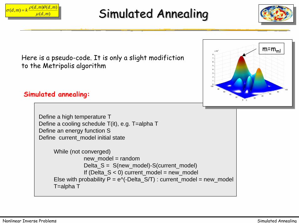
Here is a pseudo-code. It is only a slight modifictionto the Metripolis algorithm
m=mml
Simulated annealing:
Define a high temperature TDefine a cooling schedule T(it), e.g. T=alpha TDefine an energy function SDefine current_model initial state
While (not converged)new_model = randomDelta_S = S(new_model)-S(current_model)If (Delta_S < 0) current_model = new_model
Else with probability P = e^(-Delta_S/T) : current_model = new_modelT=alpha T
Nonlinear Inverse Problems Simulated Annealing
),(),(),(),(
mdmdmdkmd
µθρσ = Simulated AnnealingSimulated Annealing
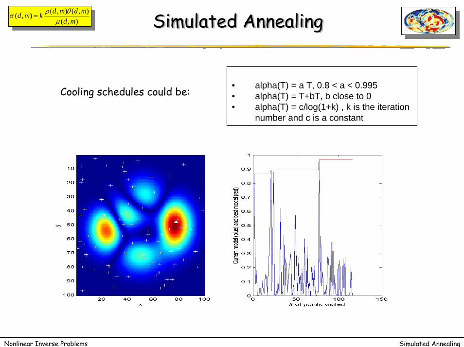
• alpha(T) = a T, 0.8 < a < 0.995• alpha(T) = T+bT, b close to 0• alpha(T) = c/log(1+k) , k is the iteration
number and c is a constant
Cooling schedules could be:
Nonlinear Inverse Problems Simulated Annealing
),(),(),(),(
mdmdmdkmd
µθρσ = Simulated AnnealingSimulated Annealing
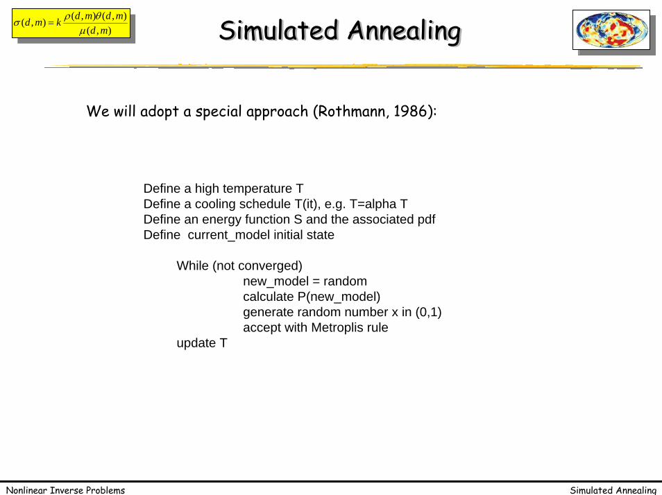
We will adopt a special approach (Rothmann, 1986):
Define a high temperature TDefine a cooling schedule T(it), e.g. T=alpha TDefine an energy function S and the associated pdfDefine current_model initial state
While (not converged)new_model = randomcalculate P(new_model)generate random number x in (0,1)accept with Metroplis rule
update T
Nonlinear Inverse Problems Simulated Annealing
),(),(),(),(
mdmdmdkmd
µθρσ = Simulated AnnealingSimulated Annealing
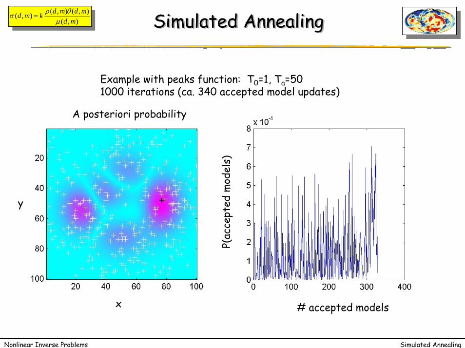
Example with peaks function: T0=1, Ta=501000 iterations (ca. 340 accepted model updates)
P(ac
cept
ed m
odel
s)
# accepted modelsx
y
A posteriori probability
Nonlinear Inverse Problems Simulated Annealing
),(),(),(),(
mdmdmdkmd
µθρσ = SummarySummary
Simulated annealing is an mathematical analogy to a cooling system which can be used to sample highly nonlinear,multidimensional functions.
There are many flavors around and the efficiency strongly depends on the particular function to sample. Therefore it is extremely difficult to make general statements as to whatparameters work best.
Top Related