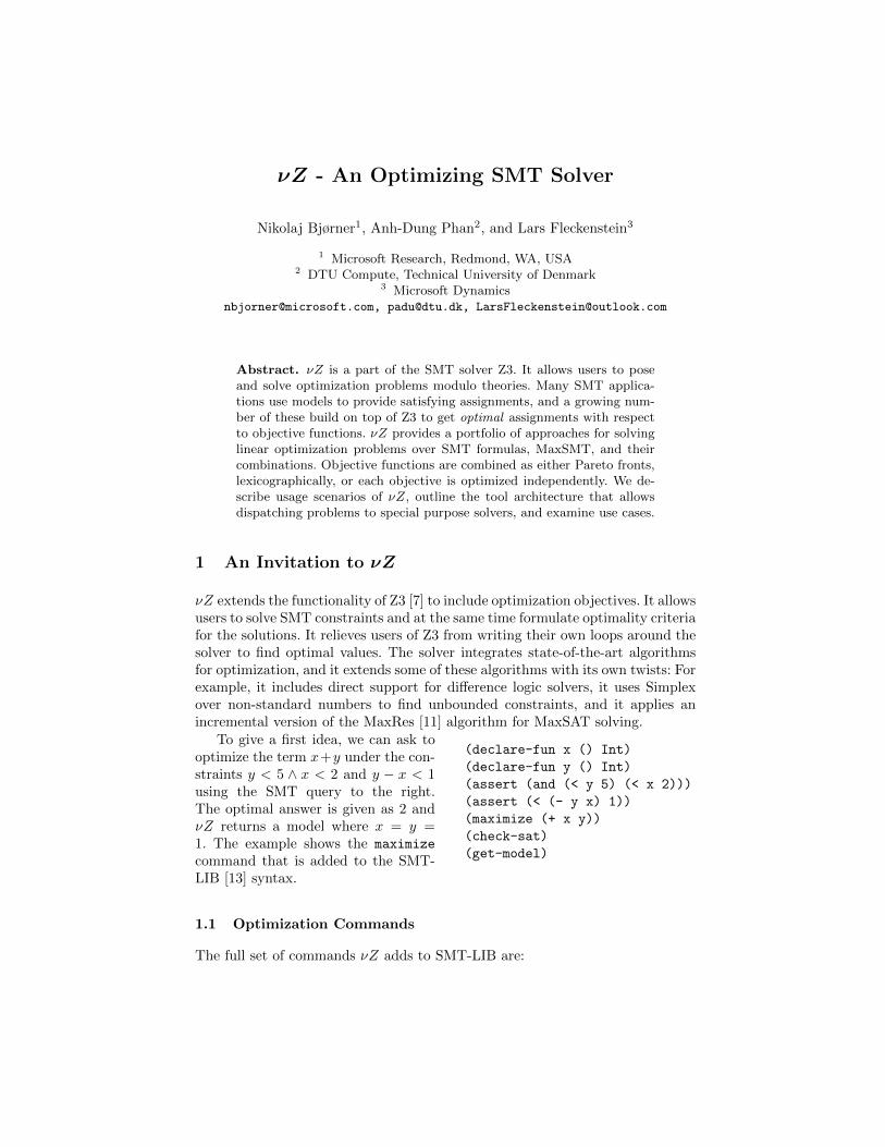
νZ - An Optimizing SMT Solver

Nikolaj Bjørner1, Anh-Dung Phan2, and Lars Fleckenstein3

1 Microsoft Research, Redmond, WA, USA2 DTU Compute, Technical University of Denmark

3 Microsoft Dynamicsnbjorner@microsoft.com, padu@dtu.dk, LarsFleckenstein@outlook.com

Abstract. νZ is a part of the SMT solver Z3. It allows users to poseand solve optimization problems modulo theories. Many SMT applica-tions use models to provide satisfying assignments, and a growing num-ber of these build on top of Z3 to get optimal assignments with respectto objective functions. νZ provides a portfolio of approaches for solvinglinear optimization problems over SMT formulas, MaxSMT, and theircombinations. Objective functions are combined as either Pareto fronts,lexicographically, or each objective is optimized independently. We de-scribe usage scenarios of νZ, outline the tool architecture that allowsdispatching problems to special purpose solvers, and examine use cases.

1 An Invitation to νZ

νZ extends the functionality of Z3 [7] to include optimization objectives. It allowsusers to solve SMT constraints and at the same time formulate optimality criteriafor the solutions. It relieves users of Z3 from writing their own loops around thesolver to find optimal values. The solver integrates state-of-the-art algorithmsfor optimization, and it extends some of these algorithms with its own twists: Forexample, it includes direct support for difference logic solvers, it uses Simplexover non-standard numbers to find unbounded constraints, and it applies anincremental version of the MaxRes [11] algorithm for MaxSAT solving.

(declare-fun x () Int)

(declare-fun y () Int)

(assert (and (< y 5) (< x 2)))

(assert (< (- y x) 1))

(maximize (+ x y))

(check-sat)

(get-model)

To give a first idea, we can ask tooptimize the term x+y under the con-straints y < 5 ∧ x < 2 and y − x < 1using the SMT query to the right.The optimal answer is given as 2 andνZ returns a model where x = y =1. The example shows the maximize

command that is added to the SMT-LIB [13] syntax.

1.1 Optimization Commands

The full set of commands νZ adds to SMT-LIB are:

(declare-fun x () Int)

(declare-fun y () Int)

(define-fun a1 () Bool (> x 0))

(define-fun a2 () Bool (< x y))

(assert (=> a2 a1))

(assert-soft a2 :dweight 3.1)

(assert-soft (not a1) :weight 5)

(check-sat)

(get-model)

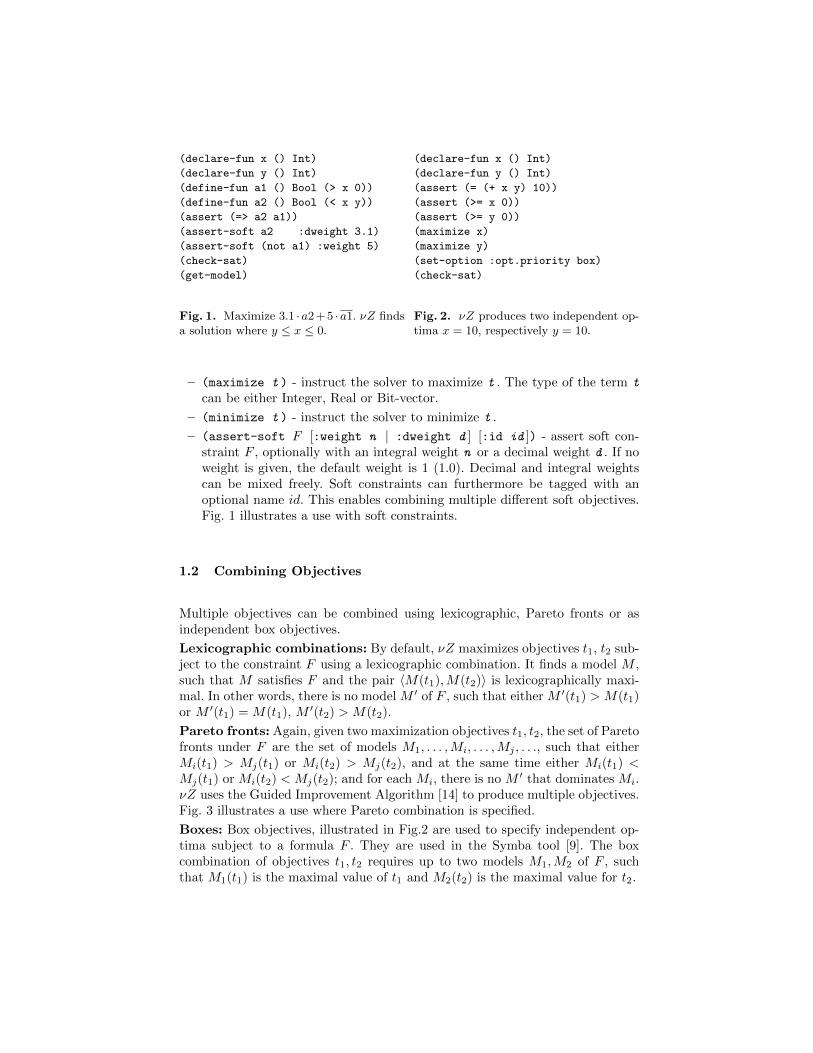
Fig. 1. Maximize 3.1 ·a2 + 5 ·a1. νZ findsa solution where y ≤ x ≤ 0.

(declare-fun x () Int)

(declare-fun y () Int)

(assert (= (+ x y) 10))

(assert (>= x 0))

(assert (>= y 0))

(maximize x)

(maximize y)

(set-option :opt.priority box)

(check-sat)

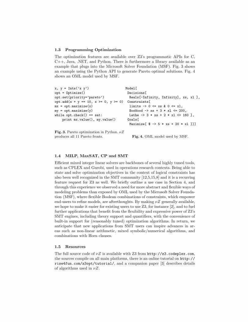
Fig. 2. νZ produces two independent op-tima x = 10, respectively y = 10.

– (maximize t ) - instruct the solver to maximize t . The type of the term t

can be either Integer, Real or Bit-vector.

– (minimize t ) - instruct the solver to minimize t .

– (assert-soft F [:weight n | :dweight d ] [:id id ]) - assert soft con-straint F , optionally with an integral weight n or a decimal weight d . If noweight is given, the default weight is 1 (1.0). Decimal and integral weightscan be mixed freely. Soft constraints can furthermore be tagged with anoptional name id. This enables combining multiple different soft objectives.Fig. 1 illustrates a use with soft constraints.

1.2 Combining Objectives

Multiple objectives can be combined using lexicographic, Pareto fronts or asindependent box objectives.

Lexicographic combinations: By default, νZ maximizes objectives t1, t2 sub-ject to the constraint F using a lexicographic combination. It finds a model M ,such that M satisfies F and the pair 〈M(t1),M(t2)〉 is lexicographically maxi-mal. In other words, there is no model M ′ of F , such that either M ′(t1) > M(t1)or M ′(t1) = M(t1), M ′(t2) > M(t2).

Pareto fronts: Again, given two maximization objectives t1, t2, the set of Paretofronts under F are the set of models M1, . . . ,Mi, . . . ,Mj , . . ., such that eitherMi(t1) > Mj(t1) or Mi(t2) > Mj(t2), and at the same time either Mi(t1) <Mj(t1) or Mi(t2) < Mj(t2); and for each Mi, there is no M ′ that dominates Mi.νZ uses the Guided Improvement Algorithm [14] to produce multiple objectives.Fig. 3 illustrates a use where Pareto combination is specified.

Boxes: Box objectives, illustrated in Fig.2 are used to specify independent op-tima subject to a formula F . They are used in the Symba tool [9]. The boxcombination of objectives t1, t2 requires up to two models M1,M2 of F , suchthat M1(t1) is the maximal value of t1 and M2(t2) is the maximal value for t2.

1.3 Programming Optimization

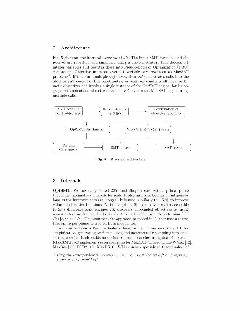
The optimization features are available over Z3’s programmatic APIs for C,C++, Java, .NET, and Python. There is furthermore a library available as anexample that plugs into the Microsoft Solver Foundation (MSF). Fig. 3 showsan example using the Python API to generate Pareto optimal solutions. Fig. 4shows an OML model used by MSF.

x, y = Ints(’x y’)

opt = Optimize()

opt.set(priority=’pareto’)

opt.add(x + y == 10, x >= 0, y >= 0)

mx = opt.maximize(x)

my = opt.maximize(y)

while opt.check() == sat:

print mx.value(), my.value()

Fig. 3. Pareto optimization in Python. νZproduces all 11 Pareto fronts.

Model[

Decisions[

Reals[-Infinity, Infinity], xs, xl ],

Constraints[

limits -> 0 <= xs & 0 <= xl,

BoxWood -> xs + 3 * xl <= 200,

Lathe -> 3 * xs + 2 * xl <= 160 ],

Goals[

Maximize[ $ -> 5 * xs + 20 * xl ]]]

Fig. 4. OML model used by MSF.

1.4 MILP, MaxSAT, CP and SMT

Efficient mixed integer linear solvers are backbones of several highly tuned tools,such as CPLEX and Gurobi, used in operations research contexts. Being able tostate and solve optimization objectives in the context of logical constraints hasalso been well recognized in the SMT community [12,5,15,8] and it is a recurringfeature request for Z3 as well. We briefly outline a use case in Section 4, andthrough this experience we observed a need for more abstract and flexible ways ofmodeling problems than exposed by OML used by the Microsoft Solver Founda-tion (MSF), where flexible Boolean combinations of constraints, which empowerend-users to refine models, are afterthoughts. By making νZ generally available,we hope to make it easier for existing users to use Z3, for instance [2], and to fuelfurther applications that benefit from the flexibility and expressive power of Z3’sSMT engines, including theory support and quantifiers, with the convenience ofbuilt-in support for (reasonably tuned) optimization algorithms. In return, weanticipate that new applications from SMT users can inspire advances in ar-eas such as non-linear arithmetic, mixed symbolic/numerical algorithms, andcombinations with Horn clauses.

1.5 Resources

The full source code of νZ is available with Z3 from http://z3.codeplex.com,the sources compile on all main platforms, there is an online tutorial on http://

rise4fun.com/z3opt/tutorial/, and a companion paper [3] describes detailsof algorithms used in νZ.

2 Architecture

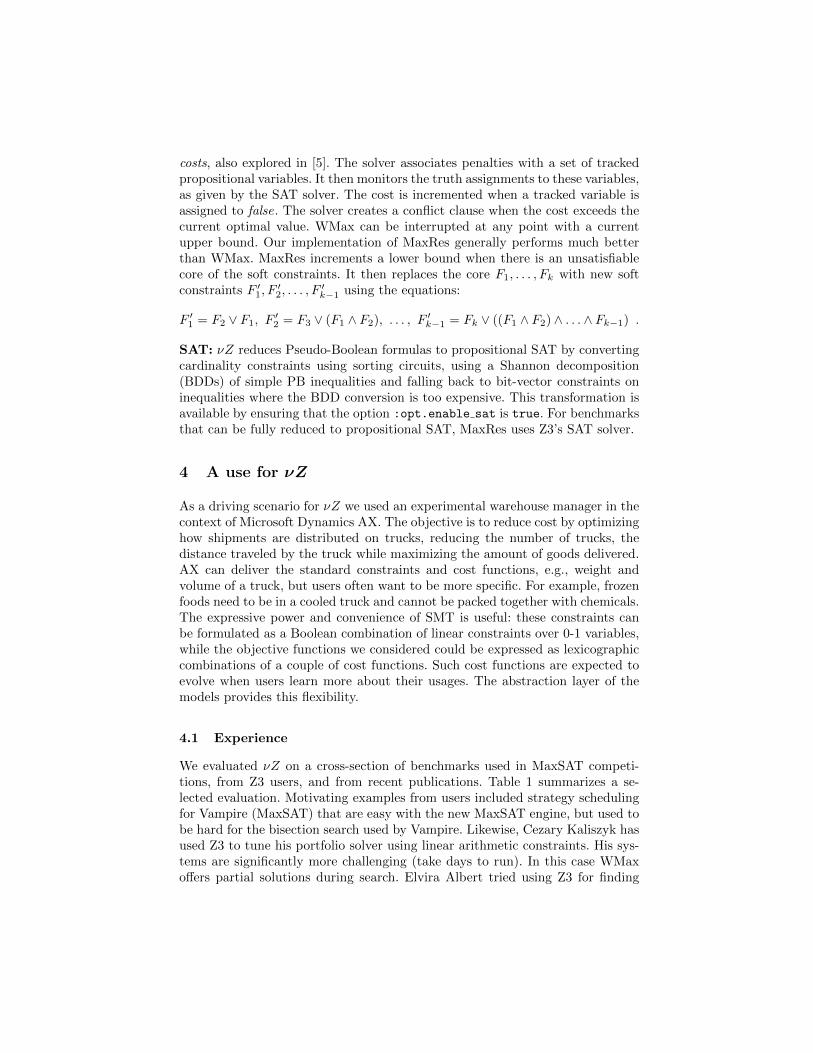
Fig. 5 gives an architectural overview of νZ. The input SMT formulas and ob-jectives are rewritten and simplified using a custom strategy that detects 0-1integer variables and rewrites these into Pseudo-Boolean Optimization (PBO)constraints. Objective functions over 0-1 variables are rewritten as MaxSATproblems4. If there are multiple objectives, then νZ orchestrates calls into theSMT or SAT cores. For box constraints over reals, νZ combines all linear arith-metic objectives and invokes a single instance of the OptSMT engine; for lexico-graphic combinations of soft constraints, νZ invokes the MaxSAT engine usingmultiple calls.

0-1 constraints⇒ PBO

SMT formulawith objectives

Combination ofobjective functions

OptSMT: Arithmetic MaxSMT: Soft Constraints

PB andCost solvers

SMT solver SAT solver

Fig. 5. νZ system architecture

3 Internals

OptSMT: We have augmented Z3’s dual Simplex core with a primal phasethat finds maximal assignments for reals. It also improves bounds on integers aslong as the improvements are integral. It is used, similarly to [15,9], to improvevalues of objective functions. A similar primal Simplex solver is also accessibleto Z3’s difference logic engines. νZ discovers unbounded objectives by usingnon-standard arithmetic: It checks if t ≥ ∞ is feasible, over the extension fieldR∪{ε,∞ := 1/ε}. This contrasts the approach proposed in [9] that uses a searchthrough hyper-planes extracted from inequalities.

νZ also contains a Pseudo-Boolean theory solver. It borrows from [4,1] forsimplification, generating conflict clauses, and incrementally compiling into smallsorting circuits. It also adds an option to prune branches using dual simplex.MaxSMT: νZ implements several engines for MaxSAT. These include WMax [12],MaxRes [11], BCD2 [10], MaxHS [6]. WMax uses a specialized theory solver of

4 using the correspondence: maximize c1 · x1 + c2 · x2 ≡ (assert-soft x1 :weight c1),(assert-soft x2 :weight c2)

costs, also explored in [5]. The solver associates penalties with a set of trackedpropositional variables. It then monitors the truth assignments to these variables,as given by the SAT solver. The cost is incremented when a tracked variable isassigned to false. The solver creates a conflict clause when the cost exceeds thecurrent optimal value. WMax can be interrupted at any point with a currentupper bound. Our implementation of MaxRes generally performs much betterthan WMax. MaxRes increments a lower bound when there is an unsatisfiablecore of the soft constraints. It then replaces the core F1, . . . , Fk with new softconstraints F ′1, F

′2, . . . , F

′k−1 using the equations:

F ′1 = F2 ∨ F1, F′2 = F3 ∨ (F1 ∧ F2), . . . , F ′k−1 = Fk ∨ ((F1 ∧ F2) ∧ . . . ∧ Fk−1) .

SAT: νZ reduces Pseudo-Boolean formulas to propositional SAT by convertingcardinality constraints using sorting circuits, using a Shannon decomposition(BDDs) of simple PB inequalities and falling back to bit-vector constraints oninequalities where the BDD conversion is too expensive. This transformation isavailable by ensuring that the option :opt.enable sat is true. For benchmarksthat can be fully reduced to propositional SAT, MaxRes uses Z3’s SAT solver.

4 A use for νZ

As a driving scenario for νZ we used an experimental warehouse manager in thecontext of Microsoft Dynamics AX. The objective is to reduce cost by optimizinghow shipments are distributed on trucks, reducing the number of trucks, thedistance traveled by the truck while maximizing the amount of goods delivered.AX can deliver the standard constraints and cost functions, e.g., weight andvolume of a truck, but users often want to be more specific. For example, frozenfoods need to be in a cooled truck and cannot be packed together with chemicals.The expressive power and convenience of SMT is useful: these constraints canbe formulated as a Boolean combination of linear constraints over 0-1 variables,while the objective functions we considered could be expressed as lexicographiccombinations of a couple of cost functions. Such cost functions are expected toevolve when users learn more about their usages. The abstraction layer of themodels provides this flexibility.

4.1 Experience

We evaluated νZ on a cross-section of benchmarks used in MaxSAT competi-tions, from Z3 users, and from recent publications. Table 1 summarizes a se-lected evaluation. Motivating examples from users included strategy schedulingfor Vampire (MaxSAT) that are easy with the new MaxSAT engine, but used tobe hard for the bisection search used by Vampire. Likewise, Cezary Kaliszyk hasused Z3 to tune his portfolio solver using linear arithmetic constraints. His sys-tems are significantly more challenging (take days to run). In this case WMaxoffers partial solutions during search. Elvira Albert tried using Z3 for finding

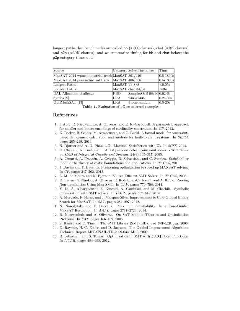
longest paths, her benchmarks are called bb (≈300 clauses), chat (≈3K clauses)and p2p (≈30K clauses), and we summarize timing for bb and chat below; thep2p category times out.

Source Category Solved instances Time

MaxSAT 2014 wpms industrial track MaxSAT 361/410 0.5-1800s

MaxSAT 2014 pms industrial track MaxSAT 406/568 0.5-1800s

Longest Paths MaxSAT bb 8/8 <0.05s

Longest Paths MaxSAT chat 34/34 1-36s

DAL Allocation challenge PBO SampleA&B 96/96 0.02-6s

Symba [9] LRA 2435/2435 0.2s-36s

OptiMathSAT [15] LRA 9 non-random 0.5-20sTable 1. Evaluation of νZ on selected examples

References

1. I. Abıo, R. Nieuwenhuis, A. Oliveras, and E. R.-Carbonell. A parametric approachfor smaller and better encodings of cardinality constraints. In CP, 2013.

2. K. Becker, B. Schatz, M. Armbruster, and C. Buckl. A formal model for constraint-based deployment calculation and analysis for fault-tolerant systems. In SEFM,pages 205–219, 2014.

3. N. Bjørner and A.-D. Phan. νZ - Maximal Satisfaction with Z3. In SCSS, 2014.4. D. Chai and A. Kuehlmann. A fast pseudo-boolean constraint solver. IEEE Trans.

on CAD of Integrated Circuits and Systems, 24(3):305–317, 2005.5. A. Cimatti, A. Franzen, A. Griggio, R. Sebastiani, and C. Stenico. Satisfiability

modulo the theory of costs: Foundations and applications. In TACAS, 2010.6. J. Davies and F. Bacchus. Postponing optimization to speed up MAXSAT solving.

In CP, pages 247–262, 2013.7. L. M. de Moura and N. Bjørner. Z3: An Efficient SMT Solver. In TACAS, 2008.8. D. Larraz, K. Nimkar, A. Oliveras, E. Rodrıguez-Carbonell, and A. Rubio. Proving

Non-termination Using Max-SMT. In CAV, pages 779–796, 2014.9. Y. Li, A. Albarghouthi, Z. Kincaid, A. Gurfinkel, and M. Chechik. Symbolic

optimization with SMT solvers. In POPL, pages 607–618, 2014.10. A. Morgado, F. Heras, and J. Marques-Silva. Improvements to Core-Guided Binary

Search for MaxSAT. In SAT, pages 284–297, 2012.11. N. Narodytska and F. Bacchus. Maximum Satisfiability Using Core-Guided

MaxSAT Resolution. In AAAI, pages 2717–2723, 2014.12. R. Nieuwenhuis and A. Oliveras. On SAT Modulo Theories and Optimization

Problems. In SAT, pages 156–169, 2006.13. S. Ranise and C. Tinelli. The SMT Library (SMT-LIB). www.SMT-LIB.org, 2006.14. D. Rayside, H.-C. Estler, and D. Jackson. The Guided Improvement Algorithm.

Technical Report MIT-CSAIL-TR-2009-033, MIT, 2009.15. R. Sebastiani and S. Tomasi. Optimization in SMT with LA(Q) Cost Functions.

In IJCAR, pages 484–498, 2012.

A Demonstration

We take a quick tour on available features in νZ. This section is based on theonline tutorial at http://rise4fun.com/Z3Opt/tutorial/guide. Please visitthe online playground for a quick try at νZ. More details of internals in νZ arealso available in a paper [3] that accompanies an invited talk at SCSS 2014. Thepaper describes, at a high level, the algorithms used for different optimizationstrategies in νZ.

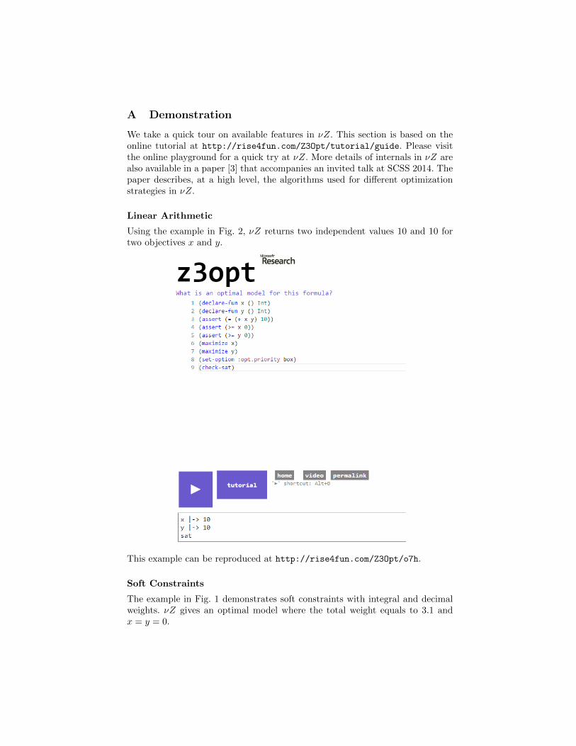
Linear Arithmetic

Using the example in Fig. 2, νZ returns two independent values 10 and 10 fortwo objectives x and y.

This example can be reproduced at http://rise4fun.com/Z3Opt/o7h.

Soft Constraints

The example in Fig. 1 demonstrates soft constraints with integral and decimalweights. νZ gives an optimal model where the total weight equals to 3.1 andx = y = 0.

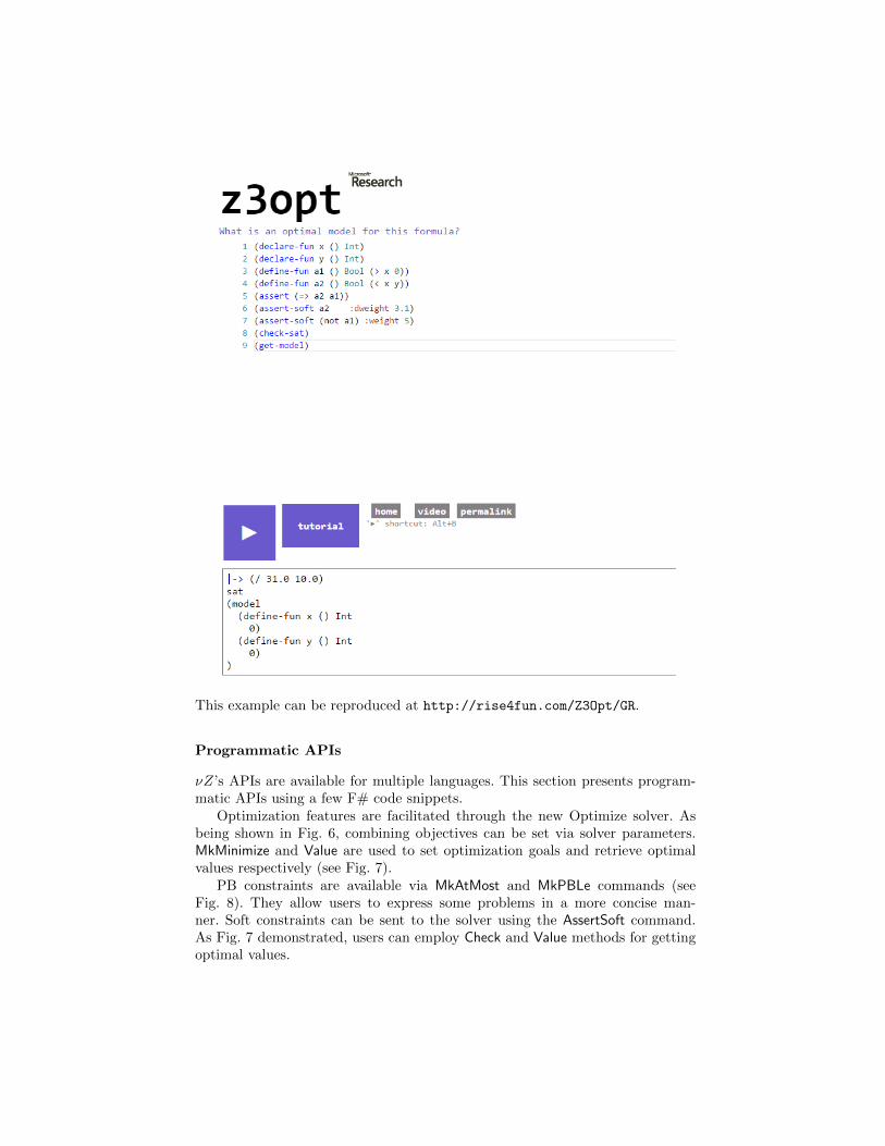
This example can be reproduced at http://rise4fun.com/Z3Opt/GR.

Programmatic APIs

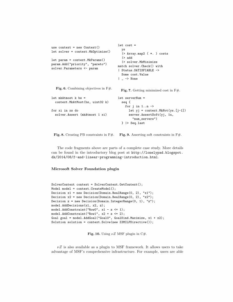
νZ’s APIs are available for multiple languages. This section presents program-matic APIs using a few F# code snippets.

Optimization features are facilitated through the new Optimize solver. Asbeing shown in Fig. 6, combining objectives can be set via solver parameters.MkMinimize and Value are used to set optimization goals and retrieve optimalvalues respectively (see Fig. 7).

PB constraints are available via MkAtMost and MkPBLe commands (seeFig. 8). They allow users to express some problems in a more concise man-ner. Soft constraints can be sent to the solver using the AssertSoft command.As Fig. 7 demonstrated, users can employ Check and Value methods for gettingoptimal values.

use context = new Context()

let solver = context.MkOptimize()

let param = context.MkParams()

param.Add("priority", "pareto")

solver.Parameters <- param

Fig. 6. Combining objectives in F#.

let cost =

ys

|> Array.map2 ( *. ) costs

|> add

|> solver.MkMinimize

match solver.Check() with

| Status.SATISFIABLE ->

Some cost.Value

| _ -> None

Fig. 7. Getting minimized cost in F#.

let mkAtmost k bs =

context.MkAtMost(bs, uint32 k)

for xi in xs do

solver.Assert (mkAtmost 1 xi)

Fig. 8. Creating PB constraints in F#.

let serverNum =

seq {

for j in 1..n ->

let yj = context.MkNot(ys.[j-1])

server.AssertSoft(yj, 1u,

"num_servers")

} |> Seq.last

Fig. 9. Asserting soft constraints in F#.

The code fragments above are parts of a complete case study. More detailscan be found in the introductory blog post at http://lonelypad.blogspot.

dk/2014/08/f-and-linear-programming-introduction.html.

Microsoft Solver Foundation plugin

SolverContext context = SolverContext.GetContext();

Model model = context.CreateModel();

Decision x1 = new Decision(Domain.RealRange(0, 2), "x1");

Decision x2 = new Decision(Domain.RealRange(0, 2), "x2");

Decision z = new Decision(Domain.IntegerRange(0, 1), "z");

model.AddDecisions(x1, x2, z);

model.AddConstraint("Row0", x1 - z <= 1);

model.AddConstraint("Row1", x2 + z <= 2);

Goal goal = model.AddGoal("Goal0", GoalKind.Maximize, x1 + x2);

Solution solution = context.Solve(new Z3MILPDirective());

Fig. 10. Using νZ MSF plugin in C#.

νZ is also available as a plugin to MSF framework. It allows users to takeadvantage of MSF’s comprehensive infrastructure. For example, users are able

to run multiple solvers in parallel with νZ inside MSF. The plugin plays a vitalrole in bootstrapping νZ by comparing it with other solvers in MSF.

Case study

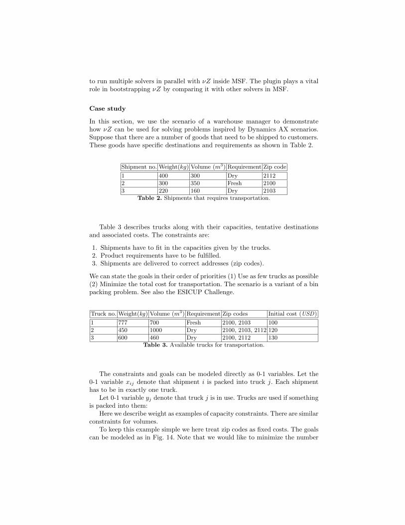
In this section, we use the scenario of a warehouse manager to demonstratehow νZ can be used for solving problems inspired by Dynamics AX scenarios.Suppose that there are a number of goods that need to be shipped to customers.These goods have specific destinations and requirements as shown in Table 2.

Shipment no. Weight(kg) Volume (m3) Requirement Zip code

1 400 300 Dry 2112

2 300 350 Fresh 2100

3 220 160 Dry 2103Table 2. Shipments that requires transportation.

Table 3 describes trucks along with their capacities, tentative destinationsand associated costs. The constraints are:

1. Shipments have to fit in the capacities given by the trucks.2. Product requirements have to be fulfilled.3. Shipments are delivered to correct addresses (zip codes).

We can state the goals in their order of priorities (1) Use as few trucks as possible(2) Minimize the total cost for transportation. The scenario is a variant of a binpacking problem. See also the ESICUP Challenge.

Truck no. Weight(kg) Volume (m3) Requirement Zip codes Initial cost (USD)

1 777 700 Fresh 2100, 2103 100

2 450 1000 Dry 2100, 2103, 2112 120

3 600 460 Dry 2100, 2112 130Table 3. Available trucks for transportation.

The constraints and goals can be modeled directly as 0-1 variables. Let the0-1 variable xij denote that shipment i is packed into truck j. Each shipmenthas to be in exactly one truck.

Let 0-1 variable yj denote that truck j is in use. Trucks are used if somethingis packed into them:

Here we describe weight as examples of capacity constraints. There are similarconstraints for volumes.

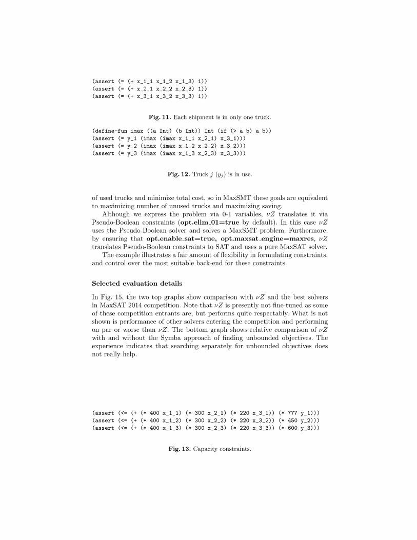
To keep this example simple we here treat zip codes as fixed costs. The goalscan be modeled as in Fig. 14. Note that we would like to minimize the number

(assert (= (+ x_1_1 x_1_2 x_1_3) 1))

(assert (= (+ x_2_1 x_2_2 x_2_3) 1))

(assert (= (+ x_3_1 x_3_2 x_3_3) 1))

Fig. 11. Each shipment is in only one truck.

(define-fun imax ((a Int) (b Int)) Int (if (> a b) a b))

(assert (= y_1 (imax (imax x_1_1 x_2_1) x_3_1)))

(assert (= y_2 (imax (imax x_1_2 x_2_2) x_3_2)))

(assert (= y_3 (imax (imax x_1_3 x_2_3) x_3_3)))

Fig. 12. Truck j (yj) is in use.

of used trucks and minimize total cost, so in MaxSMT these goals are equivalentto maximizing number of unused trucks and maximizing saving.

Although we express the problem via 0-1 variables, νZ translates it viaPseudo-Boolean constraints (opt.elim 01=true by default). In this case νZuses the Pseudo-Boolean solver and solves a MaxSMT problem. Furthermore,by ensuring that opt.enable sat=true, opt.maxsat engine=maxres, νZtranslates Pseudo-Boolean constraints to SAT and uses a pure MaxSAT solver.

The example illustrates a fair amount of flexibility in formulating constraints,and control over the most suitable back-end for these constraints.

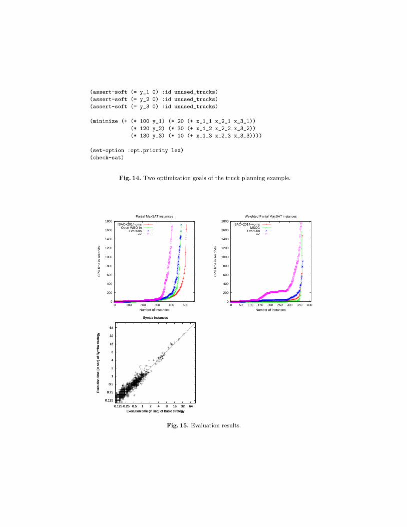
Selected evaluation details

In Fig. 15, the two top graphs show comparison with νZ and the best solversin MaxSAT 2014 competition. Note that νZ is presently not fine-tuned as someof these competition entrants are, but performs quite respectably. What is notshown is performance of other solvers entering the competition and performingon par or worse than νZ. The bottom graph shows relative comparison of νZwith and without the Symba approach of finding unbounded objectives. Theexperience indicates that searching separately for unbounded objectives doesnot really help.

(assert (<= (+ (* 400 x_1_1) (* 300 x_2_1) (* 220 x_3_1)) (* 777 y_1)))

(assert (<= (+ (* 400 x_1_2) (* 300 x_2_2) (* 220 x_3_2)) (* 450 y_2)))

(assert (<= (+ (* 400 x_1_3) (* 300 x_2_3) (* 220 x_3_3)) (* 600 y_3)))

Fig. 13. Capacity constraints.

(assert-soft (= y_1 0) :id unused_trucks)

(assert-soft (= y_2 0) :id unused_trucks)

(assert-soft (= y_3 0) :id unused_trucks)

(minimize (+ (* 100 y_1) (* 20 (+ x_1_1 x_2_1 x_3_1))

(* 120 y_2) (* 30 (+ x_1_2 x_2_2 x_3_2))

(* 130 y_3) (* 10 (+ x_1_3 x_2_3 x_3_3))))

(set-option :opt.priority lex)

(check-sat)

Fig. 14. Two optimization goals of the truck planning example.

0

200

400

600

800

1000

1200

1400

1600

1800

0 100 200 300 400 500

CP

U ti

me

in s

econ

ds

Number of instances

Partial MaxSAT instances

ISAC+2014-pmsOpen-WBO-In

Eva500aνZ

0

200

400

600

800

1000

1200

1400

1600

1800

0 50 100 150 200 250 300 350 400

CP

U ti

me

in s

econ

ds

Number of instances

Weighted Partial MaxSAT instances

ISAC+2014-wpmsMSCG

Eva500aνZ

0.125

0.25

0.5

1

2

4

8

16

32

64

0.125 0.25 0.5 1 2 4 8 16 32 64

Exe

cutio

n tim

e (in

sec

) of

Sym

ba s

trat

egy

Execution time (in sec) of Basic strategy

Symba instances

0.125

0.25

0.5

1

2

4

8

16

32

64

0.125 0.25 0.5 1 2 4 8 16 32 64

Exe

cutio

n tim

e (in

sec

) of

Sym

ba s

trat

egy

Execution time (in sec) of Basic strategy

Symba instances

Fig. 15. Evaluation results.