An O(m/ε3.5)-Cost Algorithm for Semidefinite Programs with

Diagonal Constraints

Yin Tat Lee∗ Swati Padmanabhan†

December 7, 2021

Abstract

We provide a first-order algorithm for semidefinite programs (SDPs) with diagonal constraints

on the matrix variable. Our algorithm outputs an ε-optimal solution with a run time of O(m/ε3.5),where m is the number of non-zero entries in the cost matrix. This improves upon the previousbest run time of O(m/ε4.5) by [AK07]. As a corollary of our result, given an instance of theMax-Cut problem with n vertices and m n edges, our algorithm returns a (1− ε)αGW cut in

the faster time of O(m/ε3.5), where αGW ≈ 0.878567 is the approximation ratio by [GW95]. Ourkey technical contribution is to combine an approximate variant of the Arora-Kale frameworkof mirror descent for SDPs with the idea of trading off exact computations in every iterationfor variance-reduced estimations in most iterations, only periodically resetting the accumulatederror with exact computations. This idea, along with the constructed estimator, are of possibleindependent interest for other problems that use the mirror descent framework.

1 Introduction

Consider the SDP maximizing C •X def= Tr(CX) over the set of n× n positive semidefinite matrices

with every diagonal entry bounded by a constant:

maxC •X subject to X 0, Xii ≤ 1 for all i ∈ [n]. (1.1)

We seek a matrix X∗ 0 with X∗ii ≤ 1 for all i ∈ [n] satisfying C • X∗ ≥ C •X∗− ε∑

i,j |Cij |, where

X∗ is an optimal solution of (1.1). This is not an ε-multiplicative guarantee (C •X∗ ≥ C •X∗(1−ε)),but a slightly weaker one, since

∑i,j |Cij | ≥ C •X∗. A multiplicative guarantee is not always easy

to provide; indeed, many classical optimization algorithms also provide a guarantee only additive insome quantity that bounds from above the difference of the function values between the initial andoptimal points. For example, gradient descent on an L-smooth convex function f over a set withdiameter D returns, after k iterations, a point xk such that f(xk) − f(x∗) ≤ O(LD2k−1), wheref(x0)− f(x∗) ≤ O(LD2).

To solve (1.1) as per the above accuracy criterion, it suffices to solve (1.2):

min f(X)def= −C •X +

n∑i=1

(Xii − ρi)+, subject to X 0. (1.2)

This problem is derived from (1.1) by promoting the diagonal constraints to the objective and

appropriately scaling C to Cdef= diag(1/

√ρ)C diag(1/

√ρ), where ρ ∈ Rn such that ρi =

∑j∈[n] |Cij |.

∗yintat@uw.edu. University of Washington.†pswati@uw.edu. University of Washington.

1

arX

iv:1

903.

0185

9v2

[cs

.DS]

6 D

ec 2

021

By rescaling Cij = nCij/∑

i,j |Cij |, we assume∑

i∈[n] ρi = n. Lemma 1.1 gives a solution of (1.1)from a solution of (1.2).

For (1.1), [AK07] have the previous best run time linear in mdef= nnz(C), the size of the input.

Though there exist algorithms with better dependence on ε, their dependence on n is superlinear,as we describe in Section 1.1. In this paper, we operate in the regime of moderate ε and large n,focusing on first-order methods.

[AK07] use the matrix multiplicative weights (MMW) update, which can be interpreted as mirrordescent in the nuclear norm1, using the negative entropy function, Φ(X) = X • logX, over the scaledsimplex, D = X : X 0,TrX = n, as the mirror map. Their iterates at iteration t are given by

X(t) = nexp(Y (t)

)Tr exp

(Y (t)

) , where Y (t) =

t−1∑s=1

−η∇f(X(s)), (1.3)

with step size η = O(ε) and gradient ∇f(M) = diag(1M≥ρ) − C. Computing this gradient entailsonly comparing the diagonal entries of the current iterate with a fixed vector. Therefore, the naıvecomputational cost of this method is dominated by Ω(nω) for the matrix exponentiation [PC99],prohibitively expensive for a large problem dimension. [AK07] circumvent this by approximatingthe diagonal entries of the matrix exponential. Therefore, their overall cost is composed of thefollowing three parts: (1) mirror descent requiring O(1/ε2) iterations to converge, (2) degree O(1/ε)Taylor approximation of the matrix exponential, each matrix-vector product costing O(m), and(3) O(1/ε2) random projections [JL84] to estimate the diagonal entries of the matrix exponential;combined, these give a run time of O(m/ε5), which, [AZL17] observe, can be sped up to O(m/ε4.5)by using Chebyshev (instead of Taylor) approximation of matrix exponentials (see [SV+14]).

Our contribution. In this work, we solve (1.1) with a run time of O(m/ε3.5), thus speeding upthe current best run time for this problem. Our result (formally stated in Theorem 2) is effectedby careful technical work that incorporates variance-reduced estimators and fast products of matrixexponentials with vectors into the Arora-Kale framework of mirror descent for SDPs. We use thegeneralized negative entropy, Φ(X) = X • log(X) − TrX, as our mirror map, and our primaryhigh-level idea is the following: instead of exactly computing the primal iterate in each iteration, wefrequently approximate it at a low accuracy (to reduce the cost) and infrequently at a high accuracy (to“reset” the error resulting from approximation). This idea is inspired by recent variance-reductionmethods [SSZ13, JZ13, DBLJ14, HL16, SLRB17]. The periodic high-accuracy computations andsmall bias and variance of estimators in the low-accuracy computations ensure sufficient closeness, inthe appropriate norm, of the estimated iterates to the true ones, which, by the convergence guaranteeof approximate mirror descent, leads to an ε-optimal solution. Making this variance-reduction workin the MMW setting requires several technical ideas, as follows.

We introduce the technical idea of expanding the domain of our mirror map by a polylogarithmicfactor. Due to the expanded domain and our choice of the mirror map, the gradient step of mirrordescent falls in the interior of this domain. The upshot of this is that the primal iterate is relatedto the dual via simply a matrix exponential, with no trace normalization as in Equation 1.3. Thus,the quantity for which we require an estimator is greatly simplified. Drawing on the observation of[AK07] that the gradient uses only the diagonal entries of the primal iterate, we build an estimator,with a small bias and variance, for the change in diagonal entries of the (dual) matrix exponen-tial. We also prove the strong convexity parameter of our mirror map on the expanded domain byconfecting classical results from convex analysis in a novel way. Due to the ubiquity of the MMWframework in optimization, efficient algorithms for SDPs, balanced separators, Ramanujan sparsi-

1The nuclear norm of a matrix X ∈ Rm×n is the sum of its singular values: ‖X‖nuc

def=

∑min(m,n)i=1 σi(X).

2

fiers, packing/covering, and machine learning, we anticipate that our technical contributions will beuseful for problems that hinge on the MMW foundation.

Applications. When C is a graph Laplacian, (1.1) is the SDP relaxation of the Max-Cut problem[GW95]. An NP-complete problem [Kar72], Max-Cut has seen widespread utility in circuit de-sign [CKC83], statistical physics [BGJR88], semi-supervised learning [WJC13], and phase recovery[WdM15]. Another instance of (1.1) is max-norm regularization [Jag11], a convex surrogate for rankminimization [SS05] enforcing simplicity in modeling observations [FHB04]. SDPs of the form of (1.1)have also found applications in community detection [ABH15, GV16, MS16a] and as relaxations tothe maximum-likelihood estimator in the group synchronization problem [SS11, BCSZ14].

1.1 Related work

We describe in this section previous work on (1.1) using first-order methods, other than that of[AK07]. Of note is that most papers below solve problems more general than (1.1), and the runtimes we mention occur when specialized to (1.1).

Saddle-point formulation. Since any SDP can be instantiated as an online convex optimizationproblem, we apply to our setting some notable results from this area. To do so, we first reduce (1.1) toa feasibility problem following the approach of [AHK05]. Recall our assumption that

∑i,j |Cij | = n.

The facts X∗ 0 and X∗ii ≤ 1 for i ∈ [n] imply |X∗ij |2 ≤ X∗iiX∗jj ≤ 1, which in turn bounds the

optimum from above as OPT =∑

i,j CijX∗ij ≤

∑i,j |Cij ||X∗ij | ≤ n. We can also bound the optimum

from below by choosing X to be the zero matrix, thus bounding OPT with λ ∈ [0, n]. Let A0 = 1λC,

b0 = 1, Ai = −eie>i , and bi = −1 for i ∈ [n]. Therefore, solving (1.1) requires, for each guess of λ(obtained via a binary search over its range), solving the feasibility problem:

Find Z ∈ Sn≥0 subject to Ai • Z − bi ≥ 0, for all i ∈ 0, n,TrZ ≤ n. (1.4)

To do so, we leverage the saddle-point problem studied by [GH16],

maxX∈Sn≥0,TrX=1

minp∈Rm

≥0,‖p‖1=1

m∑i=1

pi(Ai •X − bi). (1.5)

If the optimum of (1.5) is non-negative, solving it up to an additive accuracy of ε is equivalent tofinding a solution in the spectrahedron that satisfies all Ai •X − bi ≥ 0 upto an additive error of ε.For (1.4), this means the solution for (1.5) satisfies Xii ≈ 1/n± ε. However, due to the requirementof Xii ≈ 1 ± ε in (1.1), the accuracy parameter of (1.5) must be ε/n. This causes the run time of[GH16] for (1.1) to be O(m(n/ε)2.5). By the same reasoning, when solving (1.1) to ε multiplicativeaccuracy, the work of [BBN13], which uses a randomized Mirror-Prox algorithm, incurs a cost ofO(n5/ε3), and the recent algorithms of Follow the Compressed Leader by [AZL17] and rank-1 sketchby [CDST19] incur a cost of O(m(n/ε)2.5). It must be noted that [GH16], [AZL17], and [CDST19]provide algorithms satisfying ε-additive accuracy. When we translate our accuracy results to theirlanguage, the costs are not quite comparable. For instance, [CDST19], for ε-additive accuracy for(1.1), incurs a cost of m(n‖C‖∞/ε)2.5. Our algorithm, using this accuracy criterion, incurs a cost ofm(∑

i,j |Cij |/ε)3.5. Unless we assume additional structure on the matrix C, the comparison betweenthese two costs is inconclusive.

Low-rank updates. When C is the graph Laplacian in (1.1), there exists an ε-accurate solutionof rank O(1/ε) [RS09, MS16b, MMMO17]. Many papers capitalize on this fact and perform low-rank updates, which reduces cost per iteration. For example, [KL96] base their algorithm on theframework of [PST91] in conjunction with the power method to achieve a run time of O(mn/ε3). Asanother example, [Haz08] incorporates into the Frank-Wolfe algorithm [FW56] fast computation of

3

an approximate minimum eigenvector and provides an O(mn3/ε3)-algorithm. A recent noteworthyresult [YTF+19] returns a rank-R approximation to an ε-optimal solution at a cost O(R/ε2 +n/ε3).Even though, as alluded to earlier, there exists a rank-O(1/ε) solution to the MaxCut SDP, perturbingsuch a solution by an appropriately small amount gives an ε-optimal solution that is in fact full rank.Indeed, per Theorem 6.2 of [YTF+19], for any r < R, the iterate Xt returned by their algorithm initeration t satisfies lim supt→∞EΩ dist∗(Xt,Ψ∗) ≤ (1 + r/(R− r− 1)) ·maxX∈Ψ∗ ‖X − [X]r‖∗, whereΩ is the randomness in their algorithm, Ψ∗ is the solution set, R is the rank of the iterate returned,and [X]r is an r-truncated singular value decomposition of matrix X. The existence of full-rankmatrices in the solution set Ψ∗ implies a possibly large bound above, so one cannot conclude that[YTF+19] improves upon our run time.

Polynomial mirror map. One of the contributions of [AZL17] is a “polynomial-style” mirrormap such as Φ(X) = 1

1+1/2p TrX1+1/2p. The projection step with this map is X = (Y +)2p, where

Y + is the matrix obtained by zeroing out the negative eigenvalues of Y , which is as expensive asmatrix exponentiation.

Variance-reduction methods. Standard variance reduction algorithms such as SVRG [JZ13]minimize an objective that is a sum of functions, employing an unbiased estimator of the gradi-ent. Unfortunately, neither is (1.2) a sum of functions, nor is its gradient (diag(1X>=ρ)) cheap toestimate.

1.2 Preliminaries

Notation. We use Rn to denote the subspace of n-dimensional real vectors, 1 for the vector of allones, and 1E for the all-zero vector with one at coordinates where E is true. We use x+ to denote thenon-smooth function x when x ≥ 0 and zero otherwise. Denote by Sn the subspace of n×n symmetricmatrices and by In the n×n identity matrix. For u ∈ Rn, diag(u) is the n×n diagonal matrix with

diag(u)ii = ui. For A,B ∈ Sn, the trace inner product is A •B def= Tr(AB) =

∑i,j AijBij . We define

|||A||| =∑

i |Aii|. Given a scalar function f and a vector u, we use f(u) to mean that entrywise, andsimilarly, for a symmetric matrix A = UΛU>, f(A) = Uf(Λ)U>. Given A ∈ Rn×n and p ∈ Rn,

A ≥ p means Aii ≥ pi for all i ∈ [n]. For u ∈ Rn, N ∈ N, and vectors ζki.i.d.∼ N (0, In) for k ∈ [N ], the

scalar v = RandProj(u,N)def= 1

N

∑Nk=1(uT ζk)

2. This implies E v = ‖u‖22. We extend the definitionto A ∈ Sn with each row of A as the vector u. Then the diagonal matrix B = RandProj(A,N)satisfies EB = diagA2. We use O to denote polylogarithmic factors. The superscript ∗ denotesoptimality for variables and Fenchel conjugate for functions.

Fact 0.1 ([ALO16]). Given A 0, B ∈ Sn, and α ∈ [0, 1], the inequality Tr(BAαBA1−α) ≤ A •B2

holds.

Fact 0.2 ([Wil67]). For a symmetric matrix-valued function X(t) with argument scalar t, we haveddt exp(X(t)) =

∫ 1α=0 exp(αX(t)) ddtX(t) exp((1− α)X(t))dα.

Setup. Our underlying algorithm to solve (1.2) is a slight variant of lazy mirror descent (alsocalled Nesterov’s Dual Averaging [Nes09]), which we term approximate lazy mirror descent. To solveminx∈X f(x) using this algorithm, select a mirror map Φ : D → R and a norm; the associated

Bregman Divergence is DΦ(x, y)def= Φ(x) − Φ(y) − 〈∇Φ(y), x− y〉; set x(1) ∈ argminX∩D Φ(x) and

z(1) ∈ ∇−1Φ(0). We repeat, in succession, the gradient update, ∇Φ(z(t+1)) = ∇Φ(z(t))− η∇f(x(t)),and the approximate projection, finding x(t+1) satisfying E ‖x(t+1) − x(t+1)‖ ≤ δ, where x(t+1) ∈argminx∈X∩D DΦ(x, z(t+1)).

Theorem 1 (Convergence of Lazy Mirror Descent). Fix a norm ‖ · ‖. Given an α-strongly convexmirror map Φ : D → R and a convex, G-Lipschitz objective f : X → R, run Algorithm 3 with step

4

size η and E ‖x(t) − x(t)‖ ≤ δ. Let Ddef= supx∈X∩D Φ (x) − infx∈X∩D Φ (x). Then, Algorithm 3 after

T iterations returns xt∗, satisfying

E f(x(t∗))− f (x∗) ≤ D

Tη+

2ηG2

α+ δG. (1.6)

Lemma 1.1. Given C ∈ Rn×n and 0 X, let ρ ∈ Rn with ρi =∑n

j=1 |Cij |; diagonal matrix S with

Sii = min(1/√ρi, 1/√Xii) for i ∈ [n]; X = SXS; C = diag (1/√ρ)C diag(1/√ρ). Then, X 0, Xii ≤ 1

for all i ∈ [n], and C •X −∑n

i=1 (Xii − ρi)+ ≤ C • X.

2 Our approach

We present our algorithm below, parameters in Table 1, and main result in Theorem 2.

Algorithm 1 Our Algorithm

Input: Cost matrix C ∈ Rn×n, accuracy εParameters: Displayed in Table 1Initialize t← 0, Y (1) ← 0. Set C and ρ from Lemma 1.1 and ∇f(X) = diag(1X≥ρ)− Cfor Touter iterations do

t← t+ 1exp(1

2Y(t))← ChebyExp(1

2Y(t),TCheby, δCheby) . Defined in Corollary 2

X(t) ← RandProj(exp(12Y

(t)),Tjl) . High-accuracy projection

Y (t+1) ← Y (t) − η∇f(X(t)) . Gradient updatefor ti = 1→ Tinner do

t← t+ 1θ(ti) ← UpdateEstimator(X(t−1), Y (t−1), ε, η) . See Algorithm 2

X(t)jj ← (

√X

(t−1)jj + 1 + θ

(ti)j )2 − 1 for j ∈ [n] . Constant-accuracy projection

Y (t+1) ← Y (t) − η∇f(X(t)) . Gradient updateend

end

For t∗unif.∼ 1, 2, . . . , t, return Y (t∗) and S, where S is from Lemma 1.1.

Parameter Value Proof

Diameter D K logK Lemma 3.11Strong convexity α 1/(4K) Lemma 2.7

Step size η 18×104(log(n/ε))11 ε

2 Lemma 9.1

Inner iteration count Tinner ε−2 Section C.4Outer iteration count Touter

1ε · 24× 105(log(n/ε))11 log n Lemma 2.6

JL projection count Tjl (2× 105) · (log n)21 · ε−2 Lemma 9.1

Chebyshev approximation degree TCheby 150 log(n/ε) · ε−1/2 Lemma 8.2Chebyshev approximation accuracy δCheby (ε/n)401 Lemma 8.2

Table 1: All Algorithm 1 parameters and where their values are set. K = 40n(log n)10.

Theorem 2 (Main Result). Given C ∈ Rn×n with m ≥ n non-zero entries and 0 < ε ≤ 12 , we can

find, in time O(m/ε3.5) and with high probability, a matrix Y ∈ Sn with O (m) non-zero entries and

5

a diagonal matrix S ∈ Rn×n so that2 X∗def= S · expY · S satisfies X∗ 0, X∗ii ≤ 1 for i ∈ [n], and

C • X∗ ≥ C •X∗ − ε∑

i,j |Cij |.

As a corollary, for the Max-Cut problem on a graph with n nodes and m edges, our algorithm givesa cut that is (1 − ε)αGW optimal3, in time O(m/ε3.5), where αGW ≈ 0.878567. Before proceedingto the proof sketch of Theorem 2, we call attention to a technical concept crucial to our analysis:we add to (1.2) the constraint TrX ≤ K, where K = 40n(log n)10. The optimal X∗ remains validunder this constraint because TrX∗ = n. Throughout our algorithm, this inequality remains inactive(Lemma 2.6). Coupled with the Legendre dual of our mirror map Φ(X) = X • logX − TrX, thisresults in the primal and the dual being related by X = exp(Y ) (Lemma 9.2). Since the gradientrequires only diagonal entries of the primal iterate, we need estimators only for the diagonal entriesof exp(Y ).

Proof Sketch of Theorem 2. In this proof sketch, we compute the run time of Algorithm 1, provingthe claims in Theorem 2. In doing so, we provide intuition for the choice of parameters in Table 1.This sketch assumes that we are in iteration t and drops all superscripts, and aside from that, followsthe notation of Algorithm 1.

1. To compute exp(Y )ii, we first approximate exp(Y/2) to ε-accuracy using Chebyshev polynomials.

We show in Lemma 8.1 that the spectrum of Y lies in the range [−O(1/ε), O(1)], which allowsfor Chebyshev approximation with O(1/

√ε) terms, thus giving the cost of each projection to be

O(m/√ε). The upper bound of O(1) on the spectrum is critical to getting this cost, for in case

of a symmetric range of [−O(1/ε),O(1/ε)], the cost would be O(1/ε). The O(1/√ε) terms is

in contrast with the O(1/ε) required for Taylor approximation. We then estimate each exp(Y )iiwith O(1/ε2) projections via the JL sketch in the high-accuracy steps, and O(1) randomizedprojections in the Tinner low-accuracy steps. Therefore the total cost of the algorithm over Touter

iterations is roughly Touter · (m/√ε) · (1/ε2 + Tinner). From this expression, the optimal choice of

Tinner (up to polylogarithmic factors) is Tinner = 1/ε2.

2. Due to the small bias and variance of our estimator, after Tinner inner iterations, the estimatediterate is roughly within εK distance of the true iterate. Thus, the condition in Theorem 1is satisfied, and its the error bound applies at the end of our algorithm: E f(X∗) − f(X∗) ≤D/(Tη) + 2ηG2/α + δG. Using D, G, and α from Table 1 and Tinner from Step 1 and boundingby εK, this inequality simplifies to ε2/(ηTouter) + η ≤ ε.

3. The step size η is chosen by studying the error generated in each estimation step versus theerror our framework can tolerate. Estimating (exp(Y + ∆))ii from (expY )ii via a first-orderapproximation accrues an error of Tr(∆ expY ). Applying Holder’s inequality, the value of G,and the trace bound enforced by Lemma 2.6 yields Tr(∆ expY ) ≤ ηK. Therefore, after Tinner

iterations, the variance of the error is Tinnerη2K2. Equivalently, the overall error after Tinner

iterations is√TinnerηK. For this to be bounded by εK, we must have η ≤ ε/

√Tinner. Plugging in

Tinner from Step 1 gives the step size: η ≈ ε2.

4. The value of η from Step 3 and the inequality from Step 2 give Touter ≈ 1/ε. Plugging this valueof Touter above gives the overall algorithm cost O(m/ε3.5).

We boost our result to the high probability statement of Theorem 2 over multiple runs of thealgorithm. We sidestep the issue of storage cost of X∗ and cost of matrix-matrix products by

2Since X∗ can be dense, we represent it implicitly by only returning the matrices Y and S.3Assuming the Unique Games Conjecture, this is the best we can hope for Max-Cut [KKMO07].

6

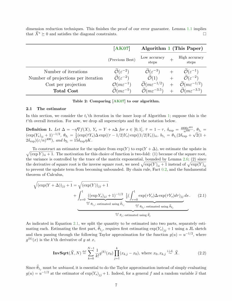
dimension reduction techniques. This finishes the proof of our error guarantee. Lemma 1.1 impliesthat X∗ 0 and satisfies the diagonal constraints.

[AK07] Algorithm 1 (This Paper)

(Previous Best)Low accuracy

steps+

High accuracysteps

Number of iterations O(ε−2) O(ε−3) + O(ε−1)

Number of projections per iteration O(ε−2) O(1) + O(ε−2)

Cost per projection O(mε−1) O(mε−1/2) + O(mε−1/2)

Total Cost O(mε−5) O(mε−3.5) + O(mε−3.5)

Table 2: Comparing [AK07] to our algorithm.

2.1 The estimator

In this section, we consider the ti’th iteration in the inner loop of Algorithm 1; suppose this is thet’th overall iteration. For now, we drop all superscripts and fix the notation below.

Definition 1. Let ∆ = −η∇f(X), Ys = Y + s∆ for s ∈ [0, 1], τ = 1 − τ , δexp = 4800ε401

n390 , θ1i =

(exp(Ys)ii + 1)−1/2, θ2i = 12(exp(τYs)∆ exp((τ − 1/2)Ys) exp((1/2)Ys))ii, b1i = θ1i(2δexp +

√2(1 +

2δexp)(ε/n)400), and b2i = 15δexpηK.

To construct an estimator for the update from exp(Y ) to exp(Y + ∆), we estimate the update in√(expY )ii + 1. The motivation for this choice of function is two-fold: (1) because of the square root,

the variance is controlled by the trace of the matrix exponential, bounded by Lemma 2.6; (2) sincethe derivative of square root is the inverse square root, we need

√exp(Y )ii + 1 instead of

√exp(Y )ii

to prevent the update term from becoming unbounded. By chain rule, Fact 0.2, and the fundamentaltheorem of Calculus,√

(exp(Y + ∆))jj + 1 =√

(exp(Y ))jj + 1

+

∫ 1

s=0((expYs)jj + 1)−1/2︸ ︷︷ ︸

def= θ1j ; estimated using θ1j

12(

∫ 1

τ=0exp(τYs)∆ exp(τYs)dτ)jj︸ ︷︷ ︸

def= θ2j ; estimated using θ2j

ds

︸ ︷︷ ︸def= θj ; estimated using θj

. (2.1)

As indicated in Equation 2.1, we split the quantity to be estimated into two parts, separately esti-mating each. Estimating the first part, θ1j , requires first estimating exp(Ys)jj + 1 using a JL sketch

and then passing through the following Taylor approximation for the function g(u) = u−1/2, whereg(k)(x) is the k’th derivative of g at x,

InvSqrt(X,N)def=

N−1∑k=0

1

k!g(k)(x0)

k∏j=1

(xk,j − x0), where x0, xk,ji.i.d.∼ X. (2.2)

Since θ1j must be unbiased, it is essential to do the Taylor approximation instead of simply evaluating

g(u) = u−1/2 at the estimator of exp(Ys)jj + 1. Indeed, for a general f and a random variable x that

7

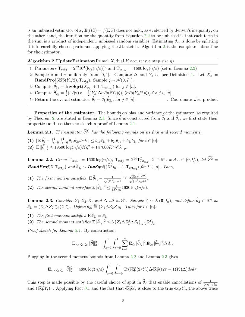
is an unbiased estimator of x, E f(x) = f(E x) does not hold, as evidenced by Jensen’s inequality; onthe other hand, the intuition for the quantity from Equation 2.2 to be unbiased is that each term inthe sum is a product of independent, unbiased random variables. Estimating θ2j is done by splittingit into carefully chosen parts and applying the JL sketch. Algorithm 2 is the complete subroutinefor the estimator.

Algorithm 2 UpdateEstimator(Primal X,dual Y, accuracy ε, step size η)

1: Parameters Testjl= 222104(log(n/ε))2 and Testisq = 1600 log(n/ε) (set in Lemma 2.2)

2: Sample s and τ uniformly from [0, 1]. Compute ∆ and Ys as per Definition 1. Let Xs =RandProj(exp(Ys/2),Testjl

). Sample ζ ∼ N (0, In).

3: Compute θ1j = InvSqrt(Xsjj + 1,Testisq) for j ∈ [n].

4: Compute θ2j = 12(exp((τ − 1

2)Ys)∆exp(τYs)ζ)j (exp(Ys/2)ζ)j for j ∈ [n].

5: Return the overall estimator, θj = θ1j θ2j , for j ∈ [n]. . Coordinate-wise product

Properties of the estimator. The bounds on bias and variance of the estimator, as requiredby Theorem 2, are stated in Lemma 2.1. Since θ is constructed from θ1 and θ2, we first state theirproperties and use them to sketch a proof of Lemma 2.1.

Lemma 2.1. The estimator θ(t) has the following bounds on its first and second moments.

(1) |E θi −∫ 1s=0

∫ 1τ=0 θ1iθ2idsdτ | ≤ b1iθ2i + b2iθ1i + b1ib2i for i ∈ [n].

(2) E ‖θ‖22 ≤ 19600 log(n/ε)Kη2 + 147000K2η2δexp.

Lemma 2.2. Given Testisq = 1600 log(n/ε), Testjl= 214T2

estisq, Z ∈ Sn, and ε ∈ (0, 1/2), let Z2 =

RandProj(Z,Testjl) and θ1i ∼ InvSqrt((Z2)ii + 1,Testisq) for i ∈ [n]. Then,

(1) The first moment satisfies

∣∣∣∣E θ1i − 1√(Z2)ii+1

∣∣∣∣ ≤ √2(ε/n)400√(Z2)ii+1

.

(2) The second moment satisfies E |θ1i |2 ≤ 1(Z2)ii

1630 log(n/ε).

Lemma 2.3. Consider Z1, Z2, Z, and ∆ all in Sn. Sample ζ ∼ N (0, In), and define θ2 ∈ Rn as

θ2i = (Z1∆Z2ζ)i (Zζ)i. Define θ2idef= (Z1∆Z2Z)ii. Then for i ∈ [n]:

(1) The first moment satisfies E θ2i = θ2i

(2) The second moment satisfies E |θ2i |2 ≤ 3(Z1∆Z2

2∆Z1

)ii

(Z2)ii

.

Proof sketch for Lemma 2.1. By construction,

Es,τ,ζ1,ζ2 ‖θ‖22 =

∫ 1

s=0

∫ 1

τ=0

n∑i=1

Eζ1 |θ1i |2 Eζ2 |θ2i |2dsdτ.

Plugging in the second moment bounds from Lemma 2.2 and Lemma 2.3 gives

Es,τ,ζ1,ζ2 ‖θ‖22 = 4890 log(n/ε)

∫ 1

s=0

∫ 1

τ=0Tr(exp(2τYs)∆exp((2τ − 1)Ys)∆)dsdτ.

This step is made possible by the careful choice of split in θ2 that enable cancellations of 1(expYs)ii

and (expYs)ii. Applying Fact 0.1 and the fact that expYs is close to the true expYs, the above trace

8

term is bounded by Tr(exp(Y + s∆)∆2

)(plus a small error term). Applying Holder’s Inequality,

Lemma 2.6, and values of η and G completes the proof.

To provide proof sketches of Lemma 2.2 and Lemma 2.3, we need two technical lemmas aboutRandProj and InvSqrt, the main workhorses for our estimators. These lemmas follow from prop-erties of Gaussian and the scaled chi-squared distribution.

Lemma 2.4. Consider a positive random variable x sampled from a distribution X with mean µand variance σ2. For some integer k > 0, construct the distribution G(X) = InvSqrt (X, k) definedin Equation 2.2. Then the random variable g ∼ G(X) satisfies

(1) |E g − µ−1/2| ≤ E(

|x−µ|k

min(µ,x)k+1/2

)(2) E |g|2 ≤ k

∑k−1j=0 E

((σ2+(µ−x)2)

j

x2j+1

).

Lemma 2.5. Given u ∈ Rn such that µdef= ‖u‖22 6= 0, and positive integers k > 1 and N ≥ 4k + 6,

the following are true for x sampled from X = RandProj (u,N).

(1) Ex = µ

(2) σ2 def= E (x− µ)2 = 2µ2

N

(3) E

((σ2+(x−µ)2)

k

min(x,µ)2k+1

)≤ 1

µ

(eN/2

2N−17k + 213kk2k

Nk

)Proof sketches of Lemmas 2.2 and 2.3. Consider x ∼ Z2

ii. By Lemma 2.5, Ex = Z2ii. This satisfies

the bias requirement of Lemma 2.4, and therefore∣∣∣∣∣E θ1i −1√

1 + (Z2)ii

∣∣∣∣∣ ≤ E

∣∣x− (Z2)ii∣∣Testisq

min(x+ 1, (Z2)ii + 1)Testisq+12

≤

√E

(x− (Z2)ii)2Testisq

min (x+ 1, (Z2)ii + 1)2Testisq+1

≤

√√√√ 1

(Z2)ii + 1

(eTestisq/2

2Testjl−17Testisq

+213Testisq Testisq

2Testisq

Testjl

Testisq

).

where the first step is by Lemma 2.4, the second is by Jensen’s inequality, and the third step is bya slight modification of (3) in Lemma 2.5. The values of Testisq and Testjl

from Algorithm 2 give the

final bias bound. The second moment bound follows similarly, and the properties of θ2 follow fromsimple properties of the Gaussian distribution.

2.2 Technical Concepts: Domain Expansion and Strong Convexity

In this section we state and sketch the proofs of two key technical concepts: (1) the addition of thetrace constraint as described before the proof of Theorem 2, and (2) the value of the strong convexityparameter of our mirror map over this new domain.

Lemma 2.6. With the choice of parameters in Algorithm 1, the iterate X(t) at any iteration tsatisfies Tr X(t) < K for K = 40n(log n)10.

9

Proof sketch. We assume that for any iteration t, the primal iterate is close to the optimal point andsatisfies |||X(t) −X∗||| ≤ 38n (log n)10. In Algorithm 1, Y (1) = 0 implies X(1) = I. We also know thatthe optimal point satisfies TrX∗ = n. Therefore, in the base case, |||X(1) −X∗||| ≤ 2n ≤ 38n (log n)10.Suppose that the hypothesis is true for some t = t′. We complete the proof by first proving a weakbound for |||X(t) −X∗||| using the triangle inequality of norms and then boosting our bound (therebyobtaining the stronger guarantee of the induction hypothesis) by invoking the strong convexity ofthe Bregman divergence. The full proof is presented in Section C.6.

We now sketch the proof of the strong convexity parameter of our mirror map, the generalizednegative entropy function. This mirror map is different from the negative entropy function and hasrecently appeared in [AO15].

Lemma 2.7. The function Φ(X) = X•logX−TrX is 14K -strongly convex with respect to the nuclear

norm over the domain D = X : X 0,TrX ≤ K.

Proof sketch. We invoke the duality between strong convexity and smoothness by [KST09], thecharacterization of matrix smooth functions by [JN08], and the generalization of convexity of apermutation-invariant function on vectors to a spectral function on matrices by [Lew95]. Our proofrequires the following definition.

Definition 2. Define the vector functions ψ1(y) =∑n

i=1 exp yi, ψ2(y) = 2K logψ1(y)−2K log(2K)+2K, ψ(y) = ψ1(y) if ψ1(y) ≤ 2K and ψ2(y) otherwise; Ψ(Y ) = Ψ1(Y ) if Ψ1(Y ) ≤ 2K and Ψ2(Y )otherwise; and φ(x) =

∑ni=1 xi log xi−

∑ni=1 xi. Define the corresponding matrix functions Ψ1(Y ) =

Tr expY , Ψ2(Y ) = 2K log Ψ1(Y )− 2K log(2K) + 2K, and Φ(X) = X • logX − TrX.

Our first step is to show that Ψ, the matrix version of ψ, satisfies the property Ψ∗(Y ) = Φ(Y )over Y : Y 0,TrY ≤ K. To prove this, we first prove that ψ and its matrix version, Ψ, areboth continuously differentiable at the boundary of definition of their respective two parts. We thenshow that ψ1 and ψ2 are convex; combining this with the claim about continuous differentiabilityimplies convexity of ψ, which immediately extends to Ψ by a result of [Lew95]. We then show thatψ and φ satisfy ψ∗1(x) = φ(x) for x ∈ Rn+, and given an input x ∈ x : xi ≥ 0,

∑ni=1 xi ≤ K, the

point y attaining the optimum in computing ψ∗1(x) lies in the interior of the set y : ψ1(y) ≤ 2K.Therefore, given an input x ∈ x : xi ≥ 0,

∑ni=1 xi ≤ K, we invoke the preceeding facts to conclude

that the point at which the value of ψ∗(x) is attained must be the same as that for ψ∗1(x). Thisimplies ψ∗(x) = ψ∗1(x) for x ∈ x : xi ≥ 0,

∑ni=1 xi ≤ K. By a result of [Lew95], this extends to

Ψ∗ = Φ on X : X 0,TrX ≤ K. We then use [JN08] and continuous differentiability at theboundary to show that Ψ is 4K-smooth in the operator norm which in turn implies, by [KST09],that Ψ∗ is 1/(4K)-strongly convex in the nuclear norm, finishing the proof. Our full proof is inSection C.1.

Acknowledgment

We are very grateful to the anonymous reviewers of SODA 2019, SODA 2020, and COLT 2020for their careful reading and constructive suggestions on improving our presentation, Kevin Tian(Stanford) for helpful explanations of his paper [CDST19], and Sidhanth Mohanty (UC Berkeley)for his clear explanation of bounds on the rank of the MaxCut SDP from [RS09] and [MS16b].

10

References

[ABH15] Emmanuel Abbe, Afonso S Bandeira, and Georgina Hall. Exact recovery in the stochas-tic block model. IEEE Transactions on Information Theory, 62(1):471–487, 2015. 1

[AHK05] Sanjeev Arora, Elad Hazan, and Satyen Kale. Fast algorithms for approximate semidefi-nite programming using the multiplicative weights update method. In 46th Annual IEEESymposium on Foundations of Computer Science (FOCS’05), pages 339–348. IEEE,2005. 1.1

[AK07] Sanjeev Arora and Satyen Kale. A combinatorial, primal-dual approach to semidefiniteprograms. In Proceedings of the thirty-ninth annual ACM symposium on Theory ofcomputing, pages 227–236, 2007. (document), 1, 1.1, ??, 2, 2.2, 3, 4

[ALO16] Zeyuan Allen Zhu, Yin Tat Lee, and Lorenzo Orecchia. Using optimization to obtaina width-independent, parallel, simpler, and faster positive SDP solver. In Proceedingsof the Twenty-Seventh Annual ACM-SIAM Symposium on Discrete Algorithms, SODA2016, Arlington, VA, USA, January 10-12, 2016, pages 1824–1831, 2016. 0.1

[AO15] Zeyuan Allen-Zhu and Lorenzo Orecchia. Using optimization to break the epsilon bar-rier: A faster and simpler width-independent algorithm for solving positive linear pro-grams in parallel. In Proceedings of the Twenty-Sixth Annual ACM-SIAM Symposiumon Discrete Algorithms, SODA ’15, 2015. 2.2

[AZL17] Zeyuan Allen-Zhu and Yuanzhi Li. Follow the compressed leader: faster online learningof eigenvectors and faster mmwu. In Proceedings of the 34th International Conferenceon Machine Learning-Volume 70, pages 116–125, 2017. 1, 1.1

[B+15] Sebastien Bubeck et al. Convex optimization: Algorithms and complexity. Foundationsand Trends® in Machine Learning, 8(3-4):231–357, 2015. A.2, C.6

[BBN13] Michel Baes, Michael Burgisser, and Arkadi Nemirovski. A randomized mirror-proxmethod for solving structured large-scale matrix saddle-point problems. SIAM Journalon Optimization, 23(2):934–962, 2013. 1.1

[BCSZ14] Afonso S Bandeira, Moses Charikar, Amit Singer, and Andy Zhu. Multireference align-ment using semidefinite programming. In Proceedings of the 5th conference on Innova-tions in theoretical computer science, pages 459–470, 2014. 1

[BGJR88] Francisco Barahona, Martin Grotschel, Michael Junger, and Gerhard Reinelt. An ap-plication of combinatorial optimization to statistical physics and circuit layout design.Operations Research, 36(3):493–513, 1988. 1

[BV04] Stephen Boyd and Lieven Vandenberghe. Convex Optimization. Cambridge UniversityPress, New York, NY, USA, 2004. C.1

[CDST19] Yair Carmon, John C. Duchi, Aaron Sidford, and Kevin Tian. A rank-1 sketch formatrix multiplicative weights. In Conference on Learning Theory, COLT 2019, 25-28June 2019, Phoenix, AZ, USA, pages 589–623, 2019. 1.1, 2.2

[CKC83] Ruen-Wu Chen, Yoji Kajitani, and Shu-Park Chan. A graph-theoretic via minimizationalgorithm for two-layer printed circuit boards. IEEE Transactions on Circuits andSystems, 30(5):284–299, 1983. 1

11

[DBLJ14] Aaron Defazio, Francis Bach, and Simon Lacoste-Julien. Saga: A fast incremental gra-dient method with support for non-strongly convex composite objectives. In Z. Ghahra-mani, M. Welling, C. Cortes, N. D. Lawrence, and K. Q. Weinberger, editors, Advancesin Neural Information Processing Systems 27, pages 1646–1654. 2014. 1

[FHB04] M. Fazel, H. Hindi, and S. Boyd. Rank minimization and applications in system theory.In Proceedings of the 2004 American Control Conference, 2004. 1

[FW56] M. Frank and P. Wolfe. An algorithm for quadratic programming. Naval researchlogistics quarterly, 3(1-2):95–110, 1956. 1.1

[GH16] Dan Garber and Elad Hazan. Sublinear time algorithms for approximate semidefiniteprogramming. Mathematical Programming, 158(1-2):329–361, 2016. 1.1

[GV16] Olivier Guedon and Roman Vershynin. Community detection in sparse networks viagrothendieck’s inequality. Probability Theory and Related Fields, 165(3-4):1025–1049,2016. 1

[GW95] Michel X Goemans and David P Williamson. Improved approximation algorithms formaximum cut and satisfiability problems using semidefinite programming. Journal ofthe ACM (JACM), 42(6):1115–1145, 1995. (document), 1

[Haz08] Elad Hazan. Sparse approximate solutions to semidefinite programs. In Latin Americansymposium on theoretical informatics, pages 306–316, 2008. 1.1

[HL16] Elad Hazan and Haipeng Luo. Variance-reduced and projection-free stochastic optimiza-tion. In Proceedings of the 33rd International Conference on International Conferenceon Machine Learning - Volume 48, ICML’16, 2016. 1

[Jag11] Martin Jaggi. Sparse Convex Optimization Methods for Machine Learning. PhD thesis,ETH Zurich, 2011. 1

[JL84] William B Johnson and Joram Lindenstrauss. Extensions of lipschitz mappings into ahilbert space. Contemporary mathematics, 26(189-206):1, 1984. 1, 3.9

[JN08] Anatoli Juditsky and Arkadii S Nemirovski. Large deviations of vector-valued mar-tingales in 2-smooth normed spaces. arXiv preprint arXiv:0809.0813, 2008. 2.2, 2.2,5

[JZ13] Rie Johnson and Tong Zhang. Accelerating stochastic gradient descent using predictivevariance reduction. In Advances in neural information processing systems, pages 315–323, 2013. 1, 1.1

[Kar72] R. Karp. Reducibility among combinatorial problems. In Complexity of ComputerComputations, pages 85–103. Plenum Press, 1972. 1

[KKMO07] Subhash Khot, Guy Kindler, Elchanan Mossel, and Ryan O’Donnell. Optimal inap-proximability results for max-cut and other 2-variable csps? 2007. 3

[KL96] Philip Klein and Hsueh-I Lu. Efficient approximation algorithms for semidefinite pro-grams arising from max cut and coloring. In Proceedings of the Twenty-eighth AnnualACM Symposium on Theory of Computing, STOC ’96, 1996. 1.1

12

[KST09] Sham M. Kakade, Shai Shalev-Shwartz, and Ambuj Tewari. Applications of strongconvexity–strong smoothness duality to learning with matrices. CoRR, abs/0910.0610,2009. 2.2, 2.2, 3.3, 4

[Lew95] Adrian S Lewis. The convex analysis of unitarily invariant matrix functions. Journal ofConvex Analysis, 2(1):173–183, 1995. 2.2, 2.2, 6

[LV07] Laszlo Lovasz and Santosh Vempala. The geometry of logconcave functions and samplingalgorithms. Random Structures & Algorithms, 30(3):307–358, 2007. 9

[MMMO17] Song Mei, Theodor Misiakiewicz, Andrea Montanari, and Roberto Imbuzeiro Oliveira.Solving sdps for synchronization and maxcut problems via the grothendieck inequality.In Conference on Learning Theory, COLT 2017, pages 1476–1515, 2017. 1.1

[MS16a] Andrea Montanari and Subhabrata Sen. Semidefinite programs on sparse random graphsand their application to community detection. In Proceedings of the forty-eighth annualACM symposium on Theory of Computing, pages 814–827, 2016. 1

[MS16b] Andrea Montanari and Subhabrata Sen. Semidefinite programs on sparse random graphsand their application to community detection. In Proceedings of the Forty-eighth AnnualACM Symposium on Theory of Computing, STOC ’16, 2016. 1.1, 2.2

[Nes09] Yurii Nesterov. Primal-dual subgradient methods for convex problems. Mathematicalprogramming, 120(1):221–259, 2009. 1.2

[PC99] Victor Y. Pan and Zhao Q. Chen. The complexity of the matrix eigenproblem. InProceedings of the Thirty-First Annual ACM Symposium on Theory of Computing, May1-4, 1999, Atlanta, Georgia, USA, pages 507–516, 1999. 1

[PST91] S. A. Plotkin, D. B. Shmoys, and E. Tardos. Fast approximation algorithms for frac-tional packing and covering problems. In [1991] Proceedings 32nd Annual Symposiumof Foundations of Computer Science, 1991. 1.1

[RS09] Prasad Raghavendra and David Steurer. How to round any csp. In Proceedings of the2009 50th Annual IEEE Symposium on Foundations of Computer Science, FOCS ’09,2009. 1.1, 2.2

[SLRB17] Mark Schmidt, Nicolas Le Roux, and Francis Bach. Minimizing finite sums with thestochastic average gradient. Mathematical Programming, 162(1-2):83–112, 2017. 1

[SS05] Nathan Srebro and Adi Shraibman. Rank, trace-norm and max-norm. In InternationalConference on Computational Learning Theory, pages 545–560, 2005. 1

[SS11] Amit Singer and Yoel Shkolnisky. Three-dimensional structure determination fromcommon lines in cryo-em by eigenvectors and semidefinite programming. SIAM journalon imaging sciences, 4(2):543–572, 2011. 1

[SSZ13] Shai Shalev-Shwartz and Tong Zhang. Stochastic dual coordinate ascent methods forregularized loss minimization. Journal of Machine Learning Research, 14(Feb):567–599,2013. 1

[SV+14] Sushant Sachdeva, Nisheeth K Vishnoi, et al. Faster algorithms via approximationtheory. Foundations and Trends® in Theoretical Computer Science, 9(2):125–210, 2014.1, C.2, 7, 7.1, 8

13

[WdM15] Irene Waldspurger, Alexandre d’Aspremont, and Stephane Mallat. Phase recovery,maxcut and complex semidefinite programming. Mathematical Programming, 2015. 1

[Wil67] R. M. Wilcox. Exponential Operators and Parameter Differentiation in QuantumPhysics. Journal of Mathematical Physics, 1967. 0.2

[WJC13] Jun Wang, Tony Jebara, and Shih-Fu Chang. Semi-supervised learning using greedymax-cut. Journal of Machine Learning Research, 14(Mar):771–800, 2013. 1

[YTF+19] Alp Yurtsever, Joel A. Tropp, Olivier Fercoq, Madeleine Udell, and Volkan Cevher.Scalable semidefinite programming, 2019. 1.1

14

Appendices

We organize the appendix into four parts: Section A, analysis common to [AK07] and us; Section Band Section C, analysis of [AK07] and our algorithm, respectively; Section D, general technicalresults.

A Analysis Common to Both Algorithms

In this section we provide proofs for two results: the first is that a solution to the reformulatedproblem (1.2) is indeed ε close to that of the original; the second is the convergence guarantee ofapproximate lazy mirror descent, the framework for both the Arora-Kale algorithm as well as ours.

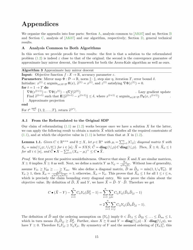
Algorithm 3 Approximate lazy mirror descent

Input: Objective function f : X → R, accuracy parameter ε.Parameters: Mirror map Φ : D → R, norm ‖ · ‖, step size η, iteration T , error bound δ.Initialize: x(1) ∈ argminx∈X∩D Φ(x), x(1) = x(1), and z(1) satisfying ∇Φ(z(1)) = 0.for t = 1→ T do

∇Φ(z(t+1))← ∇Φ(z(t))− η∇f(x(t)) . Lazy gradient updateFind x(t+1) such that E ‖x(t+1) − x(t+1)‖ ≤ δ, where x(t+1) ∈ argminx∈X∩D DΦ(x, z(t+1)) .Approximate projection

end

For t∗unif.∼ 1, 2, . . . , T, return x(t∗).

A.1 From the Reformulated to the Original SDP

Our claim of reformulating (1.1) as (1.2) works because once we have a solution X for the latter,we can apply the following result to obtain a matrix X which satisfies all the required constraints of(1.1), and at which the objective value in (1.1) is better than that at X in (1.2).

Lemma 1.1. Given C ∈ Rn×n and 0 X, let ρ ∈ Rn with ρi =∑n

j=1 |Cij |; diagonal matrix S with

Sii = min(1/√ρi, 1/√Xii) for i ∈ [n]; X = SXS; C = diag (1/√ρ)C diag(1/√ρ). Then, X 0, Xii ≤ 1

for all i ∈ [n], and C •X −∑n

i=1 (Xii − ρi)+ ≤ C • X.

Proof. We first prove the positive semidefiniteness. Observe that since X and X are similar matrices,X 0 implies X 0 as well. Next, we define a matrix Y as Yij =

Xij√ρi√ρj

. Without loss of generality,

assume Y11 ≥ Y22 ≥ . . . ≥ Ynn. We also define a diagonal matrix, D as Dii = min(1, 1/√Yii). If

Yii ≥ 1, then Xii = ρiYii√ρiYii

√ρiYii

= 1; otherwise, Xii = Yii. This proves that Xii ≤ 1 for all 1 ≤ i ≤ n,

which is precisely the claim bounding every diagonal entry. We now prove the claim about theobjective value. By definition of D, X and Y , we have X = D · Y · D. Therefore we get

C • (X − Y )−n∑i=1

CiiYii(D2ii − 1) =

n∑i=1

∑j 6=i

CijYij(DiiDjj − 1)

= 2

n∑i=1

∑i<j

CijYij(DiiDjj − 1).

The definition of D and the ordering assumption on Yii imply 0 < D11 ≤ D22 ≤ . . . ≤ Dnn ≤ 1,which in turn means DiiDjj ≥ D2

ii. Further, since X 0 and Y = diag(1/√ρ) ·X · diag(1/√ρ), wehave Y 0. Therefore YiiYjj ≥ YijYji. By symmetry of Y and the assumed ordering of Yiin1 , this

15

can be simplified to Yii ≥ |Yij | for i < j. These two facts simplify the above to

C • (X − Y )−n∑i=1

CiiYii(D2ii − 1) ≥ 2

n∑i=1

∑i<j

|Cij ||Yij |(D2ii − 1)

≥ 2

n∑i=1

∑i<j

|Cij |Yii(D2ii − 1)

Finally, since Dii ≤ 1, we have D2ii − 1 ≤ 0. Rearranging the terms in the last inequality, we get

C • (X − Y ) ≥n∑i=1

CiiYii(D2ii − 1) +

n∑i=1

Yii(D2ii − 1)(

∑j>i

|Cij |+∑j<i

|Cij |)

=n∑i=1

Yii(D2ii − 1)

Cii +∑i>j

|Cij |+∑i<j

|Cij |

︸ ︷︷ ︸

≤ ρi

≥n∑i=1

Yiiρi(D2ii − 1)

= −n∑i=1

ρi (Yii − 1)+

where we used Dii = min(1, 1/√Yii) in the last step. Rearranging the terms in the last inequality

gives

C • X ≥ C • Y −n∑i=1

ρi (Yii − 1)+ = C •X −n∑i=1

(Xii − ρi)+,

where the last step is by definition of matrix Y .

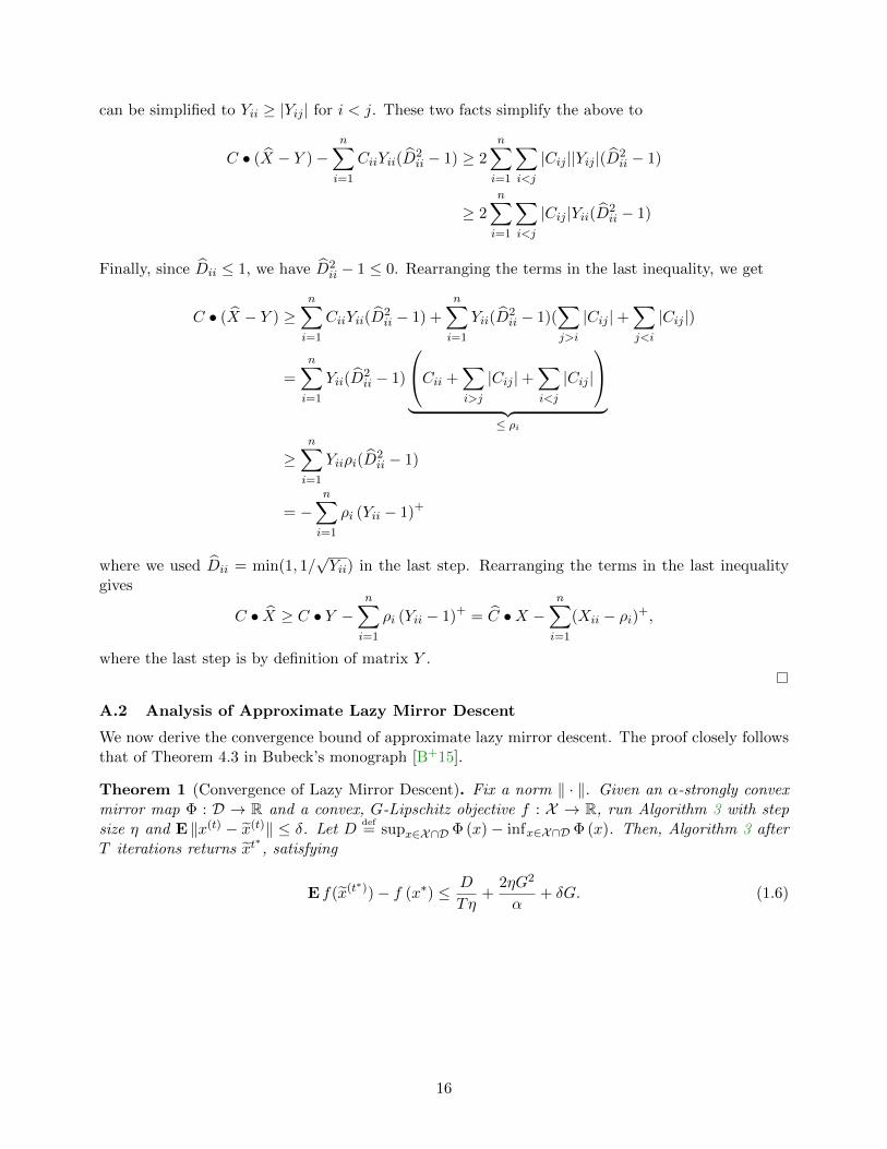
A.2 Analysis of Approximate Lazy Mirror Descent

We now derive the convergence bound of approximate lazy mirror descent. The proof closely followsthat of Theorem 4.3 in Bubeck’s monograph [B+15].

Theorem 1 (Convergence of Lazy Mirror Descent). Fix a norm ‖ · ‖. Given an α-strongly convexmirror map Φ : D → R and a convex, G-Lipschitz objective f : X → R, run Algorithm 3 with stepsize η and E ‖x(t) − x(t)‖ ≤ δ. Let D

def= supx∈X∩D Φ (x) − infx∈X∩D Φ (x). Then, Algorithm 3 after

T iterations returns xt∗, satisfying

E f(x(t∗))− f (x∗) ≤ D

Tη+

2ηG2

α+ δG. (1.6)

16

Proof. By convexity of f ,

T∑t=1

(f(x(t))− f(x)) ≤T∑t=1

⟨∇f(x(t)), x(t) − x

⟩=

T∑t=1

⟨∇f(x(t)), x(t) − x(t)

⟩︸ ︷︷ ︸

A

+

T∑t=1

⟨∇f(x(t)), x(t) − x

⟩︸ ︷︷ ︸

B

.

(A.1)

The term A can be bounded by Cauchy-Schwarz inequality and the invariant E∥∥x(t) − x(t)

∥∥ ≤ δ:A ≤

T∑t=1

∥∥∥∆(t)∥∥∥∥∥∥∇f (x(t)

)∥∥∥∗≤ δGT. (A.2)

Next, recall that Algorithm 3 initializes x(1) ∈ argminX∩D Φ(x) and z(1) satisfying ∇Φ(z(1)) = 0,and repeats the following two steps:

∇Φ(z(t)) = ∇Φ(z(t−1))− η∇f(x(t))

x(t) = argminX∩D

DΦ(x, z(t)).

Now consider the potential function Ψt(x)def= Φ(x) + η

⟨x,∑t

s=1∇f(x(s))⟩. Applying the recursive

definition of the gradient step, we can express x(t+1) = argminx∈X∩D

Ψt (x). Since Φ is α-strongly convex,

so is the potential function Ψt. We can express these two statements as follows:

Ψt(x(t+1))− Ψt(x

(t)) ≤⟨∇Ψt(x

(t+1)), x(t+1) − x(t)⟩

︸ ︷︷ ︸≤ 0, by optimality of x(t+1)

−α2

∥∥∥x(t+1) − x(t)∥∥∥2

≤ −α2

∥∥∥x(t+1) − x(t)∥∥∥2. (A.3)

We can also write a lower bound for the left hand side of Inequality A.3 by evaluating the potentialfunction Ψt at points x(t+1) and x(t):

Ψt(x(t+1))− Ψt(x

(t)) = Φ(x(t+1)

)+ η

t∑s=1

⟨∇f(x(s)), x(t+1)

⟩− Φ(x(t))− η

t∑s=1

⟨∇f(x(s)), x(t)

⟩= Ψt−1(x(t+1))− Ψt−1(x(t))︸ ︷︷ ︸≥ 0, since x(t) minimizes Ψt−1 (x)

+η⟨∇f(x(t)), x(t+1) − x(t)

⟩

≥ η⟨∇f(x(t)), x(t+1) − x(t)

⟩. (A.4)

Reverse and chain Inequalities A.3 and A.4, and apply Cauchy-Schwarz inequality to get

α

2

∥∥∥x(t+1) − x(t)∥∥∥2≤ η

⟨∇f(x(t)), x(t) − x(t+1)

⟩≤ ηG

∥∥∥x(t) − x(t+1)∥∥∥. (A.5)

This shows that ∥∥∥x(t) − x(t+1)∥∥∥ ≤ 2ηG

α, (A.6)

17

and applying this to the second part of Inequality A.5 gives⟨∇f(x(t)), x(t) − x(t+1)

⟩≤ 2ηG2

α. (A.7)

We now claim

T∑t=1

⟨∇f(x(t)), x(t) − x

⟩≤

T∑t=1

⟨∇f(x(t)), x(t) − x(t+1)

⟩+ 1

η (Φ(x)− Φ(x(1))). (A.8)

Note that this claim immediately gives the desired error bound; this can be seen as follows: theleft-hand side is exactly the term 2 in Inequality A.1; the first term of the right-hand side isbounded in Inequality A.7, and the second one is bounded by the definition of set size D. ThereforeInequality A.8 simplifies to

B ≤ 2ηG2T

α+D

η. (A.9)

Combine Inequalities A.9 and A.2 with A.1, apply Jensen’s inequality, and the fact that t∗ is pickeduniformly at random from 1, 2, . . . , T, to get the desired error bound. We now prove Inequality A.8.First, we rewrite it as

T∑t=1

⟨∇f(x(t)), x(t+1)

⟩+

Φ(x(1))

η≤

T∑t=1

⟨∇f(x(t)), x

⟩+

Φ(x)

η.

The claim is true for T = 0 for all x ∈ X , by the choice of x(1). Assume it holds for all x ∈ X attime T = t′ − 1. Therefore in particular, it holds at the point x = x(t′+1). This implies

t′∑t=1

⟨∇f(x(t)), x(t+1)

⟩+

Φ(x(1))

η=⟨∇f(x(t′)), x(t′+1)

⟩+t′−1∑t=1

⟨∇f(x(t)), x(t+1)

⟩+

Φ(x(1))

η︸ ︷︷ ︸Apply induction hypothesis at x(t′+1)

≤⟨∇f(x(t′)), x(t′+1)

⟩+t′−1∑t=1

⟨∇f(x(t)), x(t′+1)

⟩+

Φ(x(t′+1))

η

=

t′∑t=1

⟨∇f(x(t)), x(t′+1)

⟩+

Φ(x(t′+1)

)η

=1

ηΨt′

(x(t′+1)

)≤ 1

ηΨt′(x)

=

t′∑t=1

⟨∇f

(x(t)), x⟩

+Φ(x)

η,

where the last inequality is by optimality of x(t′+1) in minimizing Ψt′ . This completes the induction,and therefore proves Inequality A.8, thus completing the proof of the error bound.

18

B Analysis of the Arora-Kale Algorithm

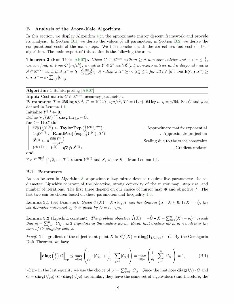
In this section, we display Algorithm 4 in the approximate mirror descent framework and provideits analysis. In Section B.1, we derive the values of all parameters; in Section B.2, we derive thecomputational costs of the main steps. We then conclude with the correctness and cost of theiralgorithm. The main export of this section is the following theorem.

Theorem 3 (Run Time [AK07]). Given C ∈ Rn×n with m ≥ n non-zero entries and 0 < ε ≤ 12 ,

we can find, in time O(m/ε5

), a matrix Y ∈ Sn with O(m) non-zero entries and a diagonal matrix

S ∈ Rn×n such that X∗ = S · K exp(Y )Tr exp(Y ) · S satisfies X∗ 0, X∗ii ≤ 1 for all i ∈ [n], and E(C • X∗) ≥

C •X∗ − ε ·∑

i,j |C|ij.

Algorithm 4 Reinterpreting [AK07]

Input: Cost matrix C ∈ Rn×n, accuracy parameter ε.Parameters: T = 256 log n/ε2, T ′ = 10240 log n/ε2, T ′′ = (1/ε) · 64 log n, η = ε/64. Set C and ρ asdefined in Lemma 1.1.Initialize Y (1) ← 0.Define ∇f(M)

def= diag 1M≥ρ − C.

for t = 1toT do

exp(

12Y

(t))← TaylorExp

(12Y

(t), T ′′). . Approximate matrix exponential

expY (t) ← RandProj(exp

(12Y

(t)), T ′). . Approximate projection

X(t) ← nexp(Y (t))Tr expY (t) . Scaling due to the trace constraint

Y (t+1) ← Y (t) − η∇f(X(t)). . Gradient update.end

For t∗unif.∼ 1, 2, . . . , T, return Y (t∗) and S, where S is from Lemma 1.1.

B.1 Parameters

As can be seen in Algorithm 3, approximate lazy mirror descent requires five parameters: the setdiameter, Lipschitz constant of the objective, strong convexity of the mirror map, step size, andnumber of iterations. The first three depend on our choice of mirror map Φ and objective f . Thelast two can be chosen based on these parameters and Inequality 1.6.

Lemma 3.1 (Set Diameter). Given Φ (X) = X • logX and the domain X : X 0,TrX = n, theset diameter measured by Φ is given by D = n log n.

Lemma 3.2 (Lipschitz constant). The problem objective f(X) = −C •X +∑n

i=1(Xii − ρi)+ (recallthat ρi =

∑nj=1 |Cij |) is 2-Lipschitz in the nuclear norm. Recall that nuclear norm of a matrix is the

sum of its singular values.

Proof. The gradient of the objective at point X is ∇f(X) = diag(1X≥ρ)− C. By the GershgorinDisk Theorem, we have

∥∥∥diag(

1ρ

)C∥∥∥

op≤ max

i∈[n]

1

ρi· |Cii|+

1

ρi·∑j 6=i|Cij |

= maxi∈[n]

1

ρi·n∑j=1

|Cij |

= 1, (B.1)

where in the last equality we use the choice of ρi =∑n

j=1 |Cij |. Since the matrices diag(1/ρ) ·C and

C = diag(1/√ρ) ·C ·diag(1/√ρ) are similar, they have the same set of eigenvalues (and therefore, the

19

same operator norm). Therefore∥∥∥diag(1X≥ρ)− C∥∥∥

op≤∥∥diag(1X≥ρ)

∥∥op

+∥∥∥C∥∥∥

op= 1 + 1 = 2.

When we have∥∥∥∇f∥∥∥ ≤ G for some G, it implies f is G-Lipschitz in ‖ · ‖∗ (the dual norm). Therefore,

in our case, we have that f is 2-Lipschitz in the nuclear norm (dual of the operator norm).

Lemma 3.3 (Strong Convexity). ([KST09]) The mirror map Φ (X) = X • logX is 1/(2n)-stronglyconvex with respect to the nuclear norm on the domain X ∈ Sn : X 0,Tr (X) = n.

Lemma 3.4. Choosing η = ε/64 and T = 256 log n/ε2 in Algorithm 4 gives an accuracy of εn.

Proof. We show in Lemma 3.10 that Algorithm 4 maintains the invariant E |||X(t) − X(t)||| ≤ δ =εn/4. Therefore we are in the framework of approximate lazy mirror descent and can use its errorbound from Inequality 1.6 and bound it by εK. We plug in the parameters from Lemmas 3.1, 3.2,and 3.3 in the bound and get

E f(x(t∗))− f(x∗) ≤ n log n

Tη+

2η · 22

1/2n+(εn

4

)· 2.

We optimize for η by setting the first two terms equal, and get

η = 14

√log n

T. (B.2)

With this expression for η, setting the bound for the right-hand side above to be εn gives T ≥256 log n/ε2; plug this back in Equation B.2 to get η = ε/64.

B.2 Computational Cost

From Algorithm 4, we see that there are three main parts to be computed to get the overall cost ofthe Arora-Kale algorithm: the number of iterations, the number of JL projections per iteration, andthe cost of approximating a matrix exponential and multiplying it with a vector. We derive thesevalues in this section.

B.2.1 Taylor Approximation for Matrix Exponential

In Algorithm 4, before we do the randomized projection to get the diagonal entries, we approxi-mate the matrix exponential exp

(Y (t)/2

)= TaylorExp

(Y (t)/2, T ′′

). Here we show a bound on∣∣∣∣ exp(Y (t))

ii

Tr exp(Y (t))− exp(Y (t))

ii

Tr exp(Y (t))

∣∣∣∣ for any 1 ≤ i ≤ n. We do so by first proving a bound on∣∣∣ Aii

TrA −BiiTrB

∣∣∣ for

a matrix B approximating the general matrix A; then we prove a general result on the number ofterms required to approximate a matrix exponential using Taylor series; finally, we combine theseresults to get an appropriate choice of Tpoly for approximating exp

(Y (t)/2

).

Lemma 3.5. Given positive definite matrices A and B such that ‖A−B‖op ≤ ε, where ε ≤ 12n TrA,

we have∣∣∣ Aii

TrA −BiiTrB

∣∣∣ ≤ 2 ε(TrA+nAii)

(TrA)2 .

Proof. We have the following chain of inequalities.∣∣∣∣ BiiTrB− Aii

TrA

∣∣∣∣ 1≤∣∣∣∣ Aii + ε

TrA− nε− Aii

TrA

∣∣∣∣ =ε (TrA+ nAii)

(TrA) (TrA− εn)

2≤ 2

ε (TrA+ nAii)

(TrA)2 ,

20

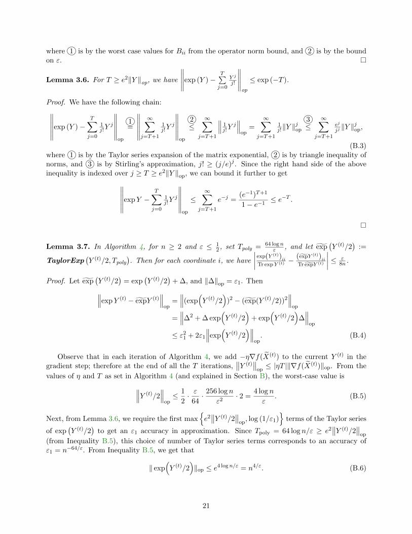
where 1 is by the worst case values for Bii from the operator norm bound, and 2 is by the boundon ε.

Lemma 3.6. For T ≥ e2‖Y ‖op, we have

∥∥∥∥∥exp (Y )−T∑j=0

Y j

j!

∥∥∥∥∥op

≤ exp (−T ).

Proof. We have the following chain:∥∥∥∥∥∥exp (Y )−T∑j=0

1j!Y

j

∥∥∥∥∥∥op

1=

∥∥∥∥∥∥∞∑

j=T+1

1j!Y

j

∥∥∥∥∥∥op

2≤

∞∑j=T+1

∥∥∥ 1j!Y

j∥∥∥

op=

∞∑j=T+1

1j!‖Y ‖

jop

3≤

∞∑j=T+1

ej

jj‖Y ‖jop,

(B.3)where 1 is by the Taylor series expansion of the matrix exponential, 2 is by triangle inequality ofnorms, and 3 is by Stirling’s approximation, j! ≥ (j/e)j . Since the right hand side of the aboveinequality is indexed over j ≥ T ≥ e2‖Y ‖op, we can bound it further to get∥∥∥∥∥∥expY −

T∑j=0

1j!Y

j

∥∥∥∥∥∥op

≤∞∑

j=T+1

e−j =(e−1)T+1

1− e−1≤ e−T .

Lemma 3.7. In Algorithm 4, for n ≥ 2 and ε ≤ 12 , set Tpoly = 64 logn

ε , and let exp(Y (t)/2

):=

TaylorExp(Y (t)/2, Tpoly

). Then for each coordinate i, we have

∣∣∣∣ exp(Y (t))ii

Tr expY (t) −(expY (t))

ii

Tr expY (t)

∣∣∣∣ ≤ ε8n .

Proof. Let exp(Y (t)/2

)= exp

(Y (t)/2

)+ ∆, and ‖∆‖op = ε1. Then∥∥∥expY (t) − expY (t)

∥∥∥op

=∥∥∥(exp

(Y (t)/2

))2 − (exp(Y (t)/2))2

∥∥∥op

=∥∥∥∆2 + ∆ exp

(Y (t)/2

)+ exp

(Y (t)/2

)∆∥∥∥

op

≤ ε21 + 2ε1

∥∥∥exp(Y (t)/2

)∥∥∥op. (B.4)

Observe that in each iteration of Algorithm 4, we add −η∇f(X(t)) to the current Y (t) in thegradient step; therefore at the end of all the T iterations,

∥∥Y (t)∥∥

op≤ |ηT |‖∇f(X(t))‖op. From the

values of η and T as set in Algorithm 4 (and explained in Section B), the worst-case value is∥∥∥Y (t)/2∥∥∥

op≤ 1

2· ε

64· 256 log n

ε2· 2 =

4 log n

ε. (B.5)

Next, from Lemma 3.6, we require the first maxe2∥∥Y (t)/2

∥∥op, log (1/ε1)

terms of the Taylor series

of exp(Y (t)/2

)to get an ε1 accuracy in approximation. Since Tpoly = 64 log n/ε ≥ e2

∥∥Y (t)/2∥∥

op

(from Inequality B.5), this choice of number of Taylor series terms corresponds to an accuracy ofε1 = n−64/ε. From Inequality B.5, we get that

‖ exp(Y (t)/2

)‖op ≤ e4 logn/ε = n4/ε. (B.6)

21

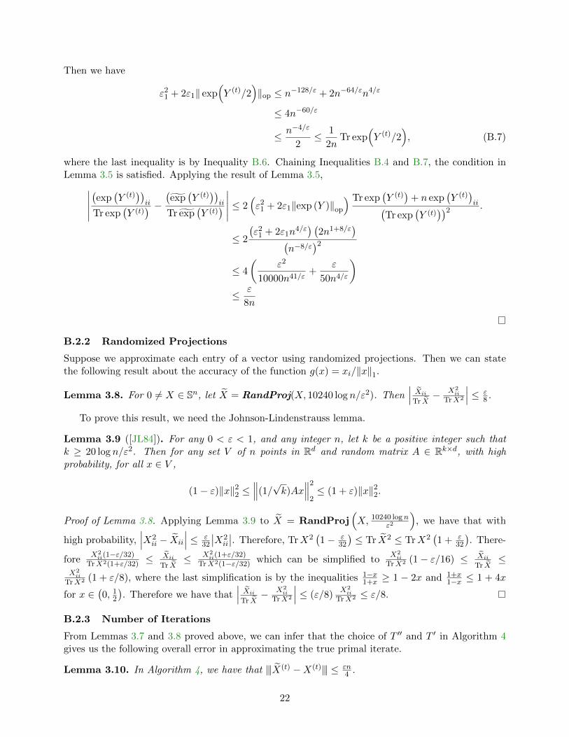
Then we have

ε21 + 2ε1‖ exp

(Y (t)/2

)‖op ≤ n−128/ε + 2n−64/εn4/ε

≤ 4n−60/ε

≤ n−4/ε

2≤ 1

2nTr exp

(Y (t)/2

), (B.7)

where the last inequality is by Inequality B.6. Chaining Inequalities B.4 and B.7, the condition inLemma 3.5 is satisfied. Applying the result of Lemma 3.5,∣∣∣∣∣

(exp

(Y (t)

))ii

Tr exp(Y (t)

) − (exp(Y (t)

))ii

Tr exp(Y (t)

) ∣∣∣∣∣ ≤ 2(ε2

1 + 2ε1‖exp (Y )‖op

) Tr exp(Y (t)

)+ n exp

(Y (t)

)ii(

Tr exp(Y (t)

))2 .

≤ 2

(ε2

1 + 2ε1n4/ε) (

2n1+8/ε)(

n−8/ε)2

≤ 4

(ε2

10000n41/ε+

ε

50n4/ε

)≤ ε

8n

B.2.2 Randomized Projections

Suppose we approximate each entry of a vector using randomized projections. Then we can statethe following result about the accuracy of the function g(x) = xi/‖x‖1.

Lemma 3.8. For 0 6= X ∈ Sn, let X = RandProj(X, 10240 log n/ε2). Then∣∣∣ Xii

Tr X− X2

iiTrX2

∣∣∣ ≤ ε8 .

To prove this result, we need the Johnson-Lindenstrauss lemma.

Lemma 3.9 ([JL84]). For any 0 < ε < 1, and any integer n, let k be a positive integer such thatk ≥ 20 log n/ε2. Then for any set V of n points in Rd and random matrix A ∈ Rk×d, with highprobability, for all x ∈ V ,

(1− ε)‖x‖22 ≤∥∥∥(1/√k)Ax

∥∥∥2

2≤ (1 + ε)‖x‖22.

Proof of Lemma 3.8. Applying Lemma 3.9 to X = RandProj(X, 10240 logn

ε2

), we have that with

high probability,∣∣∣X2

ii − Xii

∣∣∣ ≤ ε32

∣∣X2ii

∣∣. Therefore, TrX2(1− ε

32

)≤ Tr X2 ≤ TrX2

(1 + ε

32

). There-

foreX2

ii(1−ε/32)

TrX2(1+ε/32)≤ Xii

Tr X≤ X2

ii(1+ε/32)

TrX2(1−ε/32)which can be simplified to

X2ii

TrX2 (1− ε/16) ≤ Xii

Tr X≤

X2ii

TrX2 (1 + ε/8), where the last simplification is by the inequalities 1−x1+x ≥ 1 − 2x and 1+x

1−x ≤ 1 + 4x

for x ∈(0, 1

2

). Therefore we have that

∣∣∣ Xii

Tr X− X2

iiTrX2

∣∣∣ ≤ (ε/8)X2

iiTrX2 ≤ ε/8.

B.2.3 Number of Iterations

From Lemmas 3.7 and 3.8 proved above, we can infer that the choice of T ′′ and T ′ in Algorithm 4gives us the following overall error in approximating the true primal iterate.

Lemma 3.10. In Algorithm 4, we have that |||X(t) −X(t)||| ≤ εn4 .

22

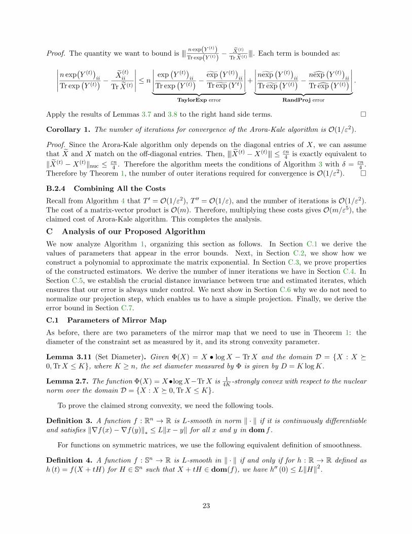
Proof. The quantity we want to bound is ||| n exp(Y (t))Tr exp(Y (t))

− X(t)

Tr X(t)|||. Each term is bounded as:

∣∣∣∣∣n exp(Y (t)

)ii

Tr exp(Y (t)

) − X(t)ii

Tr X(t)

∣∣∣∣∣ ≤ n∣∣∣∣∣ exp

(Y (t)

)ii

Tr exp(Y (t)

) − exp(Y (t)

)ii

Tr exp (Y t)

∣∣∣∣∣︸ ︷︷ ︸TaylorExp error

+

∣∣∣∣∣nexp(Y (t)

)ii

Tr exp(Y (t)

) − nexp(Y (t)

)ii

Tr exp(Y (t)

)∣∣∣∣∣︸ ︷︷ ︸RandProj error

.

Apply the results of Lemmas 3.7 and 3.8 to the right hand side terms.

Corollary 1. The number of iterations for convergence of the Arora-Kale algorithm is O(1/ε2).

Proof. Since the Arora-Kale algorithm only depends on the diagonal entries of X, we can assumethat X and X match on the off-diagonal entries. Then, |||X(t) −X(t)||| ≤ εn

4 is exactly equivalent to

‖X(t) − X(t)‖nuc ≤ εn4 . Therefore the algorithm meets the conditions of Algorithm 3 with δ = εn

4 .Therefore by Theorem 1, the number of outer iterations required for convergence is O(1/ε2).

B.2.4 Combining All the Costs

Recall from Algorithm 4 that T ′ = O(1/ε2), T ′′ = O(1/ε), and the number of iterations is O(1/ε2).The cost of a matrix-vector product is O(m). Therefore, multiplying these costs gives O(m/ε5), theclaimed cost of Arora-Kale algorithm. This completes the analysis.

C Analysis of our Proposed Algorithm

We now analyze Algorithm 1, organizing this section as follows. In Section C.1 we derive thevalues of parameters that appear in the error bounds. Next, in Section C.2, we show how weconstruct a polynomial to approximate the matrix exponential. In Section C.3, we prove propertiesof the constructed estimators. We derive the number of inner iterations we have in Section C.4. InSection C.5, we establish the crucial distance invariance between true and estimated iterates, whichensures that our error is always under control. We next show in Section C.6 why we do not need tonormalize our projection step, which enables us to have a simple projection. Finally, we derive theerror bound in Section C.7.

C.1 Parameters of Mirror Map

As before, there are two parameters of the mirror map that we need to use in Theorem 1: thediameter of the constraint set as measured by it, and its strong convexity parameter.

Lemma 3.11 (Set Diameter). Given Φ(X) = X • logX − TrX and the domain D = X : X 0,TrX ≤ K, where K ≥ n, the set diameter measured by Φ is given by D = K logK.

Lemma 2.7. The function Φ(X) = X•logX−TrX is 14K -strongly convex with respect to the nuclear

norm over the domain D = X : X 0,TrX ≤ K.

To prove the claimed strong convexity, we need the following tools.

Definition 3. A function f : Rn → R is L-smooth in norm ‖ · ‖ if it is continuously differentiableand satisfies ‖∇f(x)−∇f(y)‖∗ ≤ L‖x− y‖ for all x and y in dom f .

For functions on symmetric matrices, we use the following equivalent definition of smoothness.

Definition 4. A function f : Sn → R is L-smooth in ‖ · ‖ if and only if for h : R → R defined ash (t) = f(X + tH) for H ∈ Sn such that X + tH ∈ dom(f), we have h′′ (0) ≤ L‖H‖2.

23

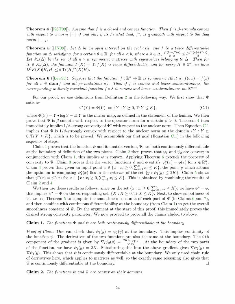
Theorem 4 ([KST09]). Assume that f is a closed and convex function. Then f is β-strongly convexwith respect to a norm ‖ · ‖ if and only if its Fenchel dual, f∗, is 1

β -smooth with respect to the dualnorm ‖ · ‖∗.

Theorem 5 ([JN08]). Let ∆ be an open interval on the real axis, and f be a twice differentiable

function on ∆ satisfying, for a certain θ ∈ R, for all a < b, where a, b ∈ ∆, f ′(b)−f ′(a)b−a ≤ θ f

′′(a)+f ′′(b)2 .

Let Xn(∆) be the set of all n × n symmetric matrices with eigenvalues belonging to ∆. Then forX ∈ Xn(∆), the function F (X) = Tr f(X) is twice differentiable, and for every H ∈ Sn, we haveD2F (X)[H,H] ≤ θTr(Hf ′′(X)H).

Theorem 6 ([Lew95]). Suppose that the function f : Rn → R is symmetric (that is, f(σx) = f(x)for all x ∈ dom f and all permutations σ). Then if f is convex and lower semicontinuous, thecorresponding unitarily invariant function f λ is convex and lower semicontinuous on Rn×n

For our proof, we use definitions from Definition 2 in the following way. We first show that Ψsatisfies

Ψ∗(Y ) = Φ(Y ), on Y : Y 0,TrY ≤ K, (C.1)

where Φ(Y ) = Y • log Y −TrY is the mirror map, as defined in the statement of the lemma. We thenprove that Ψ is β-smooth with respect to the operator norm for a certain β > 0. Theorem 4 thenimmediately implies 1/β-strong convexity of Ψ∗ with respect to the nuclear norm. Then Equation C.1implies that Φ is 1/β-strongly convex with respect to the nuclear norm on the domain Y : Y 0,TrY ≤ K, which is to be proved. We accomplish our first goal (Equation C.1) in the followingsequence of steps.

Claim 1 proves that the function ψ and its matrix version, Ψ, are both continuously differentiableat the boundary of definition of the two pieces. Claim 2 then proves that ψ1 and ψ2 are convex; inconjuncation with Claim 1, this implies ψ is convex. Applying Theorem 6 extends the property ofconvexity to Ψ. Claim 3 proves that the vector functions ψ and φ satisfy ψ∗1(x) = φ(x) for x ∈ Rn+.Claim 4 proves that given an input point x ∈ x : xi ≥ 0,

∑ni=1 xi ≤ K, the point y which attains

the optimum in computing ψ∗1(x) lies in the interior of the set y : ψ1(y) ≤ 2K. Claim 5 showsthat ψ∗(x) = ψ∗1(x) for x ∈ x : xi ≥ 0,

∑ni=1 xi ≤ K. This is obtained by combining the results of

Claim 2 and 4.We then use these results as follows: since on the set x : xi ≥ 0,

∑ni=1 xi ≤ K, we have ψ∗ = φ,

this implies Ψ∗ = Φ on the corresponding set, X : X 0,TrX ≤ K. Next, to show smoothness ofΨ, we use Theorem 5 to compute the smoothness constants of each part of Ψ (in Claims 6 and 7),and then combine with continuous differentiability at the boundary (from Claim 1) to get the overallsmoothness constant of Ψ. By the argument at the start of this proof, this immediately proves thedesired strong convexity parameter. We now proceed to prove all the claims aluded to above.

Claim 1. The functions Ψ and ψ are both continuously differentiable at the boundary.

Proof of Claim. One can check that ψ1(y) = ψ2(y) at the boundary. This implies continuity ofthe function ψ. The derivatives of the two functions are also the same at the boundary. The i-thcomponent of the gradient is given by ∇iψ2(y) = 2K∇iψ1(y)

ψ1(y) . At the boundary of the two parts

of the function, we have ψ1(y) = 2K. Substituting this into the above gradient gives ∇ψ2(y) =∇ψ1(y). This shows that ψ is continuously differentiable at the boundary. We only used chain ruleof derivatives here, which applies to matrices as well, so the exactly same reasoning also gives thatΨ is continuously differentiable at the boundary.

Claim 2. The functions ψ and Ψ are convex on their domains.

24

Proof. The function ψ is a piecewise function, each piece composed of a standard convex function(see [BV04]). Combine with continuous differentiability from Claim 1 gives convexity of ψ. ApplyingTheorem 6 implies convexity of Ψ.

Claim 3. For any input x ∈ Rn+, we have ψ∗1(x) = φ(x).

Proof of Claim. By definition, we have ψ∗1(x) = supy(x>y−

∑ni=1 exp(yi)). Observe that the domain

of ψ∗1 is Rn+ (because if there exists an input with a negative coordinate, then the correspondingcoordinate of the maximizer y∗ can be made to go to −∞). Therefore, given an input x ∈ Rn+,the supremum is attained at y∗ satisfying xi = exp(y∗i ). This means the maximizer is y∗i = log xi.Therefore the conjugate is ψ∗1(x) =

∑ni=1 xi log xi −

∑ni=1 xi = φ(x).

Claim 4. For any x in the set x : xi ≥ 0,∑n

i=1 xi ≤ K, the point y∗ = argmax(xT y − ψ1(y)

)lies

in int y : ψ1(y) ≤ 2K, where int denotes the interior of the set.

Proof of Claim. From the proof of Claim 3, for any x ∈ Rn+, we have that y∗ = argmax(xT y − ψ1(y)

)satisfies y∗i = log xi for 1 ≤ i ≤ n. In addition to this, the statement of the lemma also requiresthe input x to satisfy xi ≥ 0,

∑ni=1 xi ≤ K. Plug in the values of x in terms of y in the above

inequality to get∑n

i=1 exp y∗i ≤ K, which is the same as saying ψ1(y∗) ≤ K < 2K. This shows thatthe optimum, y∗, lies in int y : ψ1(y) ≤ 2K.

Claim 5. We have ψ∗(x) = ψ∗1(x) on all x ∈ x : xi ≥ 0,∑n

i=1 xi ≤ K.

Proof of Claim. By definition of conjugate and ψ,

ψ∗(x) = supyxT y − ψ(y) (C.2)

= supyxT y −

ψ1(y) if ψ1(y) ≤ 2Kψ2(y) otherwise

From Claim 2, ψ is convex. Therefore the function to be maximized in Equation C.2 is con-cave. From Claim 4, for input x in the set x : xi ≥ 0,

∑ni=1 xi ≤ K, we have that the maxi-

mizer argmaxy(xT y − ψ1(y)

)lies in the interior of y : ψ1(y) ≤ 2K. Therefore for input x ∈

x : xi ≥ 0,∑n

i=1 xi ≤ K, the maximizer of Equation C.2 is also the same as that of ψ∗1(x). Thisgives ψ∗(x) = ψ∗1(x).

Claim 6. The function Ψ1(Y ) defined over Y : Tr expY ≤ 2K is 4K-smooth.

Proof of Claim. Let g (u)def= exp(u). The function g is convex and differentiable (any number of

times). In particular, g′′ is convex. For any a, b, applying the Mean Value theorem to some pointζ ∈ (a, b), convexity of g′′, and g′′ ≥ 0 (due to convexity of g) gives

g′ (b)− g′ (a)

b− a= g′′ (ζ) ≤ max

(g′′ (a) , g′′ (b)

)≤ 2

g′′ (a) + g′′ (b)

2.

This satisfies the right-hand side condition for Theorem 5 with θ = 2; so Theorem 5 implies that on

25

the domain Y : Tr expY ≤ K, for h (t)def=

n∑i=1

g (λi (Y + tH)) = Tr exp(Y + tH), we have,

h′′ (0) = D2Ψ1(Y )[H,H] ≤ 2 Tr(Hg′′(Y )H

)= 2 Tr

(exp(Y )H2

)≤ 2 Tr exp(Y ) · ‖H‖2op

≤ 2 · 2K · ‖H‖2op

= 4K‖H‖2op, (C.3)

where we used the domain constraint for Ψ1 in the last inequality, and the fact that matrix exponentialis positive semidefinite in the first (Holder’s) inequality. By Definition 4 then, we have the lemma.

Claim 7. The smoothness constant of Ψ2(Y ) over the set Y : Tr expY ≥ 2K is 4K.

Proof. For ease of exposition, let adef= 2K. Consider the same scalar function from Claim 6, h (t) =

Tr exp(Y + tH) and ` (t)def= a log (h (t)) + 2K − 2K log(2K). Then `′ (t) = ah

′(t)h(t) and `′′ (t) =

a

(h′′(t)h(t) −

(h′(t)h(t)

)2)≤ ah

′′(t)h(t) . In particular,

`′′ (0) ≤ ah′′(0)

h(0). (C.4)

We already showed in Inequality C.3 that h′′ (0) = D2Ψ1(Y )[H,H] ≤ 4K‖H‖2op. We also have thath(0) = Tr exp(Y ) ≥ 2K (by assumption of the lemma). Plugging these along with the value of a intoInequality C.4 gives us `′′ (0) ≤ 2K 4K

2K · ‖H‖2op = 4K‖H‖2op. This implies the claimed smoothness

constant.

Proof of Lemma 2.7. For the functions defined in Definition 2, we can combine Claims 3 and 5 toget that ψ∗(x) = φ(x) for x ∈ x : xi ≥ 0,

∑ni=1 xi ≤ K. This implies the matrix version of this

statement, Ψ∗(X) = Φ(X) for X ∈ X : X 0,TrX ≤ K. Next, applying Claims 1, 6, and 7,we get that the function Ψ is continuously differentiable with smoothness constant 4K. InvokingTheorem 4, we immediately obtain that Ψ∗ is strongly convex with parameter 1

4K . This implies thatΦ is strongly convex with the same parameter over the set X : X 0,TrX ≤ K.

C.2 Chebyshev Approximation of the Matrix Exponential

In this section, we show how to construct a polynomial approximation of our matrix exponential.The standard technique to do so involves truncating the Taylor series of the matrix exponential;however, a quadratically improved bound on the number of terms required for the computation isprovided by Sachdeva and Vishnoi [SV+14] using Chebyshev polynomials. We follow their notationand summarize their main results below for the sake of completeness.

C.2.1 A Brief Summary of Chebyshev Approximation

For a non-negative integer d, we denote by Td(x) the Chebyshev polynomials of degree d, definedrecursively as follows:

T0(x) = 1,

T1(x) = x,

Td(x) = 2xTd−1(x)− Td−2(x).

26

Let Yi be i.i.d. variables taking values 1 and −1 each with probability 1/2. Let Ds =∑s

i=1 Yi,

D0def= 0, and

ps,d(x)def= EY1,Y2,...,Ys

(TDs(x)1|Ds|≤d

). (C.5)

We can use these to construct a polynomial with degree roughly√s that can well approximate xs.

The formal statement follows.

Theorem 7 (Theorem 3.3 in [SV+14]). For any positive integers s and d, the degree d polynomialps,d defined by Equation C.5 satisfies

supx∈[−1,1]

|ps,d(x)− xs| ≤ 2 exp(−d2/(2s)

).

Using this result, define the polynomial:

qλ,t,d(x)def= exp(−λ)

t∑i=0

(−λ)i

i!pi,d(x). (C.6)

Then we can use q to approximate an exponential with the following error guarantee.

Lemma 7.1 (Lemma 4.2 of [SV+14]). For every λ > 0 and δ ∈ (0, 1/2], we can choose t =max(λ, log(1/δ)) and d =

√t log(1/δ) such that

supx∈[−1,1]

|exp(−λ− λx)− qλ,t,d(x)| ≤ δ.

This is a quadratic improvement over the standard cost (degree) of approximating an exponentialusing truncated Taylor series. Finally, this lemma can be used to generalize the approximation fromthe [−1, 1] interval to the interval [0, b], as stated below.

Theorem 8 (Theorem 4.1 of [SV+14]). For every b > 0, and 0 < δ ≤ 1, there exists a polynomialrb,δ that satisfies

supx∈[0,b]

|exp(−x)− rb,δ(x)| ≤ δ

and has degree O(√

max(b, log(1/δ)) · log(1/δ)).

The proof of this theorem uses λdef= b/2, and t and d from Lemma 7.1 and the polynomial

rb,δ(x)def= qλ,t,d

(1

λ(x− λ)

). (C.7)

Corollary 2 (Our Chebyshev Approximation). For every b > 0, a < b, 0 < δ ≤ 1, and d =√max

(12(b− a), log

(1δ

))log(

1δ

), there exists a degree-d polynomial ChebyExp(u, d, δ) such that

supu∈[a,b]

|exp(u)−ChebyExp(u, d, δ)| ≤ δ exp(b). (C.8)

Proof. Using a simple linear transformation, Theorem 8 generalizes to:

supz∈[a,b]

∣∣∣∣∣exp

(−1

2(b− a)

) t∑i=0

(−12(b− a))i

i!pi,d(

z − (b+ a)/2

(b− a)/2)− exp(−(z − a))

∣∣∣∣∣ ≤ δ.27

By choosing λ = 12(b− a), and transforming −z + a = u− b, we get

supu∈[a,b]

∣∣∣∣q12 (b−a),t,d

(−u+ (b+ a)/2

(b− a)/2

)− exp(u− b)

∣∣∣∣ ≤ δ.Using Equation C.7 above gives

supu∈[a,b]

|exp(b)rb−a,δ(b− u)− exp(u)| ≤ δ exp(b).

Therefore, let d =√

max(

12(b− a), log

(1δ

))log(

1δ

)and ChebyExp(u, d, δ) = exp(b)rb−a,δ(b − u).

Substitute these into the last inequality to get the statement of the lemma.

C.2.2 Chebyshev Approximation in Our Algorithm

We can use the above results to approximate a matrix exponential as follows. Observe that

‖exp(Y )−ChebyExp(Y, d, δ)‖op = maxi∈[n]|exp(λi)−ChebyExp(λi, d, δ)|,

where λi are the eigenvalues of Y and ChebyExp is the subroutine described in Corollary 2. Weonly need the spectrum of Y in order to complete the approximation, and that is what we proceedto derive below. Once we have the spectrum, we simply combine it with the above results to getLemma 8.2.

Lemma 8.1. The spectrum of Y lies in the range[−1ε60 log n, logK

].

Proof. Since we start Algorithm 1 with Y (1) = 0, at the t-th iteration, we have Y (t) = −∑t−1

i=1 η∇f(X(i)

).

Plugging in the parameters displayed in Table 1, we get that the total number of iterations of thealgorithm is Tinner × Touter = 1

ε324 × 105 (log(n/ε))11 log n, the Lipschitz constant of the objective

function is ‖∇f‖op ≤ 2, and the step size is η = ε2

8×104(log(n/ε))11 . Multiplying these gives

∥∥∥Y (t)∥∥∥

op≤ 2 · ε2

8× 104 × (log(n/ε))11 ·24× 105 × (log(n/ε))11 log n

ε3=

1

ε60 log n.

Therefore, the spectrum of Y (t) lies in

λ(Y (t)) ∈[−1

ε60 log n,

1

ε60 log n

]. (C.9)

We now show a better upper bound on the spectrum. Since our algorithm maintains TrX(t) ≤ K(see Lemma 2.6), and X(t) = exp

(Y (t)

), it implies Tr exp

(Y (t)

)≤ K. Since the matrix exponential

is positive definite, this implies∥∥exp

(Y (t)

)∥∥op≤ K, and therefore,

λmax(Y (t)) ≤ logK. (C.10)

Combining the inclusion C.9 and Inequality C.10 gives the claimed bound on the spectrum.

Lemma 8.2. In Algorithm 4, for n ≥ 2 and ε ≤ 12 , set TCheby = 150√

εlog(n/ε), δCheby = (ε/n)401,

and let exp(Y (t)/2

):= ChebyExp

(Y (t)/2,TCheby, δCheby

). Then for all 1 ≤ i ≤ n,∣∣∣exp

(Y (t)

)ii−(

expY (t))ii

∣∣∣ ≤ δexpdef= 4800ε401

n390 .

28

Proof. We plug into Inequality C.8 the following bounds obtained from Lemma 8.1:

a = −60 lognε , b = logK

u = λ = 12(b− a) = logK

2 + 30 lognε

Applying Inequality C.8, we then get

sup

λ∈[−30 logn

ε ,12 logK

]∣∣∣∣Kr1

2 logK+30 logn

ε ,δ

(12 logK − 1

2λ)− exp

(12λ)∣∣∣∣ ≤ δK

We have K = 40n (log n)10; therefore, if we want the error bound to be roughly εn , then we need to

pick δ = polylog(ε, n). Because of technical details in Lemma 9.1, we choose

δCheby =( εn

)401. (C.11)

This gives us the following result.∥∥∥exp(Y (t)/2

)−ChebyExp(Y (t)/2,TCheby, δCheby)

∥∥∥op≤ 40

ε401

n396.

From Lemma 7.1, we get that the degree of polynomial required to achieve this guarantee is

Required Degree =

√2× 104

εlog n log(n/ε) ≤ 150√

εlog(n/ε).

This is the value of TCheby that we choose. We now bound the quantity we actually care about. We

can write exp(

12Y

(t))

= exp(

12Y

(t))

+∆, where ‖∆‖op = 40 ε401

n396 , the error guarantee obtained above.

Simplifying with the application of∥∥exp

(Y (t)

)∥∥op≤ K obtained from Lemma 2.6 gives

∥∥∥exp(Y (t)

)− exp

(Y (t)

)∥∥∥op

=

∥∥∥∥(exp(

12Y

(t)))2−(

exp(

12Y

(t)))2

∥∥∥∥op

=∥∥∥∆2 + ∆ exp

(12Y

(t))

+ exp(

12Y

(t))

∆∥∥∥

op

≤ (40ε401

n396)2 + 2(40

ε401

n396)∥∥∥exp

(12Y

(t))∥∥∥

op

≤ (40ε401

n396)2 + 2(40

ε401

n396)K

≤ 3(40ε401

n396)K

≤ 3 · 40ε401

n396· 40n (log n)10

≤ 4800ε401

n390.

Substituting our assumption n ≥ 4 above gives the claimed bound.

In conclusion, we showed that we can approximate our matrix exponential to ε-accuracy usingO(1/

√ε) terms in the polynomial approximation.

29

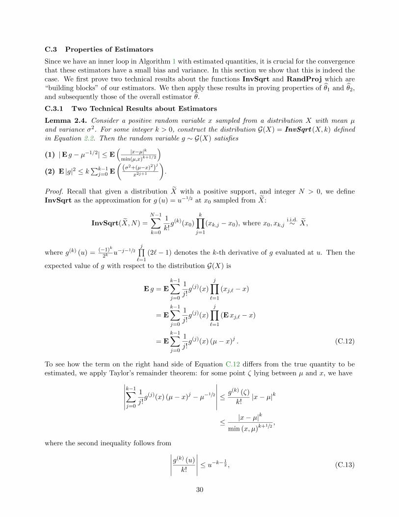
C.3 Properties of Estimators

Since we have an inner loop in Algorithm 1 with estimated quantities, it is crucial for the convergencethat these estimators have a small bias and variance. In this section we show that this is indeed thecase. We first prove two technical results about the functions InvSqrt and RandProj which are“building blocks” of our estimators. We then apply these results in proving properties of θ1 and θ2,and subsequently those of the overall estimator θ.

C.3.1 Two Technical Results about Estimators

Lemma 2.4. Consider a positive random variable x sampled from a distribution X with mean µand variance σ2. For some integer k > 0, construct the distribution G(X) = InvSqrt (X, k) definedin Equation 2.2. Then the random variable g ∼ G(X) satisfies

(1) |E g − µ−1/2| ≤ E(

|x−µ|k

min(µ,x)k+1/2

)(2) E |g|2 ≤ k

∑k−1j=0 E

((σ2+(µ−x)2)

j

x2j+1

).

Proof. Recall that given a distribution X with a positive support, and integer N > 0, we defineInvSqrt as the approximation for g (u) = u−1/2 at x0 sampled from X:

InvSqrt(X,N) =

N−1∑k=0

1

k!g(k)(x0)

k∏j=1

(xk,j − x0), where x0, xk,ji.i.d.∼ X,

where g(k) (u) = (−1)k

2ku−j−1/2

j∏`=1

(2`− 1) denotes the k-th derivative of g evaluated at u. Then the

expected value of g with respect to the distribution G(X) is

E g = E

k−1∑j=0

1

j!g(j)(x)

j∏`=1

(xj,` − x)

= E

k−1∑j=0

1

j!g(j)(x)

j∏`=1

(Exj,` − x)

= E

k−1∑j=0

1

j!g(j)(x) (µ− x)j . (C.12)

To see how the term on the right hand side of Equation C.12 differs from the true quantity to beestimated, we apply Taylor’s remainder theorem: for some point ζ lying between µ and x, we have∣∣∣∣∣∣

k−1∑j=0

1

j!g(j)(x) (µ− x)j − µ−1/2

∣∣∣∣∣∣ ≤ g(k) (ζ)

k!|x− µ|k

≤ |x− µ|k

min (x, µ)k+1/2,

where the second inequality follows from∣∣∣∣∣g(k) (u)

k!

∣∣∣∣∣ ≤ u−k− 12 , (C.13)

30

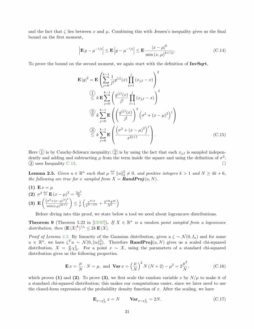
and the fact that ζ lies between x and µ. Combining this with Jensen’s inequality gives us the finalbound on the first moment,∣∣∣E g − µ−1/2

∣∣∣ ≤ E∣∣∣g − µ−1/2

∣∣∣ ≤ E|x− µ|k

min (x, µ)k+1/2. (C.14)

To prove the bound on the second moment, we again start with the definition of InvSqrt,

E |g|2 = E

k−1∑j=0

1

j!g(j)(x)

j∏`=1

(xj,` − x)

2

1≤ kE

k−1∑j=0

(g(j)(x)

j!

j∏`=1

(xj,` − x)

)2

2= k

k−1∑j=0

E

(g(j)(x)

j!

)2 (σ2 + (x− µ)2

)j3≤ k

k−1∑j=0

E

(σ2 + (x− µ)2

)jx2j+1

. (C.15)

Here 1 is by Cauchy-Schwarz inequality; 2 is by using the fact that each xj,` is sampled indepen-dently and adding and subtracting µ from the term inside the square and using the definition of σ2;3 uses Inequality C.13.

Lemma 2.5. Given u ∈ Rn such that µdef= ‖u‖22 6= 0, and positive integers k > 1 and N ≥ 4k + 6,

the following are true for x sampled from X = RandProj (u,N).

(1) Ex = µ

(2) σ2 def= E (x− µ)2 = 2µ2

N

(3) E

((σ2+(x−µ)2)

k

min(x,µ)2k+1

)≤ 1

µ

(eN/2

2N−17k + 213kk2k

Nk

)Before diving into this proof, we state below a tool we need about logconcave distributions.

Theorem 9 (Theorem 5.22 in [LV07]). If X ∈ Rn is a random point sampled from a logconcavedistribution, then (E |X|k)1/k ≤ 2kE |X|.

Proof of Lemma 2.5. By linearity of the Gaussian distribution, given a ζ ∼ N (0, In) and for someu ∈ Rn, we have ζTu ∼ N (0, ‖u‖22). Therefore RandProj(u,N) gives us a scaled chi-squareddistribution, X = µ

Nχ2N . For a point x ∼ X, using the parameters of a standard chi-squared

distribution gives us the following properties.

Ex =µ

N·N = µ, and Varx =

( µN

)2N (N + 2)− µ2 = 2

µ2

N, (C.16)

which proves (1) and (2). To prove (3), we first scale the random variable x by N/µ to make it ofa standard chi-squared distribution; this makes our computations easier, since we later need to usethe closed-form expression of the probability density function of x. After the scaling, we have

Ex∼χ2Nx = N Varx∼χ2

N= 2N. (C.17)

31

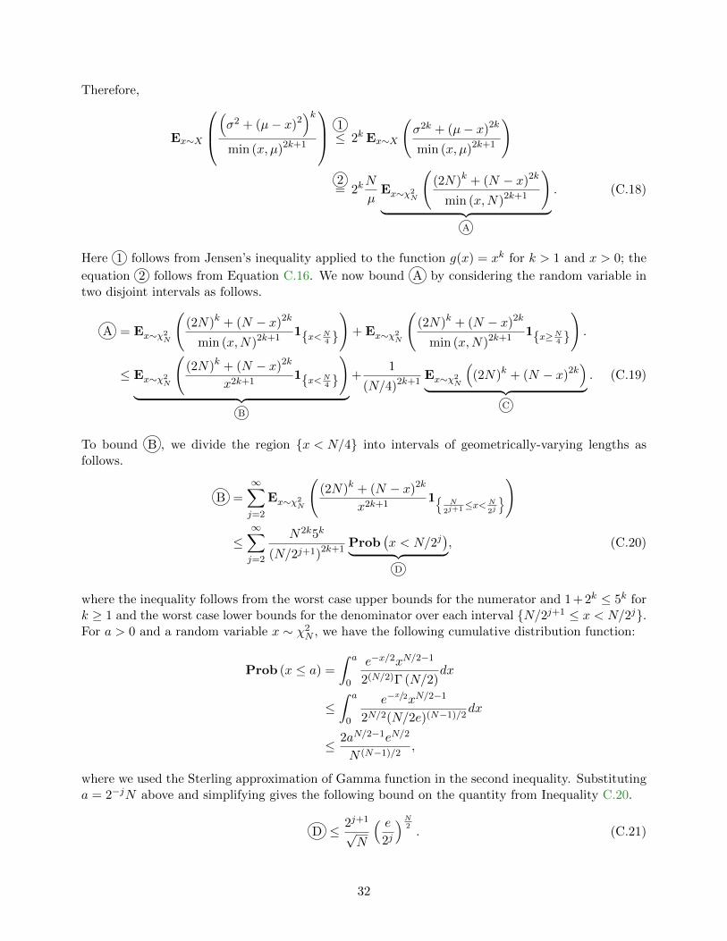
Therefore,

Ex∼X

(σ2 + (µ− x)2

)kmin (x, µ)2k+1

1≤ 2k Ex∼X

(σ2k + (µ− x)2k

min (x, µ)2k+1

)

2= 2k

N

µEx∼χ2

N

((2N)k + (N − x)2k

min (x,N)2k+1

)︸ ︷︷ ︸

A

. (C.18)

Here 1 follows from Jensen’s inequality applied to the function g(x) = xk for k > 1 and x > 0; the

equation 2 follows from Equation C.16. We now bound A by considering the random variable intwo disjoint intervals as follows.

A = Ex∼χ2N

((2N)k + (N − x)2k

min (x,N)2k+11x<N

4

)+ Ex∼χ2

N

((2N)k + (N − x)2k

min (x,N)2k+11x≥N

4

).

≤ Ex∼χ2N

((2N)k + (N − x)2k

x2k+11x<N

4

)︸ ︷︷ ︸

B

+1

(N/4)2k+1Ex∼χ2

N

((2N)k + (N − x)2k

)︸ ︷︷ ︸

C

. (C.19)

To bound B , we divide the region x < N/4 into intervals of geometrically-varying lengths asfollows.

B =∞∑j=2

Ex∼χ2N

((2N)k + (N − x)2k

x2k+11 N

2j+1≤x<N

2j

)

≤∞∑j=2

N2k5k

(N/2j+1)2k+1Prob

(x < N/2j

)︸ ︷︷ ︸D

, (C.20)

where the inequality follows from the worst case upper bounds for the numerator and 1+2k ≤ 5k fork ≥ 1 and the worst case lower bounds for the denominator over each interval N/2j+1 ≤ x < N/2j.For a > 0 and a random variable x ∼ χ2

N , we have the following cumulative distribution function:

Prob (x ≤ a) =

∫ a

0

e−x/2xN/2−1

2(N/2)Γ (N/2)dx

≤∫ a

0

e−x/2xN/2−1

2N/2(N/2e)(N−1)/2dx

≤ 2aN/2−1eN/2

N (N−1)/2,

where we used the Sterling approximation of Gamma function in the second inequality. Substitutinga = 2−jN above and simplifying gives the following bound on the quantity from Inequality C.20.

D ≤ 2j+1

√N

( e2j

)N2. (C.21)

32

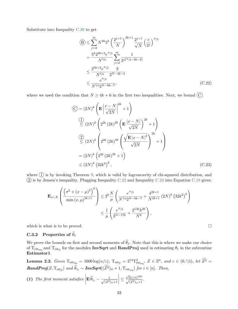
Substitute into Inequality C.20 to get

B ≤∞∑j=2

N2k5k(

2j+1

N

)2k+12j+1

√N

( e2j

)N/2

=5k22k+2eN/2

N 3/2

∞∑j=2

1

2j(N/2−2k−2)

≤ 25k+2eN/2

N 3/2

2

2N−4k−4

≤ eN/2

N 3/22N−9k−7, (C.22)

where we used the condition that N ≥ 4k + 6 in the first two inequalities. Next, we bound C .

C = (2N)k(

E

∣∣∣∣x−N√2N

∣∣∣∣2k + 1

)1≤ (2N)k

(22k (2k)2k

(E|x−N |√

2N

)2k

+ 1

)

2≤ (2N)k

22k (2k)2k

√

E |x−N |2√

2N

2k

+ 1

= (2N)k

(22k (2k)2k + 1

)≤ (2N)k

(32k2

)k, (C.23)

where 1 is by invoking Theorem 9, which is valid by logconcavity of chi-squared distribution, and2 is by Jensen’s inequality. Plugging Inequality C.22 and Inequality C.23 into Equation C.18 gives:

Ex∼X

(σ2 + (x− µ)2

)kmin (x, µ)2k+1

≤ 2kN

µ

(eN/2

N 3/22N−9k−7+

42k+1

N2k+1(2N)k

(32k2

)k)

≤ 1

µ

(eN/2

2N−17k+

213kk2k

Nk

),

which is what is to be proved.

C.3.2 Properties of θ1

We prove the bounds on first and second moments of θ1. Note that this is where we make our choiceof Testisq and Testjl

for the modules InvSqrt and RandProj used in estimating θ1 in the subroutineEstimator1.

Lemma 2.2. Given Testisq = 1600 log(n/ε), Testjl= 214T2

estisq, Z ∈ Sn, and ε ∈ (0, 1/2), let Z2 =

RandProj(Z,Testjl) and θ1i ∼ InvSqrt((Z2)ii + 1,Testisq) for i ∈ [n]. Then,

(1) The first moment satisfies

∣∣∣∣E θ1i − 1√(Z2)ii+1

∣∣∣∣ ≤ √2(ε/n)400√(Z2)ii+1

.

33

(2) The second moment satisfies E |θ1i |2 ≤ 1(Z2)ii

1630 log(n/ε).

Proof. Consider a random variable x sampled from the distribution (Z2)ii. Because of Lemma 2.5,we have Ex = (Z2)ii. Then x+ 1 satisfies the required bias condition of Lemma 2.4 for constructinga polynomial approximation for 1/

√1 + (Z2)ii. Then θ1i satisfies∣∣∣∣∣E θ1i −

1√1 + (Z2)ii

∣∣∣∣∣ 1≤ E

( ∣∣x− (Z2)ii∣∣Testisq

min(x+ 1, (Z2)ii + 1)Testisq+1/2

)2≤

√E

(x− (Z2)ii)2Testisq

min (x+ 1, (Z2)ii + 1)2Testisq+1

3≤

√√√√ 1

(Z2)ii + 1

(eTestjl/2

2Testjl−17Testisq

+213Testisq Testisq

2Testisq

Testjl

Testisq

).

where 1 is by Lemma 2.4, 2 is by Jensen’s inequality, and 3 is by a slight modification of theproof of (3) in Lemma 2.5 (instead of scaling by N/µ, we scale by Nµ/(µ+ 1) in the proof). Finally,set Testisq = 1600 log

(nε

)and Testjl

= 214T2estisq

to get the claimed bias. Next, we can bound thevariance as follows.

E |θ1i |21≤ Testisq

Testisq−1∑k=0

E

(σ2 +

(x− (Z2)ii

)2)k(x+ 1)2k+1

≤ Testisq

Testisq−1∑k=0

E

(σ2 +

(x− (Z2)ii

)2)kmin (x+ 1, (Z2)ii + 1)2k+1

2≤

Testisq

(Z2)ii

Testisq−1∑k=0

(eTestjl

/2

2Testjl−17k

+213kk2k

Tkestjl

)

3=

Testisq

(Z2)ii

Testisq−1∑k=0

(217k

(√e

2

)214T2estisq

+k2k

2kT2kestisq

)

where 1 is by (2) in Lemma 2.4, 2 is by (3) in Lemma 2.5, and 3 is by writing Testjlin terms of

Testisq . We have the simplications,∑Testisq−1

k=0 217k(√

e2

)214T2estisq ≤ 2

17Testisq

1.2214Testisq 216

and

Testisq−1∑k=0

(k2

2T2estisq

)k≤ 1 +

1

2T2estisq

+4

T4estisq

+

Testisq/2∑k=3

(k2

2T2estisq

)k+

∑k>Testisq/2

(k2

2T2estisq

)k.

Finally, plug in the values of Testisq to get the desired bound.

In Algorithm 1, we construct the matrix Z as an approximation to exp(

12

(Y (t) + s∆

))by the

subroutine ChebyExp(

12

(Y (t) + s∆

), TCheby, δCheby

), with details as provided in Lemma 8.2. With

this value of Z and the same rest of the notation as in the above lemma, we therefore wish tocompare E θ1i with 1√

exp(Y (t−1)+s∆)ii

+1. Note that the above lemma only tells us that we are close to

34

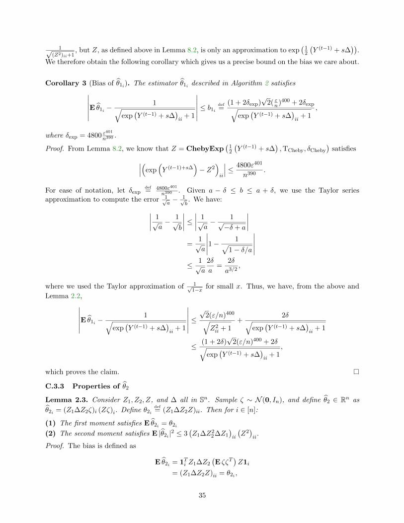
1√(Z2)ii+1

, but Z, as defined above in Lemma 8.2, is only an approximation to exp(

12

(Y (t−1) + s∆

)).

We therefore obtain the following corollary which gives us a precise bound on the bias we care about.

Corollary 3 (Bias of θ1i). The estimator θ1i described in Algorithm 2 satisfies∣∣∣∣∣∣E θ1i −1√

exp(Y (t−1) + s∆

)ii

+ 1

∣∣∣∣∣∣ ≤ b1i def=

(1 + 2δexp)√

2( εn)400 + 2δexp√exp

(Y (t−1) + s∆

)ii

+ 1,

where δexp = 4800 ε401

n390 .

Proof. From Lemma 8.2, we know that Z = ChebyExp(

12

(Y (t−1) + s∆

),TCheby, δCheby

)satisfies∣∣∣(exp

(Y (t−1)+s∆

)− Z2

)ii

∣∣∣ ≤ 4800ε401

n390.

For ease of notation, let δexpdef= 4800ε401

n390 . Given a − δ ≤ b ≤ a + δ, we use the Taylor seriesapproximation to compute the error 1√

a− 1√

b. We have:∣∣∣∣ 1√

a− 1√

b

∣∣∣∣ ≤ ∣∣∣∣ 1√a− 1√−δ + a

∣∣∣∣=

1√a

∣∣∣∣∣1− 1√1− δ/a

∣∣∣∣∣≤ 1√

a

2δ

a=

2δ

a3/2,

where we used the Taylor approximation of 1√1−x for small x. Thus, we have, from the above and

Lemma 2.2,∣∣∣∣∣∣E θ1i −1√

exp(Y (t−1) + s∆

)ii

+ 1

∣∣∣∣∣∣ ≤√

2(ε/n)400√Z2ii + 1

+2δ√

exp(Y (t−1) + s∆

)ii

+ 1

≤ (1 + 2δ)√

2(ε/n)400 + 2δ√exp

(Y (t−1) + s∆

)ii

+ 1,

which proves the claim.

C.3.3 Properties of θ2

Lemma 2.3. Consider Z1, Z2, Z, and ∆ all in Sn. Sample ζ ∼ N (0, In), and define θ2 ∈ Rn as

θ2i = (Z1∆Z2ζ)i (Zζ)i. Define θ2idef= (Z1∆Z2Z)ii. Then for i ∈ [n]:

(1) The first moment satisfies E θ2i = θ2i

(2) The second moment satisfies E |θ2i |2 ≤ 3(Z1∆Z2

2∆Z1

)ii

(Z2)ii

.

Proof. The bias is defined as

E θ2i = 1Ti Z1∆Z2

(E ζζT

)Z1i

= (Z1∆Z2Z)ii = θ2i ,

35

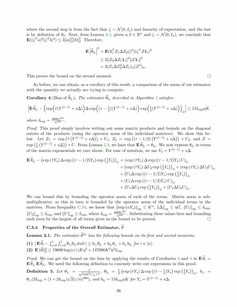
where the second step is from the fact that ζ ∼ N (0, In) and linearity of expectation, and the lastis by definition of θ2. Next, from Lemma 9.1, given a, b ∈ Rn and ζ ∼ N (0, In), we conclude thatE((ζTa)2(ζT b)2) ≤ 3‖a‖22‖b‖

22. Therefore,

E∣∣∣θ2i

∣∣∣2 = E(1Ti Z1∆Z2ζ)2)(ζTZ1i)2

≤ 3‖Z2∆Z11i‖2‖Z1i‖2

= 3(Z1∆Z22∆Z1)ii(Z

2)ii.

This proves the bound on the second moment.

As before, we can obtain, as a corollary of this result, a comparison of the mean of our estimatorwith the quantity we actually are trying to compute.

Corollary 4 (Bias of θ2i). The estimator θ2i described in Algorithm 2 satisfies∣∣∣E θ2i −(

exp(τ(Y (t−1) + s∆)

)∆ exp

((τ − 1

2)(Y (t−1) + s∆))

exp(

12(Y (t−1) + s∆)

))ii

∣∣∣ ≤ 15δexpηK

where δexp = 4800ε401

n390 .

Proof. This proof simply involves writing out some matrix products and bounds on the diagonalentries of the products (using the operator norm of the individual matrices). We show this be-low. Let Z1 = exp

(τ(Y (t−1) + s∆

))+ U1, Z2 = exp

((τ − 1/2)

(Y (t−1) + s∆

))+ U2, and Z =

exp(

12

(Y (t−1) + s∆

))+U . From Lemma 2.3, we have that E θ2i = θ2i . We now express θ2i in terms

of the matrix exponentials we care about. For ease of notation, we use Ys = Y (t−1) + s∆.

E θ2i −(exp (τYs) ∆ exp ((τ − 1/2)Ys) exp

(12Ys))ii

= (exp (τYs) ∆ exp ((τ − 1/2)Ys)U)ii

+(exp (τYs) ∆U2 exp

(12Ys))ii

+ (exp (τYs) ∆U2U)ii

+(U1∆ exp ((τ − 1/2)Ys) exp

(12Ys))ii

+ (U1∆ exp ((τ − 1/2)Ys)U)ii+(U1∆U2 exp

(12Ys))ii

+ (U1∆U2U)ii .

We can bound this by bounding the operator norm of each of the terms. Matrix norm is sub-multiplicative, so this in turn is bounded by the operator norm of the individual terms in thematrices. From Inequality C.10, we know that ‖exp (αYs)‖op ≤ Kα, ‖∆‖op ≤ ηG, ‖U1‖op ≤ δexp,

‖U2‖op ≤ δexp, and ‖U‖op ≤ δexp, where δexp = 4800ε401

n390 . Substituting these values here and boundingeach term by the largest of all terms gives us the bound to be proved.

C.3.4 Properties of the Overall Estimator, θ

Lemma 2.1. The estimator θ(t) has the following bounds on its first and second moments.

(1) |E θi −∫ 1s=0

∫ 1τ=0 θ1iθ2idsdτ | ≤ b1iθ2i + b2iθ1i + b1ib2i for i ∈ [n].

(2) E ‖θ‖22 ≤ 19600 log(n/ε)Kη2 + 147000K2η2δexp.

Proof. We can get the bound on the bias by applying the results of Corollaries 3 and 4 in E θi =E θ1i E θ2i . We need the following definition to concisely write out expressions in this proof.

Definition 5. Let θ1i = 1√exp(Ys)ii+1

, θ2i = 12

(exp (τYs) ∆ exp

((τ − 1

2)Ys)

exp(

12Ys))ii

, b1i =

θ1i(2δexp + (1 + 2δexp)√

2(ε/n)400), and b2i = 15δexpηK for Ys = Y (t−1) + s∆.

36

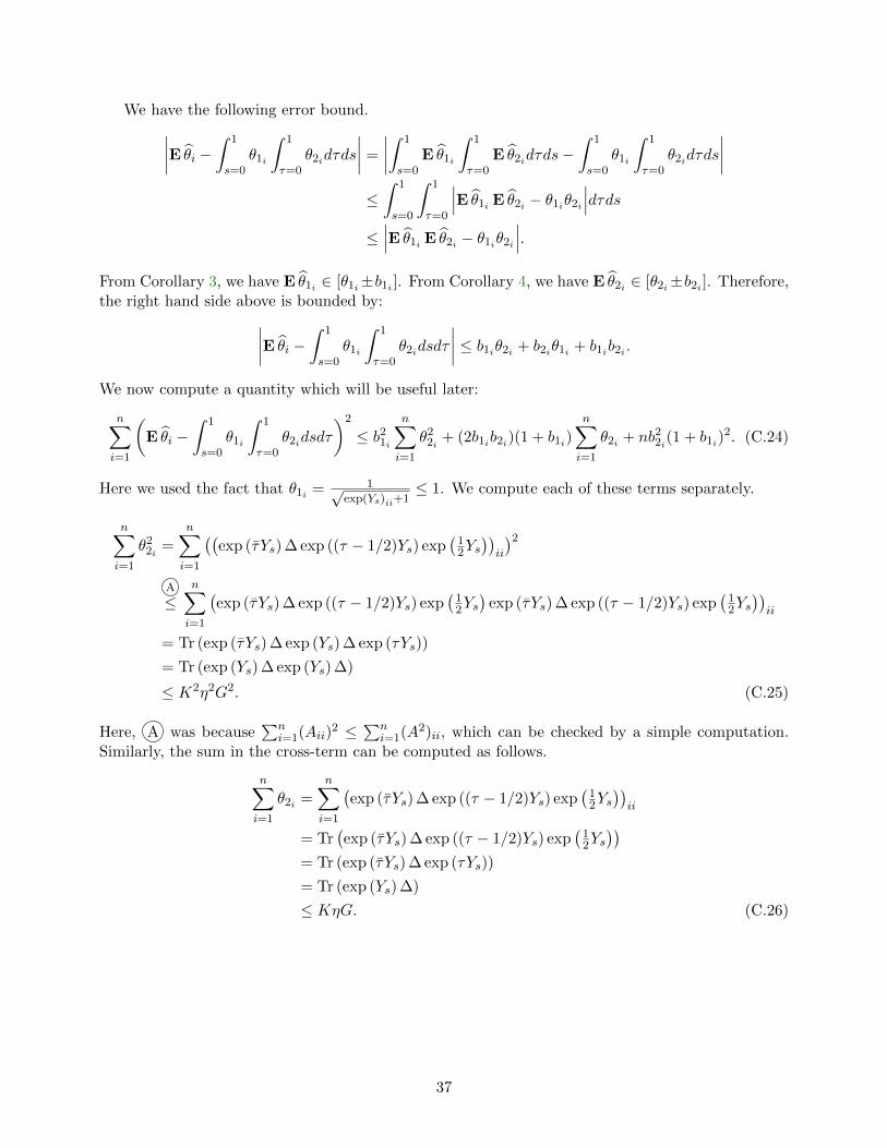
We have the following error bound.∣∣∣∣E θi −∫ 1

s=0θ1i

∫ 1

τ=0θ2idτds

∣∣∣∣ =

∣∣∣∣∫ 1

s=0E θ1i

∫ 1

τ=0E θ2idτds−

∫ 1

s=0θ1i

∫ 1

τ=0θ2idτds

∣∣∣∣≤∫ 1

s=0

∫ 1

τ=0

∣∣∣E θ1i E θ2i − θ1iθ2i

∣∣∣dτds≤∣∣∣E θ1i E θ2i − θ1iθ2i

∣∣∣.From Corollary 3, we have E θ1i ∈ [θ1i±b1i ]. From Corollary 4, we have E θ2i ∈ [θ2i±b2i ]. Therefore,the right hand side above is bounded by:∣∣∣∣E θi −

∫ 1

s=0θ1i

∫ 1

τ=0θ2idsdτ

∣∣∣∣ ≤ b1iθ2i + b2iθ1i + b1ib2i .

We now compute a quantity which will be useful later:

n∑i=1

(E θi −

∫ 1

s=0θ1i

∫ 1

τ=0θ2idsdτ

)2

≤ b21in∑i=1

θ22i + (2b1ib2i)(1 + b1i)

n∑i=1

θ2i + nb22i(1 + b1i)2. (C.24)

Here we used the fact that θ1i = 1√exp(Ys)ii+1

≤ 1. We compute each of these terms separately.

n∑i=1

θ22i =

n∑i=1

((exp (τYs) ∆ exp ((τ − 1/2)Ys) exp

(12Ys))ii

)2A

≤n∑i=1

(exp (τYs) ∆ exp ((τ − 1/2)Ys) exp

(12Ys)

exp (τYs) ∆ exp ((τ − 1/2)Ys) exp(

12Ys))ii

= Tr (exp (τYs) ∆ exp (Ys) ∆ exp (τYs))

= Tr (exp (Ys) ∆ exp (Ys) ∆)

≤ K2η2G2. (C.25)

Here, A was because∑n

i=1(Aii)2 ≤

∑ni=1(A2)ii, which can be checked by a simple computation.

Similarly, the sum in the cross-term can be computed as follows.

n∑i=1

θ2i =

n∑i=1

(exp (τYs) ∆ exp ((τ − 1/2)Ys) exp

(12Ys))ii

= Tr(exp (τYs) ∆ exp ((τ − 1/2)Ys) exp

(12Ys))

= Tr (exp (τYs) ∆ exp (τYs))

= Tr (exp (Ys) ∆)

≤ KηG. (C.26)

37

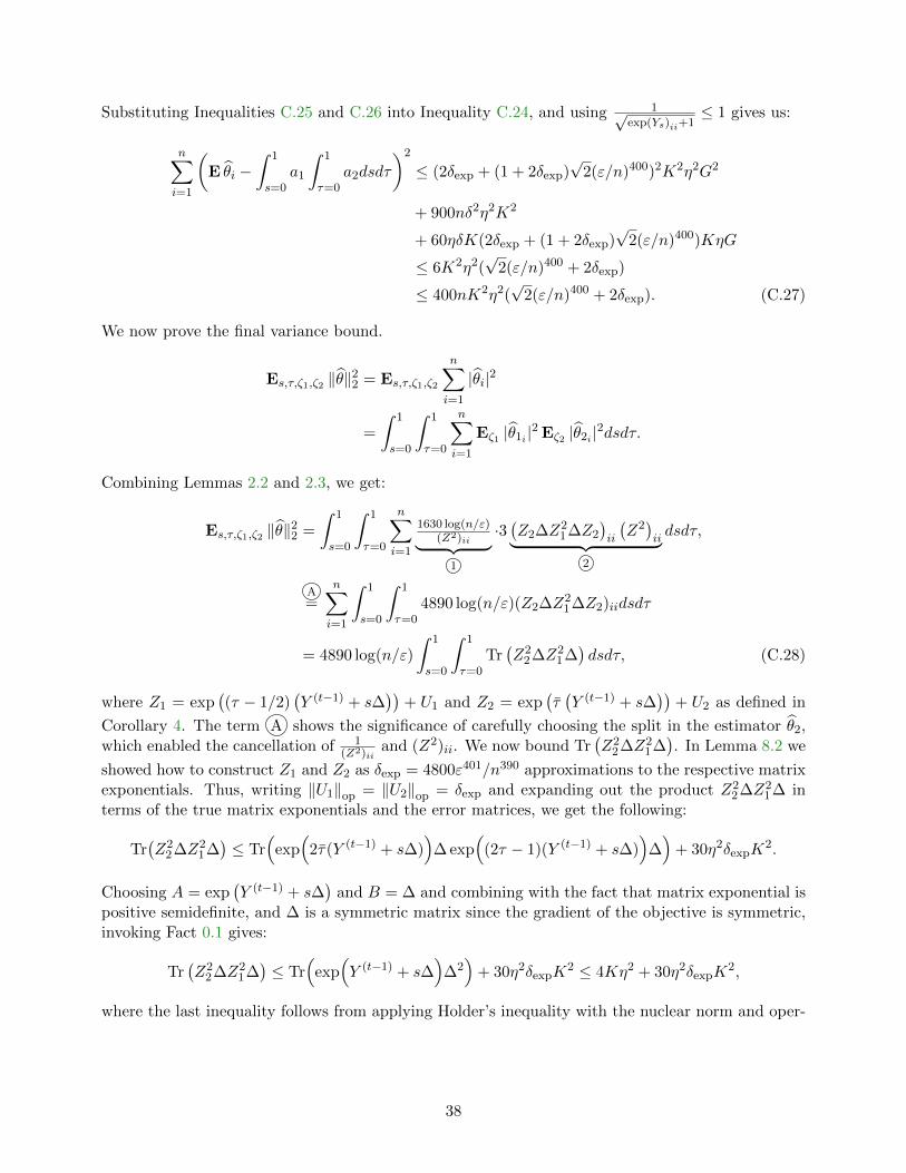
Substituting Inequalities C.25 and C.26 into Inequality C.24, and using 1√exp(Ys)ii+1

≤ 1 gives us:

n∑i=1

(E θi −

∫ 1

s=0a1

∫ 1

τ=0a2dsdτ

)2

≤ (2δexp + (1 + 2δexp)√

2(ε/n)400)2K2η2G2

+ 900nδ2η2K2

+ 60ηδK(2δexp + (1 + 2δexp)√

2(ε/n)400)KηG

≤ 6K2η2(√

2(ε/n)400 + 2δexp)

≤ 400nK2η2(√

2(ε/n)400 + 2δexp). (C.27)

We now prove the final variance bound.

Es,τ,ζ1,ζ2 ‖θ‖22 = Es,τ,ζ1,ζ2

n∑i=1

|θi|2

=

∫ 1

s=0

∫ 1

τ=0

n∑i=1

Eζ1 |θ1i |2 Eζ2 |θ2i |2dsdτ.

Combining Lemmas 2.2 and 2.3, we get:

Es,τ,ζ1,ζ2 ‖θ‖22 =

∫ 1

s=0

∫ 1

τ=0

n∑i=1

1630 log(n/ε)(Z2)ii︸ ︷︷ ︸

1

·3(Z2∆Z2

1∆Z2

)ii

(Z2)ii︸ ︷︷ ︸

2

dsdτ,

A=

n∑i=1

∫ 1

s=0

∫ 1

τ=04890 log(n/ε)(Z2∆Z2

1∆Z2)iidsdτ

= 4890 log(n/ε)

∫ 1

s=0

∫ 1

τ=0Tr(Z2

2∆Z21∆)dsdτ, (C.28)

where Z1 = exp((τ − 1/2)

(Y (t−1) + s∆

))+ U1 and Z2 = exp

(τ(Y (t−1) + s∆

))+ U2 as defined in

Corollary 4. The term A shows the significance of carefully choosing the split in the estimator θ2,which enabled the cancellation of 1

(Z2)iiand (Z2)ii. We now bound Tr

(Z2

2∆Z21∆). In Lemma 8.2 we

showed how to construct Z1 and Z2 as δexp = 4800ε401/n390 approximations to the respective matrixexponentials. Thus, writing ‖U1‖op = ‖U2‖op = δexp and expanding out the product Z2

2∆Z21∆ in

terms of the true matrix exponentials and the error matrices, we get the following:

Tr(Z2

2∆Z21∆)≤ Tr

(exp(

2τ(Y (t−1) + s∆))

∆ exp(

(2τ − 1)(Y (t−1) + s∆))

∆)

+ 30η2δexpK2.

Choosing A = exp(Y (t−1) + s∆

)and B = ∆ and combining with the fact that matrix exponential is

positive semidefinite, and ∆ is a symmetric matrix since the gradient of the objective is symmetric,invoking Fact 0.1 gives:

Tr(Z2

2∆Z21∆)≤ Tr

(exp(Y (t−1) + s∆

)∆2)

+ 30η2δexpK2 ≤ 4Kη2 + 30η2δexpK

2,

where the last inequality follows from applying Holder’s inequality with the nuclear norm and oper-

38

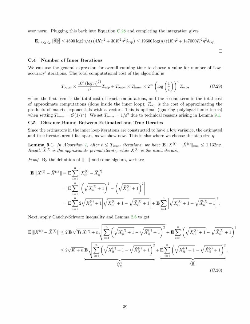
ator norm. Plugging this back into Equation C.28 and completing the integration gives

Es,τ,ζ1,ζ2 ‖θ‖22 ≤ 4890 log(n/ε)(4Kη2 + 30K2η2δexp

)≤ 19600 log(n/ε)Kη2 + 147000K2η2δexp.

C.4 Number of Inner Iterations

We can use the general expression for overall running time to choose a value for number of ‘low-accuracy’ iterations. The total computational cost of the algorithm is

Touter ×105 (log n)21

ε2Texp + Touter × Tinner × 230

(log

(1

ε

))4

Texp, (C.29)

where the first term is the total cost of exact computations, and the second term is the total costof approximate computations (done inside the inner loop); Texp is the cost of approximating theproducts of matrix exponentials with a vector. This is optimal (ignoring polylogarithmic terms)when setting Tinner = O(1/ε2). We set Tinner = 1/ε2 due to technical reasons arising in Lemma 9.1.

C.5 Distance Bound Between Estimated and True Iterates

Since the estimators in the inner loop iterations are constructed to have a low variance, the estimatedand true iterates aren’t far apart, as we show now. This is also where we choose the step size η.

Lemma 9.1. In Algorithm 1, after t ≤ Tinner iterations, we have E ‖X(t) − X(t)‖nuc ≤ 1.132nε.Recall, X(t) is the approximate primal iterate, while X(t) is the exact iterate.

Proof. By the definition of ||| · ||| and some algebra, we have

E |||X(t) − X(t)||| = En∑i=1

∣∣∣X(t)ii − X

(t)ii

∣∣∣= E

n∑i=1

∣∣∣∣∣(√

X(t)ii + 1

)2

−(√

X(t)ii + 1

)2∣∣∣∣∣

= E

n∑i=1

2

√X

(t)ii + 1

∣∣∣∣√X(t)ii + 1−

√X

(t)ii + 1

∣∣∣∣+ E

n∑i=1

∣∣∣∣√X(t)ii + 1−

√X

(t)ii + 1

∣∣∣∣2.Next, apply Cauchy-Schwarz inequality and Lemma 2.6 to get

E |||X(t) − X(t)||| ≤ 2 E√

TrX(t) + n

√√√√ n∑i=1

(√X

(t)ii + 1−

√X

(t)ii + 1

)2

+ E

n∑i=1

(√X

(t)ii + 1−

√X

(t)ii + 1

)2

≤ 2√K + nE

√√√√ n∑i=1

(√X

(t)ii + 1−

√X

(t)ii + 1

)2

︸ ︷︷ ︸A

+ E

n∑i=1

(√X

(t)ii + 1−

√X

(t)ii + 1

)2

︸ ︷︷ ︸B

.

(C.30)

39

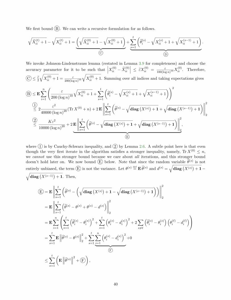
We first bound B . We can write a recursive formulation for as follows.

√X

(t)ii + 1−

√X

(t)ii + 1 =

(√X

(0)ii + 1−

√X

(0)ii + 1

)︸ ︷︷ ︸

C

+

t∑s=1

(θ

(s)i −

√X

(s)ii + 1 +

√X

(s−1)ii + 1

)︸ ︷︷ ︸

D

.

We invoke Johnson-Lindenstrauss lemma (restated in Lemma 3.9 for completeness) and choose the

accuracy parameter for it to be such that∣∣∣X(0)

ii − X(0)ii

∣∣∣ ≤ εX(0)ii = ε

100(logn)10X(0)ii . Therefore,

C ≤ ε2

√X

(0)ii + 1 = ε

200(logn)10

√X

(0)ii + 1. Summing over all indices and taking expectations gives

B ≤ En∑i=1

(ε

200 (log n)10

√X

(0)ii + 1 +

t∑s=1

(θ

(s)i −

√X

(s)ii + 1 +

√X

(s−1)ii + 1

))2

1≤ 2

ε2

40000 (log n)20 (TrX(0) + n) + 2 E

∥∥∥∥∥t∑

s=1

(θ(s) −

√diag

(X(s)

)+ 1 +

√diag

(X(s−1)

)+ 1

)∥∥∥∥∥2

2

2≤ Kε2

10000 (log n)20 + 2 E

∥∥∥∥∥t∑

s=1

(θ(s) −

√diag

(X(s)

)+ 1 +

√diag

(X(s−1)

)+ 1

)∥∥∥∥∥2

2︸ ︷︷ ︸E

,

where 1 is by Cauchy-Schwarz inequality, and 2 by Lemma 2.6. A subtle point here is that eventhough the very first iterate in the algorithm satisfies a stronger inequality, namely, TrX(0) ≤ n,we cannot use this stronger bound because we care about all iterations, and this stronger bounddoesn’t hold later on. We now bound E below. Note that since the random variable θ(s) is not

entirely unbiased, the term E is not the variance. Let θ(s) def= E θ(s) and d(s) =

√diag

(X(s)

)+ 1−√

diag(X(s−1)

)+ 1. Then,

E = E

∥∥∥∥∥t∑

s=1

(θ(s) −

(√diag

(X(s)

)+ 1−

√diag

(X(s−1)

)+ 1

))∥∥∥∥∥2

2

= E

∥∥∥∥∥t∑

s=1

(θ(s) − θ(s) + θ(s) − d(s)

)∥∥∥∥∥2

2

= E

n∑i=1

t∑s=1

(θ

(s)i − θ

(s)i

)2+

t∑s=1

(θ

(s)i − d

(s)i

)2+ 2

∑s6=`

(θ

(s)i − θ

(s)i

)(θ

(`)i − d

(`)i

)=

t∑s=1

E∥∥∥θ(s) − θ(s)

∥∥∥2

2+

t∑s=1

n∑i=1

(θ

(s)i − d

(s)i

)2

︸ ︷︷ ︸F

+0

≤t∑

s=1

(E∥∥∥θ(s)

∥∥∥2+ F

),

40

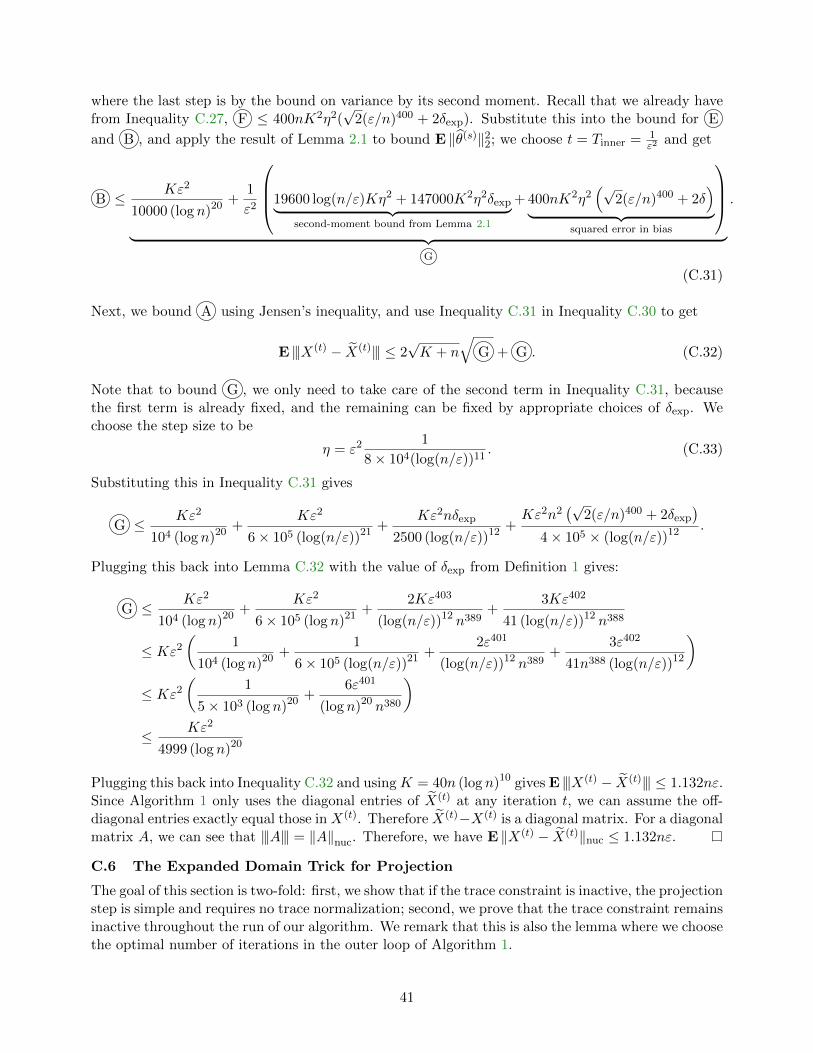
where the last step is by the bound on variance by its second moment. Recall that we already havefrom Inequality C.27, F ≤ 400nK2η2(

√2(ε/n)400 + 2δexp). Substitute this into the bound for E

and B , and apply the result of Lemma 2.1 to bound E ‖θ(s)‖22; we choose t = Tinner = 1ε2

and get

B ≤ Kε2

10000 (log n)20 +1

ε2

19600 log(n/ε)Kη2 + 147000K2η2δexp︸ ︷︷ ︸second-moment bound from Lemma 2.1

+ 400nK2η2(√

2(ε/n)400 + 2δ)

︸ ︷︷ ︸squared error in bias

︸ ︷︷ ︸

G

.

(C.31)

Next, we bound A using Jensen’s inequality, and use Inequality C.31 in Inequality C.30 to get

E |||X(t) − X(t)||| ≤ 2√K + n

√G + G . (C.32)

Note that to bound G , we only need to take care of the second term in Inequality C.31, becausethe first term is already fixed, and the remaining can be fixed by appropriate choices of δexp. Wechoose the step size to be

η = ε2 1

8× 104(log(n/ε))11. (C.33)

Substituting this in Inequality C.31 gives

G ≤ Kε2

104 (log n)20 +Kε2

6× 105 (log(n/ε))21 +Kε2nδexp

2500 (log(n/ε))12 +Kε2n2

(√2(ε/n)400 + 2δexp

)4× 105 × (log(n/ε))12 .

Plugging this back into Lemma C.32 with the value of δexp from Definition 1 gives:

G ≤ Kε2

104 (log n)20 +Kε2

6× 105 (log n)21 +2Kε403

(log(n/ε))12 n389+

3Kε402

41 (log(n/ε))12 n388

≤ Kε2

(1

104 (log n)20 +1

6× 105 (log(n/ε))21 +2ε401

(log(n/ε))12 n389+

3ε402

41n388 (log(n/ε))12

)≤ Kε2

(1

5× 103 (log n)20 +6ε401

(log n)20 n380

)≤ Kε2

4999 (log n)20

Plugging this back into Inequality C.32 and usingK = 40n (log n)10 gives E |||X(t) − X(t)||| ≤ 1.132nε.Since Algorithm 1 only uses the diagonal entries of X(t) at any iteration t, we can assume the off-diagonal entries exactly equal those in X(t). Therefore X(t)−X(t) is a diagonal matrix. For a diagonalmatrix A, we can see that |||A||| = ‖A‖nuc. Therefore, we have E ‖X(t) − X(t)‖nuc ≤ 1.132nε.

C.6 The Expanded Domain Trick for Projection

The goal of this section is two-fold: first, we show that if the trace constraint is inactive, the projectionstep is simple and requires no trace normalization; second, we prove that the trace constraint remainsinactive throughout the run of our algorithm. We remark that this is also the lemma where we choosethe optimal number of iterations in the outer loop of Algorithm 1.

41

Lemma 9.2. Consider the mirror map Φ(X) = X•logX−TrX over the domain X : X 0,TrX ≤K. Assuming that the trace inequality is never active, we have that expY = argminX0,TrX≤K Φ(X)−Y •X.

Proof. We wish to solve

minX • logX − TrX −X • Y, subject to X 0,TrX ≤ K. (C.34)

By diagonalizing X as X = UΛU> and Y as Y = V ΣV >, we can rewrite this problem as

minn∑i=1

λi log λi −n∑i=1

λi −n∑i=1

λiyi, subject to λi ≥ 0,n∑i=1

λi ≤ K, (C.35)

where yi is the i’th diagonal entry of the matrix U>Y U . The Lagrangian is given by L(λi, ν) =∑ni=1 λi log λi −

∑ni=1 λi −

∑ni=1 λiyi + ν (

∑ni=1 λi −K). Setting the gradient to zero gives ∇ΛL =

1 + log λ∗ − 1− y + ν1 = 0, which gives λ∗i = exp(yi − ν) for all i. Since we assumed that the traceconstraint is not active, it means, by complementary slackness, ν = 0 (note that this assumption isjustified because we prove it in Lemma 2.6). This gives λ∗i = exp(yi) which translates toX∗ = exp(Y ),as claimed.

Before we start the second proof, we need the following result.

Lemma 9.3. Fix a norm ‖ · ‖. Given an α-strongly convex mirror map Φ : D → R, a convex,

G-Lipschitz objective f : X → R, the diameter of X ∩D denoted by Ddef= sup

x∈X∩DΦ(X)− inf

x∈X∩DΦ (x),

step size η, and parameter δ′ where E∥∥x(t) − x(t)

∥∥ ≤ δ′, running mirror descent for T iterations

gives iterates x(t)Tt=1 that satisfy the inequality

f

(1

T − 1

T−1∑t=1

x(t)

)− f (x∗) ≤ ηG2

2α+

1

η (T − 1)(DΦ(x∗, x(1))−DΦ(x∗, x(T ))) + δ′G.

This can be derived the same way as Theorem 4.2 in [B+15], by incorporating the error in iterate,just as we did in the proof of Theorem 1.

Lemma 2.6. With the choice of parameters in Algorithm 1, the iterate X(t) at any iteration tsatisfies Tr X(t) < K for K = 40n(log n)10.

Proof. We prove this by induction on the iteration count.Induction Hypothesis. We assume that for any iteration t, the primal iterate is not too far

from the optimal point, satisfying |||X(t) −X∗||| ≤ 38n (log n)10.Base Case. Since Y (1) = 0, the primal iterate X(1) = I. We also know that the optimal point

satisfies TrX∗ = n. Therefore, |||X(1) −X∗||| ≤ 2n ≤ 38n (log n)10. The hypothesis is thus true forthe base case, t = 1.

Induction. Suppose that the hypothesis is true for some t = t′. We prove that this wouldmake it true for t = t′ + 1 as well. Our technique is to first prove a weak bound for |||X(t) −X∗|||using triangle inequality of norms; then we boost our bound (and obtain the stronger guarantee ofthe induction hypothesis) by invoking strong convexity of Bregman Divergence. We now show the

42

details.

|||X(t′+1) −X∗||| ≤ |||X(t′+1) − X(t′)|||+ |||X(t′) −X∗|||

≤∥∥∥X(t′+1) − X(t′)

∥∥∥nuc︸ ︷︷ ︸

Inequality A.6

+ |||X(t′) −X∗|||︸ ︷︷ ︸induction hypothesis

.

≤ 2ηG

α︸︷︷︸A

+38n (log n)10 . (C.36)

The first step here used the fact that |||M ||| ≤ ‖M‖nuc(We can show this by Holder’s Inequality,〈X,Y 〉 ≤ ‖Y ‖op‖X‖nuc. Select Y = diag (sgn (diagX)), that is, Y is a diagonal matrix withYii = sgn (Xii)). We can plug in parameters of the mirror map and the step size, as displayed inTable 1, to obtain:

A = 2 · ε2

80000(log(n/ε))11· 2 · 4(40n(log n)10) ≤ nε2

125.

Plugging this back into Equation C.36 while using ε < 1/2 andK = 40n(log n)10 gives |||X(t′+1) −X∗||| ≤nε2

125 +38n (log n)10, which implies that Tr(X(t′)

)< (n(ε2/125+38(log n)10)+n) < 40n(log n)10 = K,

which says that the trace constraint on the iterates is not active on the first t′ iterations.Since the trace constraint is not active on the first t′ iterations, the projection step does not

require a normalization. This implies that Algorithm 3 now is identical to Approximate MirrorDescent with this mirror map and objective. We now recall Lemma 9.3 for T = t′ + 1:

f

(1

t′

t′∑t=1

X(t)

)− f (X∗) ≤ ηG2

2α+

1

ηt′(DΦ(X∗, X(1))−DΦ(X∗, X(t′+1))) + δ′G.

Multiplying throughout by ηt′ and rearranging the terms gives

DΦ(X∗, X(t′+1)) ≤ η2G2t′

2α+DΦ(X∗, X(1))− ηt′

(f

(1

t′

t′∑t=1

X(t)

)− f (X∗)

)︸ ︷︷ ︸

positive

+ηt′δ′G (C.37)

Since Φ is α-strongly convex in the nuclear norm, we have DΦ(X∗, X) ≥ α2 ‖X

∗ − X‖2nuc. Since this

is at least α2 |||X

∗ − X|||2. Chaining this with Inequality C.37 gives

|||X(t′+1) −X∗|||2≤ η2G2t′

α2︸ ︷︷ ︸B

+2DΦ(X∗, X(1))

α︸ ︷︷ ︸C

+2

αηt′δ′G︸ ︷︷ ︸

D

, (C.38)

We now bound each of the terms on the right-hand side. We remark that this is actually where we

43

choose the appropriate value of Touter.

B =η2G2TinnerTouter

α2

=ε4

64× 108 (log(n/ε))22 · 4 ·1

ε2· 1

ε24× 105 (log(n/ε))11 log n · 16

(40n (log n)10

)2

≤ 40εn2 (log n)10

To bound the second term C = 2DΦ(X(1),X∗)α , we need to compute DΦ(X(1), X∗). Recall that

X(1) = I by our algorithm. Therefore, Φ(X(1)) = −n and ∇Φ(X(1)) = 0. Applying Holder’sinequality gives Φ(X∗) ≤ TrX∗ log ‖X∗‖op ≤ n log n. Therefore DΦ(X∗, X(1)) ≤ n log n. Now we goback to the quantity we were trying to bound:

C ≤ 2 · n log n · 4(40n(log n)10) ≤ 320n2 (log n)11 .

Finally, the last term is:

D =2

αηTinnerTouterδ

′G ≤ 2 · 4K · 30 log n

ε· 1.132nε · 2 = 21735n2 (log n)11

Summing these terms and plugging back into Inequality C.38 gives

|||X(t′+1) −X∗|||2≤ n2(40ε(log n)10 + 320(log n)11 + 21735(log n)11).

< n2(0.77(log n)20 + 17(log n)20 + 1150(log n)20)

≤ 1168n2 (log n)20 ≤ 35n (log n)10 ,

which completes the induction. Therefore we have |||X(t) −X∗||| ≤ 38n (log n)10 for all t. SinceTrX∗ = n, this proves Tr X(t) < 40n (log n)10 = K.

C.7 Error bound

Finally, we put together all the parameters derived above to obtain our claimed error bound.

Lemma 9.4. Running Algorithm 1 gives an output for (1.2) that has an error bound of Kε.

Our algorithm is in the framework of approximate lazy mirror descent, with error bound givenby Theorem 1, restated below.

Theorem 1 (Convergence of Lazy Mirror Descent). Fix a norm ‖ · ‖. Given an α-strongly convexmirror map Φ : D → R and a convex, G-Lipschitz objective f : X → R, run Algorithm 3 with stepsize η and E ‖x(t) − x(t)‖ ≤ δ. Let D

def= supx∈X∩D Φ (x) − infx∈X∩D Φ (x). Then, Algorithm 3 after

T iterations returns xt∗, satisfying

E f(x(t∗))− f (x∗) ≤ D

Tη+

2ηG2

α+ δG. (1.6)

Proof. Our proof involves plugging in the values of the parameters (from Table 1) in the above

44

bound. Since we assume n ≥ 4, we use log n ≤√n in one of the calculations below.

D

Tη= Kε

logK

30 log n≤ Kε log 40 + 6 log n

30 log n≤ 0.29Kε.

2ηG2

α=

32ε2K

8× 104 (log n)11 =Kε

2500 (log n)11 ≤ 2× 10−5Kε

δG = 1.132nε ≤ Kε

35 (log n)10 ≤ 11× 10−4Kε

Summing these quantities gives the upper bound on the error to be εK, as claimed.

D General Technical Results

Lemma 9.1. Given a, b ∈ Rn , we have that Eζ∼N (0,I)

((ζTa)2(ζT b)2

)≤ 3‖a‖22‖b‖

22.

Proof. By Cauchy-Schwarz inequality, the functions f1 and f2 satisfy Eζ∼N (0,I)(f1 (ζ) f2 (ζ)) ≤√Eζ(f1 (ζ))2 Eζ(f2 (ζ))2. Choose f1 (ζ) = (ζTa)2 and f2 (ζ) = (ζT b)2. Since ζ ∼ N (0, I) and

all the coordinates of ζ are independent, Var(ζTa) =∑n

i=1 Var(ζiai) =∑n

i=1 a2i = ‖a‖22. Therefore

ζTa ∼ N (0, ‖a‖22). For X ∼ N (0, σ2), we have EX4 = 3σ4. Applying this to ζTa and ζT b provesthe desired inequality.

45