WORKING PAPER SERIES 07-2016

Πατησίων 76, 104 34 Αθήνα. Tηλ.: 210 8203303-5 / Fax: 210 8238249

76, Patission Street, Athens 104 34 Greece. Tel.: (+30) 210 8203303-5 / Fax: (+30) 210 8238249 E-mail: econ@aueb.gr / www.aueb.gr

Optimal Bailout of Systemic Banks

Charles Nolan , Plutarchos Sakellaris and John D. Tsoukalas

Optimal Bailout of Systemic Banks ∗

Charles NolanUniversity of Glasgow

Plutarchos SakellarisAthens University of Economics and Business

John D. TsoukalasUniversity of Glasgow

September 2016

Abstract

Following the recent global financial crisis, there have been many sig-nificant changes to financial regulatory policies. These may have re-duced the likelihood and future cost of the next crisis. However, theyhave not addressed the central dilemma in financial regulation whichis that governments cannot commit not to bail out banks and other fi-nancial firms. We develop a simple model to reflect this dilemma, andargue that some form of penalty structure imposed on key decision-makers post-bailout is necessary to address it.

Keywords: Financial Crisis, Bank bail-outs, Systemic risk, Macropru-dential policy.

JEL Classification: E2, E3.

∗We thank seminar participants at various institutions. Nolan: University of Glas-gow, Adam Smith Business School/Economics, Main Building, Glasgow, G12 8QQ.Email: charles.nolan@glasgow.ac.uk. Sakellaris: Athens University of Economics andBusiness, Athens, 104 34. Email: plutarch@aueb.gr. Tsoukalas: University of Glas-gow, Adam Smith Business School/Economics, Main Building, Glasgow, G12 8QQ. Email:john.tsoukalas@glasgow.ac.uk.

1

1 Introduction

The central problem in financial regulation is that governments cannot

commit not to bail out banks and other financial firms. The recent financial

crisis pushed some governments to the brink of insolvency in dramatic

confirmation of this. As noted recently by Mervyn King, former Governor of

the Bank of England:

When all the functions of the financial system are so closely

interconnected, any problems that arise can end up playing

havoc with services vital to the operation of the economy - the

payments system, the role of money and the provision of working

capital to industry. If such functions are materially threatened,

governments will never be able to sit idly by. Institutions

supplying those services are quite simply too important to fail.

Everyone knows it. (King (2016), p. 96)

And the resulting moral hazard problem is widely acknowledged:

Greater risk begets greater size, greater importance to the

functioning of the economy, higher implicit public subsidies, and

yet larger incentives to take risk. (King, op. cit.)

Following the recent financial crisis governments and regulators across

the world made coordinated efforts to increase capital and liquidity in the

banking system, to reform resolution procedures for restructuring failed

banks, to identify systemically important financial institutions and to think

through supervision of hitherto less regulated areas of the financial sector

(such as shadow banks).1 Some countries have pursued additional reforms

chipping away at the universal banking business model, tightening ‘fitness

1Many of these initiatives have flowed from the Basel Committee on BankingSupervision and the Financial Stability Board.

2

and properness’ procedures around identified key posts, altering pay and

bonus structures, introducing lending limits and leverage ratios, and many

other reforms besides2. Finally, there has been much interest in so-called

macroprudential regulation and some countries have set up macroprudential

authorities with, in principle, wide-ranging powers.

When all these reforms are fully in place, will bailouts be so unlikely as

to not materially distort financial sector behaviour? We argue that whilst

many of these reforms are desirable, there are good grounds for believing that

the central problem of financial regulation remains unsolved. The reason is

simple: None of the reforms make time-consistent the promise not to bail

out banks and other systemically important institutions (‘banks’ for short).

The essence of the time consistency problem, as the quote above from King

(2016) indicates, is that banks have an important role in the economy. They

provide ‘money’, effect payments, fund working capital, and indeed they are

vehicles to take over other, weaker institutions in times of stress. None of the

reforms change this fundamentally. And indeed, none were designed so to

do. They were designed, in effect, to reduce the cost to the taxpayer of the

next bailout. That is the thinking behind increased capital requirements and

related balance sheet rules imposed on banks. For example, a leverage ratio,

even when respected, can still permit excessively risky lending at the margin

and in difficult economic times it may well be optimal for policymakers to

ditch leverage ratios to recover wider economic stability.3

We argue instead that it is important to try to address the bailout/moral

hazard problem directly. We propose that regulators ought also to implement

post-bailout penalties on bankers. In acknowledging that bailouts will be

necessary from time to time, policymakers are accepting the inevitable, as

noted by King (2016). However, unlike the leverage ratio example, levying

2It is worth mentioning stress tests and so-called living wills.3This is an example of what King calls the ‘policy paradox’; what is optimal in the

short run is precisely the opposite of what is required in the long run.

3

penalties on bankers whose bank has been bailed out is time consistent. It

will be in the interests of policymakers to implement such penalties and as

such it will be in the interests of bankers to internalize those penalties ex ante.

Rather than have exogenously imposed, time inconsistent regulations at the

margin to discourage institutions from becoming systemically important,

such penalties would credibly induce banks to become less systemically

important. This proposal works with the grain of, and extends, recent policy

developments notably the formal designation of certain financial firms as

systemically important and innovations such as the Senior Managers Regime

in the UK4. Towards the end of the paper we conjecture how such penalties

might work in practice.

1.1 How big is the ”too big to fail” problem?

Costs to taxpayers of bank bailouts have been substantial during the financial

crisis that started in 2007. For example, in the U.S. gross Federal outlays

and explicit guarantees for financial system support amounted to $3.7 trillion

as of June 30th, 2010 (Table 3.1, SIGTARP Quarterly Report to Congress,

July 2010). Part of this exposure was collateralized and much has been

repaid to date. To get an idea of funded outlays, $414 billion had actually

been expended as part of the U.S. governments TARP program by the end of

2011. The costs of interventions in the financial sector following the recent

crisis have been large in Europe as well. The magnitude of the financial

resources needed by euro area governments from 2008 to 2013 to provide the

financial support was 5.1% of GDP (see Maurer and Grussenmeyer (2015)).

As a comparison, the analogous figure for the U.K. over the same period was

4The Financial Stability Board and the Basel Committee on Banking Supervisiondesignate certain institutions as systemically important. As a result they are supervisedmore closely and have higher prudential capital requirements, the more so the more riskythey are perceived to be. There has also been a renewed focus on important decisionmakers in regulated institutions, such as the regime in the UK noted in the main text.These schemes, and related changes to compensation packages, are unrelated to systemicbailouts in the way we will argue is necessary.

4

6.3% of GDP. The hardest-hit governments were Ireland (37.3% of GDP)

and Greece (24.8% of GDP). Not all of these amounts may be counted as

eventual losses, however. Maurer and Grussenmeyer (2015) estimate the

expected losses to euro area governments at 1.7% of GDP up to 2013 and

correspondingly, to 2.2% of GDP for the U.K. (see their Table 5). Similar

fiscal costs in a broader sample of countries that experienced financial crisis

during 1970-2011 are reported in Laeven and Valencia (2013).

There is substantial evidence that banks that are considered to be

systemic enjoy an advantage in the equity market compared to the rest of

the banking system. Some papers provide quantitative estimates of such

implicit subsidies. OHara and Shaw (1990) conduct an event study of a

public statement by the US Comptroller of the Currency in 1984 concerning

the need to provide full deposit insurance to some unspecified banks that

were “too-big-to-fail”. The Wall Street Journal went further and identified

the banks to which it considered the Comptroller was referring. OHara and

Shaw (1990) find that the Comptrollers announcement did not have distinct

effects on the banks based on an assessment of their solvency. However,

70% of the banks identified by the Wall Street Journal as systemic displayed

positive excess returns, whereas only 37% of the rest of the banks did so.

Kelly et al. (2016) document the divergence of individual and index put

prices during the recent financial crisis and provide evidence that a sector-

wide bailout guarantee in the financial sector was largely responsible for that.

They obtain a dollar estimate of the value of the government guarantee for

the financial sector. Specifically, government support to banks equity was

$0.63 billion before mid-2007 and rose to $42.38 billion between mid-2007

and mid-2009. It peaked at over $150 billion. Gandhi and Lustig (2015),

in a study of equity returns between 1970 and 2005, found that large banks

yielded risk-adjusted returns that were 5% per annum lower than those of

the smallest banks. They attributed this difference to an implicit government

guarantee that absorbs the tail risk of large banks.

5

The International Monetary Funds Global Financial Stability Report for

April 2014 (see Fund (2014)) empirically captures the implicit subsidy to

large Systemically Important Banks (SIBs) resulting from the expectation

of government support in case of distress. They use three methods: 1) the

difference in bank bond spreads, 2) a contingent claims analysis (CCA),

and 3) a credit ratings approach. These methodologies have significant

differences, each with its own advantages and drawbacks, but they all

qualitatively result in positive implicit subsidies for SIBs. In particular, the

CCA estimates suggest that in the advanced economies, implicit subsidies

for SIBs averaged around 30 basis points over 2005 2014. The subsidies

increased temporarily during the financial crisis, climbing to around 60 basis

points in 2009. The subsidies grew again later on with the rise of European

sovereign stress.

1.2 The argument in more detail

We consider a simple model with an important banking sector and a

government that may end up having to meet bank losses–the central problem

noted above. The model builds on Damjanovic et al. (2013). Banks are

needed to channel working capital to firms who may or may not be able to

repay those loans. Because the government stands ready to offer a bailout,

banks lend more than they would in a competitive equilibrium without

bailouts. Bailouts are costly in part as they are funded by distortive labour

taxes.5

We assume bankers are risk averse and take the benchmark, constrained

efficient equilibrium in the model to be one where governments can commit

not to bail banks out.6 Because governments can commit, banks never go

5We also consider what impact there might be when there are limits to how much fiscalheadroom the government has. These so-called ‘fiscal limits’ have been much studied inrecent years.

6We call this the constrained efficient equilibrium as we take the nature of financialcontracts and the existence of banks as given. Hence, we presume, banks and contracts

6

bust so as to ensure bankers never experience negative consumption. So,

bankers optimally respect, in effect, a self-imposed solvency constraint. Since

banks never go bust, distortive labour taxes are never levied on private

agents. As noted, this is the constrained efficient equilibrium of the model.

However, such government commitment in the model is incredible since

banks are necessary for production of the final good. Since bankers’ expected

consumption is at least as high with bailouts as without, they are likely to

undertake lending policies that expose the government to the banks’ default

risk. Many regulatory restrictions might be placed on banks to cope with

this situation. In time-consistent equilibria, externally-imposed solvency

constraints or leverage constraints are neither necessary nor sufficient to

improve outturns. The problem with a solvency constraint in our model

is that is not time consistent. The banker will ignore it and enjoy higher

consumption if they do.

Being unable to dispense with banks, the government can replicate the

constrained efficient allocation–the competitive equilibrium with no default–

by imposing a consumption penalty on bankers if a bailout has ever occurred.

The reason why the penalty function is time-consistent is because it accepts

that the bailout will happen if a default occurs and it is optimal to impose

it. The penalty in the model is a function of aggregate state variables; in the

present model these are government debt, which reflects any past bailouts

that may have occurred. The government cannot credibly commit not to

bail out the banks but it can credibly commit to execute the penalty. The

consumption penalty levied today is the present value of the bailout plus a

surcharge that accounts for social cost of the bailout.7 That cost is driven

by the distortion in labor supply caused by labor taxes. So the penalty

is a function of Bt which summarizes all the past bailouts and At which

reflect an efficient, competitive response to some deeper asymmetric information or moralhazard problem. Such an assumption is common in macro-banking analyses.

7In the model, the surcharge is necessary to avoid an indeterminacy; if the banker onlypaid for the direct monetary cost she may be indifferent to default.

7

determines the size of the current bailout. No other macro prudential policy

appears able to deliver the constrained efficient equilibrium, because they are

time inconsistent. The penalty makes bankers internalize the moral hazard

problem by being contingent on aggregate states.

It could well be that the government is unable to raise sufficient tax

revenues to bail the banks out. In that event bond holders may have to bear

some cost. As a result future fiscal capacity rises and the penalty has to

take the form of a consumption tax surcharge so that the bankers internalize

the cost to bondholders. And the government then has the option of debt

reschedule in effect what the bankers will pay back in due course.

There are several interesting implications of our set up. Suppose there

was a leverage ratio to take the economy closer to the competitive time-

consistent equilibrium. A central finding is that leverage ratio should be a

function not only of bank-specific variables, but also of the government’s fiscal

capacity. That latter finding is not apparent in any proposals put forward

so far under the guise of macro-prudential regulation. Moreover, periods of

low government debt, absent the optimal bank levy just described, encourage

banks to expand excessively. Periods of high fiscal capacity can encourage

credit booms. Finally, following a bailout so long as the government is

credibly implementing penalties, financial crisis are less likely to happen,

first because the governments have less fiscal capacity, and second because

banks wish to avoid additional penalties on top of those just levied.

In short, then, we demonstrate two things. First, that the optimal time–

consistent macro prudential policy that replicates an equilibrium with no

bailouts and zero debt, is like a tax on bankers consumption and contingent

on aggregate states; an important such state is governments’ fiscal capacity

which itself is a function of existing debt. That removes the incentive

of bankers to take excessive risk because it makes them internalize the

cost of bailouts. We also show that policies such as solvency or leverage

constraints are sub-optimal because they are time inconsistent just at the

8

point when governments and regulators confront the central problem of

financial regulation. The government cannot commit not to bail out bankers

with those policies in place. It follows that the non–zero correlations between

credit spreads and bond spreads observed during periods of financial crisis

reflect suboptimal government policies that do not remove bankers’ incentive

to take excessive risks.

2 Literature and policy overview

The present paper contributes to a now large literature on macroprudential

regulation. Duncan and Nolan (2015) is a review of recent policy

developments. They argue that the literature has focussed on four

key externalities which macroprudential policy confronts. First, there

are the balance sheet externalities emphasized by Bernanke et al.

(1999) and Kiyotaki and Moore (1997). Next, there are the monetary

transmission/aggregate demand externalities highlighted by Friedman and

Schwartz (1963) and Farhi and Werning (2013). Third, there are herding

externalities studied in Duncan (2015). And finally, there are bailout

externalities associated with the too-big-to-fail problem analyzed, for

example, in Haldane (2012), the focus of this paper.

A central issue which macroprudential policy must confront is that these

externalities, not all of them concentrated in the more regulated areas of

the financial sector, interact with one another and with microprudential

regulations blurring boundaries. Thus, time-varying capital requirements

or lending restrictions centred on banksfor some the defining characteristic

of macroprudential policy are at best insufficient in addressing the impact of

these and other externalities. For instance, balance sheet recessions are likely

to be costly even if monetary policy is unconstrained by the zero lower bound

(ZLB). However, that externality is much more serious when the monetary

transmission mechanism is dysfunctional (Friedman and Schwartz (1963),

9

Farhi and Werning (2013) and Schmitt-Grohe and Uribe (2012)). Of course,

some monetary policy innovations (such as QE/Forward Guidance/removal

of the ZLB) can work to offset some of these aggregate demand externalities

but in all likelihood other measures are likely required. However, additional

measures, including (statutory and extraordinary) deposit protection and

central bank/taxpayer assistance entail serious incentive costs exacerbating

the too-big-too-fail (TBTF) problem and herding effects. Moreover, these

too-big-too-fail and herding effects are in turn likely to feed back and

exacerbate the fire-sale, or balance-sheet, externality.

This complexity facing policymakers has led some economists to look for

simpler ways to address the fundamental problems as they see them. One way

is via the tax system. Jeanne and Korinek (2010) and Jeanne and Korinek

(2014) argue that there is a limit to the effectiveness of macroprudential

regulation focussed largely on banks and that discouraging borrowing via

the tax system may be more efficacious. Farhi and Werning (2013) suggest

that by discouraging debt, policymakers can make it more likely that the

ZLB binds so that monetary policy may stay more effective for longer during

financial recessions. Correia et al. (2013) make a similar point and show

that coordinated taxes on labour and consumption can mimic the effect

of negative nominal rates. Mendoza and Bianchi (2010) and Mendoza and

Bianchi (2013), study optimal time consistent policy in models that feature

the balance sheet externality and argue for state contingent taxes on debt

that reduce the incentives of agents to overborrow during good times, in effect

internalizing the externality. Their quantitative exercise suggests that the

debt tax can reduce the magnitude and frequency of financial crisis. These

and other examples all imply a possibly important role for the tax system. In

a similar setting, Bianchi (2012) studies optimal liquidity assistance (referred

to as a bailout) during credit crunch periods, when firms are undercapitalized,

in an attempt to relax balance sheet constraints. Mendoza and Bianchi (2015)

incorporate two key sources of volatility and credit cycles in the analysis of

10

macroprudential policy, namely noisy news about fundamentals and global

shifts in liquidity.

The importance of institutions (banks and others) that are too-big-too-fail

(TBTF) has been an important theme since the crisis unfolded. The policy

consensus that has emerged is that systemically important institutions should

be discouraged but nevertheless allowed to continue. More specifically, the

policy response to TBTF has included (proposed) increases in capital and

liquidity requirements via Basel III, Global Systemically Important Bank

(GSIB) capital surcharges, Pillar 2 increases and resolution-related capital

buffers. In addition to these, in the UK there has also been structural

reform (following the Vickers ring-fencing proposals). Some politicians and

regulators appear to believe we are now close to solving the TBTF problem

and that reforms to resolution have been key to this (Cunliffe (2014)). So,

important progress has been made: there is more and better capital and

liquidity in the banking sector; GSIBs have been identified and will be

supervised more stringently; a roadmap, agreed across countries, has been

approved on how to resolve these banks in case of trouble.

However, there remain doubts as to whether the TBTF problem has really

been solved. Although the changes just mentioned have made banks safer

one has to set these in context. The banking sector across many jurisdictions

has become more concentrated since the financial crisis, partly as a result

of bank bailouts. Governments and central banks bailed out more than

just banks and guaranteed liabilities somewhat wider than those covered

by deposit protection schemes. Moreover, if a systemically important bank

needs to be resolved, experience suggests that a number of other institutions

are likely to be in trouble at the same time. The question then is whether,

during a period when liquidity and solvency difficulties become indistinct,

the national Resolution Authorities will be able to conclude that recovery

is not feasible across a number of (doubtless interlinked) institutions and

markets and hence that they should each be resolved with no disruption to

11

the rest of the financial system.

It may then seem that big banks should simply be broken up. There

appears to be scepticism about this and policymakers revealed preference

has been largely to reject such an approach. There are arguments that

breaking up banks into smaller units may neither be desirable nor feasible.

Damjanovic et al. (2013) outline a macro-banking model whereby a trade-

off exists between larger universal banks which lend more, crash relatively

infrequently but at greater cost to the taxpayer, versus a smaller, less risky

and less profitable banking sector (split between retail and investment banks)

that lends less, crashes more frequently but at less cost to the taxpayer.

The welfare judgement turns on a complex interaction between common and

idiosyncratic financial shocks and pre-existing distortions in the economy. If

the economy is quite distorted (and hence has a low natural rate of output),

and financial shocks are not too large, then universal banks may be preferable

as they offset low average output. On the other hand, the banking sector

can be too big when dominated by universal banks. It is difficult to judge

which version of the model is more realistic. Some have argued that returns

to scale in banking are larger than traditional analyses suggest (although it

is hard to control for implicit bail out subsidies). Banks themselves tend to

argue that size and universality brings benefits in terms of risk-smoothing and

economies of scope. Others (e.g., Basu and Dixit (2014)) have pointed out

that breaking banks up may be costly and futile from a regulatory point of

view as it is difficult to levy penalties on small competitive banks with limited

liability. If lots of smaller banks adopted correlated investment strategies

and were less profitable than a smaller number of bigger banks, then it could

well be that financial crisis would be harder to deal with than under the

status quo (Chari and Phelan (2014), Duncan (2015) and Farhi and Tirole

(2012) present models of the interaction between financial sector herding

and stabilization policies). Finally, it has been argued that the existence of

big banks is ultimately a political decision; they may be seen as national

12

champions individually or collectively and as a good source of tax revenue in

tranquil times. On this view, TBTF will end when politicians decide it will

end. The existence of big banks and their political influence is documented

in a recent book (Calomiris and Haber (2014)) through history and across

countries.

Thus, it is not clear to us that the TBTF has been solved. We suggest

here that a better approach to the TBTF problem is to define ex ante how

the authorities will act ex post, having bailed out an institution. Whilst

shareholders are typically wiped out, one notes that few bank executives

suffer as a result of their institutions receiving taxpayers money. As a result,

remuneration schemes internal to banks do not attenuate the moral hazard

problem. Designing schemes that do attenuate this problem and hence

address directly the central problem in financial regulation is the subject

of this paper.

3 The Model

The model has a household sector, a final goods sector, a financial sector

and a government. There is a single homogenous final good produced using

labour. There are three household types, workers, investors, and bankers.

Final goods firms require working capital loans to finance production. These

loans are obtained from banks. The banks finance the loans from household

deposits and bank equity.

3.1 Households

The first type of household comprises workers who maximize,

E0

∞∑t=0

βt

[v(Ca

t ) + φ lnLt

], β ∈ (0, 1), φ > 0.

E0 is the conditional expectation operator, β is the discount factor, v′ >

0, v′′ < 0, while φ is the leisure weight parameter.

13

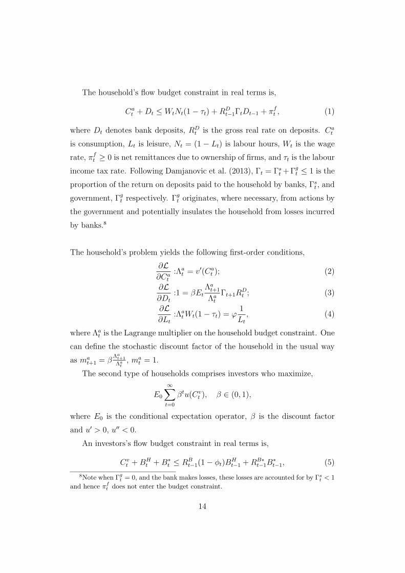
The household’s flow budget constraint in real terms is,

Cat +Dt ≤ WtNt(1− τt) +RD

t−1ΓtDt−1 + πft , (1)

where Dt denotes bank deposits, RDt is the gross real rate on deposits. Ca

t

is consumption, Lt is leisure, Nt = (1 − Lt) is labour hours, Wt is the wage

rate, πft ≥ 0 is net remittances due to ownership of firms, and τt is the labour

income tax rate. Following Damjanovic et al. (2013), Γt = Γst +Γg

t ≤ 1 is the

proportion of the return on deposits paid to the household by banks, Γst , and

government, Γgt respectively. Γg

t originates, where necessary, from actions by

the government and potentially insulates the household from losses incurred

by banks.8

The household’s problem yields the following first-order conditions,

∂L∂Ca

t

:Λat = v′(Ca

t ); (2)

∂L∂Dt

:1 = βEt

Λat+1

Λat

Γt+1RDt ; (3)

∂L∂Lt

:ΛatWt(1− τt) = φ

1

Lt

, (4)

where Λat is the Lagrange multiplier on the household budget constraint. One

can define the stochastic discount factor of the household in the usual way

as mat+1 = β

Λat+1

Λat, ma

t = 1.

The second type of households comprises investors who maximize,

E0

∞∑t=0

βtu(Cvt ), β ∈ (0, 1),

where E0 is the conditional expectation operator, β is the discount factor

and u′ > 0, u′′ < 0.

An investors’s flow budget constraint in real terms is,

Cvt +BH

t +B∗t ≤ RB

t−1(1− ϕt)BHt−1 +RB∗

t−1B∗t−1, (5)

8Note when Γgt = 0, and the bank makes losses, these losses are accounted for by Γs

t < 1

and hence πft does not enter the budget constraint.

14

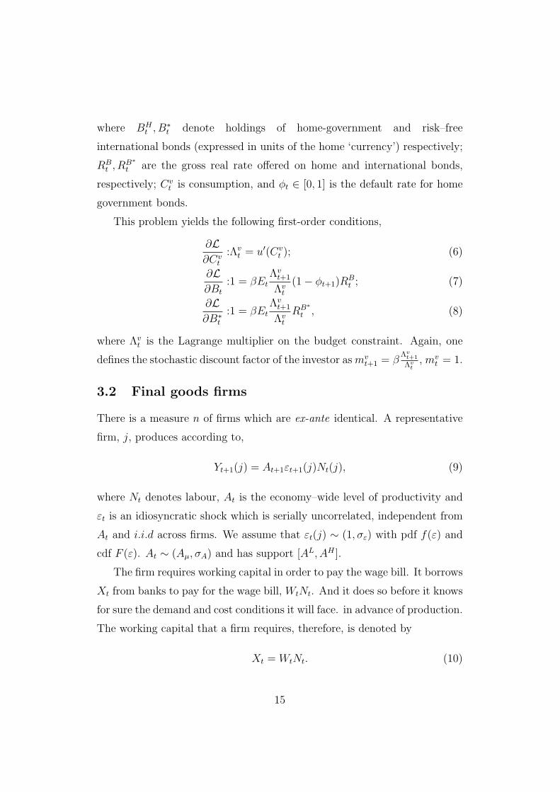
where BHt , B∗

t denote holdings of home-government and risk–free

international bonds (expressed in units of the home ‘currency’) respectively;

RBt , R

B∗t are the gross real rate offered on home and international bonds,

respectively; Cvt is consumption, and ϕt ∈ [0, 1] is the default rate for home

government bonds.

This problem yields the following first-order conditions,

∂L∂Cv

t

:Λvt = u′(Cv

t ); (6)

∂L∂Bt

:1 = βEt

Λvt+1

Λvt

(1− ϕt+1)RBt ; (7)

∂L∂B∗

t

:1 = βEt

Λvt+1

Λvt

RB∗

t , (8)

where Λvt is the Lagrange multiplier on the budget constraint. Again, one

defines the stochastic discount factor of the investor asmvt+1 = β

Λvt+1

Λvt,mv

t = 1.

3.2 Final goods firms

There is a measure n of firms which are ex-ante identical. A representative

firm, j, produces according to,

Yt+1(j) = At+1εt+1(j)Nt(j), (9)

where Nt denotes labour, At is the economy–wide level of productivity and

εt is an idiosyncratic shock which is serially uncorrelated, independent from

At and i.i.d across firms. We assume that εt(j) ∼ (1, σε) with pdf f(ε) and

cdf F (ε). At ∼ (Aµ, σA) and has support [AL, AH ].

The firm requires working capital in order to pay the wage bill. It borrows

Xt from banks to pay for the wage bill, WtNt. And it does so before it knows

for sure the demand and cost conditions it will face. in advance of production.

The working capital that a firm requires, therefore, is denoted by

Xt = WtNt. (10)

15

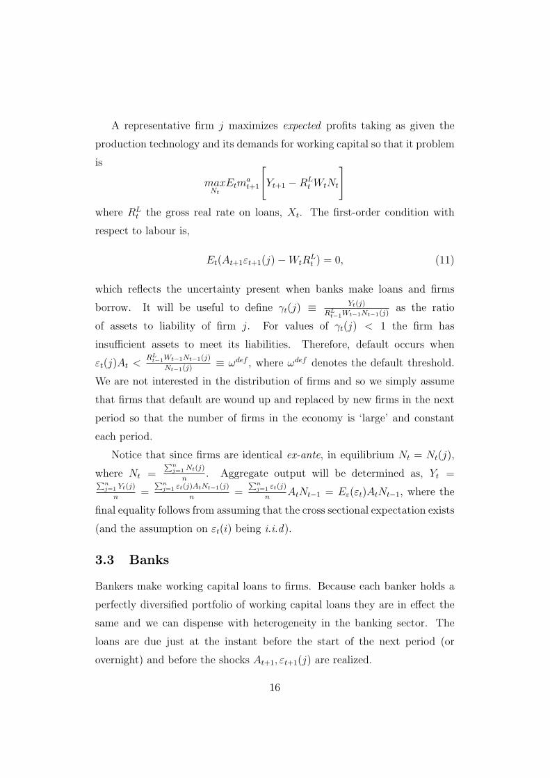
A representative firm j maximizes expected profits taking as given the

production technology and its demands for working capital so that it problem

is

maxNt

Etmat+1

[Yt+1 −RL

t WtNt

]where RL

t the gross real rate on loans, Xt. The first-order condition with

respect to labour is,

Et(At+1εt+1(j)−WtRLt ) = 0, (11)

which reflects the uncertainty present when banks make loans and firms

borrow. It will be useful to define γt(j) ≡ Yt(j)

RLt−1Wt−1Nt−1(j)

as the ratio

of assets to liability of firm j. For values of γt(j) < 1 the firm has

insufficient assets to meet its liabilities. Therefore, default occurs when

εt(j)At <RL

t−1Wt−1Nt−1(j)

Nt−1(j)≡ ωdef , where ωdef denotes the default threshold.

We are not interested in the distribution of firms and so we simply assume

that firms that default are wound up and replaced by new firms in the next

period so that the number of firms in the economy is ‘large’ and constant

each period.

Notice that since firms are identical ex-ante, in equilibrium Nt = Nt(j),

where Nt =∑n

j=1 Nt(j)

n. Aggregate output will be determined as, Yt =∑n

j=1 Yt(j)

n=

∑nj=1 εt(j)AtNt−1(j)

n=

∑nj=1 εt(j)

nAtNt−1 = Eε(εt)AtNt−1, where the

final equality follows from assuming that the cross sectional expectation exists

(and the assumption on εt(i) being i.i.d).

3.3 Banks

Bankers make working capital loans to firms. Because each banker holds a

perfectly diversified portfolio of working capital loans they are in effect the

same and we can dispense with heterogeneity in the banking sector. The

loans are due just at the instant before the start of the next period (or

overnight) and before the shocks At+1, εt+1(j) are realized.

16

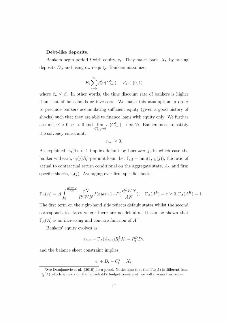
Debt-like deposits.

Bankers begin period t with equity, et. They make loans, Xt, by raising

deposits Dt, and using own equity. Bankers maximize,

Et

∞∑i=0

βibυ(C

bt+i), βb ∈ (0, 1)

where βb ≤ β. In other words, the time discount rate of bankers is higher

than that of households or investors. We make this assumption in order

to preclude bankers accumulating sufficient equity (given a good history of

shocks) such that they are able to finance loans with equity only. We further

assume, υ′ > 0, υ′′ < 0 and limCb

t+i→0υ′(Cb

t+i) → ∞,∀i. Bankers need to satisfy

the solvency constraint,

et+i ≥ 0.

As explained, γt(j) < 1 implies default by borrower j, in which case the

banker will earn, γt(j)RLt per unit loan. Let ΓεA = min(1, γt(j)), the ratio of

actual to contractual return conditional on the aggregate state, At, and firm

specific shocks, εt(j). Averaging over firm-specific shocks,

ΓA(A) = A

∫ RLWNAN

0

εN

RLWNf(ε)dε+1−F (

RLWN

AN), ΓA(A

L) = ς ≥ 0,ΓA(AH) = 1

The first term on the right-hand side reflects default states whilst the second

corresponds to states where there are no defaults. It can be shown that

ΓA(A) is an increasing and concave function of A.9

Bankers’ equity evolves as,

et+1 = ΓA(At+1)RLt Xt −RD

t Dt,

and the balance sheet constraint implies,

et +Dt − Cbt = Xt,

9See Damjanovic et al. (2016) for a proof. Notice also that this ΓA(A) is different fromΓsA(A) which appears on the household’s budget constraint, we will discuss this below.

17

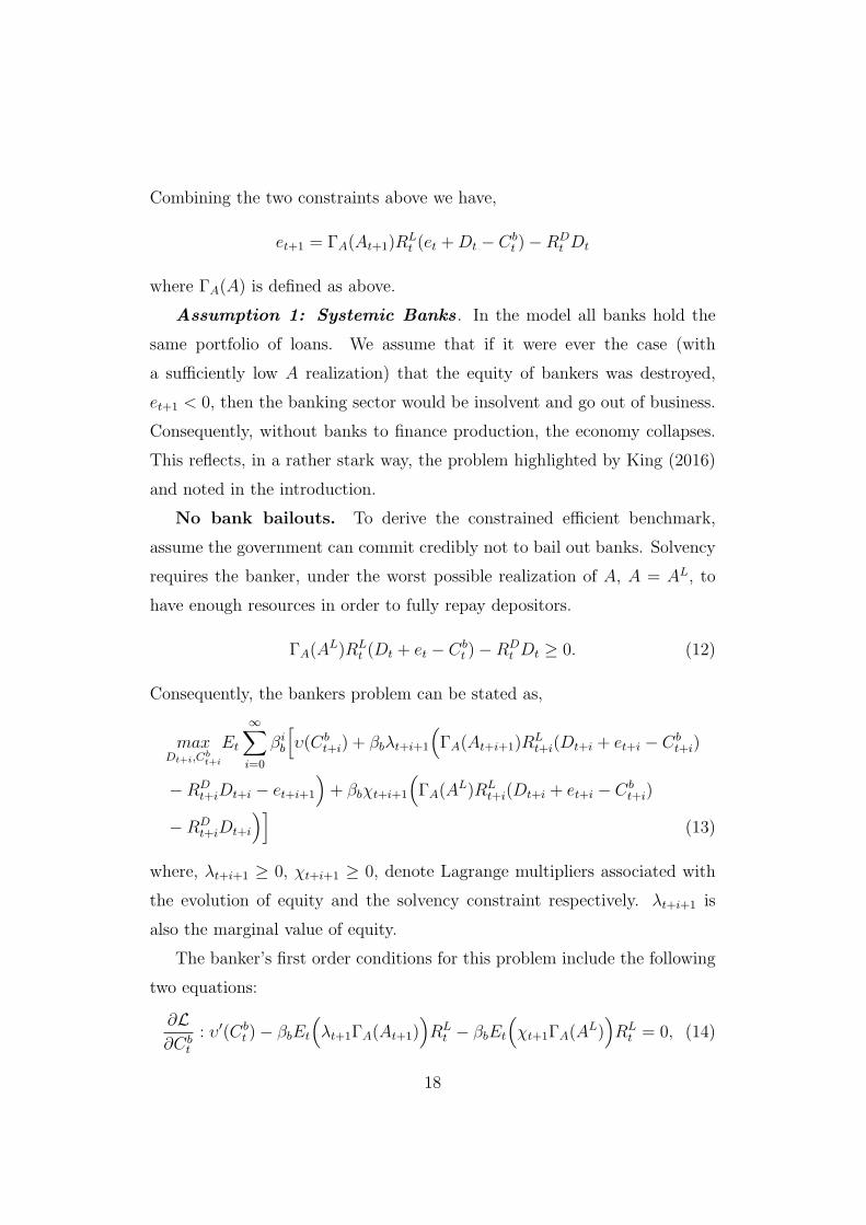
Combining the two constraints above we have,

et+1 = ΓA(At+1)RLt (et +Dt − Cb

t )−RDt Dt

where ΓA(A) is defined as above.

Assumption 1: Systemic Banks . In the model all banks hold the

same portfolio of loans. We assume that if it were ever the case (with

a sufficiently low A realization) that the equity of bankers was destroyed,

et+1 < 0, then the banking sector would be insolvent and go out of business.

Consequently, without banks to finance production, the economy collapses.

This reflects, in a rather stark way, the problem highlighted by King (2016)

and noted in the introduction.

No bank bailouts. To derive the constrained efficient benchmark,

assume the government can commit credibly not to bail out banks. Solvency

requires the banker, under the worst possible realization of A, A = AL, to

have enough resources in order to fully repay depositors.

ΓA(AL)RL

t (Dt + et − Cbt )−RD

t Dt ≥ 0. (12)

Consequently, the bankers problem can be stated as,

maxDt+i,Cb

t+i

Et

∞∑i=0

βib

[υ(Cb

t+i) + βbλt+i+1

(ΓA(At+i+1)R

Lt+i(Dt+i + et+i − Cb

t+i)

−RDt+iDt+i − et+i+1

)+ βbχt+i+1

(ΓA(A

L)RLt+i(Dt+i + et+i − Cb

t+i)

−RDt+iDt+i

)](13)

where, λt+i+1 ≥ 0, χt+i+1 ≥ 0, denote Lagrange multipliers associated with

the evolution of equity and the solvency constraint respectively. λt+i+1 is

also the marginal value of equity.

The banker’s first order conditions for this problem include the following

two equations:

∂L∂Cb

t

: υ′(Cbt )− βbEt

(λt+1ΓA(At+1)

)RL

t − βbEt

(χt+1ΓA(A

L))RL

t = 0, (14)

18

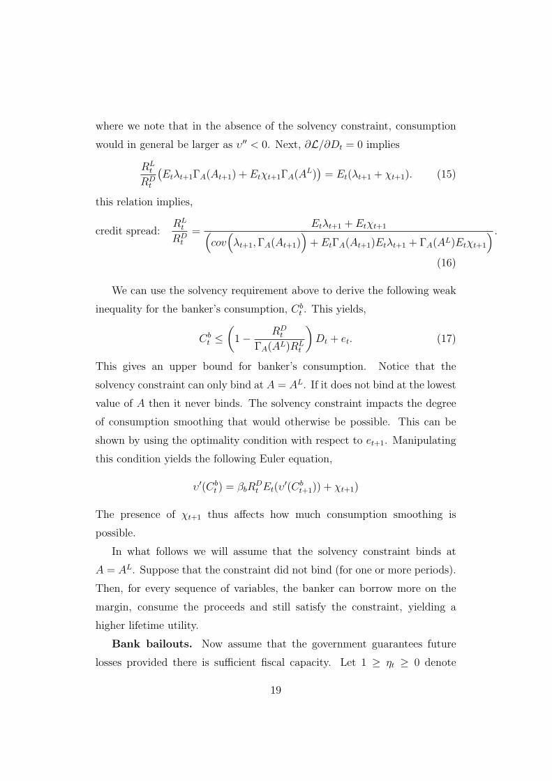
where we note that in the absence of the solvency constraint, consumption

would in general be larger as υ′′ < 0. Next, ∂L/∂Dt = 0 implies

RLt

RDt

(Etλt+1ΓA(At+1) + Etχt+1ΓA(A

L))= Et(λt+1 + χt+1). (15)

this relation implies,

credit spread:RL

t

RDt

=Etλt+1 + Etχt+1(

cov(λt+1,ΓA(At+1)

)+ EtΓA(At+1)Etλt+1 + ΓA(AL)Etχt+1

) .(16)

We can use the solvency requirement above to derive the following weak

inequality for the banker’s consumption, Cbt . This yields,

Cbt ≤

(1− RD

t

ΓA(AL)RLt

)Dt + et. (17)

This gives an upper bound for banker’s consumption. Notice that the

solvency constraint can only bind at A = AL. If it does not bind at the lowest

value of A then it never binds. The solvency constraint impacts the degree

of consumption smoothing that would otherwise be possible. This can be

shown by using the optimality condition with respect to et+1. Manipulating

this condition yields the following Euler equation,

υ′(Cbt ) = βbR

Dt Et(υ

′(Cbt+1)) + χt+1)

The presence of χt+1 thus affects how much consumption smoothing is

possible.

In what follows we will assume that the solvency constraint binds at

A = AL. Suppose that the constraint did not bind (for one or more periods).

Then, for every sequence of variables, the banker can borrow more on the

margin, consume the proceeds and still satisfy the constraint, yielding a

higher lifetime utility.

Bank bailouts. Now assume that the government guarantees future

losses provided there is sufficient fiscal capacity. Let 1 ≥ ηt ≥ 0 denote

19

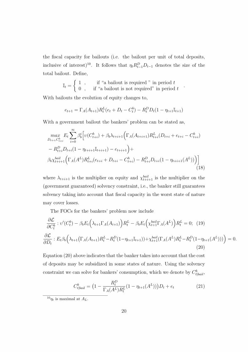
the fiscal capacity for bailouts (i.e. the bailout per unit of total deposits,

inclusive of interest)10. It follows that ηtRDt−1Dt−1 denotes the size of the

total bailout. Define,

It ={

1 ,0 ,

if “a bailout is required ” in period tif “a bailout is not required” in period t

.

With bailouts the evolution of equity changes to,

et+1 = ΓA(At+1)RLt (et +Dt − Cb

t )−RDt Dt(1− ηt+1It+1)

With a government bailout the bankers’ problem can be stated as,

maxDt+i,Cb

t+i

Et

∞∑i=0

βib

[υ(Cb

t+i) + βbλt+i+1

(ΓA(At+i+1)R

Lt+i(Dt+i + et+i − Cb

t+i)

−RDt+iDt+i(1− ηt+i+1It+i+1)− et+i+1

)+

βbχbailt+i+1

(ΓA(A

L)RLt+i(et+i +Dt+i − Cb

t+i)−RDt+iDt+i(1− ηt+i+1(A

L)))](18)

where λt+i+1 is the multiplier on equity and χbailt+i+1 is the multiplier on the

(government guaranteed) solvency constraint, i.e., the banker still guarantees

solvency taking into account that fiscal capacity in the worst state of nature

may cover losses.

The FOCs for the bankers’ problem now include

∂L∂Cb

t

: υ′(Cbt )− βbEt

(λt+1ΓA(At+1)

)RL

t − βbEt

(χbailt+1ΓA(A

L))RL

t = 0; (19)

∂L∂Dt

: Etβb

(λt+1

(ΓA(At+1)R

Lt −RD

t (1−ηt+1It+1))+χbailt+1(ΓA(A

L)RLt −RD

t (1−ηt+1(AL)))

)= 0.

(20)

Equation (20) above indicates that the banker takes into account that the cost

of deposits may be subsidized in some states of nature. Using the solvency

constraint we can solve for bankers’ consumption, which we denote by Cbt|bail,

Cbt|bail =

(1− RD

t

ΓA(AL)RLt

(1− ηt+1(AL))

)Dt + et (21)

10ηt is maximal at AL.

20

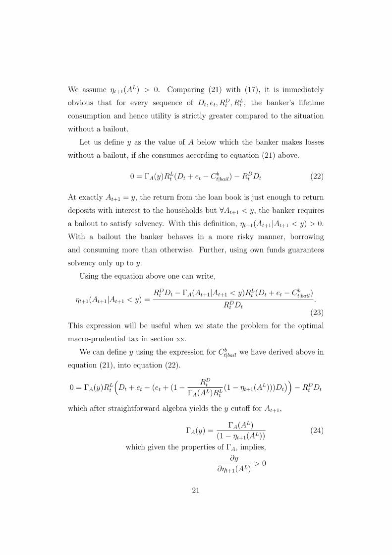
We assume ηt+1(AL) > 0. Comparing (21) with (17), it is immediately

obvious that for every sequence of Dt, et, RDt , R

Lt , the banker’s lifetime

consumption and hence utility is strictly greater compared to the situation

without a bailout.

Let us define y as the value of A below which the banker makes losses

without a bailout, if she consumes according to equation (21) above.

0 = ΓA(y)RLt (Dt + et − Cb

t|bail)−RDt Dt (22)

At exactly At+1 = y, the return from the loan book is just enough to return

deposits with interest to the households but ∀At+1 < y, the banker requires

a bailout to satisfy solvency. With this definition, ηt+1(At+1|At+1 < y) > 0.

With a bailout the banker behaves in a more risky manner, borrowing

and consuming more than otherwise. Further, using own funds guarantees

solvency only up to y.

Using the equation above one can write,

ηt+1(At+1|At+1 < y) =RD

t Dt − ΓA(At+1|At+1 < y)RLt (Dt + et − Cb

t|bail)

RDt Dt

.

(23)

This expression will be useful when we state the problem for the optimal

macro-prudential tax in section xx.

We can define y using the expression for Cbt|bail we have derived above in

equation (21), into equation (22).

0 = ΓA(y)RLt

(Dt + et − (et + (1− RD

t

ΓA(AL)RLt

(1− ηt+1(AL)))Dt

))−RD

t Dt

which after straightforward algebra yields the y cutoff for At+1,

ΓA(y) =ΓA(A

L)

(1− ηt+1(AL))(24)

which given the properties of ΓA, implies,

∂y

∂ηt+1(AL)> 0

21

In other words, if the banker expects higher fiscal capacity she behaves

more risky. The sign of the derivative is key for the design of the optimal

macroprudential tax.

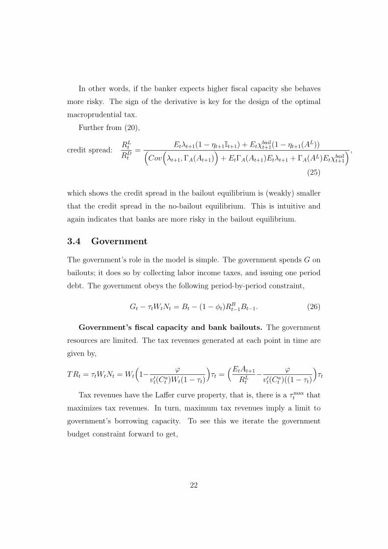
Further from (20),

credit spread:RL

t

RDt

=Etλt+1(1− ηt+1It+1) + Etχ

bailt+1(1− ηt+1(A

L))(Cov

(λt+1,ΓA(At+1)

)+ EtΓA(At+1)Etλt+1 + ΓA(AL)Etχbail

t+1

) ,(25)

which shows the credit spread in the bailout equilibrium is (weakly) smaller

that the credit spread in the no-bailout equilibrium. This is intuitive and

again indicates that banks are more risky in the bailout equilibrium.

3.4 Government

The government’s role in the model is simple. The government spends G on

bailouts; it does so by collecting labor income taxes, and issuing one period

debt. The government obeys the following period-by-period constraint,

Gt − τtWtNt = Bt − (1− ϕt)RBt−1Bt−1. (26)

Government’s fiscal capacity and bank bailouts. The government

resources are limited. The tax revenues generated at each point in time are

given by,

TRt = τtWtNt = Wt

(1− φ

v′t(Cat )Wt(1− τt)

)τt =

(EtAt+1

RLt

− φ

v′t(Cat )((1− τt)

)τt

Tax revenues have the Laffer curve property, that is, there is a τmaxt that

maximizes tax revenues. In turn, maximum tax revenues imply a limit to

government’s borrowing capacity. To see this we iterate the government

budget constraint forward to get,

22

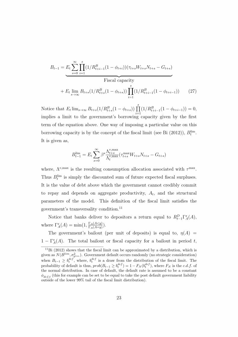
Bt−1 = Et

∞∑s=0

s∏i=1

(1/RBt+i−1(1− ϕt+i))(τt+sWt+sNt+s −Gt+s)︸ ︷︷ ︸

Fiscal capacity

+ Et lims→∞

Bt+s(1/RBt+s(1− ϕt+s))

s∏i=1

(1/RBt+i−1(1− ϕt+i−1)) (27)

Notice that Et lims→∞ Bt+s(1/RBt+s(1− ϕt+s))

s∏i=1

(1/RBt+i−1(1− ϕt+i−1)) = 0,

implies a limit to the government’s borrowing capacity given by the first

term of the equation above. One way of imposing a particular value on this

borrowing capacity is by the concept of the fiscal limit (see Bi (2012)), Blimt .

It is given as,

Blimt−1 = Et

∞∑s=0

βsΛv,maxt+s

Λv,maxt

(τmaxt+s Wt+sNt+s −Gt+s)

where, Λv,max is the resulting consumption allocation associated with τmax.

Thus Blimt is simply the discounted sum of future expected fiscal surpluses.

It is the value of debt above which the government cannot credibly commit

to repay and depends on aggregate productivity, At, and the structural

parameters of the model. This definition of the fiscal limit satisfies the

government’s transversality condition.11

Notice that banks deliver to depositors a return equal to RDt−1Γ

sA(A),

where ΓsA(A) = min(1, ΓA(A<y)

ΓA(A=y)).

The government’s bailout (per unit of deposits) is equal to, η(A) =

1 − ΓsA(A). The total bailout or fiscal capacity for a bailout in period t,

11Bi (2012) shows that the fiscal limit can be approximated by a distribution, which isgiven as N(Blim, σ2

blim). Government default occurs randomly (no strategic consideration)

when Bt−1 ≥ bdeft , where, bdeft is a draw from the distribution of the fiscal limit. The

probability of default is thus, prob(Bt−1 ≥ bdeft ) = 1−FN (bdeft ), where FN is the c.d.f. ofthe normal distribution. In case of default, the default rate is assumed to be a constantϕdef,t (this for example can be set to be equal to take the post default government liabilityoutside of the lower 99% tail of the fiscal limit distribution).

23

is given as,

Gt = min[ηt(At)Dt−1RDt−1, B

limt − (1− ϕt)R

Bt−1Bt−1 + τtWtNt] (28)

3.5 Market Clearing

Define total consumption,

Ct = Cat + Cb

t + Cvt (29)

Equilibrium in the final goods market,

Ct +Gt = Yt (30)

Equilibrium in the loan market,

Xt = Xst = Xd

t = WtNt (31)

where, Xst , X

dt denote loan supply and loan demand respectively.

Government bond market equilibrium,

Bt = BHt (32)

3.6 Time inconsistency of the no-bailout commitment

We begin with the following definition of equilibrium conditional on the

government being able to credibly commit to never bail-out the bankers.

Definition 1. The constrained efficient equilibrium corresponds to an

allocation where bankers never experience negative equity, distortive labor

taxes on private agents are time invariant and always as low as possible (or

never levied), deposits are safe, investors never experience haircuts and gov-

ernment debt is time invariant. Given the stochastic processes for At, εt+1(j),

24

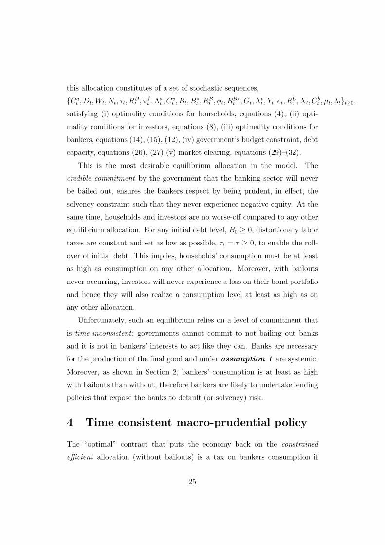
this allocation constitutes of a set of stochastic sequences,

{Cat , Dt,Wt, Nt, τt, R

Dt , π

ft ,Λ

at , C

vt , Bt, B

∗t , R

Bt , ϕt, R

B∗t , Gt,Λ

vt , Yt, et, R

Lt , Xt, C

bt , µt, λt}t≥0,

satisfying (i) optimality conditions for households, equations (4), (ii) opti-

mality conditions for investors, equations (8), (iii) optimality conditions for

bankers, equations (14), (15), (12), (iv) government’s budget constraint, debt

capacity, equations (26), (27) (v) market clearing, equations (29)–(32).

This is the most desirable equilibrium allocation in the model. The

credible commitment by the government that the banking sector will never

be bailed out, ensures the bankers respect by being prudent, in effect, the

solvency constraint such that they never experience negative equity. At the

same time, households and investors are no worse-off compared to any other

equilibrium allocation. For any initial debt level, B0 ≥ 0, distortionary labor

taxes are constant and set as low as possible, τt = τ ≥ 0, to enable the roll-

over of initial debt. This implies, households’ consumption must be at least

as high as consumption on any other allocation. Moreover, with bailouts

never occurring, investors will never experience a loss on their bond portfolio

and hence they will also realize a consumption level at least as high as on

any other allocation.

Unfortunately, such an equilibrium relies on a level of commitment that

is time-inconsistent ; governments cannot commit to not bailing out banks

and it is not in bankers’ interests to act like they can. Banks are necessary

for the production of the final good and under assumption 1 are systemic.

Moreover, as shown in Section 2, bankers’ consumption is at least as high

with bailouts than without, therefore bankers are likely to undertake lending

policies that expose the banks to default (or solvency) risk.

4 Time consistent macro-prudential policy

The “optimal” contract that puts the economy back on the constrained

efficient allocation (without bailouts) is a tax on bankers consumption if

25

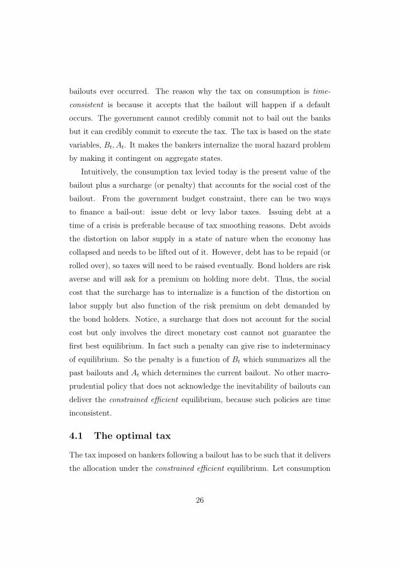
bailouts ever occurred. The reason why the tax on consumption is time-

consistent is because it accepts that the bailout will happen if a default

occurs. The government cannot credibly commit not to bail out the banks

but it can credibly commit to execute the tax. The tax is based on the state

variables, Bt, At. It makes the bankers internalize the moral hazard problem

by making it contingent on aggregate states.

Intuitively, the consumption tax levied today is the present value of the

bailout plus a surcharge (or penalty) that accounts for the social cost of the

bailout. From the government budget constraint, there can be two ways

to finance a bail-out: issue debt or levy labor taxes. Issuing debt at a

time of a crisis is preferable because of tax smoothing reasons. Debt avoids

the distortion on labor supply in a state of nature when the economy has

collapsed and needs to be lifted out of it. However, debt has to be repaid (or

rolled over), so taxes will need to be raised eventually. Bond holders are risk

averse and will ask for a premium on holding more debt. Thus, the social

cost that the surcharge has to internalize is a function of the distortion on

labor supply but also function of the risk premium on debt demanded by

the bond holders. Notice, a surcharge that does not account for the social

cost but only involves the direct monetary cost cannot not guarantee the

first best equilibrium. In fact such a penalty can give rise to indeterminacy

of equilibrium. So the penalty is a function of Bt which summarizes all the

past bailouts and At which determines the current bailout. No other macro-

prudential policy that does not acknowledge the inevitability of bailouts can

deliver the constrained efficient equilibrium, because such policies are time

inconsistent.

4.1 The optimal tax

The tax imposed on bankers following a bailout has to be such that it delivers

the allocation under the constrained efficient equilibrium. Let consumption

26

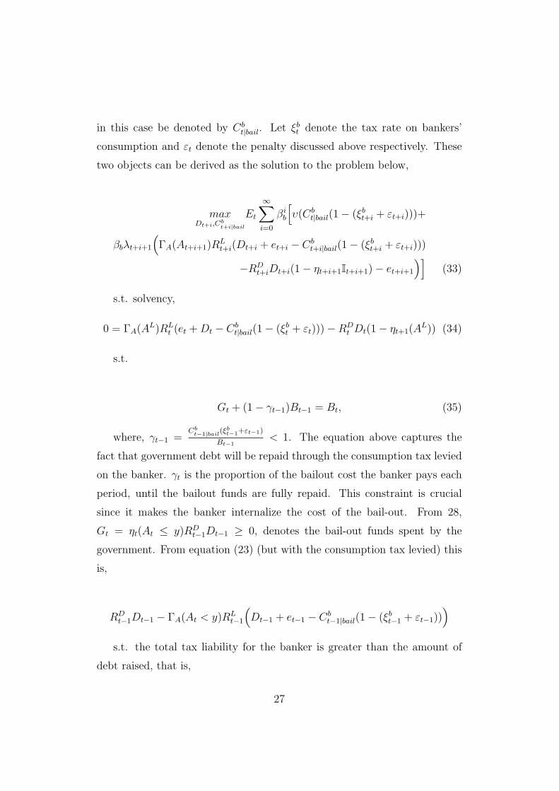
in this case be denoted by Cbt|bail. Let ξbt denote the tax rate on bankers’

consumption and εt denote the penalty discussed above respectively. These

two objects can be derived as the solution to the problem below,

maxDt+i,Cb

t+i|bail

Et

∞∑i=0

βib

[υ(Cb

t|bail(1− (ξbt+i + εt+i)))+

βbλt+i+1

(ΓA(At+i+1)R

Lt+i(Dt+i + et+i − Cb

t+i|bail(1− (ξbt+i + εt+i)))

−RDt+iDt+i(1− ηt+i+1It+i+1)− et+i+1

)](33)

s.t. solvency,

0 = ΓA(AL)RL

t (et +Dt − Cbt|bail(1− (ξbt + εt)))−RD

t Dt(1− ηt+1(AL)) (34)

s.t.

Gt + (1− γt−1)Bt−1 = Bt, (35)

where, γt−1 =Cb

t−1|bail(ξbt−1+εt−1)

Bt−1< 1. The equation above captures the

fact that government debt will be repaid through the consumption tax levied

on the banker. γt is the proportion of the bailout cost the banker pays each

period, until the bailout funds are fully repaid. This constraint is crucial

since it makes the banker internalize the cost of the bail-out. From 28,

Gt = ηt(At ≤ y)RDt−1Dt−1 ≥ 0, denotes the bail-out funds spent by the

government. From equation (23) (but with the consumption tax levied) this

is,

RDt−1Dt−1 − ΓA(At < y)RL

t−1

(Dt−1 + et−1 − Cb

t−1|bail(1− (ξbt−1 + εt−1)))

s.t. the total tax liability for the banker is greater than the amount of

debt raised, that is,

27

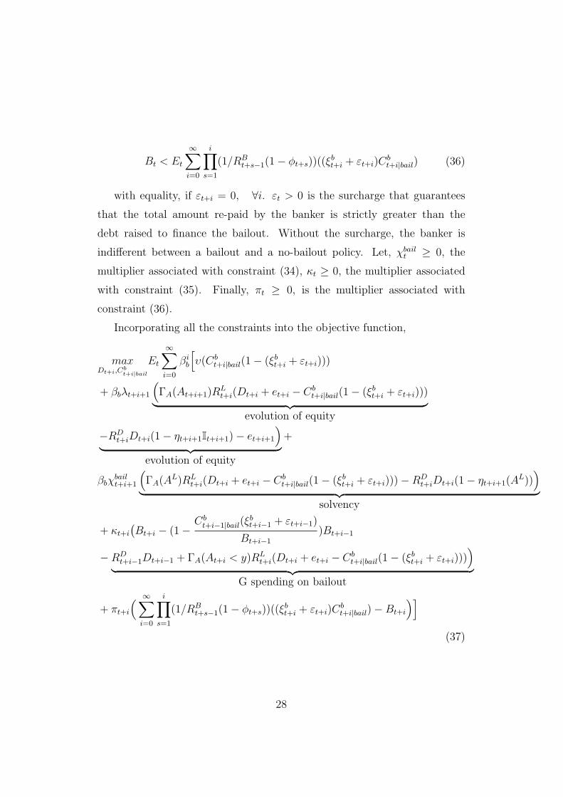
Bt < Et

∞∑i=0

i∏s=1

(1/RBt+s−1(1− ϕt+s))((ξ

bt+i + εt+i)C

bt+i|bail) (36)

with equality, if εt+i = 0, ∀i. εt > 0 is the surcharge that guarantees

that the total amount re-paid by the banker is strictly greater than the

debt raised to finance the bailout. Without the surcharge, the banker is

indifferent between a bailout and a no-bailout policy. Let, χbailt ≥ 0, the

multiplier associated with constraint (34), κt ≥ 0, the multiplier associated

with constraint (35). Finally, πt ≥ 0, is the multiplier associated with

constraint (36).

Incorporating all the constraints into the objective function,

maxDt+i,Cb

t+i|bail

Et

∞∑i=0

βib

[υ(Cb

t+i|bail(1− (ξbt+i + εt+i)))

+ βbλt+i+1

(ΓA(At+i+1)R

Lt+i(Dt+i + et+i − Cb

t+i|bail(1− (ξbt+i + εt+i)))︸ ︷︷ ︸evolution of equity

−RDt+iDt+i(1− ηt+i+1It+i+1)− et+i+1

)︸ ︷︷ ︸

evolution of equity

+

βbχbailt+i+1

(ΓA(A

L)RLt+i(Dt+i + et+i − Cb

t+i|bail(1− (ξbt+i + εt+i)))−RDt+iDt+i(1− ηt+i+1(A

L)))

︸ ︷︷ ︸solvency

+ κt+i

(Bt+i − (1−

Cbt+i−1|bail(ξ

bt+i−1 + εt+i−1)

Bt+i−1

)Bt+i−1

−RDt+i−1Dt+i−1 + ΓA(At+i < y)RL

t+i(Dt+i + et+i − Cbt+i|bail(1− (ξbt+i + εt+i)))

)︸ ︷︷ ︸

G spending on bailout

+ πt+i

( ∞∑i=0

i∏s=1

(1/RBt+s−1(1− ϕt+s))((ξ

bt+i + εt+i)C

bt+i|bail)−Bt+i

)](37)

28

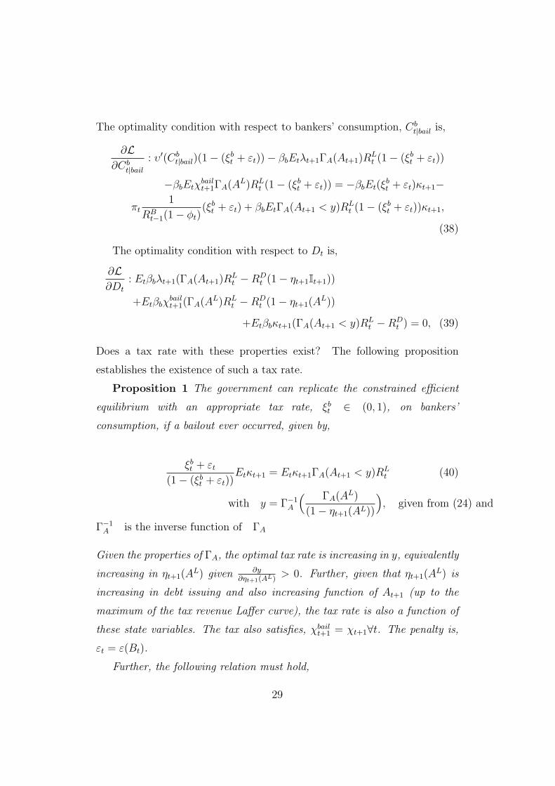
The optimality condition with respect to bankers’ consumption, Cbt|bail is,

∂L∂Cb

t|bail: υ′(Cb

t|bail)(1− (ξbt + εt))− βbEtλt+1ΓA(At+1)RLt (1− (ξbt + εt))

−βbEtχbailt+1ΓA(A

L)RLt (1− (ξbt + εt)) = −βbEt(ξ

bt + εt)κt+1−

πt1

RBt−1(1− ϕt)

(ξbt + εt) + βbEtΓA(At+1 < y)RLt (1− (ξbt + εt))κt+1,

(38)

The optimality condition with respect to Dt is,

∂L∂Dt

: Etβbλt+1(ΓA(At+1)RLt −RD

t (1− ηt+1It+1))

+Etβbχbailt+1(ΓA(A

L)RLt −RD

t (1− ηt+1(AL))

+Etβbκt+1(ΓA(At+1 < y)RLt −RD

t ) = 0, (39)

Does a tax rate with these properties exist? The following proposition

establishes the existence of such a tax rate.

Proposition 1 The government can replicate the constrained efficient

equilibrium with an appropriate tax rate, ξbt ∈ (0, 1), on bankers’

consumption, if a bailout ever occurred, given by,

ξbt + εt(1− (ξbt + εt))

Etκt+1 = Etκt+1ΓA(At+1 < y)RLt (40)

with y = Γ−1A

( ΓA(AL)

(1− ηt+1(AL))

), given from (24) and

Γ−1A is the inverse function of ΓA

Given the properties of ΓA, the optimal tax rate is increasing in y, equivalently

increasing in ηt+1(AL) given ∂y

∂ηt+1(AL)> 0. Further, given that ηt+1(A

L) is

increasing in debt issuing and also increasing function of At+1 (up to the

maximum of the tax revenue Laffer curve), the tax rate is also a function of

these state variables. The tax also satisfies, χbailt+1 = χt+1∀t. The penalty is,

εt = ε(Bt).

Further, the following relation must hold,

29

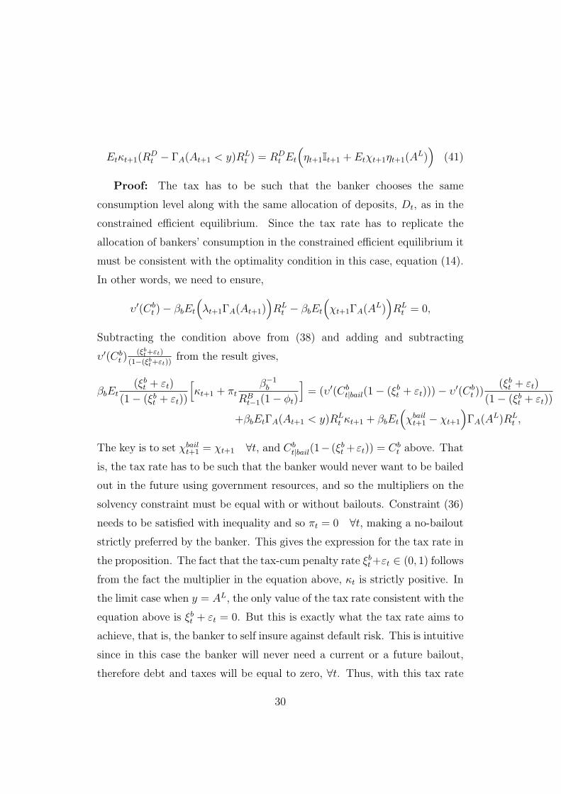
Etκt+1(RDt − ΓA(At+1 < y)RL

t ) = RDt Et

(ηt+1It+1 + Etχt+1ηt+1(A

L))

(41)

Proof: The tax has to be such that the banker chooses the same

consumption level along with the same allocation of deposits, Dt, as in the

constrained efficient equilibrium. Since the tax rate has to replicate the

allocation of bankers’ consumption in the constrained efficient equilibrium it

must be consistent with the optimality condition in this case, equation (14).

In other words, we need to ensure,

υ′(Cbt )− βbEt

(λt+1ΓA(At+1)

)RL

t − βbEt

(χt+1ΓA(A

L))RL

t = 0,

Subtracting the condition above from (38) and adding and subtracting

υ′(Cbt )

(ξbt+εt)

(1−(ξbt+εt))from the result gives,

βbEt(ξbt + εt)

(1− (ξbt + εt))

[κt+1 + πt

β−1b

RBt−1(1− ϕt)

]= (υ′(Cb

t|bail(1− (ξbt + εt)))− υ′(Cbt ))

(ξbt + εt)

(1− (ξbt + εt))

+βbEtΓA(At+1 < y)RLt κt+1 + βbEt

(χbailt+1 − χt+1

)ΓA(A

L)RLt ,

The key is to set χbailt+1 = χt+1 ∀t, and Cb

t|bail(1− (ξbt +εt)) = Cbt above. That

is, the tax rate has to be such that the banker would never want to be bailed

out in the future using government resources, and so the multipliers on the

solvency constraint must be equal with or without bailouts. Constraint (36)

needs to be satisfied with inequality and so πt = 0 ∀t, making a no-bailout

strictly preferred by the banker. This gives the expression for the tax rate in

the proposition. The fact that the tax-cum penalty rate ξbt+εt ∈ (0, 1) follows

from the fact the multiplier in the equation above, κt is strictly positive. In

the limit case when y = AL, the only value of the tax rate consistent with the

equation above is ξbt + εt = 0. But this is exactly what the tax rate aims to

achieve, that is, the banker to self insure against default risk. This is intuitive

since in this case the banker will never need a current or a future bailout,

therefore debt and taxes will be equal to zero, ∀t. Thus, with this tax rate

30

in place, bailouts will never occur, distortive labor taxes will never be levied

and government debt will be equal to zero. Given the only inefficiency in

the model is the moral hazard taken by the bankers’, a tax that eliminates

it, satisfies the optimality conditions of the other agents in the economy

and delivers the constrained efficient equilibrium. The penalty surcharge is

a function of debt. A bailout can be financed in three ways, (i) issuing new

debt, (ii) labor taxes, (iii) losses to bondholders. Any of the three imply

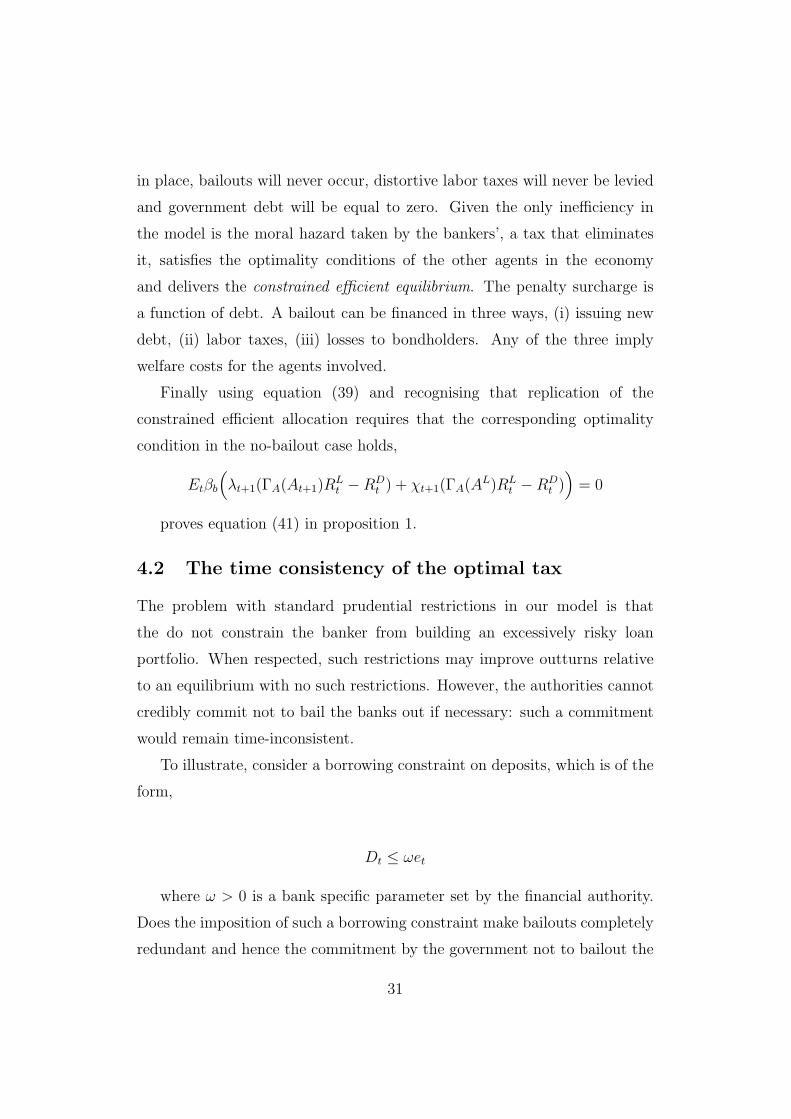
welfare costs for the agents involved.

Finally using equation (39) and recognising that replication of the

constrained efficient allocation requires that the corresponding optimality

condition in the no-bailout case holds,

Etβb

(λt+1(ΓA(At+1)R

Lt −RD

t ) + χt+1(ΓA(AL)RL

t −RDt )

)= 0

proves equation (41) in proposition 1.

4.2 The time consistency of the optimal tax

The problem with standard prudential restrictions in our model is that

the do not constrain the banker from building an excessively risky loan

portfolio. When respected, such restrictions may improve outturns relative

to an equilibrium with no such restrictions. However, the authorities cannot

credibly commit not to bail the banks out if necessary: such a commitment

would remain time-inconsistent.

To illustrate, consider a borrowing constraint on deposits, which is of the

form,

Dt ≤ ωet

where ω > 0 is a bank specific parameter set by the financial authority.

Does the imposition of such a borrowing constraint make bailouts completely

redundant and hence the commitment by the government not to bailout the

31

bankers time consistent? In other words, is it in the bankers interests to

self insure against solvency risk and never require a bailout? We claim

that bailouts will still occur under this policy and the reason is simple.

The banker still has the option to consume more and hence achieve higher

utility compared to the constrained efficient allocation, if it expects that the

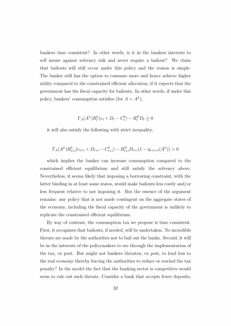
government has the fiscal capacity for bailouts. In other words, if under this

policy, bankers’ consumption satisfies (for A = AL),

ΓA(AL)RL

t (et +Dt − Cbt )−RD

t Dt ≥ 0

it will also satisfy the following with strict inequality,

ΓA(AL)RL

t+i(et+i +Dt+i − Cbt+i)−RD

t+iDt+i(1− ηt+i+1(AL)) > 0

which implies the banker can increase consumption compared to the

constrained efficient equilibrium and still satisfy the solvency above.

Nevertheless, it seems likely that imposing a borrowing constraint, with the

latter binding in at least some states, would make bailouts less costly and/or

less frequent relative to not imposing it. But the essence of the argument

remains: any policy that is not made contingent on the aggregate states of

the economy, including the fiscal capacity of the government is unlikely to

replicate the constrained efficient equilibrium.

By way of contrast, the consumption tax we propose is time consistent.

First, it recognises that bailouts, if needed, will be undertaken. No incredible

threats are made by the authorities not to bail out the banks. Second, it will

be in the interests of the policymakers to see through the implementation of

the tax, ex post. But might not bankers threaten, ex post, to lend less to

the real economy thereby forcing the authorities to reduce or rescind the tax

penalty? In the model the fact that the banking sector is competitive would

seem to rule out such threats. Consider a bank that accepts fewer deposits,

32

makes fewer loans and accepts lower consumption by way of executing this

threat. Or perhaps, raises more deposits than it lends out investing the rest

in less risky, lower-yielding assets. Competition means the cost of raising

deposits is taken as given. If the authorities impose the tax nonetheless,

then the bankers consumption will be lower than it otherwise could have

been, in either scenario, had he or she accepted more deposits and made

more loans. The bankers threats lack credibility. It is in the governments

interest to levy the tax and the bankers interest to pay the tax and optimize

of profitable lending opportunities.

5 How might the penalty work?

This paper has argued that a way to avoid bailouts is credibly to propose

penalties on bankers’ consumption. A number of obvious practical questions

spring to mind. On which individuals and institutions should such penalties

be levied? Would such penalties be time consistent and/or politically

feasible? Are such penalties ’fair’? What form might these penalties take?

On whom should penalties fall? Following most bailouts, shareholders are

typically ’wiped out’. Perhaps it may be possible to penalise shareholders

further in order to encourage closer monitoring of bank senior management.

However, we envisage the penalties proposed here as falling on key individuals

in designated systemically important financial institutions. That would

go with the grain of some recent supervisory developments. For example,

in some supervisory regimes certain regulated institutions already have to

identify key individuals. In addition, the Financial Stability Board designates

systemically important financial institutions. And supervisory agencies in

many countries increasingly take a view on which institutions they regards

as of national systemic importance and which roles and named individuals

are key. Such a regime as suggested in this paper could clearly go wider than

just banking firms and, along with higher capital requirements and other

33

prudential measures, would further discourage institutions from growing too

large. So, the penalties proposed here on key individuals in systemically

important financial institutions need not be levied on key individuals at all

institutions that are bailed out. Smaller institutions might not face such

penalties. If that turned out to lead to gaming of the system then the scope

of the penalties could be widened.

Are such penalties implementable? Calomiris and Haber (2014) argue

that many of the challenges society faces from the financial sector reflect

political preferences; banks, they argue, are ”fragile by design”. Another way

to put that, is that financial regulation is feeble by design. Why might the

penalties we propose be more robust than other regulatory measures? First,

these penalties should be transparent and their form agreed ex ante. Second,

following a bailout it would appear less costly, and perhaps even beneficial, to

politicians to see through the levying of these penalties. Acknowledging this,

banks/bankers should modify their behaviour ex ante. Even if bailouts were

necessary to restore confidence and maintain macroeconomic and financial

stability, penalties can be levied on individuals without exacerbating systemic

risk. This is in contrast to some new regulations such as new resolution

procedures. These procedures are agreed ex ante with a view to facilitating

the break-up of systemically important institutions that get in to trouble.

However, there are two problems in applying them. First, it is not clear how

far they alleviate excessive risk-taking ex ante. Second, resolution authorities

may still opt to recommend bailouts if resolution endangers wider financial

stability. The penalties we propose entail no such systemic risk.

What if a shock occurred that most thought impossible to anticipate?

Would levying penalties, following a bailout, in that case be ’unfair’ and

perhaps therefore unenforceable? Few anticipated the recent financial crisis

and its persistent impact on many economies. However, it is arguably the case

that few, especially inside banks, had sufficient incentive to monitor excessive

risk build up and fewer still to do anything about it. Moreover, recent work

34

by Schularick and Taylor (2012), Jorda et al. (2014) and others suggest

that ’credit booms gone bust’ have something of a predictable component

to them and so one may argue that with the right incentives many, perhaps

most, systemic crises are predictable. Nevertheless, what of the unforeseeable

event, the realisation of ’radical uncertainty’ as emphasized by King (2016)?

Even in this case the rationale for bailouts followed by penalties seems firmly

grounded. The designation of any institution as systemically important is

not contingent on the nature of the shock precipitating the crisis.

Finally, what form might penalties take? The penalties we envisage

should be levied on individuals. These individuals should be senior managers

who are key to deciding the risk profile of the bank or financial firm. Since

politicians will have an incentive to apply the penalties, bankers will have an

incentive to anticipate them in their decision-making. These penalties could

take a number of forms. They could be substantial financial fines enforced

by the courts. Or, they could be deductions to pension rights. They could be

delayed salary payments. Clearly, many details would need to be worked out.

But penalties should be made contingent on bailouts and strictly speaking

they should also be contingent on fiscal conditions although that may be

much harder still to calibrate and enforce.

6 Conclusions

In this paper we have argued that banks and other firms which are bailed out

should suffer a penalty contingent on that bailout. In the model, identifying

who should pay the penalty and calculating the size of that penalty

appear relatively simple. In practice no doubt things are more complex.

However, the regulatory authorities have made moves in the direction of the

arguments proposed in this paper. First, international bodies such as the

Financial Stability Board and the Basel Committee on Banking Supervision

have identified systemically important institutions. These institutions are

35

supervised more closely than other institutions and subject to stricter capital

and liquidity rules; the riskier their balance sheets are perceived to be, the

tighter the rules. In addition, other jurisdictions have introduced rules

on bonus claw-backs and closer oversight of individuals appointed to key

roles in large financial institutions. And many jurisdictions appear to be

moving towards stricter legal penalties for malfeasance. However, these

developments are all unrelated to what we argue is the central problem

in financial regulation; that is, governments cannot commit not to provide

periodic bailout. These rules discourage banks and other firms, at the margin,

from becoming bigger and riskier but do not incentivize these institutions

to become non-systemic and so the central dilemma in financial regulation

remains. Our argument works, we would assert, with the grain of the reforms

just mentioned but moves their focus to the central dilemma; our proposal

also focuses on key people in systemic institutions. The real-world analogue

of the consumption tax levied on bankers in this paper would need much

careful consideration. However, it may be take the form of a loss in pension

rights for those in charge of institutions that needed to be bailed out. It may

take the form of restrictions on bank shareholders. Or, some combination of

both.

References

Basu, K. and Dixit, A. (2014). Too small to regulate. Working Paper Series

6860, The World banks.

Bernanke, B. S., Gertler, M., and Gilchrist, S. (1999). The financial

accelerator in a quantitative business cycle framework. volume 1 of

Handbook of Macroeconomics, chapter 21, pages 1341–1393. Elsevier.

Bi, H. (2012). Sovereign default risk premia, fiscal limits, and fiscal policy.

European Economic Review, 56(3):389–410.

36

Bianchi, J. (2012). Efficient bailouts? NBER Working Papers 18587,

National Bureau of Economic Research, Inc.

Calomiris, C. and Haber, S. (2014). Fragile by design: The political origins

of banking crises and scarce credit. Princeton University Press.

Chari, V. and Phelan, C. (2014). Too correlated to fail. Economic Policy

Papers 14-3, Federal Reserve Bank of Minneapolis.

Correia, I., Farhi, E., Nicolini, J. P., and Teles, P. (2013). Unconventional

fiscal policy at the zero bound. American Economic Review, 103:1172–

1211.

Cunliffe, J. (2014). Ending too big to fail - progress to date and remaining

issues. Technical report, Speech given at the Barclays European Bank

Capital Summit, London.

Damjanovic, T., Damjanovic, V., and Nolan, C. (2013). Universal vs

separated banking with deposit insurance in a macro model. Technical

report.

Duncan, A. (2015). Monetary policy and herding. Mimeo.

Duncan, A. and Nolan, C. (2015). Objections and challenges of

macroprudential policy. Mimeo.

Farhi, E. and Tirole, J. (2012). Collective moral hazard, maturity mismatch,

and systemic bailouts. American Economic Review, 102:60–93.

Farhi, E. and Werning, I. (2013). A theory of macroprudential policies in

the presence of nominal rigidities. NBER Working Papers 19313, National

Bureau of Economic Research, Inc.

Friedman, M. and Schwartz, A. (1963). A monetary history of the united

states, 1867–1960. volume 3. National Bureau of Economic Research, Inc.,

1 edition.

37

Fund, I. M. (2014). Global financial stability report–moving from liquidity-

to growth-driven markets. Global Financial Stability Report, chapter 3.

IMF.

Gandhi, P. and Lustig, H. (2015). Size anomalies in u.s. bank stock returns.

Journal of Finance, 70:733–768.

Haldane, A. (2012). On being the right size. Speech given at Institute of

Economic Affairs 22nd Annual Series, The 2012 Beesley Lectures at the

Institute of Directors, Pall Mall, London.

Jeanne, O. and Korinek, A. (2010). Managing credit booms and busts: A

pigouvian taxation approach. NBER Working Papers 16377, National

Bureau of Economic Research, Inc.

Jeanne, O. and Korinek, A. (2014). Macroprudential policy beyond banking

regulation. Financial Stability Review, 18:163–172.

Jorda, O., Schularick, M., and Taylor, A. (2014). Sovereign versus banks:

Credit, crises and consequences. Federal Reserve Bank of San Francisco

Working paper, (2013-37).

Kelly, B., Lustig, H., and Nieuwerburgh, S. V. (2016). Too-systemic-to-

fail: What option markets imply about sector-wide government guarantees.

American Economic Review, xx:forthcoming.

King, M. (2016). The end of alchemy: Money, banking and the future of the

global economy. W.W. Norton and Company Inc.

Kiyotaki, N. and Moore, J. (1997). Credit cycles. Journal of Political

Economy, 105(2):211–48.

Laeven, L. and Valencia, F. (2013). Systemic banking crises database. IMF

Economic Review, 61:225–270.

38

Maurer, H. and Grussenmeyer, P. (2015). Financial assistance measures in

the euro area from 2008 to 2013: statistical framework and fiscal impact.

ECB Statistics Paper 7, European Central Bank.

Mendoza, E. and Bianchi, J. (2010). Overborrowing, financial crises and

macro prudential taxes. NBER Working Papers 16091, National Bureau

of Economic Research, Inc.

Mendoza, E. and Bianchi, J. (2013). Optimal time consistent

macroprudential policy. NBER Working Papers 19704, National Bureau

of Economic Research, Inc.

Mendoza, E. and Bianchi, J. (2015). Phases of global liquidity, fundamentals

news, and the design of macroprudential policy. BIS Working Papers 505,

BIS.

OHara, M. and Shaw, W. (1990). Deposit insurance and wealth effects: The

value of being too big to fail. Journal of Finance, 45:15871600.

Schmitt-Grohe, S. and Uribe, M. (2012). Prudential policy for peggers.

NBER Working Papers 18031, National Bureau of Economic Research,

Inc.

Schularick, M. and Taylor, A. (2012). Credit booms gone bust: Monetary

policy, leverage cycles and financial crises, 1870-2008. American Economic

Review, 102(2):1029–61.

39