Wireless Sensor Networks - uni-freiburg.de

1

University of FreiburgComputer Networks and Telematics

Prof. Christian Schindelhauer

Wireless SensorNetworks

4th Lecture07.11.2006

Christian [email protected]

University of FreiburgInstitute of Computer Science

Computer Networks and TelematicsProf. Christian Schindelhauer

Wireless Sensor Networks 07.11.2006 Lecture No. 04-2

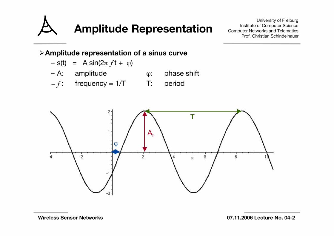
Amplitude Representation

Amplitude representation of a sinus curve– s(t) = A sin(2π f t + ϕ)

– A: amplitude ϕ: phase shift– f : frequency = 1/T T: period

At

ϕ

T




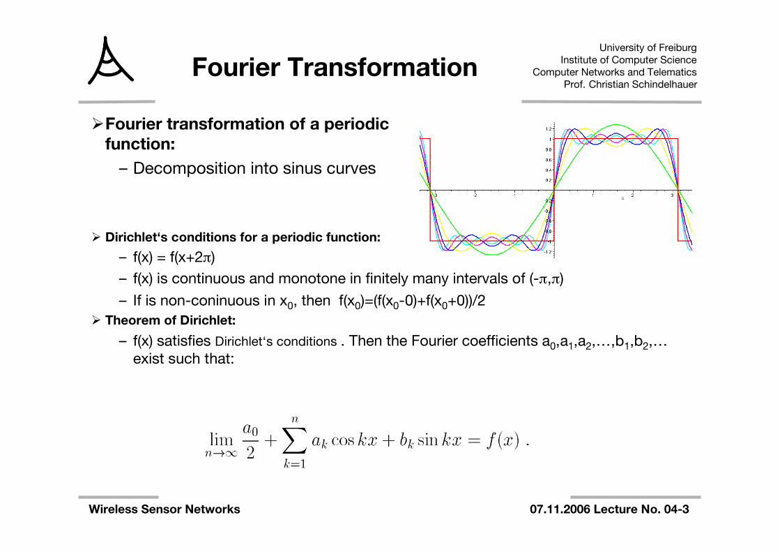
Fourier Transformation

Fourier transformation of a periodicfunction:

– Decomposition into sinus curves

Dirichlet‘s conditions for a periodic function:

– f(x) = f(x+2π)– f(x) is continuous and monotone in finitely many intervals of (-π,π)

– If is non-coninuous in x0, then f(x0)=(f(x0-0)+f(x0+0))/2 Theorem of Dirichlet:

– f(x) satisfies Dirichlet‘s conditions . Then the Fourier coefficients a0,a1,a2,…,b1,b2,…exist such that:




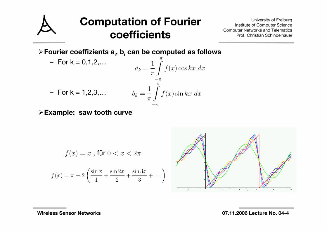
Computation of Fouriercoefficients

Fourier coeffizients ai, bi can be computed as follows– For k = 0,1,2,…

– For k = 1,2,3,…

Example: saw tooth curve




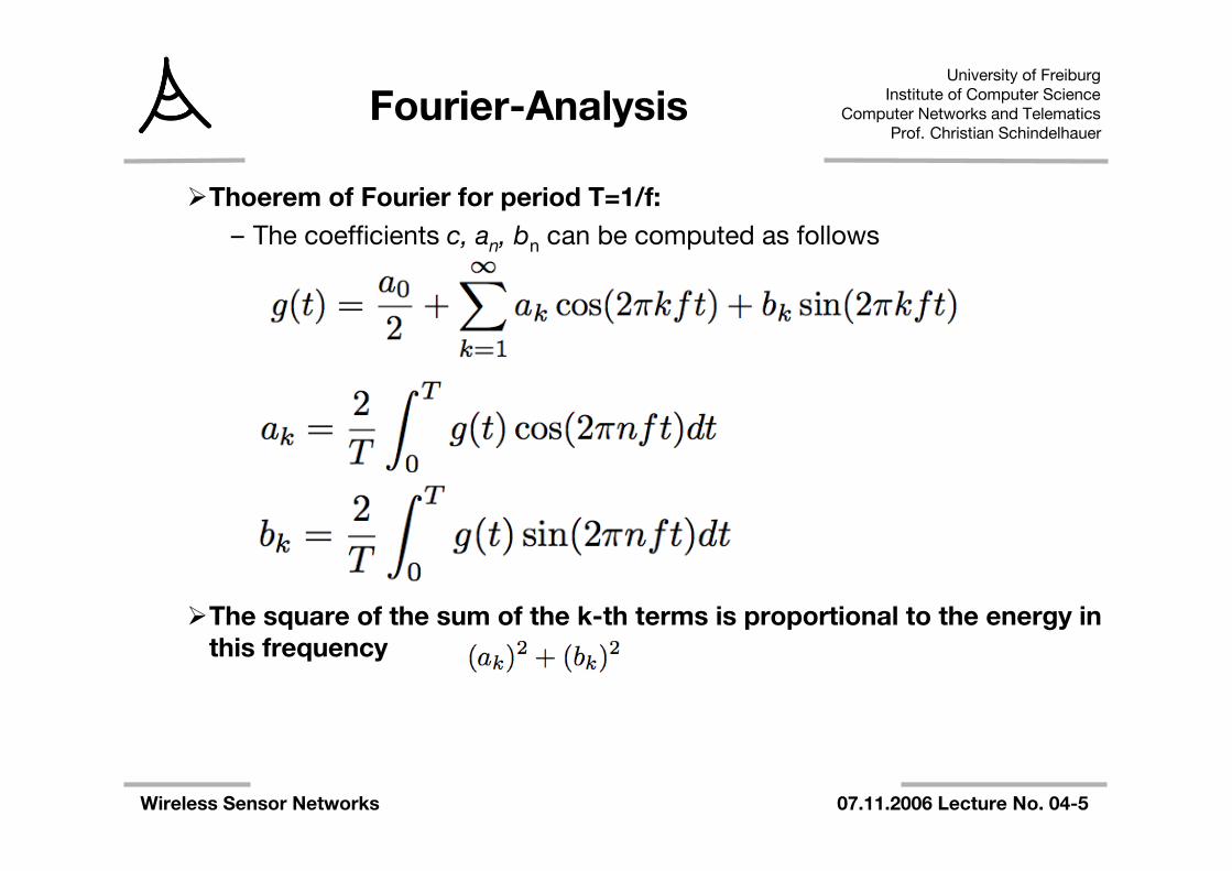
Fourier-Analysis

Thoerem of Fourier for period T=1/f:– The coefficients c, an, bn can be computed as follows

The square of the sum of the k-th terms is proportional to the energy inthis frequency




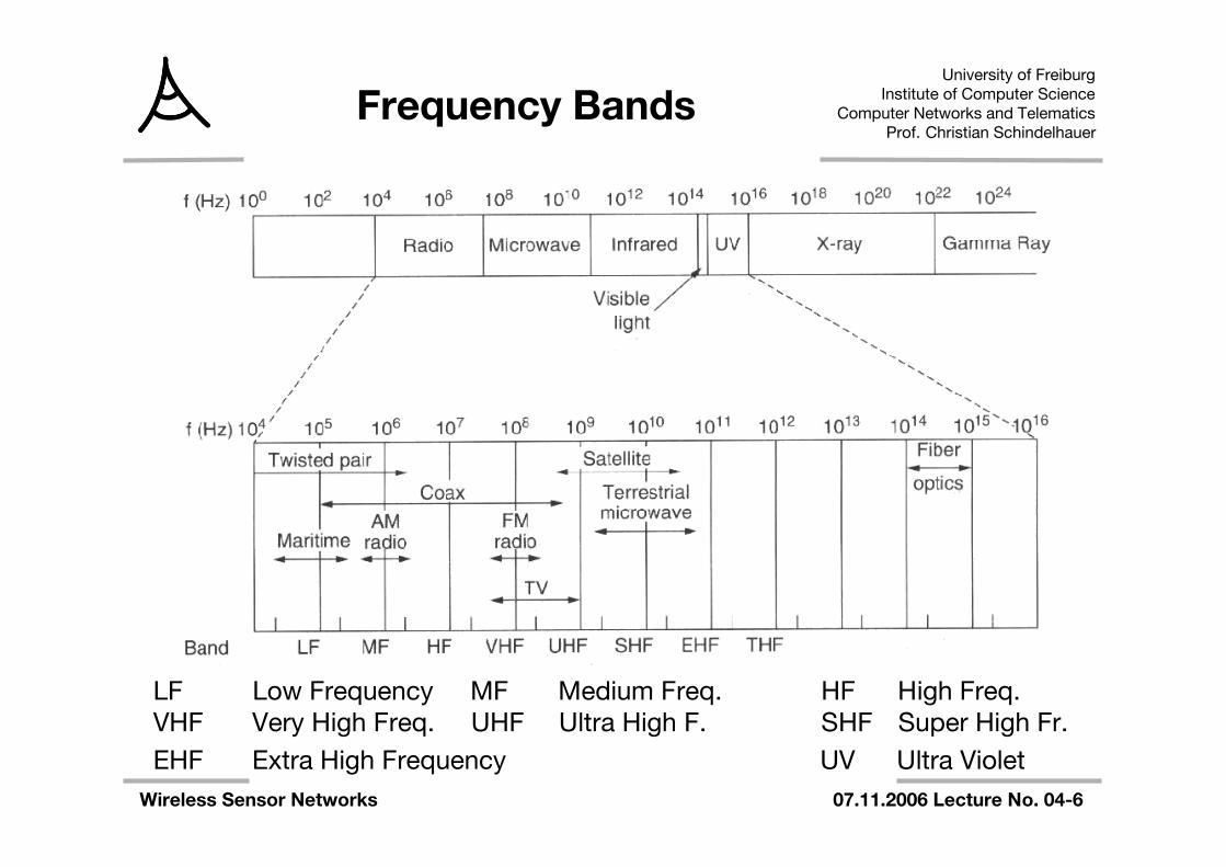
Frequency Bands

LF Low Frequency MF Medium Freq. HF High Freq.VHF Very High Freq. UHF Ultra High F. SHF Super High Fr.EHF Extra High Frequency UV Ultra Violet




Radio Propagation

Propagation on straight lineSignal strength is proportional to 1/d² in free space

– In practice can be modeled by 1/dc, for c up to 4 or 5Energy consumption

– for transmitting a radio signal over distance d in empty space is d²Basic properties

– Reflection– Refraction (between media with slower speed of propagation)– Interference– Diffraction– Attenuation in air (especially HV, VHF)




Radio Propagation

VLF, LF, MF– follow the curvature of the globe (up zu 1000 kms in VLF)– pass through buildings

HF, VHF– absorbed by earth– reflected by ionosphere in a height of 100-500 km

>100 MHz– No passing through walls– Good focus

> 8 GHz absorption by rain




Radio Propagation

Multiple Path Fading– Because of reflection, diffraction and diffusion the signal arrives on

multiple paths– Phase shifts because of different path length causes interferences

Problems with mobile nodes– Fast Fading

• Different transmission paths• Different phase shifts

– Slow Fading• Increasing or decreasing the distance between sender and receiver




Signal Interference NoiseRatio

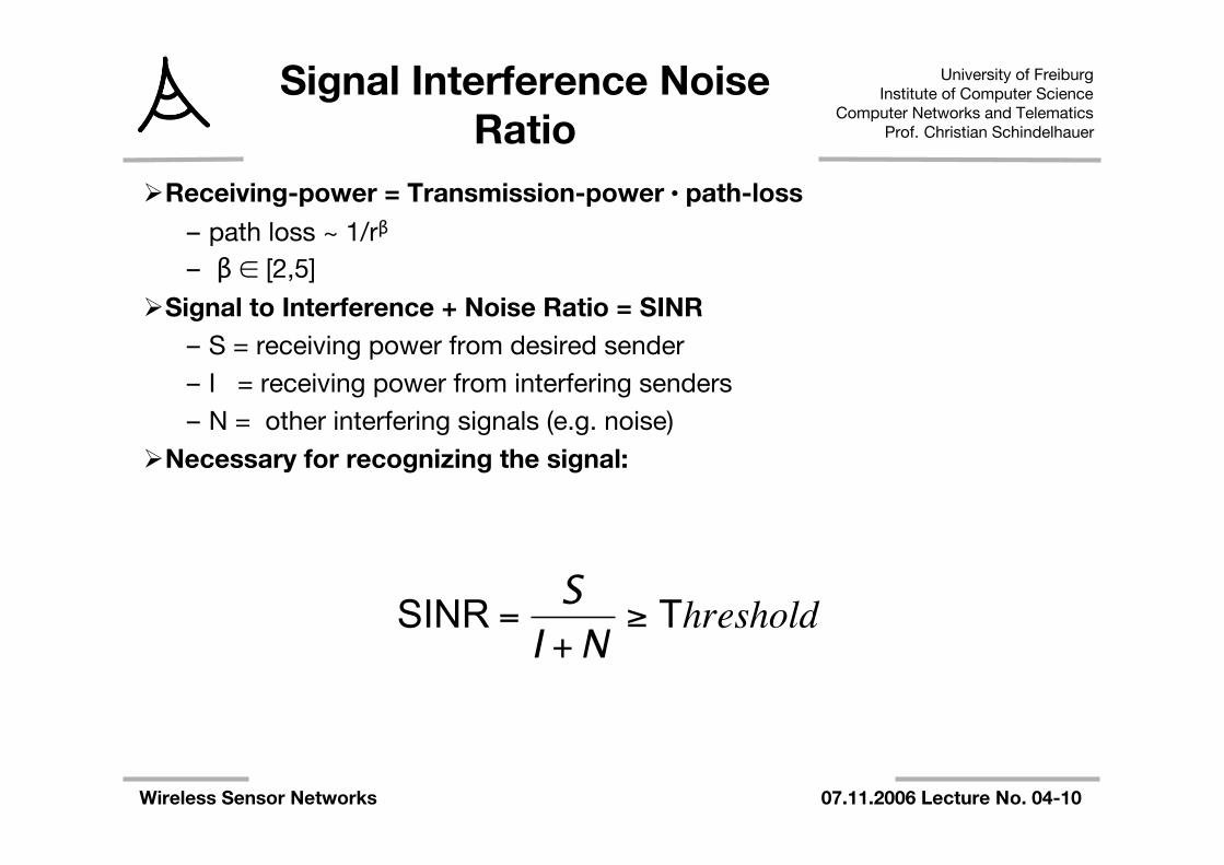
Receiving-power = Transmission-power ⋅ path-loss

– path loss ~ 1/rβ

– β ∈ [2,5]

Signal to Interference + Noise Ratio = SINR– S = receiving power from desired sender– I = receiving power from interfering senders– N = other interfering signals (e.g. noise)

Necessary for recognizing the signal:

!

SINR =S

I + N" Threshold




Frequency allocation

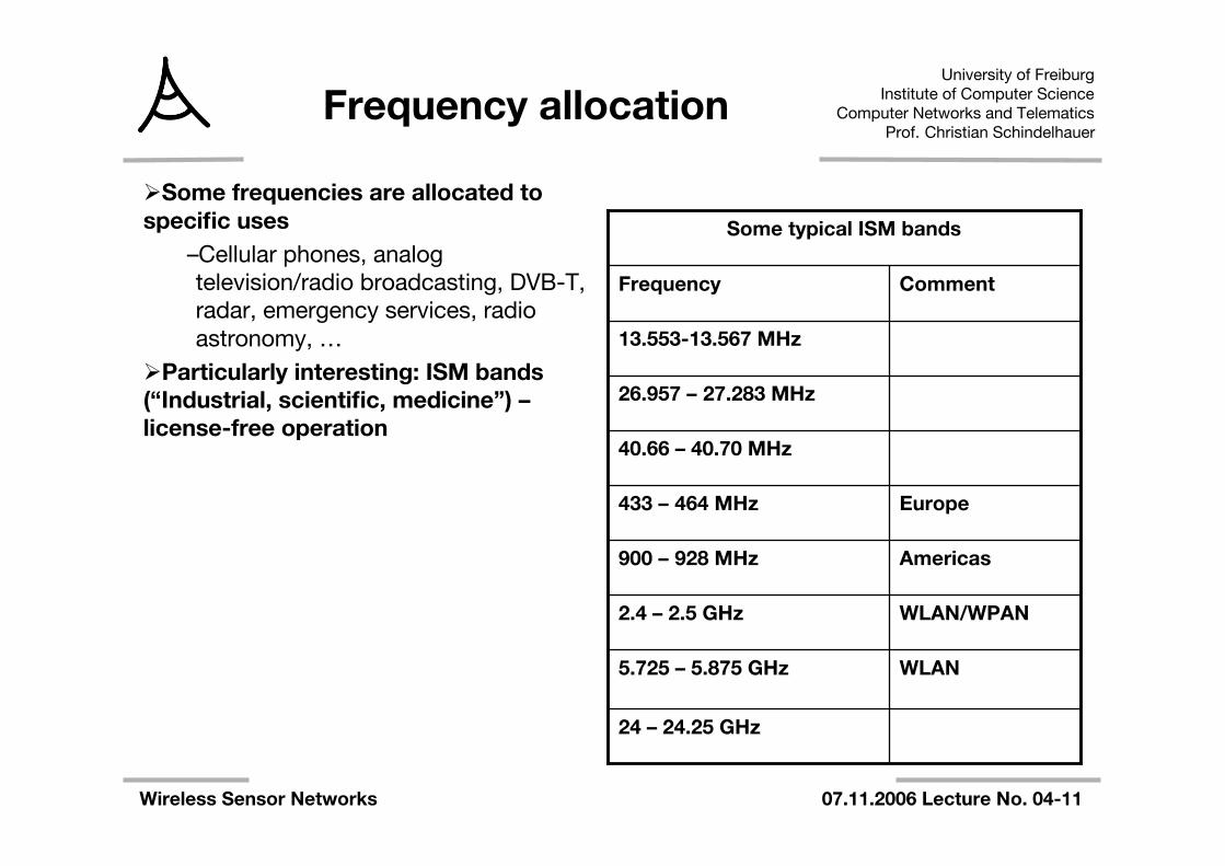
Some frequencies are allocated tospecific uses

–Cellular phones, analogtelevision/radio broadcasting, DVB-T,radar, emergency services, radioastronomy, …

Particularly interesting: ISM bands(“Industrial, scientific, medicine”) –license-free operation

Some typical ISM bands

24 – 24.25 GHz

WLAN5.725 – 5.875 GHz

WLAN/WPAN2.4 – 2.5 GHz

Americas900 – 928 MHz

Europe433 – 464 MHz

40.66 – 40.70 MHz

26.957 – 27.283 MHz

13.553-13.567 MHz

CommentFrequency




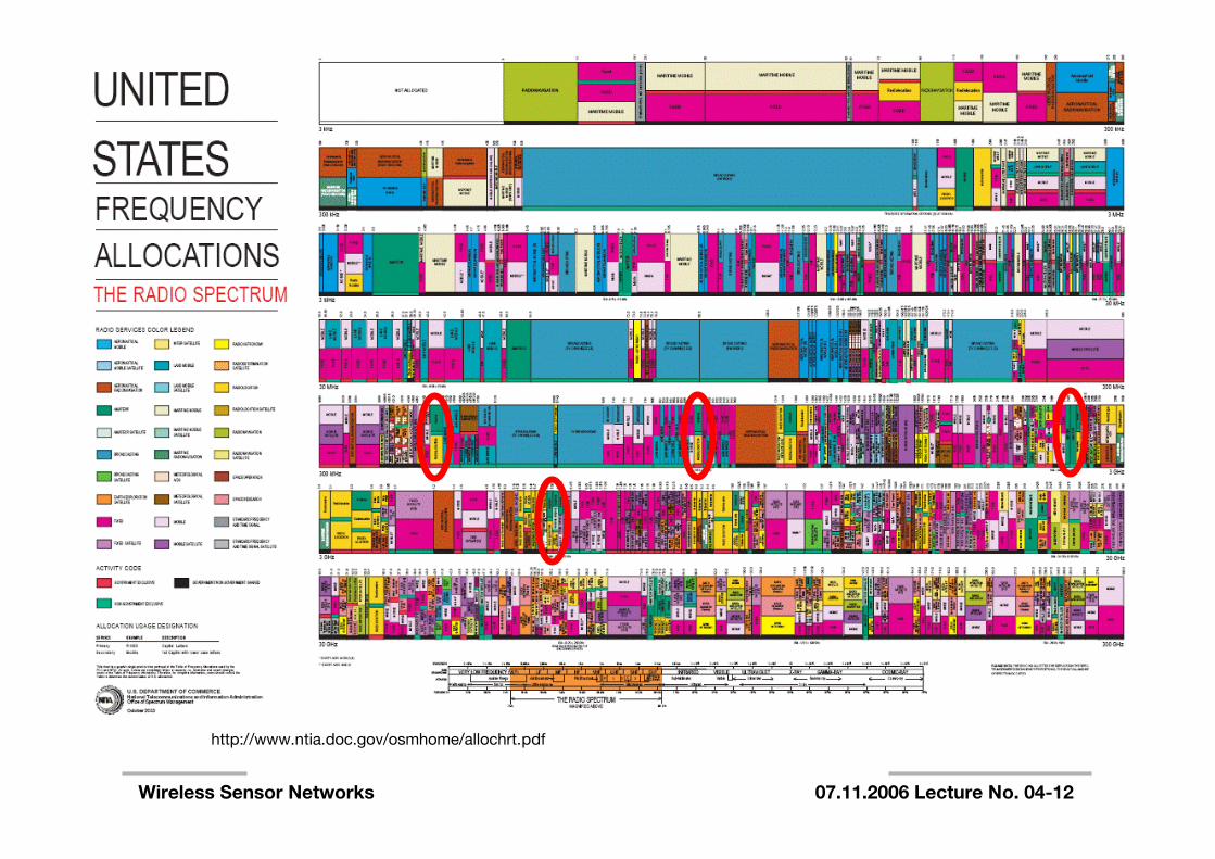
Example: US frequencyallocation

http://www.ntia.doc.gov/osmhome/allochrt.pdf




Transceivers and thePhysical Layer

Frequency bandsModulationSignal distortion – wireless channelsFrom waves to bitsChannel modelsTransceiver design




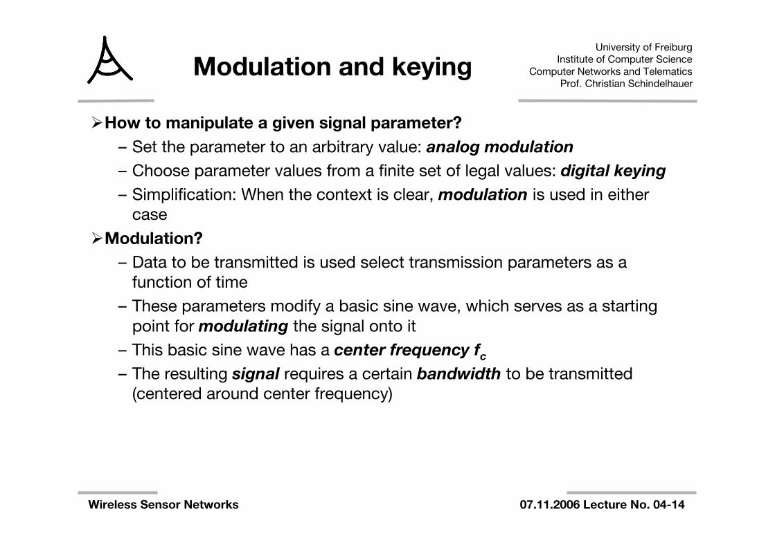
Modulation and keying

How to manipulate a given signal parameter?– Set the parameter to an arbitrary value: analog modulation– Choose parameter values from a finite set of legal values: digital keying– Simplification: When the context is clear, modulation is used in either

caseModulation?

– Data to be transmitted is used select transmission parameters as afunction of time

– These parameters modify a basic sine wave, which serves as a startingpoint for modulating the signal onto it

– This basic sine wave has a center frequency fc

– The resulting signal requires a certain bandwidth to be transmitted(centered around center frequency)




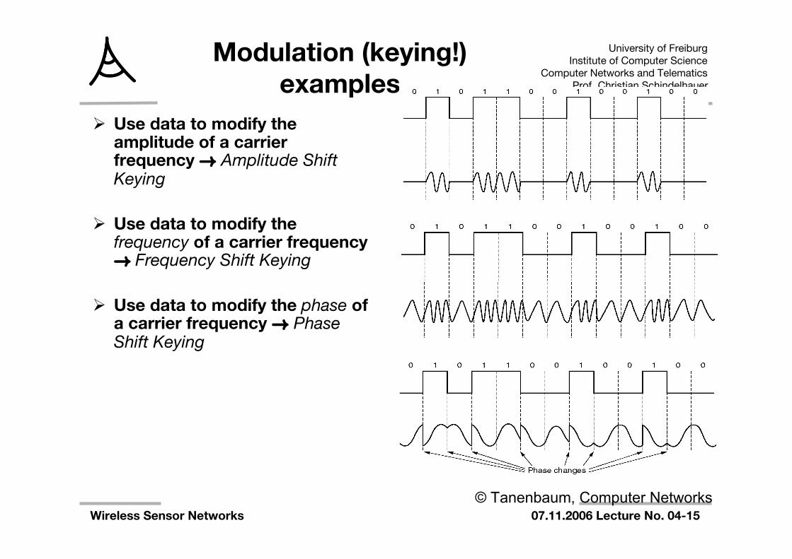
Modulation (keying!)examples

Use data to modify theamplitude of a carrierfrequency ! Amplitude ShiftKeying

Use data to modify thefrequency of a carrier frequency! Frequency Shift Keying

Use data to modify the phase ofa carrier frequency ! PhaseShift Keying

© Tanenbaum, Computer Networks




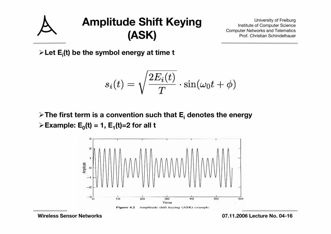
Amplitude Shift Keying(ASK)

Let Ei(t) be the symbol energy at time t

The first term is a convention such that Ei denotes the energyExample: E0(t) = 1, E1(t)=2 for all t




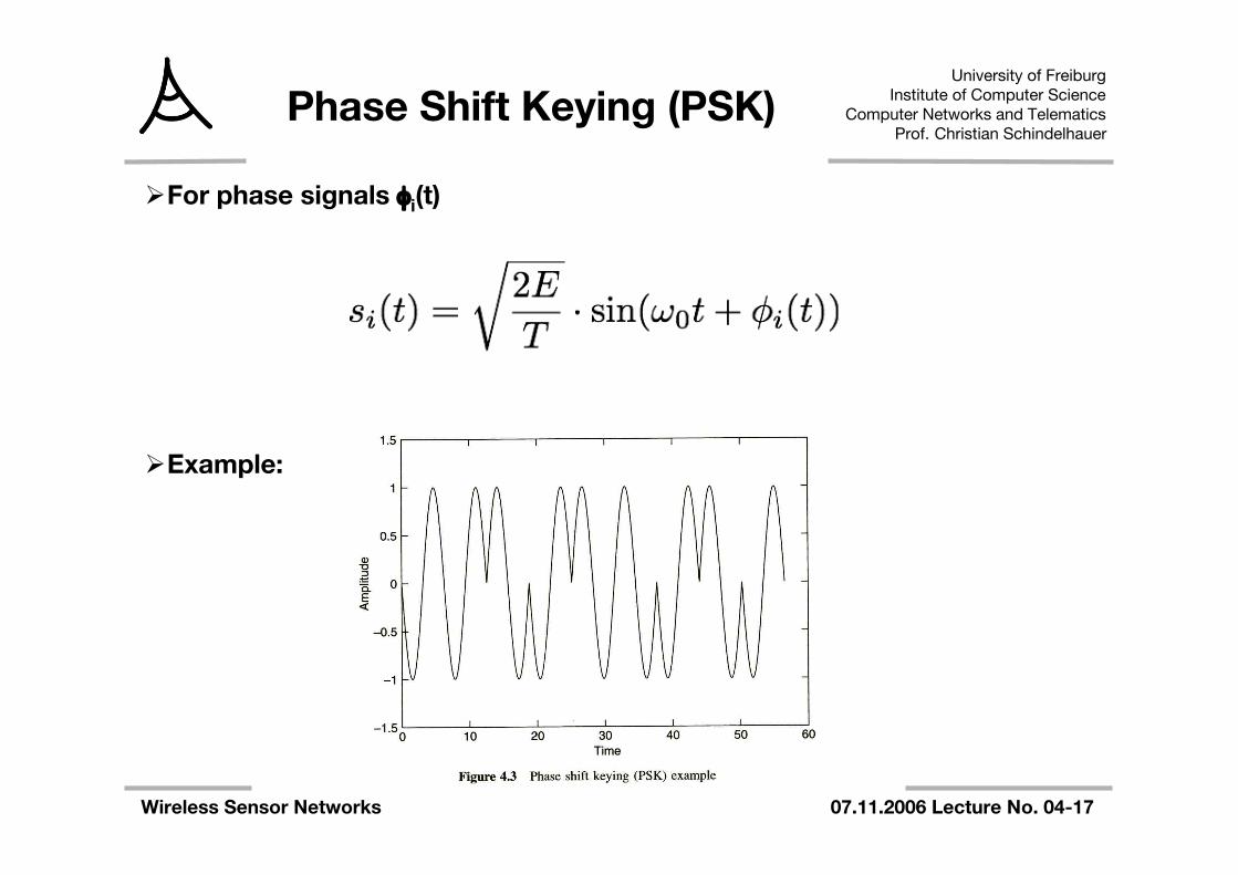
Phase Shift Keying (PSK)

For phase signals φi(t)

Example:




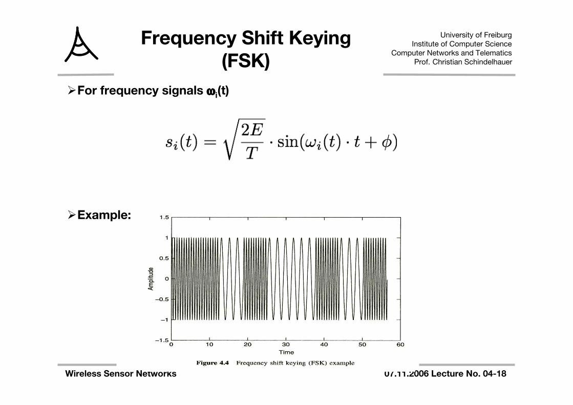
Frequency Shift Keying(FSK)

For frequency signals ωi(t)

Example:




Receiver: Demodulation

The receiver looks at the received wave form and matches it with thedata bit that caused the transmitter to generate this wave form

– Necessary: one-to-one mapping between data and wave form– Because of channel imperfections, this is at best possible for digital

signals, but not for analog signalsProblems caused by

– Carrier synchronization: frequency can vary between sender and receiver(drift, temperature changes, aging, …)

– Bit synchronization (actually: symbol synchronization): When does symbolrepresenting a certain bit start/end?

– Frame synchronization: When does a packet start/end?– Biggest problem: Received signal is not the transmitted signal!




Overview





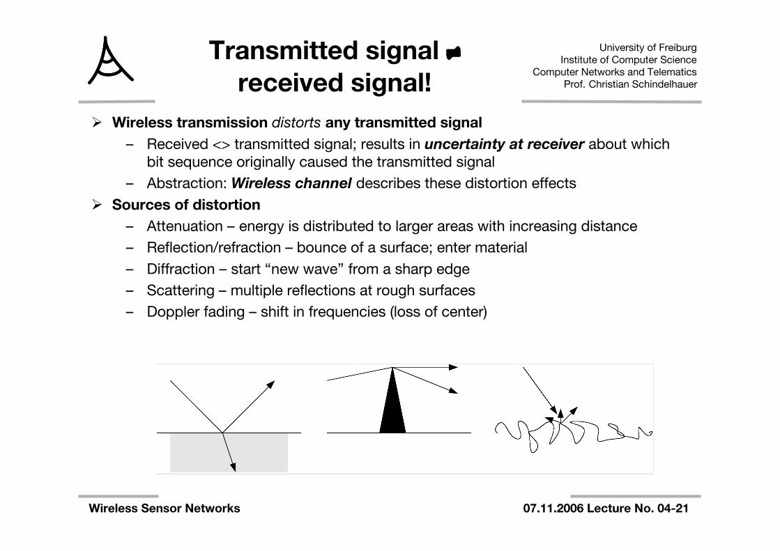
Transmitted signal ≠received signal!

Wireless transmission distorts any transmitted signal– Received <> transmitted signal; results in uncertainty at receiver about which

bit sequence originally caused the transmitted signal– Abstraction: Wireless channel describes these distortion effects

Sources of distortion– Attenuation – energy is distributed to larger areas with increasing distance– Reflection/refraction – bounce of a surface; enter material– Diffraction – start “new wave” from a sharp edge– Scattering – multiple reflections at rough surfaces– Doppler fading – shift in frequencies (loss of center)




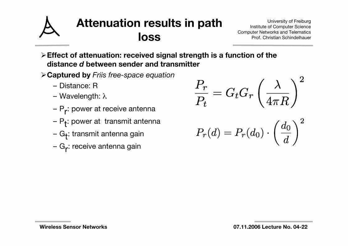
Attenuation results in pathloss

Effect of attenuation: received signal strength is a function of thedistance d between sender and transmitter

Captured by Friis free-space equation– Distance: R– Wavelength: λ

– Pr: power at receive antenna

– Pt: power at transmit antenna

– Gt: transmit antenna gain

– Gr: receive antenna gain




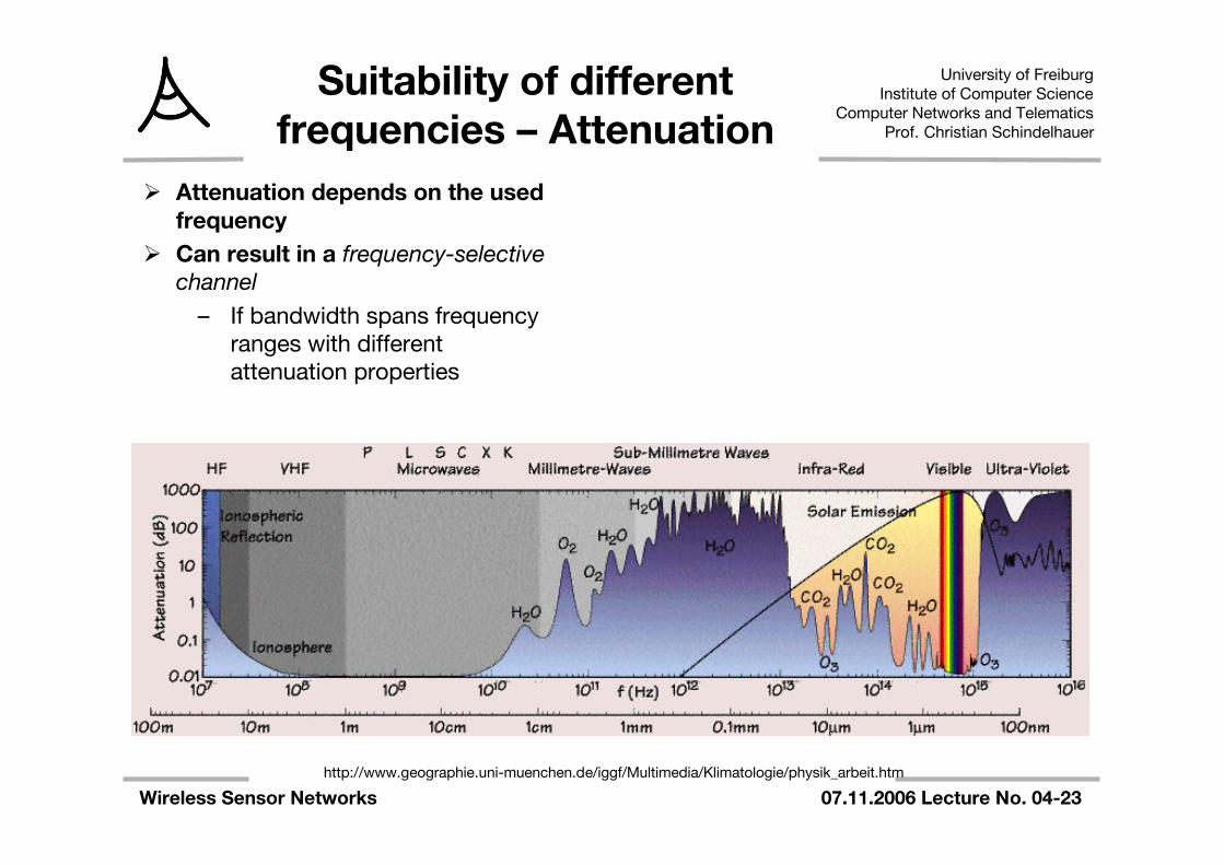
Suitability of differentfrequencies – Attenuation

Attenuation depends on the usedfrequency

Can result in a frequency-selectivechannel

– If bandwidth spans frequencyranges with differentattenuation properties

http://www.geographie.uni-muenchen.de/iggf/Multimedia/Klimatologie/physik_arbeit.htm




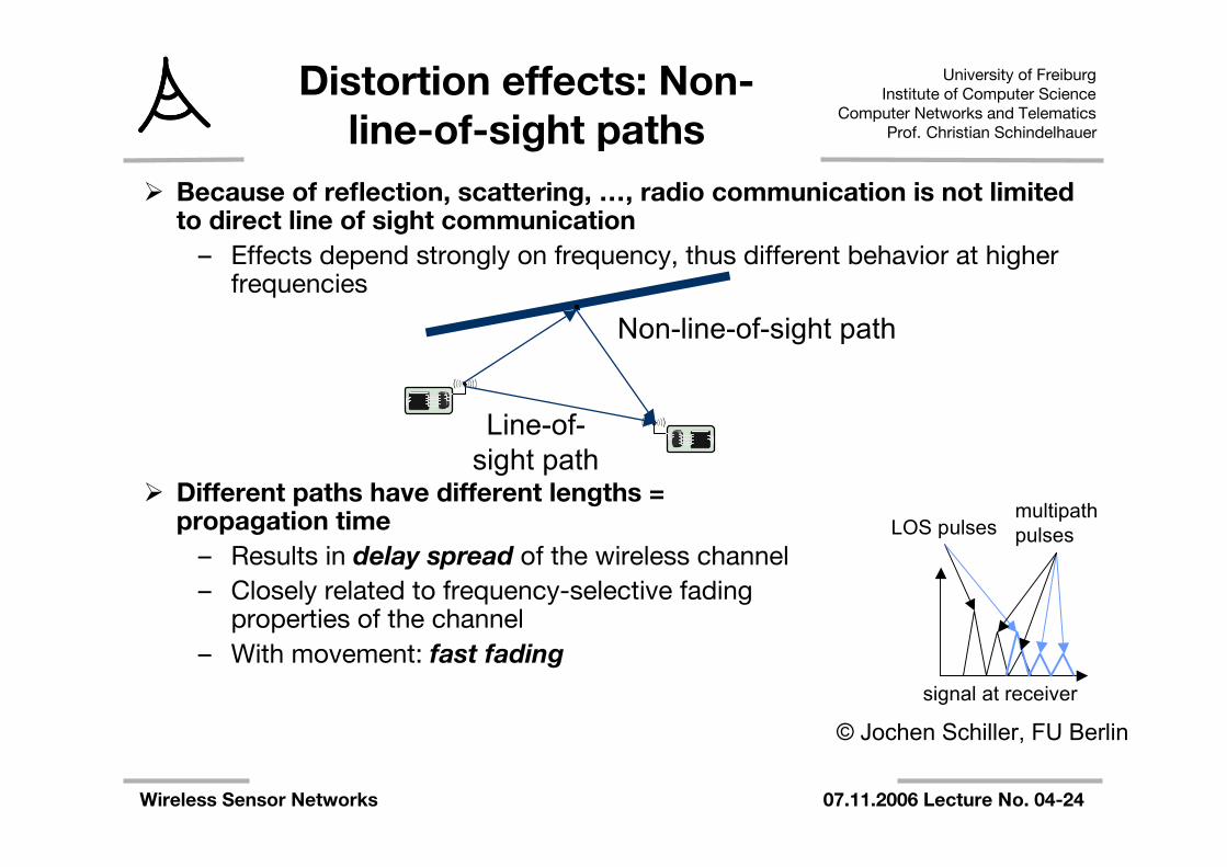
Distortion effects: Non-line-of-sight paths

Because of reflection, scattering, …, radio communication is not limitedto direct line of sight communication

– Effects depend strongly on frequency, thus different behavior at higherfrequencies

Different paths have different lengths =propagation time

– Results in delay spread of the wireless channel– Closely related to frequency-selective fading

properties of the channel– With movement: fast fading

Line-of-sight path

Non-line-of-sight path

signal at receiver

LOS pulsesmultipathpulses

© Jochen Schiller, FU Berlin




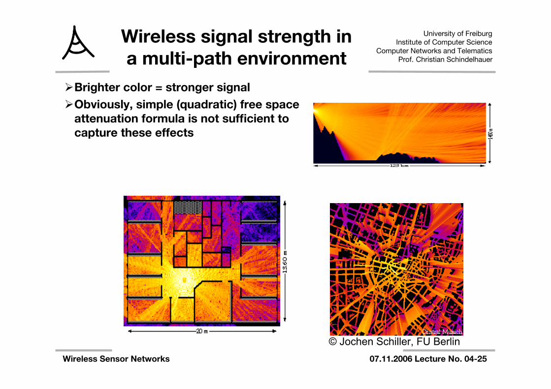
Wireless signal strength ina multi-path environment

Brighter color = stronger signalObviously, simple (quadratic) free space

attenuation formula is not sufficient tocapture these effects

© Jochen Schiller, FU Berlin




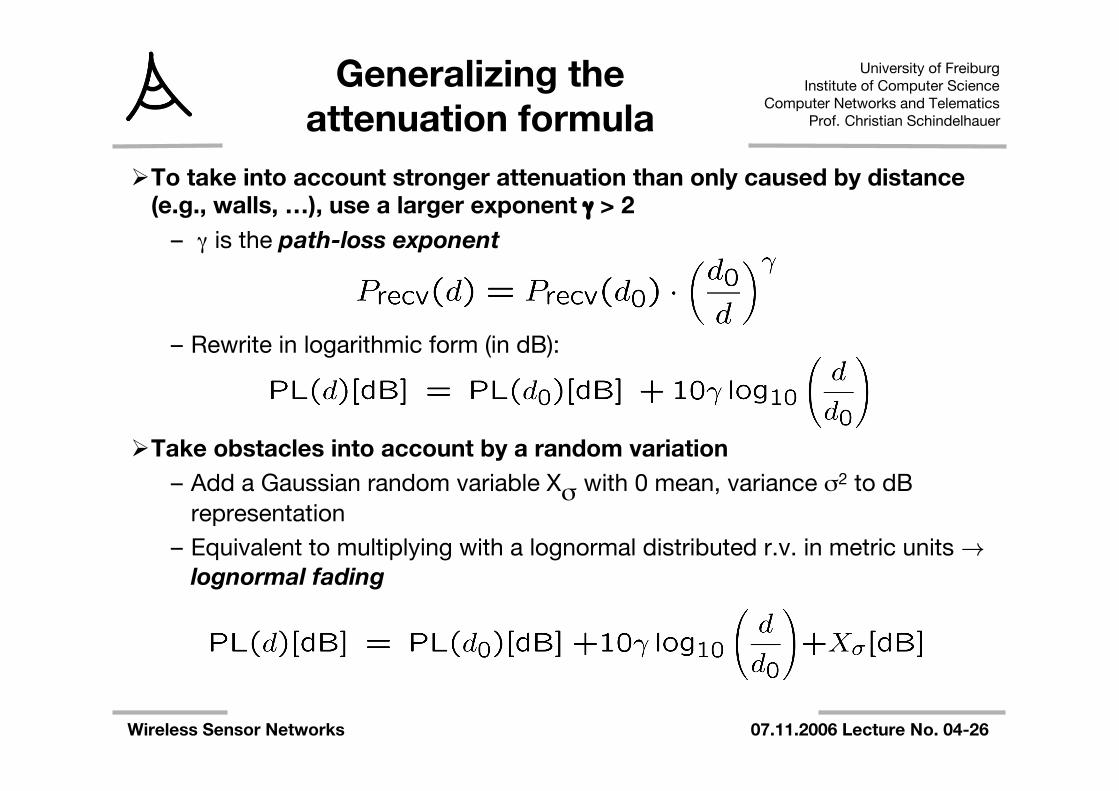
To take into account stronger attenuation than only caused by distance(e.g., walls, …), use a larger exponent γ > 2

– γ is the path-loss exponent

– Rewrite in logarithmic form (in dB):

Take obstacles into account by a random variation– Add a Gaussian random variable Xσ with 0 mean, variance σ2 to dB

representation– Equivalent to multiplying with a lognormal distributed r.v. in metric units !

lognormal fading

Generalizing theattenuation formula




Transceivers and thePhysical Layer





Noise and interference

So far: only a single transmitter assumed– Only disturbance: self-interference of a signal with multi-path “copies” of

itself In reality, two further disturbances

– Noise – due to effects in receiver electronics, depends on temperature• Typical model: an additive Gaussian variable, mean 0, no correlation

in time– Interference from third parties

• Co-channel interference: another sender uses the same spectrum• Adjacent-channel interference: another sender uses some other part

of the radio spectrum, but receiver filters are not good enough tofully suppress it

Effect: Received signal is distorted by channel, corrupted by noise andinterference

– What is the result on the received bits?




Symbols and bit errors

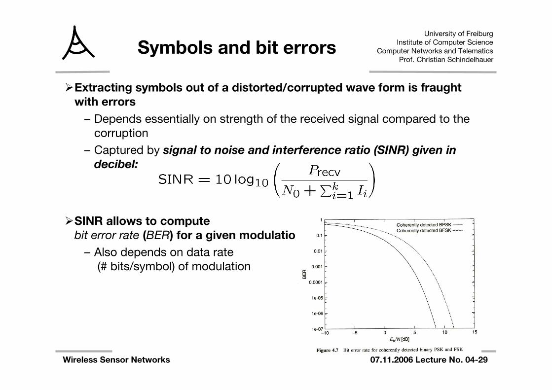
Extracting symbols out of a distorted/corrupted wave form is fraughtwith errors

– Depends essentially on strength of the received signal compared to thecorruption

– Captured by signal to noise and interference ratio (SINR) given indecibel:

SINR allows to computebit error rate (BER) for a given modulation

– Also depends on data rate (# bits/symbol) of modulation




Overview





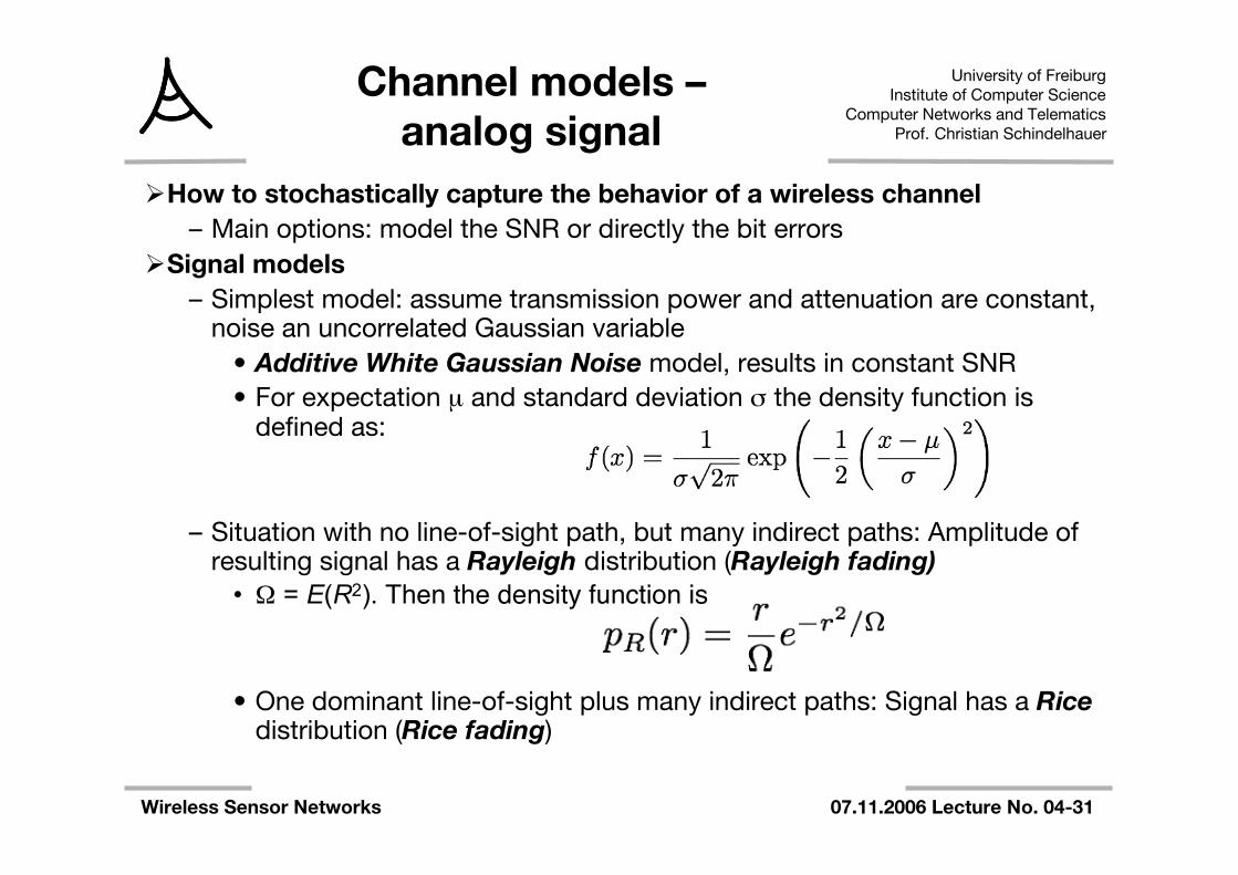
Channel models –analog signal

How to stochastically capture the behavior of a wireless channel– Main options: model the SNR or directly the bit errors

Signal models– Simplest model: assume transmission power and attenuation are constant,

noise an uncorrelated Gaussian variable• Additive White Gaussian Noise model, results in constant SNR• For expectation µ and standard deviation σ the density function is

defined as:

– Situation with no line-of-sight path, but many indirect paths: Amplitude ofresulting signal has a Rayleigh distribution (Rayleigh fading)

• Ω = E(R2). Then the density function is

• One dominant line-of-sight plus many indirect paths: Signal has a Ricedistribution (Rice fading)




Channel models – digital

Directly model the resulting bit error behavior– Each bit is erroneous with constant probability, independent of the other

bits ! binary symmetric channel (BSC)– Capture fading models’ property that channel be in different states !

Markov models – states with different BERs• Example: Gilbert-Elliot model with “bad” and “good” channel states

and high/low bit error rates

– Fractal channel models describe number of (in-)correct bits in a row by aheavy-tailed distribution

good bad




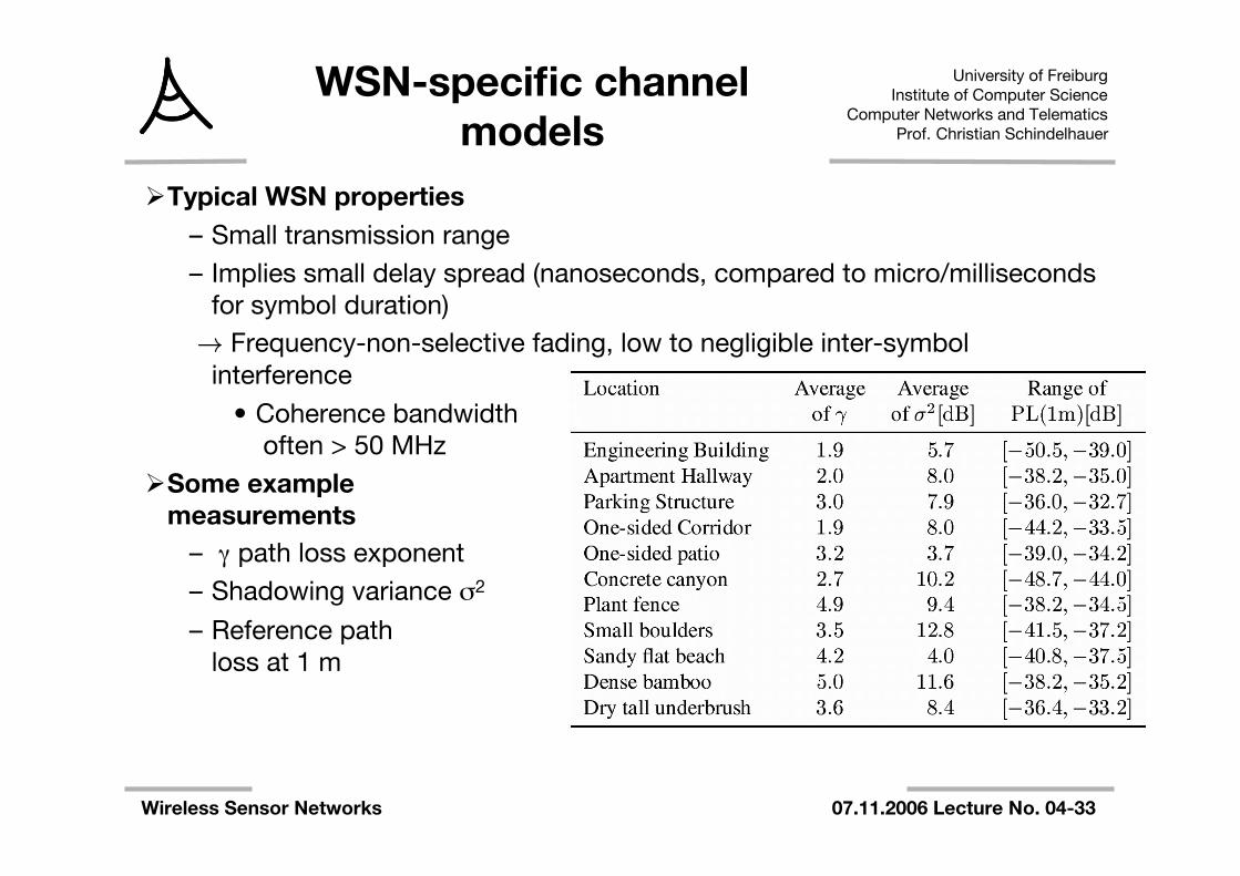
WSN-specific channelmodels

Typical WSN properties– Small transmission range– Implies small delay spread (nanoseconds, compared to micro/milliseconds

for symbol duration) ! Frequency-non-selective fading, low to negligible inter-symbol

interference• Coherence bandwidth

often > 50 MHzSome example

measurements– γ path loss exponent– Shadowing variance σ2

– Reference pathloss at 1 m




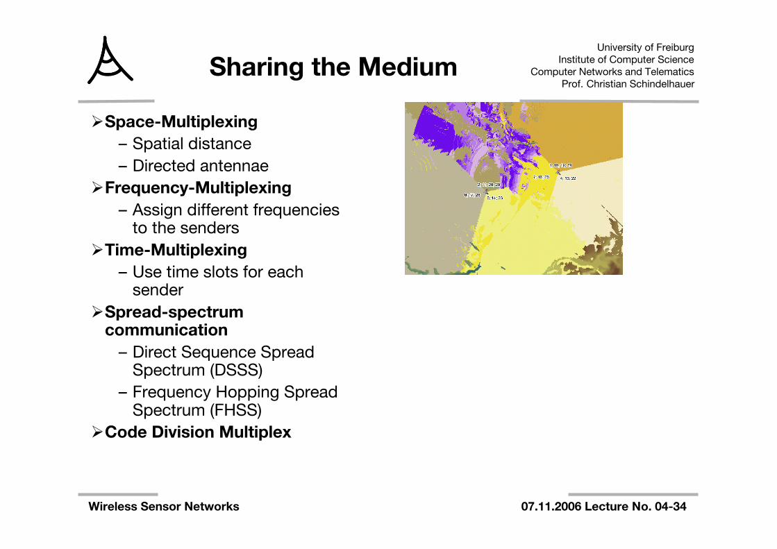
Sharing the Medium

Space-Multiplexing– Spatial distance– Directed antennae

Frequency-Multiplexing– Assign different frequencies

to the sendersTime-Multiplexing

– Use time slots for eachsender

Spread-spectrumcommunication

– Direct Sequence SpreadSpectrum (DSSS)

– Frequency Hopping SpreadSpectrum (FHSS)

Code Division Multiplex




Frequency HoppingSpread Spectrum

Change the frequency while transfering the signal– Invented by Hedy Lamarr, George Antheil

Slow hopping– Change the frequency slower than the signals

comeFast hopping

– Change the frequency faster

36

University of FreiburgComputer Networks and Telematics

Prof. Christian Schindelhauer

Thank you(and thanks go also to Holger Karl for providing some slides)

Wireless Sensor NetworksChristian Schindelhauer

4th Lecture07.11.2006

[email protected]

Wireless Sensor Networks - uni-freiburg.de

Documents

Transcript of Wireless Sensor Networks - uni-freiburg.de