Waves and Modern Physics PHY 123 - Spring 2012

1st Midterm Exam

Wednesday, February 22

Chapter 15 Wave Motion

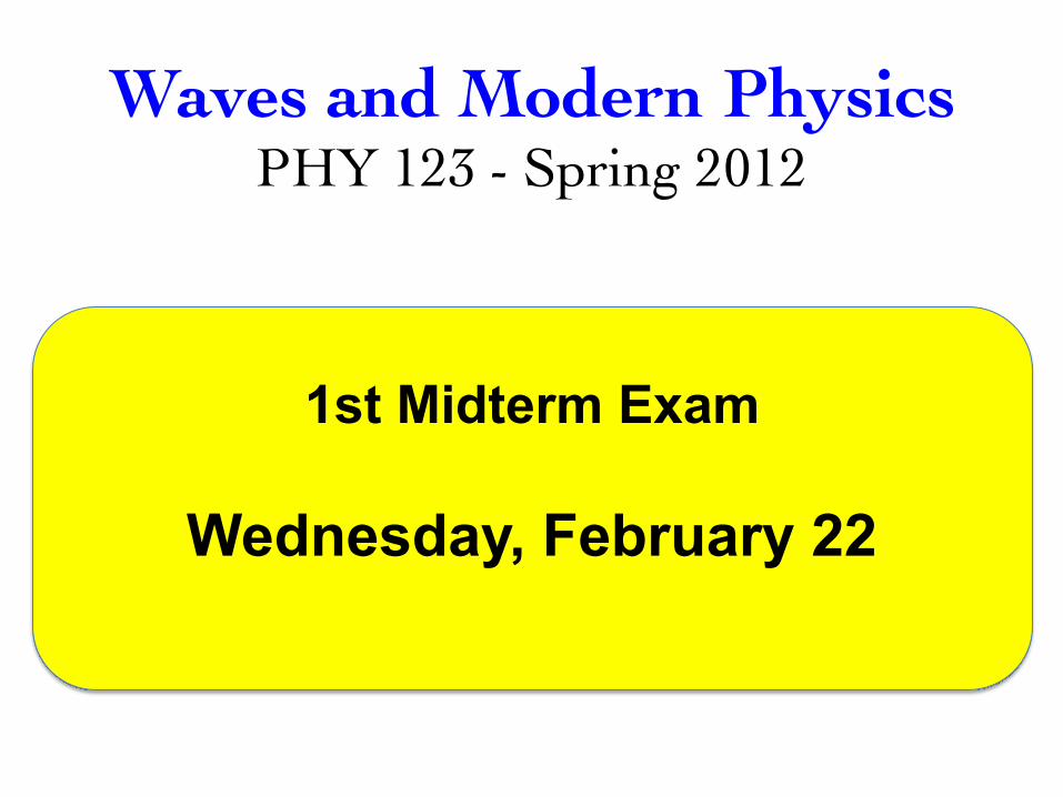
Interference: Adding waves

Mathematical representation:

A sin(kx −ωt) + A sin(kx +ωt) = 2A cos(ωt) sin(kx)

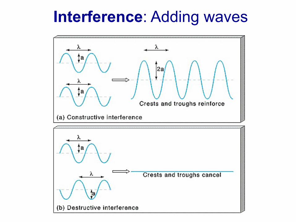
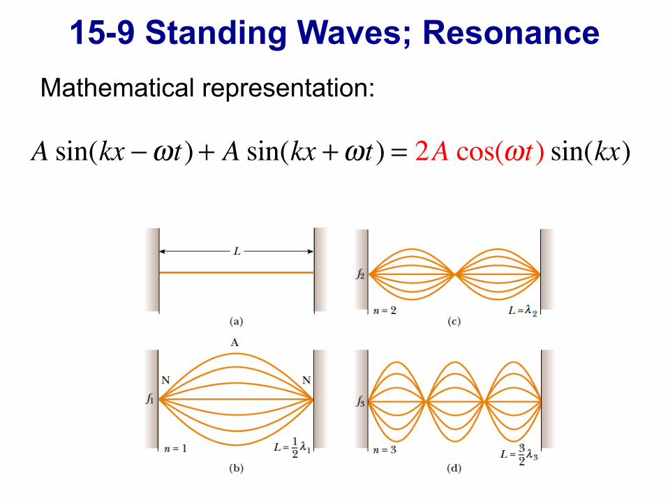
15-9 Standing Waves; Resonance

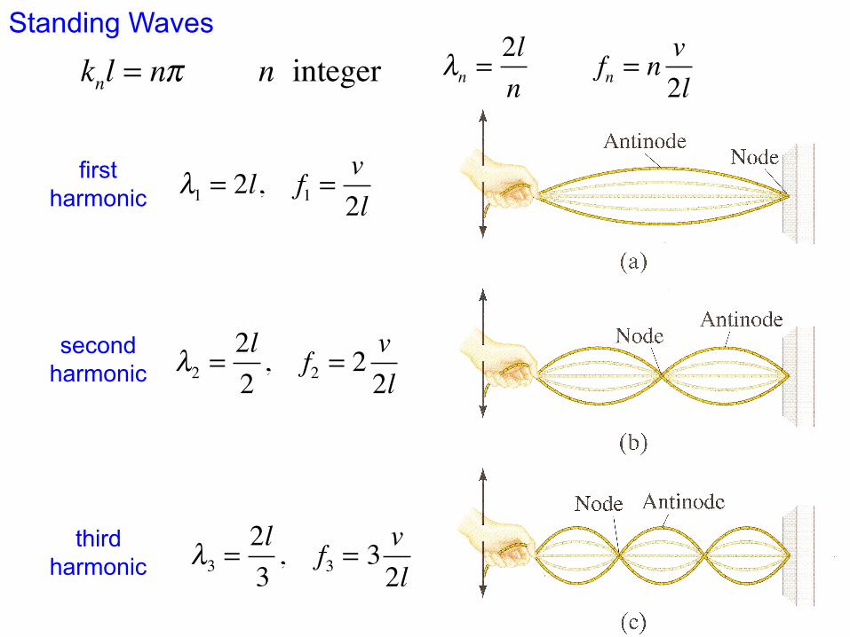
Standing Waves

knl = nπ n integer

λ1 = 2l, f1 =v2l

λn =2ln

fn = nv2l

first harmonic

second harmonic λ2 =

2l2, f2 = 2

v2l

third harmonic λ3 =

2l3, f3 = 3

v2l

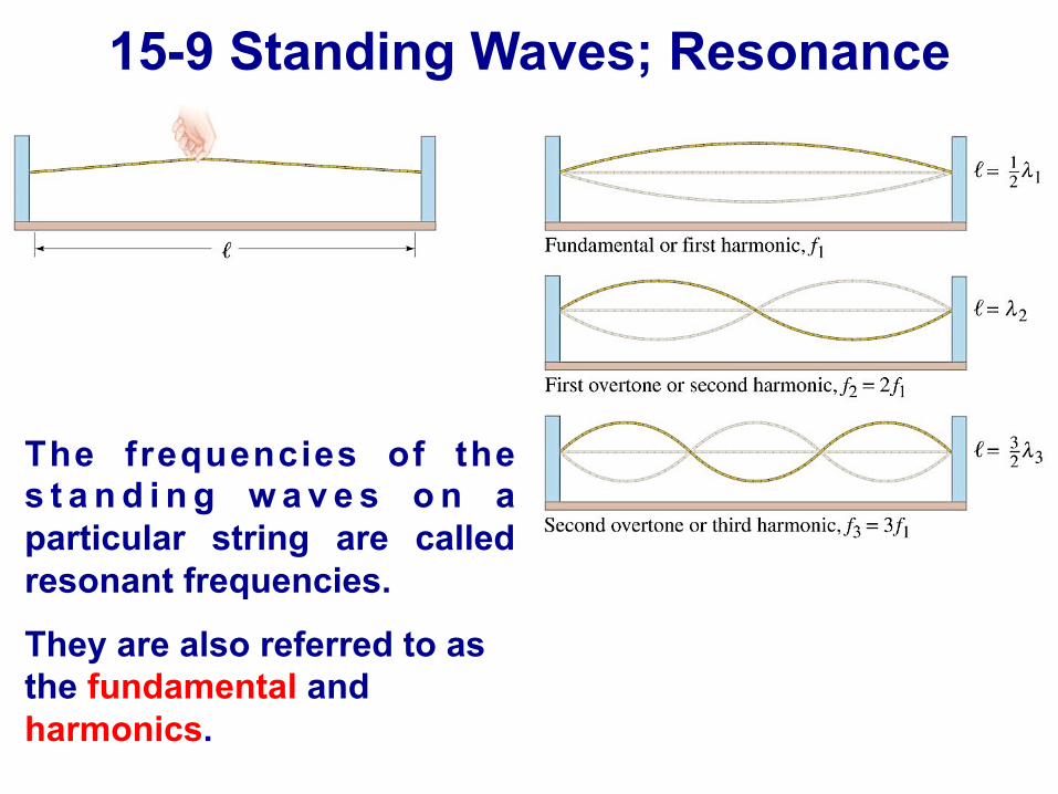
The frequencies of the s t a n d i n g w a v e s o n a particular string are called resonant frequencies.

They are also referred to as the fundamental and harmonics.

15-9 Standing Waves; Resonance

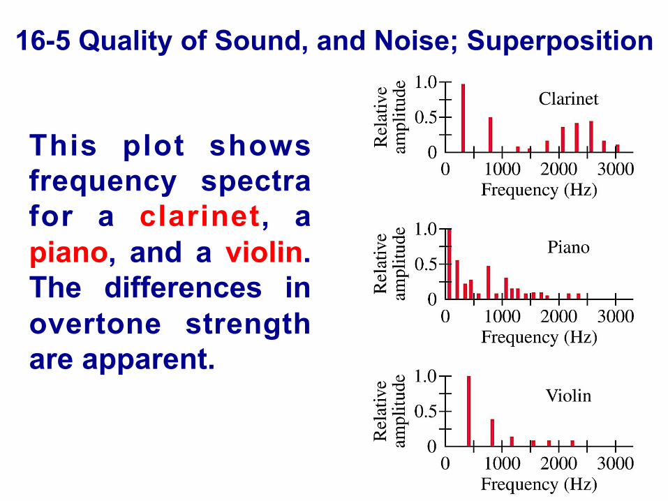
This plot shows frequency spectra for a clarinet, a piano, and a violin. The differences in overtone strength are apparent.

16-5 Quality of Sound, and Noise; Superposition

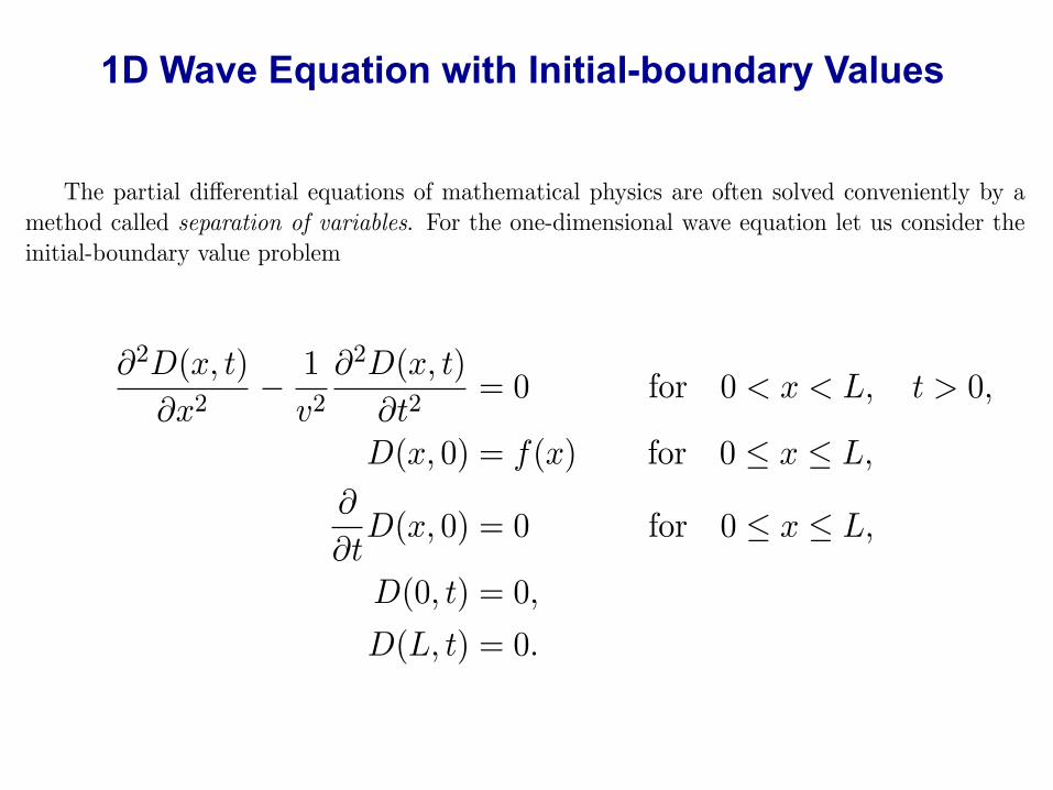
1D Wave Equation with Initial-boundary Values The one-dimensional wave equation with initial-boundary values

The partial di�erential equations of mathematical physics are often solved conveniently by amethod called separation of variables. For the one-dimensional wave equation let us consider theinitial-boundary value problem

�2D(x, t)�x2

� 1v2

�2D(x, t)�t2

= 0 for 0 < x < L, t > 0,

D(x, 0) = f(x) for 0 x L,

�

�tD(x, 0) = 0 for 0 x L,

D(0, t) = 0,D(L, t) = 0.

We seek solutions of the di�erential equation of the form D(x, t) = X(x)T (t). Substituting thisD(x, t) in the wave equation, dividing by D(x, t), and transposing, we find

T00(t)

T (t)= v2 X

00(x)X(x)

.

Because the left-hand side of this equation depends only upon t and the right-end side is independentof t, both sides of this equation must equal the same constant. We say that the wave equation isseparable. Let us call this constant �⇥2. The homogeneous initial and boundary conditions give

v2X00

+ ⇥2X = 0,

X(0) = X(L) = 0,

T00

+ ⇥2T = 0,

T0(0) = 0.

We now find the eigenvalues⇥n

v= kn =

n�

L

and the eigenfunctions Xn = sin (n�x/L). Using these values of ⇥, we have

Tn = cosn�v

Lt

1

The one-dimensional wave equation with initial-boundary values

The partial di�erential equations of mathematical physics are often solved conveniently by amethod called separation of variables. For the one-dimensional wave equation let us consider theinitial-boundary value problem

�2D(x, t)�x2

� 1v2

�2D(x, t)�t2

= 0 for 0 < x < L, t > 0,

D(x, 0) = f(x) for 0 x L,

�

�tD(x, 0) = 0 for 0 x L,

D(0, t) = 0,D(L, t) = 0.

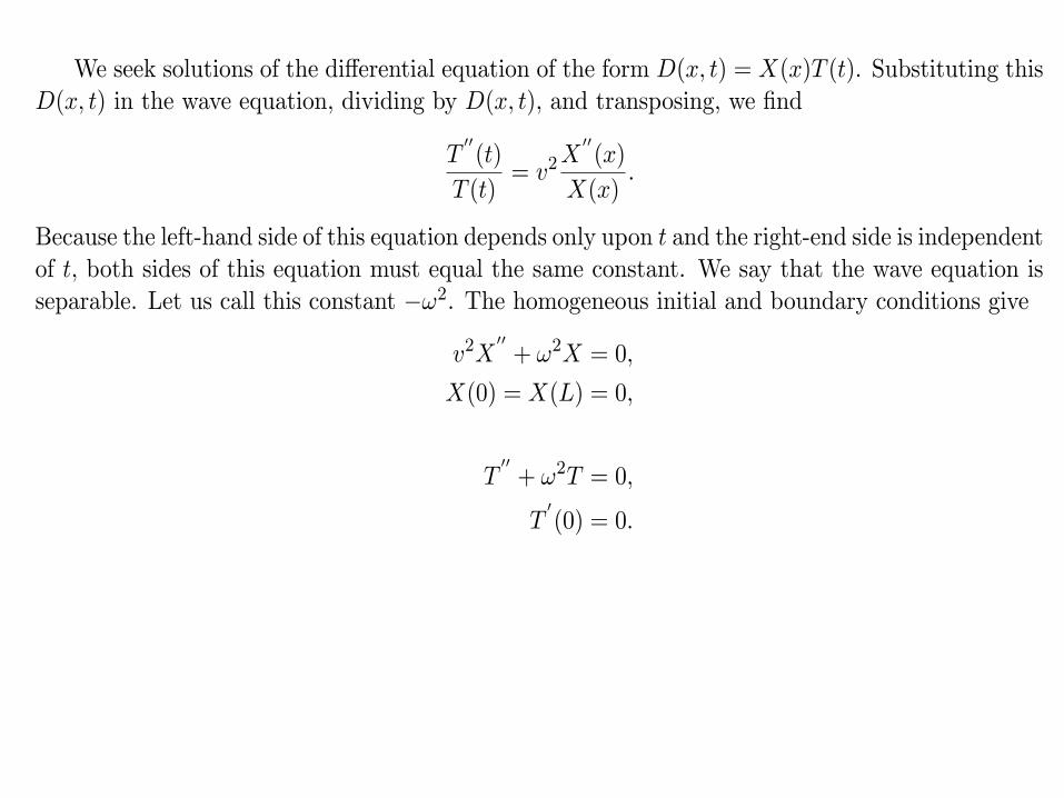
We seek solutions of the di�erential equation of the form D(x, t) = X(x)T (t). Substituting thisD(x, t) in the wave equation, dividing by D(x, t), and transposing, we find

T00(t)

T (t)= v2 X

00(x)X(x)

.

Because the left-hand side of this equation depends only upon t and the right-end side is independentof t, both sides of this equation must equal the same constant. We say that the wave equation isseparable. Let us call this constant �⇥2. The homogeneous initial and boundary conditions give

v2X00

+ ⇥2X = 0,

X(0) = X(L) = 0,

T00

+ ⇥2T = 0,

T0(0) = 0.

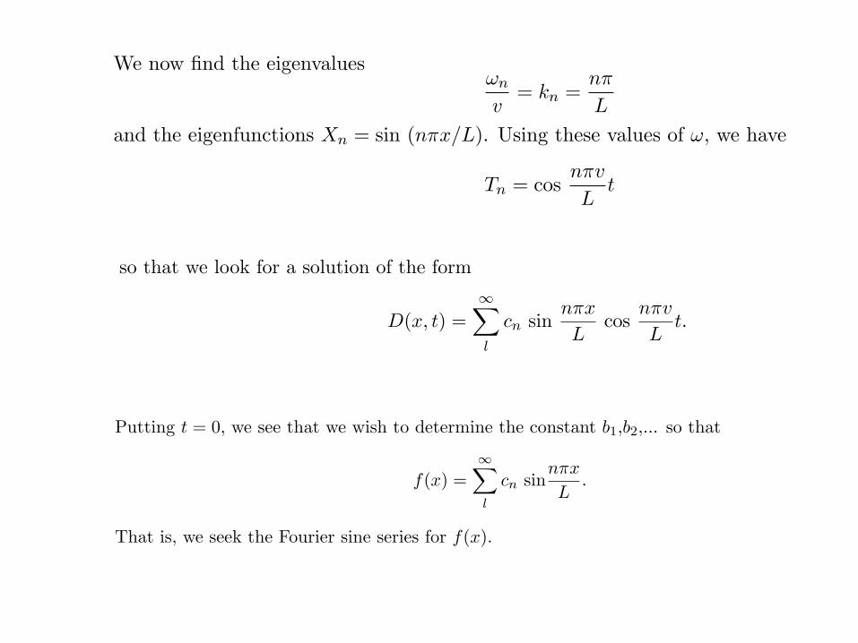
We now find the eigenvalues⇥n

v= kn =

n�

L

and the eigenfunctions Xn = sin (n�x/L). Using these values of ⇥, we have

Tn = cosn�v

Lt

1

The one-dimensional wave equation with initial-boundary values

The partial di�erential equations of mathematical physics are often solved conveniently by amethod called separation of variables. For the one-dimensional wave equation let us consider theinitial-boundary value problem

�2D(x, t)�x2

� 1v2

�2D(x, t)�t2

= 0 for 0 < x < L, t > 0,

D(x, 0) = f(x) for 0 x L,

�

�tD(x, 0) = 0 for 0 x L,

D(0, t) = 0,D(L, t) = 0.

We seek solutions of the di�erential equation of the form D(x, t) = X(x)T (t). Substituting thisD(x, t) in the wave equation, dividing by D(x, t), and transposing, we find

T00(t)

T (t)= v2 X

00(x)X(x)

.

Because the left-hand side of this equation depends only upon t and the right-end side is independentof t, both sides of this equation must equal the same constant. We say that the wave equation isseparable. Let us call this constant �⇥2. The homogeneous initial and boundary conditions give

v2X00

+ ⇥2X = 0,

X(0) = X(L) = 0,

T00

+ ⇥2T = 0,

T0(0) = 0.

We now find the eigenvalues⇥n

v= kn =

n�

L

and the eigenfunctions Xn = sin (n�x/L). Using these values of ⇥, we have

Tn = cosn�v

Lt

1

We consider the initial-boundary value problem for the one dimensional wave equation

@

2D(x, t)@x

2� 1

v

2

@

2D(x, t)@t

2= 0 for 0 < x < L, t > 0,

D(x, 0) = f(x) for 0 x L,

@

@t

D(x, 0) = 0 for 0 x L,

D(0, t) = 0,D(l, t) = 0.

We seek solutions of the di�erential equation of the form D(x, t) = X(x)T (t). Substituting thisD(x, t) in the wave equation, dividing by D(x, t), and transposing, we find

T

00(t)T (t)

= v

2 X

00(x)X(x)

.

The wave equation is separable and we find that both sides of this equation must equal the sameconstant �!

2. The homogeneous initial and boundary conditions give

v

2X

00+ !

2X = 0,

X(0) = X(L) = 0,

T

00+ !

2T = 0,

T

0(0) = 0.

We now find the eigenvalues!n

v

= kn =n⇡

L

and the eigenfunctions Xn = sin (n⇡x/L). Using these values of !, we have

Tn = cosn⇡v

L

t

so that we look for a solution of the form

u(x, t) =1X

l

bn sinn⇡x

L

cosn⇡v

L

t.

1

We consider the initial-boundary value problem for the one dimensional wave equation

�2D(x, t)�x2

� 1v2

�2D(x, t)�t2

= 0 for 0 < x < L, t > 0,

D(x, 0) = f(x) for 0 x L,

�

�tD(x, 0) = 0 for 0 x L,

D(0, t) = 0,D(l, t) = 0.

We seek solutions of the di�erential equation of the form D(x, t) = X(x)T (t). Substituting thisD(x, t) in the wave equation, dividing by D(x, t), and transposing, we find

T00(t)

T (t)= v2 X

00(x)X(x)

.

The wave equation is separable and we find that both sides of this equation must equal the sameconstant �⇥2. The homogeneous initial and boundary conditions give

v2X00

+ ⇥2X = 0,

X(0) = X(L) = 0,

T00

+ ⇥2T = 0,

T0(0) = 0.

We now find the eigenvalues⇥n

v= kn =

n�

L

and the eigenfunctions Xn = sin (n�x/L). Using these values of ⇥, we have

Tn = cosn�v

Lt

so that we look for a solution of the form

D(x, t) =1X

l

cn sinn�x

Lcos

n�v

Lt.

1

Putting t = 0, we see that we wish to determine the constant b1,b2,... so that

f(x) =1X

l

cn sinn�x

L.

That is, we seek the Fourier sine series for f(x).

2

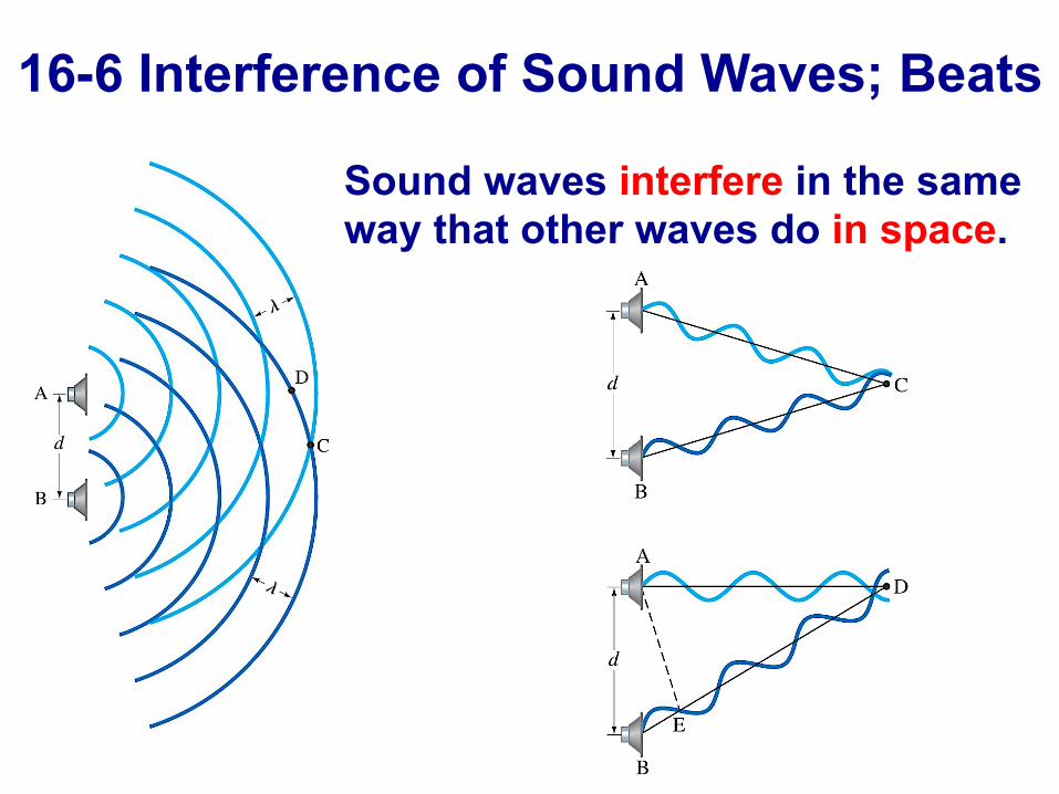
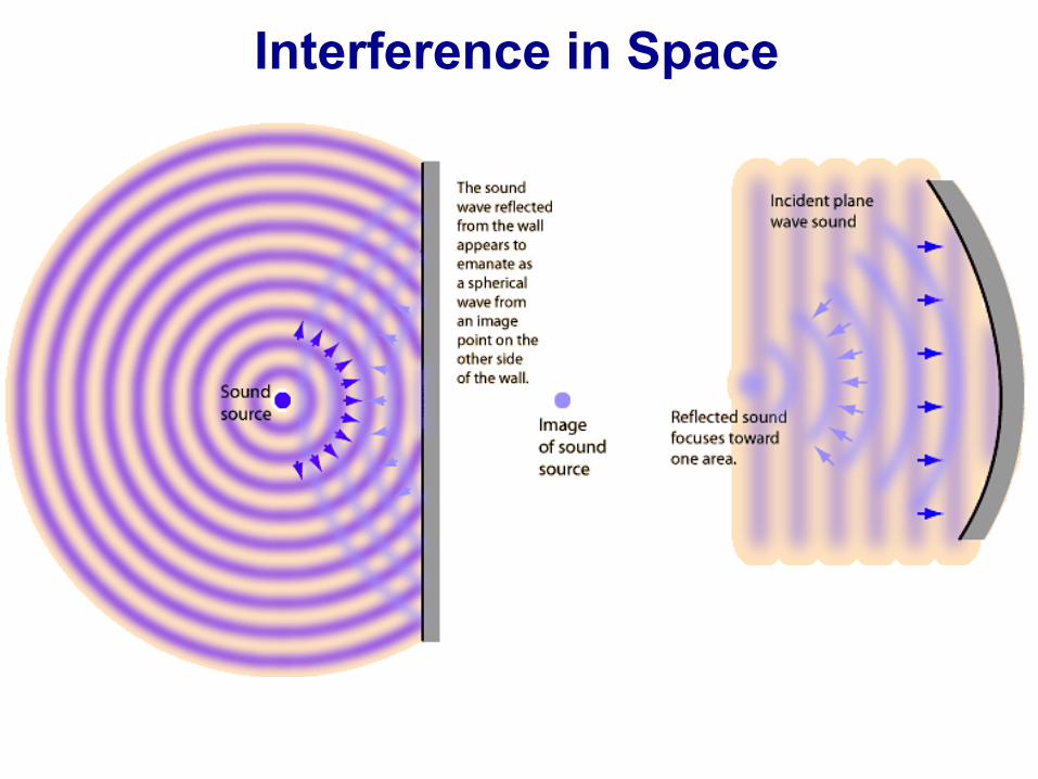
Sound waves interfere in the same way that other waves do in space.

16-6 Interference of Sound Waves; Beats

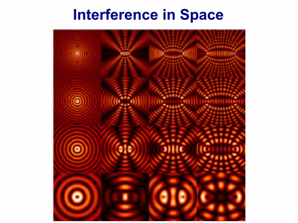
Interference in Space

Interference in Space

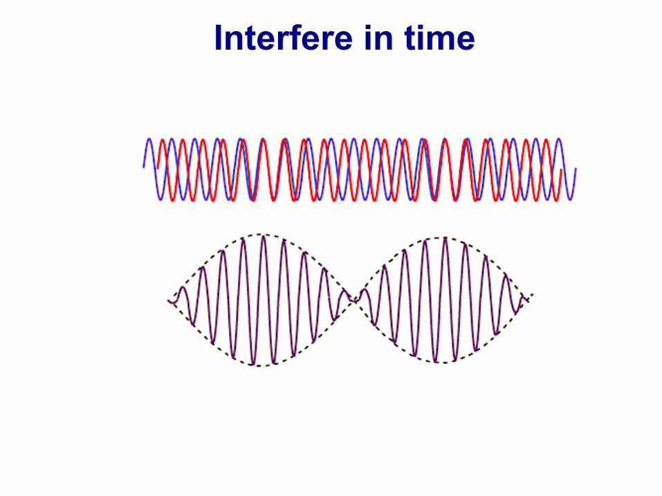
Interfere in time  

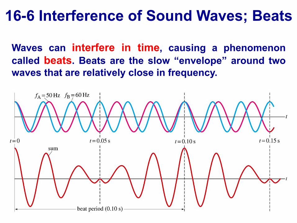
Waves can interfere in time, causing a phenomenon called beats. Beats are the slow “envelope” around two waves that are relatively close in frequency.

16-6 Interference of Sound Waves; Beats

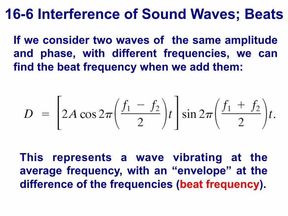
16-6 Interference of Sound Waves; Beats If we consider two waves of the same amplitude and phase, with different frequencies, we can find the beat frequency when we add them:

This represents a wave vibrating at the average frequency, with an “envelope” at the difference of the frequencies (beat frequency).

Experiment

Chapter 31

Maxwell’s Equations and Electromagnetic Waves

A short review

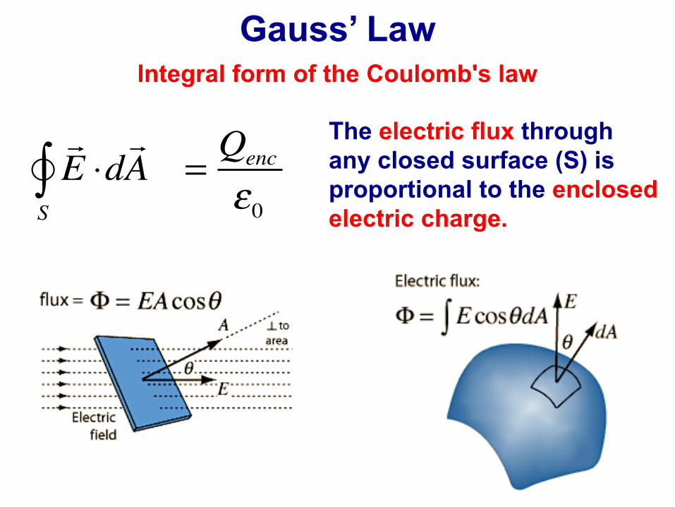
Gauss’ Law

E ⋅dA

S∫ =

Qenc

ε0

The electric flux through any closed surface (S) is proportional to the enclosed electric charge.

Integral form of the Coulomb's law

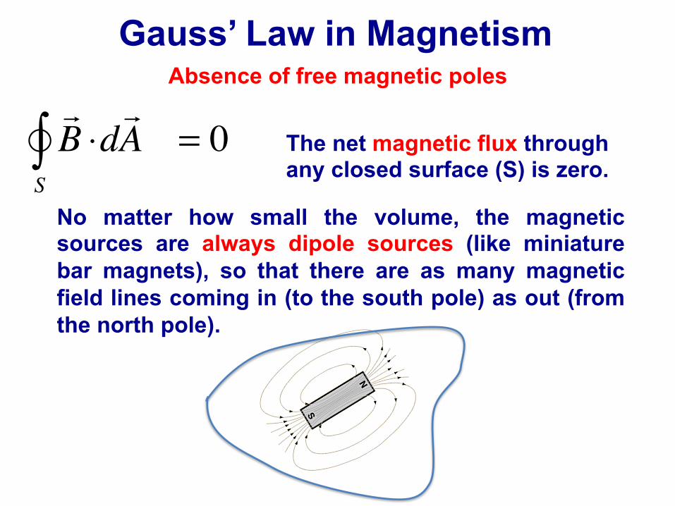
Absence of free magnetic poles Gauss’ Law in Magnetism

The net magnetic flux through any closed surface (S) is zero.

B ⋅dA

S∫ = 0

No matter how small the volume, the magnetic sources are always dipole sources (like miniature bar magnets), so that there are as many magnetic field lines coming in (to the south pole) as out (from the north pole).

E ⋅∫ dl = −

ddt

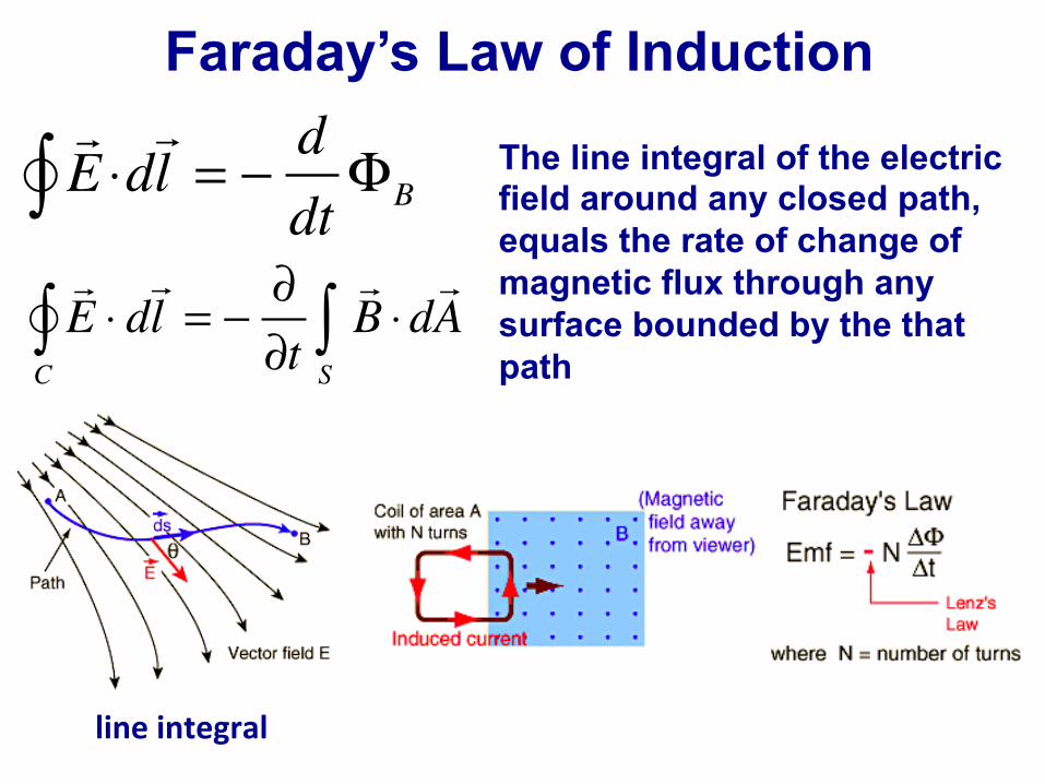
ΦBThe line integral of the electric field around any closed path, equals the rate of change of magnetic flux through any surface bounded by the that path

Faraday’s Law of Induction

line  integral    

E ⋅

C∫ d

l = −

∂∂t

B ⋅dA

S∫

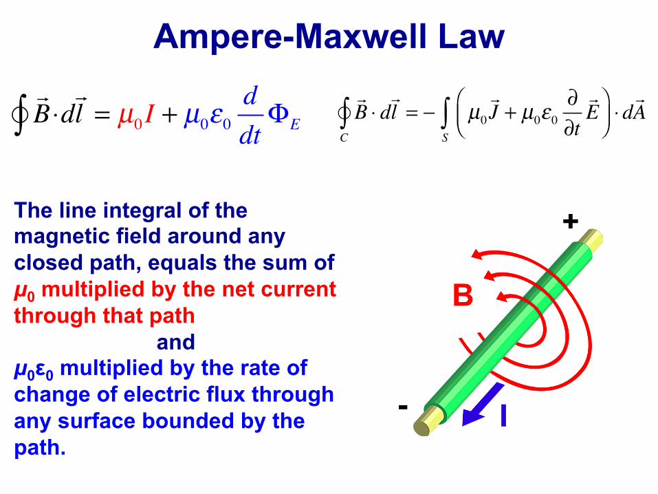
Ampere-Maxwell Law

B ⋅∫ dl = µ0I + µ0ε0

ddt

ΦE

The line integral of the magnetic field around any closed path, equals the sum of µ0 multiplied by the net current through that path

and µ0ε0 multiplied by the rate of change of electric flux through any surface bounded by the path.

B ⋅

C∫ d

l = − µ0

J + µ0ε0

∂∂tE⎛

⎝⎜⎞⎠⎟⋅dA

S∫

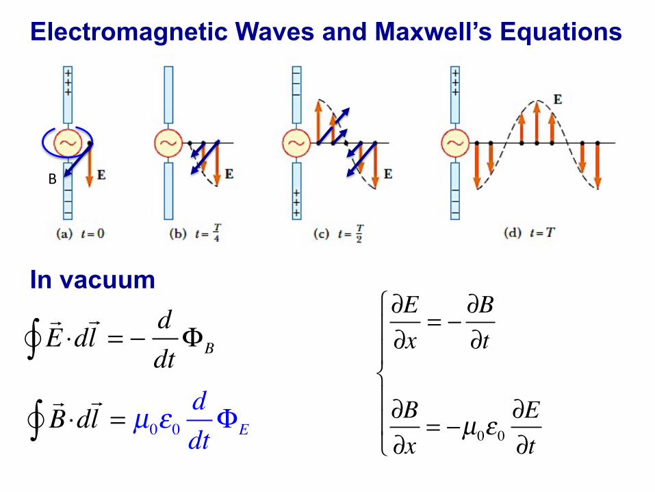
Electromagnetic Waves and Maxwell’s Equations

∂E∂x

= −∂B∂t

∂B∂x

= −µ0ε0∂E∂t

⎧

⎨

⎪⎪

⎩

⎪⎪

E ⋅∫ dl = −

ddt

ΦB

B ⋅∫ dl = µ0ε0

ddt

ΦE

In vacuum

B  

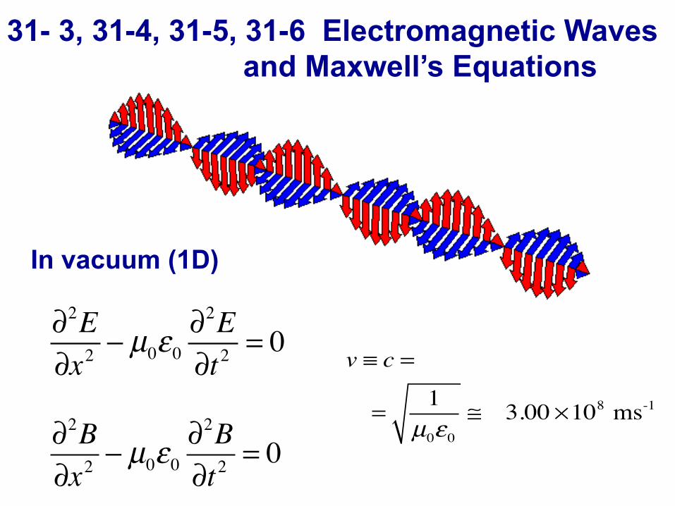
∂2E∂x2

− µ0ε0∂2E∂t2

= 0

In vacuum (1D)

31- 3, 31-4, 31-5, 31-6 Electromagnetic Waves and Maxwell’s Equations

∂2B∂x2

− µ0ε0∂2B∂t2

= 0

v ≡ c =

= 1µ0ε0

≅ 3.00 ×108 ms-1

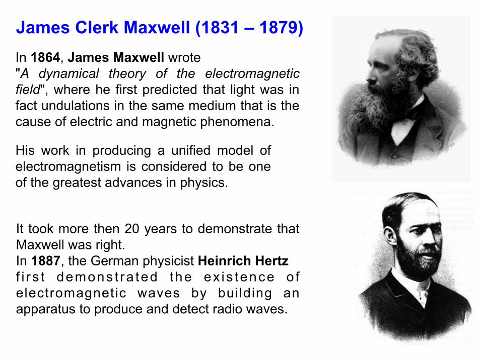
In 1864, James Maxwell wrote "A dynamical theory of the electromagnetic field", where he first predicted that light was in fact undulations in the same medium that is the cause of electric and magnetic phenomena.

James Clerk Maxwell (1831 – 1879)

His work in producing a unified model of electromagnetism is considered to be one of the greatest advances in physics.

It took more then 20 years to demonstrate that Maxwell was right. In 1887, the German physicist Heinrich Hertz f i r s t demons t ra ted the ex i s tence o f electromagnetic waves by building an apparatus to produce and detect radio waves.