Webb VESPA Manual - dfzljdn9uc3pi.cloudfront.net fileThe VESPA (Very large-scale Evolution and...

VESPA Manual

Version 1.0β

Andrew E. Webb, Thomas A. Walsh and Mary J. O’Connell

September, 2015

www.mol-evol.org/VESPA

2

Table of Contents

Table of Figures ......................................................................................................................... 3

1.1: Introduction ......................................................................................................................... 4

1.2: Phase and Pipeline Structure ............................................................................................... 5

1.3: Command Structure ............................................................................................................ 8

1.4: Basic and Required Options ............................................................................................... 9

1.5: VESPA Commands .......................................................................................................... 10

1.6: Phase One: Data Preparation ............................................................................................ 11

1.6.1: Clean Functions ............................................................................................................. 12

1.6.2: Translate Function ......................................................................................................... 14

1.6.3: Create Database Function .............................................................................................. 16

1.6.4: Gene Selection Function ................................................................................................ 18

1.6.5: Supplementary Functions .............................................................................................. 20

1.7: Phase Two: Homology Searching .................................................................................... 21

1.7.1: Core Options .................................................................................................................. 21

1.7.2: Similarity Group and Reciprocal Group Functions ....................................................... 22

1.7.3: Best-Reciprocal Similarity Group (Species-based) Function ........................................ 22

1.8: Phase Three: Alignment Assessment and Phylogeny Reconstruction .............................. 25

1.8.1: Alignment Comparison Function ................................................................................... 26

1.8.2: Empirical Model Selection Functions ............................................................................ 27

1.8.3: MrBayes Setup Function ............................................................................................... 28

1.9: Phase Four: Selection Analysis Preparation ..................................................................... 30

1.9.1: Alignment Mapping Function ........................................................................................ 31

1.9.2: Gene Tree Inference Function ....................................................................................... 33

1.9.3: CodeML Setup Function ................................................................................................ 35

1.9.4: MrBayes Reader Function ............................................................................................. 37

1.9.5: Subtree Function ............................................................................................................ 38

1.9.6: Create Branch Table Function ....................................................................................... 40

1.10: Phase Five: Selection Analysis Assessment ................................................................... 41

1.10.1: CodeML Results Assessment Function ....................................................................... 41

1.12: Third-Party Programs ..................................................................................................... 46

1.13: References ....................................................................................................................... 47

3

Table of Figures

Figure 1: Overview of the core functions within the VESPA toolkit. ....................................... 6

Figure 2: Overview of ‘clean’ and ‘clean_ensembl’ functions. ............................................... 13

Figure 3: Overview of ‘translate’ function. ............................................................................. 15

Figure 4: Overview of ‘create_database’ function. .................................................................. 17

Figure 5: Overview of ‘gene_selection’ function. ................................................................... 19

Figure 7: Overview of ‘mrbayes_setup function. .................................................................... 29

Figure 8: Overview of the ‘map_alignments’ function ............................................................ 32

Figure 9: Overview of the ‘infer_genetree’ function. .............................................................. 34

Figure 10: Overview of the ‘codeml_setup’ function. ............................................................. 36

Figure 11: Overview of the ‘create_subtrees’ function. .......................................................... 39

Figure 12: Sample supplementary output file created by ‘codeml_reader’ ............................. 42

Figure 13: Sample specialized MSA created by ‘codeml_reader’ ........................................... 44

4

1.1: Introduction

The VESPA (Very large-scale Evolution and Selective Pressure analyses) toolkit is a collection of commands designed to simplify molecular evolutionary analyses. The major motivation behind the development of VESPA was minimizing potential sources of error in large-scale selective pressure analyses using codeML from the PAML package [Yang 2007].

Assessing selective pressure variation on a large scale using protein coding DNA sequences requires a complex pipeline composed of numerous independent analyses, including: ortholog identification, multiple sequence alignment, phylogenetic reconstruction, and assessment of codon-based models of evolution. The pipeline requires multiple data manipulation steps to combine the output of each of these different stages (such as parsing BLAST result files to identify homologs and assessment of the suitability of the phylogenetic tree for selective pressure analysis). For researchers new to bioinformatics, manual data manipulation is prone to error, is potentially unstandardized, and is difficult to reproduce. VESPA eliminates the need for manual data manipulation by creating functions that automatically complete the majority of data manipulation steps using a standardized approach. In addition, the use of VESPA should minimize the requirements for users to create their own programs.

While the procedures within each stage of a selective pressure analysis are independent, there are requirements on the order in which the phases are carried out. VESPA creates a standardize pipeline of analyses with a specific ordering of phases in the process. In addition, the package encompasses multiple specialized pipelines to accurately assess selective pressure and reduce potential false positives (such as those caused by alignment error [Fletcher and Yang, 2010]).

Lastly, VESPA was designed to increase user productivity by automating labor intensive or highly repetitive tasks: i) automation by recursion – used to repeat an analysis on a number of files (e.g. cleaning and translating a directory of genomes), and ii) automation of analysis methods – used to complete tasks that are normally demanding but invariable in execution (e.g. identifying homologs within BLAST output data). Automating these procedures within VESPA has created an analysis package that is highly scalable (i.e. from single gene to whole genome analyses) and that flexible enough to be useful for many levels of expertise and many alternative purposes/endpoints.

5

1.2: Phase and Pipeline Structure

The VESPA toolkit is separated into five separate analysis phases (Figure 1). The rationale behind the “phase” system was primarily to aid users in understanding the distinct procedures involved in selective pressure analysis and to provide more advanced users with a flexible and adaptable pipeline. Functions within a phase also analyze the same input type (e.g. sequences, BLAST output, etc.).

The output of each phase in the VESPA toolit requires an analysis step that must be completed by the user with third-party software (Figure 1). These analyses are not automated by VESPA for three reasons: i) these analyses are far too computationally intensive, and ii) the submission process for these programs may differ from user to user, and iii) software updates may create bugs within the pipeline.

The software package also incorporates two analysis pipelines, a basic pipeline for single gene orthologs (SGOs) and an advanced pipeline for both SGOs and multi-gene families (MGFs). The basic pipeline was designed to bypass the phylogenetic reconstruction techniques (phase 3) by inferring a gene phylogeny from a user-defined species phylogeny. Usage of the basic pipeline is only recommended if the genes are confirmed SGOs. See Figure 1 for additional details on the pipelines.

6

Figure 1: Overview of the core functions within the VESPA toolkit.

Translate

orEnsembl Clean Clean

Database

Gene SelectionorP

hase 1

BLAST or HMMER

Best Reciprocal Groups

or

Similarity Groups

Reciprocal Groups

or

Identify SGOs

Sequence Alignment

Ph

ase 2

CodeML Analysis

Ph

ase 4 Infer Gene Trees

CodeML Setup

Map Alignments

Branch-site Setupor

MrBayes Reader

CodeML Setup

Branch-site Setupor

Create Sub-Treesor

Phylogenetic Reconstruction

Ph

ase 3

ProtTest Reader

MrBayes Setup

ProtTest Setup

metAl Compare or or

Model Selection

metAl Compare

Basic

SG

O

Analy

sis

Basic

SG

O

Analy

sis

or

Ph

ase 5

CodeML ReaderCodeML

Alignments

CodeML Reader

CodeML

Alignments

a

b

c

d

e

7

Figure 1 Legend Each phase indicates the functions (white boxes) and the order in which they are invoked. Optional functions are indicated by ‘or’ and may be skipped. Dark boxes indicate third-party programs. (a) Phase 1 (Section 1.6) is the data preparation phase and includes the functions: ensembl_clean/clean (Section 1.6.1), translate (Section 1.6.2), create_database (Section 1.6.3), and gene_selection (Section 1.6.4). This phase ends with the requirements for sequence similarity searching. (b) Phase 2 (Section 1.7) is the similarity group creation phase and includes the following functions: similarity_groups (Section 1.7.2), reciprocal_groups (Section 1.7.2) and best_reciprocal_groups (Section 1.7.3). This phase results in the creation of requirements for multiple sequence alignment (MSA). (c) Phase three (Section 1.8) is the alignment assessment stage and includes both a basic pipeline (on the left) for MSA files that contain only single gene orthologous (SGOs) and an advanced pipeline (on the right) for unconfirmed MSA files. The phase includes the following functions: metal_compare (Section 1.8.1), protest_setup (Section 1.8.2), protest_reader (Section 1.8.2), and mrbayes_setup (Section 1.8.3). This phase results in either: i) a phylogenetic trees of the MSAs for the advanced pipeline or ii) selected MSAs for the basic pipeline. (d) Phase four (Section 1.9) is the selective pressure phase and continues the basic pipeline and advanced pipeline of the previous phase. The phase four basic pipeline includes: map_alignment (Section 1.9.1), infer_genetree (Section 1.9.2), setup_codeml (Section 1.9.3), and create_branch (Section 1.9.6). The phase four advanced pipeline includes: mrbayes_reader (Section 1.9.4), create_subtrees (Section 1.9.5), create_branch (Section 1.9.6), and setup_codeml (Section 1.9.3). This phase results in the input requirements for selective pressure analysis by codeML. (e) The final phase (Section 1.10) includes the function codeml_reader (Section 1.10.1) that analyzes the results of the codeML analysis.

8

1.3: Command Structure

The VESPA software package was written in python (v2.7) and requires a UNIX environment to operate. VESPA may be invoked as follows:

usr$ python vespa.py

The VESPA help screen will then be displayed by default. If desired, the help screen may also be displayed using the following commands.

usr$ python vespa.py help

usr$ python vespa.py h

In addition to the basic help screen, VESPA has the option to display basic help information for each VESPA command. If desired, the help information may be displayed by specifying the command of interest subsequent to the help screen call (please note the space):

usr$ python vespa.py help translate

Commands in VESPA are specified after the program call (i.e. python vespa.py) on the UNIX command-line. Please note a space is required between the program call and the desired command. For example, the translate command would be invoked as shown below:

usr$ python vespa.py translate

Commands also require specific options to be invoked to function correctly. Options are specified after the command and begin with a dash symbol (-) and end with an equal sign (=) followed by either a user-specified file or Boolean value (i.e. True/False). For example, the translate command requires the user to specify the input (here “user_data.txt”) as follows:

usr$ python vespa.py translate -input=user_data.txt

Please note the space between the command and option, it should also be noted that there is no space separating the option (i.e. “-input=”) and the user-specification (i.e. “user_data.txt”). Multiple options may be invoked on the same command-line as shown below and are separated by a space:

usr$ python vespa.py translate -input=user_data.txt -cleave_terminal=False

A comprehensive list of the commands supported in VESPA may be found on Pg. 10 of this manual.

9

1.4: Basic and Required Options

Commands in VESPA (see this manual Pg. 10) use two categories of options: basic and command-specific. Basic options may be invoked alongside any command, whereas command-specific options are limited to particular commands. This version of VESPA incorporates two basic options: ‘input’ and ‘output’.

The ‘input’ option: This option is invoked by the user to indicate the desired input file or directory for a command. As indicated, this option is designed to function with either: i) an individual file or ii) a directory housing multiple files. Please note that the ‘input’ option is a REQUIRED option and therefore is required by all commands to function. Not specifying the input option will result in VESPA printing a warning message. Please note that ‘USR_INPUT’ is a placeholder for the input defined by the user.

usr$ python vespa.py temp_command -input=USR_INPUT

For example, if a user wanted to analyze the directory “Genomes” they would type:

usr$ python vespa.py temp_command -input=Genomes

The ‘output option: This option indicates the desired name the user supplies for the output of a command. Depending on the input used, the option will either specify: i) the output filename (if an individual file was the input), or ii) the output directory name (if a directory was the input). It should be noted that some commands have specialized output, in these cases the desired name will be applied where possible.

usr$ python vespa.py command -input=USR_INPUT –output=USR_DEF

10

1.5: VESPA Commands

Phase One Phase Two Phase Three Phase Four Phase Fiveclean similarity_groups metal_compare map_alignments codeml_readerclean_ensembl reciprocal_groups prottest_setup infer_genetreerev_complement best_reciprocal_groups prottest_reader mrbayes_readertranslate mrbayes_setup codeml_setupcreate_database create_subtreesgene_selection create_branchindividual_sequencessplit_sequences

11

1.6: Phase One: Data Preparation

The data preparation phase was included for users new to bioinformatics. The phase prepares downloaded genomes for homology searching using the two VESPA supported homology search tools: BLAST [Altschul et al., 1990] and HMMER [Eddy, 1998]. This phase also includes supplementary functions not required for either pipeline shown in Figure 1 but rather to aid users in homology searching.

12

1.6.1: Clean Functions

The VESPA toolkit incorporates two quality control (QC) functions: ‘clean’ and ‘clean_ensembl’.

The ‘clean’ function: This basic function was designed as a QC filter for downloaded nucleotide sequences and/or genomes (Figure 2a). Each sequence is confirmed as protein coding by using a conditional statement to verify that the nucleotide sequence contains only complete codons (i.e. the length of the sequence is exactly divisible by 3) (Figure 2b). This is an essential step to confirm gene annotation quality and permit the codon substitution models of codeML [Yang, 2007]. Only sequences that pass QC are retained for further analysis (Figure 2c).

usr$ python vespa.py clean –input=USR_INPUT

The ‘clean_ensembl’ function: This more advanced function was designed to identify the longest nucleotide (canonical) transcript within an Ensembl nucleotide genome that passed the QC step detailed in the ‘clean’ function. This is achieved by exploiting the pattern of ensembl sequence identifiers, which consistently begin with the gene identifier followed by the transcript identifier (Figure 2d). The longest transcript is then identified for each ensembl gene identifier and saved within the output file.

usr$ python vespa.py clean_ensembl –input=USR_INPUT

Supported file format(s): ‘input’: fasta formatted files

Command-specific options: Both clean functions incorporate a single enabled option (‘rm_internal_stop’) and two disabled options (‘label_filename’ and infer_ensembl_species’) that may be manually configured by the user. The option ‘rm_internal_stop’ will remove sequences if they contain an internal stop codon (Figure 2g), those removed will be reported in the command log file. It should be noted that while ‘rm_internal_stop’ is configurable, codeML does not permit nonsense mutations and this option should be enabled if the toolkit is being used for that purpose. The options ‘label_filename’ and ‘infer_ensembl_species’ alter sequence headers (i.e. Ensembl gene and transcript identifiers) by adding an additional identifier at the beginning of the header: ‘infer_ensembl_species’ adds the common species name of the respective Ensembl identifier (Figure 2e) and ‘label_filename’ adds the filename (without the file extension) (Figure 2f). It should be noted that executing a labeling option is required for enabling VESPA to automate the creation of gene trees and setup of the codeML branch-site models (for details see Section 1.9.6).

usr$ python vespa.py clean –input=USR_INPUT -rm_internal_stop=False

usr$ python vespa.py clean –input=USR_INPUT -label_filename=True

usr$ python vespa.py clean –input=USR_INPUT -infer_ensembl_species=True

13

Figure 2: Overview of ‘clean’ and ‘clean_ensembl’ functions.

Figure 2 Legend FastA formatted files are shown as grey boxes and the associated white boxes show the filename. Data confirmation steps shown as readout beneath each example indicates if the results passed the check. The following QC checks are illustrated here: (a) Cleaning an input file, (b) initiates with codon confirmation, (c) only sequences that pass are saved in the output. If the ‘ensembl_clean’ function is invoked, in addition to codon confirmation, each transcript of an ensembl gene undergoes (d) a longest transcript confirmation and only the longest transcript is saved in the output. Two options are available to append a prefix to sequence headers: (e) ‘infer_ensembl_species’ to append the Ensembl genome, or (f) ‘label_filename’ to append the input filename. Invoking (g) ‘rm_internal_stop’ will remove genes that fail stop codon confirmation.

>ENSG00000003137|ENST00000001146|1539ATGCTCTTTGAGGGCTTGGATCTGGTGTCGGCGCTGGCCACCCTCGCCGCGTGCCTGGTG...TAG>ENSG00000001630|ENST00000003100|1530ATGGCGGCGGCGGCTGGGATGCTGCTGCTGGGCTTGCTGCAGGCGGGTGGGTCGGTGCTG...TAG>ENSG00000170469|ENST00000302091|881ATGGCGACGCCCCTCGGGTGGTCGAAGGCGGGGTCAGGATCTGTGTGTCTCGCTTTAGAT...TA

Human.fasta

Pass: ATG - CTC - TTT - GAG - GGC - TTG - GAT - ··· - TAGFail: ATG - CTC - TTT - GAG - GGC - TTG - GAT - ··· - TA_

Pass: ENSG00000003137|ENST00000001146 – Seq length: 930Fail: ENSG00000003137|ENST00000546307 – Seq length: 900Fail: ENSG00000003137|ENST00000412253 – Seq length: 600

>ENSG00000003137|ENST00000001146|1539ATGCTCTTTGAGGGCTTGGATCTGGTGTCGGCGCTGGCCACCCTCGCCGCGTGCCTGGTG...TAG>ENSG00000001630|ENST00000003100|1530ATGGCGGCGGCGGCTGGGATGCTGCTGCTGGGCTTGCTGCAGGCGGGTGGGTCGGTGCTG...TAG

Cleaned_Human.fasta

a

b

c

d

>ENSG00000003137|ENST00000001146|1539ATGCTCTTTGAGGGCTTGGATCTGGTGTCGGCGCTGGCCACCCTCGCCGCGTGCCTGGTG...TAG

Human.fasta

>Human|ENSG00000003137|ENST00000001146|1539ATGCTCTTTGAGGGCTTGGATCTGGTGTCGGCGCTGGCCACCCTCGCCGCGTGCCTGGTG...TAG

Output

>CYP26B1ATGCTCTTTGAGGGCTTGGATCTGGTGTCGGCGCTGGCCACCCTCGCCGCGTGCCTGGTG...TAG

Human.fasta

>Human|CYP26B1ATGCTCTTTGAGGGCTTGGATCTGGTGTCGGCGCTGGCCACCCTCGCCGCGTGCCTGGTG...TAG

Output

e

f

gFail:

ATG - CTC - TTT - GAG - GGC - TTG - GAT - ··· - TAGM L F E G L D · *Pass:

ATG - CTC - TTT - TAG - GGC - TTG - GAT - ··· - TAGM L F * G L D · *

14

1.6.2: Translate Function

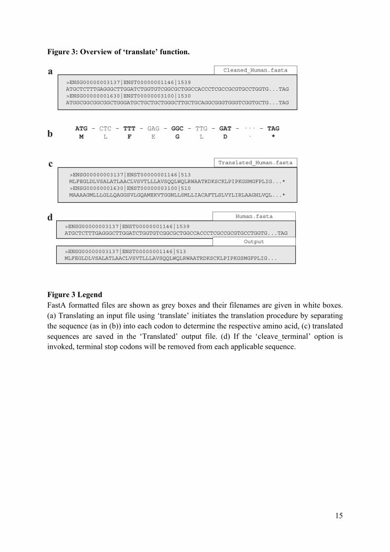
The ‘translate’ function translates nucleotide sequences that passed the QC filter of either clean function into amino acid sequences in the first reading frame forward only (Figure 3a). The function operates by splitting the nucleotide sequence into codons and then translating them into their respective amino acids (Figure 3b). Translation is a mandatory step to produce alignments permitted by the codon substitution models of codeML (see Section 1.9.1) [Yang, 2007]. The resulting protein sequences are then saved (Figure 3c). If non-coding sequences (incomplete codons or internal stop codons) were not removed prior to invoking the ‘translate’ function, the function will produce a warning message. The warning reports that the function is designed to only translate protein-coding sequences and terminates the function.

usr$ python vespa.py translate –input=USR_INPUT

Command-specific options: The ‘translate’ function incorporates a single unique option ‘cleave_terminal’ and the previously described options of the clean functions (Section 1.6.1). The ‘cleave_terminal’ option is enabled by default and is designed to cleave the terminal stop codon of each sequence (Figure 3d). The function and default status of the remaining options are detailed in Section 1.6.1.

usr$ python vespa.py translate –input=USR_INPUT -cleave_terminal=False


15

Figure 3: Overview of ‘translate’ function.

Figure 3 Legend FastA formatted files are shown as grey boxes and their filenames are given in white boxes. (a) Translating an input file using ‘translate’ initiates the translation procedure by separating the sequence (as in (b)) into each codon to determine the respective amino acid, (c) translated sequences are saved in the ‘Translated’ output file. (d) If the ‘cleave_terminal’ option is invoked, terminal stop codons will be removed from each applicable sequence.

ATG - CTC - TTT - GAG - GGC - TTG - GAT - ··· - TAGM L F E G L D · *

>ENSG00000003137|ENST00000001146|513MLFEGLDLVSALATLAACLVSVTLLLAVSQQLWQLRWAATRDKSCKLPIPKGSMGFPLIG...*>ENSG00000001630|ENST00000003100|510MAAAAGMLLLGLLQAGGSVLGQAMEKVTGGNLLSMLLIACAFTLSLVYLIRLAAGHLVQL...*

Translated_Human.fasta

>ENSG00000003137|ENST00000001146|1539ATGCTCTTTGAGGGCTTGGATCTGGTGTCGGCGCTGGCCACCCTCGCCGCGTGCCTGGTG...TAG>ENSG00000001630|ENST00000003100|1530ATGGCGGCGGCGGCTGGGATGCTGCTGCTGGGCTTGCTGCAGGCGGGTGGGTCGGTGCTG...TAG

Cleaned_Human.fastaa

b

c


Human.fasta

>ENSG00000003137|ENST00000001146|513MLFEGLDLVSALATLAACLVSVTLLLAVSQQLWQLRWAATRDKSCKLPIPKGSMGFPLIG...

Output

d

16

1.6.3: Create Database Function

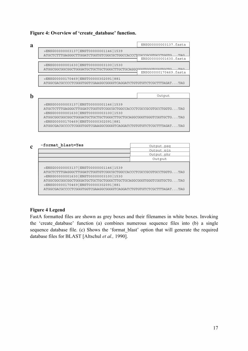
The ‘create_database’ function was designed for users to concatenate multiple genomes into the single database required for homology searching. The function operates by building the database a single sequence at a time (Figure 4a and b). The command-line version of BLAST requires additional commands to create a BLAST-formatted database. If the user enables the option ‘format_blast’ and BLAST is installed on the system the function will attempt to automate the additional steps required for producing a BLAST-ready database (Figure 4c). If ‘create_database’ is unable to create the BLAST-formatted database, a warning message will be produced (see Section 1.12 BLAST version requirements).

usr$ python vespa.py create_database –input=USR_INPUT


17

Figure 4: Overview of ‘create_database’ function.

Figure 4 Legend FastA formatted files are shown as grey boxes and their filenames in white boxes. Invoking the ‘create_database’ function (a) combines numerous sequence files into (b) a single sequence database file. (c) Shows the ‘format_blast’ option that will generate the required database files for BLAST [Altschul et al., 1990].

ENSG00000003137.fasta



>ENSG00000001630|ENST00000003100|1530ATGGCGGCGGCGGCTGGGATGCTGCTGCTGGGCTTGCTGCAGGCGGGTGGGTCGGTGCTG...TAG

>ENSG00000170469|ENST00000302091|881ATGGCGACGCCCCTCGGGTGGTCGAAGGCGGGGTCAGGATCTGTGTGTCTCGCTTTAGAT...TAG


a

>ENSG00000003137|ENST00000001146|1539ATGCTCTTTGAGGGCTTGGATCTGGTGTCGGCGCTGGCCACCCTCGCCGCGTGCCTGGTG...TAG>ENSG00000001630|ENST00000003100|1530ATGGCGGCGGCGGCTGGGATGCTGCTGCTGGGCTTGCTGCAGGCGGGTGGGTCGGTGCTG...TAG>ENSG00000170469|ENST00000302091|881ATGGCGACGCCCCTCGGGTGGTCGAAGGCGGGGTCAGGATCTGTGTGTCTCGCTTTAGAT...TAG

Outputb

c Output.psqOutput.pinOutput.phr

-format_blast=Yes


Output

18

1.6.4: Gene Selection Function

If the user is only interested in a subset of genes, the ‘gene_selection’ function was designed to enable the user to search a database for gene identifiers specified in a separate file. The function operates by searching the sequence headers of the database for matches with the user specified gene identifiers (Figure 5a). The matching process only requires the user-specified identifiers to match a portion of the database sequence headers (Figure 5b). The function saves a single sequence file for each matched identifier (Figure 5c). If a user-specified identifier matches more than a single sequence header in the database, or indeed no sequence in the database, the function will produce a warning message. It should be noted that the ‘gene_selection’ function requires the option ‘selection_csv’ to operate.

usr$ python vespa.py gene_selection –input=USR_INPUT -selection_csv=USR_INPUT

Supported file format(s): ‘input’: fasta formatted files; ‘selection_csv’: csv, tsv, and unformatted.

19

Figure 5: Overview of ‘gene_selection’ function.

Figure 5 Legend FastA formatted files are shown as grey boxes and their filenames in white boxes. Data confirmation steps indicate if the results passed the check. (a) The ‘gene_selection’ function requires two files to operate: a database (Human.fasta) and a user specified gene identifiers file (genes.csv). (b) The function operates using header confirmation to identify sequences in the database that match to those specified by the user. (c) The output of the function is a single sequence file for each user specified genes found.


Human.fasta

ENSG00000003137ENSG00000001630

genes.csv




>ENSG00000001630|ENST00000003100|1530ATGGCGGCGGCGGCTGGGATGCTGCTGCTGGGCTTGCTGCAGGCGGGTGGGTCGGTGCTG...TAG

a

c

Pass: ENSG00000003137 >ENSG00000003137|ENST00000001146Pass: ENSG00000001630 >ENSG00000001630|ENST00000003100Fail: >ENSG00000170469|ENST00000302091

b

20

1.6.5: Supplementary Functions

The VESPA toolkit also incorporates three supplementary functions that were designed to aid users in potential data manipulations required for homology searching: ‘rev_complement’, ‘individual_sequences’, and ‘split_sequences’.

The ‘rev_complement’ function: This function was designed for users to return the reverse complement of nucleotide sequences. Depending on the desired use, it is recommended that the user run the QC filter of the clean functions either preceding or proceeding the ‘rev_complement’ function.

usr$ python vespa.py rev_complement –input=USR_INPUT


Command-specific options: The ‘rev_complement’ function incorporates the two labeling options of the clean functions (previously described in Section 1.6.1). It should be noted that the option ‘rm_internal_stop’ was not included in this function.

The ‘individual_sequences’ function: This function was designed for users to separate files/directories housing large collections of sequences (i.e. genome file(s) and database files) into individual sequence files.

usr$ python vespa.py individual_sequences –input=USR_INPUT


The ‘split_sequences’ function: This function was designed for users to separate files/ directories housing large collections of sequences (i.e. genome file(s) and database files) into sequence files that house a specified number of sequences. The number of sequences in each output file may be specified using the ‘split_number’ option; otherwise the default value of 100 is used.

usr$ python vespa.py split_sequences –input=USR_INPUT –split_number=USR_DEF


21

1.7: Phase Two: Homology Searching

The second phase of VESPA is concerned with identifying groups of similar sequences from either BLAST [Altschul et al., 1990] or HMMER [Eddy, 1998] homology searches. Three types of sequence similarity are recognized by VESPA: non-reciprocal (unidirectional), reciprocal (bidirectional), and best-reciprocal. “Non-reciprocal similarity” is characterized by sequence similarity that is only detected by one of the pair of sequences, commonly resultant of an E-value near the threshold. Non-reciprocal similarity is generally distantly related sequences. “Reciprocal similarity” is similarity identified by both sequences in the pair. Reciprocal similarity is typically closely related orthologs or paralogs. “Best-reciprocal similarity” requires that the sequences pass two criteria: (i) they are sequences from different species, and (ii) in the pair-wise connection each sequence finds no other sequence in the respective species with a lower E-value. These requirements limit identification to orthologs (non-orthologs may be identified due to identical E-values or the absence of a true ortholog).

Each type of similarity connection is invoked using a separate function and will generate the families specific to that connection type. Each function is required to be linked to a protein sequence database (Section 1.6.3). The database is used to produce an output file of each similarity group containing the protein sequences of each member. Each protein sequence files then undergoes multiple sequence alignment.

1.7.1: Core Options

The ‘input’ option of each function within the second phase is designed to accept the modular output of BLAST and the standard output of HMMER (i.e. USR_HOMOLOGY). In addition, each function also requires both the ‘database’ and ‘format’ options. The ‘database’ option is used to specify the protein sequence database created by earlier in the VESPA pipeline (i.e. ‘USR_DB’) (Section 1.6.3) whereas the ‘format’ option is used to specify the input format as either ‘blast’ or ‘hmmer’. Please note that commands below are written on a single line.

usr$ python vespa.py similarity_groups –input=USR_HOMOLOGY –format=blast –database=USR_DB

Each function also includes three optional threshold options that are disabled by default: ‘e_value’, ‘alignment_length’, and ‘percent_identity’. The three options enable the user to define threshold values for the E-value, alignment length, and percentage identity of each homology connection. Enabled thresholds must be passed for a pair-wise homology connection to be used in creating similarity groups. If an E-value threshold is not enabled, each function is designed to only accept E-values < 1, otherwise warning message is printed.

usr$ python vespa.py similarity_groups –input=USR_HOMOLOGY –format=blast -database=USR_DB -e_value=0.001

usr$ python vespa.py similarity_groups –input=USR_HOMOLOGY –format=blast -database=USR_DB -alignment_length=75

usr$ python vespa.py similarity_groups –input=USR_HOMOLOGY –format=blast -database=USR_DB -percent_identity=75

22

1.7.2: Similarity Group and Reciprocal Group Functions

The ‘similarity_groups’ and ‘reciprocal_groups’ functions both construct sequence similarity groups using a similar approach. Both functions iteratively read a single line of input (BLAST or HMMER output) and record only the name of the query and subject if they pass enabled thresholds. Limiting the recorded data of the homology search to sequence names and their respective role (query or subject) results in reduced computational requirements, increased function speed, and permits the function to parse larger BLAST or HMMER input files. Both functions are able to recognize and record input that denotes reciprocal homology of a previously recorded entry. Once each function has completed processing the input, the pair-wise homologs are used to build families. The ‘similarity_groups’ function allows both non-reciprocal and reciprocal connections within a sequence group (Figure 6a) whereas ‘reciprocal_groups’ is restricted to reciprocal connection within a sequence group (Figure 6b).

usr$ python vespa.py similarity_groups –input=USR_HOMOLOGY –format=blast -database=USR_DB

usr$ python vespa.py reciprocal_groups –input=USR_HOMOLOGY –format=blast -database=USR_DB

Supported file format(s): ‘input’: BLAST tabular output format and HMMER standard output.

1.7.3: Best-Reciprocal Similarity Group (Species-based) Function

The ‘best_reciprocal_groups’ function constructs sequence homology groups by iteratively reading each line of input and storing the record within a database in reference to the query sequence. Once the function has completed parsing the input, the database is used to determine the best-homolog for each query sequence. This is achieved by identifying which subject sequence has the best E-value for each designated species. The designated best-hit for each query are then parsed to determine if the relationship is reciprocal (i.e. the subject sequence [as a query] identifies the query [as a subject]). If a query and subject are identified as best-reciprocal homology hits, they are used to create families (Figure 6c).

usr$ python vespa.py best_reciprocal_groups –input=USR_HOMOLOGY –format=blast -database=USR_DB

Supported file format(s): ‘input’: BLAST tabular output format and HMMER standard output.

23

Figure 6: Similarity groups created by functions

hGX

mGX

rGX

gGX

rGY

mGY

gGX2

hGX2

hGX

mGX

rGX

gGX

rGY

mGY

gGX2

hGX2

hGX

mGX

rGX

gGX

rGY

mGY

gGX2

hGX2

a

b

c

24

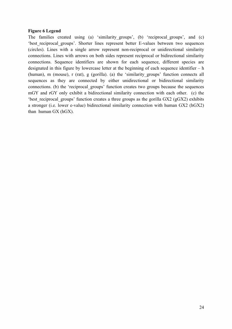
Figure 6 Legend The families created using (a) ‘similarity_groups’, (b) ‘reciprocal_groups’, and (c) ‘best_reciprocal_groups’. Shorter lines represent better E-values between two sequences (circles). Lines with a single arrow represent non-reciprocal or unidirectional similarity connections. Lines with arrows on both sides represent reciprocal or bidirectional similarity connections. Sequence identifiers are shown for each sequence, different species are designated in this figure by lowercase letter at the beginning of each sequence identifier – h (human), m (mouse), r (rat), g (gorilla). (a) the ‘similarity_groups’ function connects all sequences as they are connected by either unidirectional or bidirectional similarity connections. (b) the ‘reciprocal_groups’ function creates two groups because the sequences mGY and rGY only exhibit a bidirectional similarity connection with each other. (c) the ‘best_reciprocal_groups’ function creates a three groups as the gorilla GX2 (gGX2) exhibits a stronger (i.e. lower e-value) bidirectional similarity connection with human GX2 (hGX2) than human GX (hGX).

25

1.8: Phase Three: Alignment Assessment and Phylogeny Reconstruction

The third phase of VESPA combines multiple third-party programs (i.e. MetAl [Blackburne and Whelan, 2012] and NoRMD [Thompson et al., 2001]) to automate the assessment and choice of protein Multiple Sequence Alignments (MSAs). In addition this phase enables simplified large-scale phylogenetic reconstruction. Alignment error is reported to cause high rates of false positives in a selective pressure analysis [Fletcher and Yang, 2010]. Therefore, VESPA incorporates third-party programs for MSA comparison and scoring. A complete analysis of the MSAs from each method is recommended. The next step in this phase is the selection of the empirical model of evolution that best-fits each MSA [Darriba et al., 2011; Keane et al., 2006]. The third phase concludes with an automated method for generating the files necessary for phylogenetic reconstruction using the previously selected MSA and model of evolution. The functions of this phase are primarily designed to interface with selected third-party programs. However, each step of this phase has been made optional if the user has other preferences or needs.

26

1.8.1: Alignment Comparison Function

The ‘metal_compare’ function is designed to fully automate MSA comparison and scoring. The function operates using the third-party program MetAl [Blackburne and Whelan, 2012] to compare two protein MSAs. If MetAl indicates that the two MSAs are dissimilar, the function employs the third-party program noRMD [Thompson et al., 2001] to score each protein MSA using column-based similarity. The MSA with the highest noRMD (i.e. column-based similarity) score is then selected for subsequent analysis. It should be noted that the ‘metal_compare’ function requires the option ‘compare’ to operate.

usr$ python vespa.py metal_compare –input=USR_INPUT -compare=USR_INPUT

Command-specific options: The ‘metal_compare’ function incorporates one additional option (‘metal_cutoff’) that may be configured by the user. The ‘metal_cutoff’ option assigns the numeric threshold determining MSA dissimilarity and by default is fixed at 5%. Alignment methods that yield MetAl scores lower than defined value are considered comparable and the function will select the MSA from the first alignment method (indicated using the ‘input’ option).

usr$ python vespa.py metal_compare –input=USR_INPUT -compare=USR_INPUT - metal_cutoff=0.10

Supported file format(s): ‘input’ and ‘compare’: fasta formatted files (nexus and phylip formats to be added in version 0.3β).

27

1.8.2: Empirical Model Selection Functions

The ‘prottest_setup’ function: This function is designed to automate the process of identifying the best-fit model of amino acid replacement for a specified protein alignment using the third-party program ProtTest3 [Darriba et al., 2011]. The function is designed to test each amino acid substitution model in both the absence and presence of invariant sites, gamma categories, and a combination of the two.

usr$ python vespa.py prottest_setup –input=USR_INPUT

Supported file format(s): ‘input’: fasta formatted files (nexus and phylip formats to be added in version 0.3β).

The ‘prottest_reader’ function: This function automates the process of reading the output of ProtTest3. The function creates two output files: best_models.csv and best_supported_models.csv. The best models file reports the best-fit model of amino acid replacement (± rate-heterogeneity) reported by ProtTest3 whereas the best supported file reports the best-fit model of amino acid replacement (± rate-heterogeneity) supported by the third-party phylogenetic reconstruction program MrBayes [Ronquist and Huelsenbeck, 2003]. The two output files are given to enable the user to use different phylogenetic reconstruction software if desired.

usr$ python vespa.py prottest_reader –input=USR_INPUT

Supported file format(s): ‘input’: prottest3 standard output format.

28

1.8.3: MrBayes Setup Function

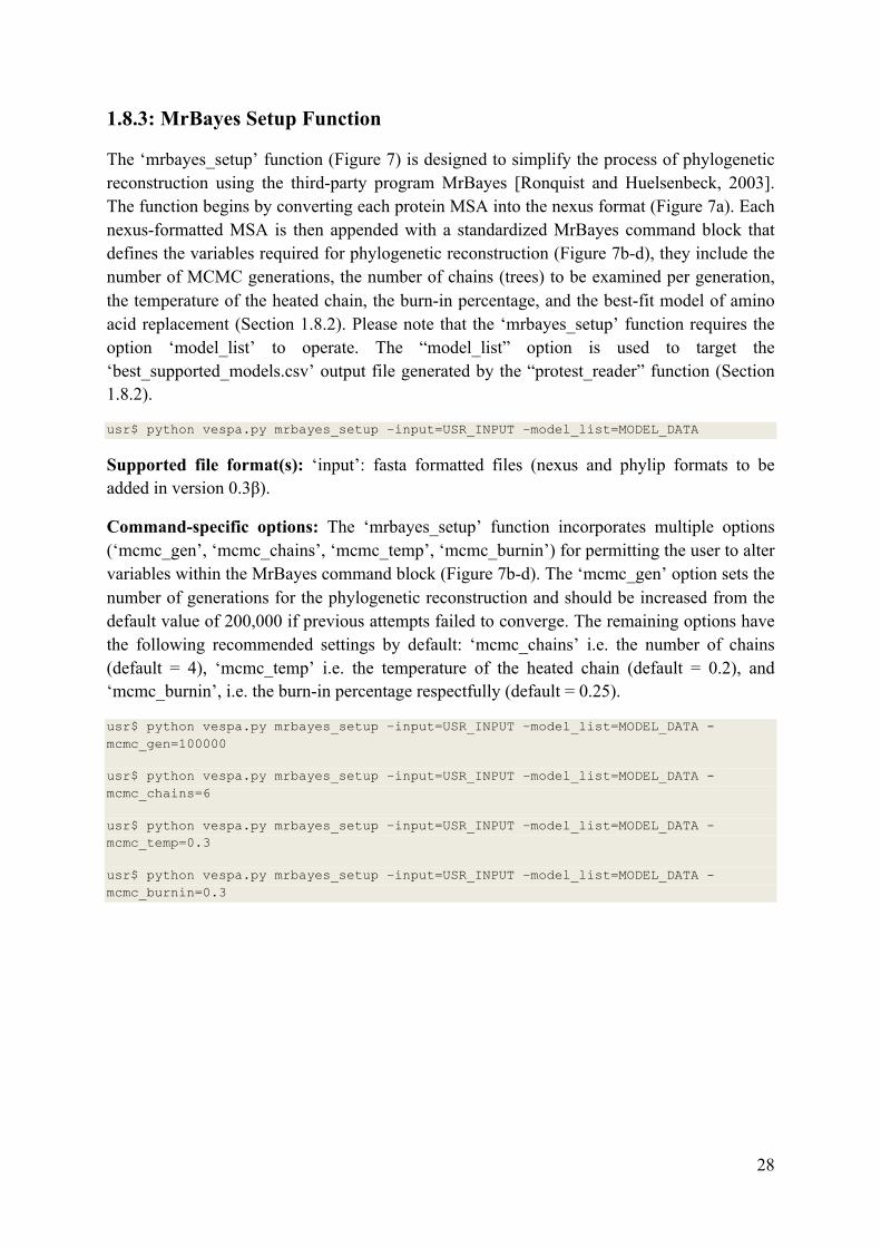
The ‘mrbayes_setup’ function (Figure 7) is designed to simplify the process of phylogenetic reconstruction using the third-party program MrBayes [Ronquist and Huelsenbeck, 2003]. The function begins by converting each protein MSA into the nexus format (Figure 7a). Each nexus-formatted MSA is then appended with a standardized MrBayes command block that defines the variables required for phylogenetic reconstruction (Figure 7b-d), they include the number of MCMC generations, the number of chains (trees) to be examined per generation, the temperature of the heated chain, the burn-in percentage, and the best-fit model of amino acid replacement (Section 1.8.2). Please note that the ‘mrbayes_setup’ function requires the option ‘model_list’ to operate. The “model_list” option is used to target the ‘best_supported_models.csv’ output file generated by the “protest_reader” function (Section 1.8.2).

usr$ python vespa.py mrbayes_setup –input=USR_INPUT –model_list=MODEL_DATA

Supported file format(s): ‘input’: fasta formatted files (nexus and phylip formats to be added in version 0.3β).

Command-specific options: The ‘mrbayes_setup’ function incorporates multiple options (‘mcmc_gen’, ‘mcmc_chains’, ‘mcmc_temp’, ‘mcmc_burnin’) for permitting the user to alter variables within the MrBayes command block (Figure 7b-d). The ‘mcmc_gen’ option sets the number of generations for the phylogenetic reconstruction and should be increased from the default value of 200,000 if previous attempts failed to converge. The remaining options have the following recommended settings by default: ‘mcmc_chains’ i.e. the number of chains (default = 4), ‘mcmc_temp’ i.e. the temperature of the heated chain (default = 0.2), and ‘mcmc_burnin’, i.e. the burn-in percentage respectfully (default = 0.25).

usr$ python vespa.py mrbayes_setup –input=USR_INPUT –model_list=MODEL_DATA -mcmc_gen=100000

usr$ python vespa.py mrbayes_setup –input=USR_INPUT –model_list=MODEL_DATA -mcmc_chains=6

usr$ python vespa.py mrbayes_setup –input=USR_INPUT –model_list=MODEL_DATA -mcmc_temp=0.3

usr$ python vespa.py mrbayes_setup –input=USR_INPUT –model_list=MODEL_DATA -mcmc_burnin=0.3

29

Figure 7: Overview of ‘mrbayes_setup function.

Figure 7 Legend The MrBayes input file is described as follows: (a) The NEXUS file is separated into two blocks, a sequence alignment block and a MrBayes command block. (b) The specific commands within the MrBayes command block are each assigned default values (in bold) based on recommend values and previous commands. (c) The commands lset and prset by default are automatically assigned by VESPA from the ‘best_supported_models.csv’ file (Section 1.8.2) specified by the “model_list” option. (d) The remaining commands are assigned based on recommended values, but may configured by the user is desired.

TLR3.nexus

#NEXUS

BEGIN DATA;DIMENSIONS NTAX=12 NCHAR=275;FORMAT DATATYPE=PROTEIN MISSING=- INTERLEAVE;

MATRIXMouse|Tlr3 MKGCSSYLMY SFGGLLSLWI LLVSSTNQCT VRYNVADCSHuman|TLR3 MRQTLPCIYF WGGLLPFGML CASSTTKCTV SHE-VADCSDog|TLR3 MSQSLLYHIY SFLGLLPFWI LCTSSTNKCV VRHEVADCS

Mouse|Tlr3 HLKLTHIPDD LPSNITVLNL T...SRNSAHHuman|TLR3 HLKLTQVPDD LPTNITVLNL T...SKNSVHDog|TLR3 HLKLTQVPDD LPANITVLNL T...SRNSIH

;END;

begin mrbayes;log start filename=TLR3_nexus.log replace;set autoclose=yes;lset applyto=(all) nst=4 rates=gamma;prset aamodelpr=fixed(jones);mcmcp ngen=200000 printfreq=2000 samplefreq=200 nchains=4 temp=0.2 savebrlens=yes relburnin=yes burninfrac=0.25;mcmc;sumt;sump;log stop;end;

Alig

nmen

t Blo

ckM

rBay

es C

omm

and

Bloc

k

lset applyto=(all) nst=4 rates=gamma;prset aamodelpr=fixed(jones);

Assigned by ProtTest

mcmcp ngen=200000 printfreq=2000 samplefreq=200 nchains=4 temp=0.2 savebrlens=yes relburnin=yes burninfrac=0.25;

ngen=200000 Assigned by command ‘mcmc_gen’nchains=4 Assigned by command ‘mcmc_chains’temp=0.2 Assigned by command ‘mcmc_temp’burninfrac=0.25 Assigned by command ‘mcmc_burnin’

a

b

c

d

lset applyto=(all) nst=4 rates=gamma;prset aamodelpr=fixed(jones);mcmcp ngen=200000 printfreq=2000 samplefreq=200 nchains=4 temp=0.2 savebrlens=yes relburnin=yes burninfrac=0.25;

30

1.9: Phase Four: Selection Analysis Preparation

The fourth phase of VESPA automates large-scale selective pressure analysis using codeML from the PAML package [Yang, 2007]. Phase four is characterized by specific commands for the basic and advanced pipeline options (Figure 1). These pipeline-associated functions are designed to process the specific input of each pipeline into a standardized file format for the common functions used by both pipelines. Following standardization, VESPA automates the normally labor-intensive process of creating the necessary files and directory structures for codeML. Phase four also incorporates a single optional function ‘branch-label table’ (Section 1.9.6) that may be invoked to enable the branch-site models of codeML [Yang, 2007].

31

1.9.1: Alignment Mapping Function

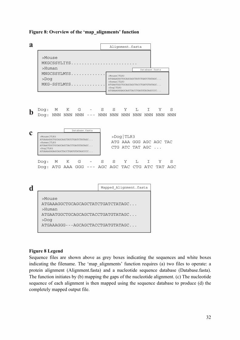
The ‘map_alignments’ function is designed to automate the conversion of protein MSAs to nucleotide MSAs (Figure 8). This process is mandatory as the codon substitution models of codeML require nucleotide alignments. Protein-MSA guided nucleotide MSAs are generated rather than directly generating nucleotide MSAs because: i) each column within the protein MSA represents aligned codons and therefore avoids aligning incomplete codons or frame-shift mutations, and ii) protein MSAs represent a comparison of the phenotype-producing elements of protein-coding sequences (Figure 8a). The function begins by reading the protein MSA to map the non-gap position of each codon within the inferred nucleotide alignment (Figure 8b). The sequence of the mapped codons is then inferred using the nucleotide dataset (preferably as a database) from earlier in the pipeline (Figure 8c). If the mapping process results in no errors, the respective nucleotide MSA is created (Figure 8d). All errors detected by the function will be returned within a separate log file. Please note that the ‘map_alignments’ function requires the option ‘database’ to indicate the nucleotide dataset for correct sequence inference.

usr$ python vespa.py map_alignments –input=USR_INPUT –database=USR_DB

Supported file format(s): ‘input’: fasta formatted files (nexus and phylip formats to be added in version 0.3β); ‘database: fasta formatted files.

32

Figure 8: Overview of the ‘map_alignments’ function

Figure 8 Legend Sequence files are shown above as grey boxes indicating the sequences and white boxes indicating the filename. The ‘map_alignments’ function requires (a) two files to operate: a protein alignment (Alignment.fasta) and a nucleotide sequence database (Database.fasta). The function initiates by (b) mapping the gaps of the nucleotide alignment. (c) The nucleotide sequence of each alignment is then mapped using the sequence database to produce (d) the completely mapped output file.

Mapped_Alignment.fasta

>MouseATGAAAGGCTGCAGCAGCTATCTGATCTATAGC...>HumanATGAATGGCTGCAGCAGCTACCTGATGTATAGC...>DogATGAAAGGG---AGCAGCTACCTGATGTATAGC...

a

d

c

Dog: M K G - S S Y L I Y SDog: NNN NNN NNN --- NNN NNN NNN NNN NNN NNN NNN

Dog: M K G - S S Y L I Y SDog: ATG AAA GGG --- AGC AGC TAC CTG ATC TAT AGC

b

Alignment.fasta

>MouseMKGCSSYLIYS.........................>HumanMNGCSSYLMYS.........................>DogMKG-SSYLMYS.........................

Database.fasta

>Mouse|TLR3ATGAAAGGCTGCAGCAGCTATCTGATCTATAGC...>Human|TLR3ATGAATGGCTGCAGCAGCTACCTGATGTATAGC...>Dog|TLR3ATGAAAGGGAGCAGCTACCTGATGTATAGCCCC...

Database.fasta

>Mouse|TLR3ATGAAAGGCTGCAGCAGCTATCTGATCTATAGC...>Human|TLR3ATGAATGGCTGCAGCAGCTACCTGATGTATAGC...>Dog|TLR3ATGAAAGGGAGCAGCTACCTGATGTATAGCCCC...

>Dog|TLR3ATG AAA GGG AGC AGC TAC CTG ATC TAT AGC ...

33

1.9.2: Gene Tree Inference Function

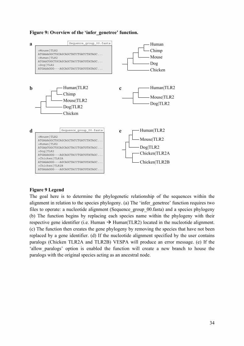
The ‘infer_genetree’ function is designed to automate the creation of the corresponding gene tree for a user-specified MSA. This is achieved by associating the taxa specified on a user-defined species tree with the headers created by ‘label_filename’ and ‘infer_ensembl_species’ (Section 1.6.1) within the MSA. The function operates by first creating a copy of the species tree with the species names (Figure 9a). The species tree is designated using the required ‘species_tree’ option.The species names are then replaced with their associated MSA headers (Figure 9b). If any species names remain after this phase, the taxa and their respective branches are removed from the tree to create the finished gene tree (Figure 9c). It should be noted that the ‘infer_genetree’ function incorporates the non-standard python library dendropy [Sukumaran et al., 2010], details on this requirement can be found in Section 1.11.

usr$ python vespa.py infer_genetree –input=USR_INPUT –species_tree=USR_INPUT

Command-specific options: The ‘infer_genetree’ function incorporates a single option ‘allow_paralogs’ that is disabled by default. Normally, ‘infer_genetree’ is designed to only allow a single MSA header to associate with a species name (Figure 9d). If multiple headers are found to associate with a species name, VESPA will produce a warning message. The ‘allow_paralogs’ may be enabled in these situations if the association error(s) are caused by within-species paralogs, in this case a gene tree will be created with associated headers shown as within-species paralogs (Figure 9e).

usr$ python vespa.py infer_genetree –input=USR_INPUT –species_tree=USR_INPUT -allow_paralogs=True

Supported file format(s): ‘input’: fasta formatted files (nexus and phylip formats to be added in version 0.3β); ‘species_tree: newick formatted files (nexus tree format to be added in version 0.3β)

34

Figure 9: Overview of the ‘infer_genetree’ function.

Figure 9 Legend The goal here is to determine the phylogenetic relationship of the sequences within the alignment in relation to the species phylogeny. (a) The ‘infer_genetree’ function requires two files to operate: a nucleotide alignment (Sequence_group_00.fasta) and a species phylogeny (b) The function begins by replacing each species name within the phylogeny with their respective gene identifier (i.e. Human à Human|TLR2) located in the nucleotide alignment. (c) The function then creates the gene phylogeny by removing the species that have not been replaced by a gene identifier. (d) If the nucleotide alignment specified by the user contains paralogs (Chicken TLR2A and TLR2B) VESPA will produce an error message. (e) If the ‘allow_paralogs’ option is enabled the function will create a new branch to house the paralogs with the original species acting as an ancestral node.

a Sequence_group_00.fasta

>Mouse|TLR2ATGAAAGGCTGCAGCAGCTATCTGATCTATAGC...>Human|TLR2ATGAATGGCTGCAGCAGCTACCTGATGTATAGC...>Dog|TLR2ATGAAAGGG---AGCAGCTACCTGATGTATAGC...

HumanChimpMouseDogChicken

b Human|TLR2ChimpMouse|TLR2Dog|TLR2Chicken

c Human|TLR2

Mouse|TLR2Dog|TLR2

Sequence_group_00.fasta

>Mouse|TLR2ATGAAAGGCTGCAGCAGCTATCTGATCTATAGC...>Human|TLR2ATGAATGGCTGCAGCAGCTACCTGATGTATAGC...>Dog|TLR2ATGAAAGGG---AGCAGCTACCTGATGTATAGC...>Chicken|TLR2AATGAAAGGG---AGCAGCTACCTGATGTATAGC...>Chicken|TLR2BATGAAAGGG---AGCAGCTACCTGATGTATAGC...

d Human|TLR2

Mouse|TLR2

Dog|TLR2Chicken|TLR2A

Chicken|TLR2B

e

35

1.9.3: CodeML Setup Function

The ‘codeml_setup’ function is designed to simplify the creation of the complex codeML directory structure. This is achieved by incorporating previously written in-house software ‘GenerateCodemlWorkspace.pl’ written by Dr. Thomas Walsh to produce the codeML directory structure [Walsh, 2013]. The purpose of automating the program ‘GenerateCodemlWorkspace.pl’ via ‘setup_codeml’ was to simplify input requirements and enable high-throughput analyses. The function requires only a protein-inferred nucleotide MSA (Section 1.9.1) and an associated phylogenetic tree (Section 1.9.2 or 1.9.4) to construct the directory structure for the codeML site-specific models [Walsh, 2013].

usr$ python vespa.py codeml_setup –input=USR_INPUT

Supported file format(s): ‘input’: newick formatted files (nexus tree format to be added in version 0.3β)

Command-specific options: If the user has created the optional branch-label table (Section 1.9.6) and enabled the ‘label_table’ option the function will create the directory structure for the codeML branch-site models. Automating the branch-site models requires a specific directory for each species and/or lineage specified by the user in the optional branch-label table (Figure 10a). Next the ‘setup_codeml’ function will produce a codeML “taskfile” that contains each codeML command line command to be computed (Figure 10b). Following creation of the taskfile, a separate log file reporting the branch-site models that cannot be tested (due to missing taxa) is produced.

usr$ python vespa.py codeml_setup –input=USR_INPUT –label_table=USR_INPUT

36

Figure 10: Overview of the ‘codeml_setup’ function.

Figure 10 Legend (a) Using the branch-label table (branch_table.txt) the function produces species-labelled (highlighted) phylogenies for each species or ancestral node specified and then automates the production of the codeML directory for the branch-site models. (b) The function terminates by producing a codeML taskfile with all the codeML command line commands required to complete the job.

a branch_table.txt

MouseHumanEglires: Human, Mouse

codeml_taskfile.txt

cd CodeML/TLR2/TLR2_Human/modelA/Omega0/; codemlcd CodeML/TLR2/TLR2_Human/modelA/Omega10/; codemlcd CodeML/TLR2/TLR2_Human/modelA/Omega1/; codemlcd CodeML/TLR2/TLR2_Human/modelA/Omega2/; codemlcd CodeML/TLR2/TLR2_Mouse/modelA/Omega1/; codemlcd CodeML/TLR2/TLR2_Mouse/modelA/Omega2/; codemlcd CodeML/TLR2/TLR2_Mouse/modelA/Omega0/; codemlcd CodeML/TLR2/TLR2_Mouse/modelA/Omega10/; codemlcd CodeML/TLR2/TLR2_Eglires/modelA/Omega10/; codemlcd CodeML/TLR2/TLR2_Eglires/modelA/Omega2/; codemlcd CodeML/TLR2/TLR2_Eglires/modelA/Omega1/; codemlcd CodeML/TLR2/TLR2_Eglires/modelA/Omega0/; codeml

b

Human|TLR2

Mouse|TLR2


Chicken|TLR2B

MouseSequence_group_00.fasta












Human|TLR2

Mouse|TLR2


Chicken|TLR2B

Mouse













CodeML Directory

Human|TLR2

Mouse|TLR2


Chicken|TLR2B

Human













CodeML DirectorySequence_group_00.fasta












CodeML DirectoryEglieres

Human|TLR2

Mouse|TLR2


Chicken|TLR2B

37

1.9.4: MrBayes Reader Function

If phylogenetic reconstruction has been performed by MrBayes then the ‘mrbayes_reader’ function is designed to replace ‘infer_genetree’ [Ronquist and Huelsenbeck, 2003]. The function operates by converting the nexus-formatted phylogeny into the newick format supported by VESPA and codeML [Yang 2007]. If the function is unable to locate the original amino acid fasta-formatted MSA required by ‘mrbayes_setup’ (Section 1.8.3) the nexus-formatted MSA will be converted and placed with the newick-formatted phylogeny. It should be noted that ‘mrbayes_reader’ is unable to check phylogenies for convergence. Instead users are directed to confirm convergence using third party software such as Tracer [Rambaut et al., 2014].

usr$ python vespa.py mrbayes_reader –input=USR_INPUT

Supported file format(s): ‘input’: MrBayes standard output format.

38

1.9.5: Subtree Function

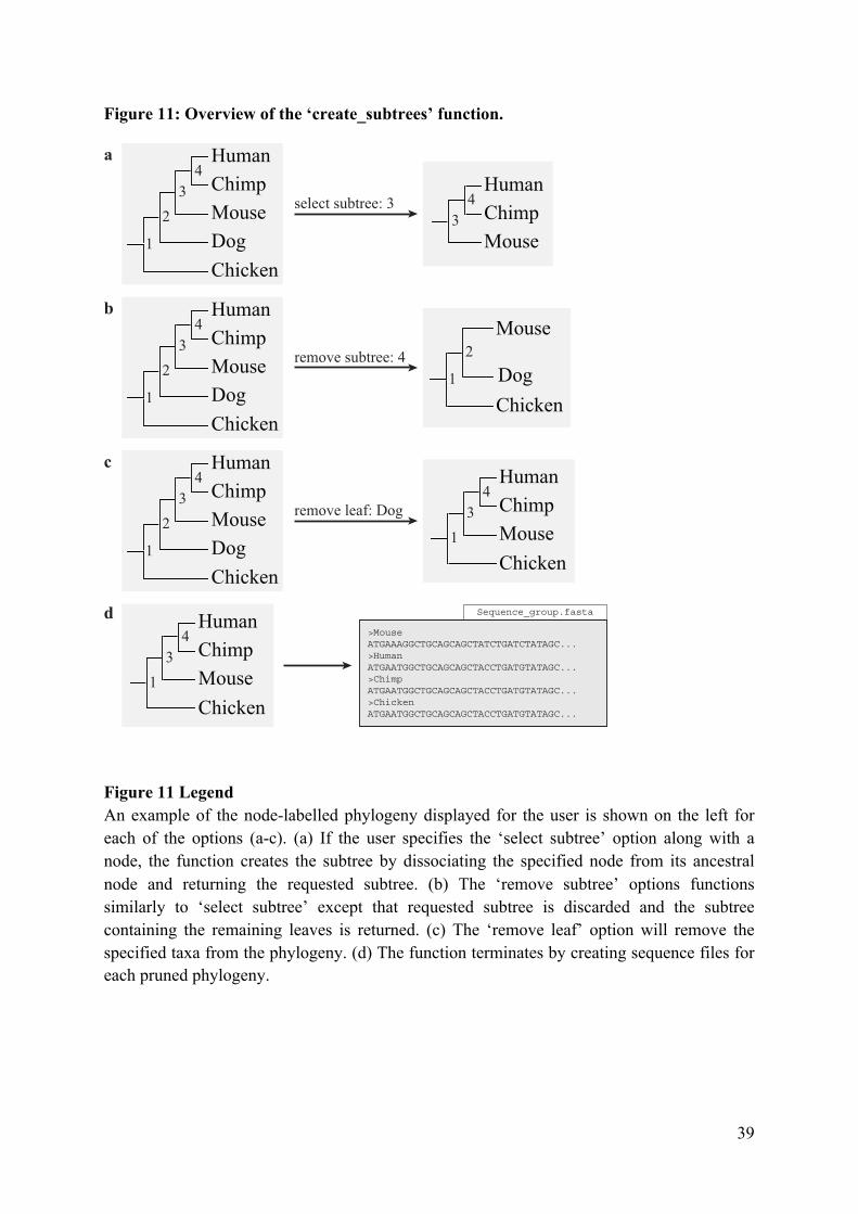
The ‘create_subtrees’ function is designed for high-throughput tree pruning. This optional step is often required to prune very large multigene family phylogenies into smaller sub-phylogenies. Larger phylogenies may require this pruning step due to feasibility concerns and as subfamilies decrease computational requirements whilst making data easier to manage we have included this optional function. Users may require this option for pruning out SGOs for selection analyses that are focused on single genes. The function operates by displaying the current phylogeny with a set of pruning commands/options. The user is then prompted to select one of the four commands: ‘select subtree’, ‘remove subtree’, ‘remove leaf’, or ‘keep original’. If either ‘select subtree’ or ‘remove subtree’ is selected, the user is prompted to select a single node (numbered on the displayed phylogeny) for selection or removal respectively (Figure 11a/b). If ‘remove leaf’ is selected, the user is prompted to select a leaf label (sequence header) for removal (Figure 11c). If ‘keep original’ is selected the tree manipulation step is skipped. The ‘create_subtrees’ function will produce a protein sequence file of the remaining nodes in the phylogeny (Figure 11d). The protein sequence file is then required to undergo re-alignment and it proceeds from Phase 3 through the remainder of the pipeline (Figure 1). The ‘create_subtrees’ function will also produce a separate log file of the original phylogeny, the selected command, and the resulting phylogeny. The ‘create_subtrees’ function incorporates the non-standard python library dendropy [Sukumaran et al., 2010] (Section 1.10).

usr$ python vespa.py create_subtree –input=USR_INPUT


39

Figure 11: Overview of the ‘create_subtrees’ function.

Figure 11 Legend An example of the node-labelled phylogeny displayed for the user is shown on the left for each of the options (a-c). (a) If the user specifies the ‘select subtree’ option along with a node, the function creates the subtree by dissociating the specified node from its ancestral node and returning the requested subtree. (b) The ‘remove subtree’ options functions similarly to ‘select subtree’ except that requested subtree is discarded and the subtree containing the remaining leaves is returned. (c) The ‘remove leaf’ option will remove the specified taxa from the phylogeny. (d) The function terminates by creating sequence files for each pruned phylogeny.


1

23

4

select subtree: 3


1

23

4

remove subtree: 4


1

23

4

remove leaf: Dog

a

b

c

HumanChimpMouse

34

Mouse

DogChicken

1

2

HumanChimpMouseChicken

13

4

Sequence_group.fasta

>MouseATGAAAGGCTGCAGCAGCTATCTGATCTATAGC...>HumanATGAATGGCTGCAGCAGCTACCTGATGTATAGC...>ChimpATGAATGGCTGCAGCAGCTACCTGATGTATAGC...>ChickenATGAATGGCTGCAGCAGCTACCTGATGTATAGC...

HumanChimpMouseChicken

13

4d

40

1.9.6: Create Branch Table Function

The ‘create_branch’ function is designed to simplify the creation of the branch-label table required for the branch-site models of codeML [Yang 2007]. The branch-label table (previously shown in Figure 10a) indicates the lineages or ‘branches’ that will undergo lineage-specific selection analysis, i.e. designation of the “foreground lineages” for codeML. Each line indicates one lineage, either a species or an ancestral node. Ancestral nodes (uniquely named by user [i.e. Eglires]) are followed by a list of descendant (extant) species (Figure 10a). The function operates by displaying a user-specified species phylogeny and promoting the user to select the species and/or ancestral nodes (numbered on the displayed phylogeny) of interest for the study (identical display methodology as described in Section 1.9.4 - see phylogeny in Figure 11a for example). When the user has finished their selection, the function will automatically produce the branch-label table. It should be noted that this function is completely optional as the branch-label table may be easily created by hand. The ‘create_branch’ function incorporates the non-standard python library dendropy [Sukumaran et al., 2010] (Section 1.10).

usr$ python vespa.py create_branch –input=USR_INPUT


41

1.10: Phase Five: Selection Analysis Assessment

1.10.1: CodeML Results Assessment Function

The ‘codeml_reader’ function is designed to parse the complex codeML directory structure and create simplified results for inexperienced users. This is achieved by incorporating in-house software ‘CreateSummaryReport.pl’ written by Dr. Thomas Walsh [Walsh, 2013] to produce the majority of the codeML results. In addition to automating ‘CreateSummaryReport.pl’, ‘codeml_reader’ produces supplementary output files (Figure 12) and specialized MSAs that are designed to aid in the detection of false positives (Figure 13). If the user specifies a branch-label table (Section 2.9.6) ‘codeml_reader’ will produce codeML MSAs, these MSAs are characterized by the addition of i) the putative positively selected sites, and ii) the codons/amino acids that are positively selected in the respective lineage/s.

usr$ python vespa.py codeml_reader –input=USR_INPUT

Supported file format(s): ‘input’: VESPA formatted codeML standard output.

42

Figure 12: Sample supplementary output file created by ‘codeml_reader’

Figure 12 Legend The supplementary output file includes information for each site-specific and branch-specific model of codeML. The following information is provided for each model: the tree tested; the type of model (i.e. site-specific or branch-specific) being tested; number of free parameters in the ω

Model Tree Model(Type pw((t=0) lnL LRT(Result Parameter(Estimates

Positive(Selection

Positively(Selected(Sites(in(8x45(Alignment((P(w>1)(>(0.5)

m0 Sample_MSA Homogeneous 1 2 J572.969394 N/A w=0.61924 No

m1Neutral Sample_MSA SiteJspecific 1 2 J568.572319 N/A p0=0.35065(p1=0.64935(w0=0.08403(w1=1.00000 Not(Allowed

m2Selection Sample_MSA SiteJspecific 2 2 J568.521978 m1Neutral p0=0.37699(p1=0.00000(p2=0.62301(w0=0.10174(w1=1.00000(w2=1.11245

No

m3Discrtk2 Sample_MSA SiteJspecific 3 2 J568.521978 m3Discrtk2 p0=0.37699(p1=0.62301(w0=0.10174(w1=1.11245 YesAlignment((28(NEB(sites):(2(3(4(5(6(8(12(13(15(17(19(20(22(23(24(25(26(27(30(31(32(34(35(39(40(41(43(44

m3Discrtk3 Sample_MSA SiteJspecific 5 2 J568.521978 m3Discrtk2 p0=0.37699(p1=0.53897(p2=0.08404(w0=0.10174(w1=1.11245(w2=1.11246

No

m7 Sample_MSA SiteJspecific 2 2 J568.764172 N/A p=0.22135(q=0.11441 Not(Allowed

m8 Sample_MSA SiteJspecific 4 2 J568.526486 m7,(m8a p=11.60971(p0=0.37916(p1=0.62084(q=99.00000(w=1.11431

No

m8a Sample_MSA SiteJspecific 4 1 J568.578069 N/A p=9.38528(p0=0.35203(p1=0.64797(q=99.00000(w=1.00000

Not(Allowed

modelA Sample_MSA_Primates BranchJsite 3 2 J568.572319 m1Neutral,(modelAnull

p0=0.35065(p1=0.64935(p2=0.00000(p3=0.00000(w0=0.08403(w1=1.00000(w2=1.00000

No

modelAnull Sample_MSA_Primates BranchJsite 3 1 J568.572319 N/A p0=0.35065(p1=0.64935(p2=0.00000(p3=0.00000(w0=0.08403(w1=1.00000(w2=1.00000

Not(Allowed

modelA Sample_MSA_Chimp BranchJsite 3 2 J557.052657 modelA p0=0.33452(p1=0.59186(p2=0.02659(p3=0.04704(w0=0.10990(w1=1.00000(w2=999.00000

Yes Alignment((3(BEB(sites):(24(25(32

modelAnull Sample_MSA_Chimp BranchJsite 3 1 J568.572319 N/A p0=0.35065(p1=0.64935(p2=0.00000(p3=0.00000(w0=0.08403(w1=1.00000(w2=1.00000

Not(Allowed

modelA Sample_MSA_Human BranchJsite 3 2 J568.572319 m1Neutral,(modelAnull

p0=0.35065(p1=0.64935(p2=0.00000(p3=0.00000(w0=0.08403(w1=1.00000(w2=1.00000

No

modelAnull Sample_MSA_Human BranchJsite 3 1 J568.572319 N/Ap0=0.35065(p1=0.64935(p2=0.00000(p3=0.00000(w0=0.08403(w1=1.00000(w2=1.00000

Not(Allowed

43

distribution that are estimated by codeML, the initial ω value used by codeML; the resulting log likelihood (lnL) of the analysis; the resulting model of the likelihood ratio test (LRT); the parameter estimates of codeML; if positive selection was detected; and the positively selected sites (if positive selection was detected).

44

Figure 13: Sample specialized MSA created by ‘codeml_reader’

Figure 13 Legend The specialized MSA shown above includes data on the location of positively selected codons or residues. Depending on the type of model being explored, the MSA will include additional information. For all models (site-specific or branch-specific), the header ‘PS_Sites’ indicates the position of the positively selected codons (shown as NNN) or residues (shown as X). For branch-specific, the characters under positive selection are shown for each relevant lineage using the header ‘PS_Characters’ followed the by the lineage of interest (i.e. PS_Characters|Chimp above).

45

1.11: Software dependencies The VESPA software package is designed to minimize potential software dependencies, as additional software requirements may be difficult for users to install on their systems. Currently, the non-standard python library dendropy [Sukumaran et al., 2010] is the only dependency that remains in VESPA. Dendropy incorporates numerous functions for storing phylogenetic information and simplifying tree-based analyses. Dendropy can be installed from here (https://pythonhosted.org/DendroPy/). Removal of dendropy would require substantial development time and the design of numerous core functions. However, installation of dendropy is simple and only requires a single command to be invoked by the user. If the user invokes a dendropy-dependent function, VESPA is designed to print a warning message detailing the installation process of dendropy if the software is not installed.

46

1.12: Third-Party Programs

The VESPA software package is designed to interface with a number of third-party programs. It should be noted that some functions were designed to interface with specific versions of these third-party programs and future updates may require updates to VESPA as well. Details on these third-party programs can be found below.

Program Version Program Link BLAST 2.2.30+ ftp://ftp.ncbi.nlm.nih.gov/blast/executables/blast+/LATEST/ DendroPy 4.0 https://pythonhosted.org/DendroPy/#installing MetAL 1.1 http://kumiho.smith.man.ac.uk/blog/whelanlab/?page_id=396

MrBayes 3.2.3 http://mrbayes.sourceforge.net/

MUSCLE 3.8.21 http://www.drive5.com/muscle/downloads.htm

NoRMD 1.3 ftp://ftp-igbmc.u-strasbg.fr/pub/NORMD/

PAML 4.4e http://abacus.gene.ucl.ac.uk/software/paml.html

ProtTest3 3.4 https://code.google.com/p/prottest3/

47

1.13: References

Altschul SF, Gish W, Miller W, Myers EW, Lipman DJ. 1990. Basic local alignment search tool. Journal of Molecular Biology 215:403-410.

Blackburne BP, Whelan S. 2012. Measuring the distance between multiple sequence alignments. Bioinformatics 28:495-502.

Darriba D, Taboada GL, Doallo R, Posada D. 2011. ProtTest 3: fast selection of best-fit models of protein evolution. Bioinformatics 27:1164-1165.

Eddy SR. 1998. Profile hidden Markov models. Bioinformatics 14:755-763.

Fletcher W, Yang ZH. 2010. The Effect of Insertions, Deletions, and Alignment Errors on the Branch-Site Test of Positive Selection. Molecular Biology and Evolution 27:2257-2267.

Keane TM, Creevey CJ, Pentony MM, Naughton TJ, McInerney JO. 2006. Assessment of methods for amino acid matrix selection and their use on empirical data shows that ad hoc assumptions for choice of matrix are not justified. BMC Evolutionary Biology 6.

Rambaut A, Suchard M, Xie D, Drummond A. 2014. Tracer v1.6, Available from http://beast.bio.ed.ac.uk/Tracer.

Ronquist F. 2011. Draft MrBayes version 3.2 Manual: Tutorials and Model Summaries [Internet]. Available from: http://mrbayes.sourceforge.net/mb3.2_manual.pdf

Sukumaran J, Holder MT. 2010. DendroPy: a Python library for phylogenetic computing. Bioinformatics 26:1569-1571.

Thompson JD, Plewniak F, Ripp R, Thierry JC, Poch O. 2001. Towards a reliable objective function for multiple sequence alignments. Journal of Molecular Biology 314:937-951.

Walsh TA. 2013. The evolution of the mammal placenta - a computational approach to the identification and analysis of placenta-specific genes and microRNAs. PhD Thesis. Dublin: Dublin City University.

Yang Z. 2007. PAML 4: phylogenetic analysis by maximum likelihood. Molecular Biology and Evolution 24:1586-1591.

Webb VESPA Manual - dfzljdn9uc3pi.cloudfront.net fileThe VESPA (Very large-scale Evolution and...

Documents

Transcript of Webb VESPA Manual - dfzljdn9uc3pi.cloudfront.net fileThe VESPA (Very large-scale Evolution and...