Wavelet basicsHennie ter Morsche

1. Introduction

2. The continuous/discrete wavelet transform

3. Multi-resolution analysis

4. Scaling functions

5. The Fast Wavelet Transform

6. Examples

1

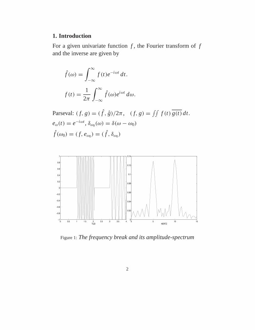
1. Introduction

For a given univariate function f , the Fourier transform of fand the inverse are given by

f (ω) =∫ ∞

−∞f (t)e−iωt dt .

f (t) = 1

2π

∫ ∞

−∞f (ω)eiωt dω.

Parseval: ( f, g) = ( f , g)/2π , ( f, g) = ∫∫f (t) g(t)dt .

eω(t) = e−iωt , δω0(ω) = δ(ω − ω0)

f (ω0) = ( f, eω0) = ( f , δω0)

0 0.5 1 1.5 2 2.5 3 3.5 4−1

−0.8

−0.6

−0.4

−0.2

0

0.2

0.4

0.6

0.8

1

TIJD0 5 10 15

0

0.02

0.04

0.06

0.08

0.1

0.12

0.14

HERTZ

Figure 1: The frequency break and its amplitude-spectrum

2

The short time Fourier transform

Given a Window function g

g ∈ L2(IR), ‖g‖ = 1 g is real-valued.

The short time Fourier transform F(u, τ ) of a function f isdefined by

F(u, τ ) =∫ ∞

−∞f (t)e−iut g(t − τ) dt,

f (t) = 1

2π

∫ ∞

−∞

∫ ∞

−∞F(u, τ )eiutg(t − τ) dτ du,

gu,τ (t) := eiut g(t − τ), F(u, τ ) = ( f, gu,τ )

( f, gu,τ ) = 1

2π( f , gu,τ ) ( Parseval).

gu,τ (ω) = e−i(ω−u)τ g(ω − u).

Fixed ” window width” in time and frequency.

3

2. The continous/discrete Wavelet transform

The continuous Wavelet transform

Given ψ in L2(IR).Introduce a family of functionsψa,b (a > 0, b ∈ IR) as follows

ψa,b(t) = 1√aψ((t − b)/a) (t ∈ IR),

‖ψa,b‖ = ‖ψ‖.

The continuous wavelet transform F(a, b) of a function f isdefined by

F(a, b) = ( f, ψa,b) = 1√a

∫ ∞

−∞f (t) ψ((t − b)/a) dt .

( f, ψa,b) = 1

2π( f , ψa,b) Parseval.

where

ψa,b(ω) = √a e−iωbψ(aω),

4

The inverse wavelet transform

f (t) = C−1ψ

∫ ∞

−∞

∫ ∞

0

1

a2F(a, b) ψa,b(t) da db.

Cψ =∫ ∞

0

|ψ(ω)|2ω

dω.

Needed ψ(0) = 0, i.e.,

∫ ∞

−∞ψ(t) dt = 0.

This is the reason why the functions ψa,b are called wavelets.

ψ is called the Motherwavelet.

5

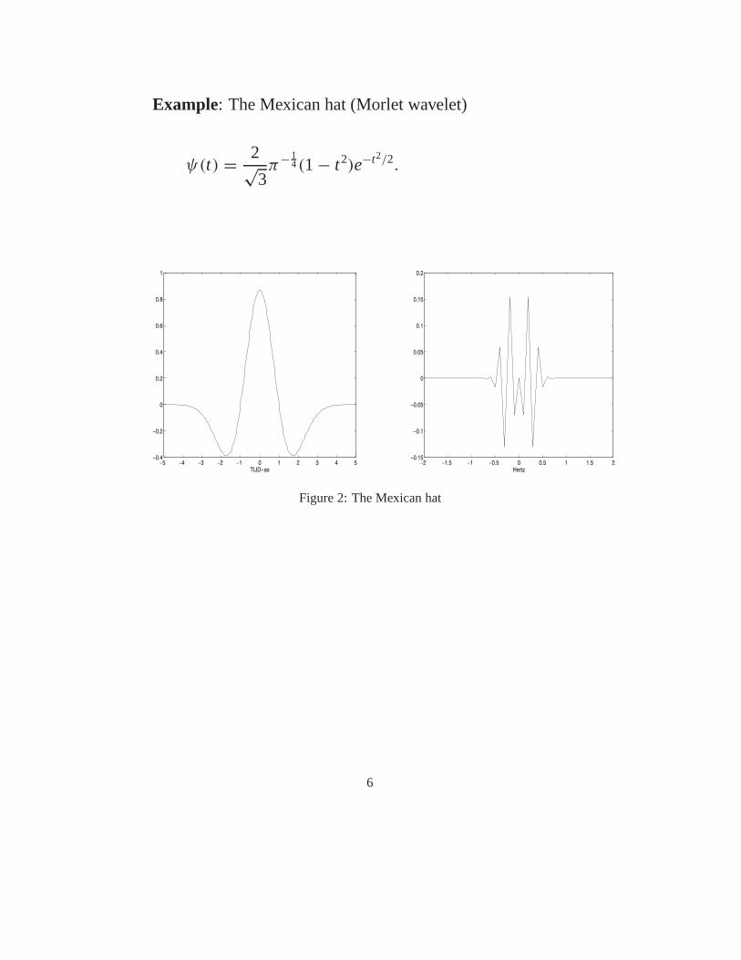
Example: The Mexican hat (Morlet wavelet)

ψ(t) = 2√3π− 1

4 (1 − t2)e−t2/2.

−5 −4 −3 −2 −1 0 1 2 3 4 5−0.4

−0.2

0

0.2

0.4

0.6

0.8

1

TIJD−as−2 −1.5 −1 −0.5 0 0.5 1 1.5 2

−0.15

−0.1

−0.05

0

0.05

0.1

0.15

0.2

Hertz

Figure 2: The Mexican hat

6

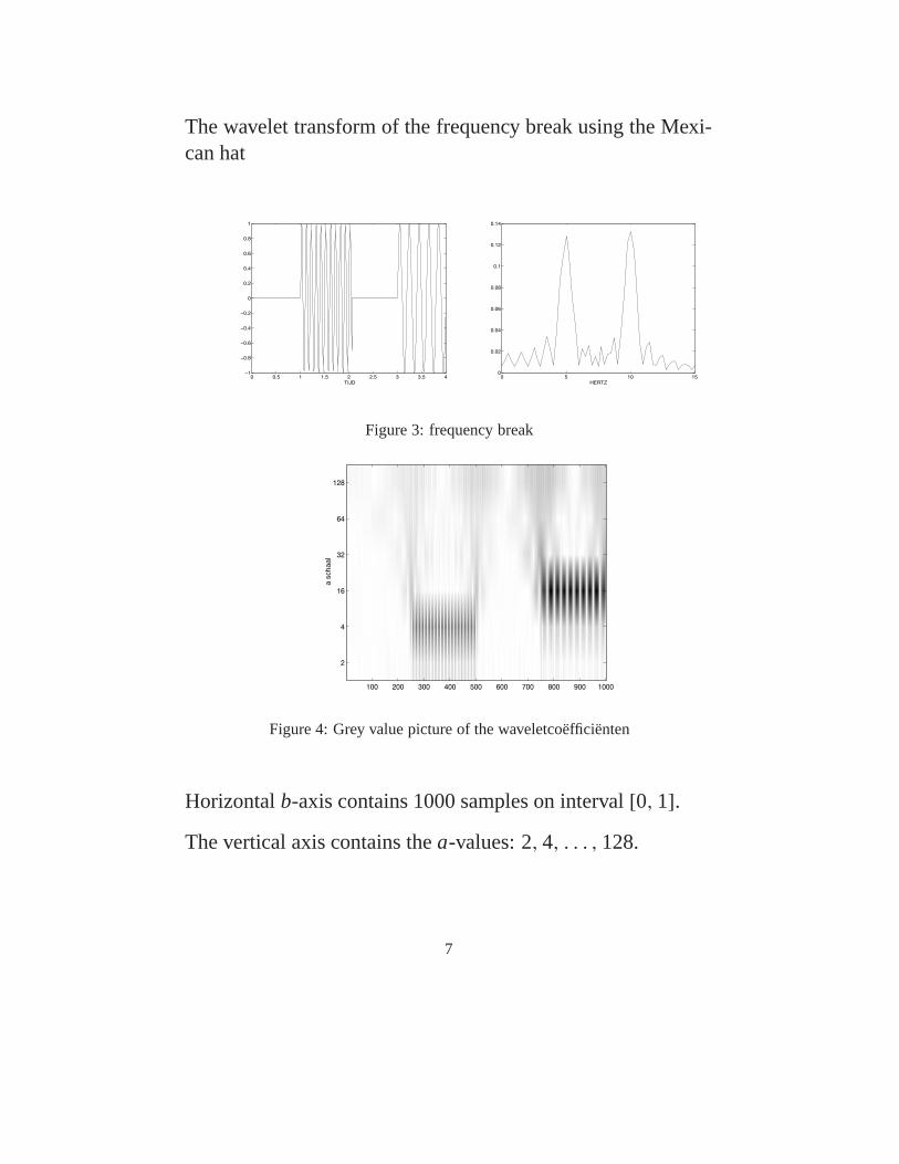
The wavelet transform of the frequency break using the Mexi-can hat

0 0.5 1 1.5 2 2.5 3 3.5 4−1

−0.8

−0.6

−0.4

−0.2

0

0.2

0.4

0.6

0.8

1

TIJD0 5 10 15

0

0.02

0.04

0.06

0.08

0.1

0.12

0.14

HERTZ

Figure 3: frequency break

a s

chaal

100 200 300 400 500 600 700 800 900 1000

2

4

16

32

64

128

Figure 4: Grey value picture of the waveletcoëfficiënten

Horizontal b-axis contains 1000 samples on interval [0, 1].The vertical axis contains the a-values: 2, 4, . . . , 128.

7

The discrete wavelet transform

Sampling in the a-b plane.

a0 > 1, b0 > 0a = a−�

0 , b = k a−�0 b0, (k, � ∈ ZZ ).

The translation step is adapted to the scale

ψk,�(t) = a�/20 ψ(a�0t − k b0).

Dyadic wavelets: a0 = 2, b0 = 1.

ψk,�(t) = 2�/2ψ(2�t − k).

( f, ψk,�) are called waveletcoefficients.

Discrete Wavelet transform: f → ( f, ψk,�)

a. Problem of reconstruction:

f = ∑k,�( f, ψk,�)ψk,�.

b. Problem of decomposition:

f = ∑k,� ak,�ψk,�

It would be nice if the functions ψk,� constitute an orthonormalbasis of L2(IR). (orthogonal wavelets)

8

For orthogonal wavelets the reconstruction formula and the de-composition formula coincide.A biorthogonal wavelets system consists of two sets of waveletsgenerated by a mother wavelet ψ and a dual wavelet ψ , forwhich

(ψk,�, ψm,n) = δk,mδ�,n,

for all integer values k, �,m en n.We assume that (ψk,�) constitute a so called Riesz basis (nu-merically stable) of L2(IR), i.e.

A ( f, f ) ≤ ‖∑k,�

ξk,�‖2 ≤ B ( f, f )

for positive constants A en B, where f = ∑k,� ξk,�ψk,�.

The reconstruction formula now reads

f =∑k,�

( f, ψk,�)ψk,�.

Examples of biorthogonal wavelets are the bior family imple-mented in the MATLAB Toolbox

9

3. Multi-resolution analysis

For a given function f , let

f� =∞∑

k=−∞( f, ψk,�)ψk,�,

Then

f =∞∑

�=−∞f�.

f� can be interpreted as that part of f which belongs to thescale �.So, f = ∑∞

�=−∞ f� is a decomposition of f to different scalelevels �.The function f� belongs to the scale space W� spanned by(ψk,�) with fixed �.

The space W0 is spanned by the integer translates of the motherwavelet ψ .

For integer n the function

gn(t) =n−1∑�=−∞

f�(t)

contains all the information of f up to scale level n − 1.So gn ∈ Vn , where

Vn =n−1∑�=−∞

W�.

It follows that Vn = Vn−1 ⊕ Wn−1 (n ∈ ZZ) direct sum.

10

Properties of the sequence (Vn)

a) Vn−1 ⊂ Vn (n geheel),

b)⋃

n∈ZZVn = L2(IR),

c)⋂

n∈ZZVn = {0},

d) f (t) ∈ Vn ⇔ f (2t) ∈ Vn+1,

e) f (t) ∈ V0 ⇒ f (t + 1) ∈ V0.

If a sequence of subspaces (Vn) satisfies the properties a) to e),then it is called a Multi-Resolution-Analysis (MRA) of L2(IR).

If there exists a function φ such that V0 is spanned by the in-teger translates of φ, then φ is called a scaling function for theMRA.As a consequence one has that Vn is spanned by φk,n, (n fixed),

φk,n = 2n/2 φ(2n t − k)

11

4. Scaling functions

Sufficient conditions for a compactly supported function φ tobe a scaling function for an MRA.

1. There exists a sequence of numbers (pk), from which only afinite number differs from zero, such that

φ(t) =∞∑

k=−∞pkφ(2t − k) 2-scale relation.

2. The so-called Riesz function has no zeros on the unit circle.

Autocorrelation function of φ: ρ(τ) := ∫ ∞−∞ φ(t + τ) φ(t) dt .

Riesz function

R(z) =∞∑

m=−∞ρ(m) zm.

3. Partition of the unity

∑k

φ(t − k) ≡ 1.

The Laurent polynomial P(z) = 12

∑k pk zk is called the two

scale symbol of φ.

12

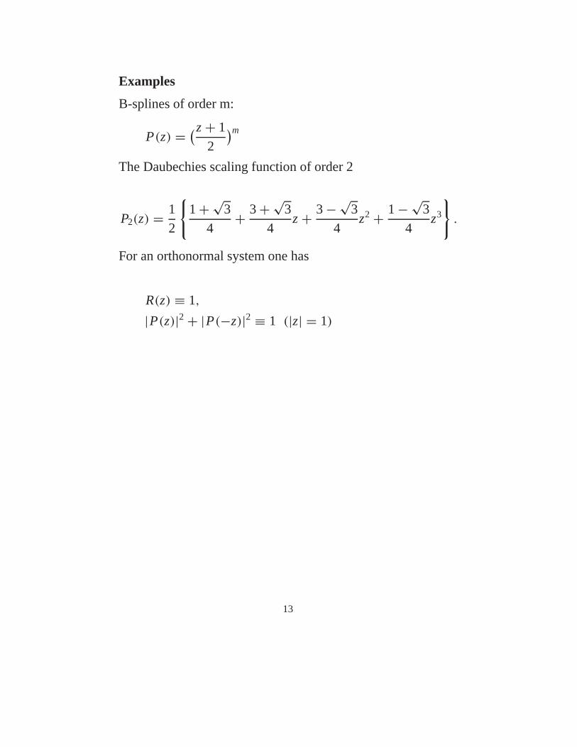
Examples

B-splines of order m:

P(z) = (z + 1

2

)m

The Daubechies scaling function of order 2

P2(z) = 1

2

{1 + √

3

4+ 3 + √

3

4z + 3 − √

3

4z2 + 1 − √

3

4z3

}.

For an orthonormal system one has

R(z) ≡ 1,

|P(z)|2 + |P(−z)|2 ≡ 1 (|z| = 1)

13

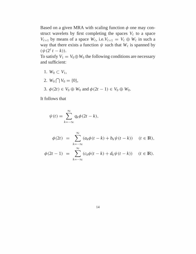
Based on a given MRA with scaling function φ one may con-struct wavelets by first completing the spaces V� to a spaceV�+1 by means of a space W�, i.e.V�+1 = V� ⊕ W� in such away that there exists a function ψ such that W� is spanned by(ψ(2� t − k)).To satisfy V1 = V0⊕W0 the following conditions are necessaryand sufficient:

1. W0 ⊂ V1,

2. W0⋂

V0 = {0},3. φ(2t) ∈ V0 ⊕ W0 and φ(2t − 1) ∈ V0 ⊕ W0.

It follows that

ψ(t) =∞∑

k=−∞qkφ(2t − k),

φ(2t) =∞∑

k=−∞(akφ(t − k)+ bkψ(t − k)) (t ∈ IR),

φ(2t − 1) =∞∑

k=−∞(ckφ(t − k)+ dkψ(t − k)) (t ∈ IR).

14

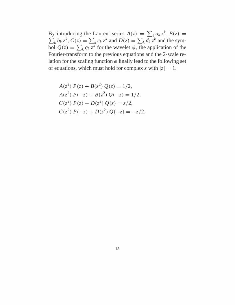
By introducing the Laurent series A(z) = ∑k ak zk, B(z) =∑

k bk zk,C(z) = ∑k ck zk and D(z) = ∑

k dk zk and the sym-bol Q(z) = ∑

k qk zk for the wavelet ψ , the application of theFourier-transform to the previous equations and the 2-scale re-lation for the scaling function φ finally lead to the following setof equations, which must hold for complex z with |z| = 1.

A(z2) P(z)+ B(z2) Q(z) = 1/2,

A(z2) P(−z)+ B(z2) Q(−z) = 1/2,

C(z2) P(z)+ D(z2) Q(z) = z/2,

C(z2) P(−z)+ D(z2) Q(−z) = −z/2,

15

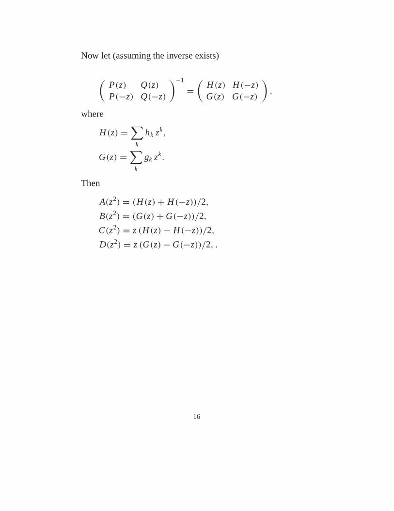
Now let (assuming the inverse exists)

(P(z) Q(z)P(−z) Q(−z)

)−1

=(

H (z) H (−z)G(z) G(−z)

),

where

H (z) =∑

k

hk zk,

G(z) =∑

k

gk zk .

Then

A(z2) = (H (z)+ H (−z))/2,

B(z2) = (G(z)+ G(−z))/2,

C(z2) = z (H (z)− H (−z))/2,

D(z2) = z (G(z)− G(−z))/2, .

16

We now have

φ(2t−k) =∞∑

m=−∞

(h2m−kφ(t−m)+g2m−kψ(t−m)

)(t ∈ IR).

It can be shown that the symbol P(z) for the dual scaling φ andthe symbol Q(z) for the dual wavelet ψ will satisfy

P(z) = H (z−1),

Q(z) = Q(z−1).

For orthogonal wavelets based on an orthogonal scaling func-tion one may choose

qk = (−1)k p1−k.

17

5. The Fast Wavelet Transform

To obtain a wavelet decomposition of a function f in practice,one first approximates f by a function from a space Vn, whichis close to f . So let us assume that f itself belongs to Vn. So

f =∞∑

k=−∞ak,nφk,n

Since Vn = ∑n−1�=−∞ W�, one has

f =n−1∑�=−∞

∞∑k=−∞

dk,�ψk,�

18

Vn = Vn−1 ⊕ Wn−1 implies

f =∞∑

k=−∞ak,nφk,n =

∞∑k=−∞

ak,n−1φk,n−1+∞∑

k=−∞dk,n−1ψk,n−1.

Due to

φk,n =∞∑

m=−∞

√2 h2m−kφm,n−1 + √

2 g2m−kψm,n−1.

we obtain

f =∞∑

k=−∞ak,nφk,n =

∞∑k=−∞

ak,n

√2 (

∞∑m=−∞

(h2m−kφm,n−1+g2m−kψm,n−1)).

Our conclusion is

am,n−1 =∞∑

k=−∞

√2 h2m−kak,n, dm,n−1 =

∞∑k=−∞

√2 g2m−kak,n.

convolution and subsequently downsampling (m → 2 m) yieldsthe two sequences a(n−1) = (am,n−1) en d (n−1) = (dm,n−1).

19

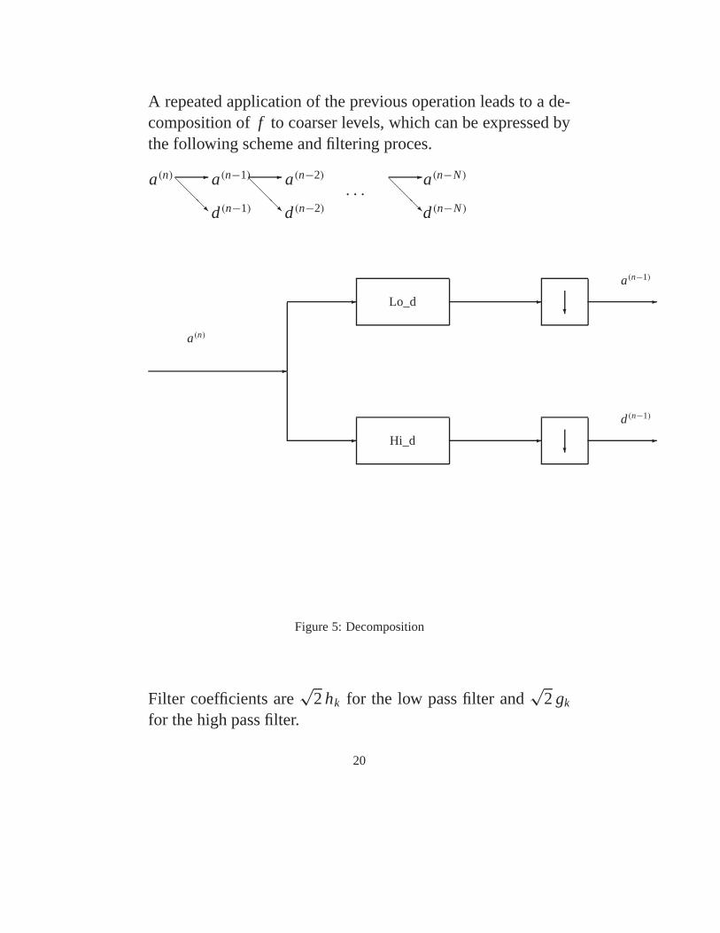
A repeated application of the previous operation leads to a de-composition of f to coarser levels, which can be expressed bythe following scheme and filtering proces.

a(n) ��

���

a(n−1)

d(n−1)

��

���

a(n−2)

d(n−2)

. . .�

��

��

a(n−N)

d(n−N)

�

�

�

Lo_d

Hi_d

a(n)

�

�

a(n−1)

d(n−1)

�

�

�

�

Figure 5: Decomposition

Filter coefficients are√

2 hk for the low pass filter and√

2 gk

for the high pass filter.

20

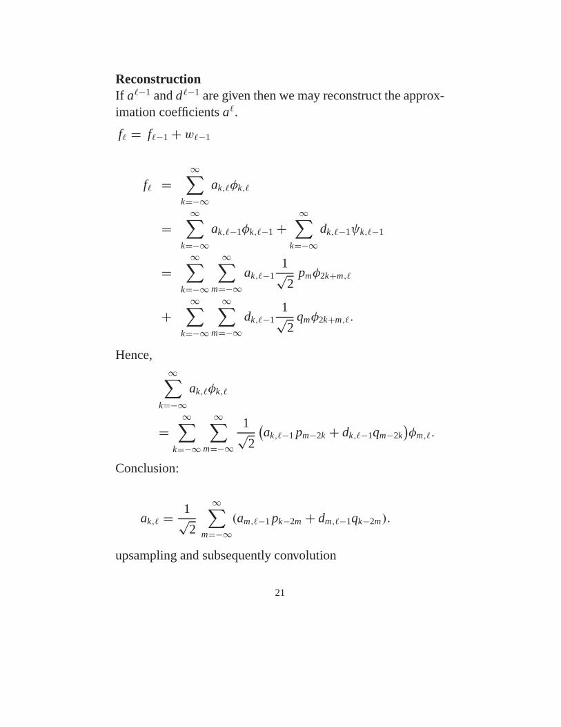
ReconstructionIf a�−1 and d�−1 are given then we may reconstruct the approx-imation coefficients a�.

f� = f�−1 + w�−1

f� =∞∑

k=−∞ak,�φk,�

=∞∑

k=−∞ak,�−1φk,�−1 +

∞∑k=−∞

dk,�−1ψk,�−1

=∞∑

k=−∞

∞∑m=−∞

ak,�−11√2

pmφ2k+m,�

+∞∑

k=−∞

∞∑m=−∞

dk,�−11√2

qmφ2k+m,�.

Hence,∞∑

k=−∞ak,�φk,�

=∞∑

k=−∞

∞∑m=−∞

1√2

(ak,�−1 pm−2k + dk,�−1qm−2k

)φm,�.

Conclusion:

ak,� = 1√2

∞∑m=−∞

(am,�−1 pk−2m + dm,�−1qk−2m).

upsampling and subsequently convolution

21

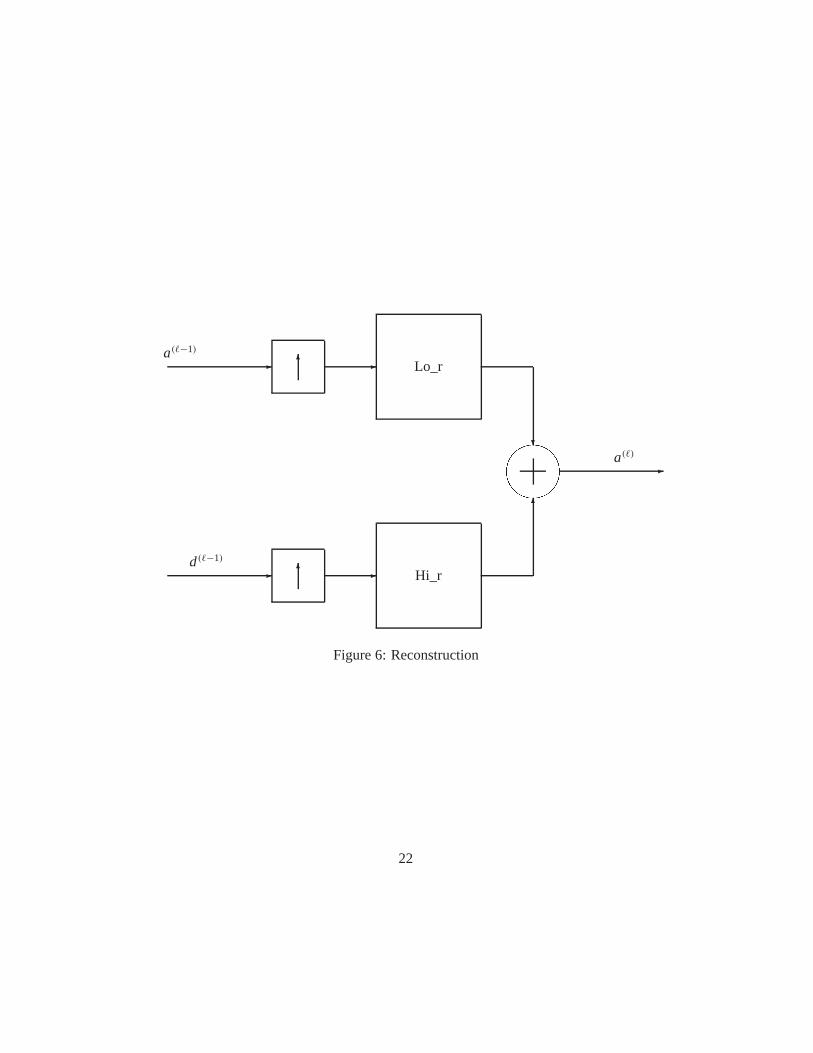
�a(�−1)

�d(�−1)

�

�

�

�

Lo_r

Hi_r

�

�����

�a(�)

Figure 6: Reconstruction

22

6. Examples

1. Haar wavelet

General characteristics:

OrthogonalSupport width 1Filters length 2Number of vanishing moments for ψ : 1Scaling function yes

0 0.1 0.2 0.3 0.4 0.5 0.6 0.7 0.8 0.9 1−1.5

−1

−0.5

0

0.5

1

1.5

Figure 7: Haar wavelet

23

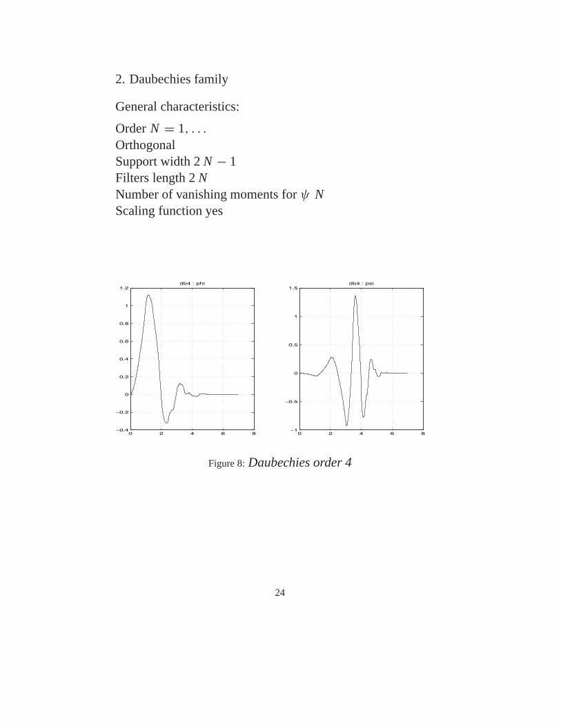
2. Daubechies family

General characteristics:

Order N = 1, . . .OrthogonalSupport width 2 N − 1Filters length 2 NNumber of vanishing moments for ψ NScaling function yes

0 2 4 6 8−0.4

−0.2

0

0.2

0.4

0.6

0.8

1

1.2db4 : phi

0 2 4 6 8−1

−0.5

0

0.5

1

1.5db4 : psi

Figure 8: Daubechies order 4

24

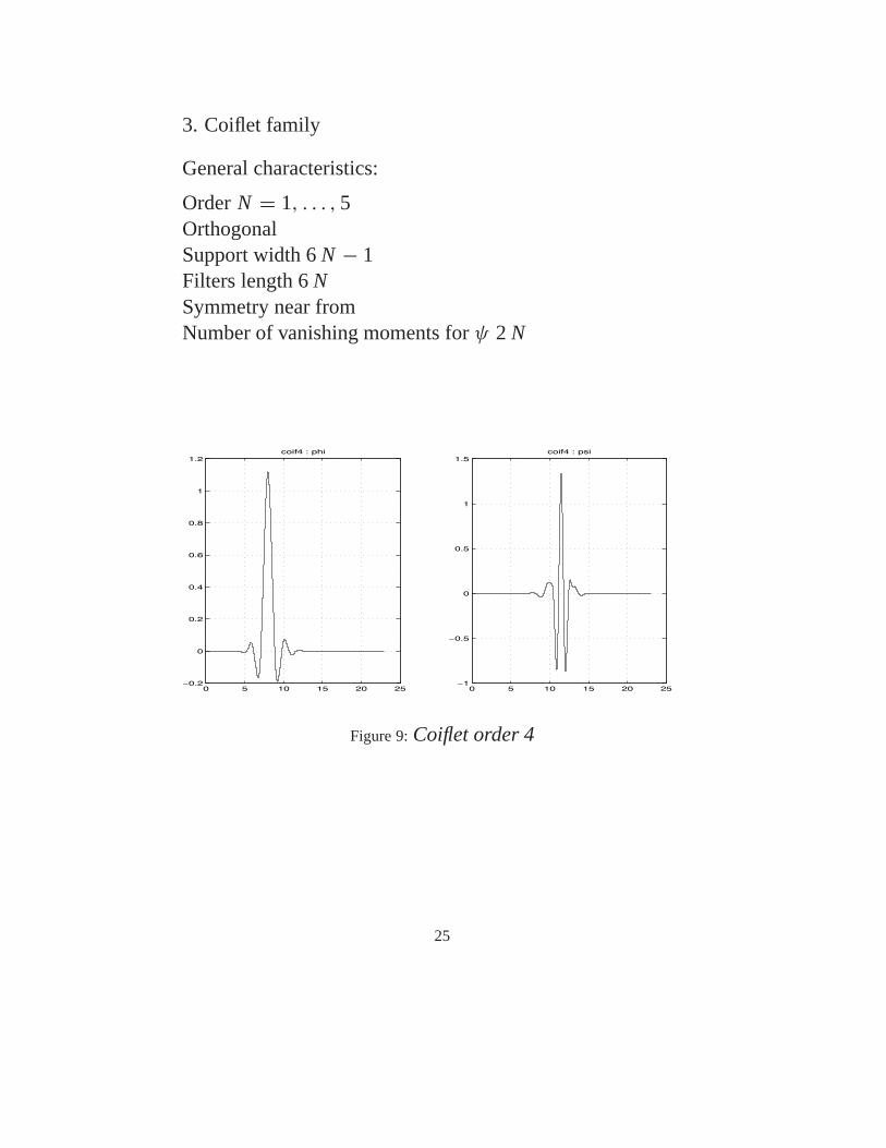
3. Coiflet family

General characteristics:

Order N = 1, . . . , 5OrthogonalSupport width 6 N − 1Filters length 6 NSymmetry near fromNumber of vanishing moments for ψ 2 N

0 5 10 15 20 25−0.2

0

0.2

0.4

0.6

0.8

1

1.2coif4 : phi

0 5 10 15 20 25−1

−0.5

0

0.5

1

1.5coif4 : psi

Figure 9: Coiflet order 4

25

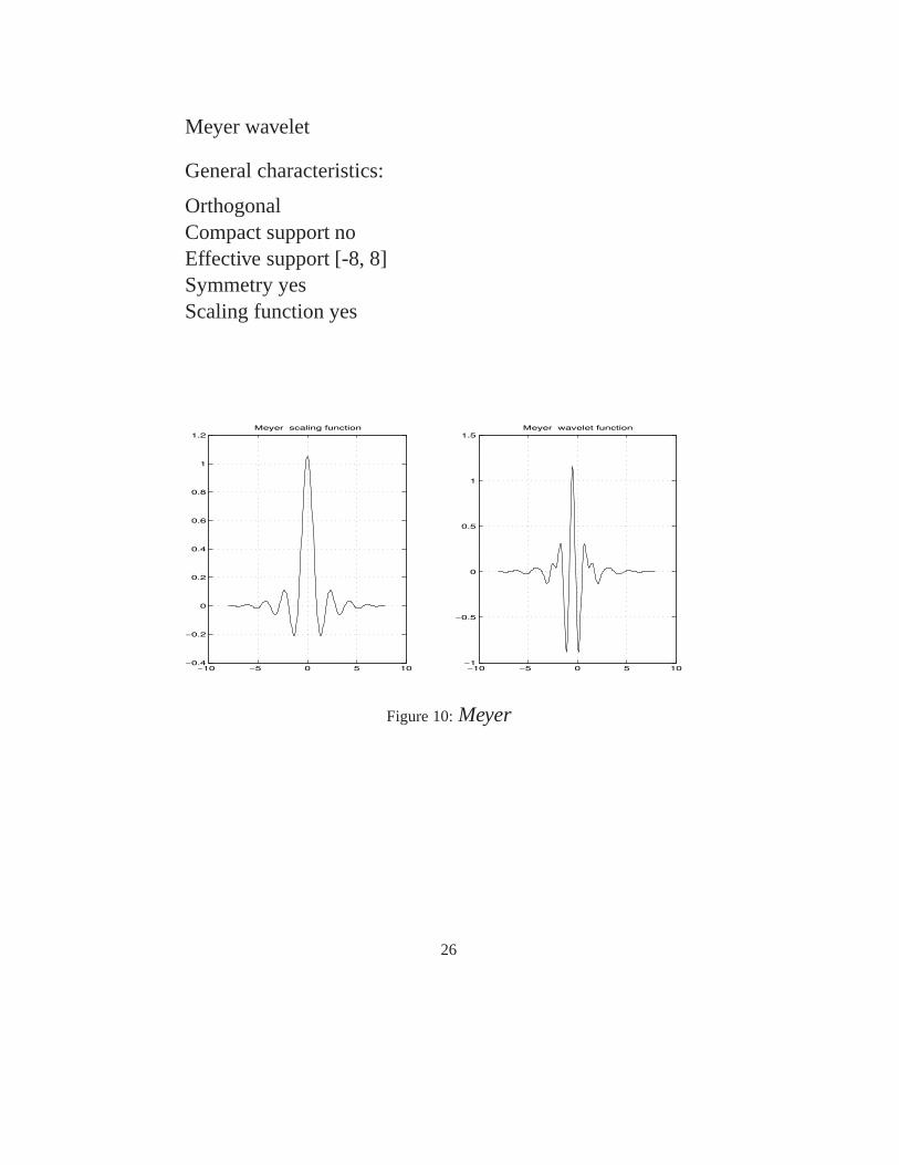
Meyer wavelet

General characteristics:

OrthogonalCompact support noEffective support [-8, 8]Symmetry yesScaling function yes

−10 −5 0 5 10−0.4

−0.2

0

0.2

0.4

0.6

0.8

1

1.2Meyer scaling function

−10 −5 0 5 10−1

−0.5

0

0.5

1

1.5Meyer wavelet function

Figure 10: Meyer

26