Waveguides - paginas.fe.up.ptmines/EE/EE_waveguides.pdf · MAPTele – EE Waveguides 2 Guided...
111
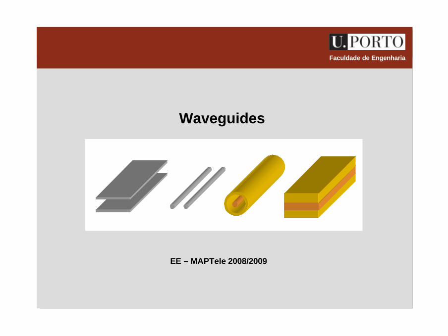
Faculdade de Engenharia Waveguides EE – MAPTele 2008/2009
Transcript of Waveguides - paginas.fe.up.ptmines/EE/EE_waveguides.pdf · MAPTele – EE Waveguides 2 Guided...
Faculdade de Engenharia
Waveguides
EE – MAPTele 2008/2009
MAPTele – EEWaveguides 2
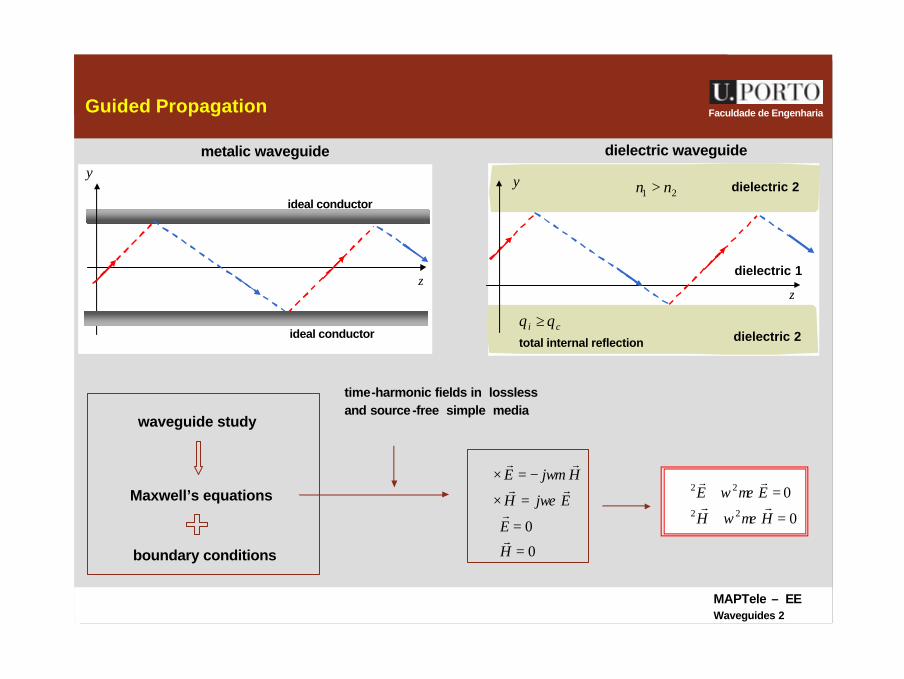
Faculdade de EngenhariaGuided Propagation
z
y
dielectric 2
dielectric 2
metalic waveguide
y
z
dielectric 1
dielectric waveguide
21 nn >
ci θθ ≥
waveguide study
Maxwell’s equations
boundary conditions 0
0
=⋅∇
=⋅∇
=×∇
−=×∇
H
E
EjH
HjE
r
r
rr
rr
ωε
ωµ
0
022
22
=+∇
=+∇
HH
EErr
rr
µεω
µεω
time-harmonic fields in losslessand source -free simple media
ideal conductor
ideal conductortotal internal reflection
MAPTele – EEWaveguides 3
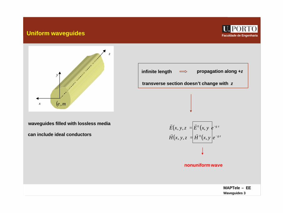
Faculdade de EngenhariaUniform waveguides
x
y
z
can include ideal conductors
propagation along +z
( )µε ,
transverse section doesn’t change with z
waveguides filled with lossless media
infinite length
( ) ( ) zeyxHzyxH γ−= ,,, 0rr
( ) ( ) zeyxEzyxE γ−= ,,, 0rr
nonuniform wave

MAPTele – EEWaveguides 4
Faculdade de EngenhariaUniform waveguides – field determination
x
y
z
( ) ( ) zeyxHzyxH γ−= ,,, 0rr
( ) ( ) zeyxEzyxE γ−= ,,, 0rr
0
022
22
=+∇
=+∇
HH
EErr
rr
µεω
µεω
0
00202
0202
=+∇
=+∇
HhH
EhE
xy
xyrr
rr
µεωγ 222 +=h
2
2
2
22
yxxy ∂∂
+∂∂
=∇
2 vector eqs. 6 scalar eqs.
00
00
00
02020202
02020202
02020202
=+∇=+∇
=+∇=+∇
=+∇=+∇
zzxyzzxy
yyxyyyxy
xxxyxxxy
HhHEhE
HhHEhE
HhHEhE
not all independent
MAPTele – EEWaveguides 5
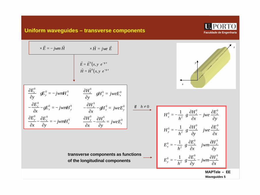
Faculdade de EngenhariaUniform waveguides – transverse components
x
y
z HjErr
ωµ−=×∇ EjHrr
ωε=×∇
000
000
000
zxy
yxz
xyz
Hjy
Ex
E
HjEx
E
HjEy
E
ωµ
ωµγ
ωµγ
−=∂
∂−∂
∂
−=−∂
∂−
−=+∂
∂
000
000
000
zxy
yxz
xyz
Ejy
Hx
H
EjHx
H
EjHy
H
ωε
ωεγ
ωεγ
=∂
∂−∂
∂
=−∂
∂−
=+∂
∂
( ) zeyxHH γ−= ,0rr
( ) zeyxEE γ−= ,0rr
∂
∂−∂
∂−=
∂
∂+∂
∂−=
∂
∂+∂
∂−=
∂
∂−∂
∂−=
xH
jy
Eh
E
yH
jx
Eh
E
xE
jy
Hh
H
yE
jx
Hh
H
zzy
zzx
zzy
zzx
00
20
00
20
00
20
00
20
1
1
1
1
ωµγ
ωµγ
ωεγ
ωεγ
transverse components as functionsof the longitudinal components
if 0≠h
MAPTele – EEWaveguides 6
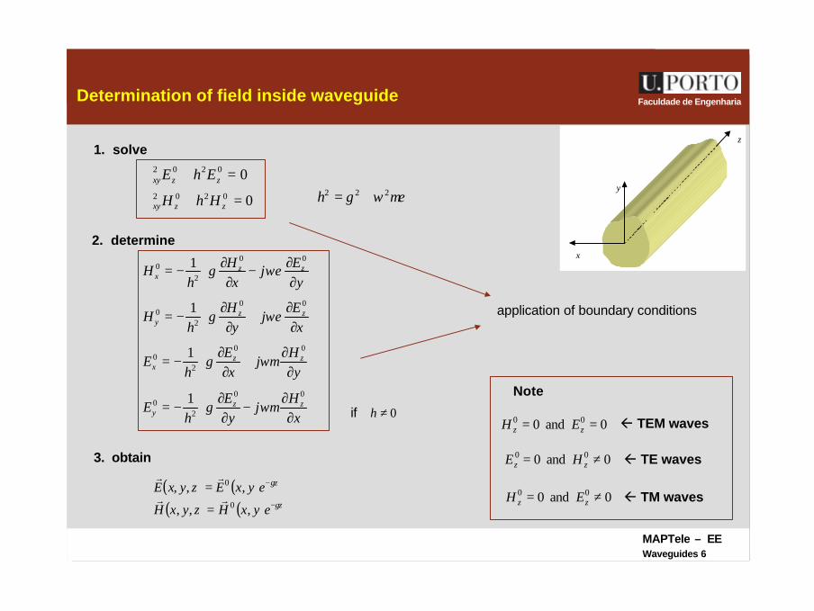
Faculdade de EngenhariaDetermination of field inside waveguide
x
y
z
∂
∂−
∂∂
−=
∂
∂+
∂∂
−=
∂
∂+
∂∂
−=
∂
∂−∂
∂−=
xH
jy
Eh
E
yH
jx
Eh
E
xE
jy
Hh
H
yEj
xH
hH
zzy
zzx
zzy
zzx
00
20
00
20
00
20
00
20
1
1
1
1
ωµγ
ωµγ
ωεγ
ωεγ
if 0≠h
2. determine
0
00202
0202
=+∇
=+∇
zzxy
zzxy
HhH
EhEµεωγ 222 +=h
1. solve
3. obtain
( ) ( )( ) ( ) z
z
eyxHzyxH
eyxEzyxEγ
γ
−
−
=
=
,,,
,,,0
0
rr
rr
application of boundary conditions
Note
ß TE waves
ß TEM waves
ß TM waves
0and0 00 ≠= zz HE
0and0 00 ≠= zz EH
0and0 00 == zz EH
MAPTele – EEWaveguides 7
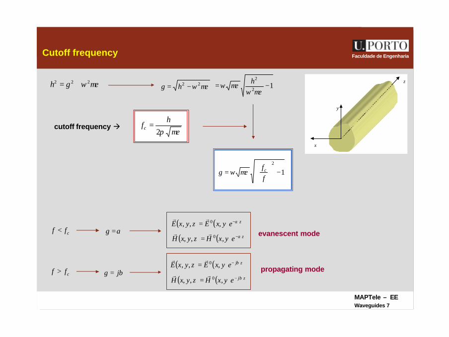
Faculdade de EngenhariaCutoff frequency
x
y
z µεωγ 222 +=h
cutoff frequency à
12
2
−=µεω
µεω hµεωγ 22 −= h
µεπ2
hfc =
12
−
=
ffcµεωγ
evanescent mode cff < αγ =( ) ( ) zeyxHzyxH α−= ,,, 0
rr( ) ( ) zeyxEzyxE α−= ,,, 0
rr
propagating mode cff > βγ j=
( ) ( ) zjeyxHzyxH β−= ,,, 0rr
( ) ( ) zjeyxEzyxE β−= ,,, 0rr
MAPTele – EEWaveguides 8
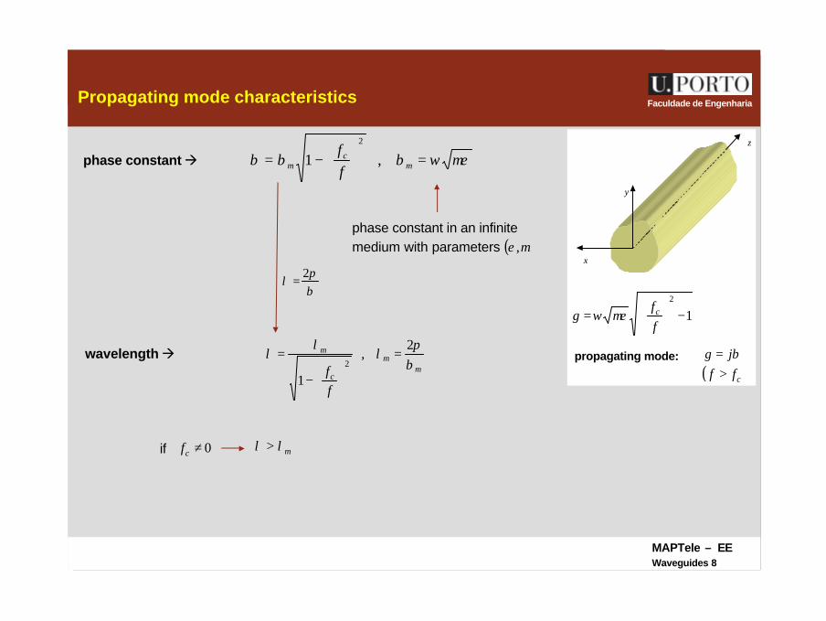
Faculdade de EngenhariaPropagating mode characteristics
x
y
z
( )cff >βγ j=
12
−
=
ffcµεωγ
propagating mode:
phase constant à µεωβββ =
−= m
cm f
f,1
2
wavelength àm
m
c
m
ff β
πλ
λλ
2,
12
=
−
=
βπ
λ2
=
if 0≠cf mλλ >
phase constant in an infinitemedium with parameters ( )µε ,
MAPTele – EEWaveguides 9
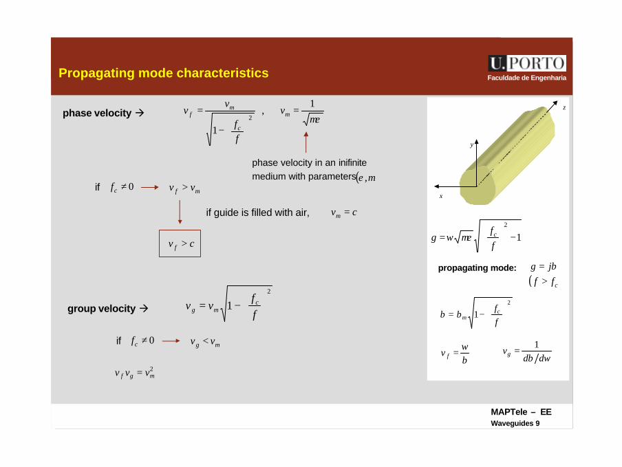
Faculdade de EngenhariaPropagating mode characteristics
x
y
z
( )cff >βγ j=
12
−
=
ffcµεωγ
propagating mode:
phase velocity à
2
1
−=
ffc
mββgroup velocity à
βω
=fv
if 0≠cf mf vv >
phase velocity in an inifinitemedium with parameters ( )µε ,
µε1
,
12
=
−
= m
c
mf v
ff
vv
if guide is filled with air, cvm =
cv f >
2
1
−=
ff
vv cmg
if 0≠cf mg vv <
ωβ ddvg
1=
2mgf vvv =
MAPTele – EEWaveguides 10
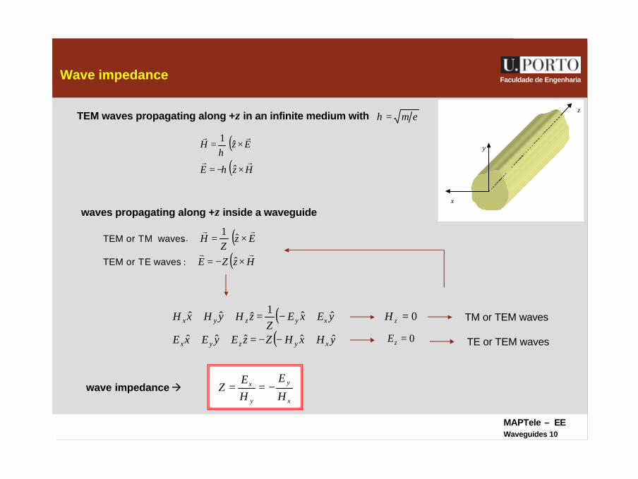
Faculdade de EngenhariaWave impedance
x
y
z TEM waves propagating along +z in an infinite medium with
( )( )HzE
EzH
rr
rr
×−=
×=
ˆ
ˆ1
η
η
εµη =
waves propagating along +z inside a waveguide
( )( )HzZE
EzZ
Hrr
rr
×−=
×=
ˆ
ˆ1
:wavesTEorTEM
waves TMorTEM :
( )( )yHxHZzEyExE
yExEZ
zHyHxH
xyzyx
xyzyx
ˆˆˆˆˆ
ˆˆ1ˆˆˆ
+−−=++
+−=++ 0=zH
0=zE
TM or TEM waves
TE or TEM waves
wave impedance àx
y
y
x
H
E
HE
Z −==
MAPTele – EEWaveguides 11
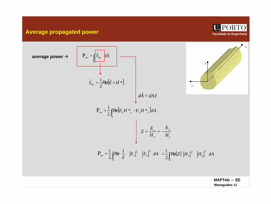
Faculdade de EngenhariaAverage propagated power
x
y
z
average power à
x
y
y
x
H
E
HE
Z −==
∫ ⋅=A
avav AdSrr
P
zdAAd ˆ=r
{ }*21
HESav
rrr×= Re
{ }∫ −=A
xyyxav dAHEHE **21P Re
∫
+
=
Ayxav dAEE
Z
22121P Re { }∫
+=
Ayx dAHHZ
22
21
Re
MAPTele – EEWaveguides 12
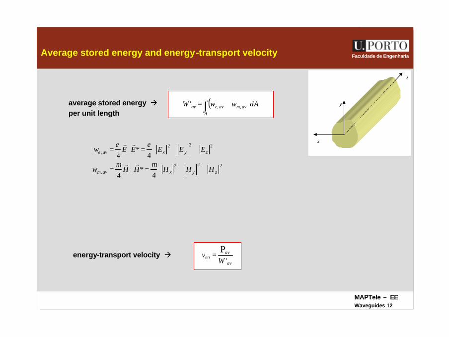
Faculdade de EngenhariaAverage stored energy and energy-transport velocity
x
y
z
average stored energy àper unit length
( )∫ +=A
avmaveav dAwwW ,,'
++=⋅= 222
, 4*
4 zyxave EEEEEwεε rr
++=⋅= 222
, 4*
4 zyxavm HHHHHwµµ rr
av
aven W
v'
P=energy-transport velocity à
MAPTele – EEWaveguides 13
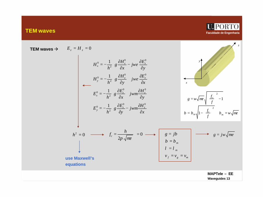
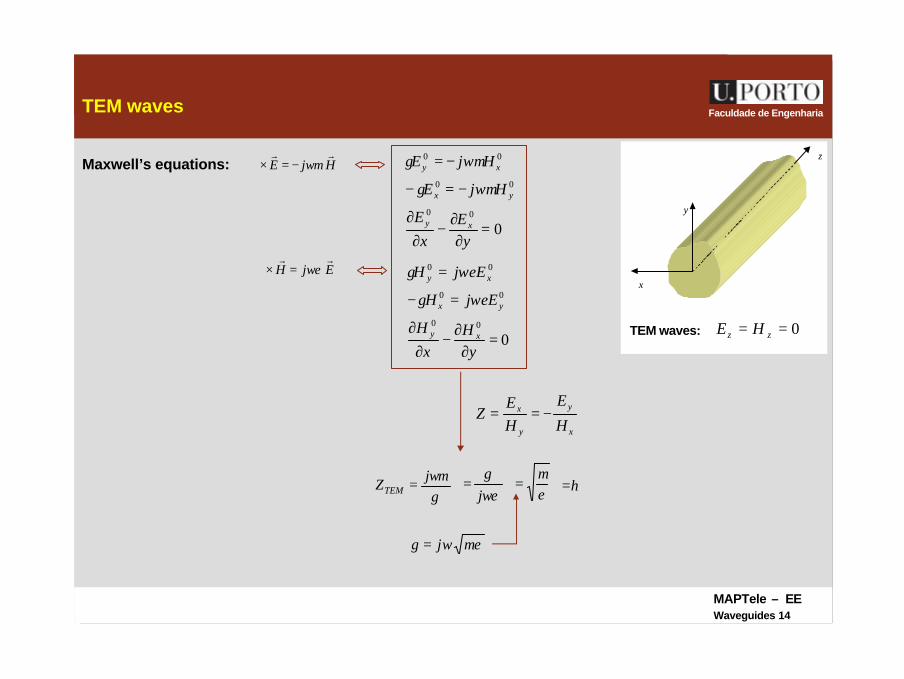
Faculdade de EngenhariaTEM waves
x
y
z TEM waves à 0== zz HE
∂
∂−∂
∂−=
∂
∂+
∂∂
−=
∂
∂+
∂∂
−=
∂
∂−
∂∂
−=
xHj
yE
hE
yH
jx
Eh
E
xE
jy
Hh
H
yE
jx
Hh
H
zzy
zzx
zzy
zzx
00
20
00
20
00
20
00
20
1
1
1
1
ωµγ
ωµγ
ωεγ
ωεγ
02 =hµεπ2
hfc =
mgf
m
m
vvv
j
==
=
=
=
λλ
ββ
βγ
12
−
=
ffcµεωγ
2
1
−=
ffc
mββ
use Maxwell’s equations
εµωγ j=
µεωβ =m
0=
MAPTele – EEWaveguides 14
Faculdade de EngenhariaTEM waves
x
y
z
TEM waves: 0== zz HE
Maxwell’s equations:
000
00
00
=∂
∂−
∂∂
−=−
−=
yE
x
E
HjE
HjE
xy
yx
xy
ωµγ
ωµγ
000
00
00
=∂
∂−
∂∂
=−
=
yH
x
H
EjH
EjH
xy
yx
xy
ωεγ
ωεγ
HjErr
ωµ−=×∇
EjHrr
ωε=×∇
γωµjZTEM =
x
y
y
x
H
E
HE
Z −==
ωεγ
j=
εµ
= η=
εµωγ j=
MAPTele – EEWaveguides 15
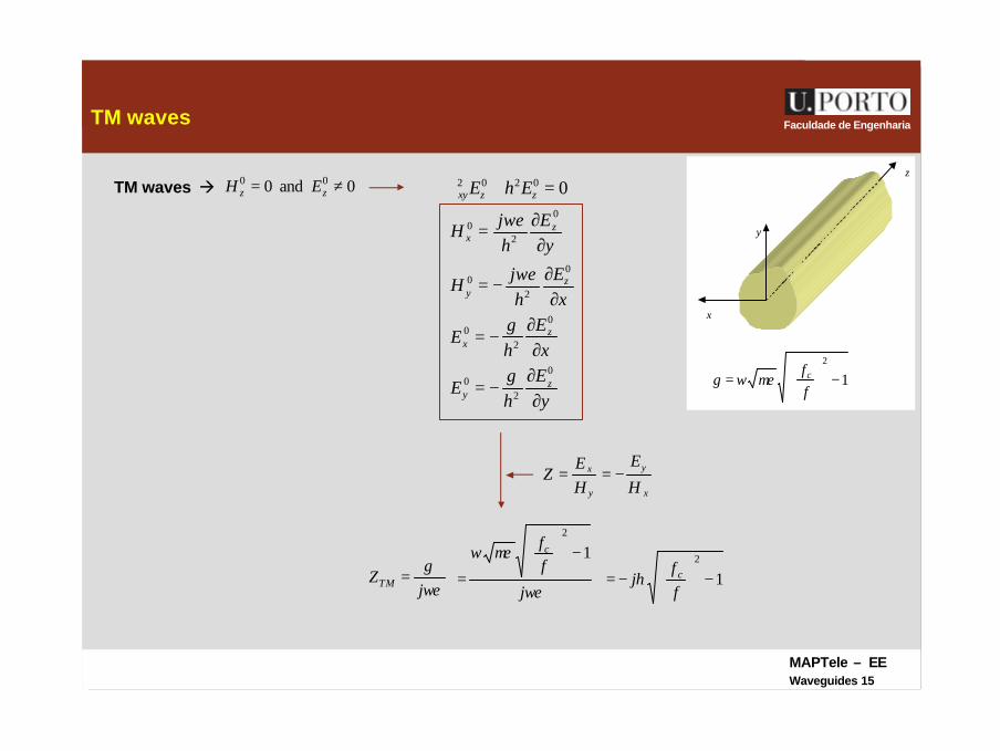
Faculdade de EngenhariaTM waves
x
y
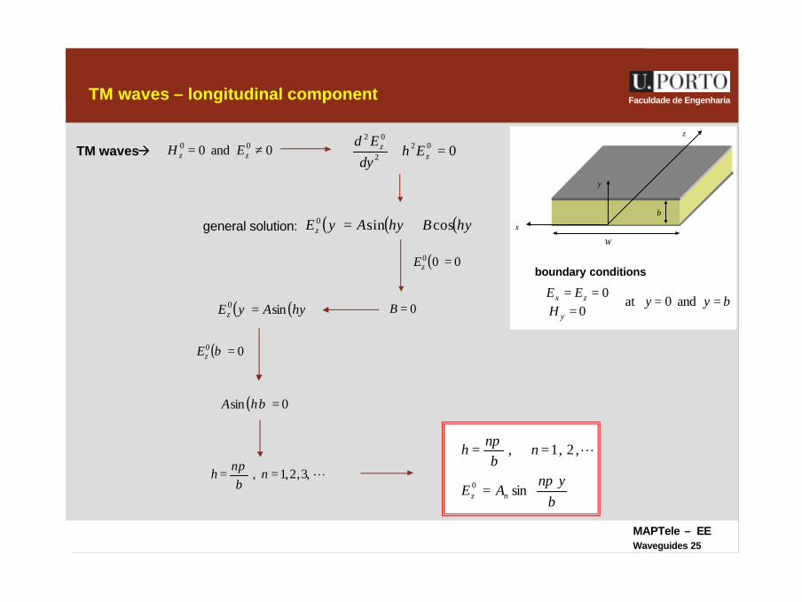
z TM waves à 0and0 00 ≠= zz EH 00202 =+∇ zzxy EhE
yE
hE
xE
hE
xE
hj
H
yE
hj
H
zy
zx
zy
zx
∂∂
−=
∂∂
−=
∂∂−=
∂∂=
0
20
0
20
0
20
0
20
γ
γ
ωε
ωε
x
y
y
x
H
E
HE
Z −==
ωεγ
jZTM =
ωε
µεω
j
ffc 1
2
−
= 12
−
−=
ff
j cη
12
−
=
ffcµεωγ
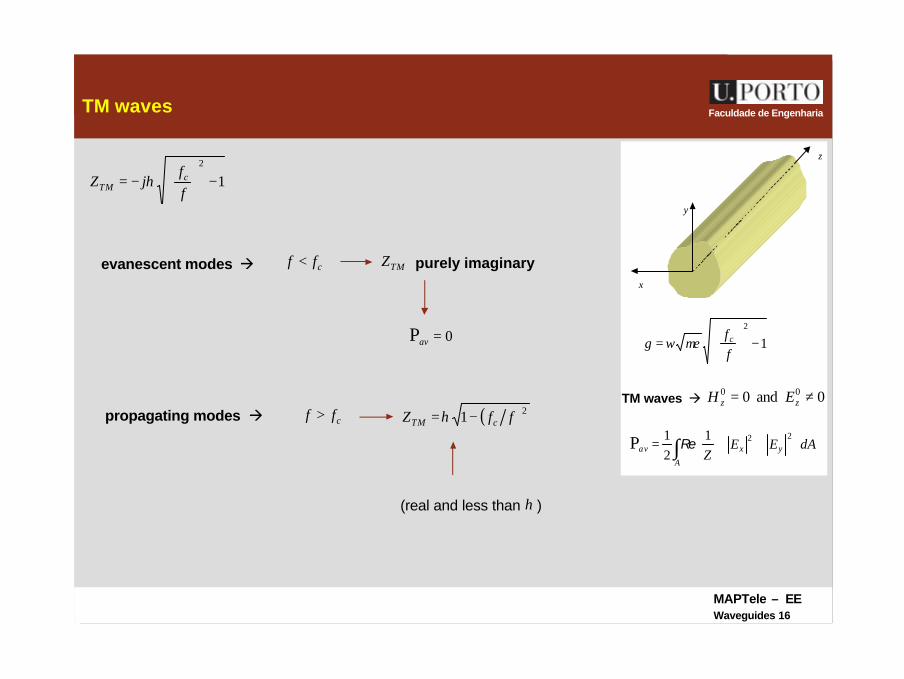
MAPTele – EEWaveguides 16
Faculdade de EngenhariaTM waves
x
y
z
TM waves à 0and0 00 ≠= zz EH
12
−
−=
ff
jZ cTM η
12
−
=
ffcµεωγ
∫
+
=
A
yxav dAEEZ
22121P Re
evanescent modes à cff <
cff >propagating modes à
TMZ purely imaginary
0P =av
( )21 ffZ cTM −=η
(real and less than )η
MAPTele – EEWaveguides 17
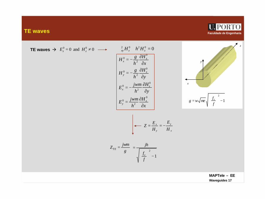
Faculdade de EngenhariaTE waves
x
y
z TE waves à 0and0 00 ≠= zz HE
x
y
y
x
H
E
HE
Z −==
12
−
=
ffcµεωγ
00202 =+∇ zzxy HhH
xH
hj
E
yH
hj
E
yH
hH
xH
hH
zy
zx
zy
zx
∂∂=
∂∂
−=
∂∂−=
∂∂−=
0
20
0
20
0
20
0
20
ωµ
ωµ
γ
γ
γωµj
ZTE =
12
−
=
ff
j
c
η

MAPTele – EEWaveguides 18
Faculdade de EngenhariaTE waves
x
y
z
TE waves à 0and0 00 ≠= zz HE
12
−
=
ffcµεωγ
∫
+
=
A
yxav dAEEZ
22121P Re
evanescent modes à cff <
cff >propagating modes à
TEZ purely imaginary
0P =av
(real and larger than )η
12
−
=
ff
jZ
c
TEη
( )21 ffZ cTE −=η
MAPTele – EEWaveguides 19
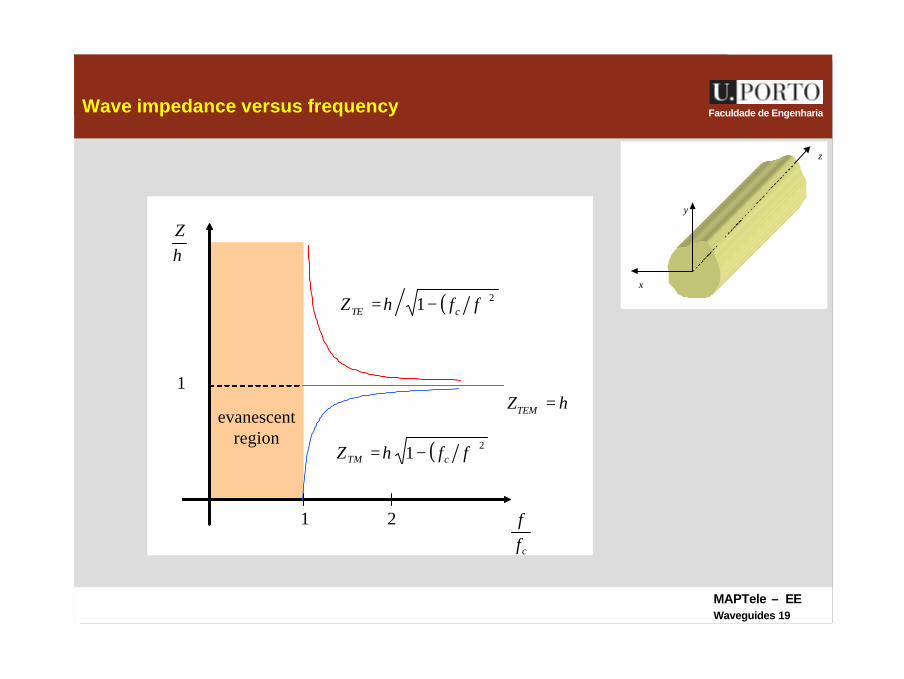
Faculdade de EngenhariaWave impedance versus frequency
x
y
z
1
ηZ
evanescent region
cff
2 1
( )21 ffZ cTE −= η
( )21 ffZ cTM −= η
η=TEMZ
MAPTele – EEWaveguides 20
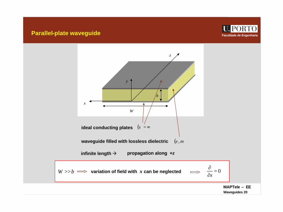
Faculdade de EngenhariaParallel-plate waveguide
waveguide filled with lossless dielectric
b
y
z
x
W
( )µε ,
ideal conducting plates ( )∞=σ
infinite length à propagation along +z
bW >> 0=∂∂x
variation of field with x can be neglected
MAPTele – EEWaveguides 21
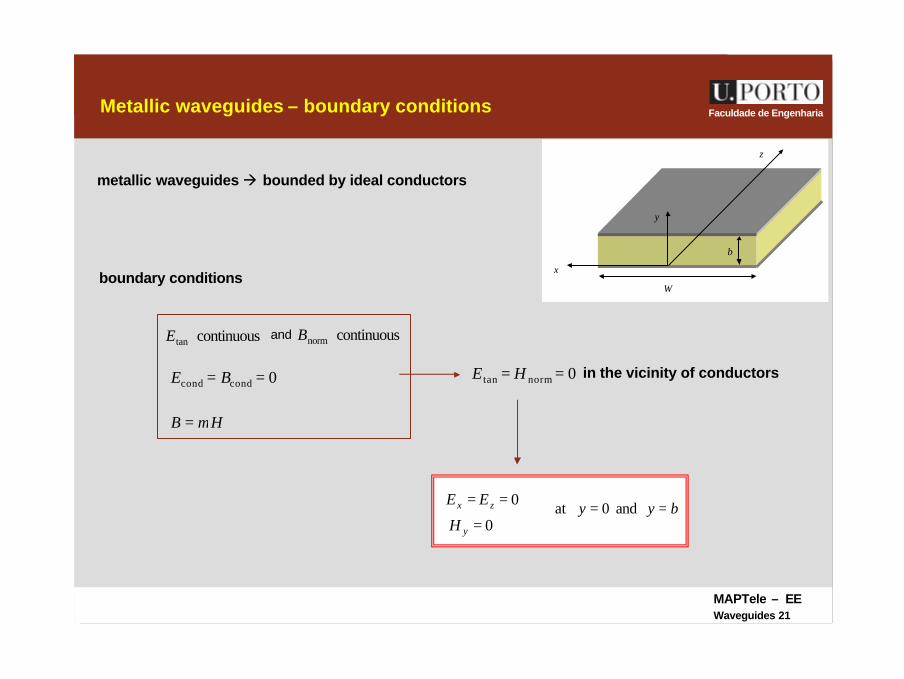
Faculdade de EngenhariaMetallic waveguides – boundary conditions
metallic waveguides à bounded by ideal conductors
0condcond == BE
continuoustanE continuousnormBand
boundary conditions
HB µ=
0normtan == HE in the vicinity of conductors
b
y
z
x
W
0== zx EE
0=yHbyy == and0at
MAPTele – EEWaveguides 22
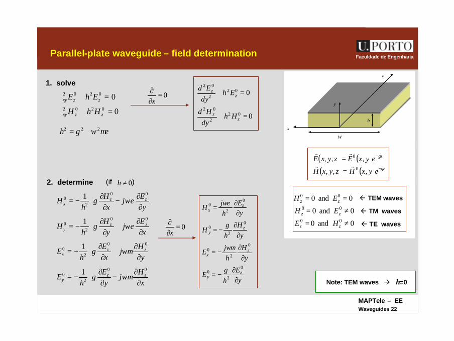
Faculdade de EngenhariaParallel-plate waveguide – field determination
b
y
z
x
W
∂
∂−
∂∂
−=
∂
∂+
∂∂
−=
∂
∂+
∂∂
−=
∂
∂−∂
∂−=
xH
jy
Eh
E
yH
jx
Eh
E
xE
jy
Hh
H
yEj
xH
hH
zzy
zzx
zzy
zzx
00
20
00
20
00
20
00
20
1
1
1
1
ωµγ
ωµγ
ωεγ
ωεγ
(if )0≠h2. determine
0
00202
0202
=+∇
=+∇
zzxy
zzxy
HhH
EhE
µεωγ 222 +=h
1. solve
0=∂∂x
0
0
022
02
022
02
=+
=+
zz
zz
Hhdy
Hd
Ehdy
Ed
yE
hE
yH
hj
E
yH
hH
yE
hj
H
zy
zx
zy
zx
∂∂
−=
∂∂
−=
∂∂
−=
∂∂
=
0
20
0
20
0
20
0
20
γ
ωµ
γ
ωε
ß TE waves
ß TEM waves
ß TM waves
0and0 00 ≠= zz HE
0and0 00 ≠= zz EH
0and0 00 == zz EH
( ) ( )( ) ( ) z
z
eyxHzyxH
eyxEzyxEγ
γ
−
−
=
=
,,,
,,,0
0
rr
rr
0=∂∂x
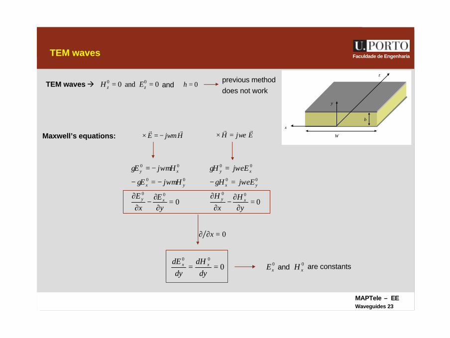
Note: TEM waves à h=0
MAPTele – EEWaveguides 23
Faculdade de EngenhariaTEM waves
b
y
z
x
W
TEM waves à 0and0 00 == zz EH
Maxwell’s equations:
000
00
00
=∂
∂−
∂∂
−=−
−=
yE
x
E
HjE
HjE
xy
yx
xy
ωµγ
ωµγ
000
00
00
=∂
∂−
∂∂
=−
=
yH
x
H
EjH
EjH
xy
yx
xy
ωεγ
ωεγ
HjErr
ωµ−=×∇ EjHrr
ωε=×∇
and 0=hprevious method does not work
0=∂∂ x
000
==dy
dHdy
dE xx 0xE 0
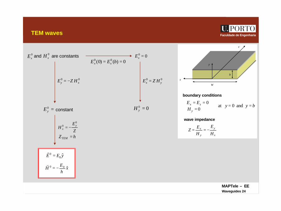
xHand are constants
MAPTele – EEWaveguides 24
Faculdade de EngenhariaTEM waves
b
y
z
x
W
0xE 0
xHand are constants0)()0( 00 == bEE xx
00yx HZE =
00 =yH
00xy HZE −=
=0yE
η=TEMZ
constant
00 =xE
yEE ˆ00 =
r
boundary conditions
0== zx EE0=yH
byy == and0at
wave impedance
x
y
y
x
H
E
HE
Z −==
xEH ˆ00
η−=
r
Z
EH y
x
00 −=
MAPTele – EEWaveguides 25
Faculdade de EngenhariaTM waves – longitudinal component
b
y
z
x
W
general solution:
0and0 00 ≠= zz EH 0022
02
=+ zz Eh
dyEd
( ) ( ) ( )hyBhyAyEz cossin0 +=
( ) 000 =zE
0=B
L,3,2,1, == nb
nh
π
( ) 0sin =bhA
=
==
byn
AE
nb
nh
nz
π
π
sin
,2,1,
0
L
TM wavesà
boundary conditions
0== zx EE0=yH
byy == and0at
( ) 00 =bEz
( ) ( )hyAyEz sin0 =
MAPTele – EEWaveguides 26
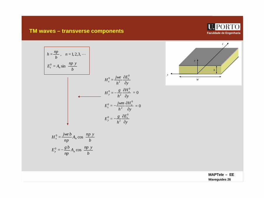
Faculdade de EngenhariaTM waves – transverse components
b
y
z
x
W
=
==
byn
AE
nb
nh
nzπ
π
sin
,3,2,1,
0
L
yE
hE
yH
hj
E
yH
hH
yE
hj
H
zy
zx
zy
zx
∂∂
−=
∂∂
−=
∂∂
−=
∂∂
=
0
20
0
20
0
20
0
20
γ
ωµ
γ
ωε
−=
=
bynA
nbE
byn
An
bjH
ny
nx
ππ
γ
ππ
ωε
cos
cos
0
0
0=
0=
MAPTele – EEWaveguides 27
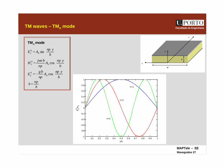
Faculdade de EngenhariaTM waves – TMn mode
b
y
z
x
W
TMn mode
−=
=
=
byn
An
bE
byn
An
bjH
byn
AE
ny
nx
nz
ππ
γ
ππ
ωε
π
cos
cos
sin
0
0
0
bn
hπ=
0 0.1 0.2 0.3 0.4 0.5 0.6 0.7 0.8 0.9 1-1
-0.8
-0.6
-0.4
-0.2
0
0.2
0.4
0.6
0.8
1
y/b
Ez0 /A
n
n=1
n=2
n=3
MAPTele – EEWaveguides 28
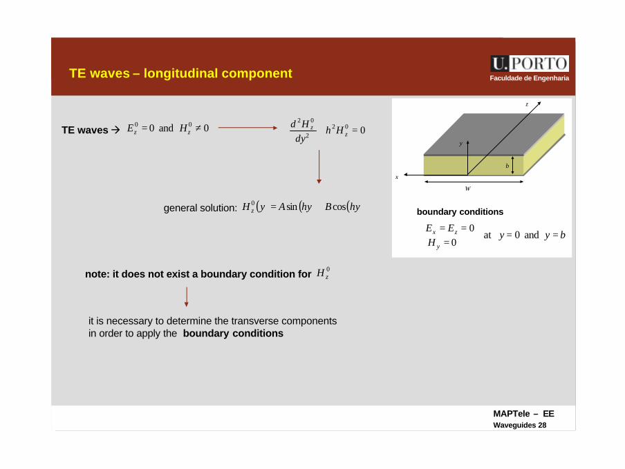
Faculdade de EngenhariaTE waves – longitudinal component
b
y
z
x
W
TE waves à 0and0 00 ≠= zz HE 0022
02
=+ zz Hh
dyHd
( ) ( ) ( )hyBhyAyH z cossin0 +=
note: it does not exist a boundary condition for 0zH
it is necessary to determine the transverse components in order to apply the boundary conditions
boundary conditions
0== zx EE0=yH
byy == and0at
general solution:
MAPTele – EEWaveguides 29
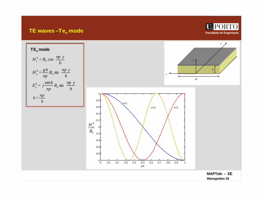
Faculdade de EngenhariaTE waves –Ten mode
b
y
z
x
W
=
=
=
byn
Bn
bjE
bynB
nbH
bynBH
nx
ny
nz
ππ
ωµ
ππ
γ
π
sin
sin
cos
0
0
0
TEn mode
bn
hπ=
0 0.1 0.2 0.3 0.4 0.5 0.6 0.7 0.8 0.9 1-1
-0.8
-0.6
-0.4
-0.2
0
0.2
0.4
0.6
0.8
1
y/b
Ez0 /A
n
n=1
n=2n=3
n
z
BH 0
MAPTele – EEWaveguides 30
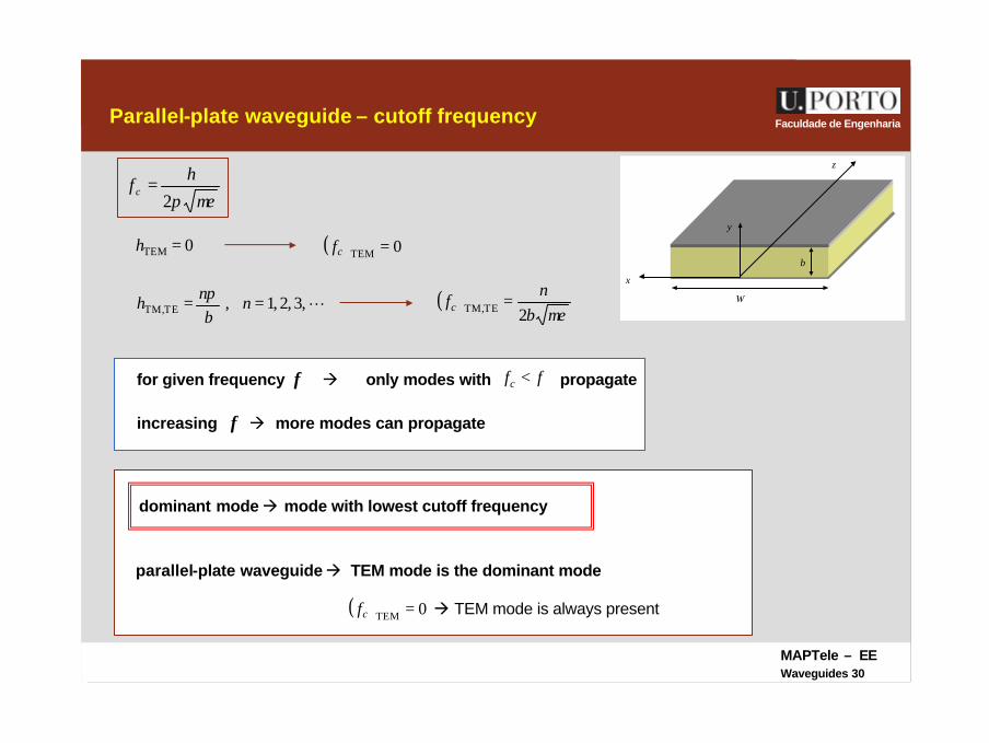
Faculdade de EngenhariaParallel-plate waveguide – cutoff frequency
b
y
z
x
W
µεπ2
hf c =
0TEM =h
L,3,2,1,TETM, == nb
nh π
( ) 0TEM =cf
( )µεb
nfc 2TETM, =
dominant mode à mode with lowest cutoff frequency
parallel-plate waveguide à TEM mode is the dominant mode
for given frequency f à only modes with propagate ffc <
à TEM mode is always present( ) 0TEM =cf
increasing f à more modes can propagate
MAPTele – EEWaveguides 31
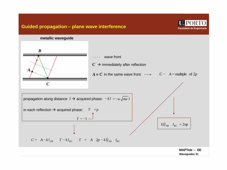
Faculdade de EngenhariaGuided propagation – plane wave interference
metallic waveguide
A
B
C
wave front
C à immediately after reflection
A e C in the same wave front π2ofmultiple=∠−∠ AC
Γ∠+−Γ∠+−∠=∠ BCAB lklkAC
propagation along distance là acquired phase:
in each reflection à acquired phase: Γ∠ π=
1−=Γ
( )BCAB llkA +−+∠= π2
( ) πnllk BCAB 2=+
lk− lεµω−=
MAPTele – EEWaveguides 32
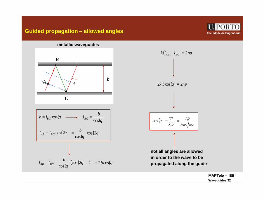
Faculdade de EngenhariaGuided propagation – allowed angles
metallic waveguides
A
B
C
( )θcosBClb =
b
( ) πnllk BCAB 2=+
θ
( )θcosb
lBC =
( )θ2cosBCAB ll =( ) ( )θθ
2coscos
b=
( ) ( )( )12coscos
+=+ θθ
bll BCAB ( )θcos2b=
( ) πθ nbk 2cos2 =
( )bk
nπθ =cos
εµωπ
bn
=
not all angles are allowed in order to the wave to be propagated along the guide
MAPTele – EEWaveguides 33
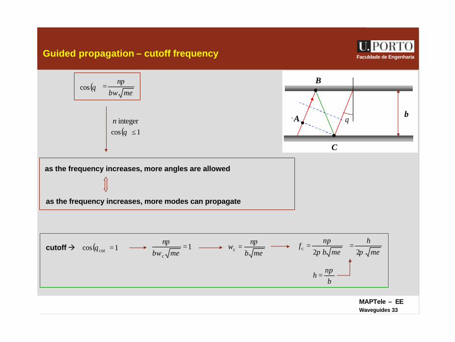
Faculdade de EngenhariaGuided propagation – cutoff frequency
A
B
C
bθ
( )θcosεµω
πb
n=
integern( ) 1cos ≤θ
as the frequency increases, more angles are allowed
as the frequency increases, more modes can propagate
cutoff à ( ) 1cos cut =θ 1c
=εµω
πb
nεµ
πω
bn
=c εµππ
bn
f2c =
bn
hπ
=
εµπ2h
=
MAPTele – EEWaveguides 34
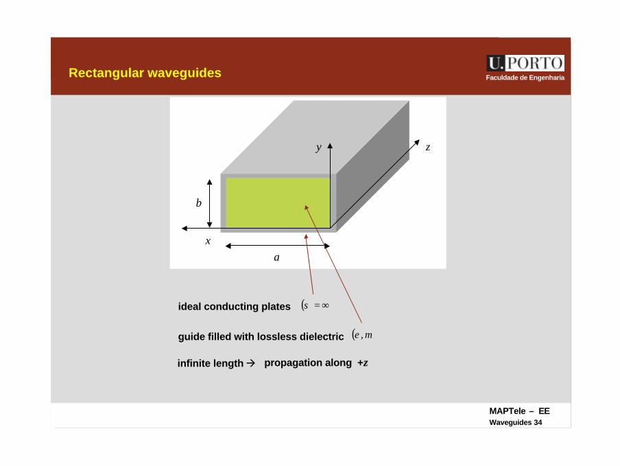
Faculdade de EngenhariaRectangular waveguides
guide filled with lossless dielectric ( )µε ,
ideal conducting plates ( )∞=σ
infinite length à propagation along +z
b
y z
x a
MAPTele – EEWaveguides 35
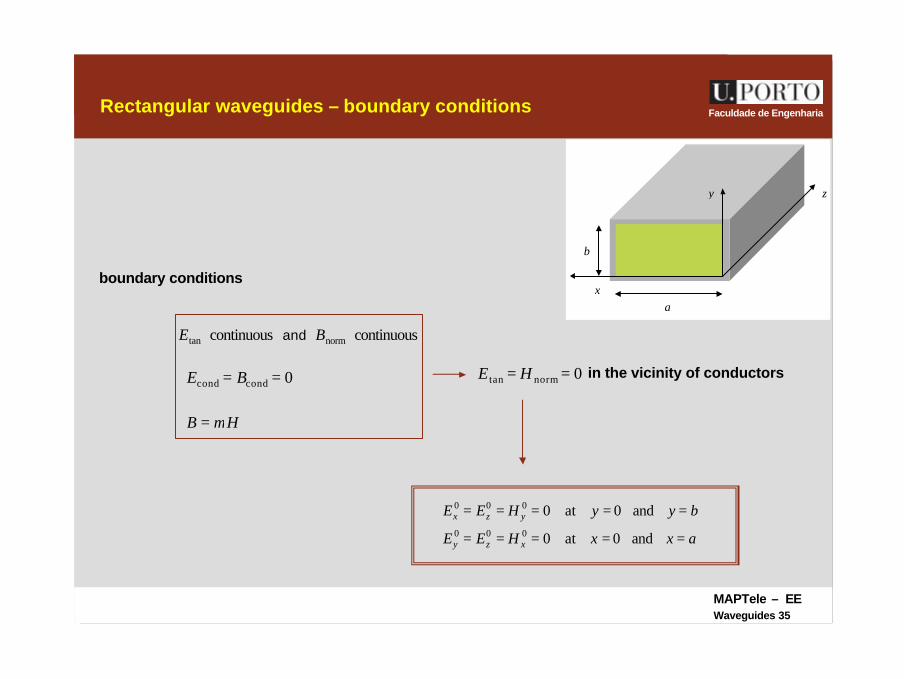
Faculdade de EngenhariaRectangular waveguides – boundary conditions
0condcond == BE
continuoustanE continuousnormBand
boundary conditions
HB µ=
0normtan == HE in the vicinity of conductors
b
y z
x a
axxHEE
byyHEE
xzy
yzx
=====
=====
and0at0
and0at0000
000
MAPTele – EEWaveguides 36
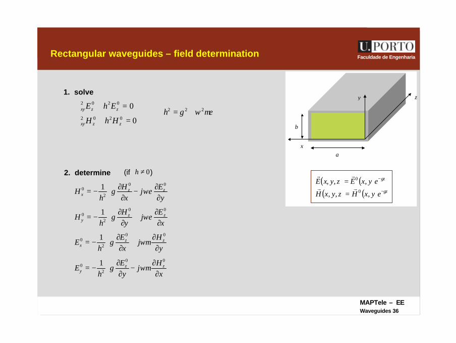
Faculdade de EngenhariaRectangular waveguides – field determination
∂
∂−
∂∂
−=
∂
∂+
∂∂
−=
∂
∂+
∂∂
−=
∂
∂−∂
∂−=
xH
jy
Eh
E
yH
jx
Eh
E
xE
jy
Hh
H
yEj
xH
hH
zzy
zzx
zzy
zzx
00
20
00
20
00
20
00
20
1
1
1
1
ωµγ
ωµγ
ωεγ
ωεγ
(if )0≠h2. determine
0
00202
0202
=+∇
=+∇
zzxy
zzxy
HhH
EhEµεωγ 222 +=h
1. solve
( ) ( )( ) ( ) z
z
eyxHzyxH
eyxEzyxEγ
γ
−
−
=
=
,,,
,,,0
0
rr
rr
b
y z
x a
MAPTele – EEWaveguides 37
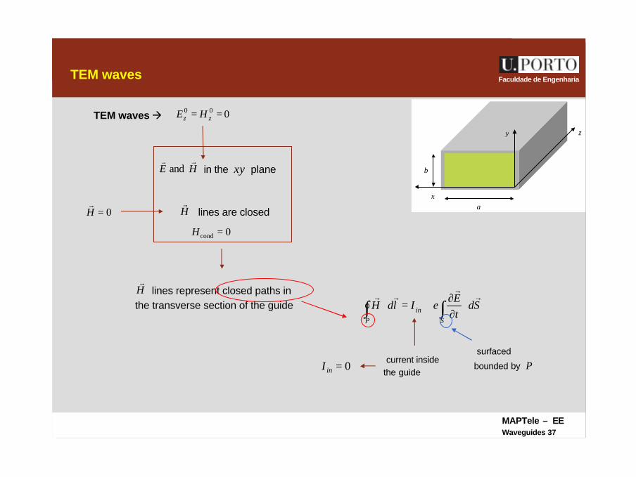
Faculdade de EngenhariaTEM waves
TEM waves à
b
y z
x a
000 == zz HE
HErr
and in the xy plane
∫∫ ⋅∂∂
+=⋅S
inP
SdtE
IldHr
rrr
ε
0=⋅∇ Hr
Hr
lines represent closed paths in the transverse section of the guide
0cond =H
lines are closedHr
current inside the guide
surfaced
bounded by P0=inI
MAPTele – EEWaveguides 38
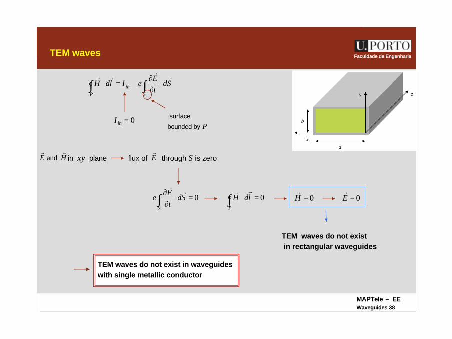
Faculdade de EngenhariaTEM waves
TEM waves do not existin rectangular waveguides
b
y z
x a
HErr
and in xy plane
∫∫ ⋅∂∂
+=⋅S
inP
SdtE
IldHr
rrr
ε
surface
bounded by P0=inI
flux of through S is zeroEr
0=⋅∂∂
∫S
SdtE rr
ε 0=⋅∫P
ldHrr
0=Hr
0=Er
TEM waves do not exist in waveguides with single metallic conductor
MAPTele – EEWaveguides 39
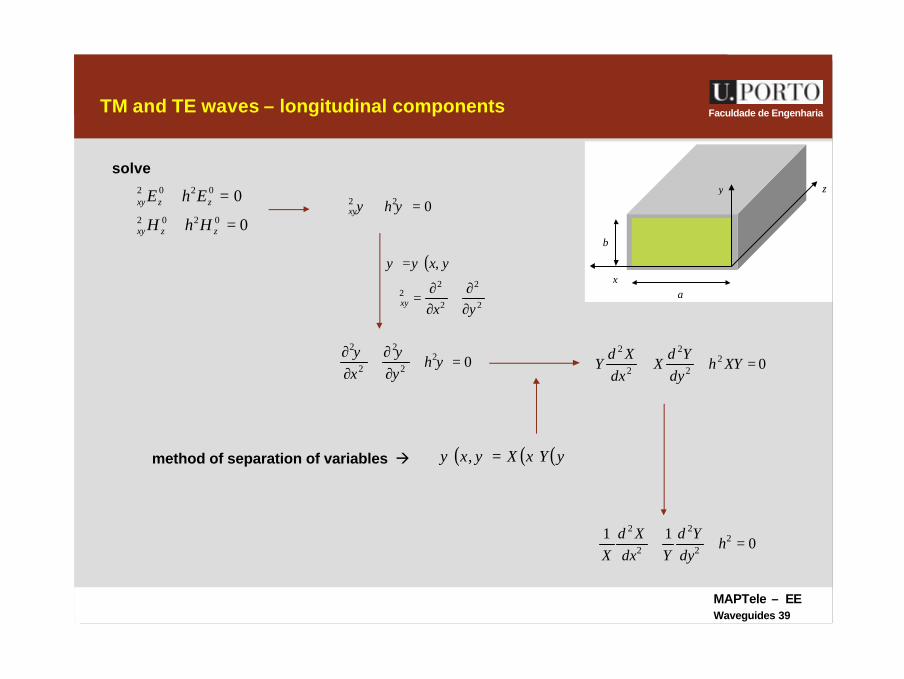
Faculdade de EngenhariaTM and TE waves – longitudinal components
b
y z
x a
0
00202
0202
=+∇
=+∇
zzxy
zzxy
HhH
EhE
solve
022 =+∇ ψψ hxy
( )yx,ψψ =
2
2
2
22
yxxy ∂∂
+∂∂
=∇
022
2
2
2
=+∂∂
+∂∂
ψψψ
hyx
( ) ( ) ( )yYxXyx =,ψmethod of separation of variables à
022
2
2
2
=++ XYhdy
YdX
dxXd
Y
011 2
2
2
2
2
=++ hdy
YdYdx
XdX
MAPTele – EEWaveguides 40
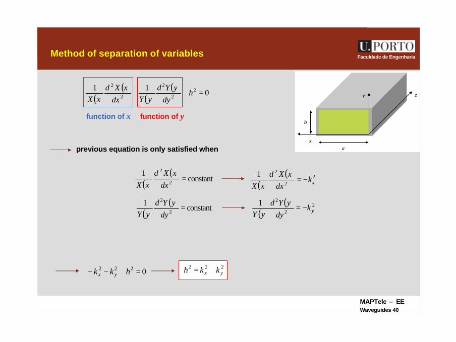
Faculdade de EngenhariaMethod of separation of variables
b
y z
x a
( )( )
( )( )
011 2
2
2
2
2
=++ hdy
yYdyYdx
xXdxX
function of x function of y
previous equation is only satisfied when
( )( )
constant1
2
2
=dx
xXdxX
( )( )
constant1
2
2
=dy
yYdyY
( )( ) 22
21xk
dxxXd
xX−=
( )( ) 22
21yk
dyyYd
yY−=
0222 =+−− hkk yx222yx kkh +=
MAPTele – EEWaveguides 41
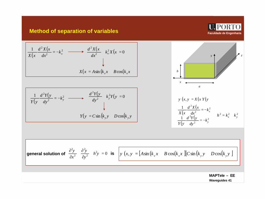
Faculdade de EngenhariaMethod of separation of variables
b
y z
x a
( )( ) 22
21xk
dxxXd
xX−=
( )( ) 22
21yk
dyyYd
yY−=
222yx kkh +=
( )( ) 22
21xk
dxxXd
xX−=
( )( ) 22
21yk
dyyYd
yY−=
( ) ( ) 022
2
=+ xXkdx
xXdx
( ) ( ) 022
2
=+ yYkdy
yYdy
( ) ( ) ( )xkBxkAxX xx cossin +=
( ) ( ) ( )ykDykCyY yy cossin +=
general solution of is
( ) ( ) ( )yYxXyx =,ψ
022
2
2
2
=+∂∂
+∂∂
ψψψ
hyx
( ) ( ) ( )[ ] ( ) ( )[ ]ykDykCxkBxkAyx yyxx cossincossin, ++=ψ
MAPTele – EEWaveguides 42
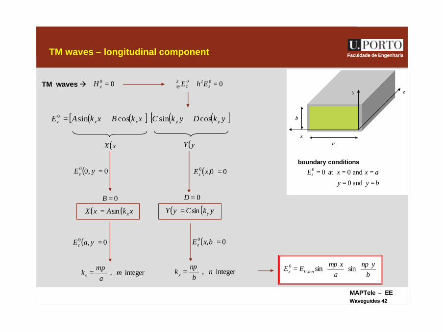
Faculdade de EngenhariaTM waves – longitudinal component
b
y z
x a
TM waves à 00 =zH 00202 =+∇ zzxy EhE
( ) ( )[ ] ( ) ( )[ ]ykDykCxkBxkAE yyxxz cossincossin0 ++=
( )xX ( )yY
boundary conditions
byy
axxEz
=====
and0
and0at00( ) 0,00 =yEz
( ) 0,0 =bxEz( ) 0,0 =yaEz
0=B
( ) ( )xkAxX xsin=
integer, ma
mkx
π= integer, n
bn
kyπ
=
( ) 00,0 =xEz
0=D
( ) ( )ykCyY ysin=
=
byn
axmEE mnz
ππ sinsin,00
MAPTele – EEWaveguides 43
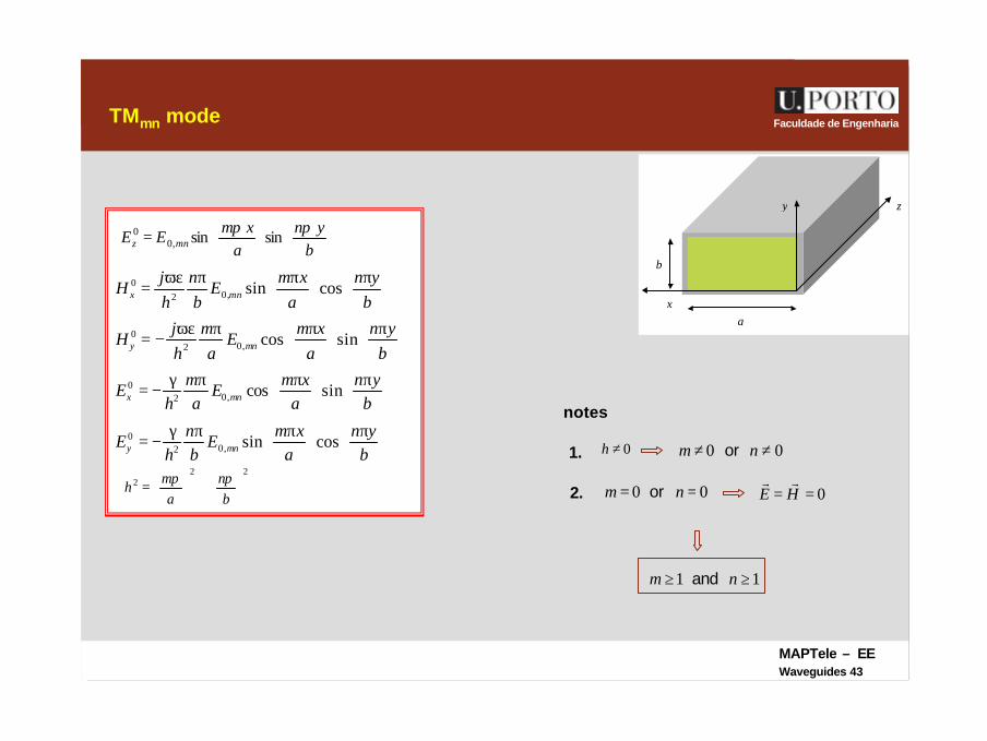
Faculdade de EngenhariaTMmn mode
b
y z
x a
=
byn
axmEE mnz
ππ sinsin,00
00,2
00,2
00,2
00,2
sin cos
cos sin
cos sin
sin cos
x mn
y mn
x mn
y mn
j n m x n yH E
h b a bj m m x n y
H Eh a a b
m m x n yE E
h a a b
n m x n yE E
h b a b
ωε π π π =
ωε π π π = −
γ π π π = −
γ π π π = −
222
+
=
bn
amh ππ
notes
2.
0≠h 00 ≠≠ nm or1.
00 == nm or 0== HErr
11 ≥≥ nm and
MAPTele – EEWaveguides 44
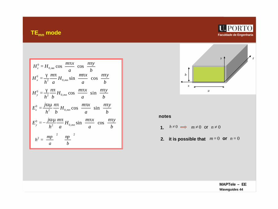
Faculdade de EngenhariaTEmn mode
b
y z
x a
222
+
=
bn
am
hππ
notes
2.
0≠h 00 ≠≠ nm or1.
00 == nm or
00, cos cosz mn
m x n yH H
a bπ π =
0
0,2
00,2
00,2
00,2
sin cos
cos sin
cos sin
sin cos
x mn
y mn
x mn
y mn
m m x n yH H
h a a b
n m x n yH H
h b a b
j n m x n yE H
h b a b
j m m x n yE H
h a a b
γ π π π =
γ π π π = ωµ π π π =
ωµ π π π = −
it is possible that
MAPTele – EEWaveguides 45
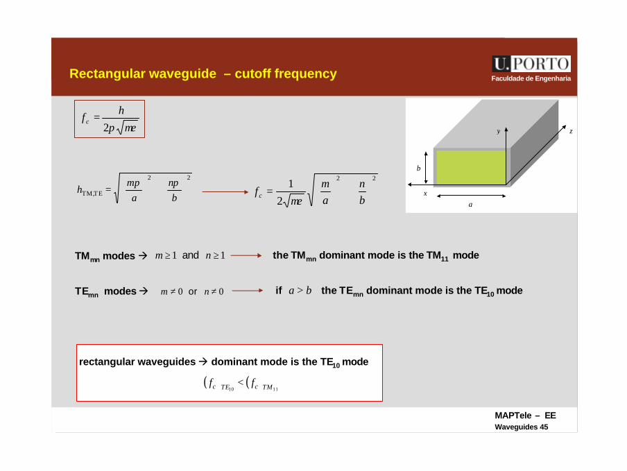
Faculdade de EngenhariaRectangular waveguide – cutoff frequency
µεπ2
hf c =
rectangular waveguides à dominant mode is the TE10 mode
22
TETM,
+
=
bn
am
hππ 22
21
+
=
bn
am
f c µε
b
y z
x a
TMmn modes à 11 ≥≥ nm and the TMmn dominant mode is the TM11 mode
TEmn modes à if the TEmn dominant mode is the TE10 mode00 ≠≠ nm or ba >
( ) ( )1110 TMcTEc ff <

MAPTele – EEWaveguides 46
Faculdade de EngenhariaCircular waveguides
waveguide filled with lossless dielectric ( )µε ,
ideal conducting surface ( )∞=σ
infinite length à propagation along +z
z
φ
a
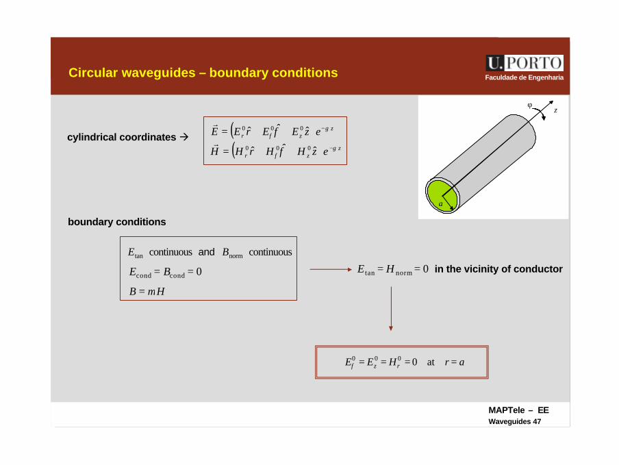
MAPTele – EEWaveguides 47
Faculdade de EngenhariaCircular waveguides – boundary conditions
0condcond == BE
continuoustanE continuousnormBand
boundary conditions
HB µ=
0normtan == HE in the vicinity of conductor
cylindrical coordinates à ( ) zzr ezEErEE γ
φ φ −++= ˆˆˆ 000r
( ) zzr ezHHrHH γ
φ φ −++= ˆˆˆ 000r
z
φ
a
arHEE rz ==== at0000φ
MAPTele – EEWaveguides 48
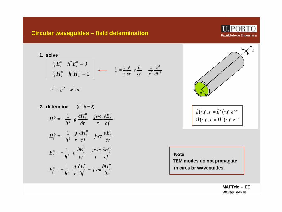
Faculdade de EngenhariaCircular waveguides – field determination
(if )0≠h2. determine
µεωγ 222 +=h
1. solve
( ) ( )( ) ( ) z
z
erHzrH
erEzrEγ
γ
φφ
φφ−
−
=
=
,,,
,,,0
0
rr
rr
0
00202
0202
=+∇
=+∇
zzr
zzr
HhH
EhE
φ
φ
2
2
22 11
φφ ∂∂+
∂∂
∂∂=∇
rrr
rrr
z
φ
a
∂
∂−∂
∂−=
∂
∂+∂
∂−=
∂
∂+∂
∂−=
∂∂−
∂∂−=
rHjE
rhE
Hr
jr
Eh
E
rEjH
rhH
Er
jr
Hh
H
zz
zzr
zz
zzr
00
20
00
20
00
20
00
20
1
1
1
1
ωµφ
γ
φωµγ
ωεφ
γ
φωεγ
φ
φ
NoteTEM modes do not propagatein circular waveguides
MAPTele – EEWaveguides 49
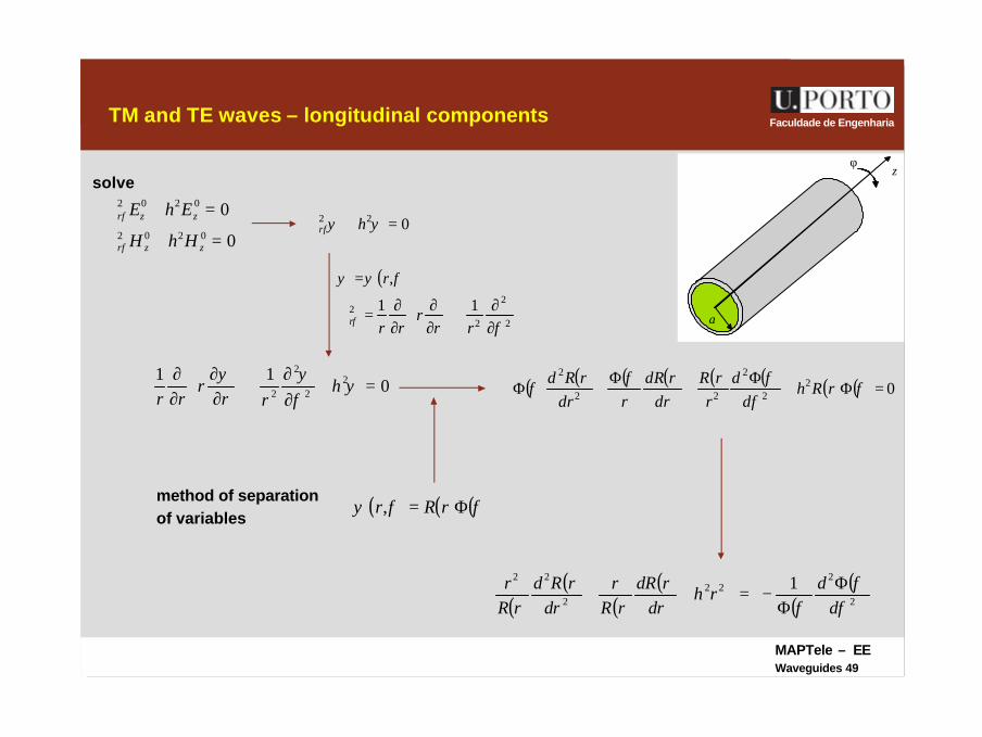
Faculdade de EngenhariaTM and TE waves – longitudinal components
solve
022 =+∇ ψψφ hr
( )φψψ ,r=
method of separation of variables
0
00202
0202
=+∇
=+∇
zzr
zzr
HhH
EhE
φ
φ
2
2
22 11
φφ ∂∂+
∂∂
∂∂=∇
rrr
rrr
z
φ
a
011 2
2
2
2 =+∂∂
+
∂∂
∂∂
ψφψψ
hrr
rrr
( ) ( ) ( )φφψ Φ= rRr,
( )( )
( )( )
( )( )2
222
2
22 1φ
φφ d
drh
drrdR
rRr
drrRd
rRr Φ
Φ−=++
( ) ( ) ( ) ( ) ( ) ( ) ( ) ( ) 022
2
22
2
=Φ+Φ
+Φ
+Φ φφ
φφφ rRh
dd
rrR
drrdR
rdrrRd
MAPTele – EEWaveguides 50
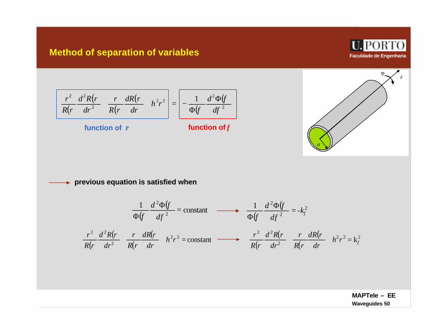
Faculdade de EngenhariaMethod of separation of variables
function of r function of φ
previous equation is satisfied when
( )( )
constant1
2
2
=Φ
Φ φφ
φ dd
( )( )
( )( )
( )( )2
222
2
22 1φ
φφ d
drh
drrdR
rRr
drrRd
rRr Φ
Φ−=++
( )( )
( )( )
constant222
22
=++ rhdr
rdRrR
rdr
rRdrR
r
( )( ) 22
2
-1
φφ
φφ
kd
d=
ΦΦ
( )( )
( )( ) 222
2
22
kφ=++ rhdr
rdRrR
rdr
rRdrR
r
z
φ
a
MAPTele – EEWaveguides 51
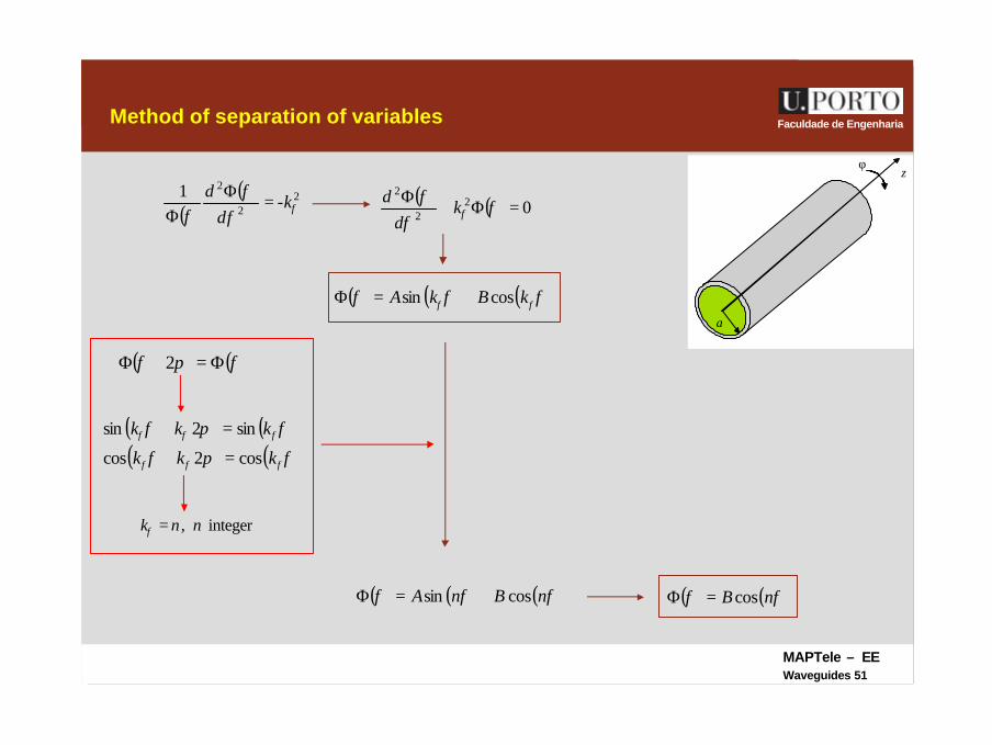
Faculdade de EngenhariaMethod of separation of variables
( )( ) 22
2
-1
φφ
φφ
kd
d=
ΦΦ
( ) ( ) 022
2
=Φ+Φ
φφ
φφk
dd
( ) ( ) ( )φφφ φφ kBkA cossin +=Φ
z
φ
a
( ) ( )φπφ Φ=+Φ 2
( ) ( )( ) ( )φπφ
φπφ
φφφ
φφφ
kkk
kkk
cos2cos
sin2sin
=+
=+
integer, nnk =φ
( ) ( ) ( )φφφ nBnA cossin +=Φ ( ) ( )φφ nB cos=Φ
MAPTele – EEWaveguides 52
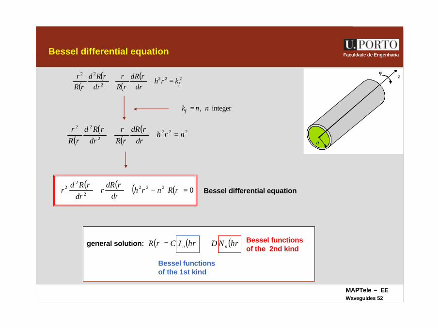
Faculdade de EngenhariaBessel differential equation
z
φ
a
integer, nnk =φ
( )( )
( )( ) 222
2
22
φkrhdr
rdRrR
rdr
rRdrR
r=++
( )( )
( )( ) 222
2
22
nrhdr
rdRrR
rdr
rRdrR
r=++
Bessel differential equation( ) ( ) ( ) ( ) 02222
22 =−++ rRnrh
drrdR
rdr
rRdr
( ) ( ) ( )hrNDhrJCrR nn +=general solution:
Bessel functionsof the 1st kind
Bessel functionsof the 2nd kind
MAPTele – EEWaveguides 53
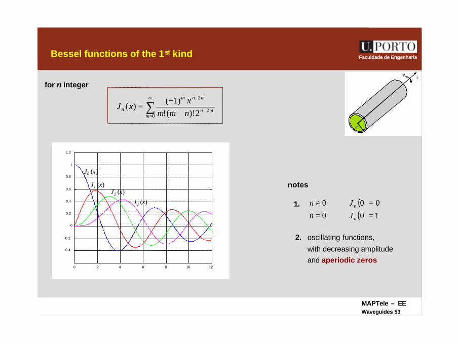
Faculdade de EngenhariaBessel functions of the 1st kind
z
φ
a
for n integer
∑∞
=+
+
+−
=0
2
2
2)!(!)1(
)(m
mn
mnm
n nmmx
xJ
0 2 4 6 8 10 12
-0.4
-0.2
0
0.2
0.4
0.6
0.8
1
1.2
J0 (x)
J1 (x)J2 (x)
J3 (x) ( )( ) 100
000
=⇒=
=⇒≠
n
n
Jn
Jn
notes
2. oscillating functions,
with decreasing amplitudeand aperiodic zeros
1.
MAPTele – EEWaveguides 54
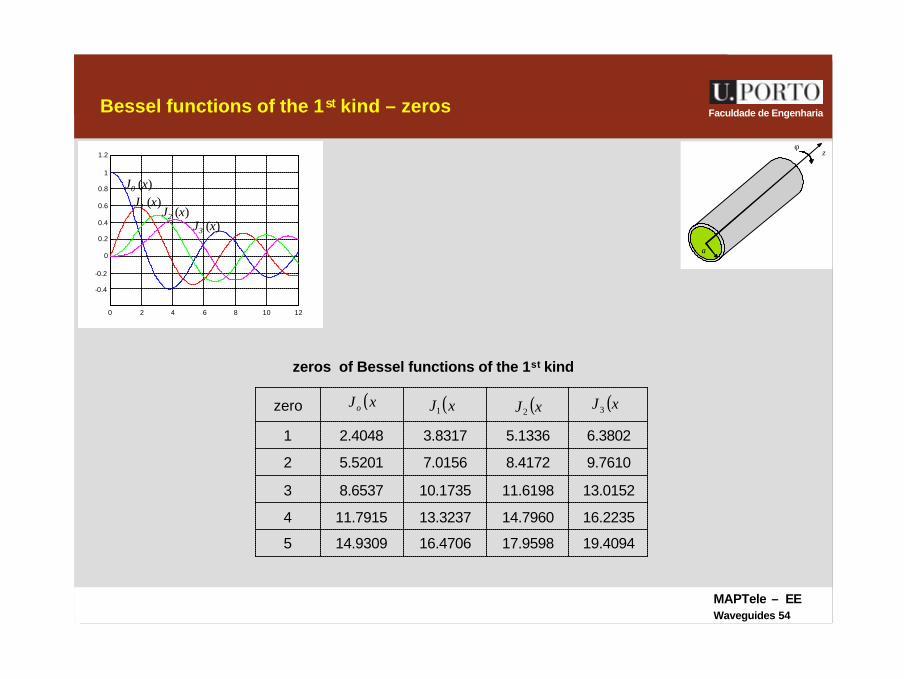
Faculdade de EngenhariaBessel functions of the 1st kind – zeros
z
φ
a
0 2 4 6 8 10 12
-0.4
-0.2
0
0.2
0.4
0.6
0.8
1
1.2
J0 (x)J1 (x)
J2 (x)J3 (x)
( )xJo ( )xJ1 ( )xJ2( )xJ3
19.409417.959816.470614.93095
16.223514.796013.323711.79154
13.015211.619810.17358.65373
9.76108.41727.01565.52012
6.38025.13363.83172.40481
zero
zeros of Bessel functions of the 1st kind
MAPTele – EEWaveguides 55
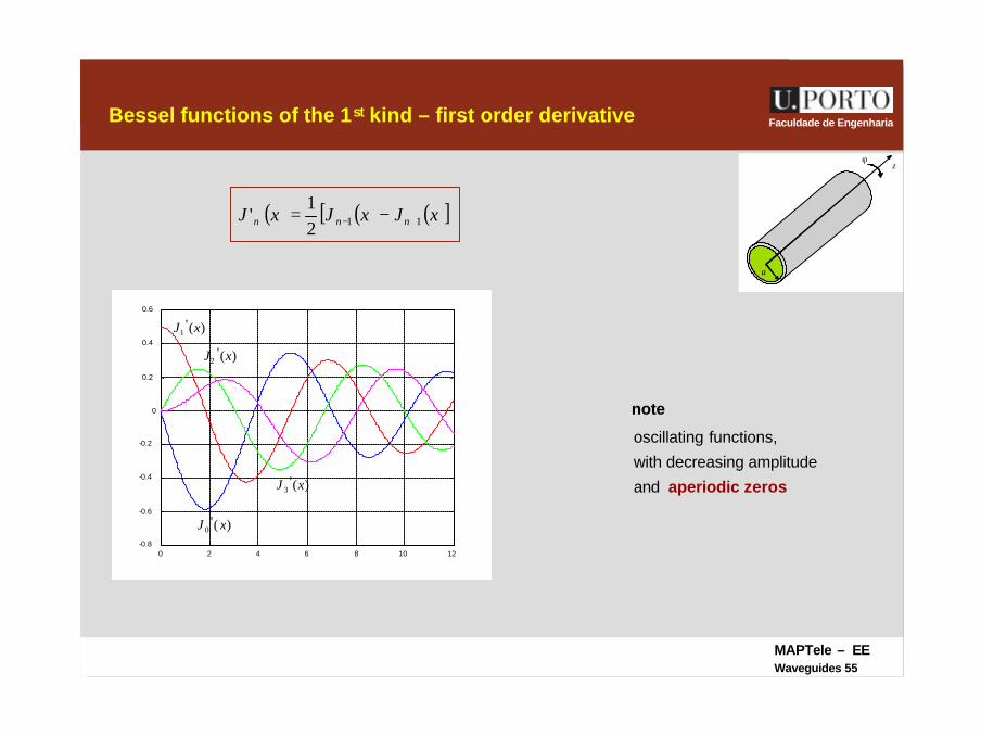
Faculdade de EngenhariaBessel functions of the 1st kind – first order derivative
z
φ
a
note
oscillating functions,
with decreasing amplitude
and aperiodic zeros
( ) ( ) ( )[ ]xJxJxJ nnn 1121
' +− −=
0 2 4 6 8 10 12-0.8
-0.6
-0.4
-0.2
0
0.2
0.4
0.6
)('1 xJ
)('2 xJ
)('3 xJ
)('0 xJ
MAPTele – EEWaveguides 56
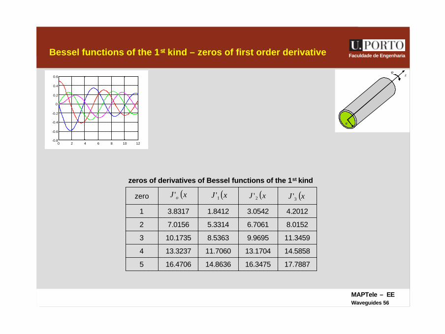
Faculdade de EngenhariaBessel functions of the 1st kind – zeros of first order derivative
z
φ
a
zeros of derivatives of Bessel functions of the 1st kind
0 2 4 6 8 10 12-0.8
-0.6
-0.4
-0.2
0
0.2
0.4
0.6
( )xJ o' ( )xJ 1' ( )xJ 2' ( )xJ 3'
17.788716.347514.863616.47065
14.585813.170411.706013.32374
11.34599.96958.536310.17353
8.01526.70615.33147.01562
4.20123.05421.84123.83171
zero
MAPTele – EEWaveguides 57
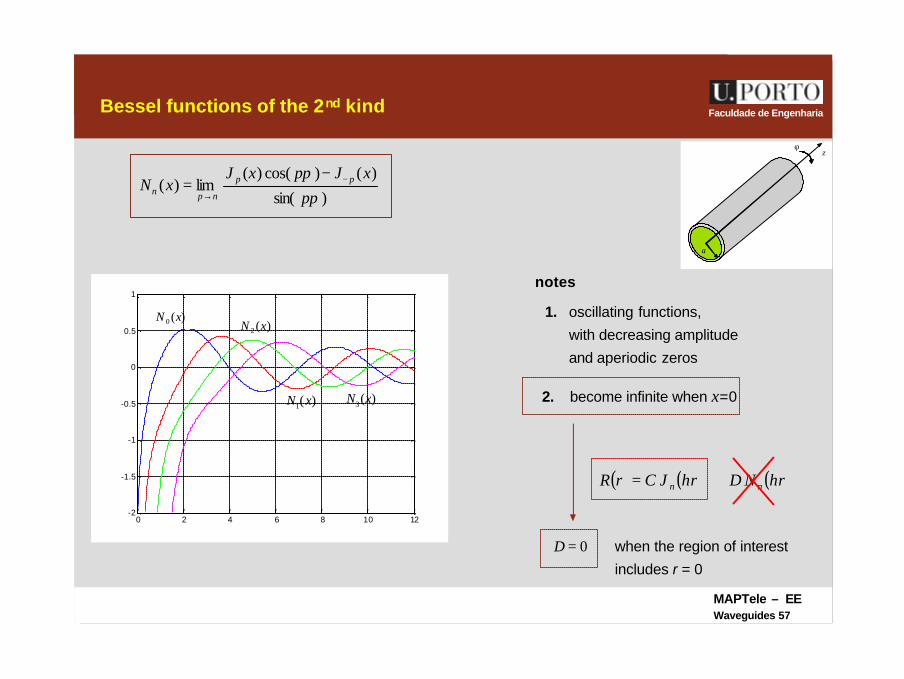
Faculdade de EngenhariaBessel functions of the 2nd kind
z
φ
a
notes
1. oscillating functions,
with decreasing amplitude
and aperiodic zeros
)sin(
)()cos()(lim)(
ππp
xJpxJxN pp
npn−
→
−=
0 2 4 6 8 10 12-2
-1.5
-1
-0.5
0
0.5
1
)(0 xN
)(1 xN
)(2 xN
)(3 xN 2. become infinite when x=0
( ) ( ) ( )hrNDhrJCrR nn +=
0=D when the region of interest
includes r = 0
MAPTele – EEWaveguides 58
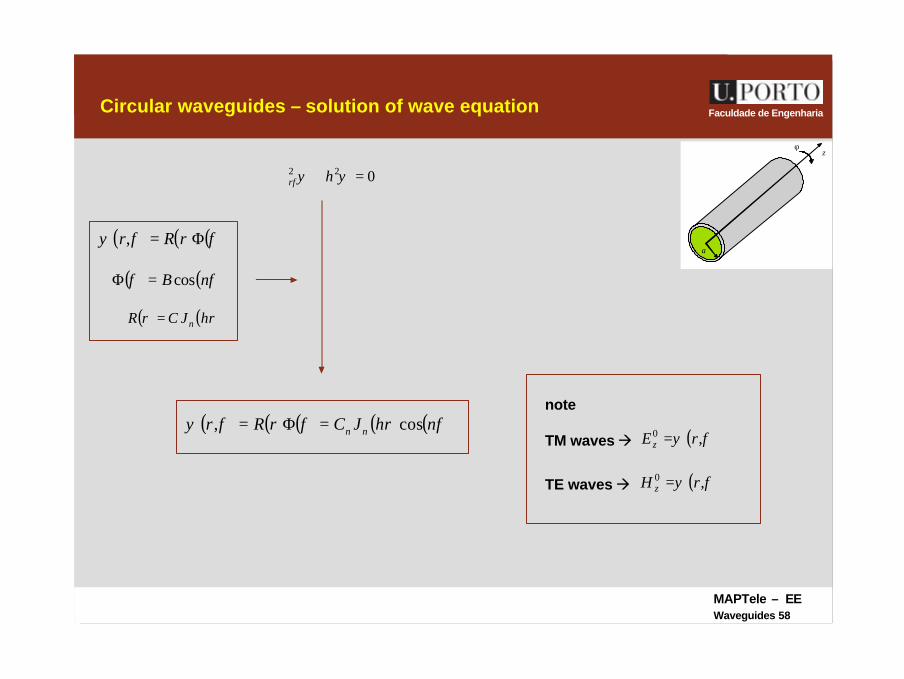
Faculdade de EngenhariaCircular waveguides – solution of wave equation
z
φ
a
note
TM waves à
( ) ( )hrJCrR n=
022 =+∇ ψψφ hr
( ) ( ) ( )φφψ Φ= rRr,
( ) ( )φφ nB cos=Φ
( ) ( ) ( ) ( ) ( )φφφψ nhrJCrRr nn cos, =Φ=( )φψ ,0 rE z =
TE waves à ( )φψ ,0 rH z =
MAPTele – EEWaveguides 59
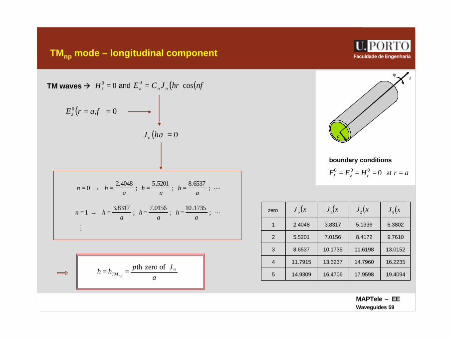
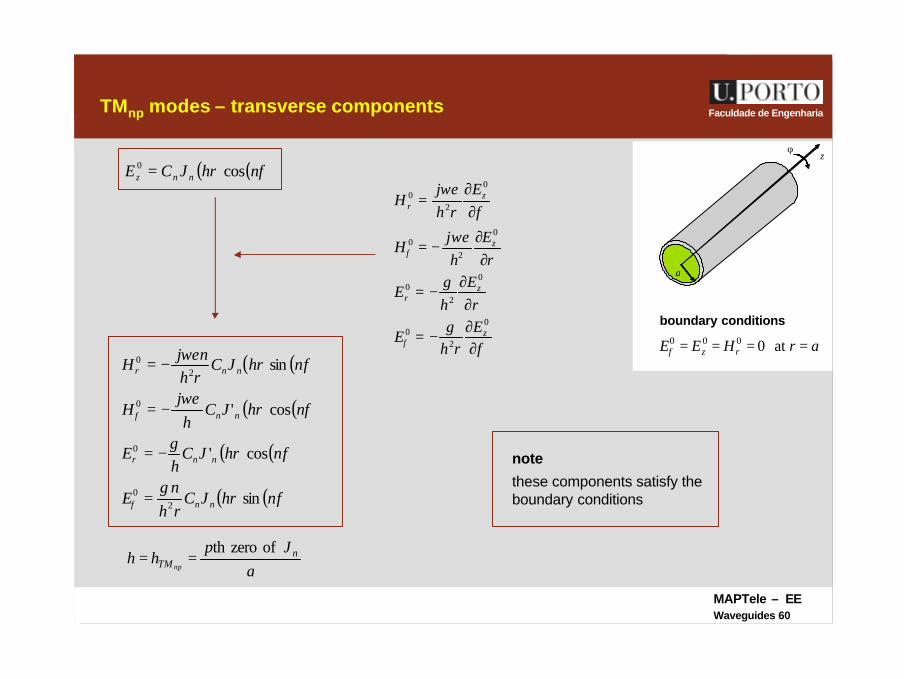
Faculdade de EngenhariaTMnp mode – longitudinal component
TM waves à 00 =zH
boundary conditions
z
φ
a
arHEE rz ==== at0000φ
( ) 0,0 == φarEz
and ( ) ( )φnhrJCE nnz cos0 =
( ) 0=haJ n
( )xJ o ( )xJ1 ( )xJ2 ( )xJ3
19.409417.959816.470614.93095
16.223514.796013.323711.79154
13.015211.619810.17358.65373
9.76108.41727.01565.52012
6.38025.13363.83172.40481
zero
L;6537.8
;5201.5
;4048.2
0a
ha
ha
hn ===→=
L;1735.10
;0156.7
;8317.3
1a
ha
ha
hn ===→=
M
aJp
hh nTMnp
ofzeroth==
MAPTele – EEWaveguides 60
Faculdade de EngenhariaTMnp modes – transverse components
boundary conditions
z
φ
a
arHEE rz ==== at0000φ
( ) ( )φnhrJCE nnz cos0 =
φγ
γ
ωε
φωε
φ
φ
∂∂
−=
∂∂
−=
∂∂
−=
∂∂
=
0
20
0
20
0
20
0
20
z
zr
z
zr
Erh
E
rE
hE
rE
hj
H
Erh
jH
( ) ( )
( ) ( )
( ) ( )
( ) ( )φγ
φγ
φωε
φωε
φ
φ
nhrJCrhn
E
nhrJCh
E
nhrJCh
jH
nhrJCrhnj
H
nn
nnr
nn
nnr
sin
cos'
cos'
sin
20
0
0
20
=
−=
−=
−=
these components satisfy theboundary conditions
note
aJp
hh nTM np
ofzeroth==
MAPTele – EEWaveguides 61
Faculdade de EngenhariaTMnp modes – cutoff frequency
z
φ
a
aJp
h nTM np
ofzeroth=
( )µεπ2np
np
TMTMc
hf =
µεπ a
Jp n
2
ofzeroth=
( )xJ o ( )xJ1 ( )xJ2 ( )xJ3
19.409417.959816.470614.93095
16.223514.796013.323711.79154
13.015211.619810.17358.65373
9.76108.41727.01565.52012
6.38025.13363.83172.40481
zero
lowest zero of à 2.4048 (n=0, p=1)nJ
( )µεπ a
f TMc2
4048.201
=
dominant TM mode à TM01
MAPTele – EEWaveguides 62
Faculdade de EngenhariaTEnp modes
TE waves à 00 =zE
boundary conditions
z
φ
a
arHEE rz ==== at0000φ
e ( ) ( )φnhrJCH nnz cos0 =
rH
hj
E
Hrh
jE
Hrh
H
rH
hH
z
zr
z
zr
∂∂
=
∂∂
−=
∂∂
−=
∂∂
−=
0
20
0
20
0
20
0
20
ωµ
φωµ
φγ
γ
φ
φ
( ) ( )
( ) ( )
( ) ( )
( ) ( )φωµ
φωµ
φγ
φγ
φ
φ
nhrJCh
jE
nhrJCrhnj
E
nhrJCrhn
H
nhrJCh
H
nn
nnr
nn
nnr
cos'
sin
sin
cos'
0
20
20
0
=
=
=
−=
( ) 0' =haJ n
aJp
hh nTEnp
'ofzeroth==
MAPTele – EEWaveguides 63
Faculdade de EngenhariaTEnp modes – cutoff frequency
z
φ
a
( )µεπ2np
np
TETEc
hf =
µεπ a
Jp n
2
ofzeroth /
=
lowest zero of à 1.8412 (n=1, p=1)/nJ
dominant TE mode à TE11
aJp
hh nTEnp
'ofzeroth==
( )xJ o' ( )xJ 1' ( )xJ 2' ( )xJ 3'
17.788716.347514.863616.47065
14.585813.170411.706013.32374
11.34599.96958.536310.17353
8.01526.70615.33147.01562
4.20123.05421.84123.83171
zero
( )µεπ a
f TEc2
8412.111
=
( ) ( )0111 TMcTEc ff < dominant mode in circular
waveguides is TE11
MAPTele – EEWaveguides 64
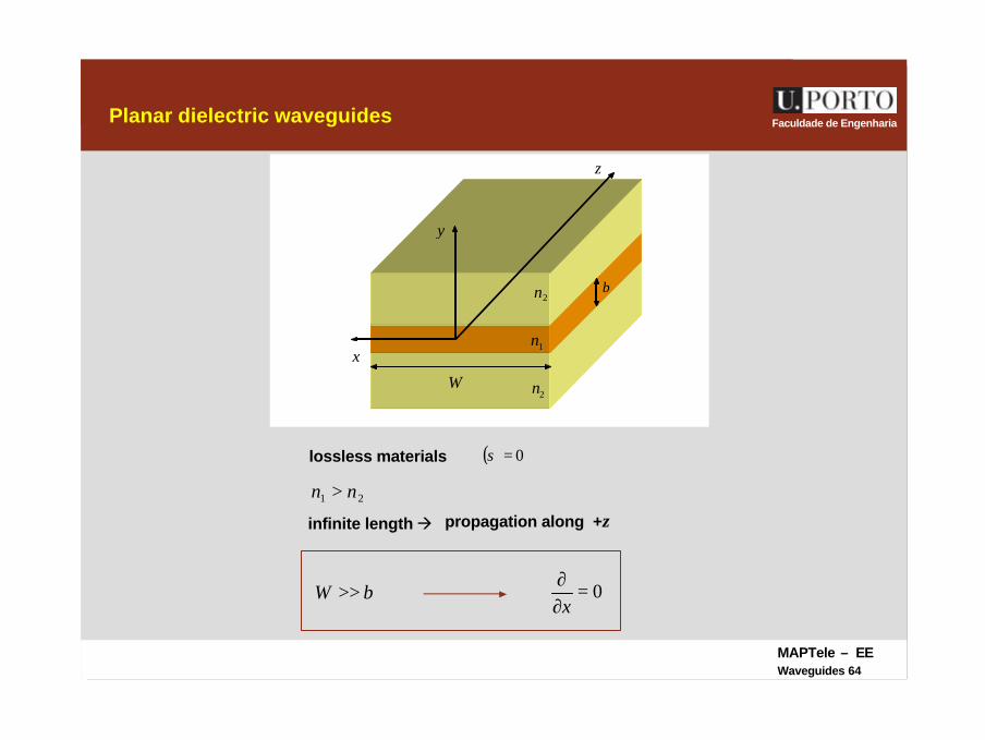
Faculdade de EngenhariaPlanar dielectric waveguides
lossless materials ( )0=σ
infinite length à propagation along +z
W
z
y
x
b
2n
1n
2n
21 nn >
bW >> 0=∂∂x
MAPTele – EEWaveguides 65
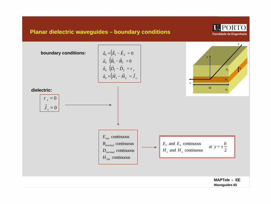
Faculdade de EngenhariaPlanar dielectric waveguides – boundary conditions
boundary conditions:
W
z
y
x
b
2n
1n
2n
0=sρ
0=sJr
continuous
continuous
continuous
continuous
tan
tan
H
D
B
E
normal
normal
( )( )( )( ) sn
sn
n
n
JHHa
DDa
BBa
EEa
rrr
rr
rr
rr
=−×
=−⋅
=−⋅
=−×
21
21
21
21
ˆ
ˆ
0ˆ
0ˆ
ρ
dielectric:
continuousandcontinuousand
xz
xz
HHEE
2at
by ±=

MAPTele – EEWaveguides 66
Faculdade de EngenhariaPlanar dielectric waveguide – field determination
(if )0≠h2. determine
µεωγ 222 +=h
1. solve
( ) ( )( ) ( ) z
z
eyxHzyxH
eyxEzyxEγ
γ
−
−
=
=
,,,
,,,0
0
rr
rr
0
0
022
02
022
02
=+
=+
zz
zz
Hhdy
Hd
Ehdy
Ed
W
z
y
x
b
2n
1n
2n
0=∂∂x
dydE
hE
dydH
hj
E
dydH
hH
dydE
hj
H
zy
zx
zy
zx
0
20
0
20
0
20
0
20
γ
ωµ
γ
ωε
−=
−=
−=
=
+
+=
2medium,
1medium,
2
22
2
12
2
nc
nch
ωγ
ωγ
21h
22h
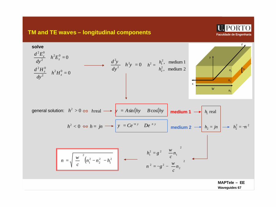
MAPTele – EEWaveguides 67
Faculdade de EngenhariaTM and TE waves – longitudinal components
0
0
022
02
022
02
=+
=+
zz
zz
Hhdy
Hd
Ehdy
Ed
W
z
y
x
b
2n
1n
2n
=2medium,
1medium,22
212
h
hh
solve
022
2
=+ ψψ hdyd
general solution: 02 >h
νjh =
realh ( ) ( )hyBhyA cossin +=ψ
02 <h yy DeCe ννψ +− +=
medium 1
medium 2
real1h
νjh =222
2 ν−=h
−−=
+=
2
222
2
122
1
nc
nc
h
ωγν
ωγ
( ) 21
22
21
2
hnnc
−−
= ων
MAPTele – EEWaveguides 68
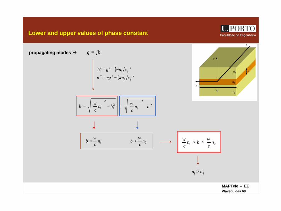
Faculdade de EngenhariaLower and upper values of phase constant
W
z
y
x
b
2n
1n
2n
propagating modes à βγ j=
( )( )2
1222
211
221
cn
cnh
ωγν
ωγ
−−=
+=
21
2
1 hnc
−
=
ωβ 2
2
2 νω
+
= n
c
21 nc
nc
ωβ
ω>>1n
cω
β < 2ncω
β >
21 nn >
MAPTele – EEWaveguides 69
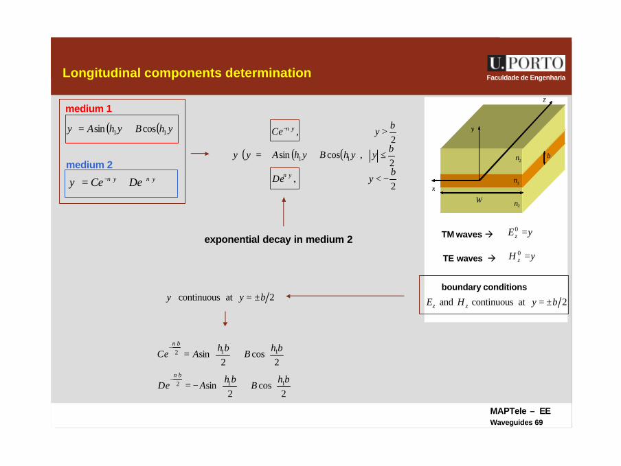
Faculdade de EngenhariaLongitudinal components determination
W
z
y
x
b
2n
1n
2n
( ) ( )yhByhA 11 cossin +=ψ
yy DeCe ννψ +− +=
medium 1
medium 2
TM waves à ψ=0zE
TE waves à ψ=0zH
boundary conditions
2at continuousand byHE zz ±=
( ) ( ) ( )
−<
≤+
>
=
−
2,
2,cossin
2,
11
byDe
byyhByhA
byCe
y
y
y
ν
ν
ψ
exponential decay in medium 2
2at continuous by ±=ψ
+
−=
+
=
−
−
2cos
2sin
2cos
2sin
112
112
bhB
bhADe
bhB
bhACe
b
b
ν
ν
MAPTele – EEWaveguides 70
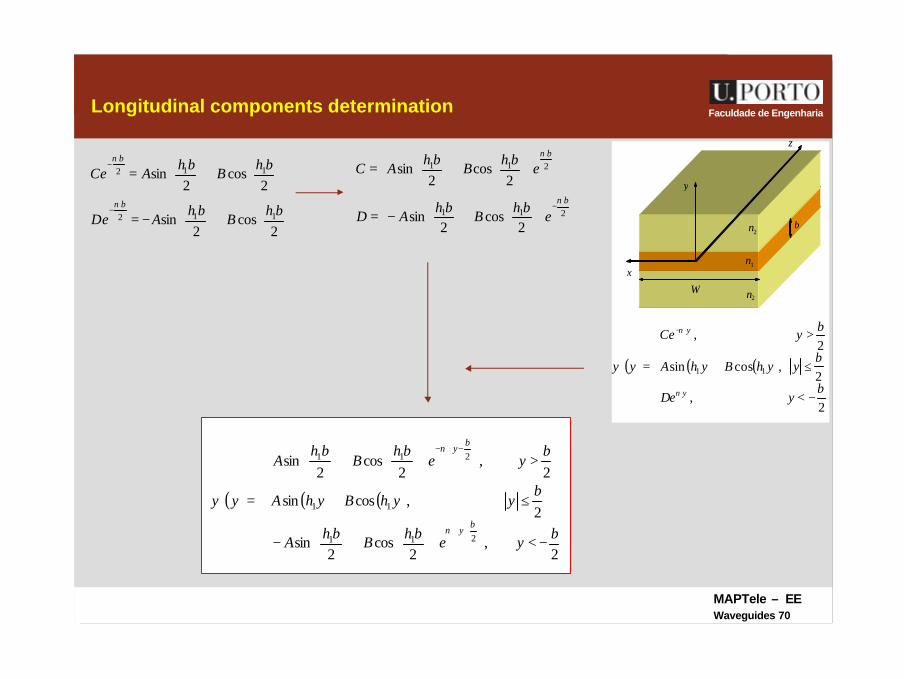
Faculdade de EngenhariaLongitudinal components determination
W
z
y
x
b
2n
1n
2n
+
−=
+
=
−
−
2cos
2sin
2cos
2sin
112
112
bhB
bhADe
bhB
bhACe
b
b
ν
ν
211
211
2cos
2sin
2cos
2sin
b
b
ebh
Bbh
AD
ebh
Bbh
AC
ν
ν
−
+
−=
+
=
( ) ( ) ( )
−<
+
−
≤+
>
+
=
+
−−
2,
2cos
2sin
2,cossin
2,
2cos
2sin
211
11
211
byebhBbhA
byyhByhA
bye
bhB
bhA
yb
y
by
ν
ν
ψ
( ) ( ) ( )
−<
≤+
>
=
−
2,
2,cossin
2,
11
byDe
byyhByhA
byCe
y
y
y
ν
ν
ψ
MAPTele – EEWaveguides 71
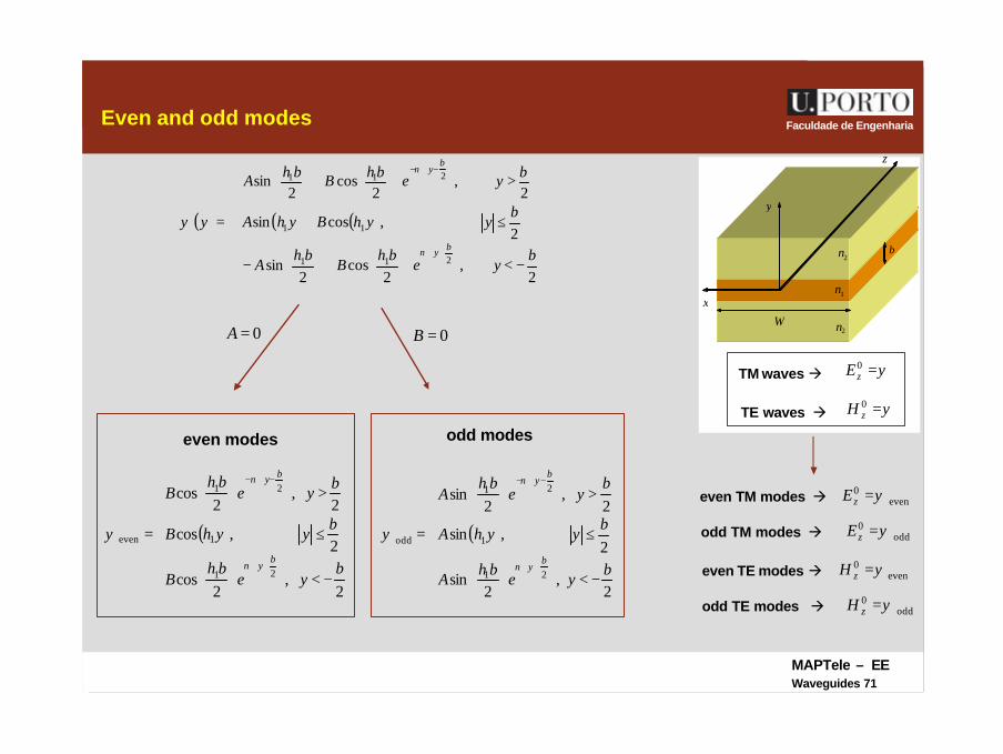
Faculdade de EngenhariaEven and odd modes
W
z
y
x
b
2n
1n
2n
( ) ( ) ( )
−<
+
−
≤+
>
+
=
+
−−
2,
2cos
2sin
2,cossin
2,
2cos
2sin
211
11
211
bye
bhB
bhA
byyhByhA
byebhBbhA
yby
by
ν
ν
ψ
TM waves à ψ=0zE
TE waves à ψ=0zH
even modes
( )
−<
≤
>
=
+
−−
2,
2cos
2,cos
2,
2cos
21
1
21
even
bye
bhB
byyhB
bye
bhB
by
by
ν
ν
ψ
odd modes
( )
−<
≤
>
=
+
−−
2,
2sin
2,sin
2,
2sin
21
1
21
odd
bye
bhA
byyhA
bye
bhA
by
by
ν
ν
ψ
0=A 0=B
odd TM modes à odd0 ψ=zE
even TM modes à even0 ψ=zE
odd TE modes à odd0 ψ=zH
even TE modes à even0 ψ=zH
MAPTele – EEWaveguides 72
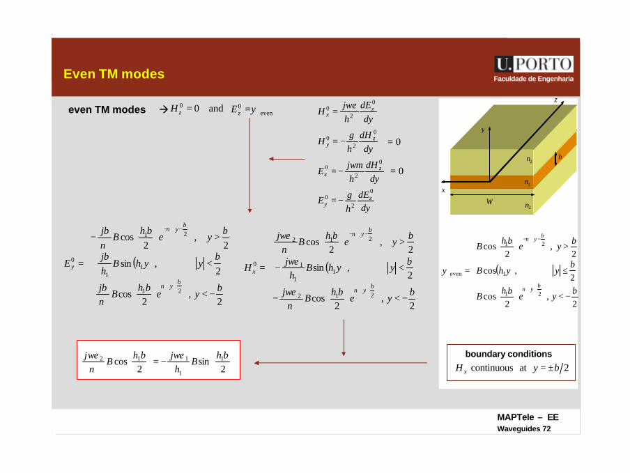
Faculdade de EngenhariaEven TM modes
W
z
y
x
b
2n
1n
2n
( )
−<
≤
>
=
+
−−
2,
2cos
2,cos
2,
2cos
21
1
21
even
byebhB
byyhB
byebhB
by
by
ν
ν
ψ
even TM modes à even0 ψ=zEand00 =zH
dydE
hE
dydH
hj
E
dydH
hH
dydE
hj
H
zy
zx
zy
zx
0
20
0
20
0
20
0
20
γ
ωµ
γ
ωε
−=
−=
−=
=
0=
0=
( )
−<
−
<−
>
=
+
−−
2,
2cos
2,sin
2,
2cos
212
11
1
212
0
bye
bhB
j
byyhB
hj
bye
bhB
j
H
by
by
x
ν
ν
νωε
ωενωε
( )
−<
<
>
−
=
+
−−
2,
2cos
2,sin
2,
2cos
21
11
21
0
bye
bhB
j
byyhB
hj
bye
bhB
j
E
by
by
y
ν
ν
νβ
βνβ
boundary conditions
2at continuous byH x ±=
−=
2sin
2cos 1
1
112 bhB
hjbh
Bj ωενωε
MAPTele – EEWaveguides 73
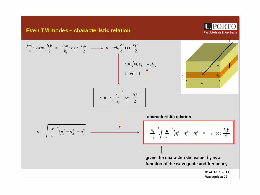
Faculdade de EngenhariaEven TM modes – characteristic relation
W
z
y
x
b
2n
1n
2n
−=
2sin
2cos 1
1
112 bhB
hjbh
Bj ωενωε
−=2
cot 1
1
21
bhh
εε
ν
rrn εµ=
1if =rµ
rε=
−=
2cot 1
2
1
21
bhnn
hν
( ) 21
22
21
2
hnnc
−−
= ων ( )
−=−−
2
cot 11
21
22
21
22
2
1 bhhhnn
cnn ω
characteristic relation
gives the characteristic value h1 as afunction of the waveguide and frequency
MAPTele – EEWaveguides 74
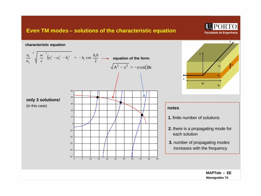
Faculdade de EngenhariaEven TM modes – solutions of the characteristic equation
W
z
y
x
b
2n
1n
2n
( )
−=−−
2
cot 11
21
22
21
22
2
1 bhhhnn
cnn ω
characteristic equation
( )BxxxA cot22 −=−
0 5 10 15 20 25 30 35 40 45 50-50
-40
-30
-20
-10
0
10
20
30
40
50
equation of the form:
only 3 solutions!(in this case) notes
2. there is a propagating mode foreach solution
1. finite number of solutions
3. number of propagating modesincreases with the frequency
MAPTele – EEWaveguides 75
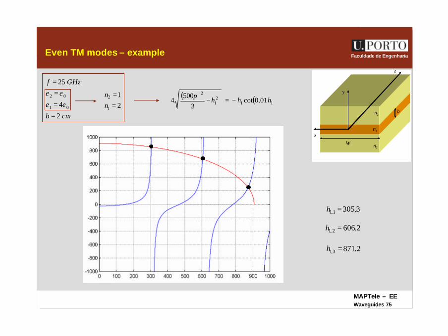
Faculdade de EngenhariaEven TM modes – example
W
z
y
x
b
2n
1n
2n cmb
GHzf
2
4
25
01
02
====
εεεε
21
1
2
==
nn
3.3051,1 =h
2.8713,1 =h
2.6062,1 =h
( ) ( )112
1
2
01.0cot3
5004 hhh −=−
π
MAPTele – EEWaveguides 76
Faculdade de Engenharia
-0.02 -0.015 -0.01 -0.005 0 0.005 0.01 0.015 0.02-1
-0.8
-0.6
-0.4
-0.2
0
0.2
0.4
0.6
0.8
1
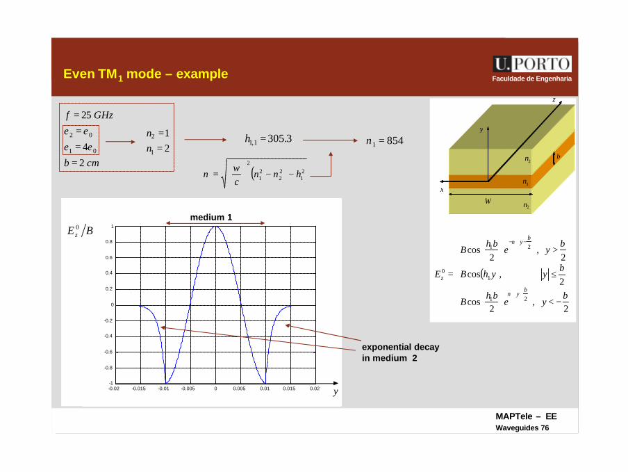
Even TM1 mode – example
W
z
y
x
b
2n
1n
2n cmb
GHzf
2
4
25
01
02
====
εεεε
21
1
2
==
nn 3.3051,1 =h 8541 =ν
( ) 21
22
21
2
hnnc
−−
=
ων
BE z0
( )
−<
≤
>
=
+
−−
2,
2cos
2,cos
2,
2cos
21
1
21
0
bye
bhB
byyhB
bye
bhB
Eb
y
by
z
ν
ν
medium 1
exponential decayin medium 2
y
MAPTele – EEWaveguides 77
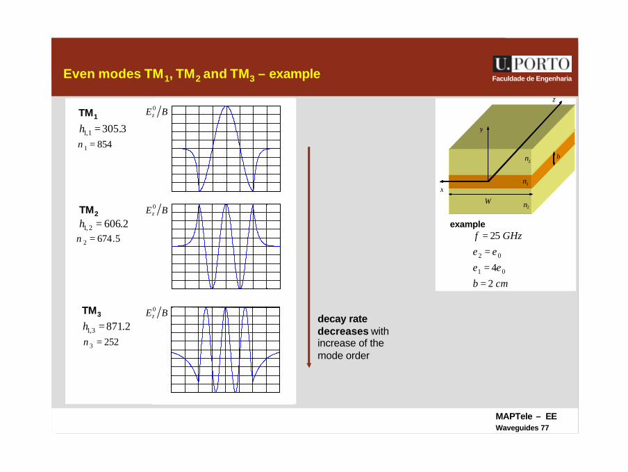
Faculdade de EngenhariaEven modes TM1, TM2 and TM3 – example
W
z
y
x
b
2n
1n
2n
cmb
GHzf
2
4
25
01
02
====
εεεε
2.8713,1 =h
2.6062,1 =h example
8541 =ν
BEz0
BEz0
BEz0
TM1
TM2
TM3
3.3051,1 =h
2523 =ν
5.6742 =ν
decay ratedecreases withincrease of themode order
MAPTele – EEWaveguides 78
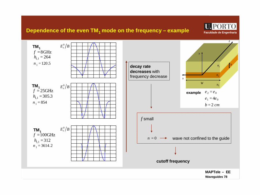
Faculdade de EngenhariaDependence of the even TM1 mode on the frequency – example
W
z
y
x
b
2n
1n
2n
cmb 24 01
02
===
εεεε
3121,1 =h
3.3051,1 =hexample
5.1201 =ν
BEz0TM1
2641,1 =h
2.36141 =ν
8541 =ν
cutoff frequency
TM1
TM1
GHz8=f
GHz25=f
GHz100=f
BEz0
BEz0
decay ratedecreases with frequency decrease
0=ν wave not confined to the guide
f small
MAPTele – EEWaveguides 79
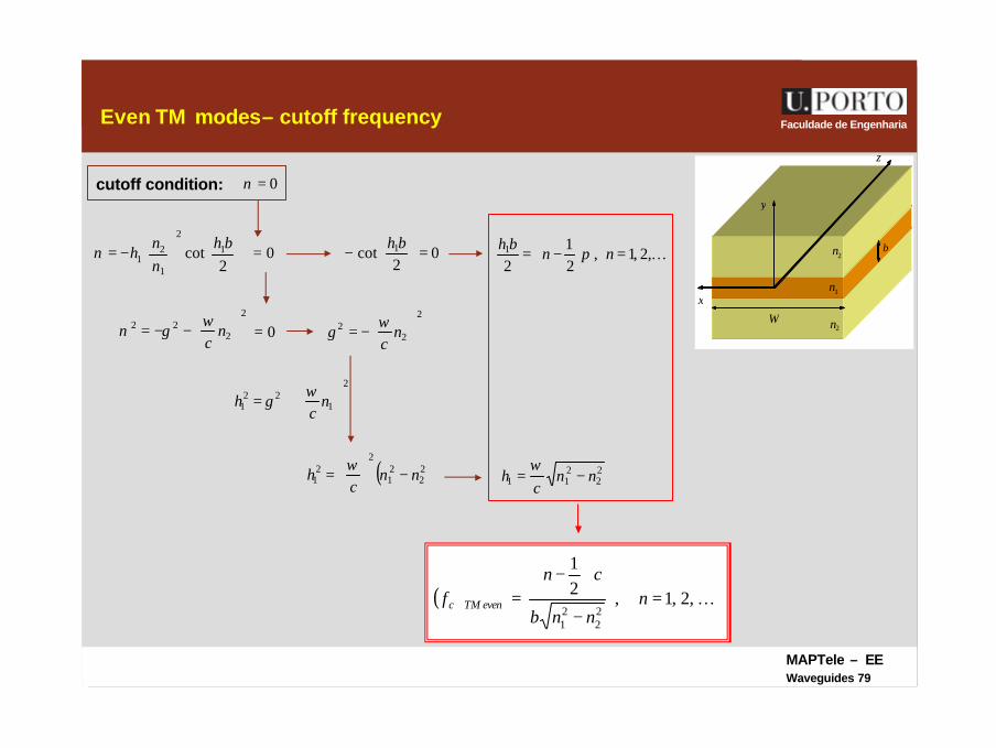
Faculdade de EngenhariaEven TM modes– cutoff frequency
W
z
y
x
b
2n
1n
2n
cutoff condition: 0=ν
2
222
−−= n
cω
γν 0=2
22
−= n
cω
γ
( )22
21
22
1 nnc
h −
=
ω
2
122
1
+= n
ch
ωγ
22
211 nn
ch −=
ω
−=
2cot 1
2
1
21
bhnn
hν 02
cot 1 =
−
bh0= K,2,1,
21
21 =
−= nn
bhπ
( ) K,2,1,21
22
21
=−
−
= nnnb
cnf evenTMc
MAPTele – EEWaveguides 80
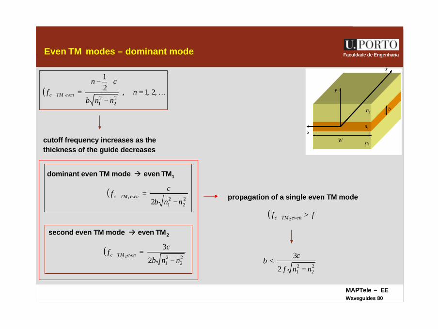
Faculdade de EngenhariaEven TM modes – dominant mode
W
z
y
x
b
2n
1n
2n
( ) K,2,1,21
22
21
=−
−
= nnnb
cnf evenTMc
cutoff frequency increases as thethickness of the guide decreases
dominant even TM mode à even TM1
( )22
212
1nnb
cf evenTMc
−=
second even TM mode à even TM2
( )22
212
32
nnb
cf evenTMc
−=
propagation of a single even TM mode
( ) ff evenTMc >2
22
212
3
nnf
cb
−<
MAPTele – EEWaveguides 81
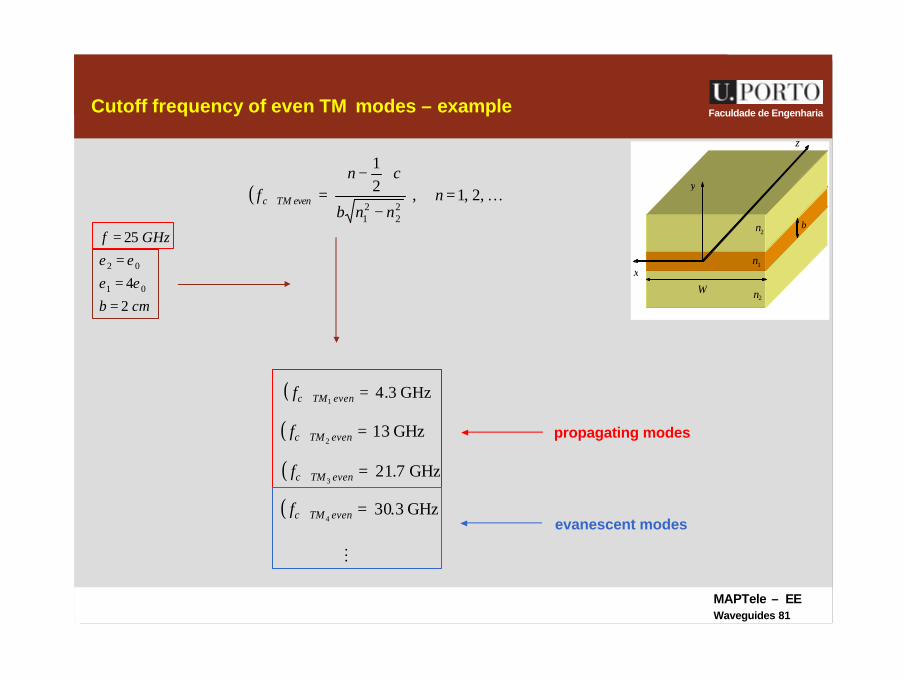
Faculdade de EngenhariaCutoff frequency of even TM modes – example
W
z
y
x
b
2n
1n
2n
( ) K,2,1,21
22
21
=−
−
= nnnb
cnf evenTMc
cmb
GHzf
2
4
25
01
02
====
εεεε
( ) GHz3.41
=evenTMcf
( ) GHz7.213
=evenTMcf
( ) GHz132
=evenTMcf
M
( ) GHz3.304
=evenTMcf
propagating modes
evanescent modes
MAPTele – EEWaveguides 82
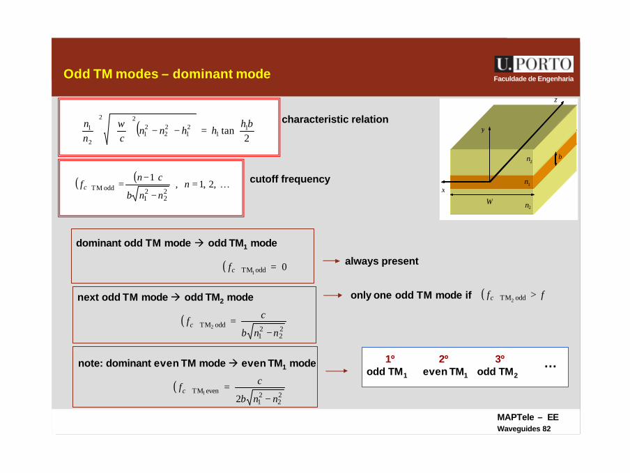
Faculdade de EngenhariaOdd TM modes – dominant mode
W
z
y
x
b
2n
1n
2n
dominant odd TM mode à odd TM1 mode
( ) 0oddTM1=cf
next odd TM modeà odd TM2 mode
( )22
21
oddTM2nnb
cfc
−=
only one odd TM mode if ( ) ffc >oddTM2
( ) ( )K,2,1,
122
21
oddTM =−
−= n
nnb
cnfc
always present
note: dominant even TM modeà even TM1 mode
( )22
21
evenTM2
1nnb
cfc
−=
odd TM1 even TM1 odd TM2
1º 2º 3º …
( )
=−−
2
tan 11
21
22
21
22
2
1 bhhhnn
cnn ω characteristic relation
cutoff frequency
MAPTele – EEWaveguides 83
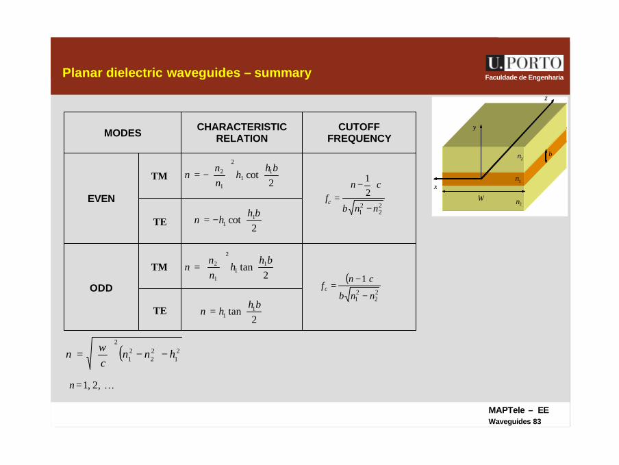
Faculdade de EngenhariaPlanar dielectric waveguides – summary
W
z
y
x
b
2n
1n
2n
−=
2cot 1
1
2
1
2 bhh
nn
ν
22
21
21
nnb
cnfc
−
−
=
−=
2cot 1
1
bhhν
=
2tan 1
1
2
1
2 bhh
nn
ν( )
22
21
1
nnb
cnfc
−
−=
=
2tan 1
1
bhhνTE
TM
ODD
TE
TM
EVEN
CUTOFF FREQUENCY
CHARACTERISTIC RELATIONMODES
( ) 21
22
21
2
hnnc
−−
= ων
K,2,1=n
MAPTele – EEWaveguides 84
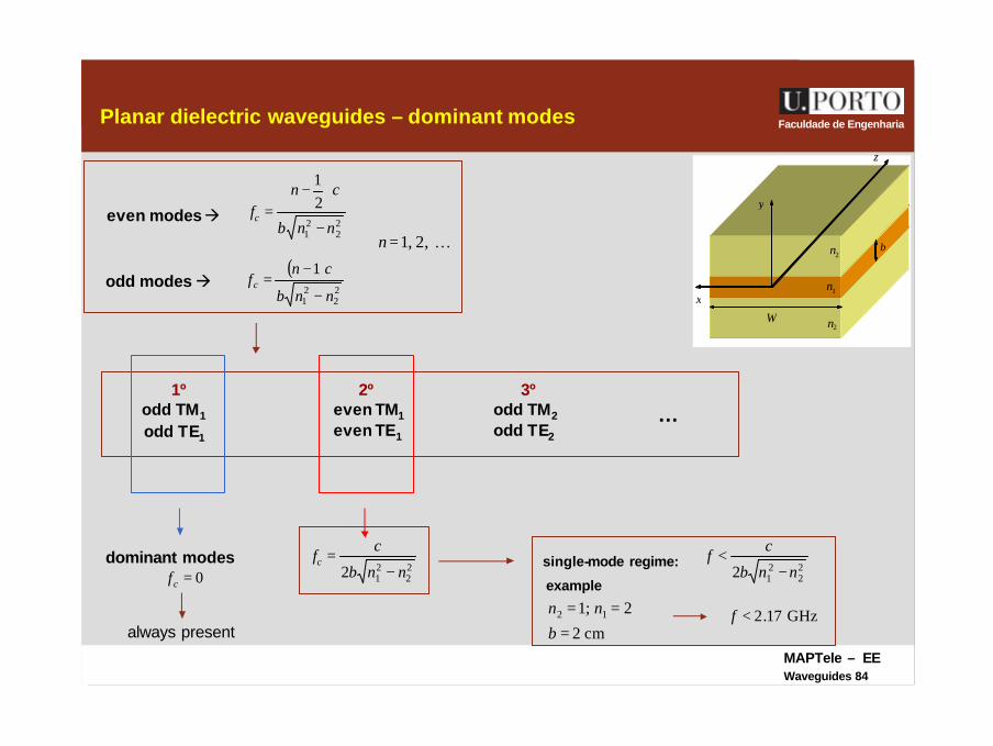
Faculdade de EngenhariaPlanar dielectric waveguides – dominant modes
W
z
y
x
b
2n
1n
2n
odd TM1 even TM1 odd TM2
1º 2º 3º
…
22
21
21
nnb
cnfc
−
−
=
( )22
21
1
nnb
cnfc
−
−=
K,2,1=n
even modesà
odd modesà
odd TE1 even TE1 odd TE2
dominant modes0=cf
always present
22
212 nnb
cfc
−= single-mode regime: 2
2212 nnb
cf
−<
example
cm2
2;1 12
=
==
b
nn GHz17.2<f
MAPTele – EEWaveguides 85
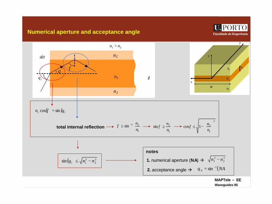
Faculdade de EngenhariaNumerical aperture and acceptance angle
W
z
y
x
b
2n
1n
2n
n1
n2
n2
iθ θ φ
z
air
21 nn >
( ) ( )in θφ sincos1 =
≥ −
1
21sinnn
φtotal internal reflection1
2sinnn
≥φ2
1
21cos
−≤
nn
φ
( ) 22
21sin nni −≤θ
notes
1. numerical aperture (NA) à
2. acceptance angle à
22
21 nn −
( )NAA1sin −=θ
MAPTele – EEWaveguides 86
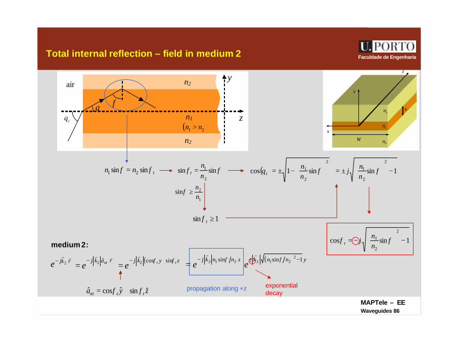
Faculdade de EngenhariaTotal internal reflection – field in medium 2
W
z
y
x
b
2n
1n
2n
n1
n2
n2
iθ θ φ
z
air y
( )21 nn >
1
2sinnn
≥φ
tnn φφ sinsin 21 = φφ sinsin2
1
nn
t =
1sin ≥tφ
( )2
2
1 sin1cos
−±= φθ
nn
t 1sin2
2
1 −
±= φ
nn
j
medium 2:
rkjerr
⋅− 2 rakj nterr
⋅−=
ˆ2
zya ttnt ˆsinˆcosˆ φφ +=
( )zykj tteφφ sincos2 +−
=r ( ) ynnkznnkj
ee1sinsin 2
212212 −±−=
φφrr
propagation along +z exponentialdecay
1sincos2
2
1 −
−= φφ
nn
jt
MAPTele – EEWaveguides 87
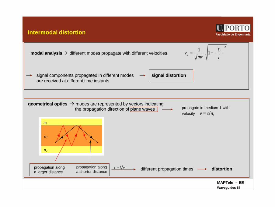
Faculdade de EngenhariaIntermodal distortion
n1
n2
n2
−=
2
11
ff
v cg
εµmodal analysis à different modes propagate with different velocities
propagate in medium 1 withvelocity 1ncv =
geometrical optics à modes are represented by vectors indicatingthe propagation direction of plane waves
propagation alonga shorter distance
propagation alonga larger distance
different propagation timesvlt =
signal components propagated in different modesare received at different time instants
signal distortion
distortion
MAPTele – EEWaveguides 88
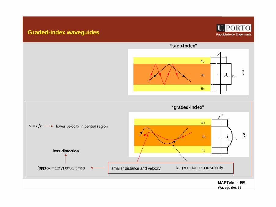
Faculdade de EngenhariaGraded-index waveguides
n1
n2
n2
y
n n1 n2
“step-index”
n1
n2
n2
y
n n1 n2
“graded-index”
ncv = lower velocity in central region
smaller distance and velocity larger distance and velocity(approximately) equal times
less distortion
MAPTele – EEWaveguides 89
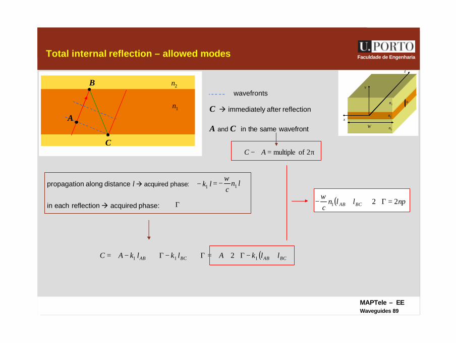
Faculdade de EngenhariaTotal internal reflection – allowed modes
W
z
y
x
b
2n
1n
2n
A
B
C
1n
2nwavefronts
C à immediately after reflection
A and C in the same wavefront
π=∠−∠ 2ofmultipleAC
Γ∠+−Γ∠+−∠=∠ BCAB lklkAC 11
propagation along distance là acquired phase:
in each reflectionà acquired phase: Γ∠
( )BCAB llkA +−Γ∠+∠= 12
lk1− lnc 1ω
−=
( ) πω
nllnc BCAB 221 =Γ∠++−
MAPTele – EEWaveguides 90
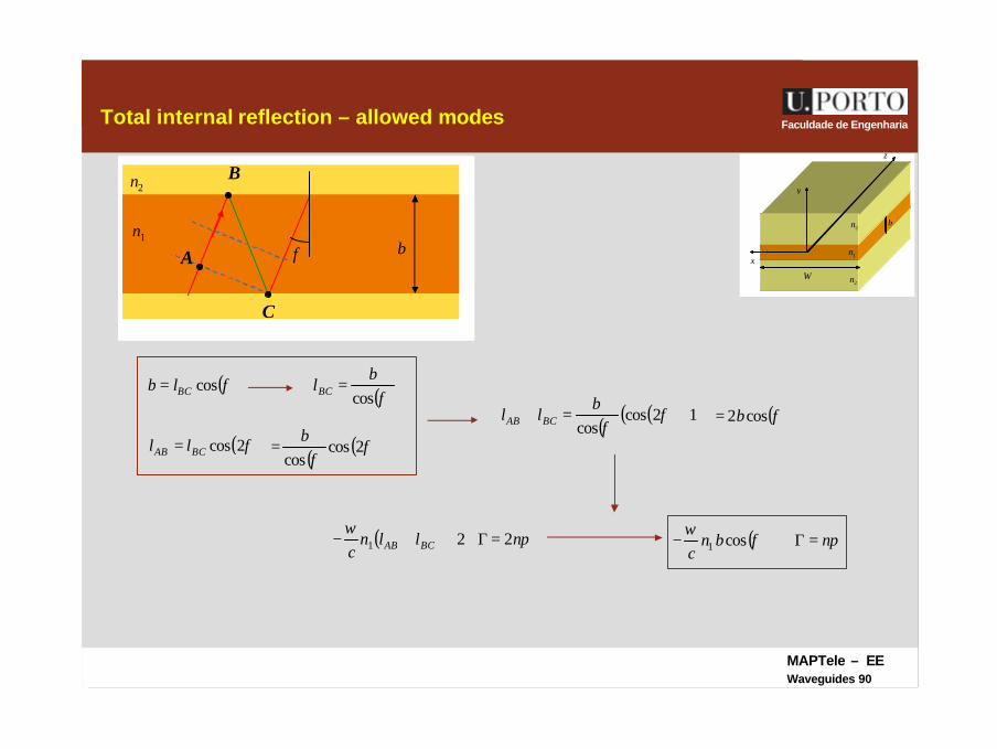
Faculdade de EngenhariaTotal internal reflection – allowed modes
W
z
y
x
b
2n
1n
2n
A
B
C
1n
2n
( )φcosBClb = ( )φcosb
lBC =
( )φ2cosBCAB ll =( ) ( )φφ
2coscos
b=
( ) ( )( )12coscos
+=+ φφ
bll BCAB ( )φcos2b=
bφ
( ) πω
nllnc BCAB 221 =Γ∠++− ( ) πφ
ωnbn
c=Γ∠+− cos1
MAPTele – EEWaveguides 91
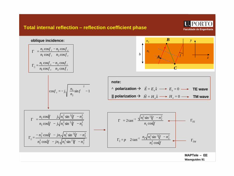
Faculdade de EngenhariaTotal internal reflection – reflection coefficient phase
A
B
C
1n
2n
b φ
oblique incidence:
ti
ti
nnnn
φφφφ
coscoscoscos
21
21
+−
=Γ⊥
it
it
nnnn
φφφφ
coscoscoscos
21
21| | +
−=Γ
1sincos2
2
1 −
−= φφ
nn
jt
( ) ( )( ) ( ) 2
222
11
22
2211
sincos
sincos
nnjn
nnjn
−−
−+=Γ⊥
φφ
φφ
( ) ( )( ) ( ) 2
222
1122
22
2211
22
| |sincos
sincos
nnjnn
nnjnn
−−
−−−=Γ
φφ
φφ
( )( )
−=Γ∠ −
⊥ φφ
cossin
tan21
22
2211
nnn
( )( )
−+=Γ∠ −
φ
φπ
cos
sintan2 2
2
22
22111
||n
nnn
note:
z
y
⊥ polarization à xEE x ˆ=r
0=zE TE wave
|| polarization à xHH x ˆ=r
0=zH TM wave
TEΓ∠
TMΓ∠
MAPTele – EEWaveguides 92
Faculdade de EngenhariaTotal internal reflection – equation for allowed modes
A
B
C
1n
2n
b φ
( )( )
−=Γ∠ −
φφ
cossin
tan21
22
2211
nnn
TE
( )( )
−+=Γ∠ −
φ
φπ
cos
sintan2 2
2
22
22111
n
nnnTM
z
y( ) πφ
ωnbn
c=Γ∠+− cos1
L,2,1=n
( )( ) modes TE,
cossin
tan2cos1
22
2211
1 π=
φ−φ
+φω
− − nn
nnbn
c
( )( )
( ) modes TM,1cos
sintan2cos 2
2
22
22111
1 π−=
φ
−φ+φ
ω− − n
n
nnnbn
c
propagating modes obey these equations
MAPTele – EEWaveguides 93
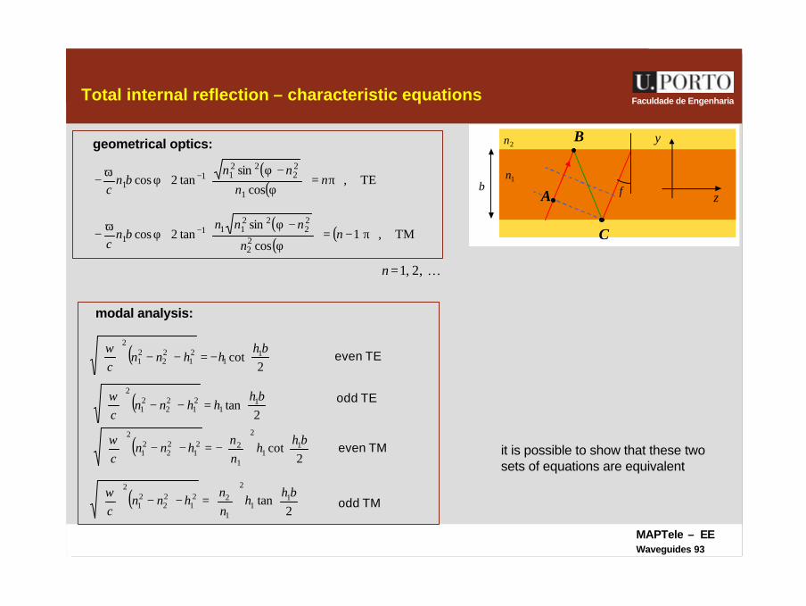
Faculdade de EngenhariaTotal internal reflection – characteristic equations
A
B
C
1n
2n
b φ z
y
( )( ) TE,
cos
sintan2cos
1
22
2211
1 π=
φ
−φ+φ
ω− − n
n
nnbn
c
( )( )
( ) TM,1cos
sintan2cos 2
2
22
22111
1 π−=
φ
−φ+φ
ω− − n
n
nnnbn
c
geometrical optics:
modal analysis:
( )
−=−−
2
cot 11
2
1
221
22
21
2 bhh
nn
hnncω
( )
−=−−
2cot 1
121
22
21
2 bhhhnn
cω
( )
=−−
2
tan 11
2
1
221
22
21
2 bhh
nn
hnncω
( )
=−−
2tan 1
121
22
21
2 bhhhnn
cω
K,2,1=n
even TM
even TE
odd TM
odd TE
it is possible to show that these two sets of equations are equivalent
MAPTele – EEWaveguides 94
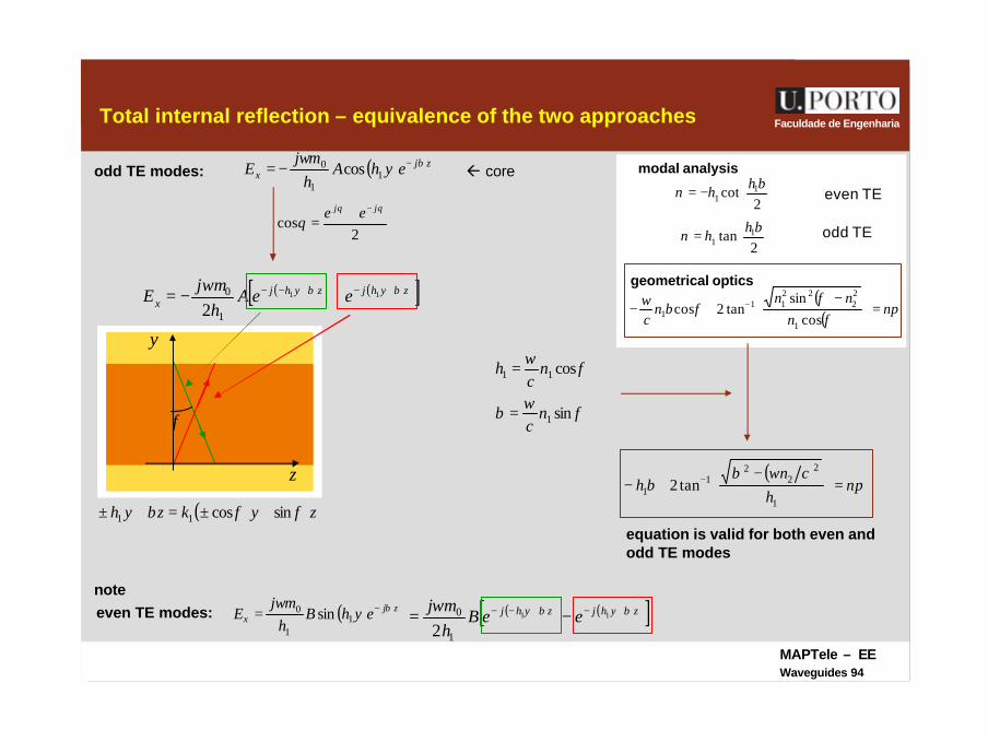
Faculdade de Engenharia
z
y
Total internal reflection – equivalence of the two approaches
−=
2cot 1
1bhhν
=
2tan 1
1bhhν
even TE
odd TE
( )( ) πφ
φφω n
nnn
bnc
=
−+− −
cossin
tan2cos1
22
2211
1
geometrical optics
modal analysisß coreodd TE modes: ( ) zjx eyhA
hj
E βωµ −−= 11
0 cos
( ) ( )[ ]zyhjzyhjx eeA
hj
E ββωµ +−+−− +−= 11
1
0
2
2cos
θθ
θjj ee −+
=
φ
( )zykzyh φφβ sincos11 +±=+±
φωβ
φω
sin
cos
1
11
nc
nc
h
=
=
( )π
ωβn
h
cnbh =
−+− −
1
22
21
1 tan2
even TE modes:note
( ) zjx eyhB
hj
E βωµ −= 11
0 sin ( ) ( )[ ]zyhjzyhj eeBh
j ββωµ +−+−− −= 11
1
0
2
equation is valid for both even andodd TE modes
MAPTele – EEWaveguides 95
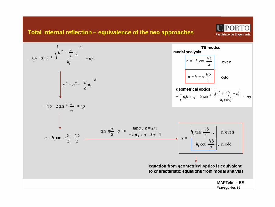
Faculdade de EngenhariaTotal internal reflection – equivalence of the two approaches
−=
2cot 1
1bhhν
=
2tan 1
1bhhν
even
odd
( )( ) πφ
φφω n
nnn
bnc
=
−+− −
cossin
tan2cos1
22
2211
1
geometrical optics
modal analysisTE modes
π
ωβ
nh
nc
bh =
−
+− −
1
2
22
11 tan2
πν
nh
bh =
+− −
1
11 tan2
2
222
−= n
cω
βν
+=
22tan 1
1bh
nhπ
ν
+=−=
=
+
12,cot2,tan
2tan
mnmn
nθθ
θπ
−
=νoddn,
2cot
evenn,2
tan
11
11
bhh
bhh
equation from geometrical optics is equivalentto characteristic equations from modal analysis
MAPTele – EEWaveguides 96
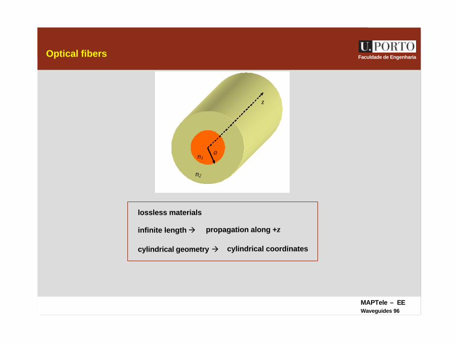
Faculdade de EngenhariaOptical fibers
z
n1 a
n2
lossless materials
infinite length à propagation along +z
cylindrical geometry à cylindrical coordinates
MAPTele – EEWaveguides 97
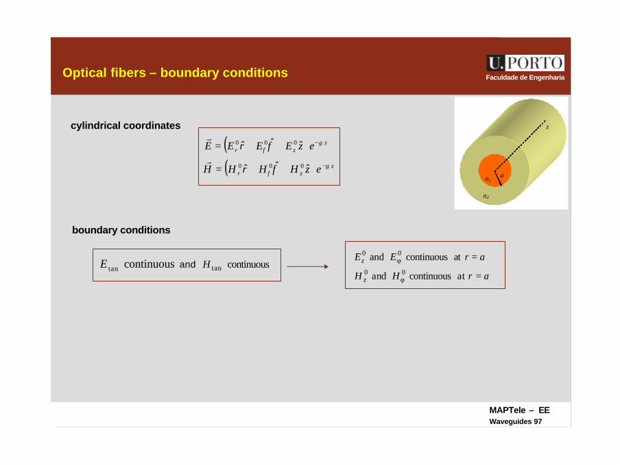
Faculdade de EngenhariaOptical fibers – boundary conditions
z
n1 a
n2
continuoustanE continuoustanHand
boundary conditions
arHH
arEE
z
z
=
=
φ
φ
atcontinuousnda
tacontinuousand00
00
cylindrical coordinates
( ) zzr ezEErEE γ
φ φ −++= ˆˆˆ 000r
( ) zzr ezHHrHH γ
φ φ −++= ˆˆˆ 000r
MAPTele – EEWaveguides 98
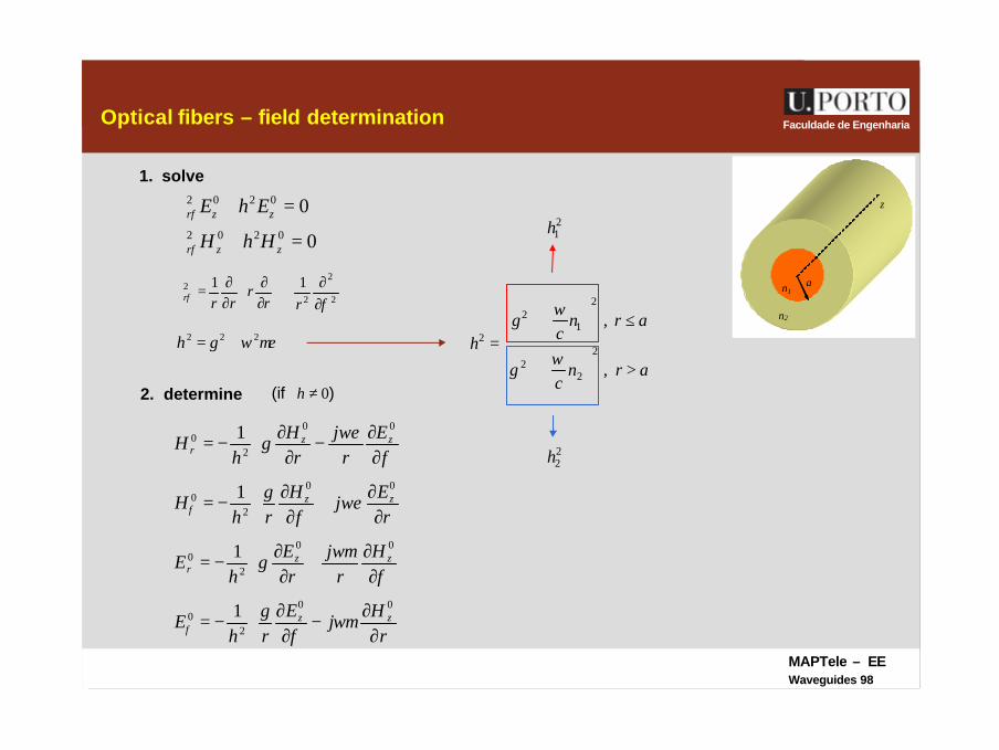
Faculdade de EngenhariaOptical fibers – field determination
z
n1 a
n2
(if )0≠h2. determine
µεωγ 222 +=h
1. solve
0
00202
0202
=+∇
=+∇
zzr
zzr
HhH
EhE
φ
φ
2
2
22 11
φφ ∂∂+
∂∂
∂∂=∇
rrr
rrr
∂
∂−∂
∂−=
∂
∂+∂
∂−=
∂
∂+∂
∂−=
∂∂−
∂∂−=
rHjE
rhE
Hr
jr
Eh
E
rEjH
rhH
Er
jr
Hh
H
zz
zzr
zz
zzr
00
20
00
20
00
20
00
20
1
1
1
1
ωµφ
γ
φωµγ
ωεφ
γ
φωεγ
φ
φ
>
+
≤
+
=
arnc
arnch
,
,
2
22
2
12
2
ωγ
ωγ
21h
22h
MAPTele – EEWaveguides 99
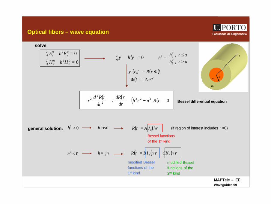
Faculdade de EngenhariaOptical fibers – wave equation
z
n1 a
n2
solve
0
00202
0202
=+∇
=+∇
zzr
zzr
HhH
EhE
φ
φ
>≤
=arharh
h,,
22
212022 =+∇ ψψφ hr
( ) ( ) ( )φφψ Φ= rRr ,
( ) φφ jnAe=Φ
( ) ( ) ( ) ( ) 02222
22 =−++ rRnrh
drrdR
rdr
rRdr Bessel differential equation
general solution: ( ) ( )hrJArR n= (if region of interest includes r =0) 02 >h realh
02 <h νjh = ( ) ( ) ( )rCKrIBrR nn νν +=
Bessel functionsof the 1st kind
modified Besselfunctions of the1st kind
modified Besselfunctions of the2nd kind
MAPTele – EEWaveguides 100
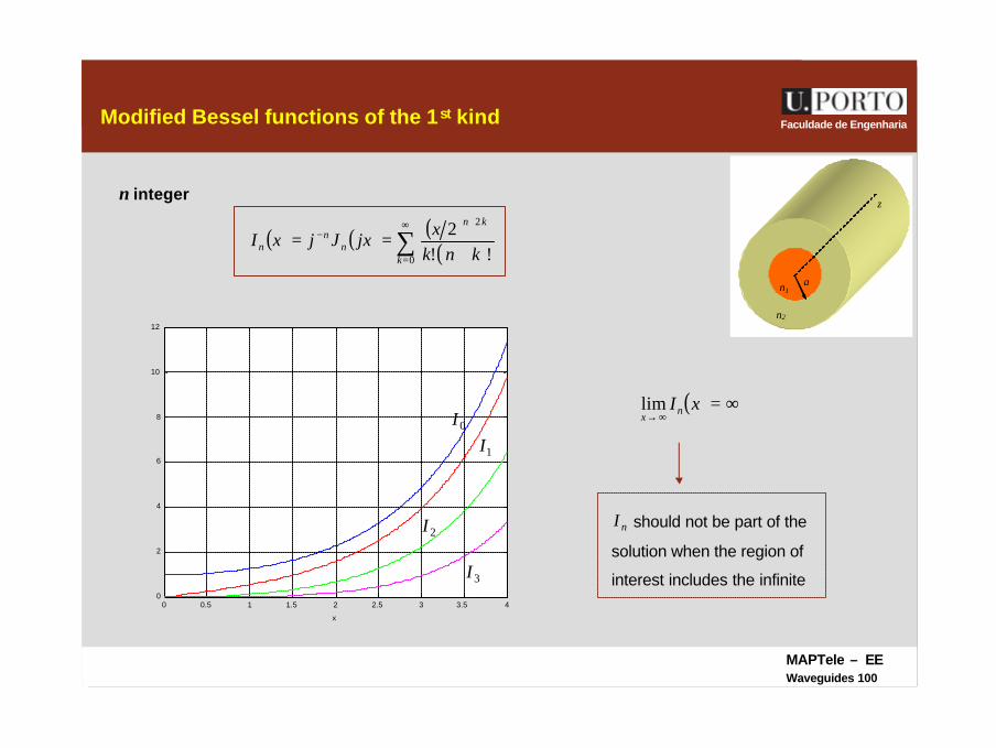
Faculdade de EngenhariaModified Bessel functions of the 1st kind
z
n1 a
n2
n integer
( ) ( ) ( )( )∑
∞
=
+−
+==
0
2
!!2
k
kn
nn
n knkxjxJjxI
0 0.5 1 1.5 2 2.5 3 3.5 40
2
4
6
8
10
12
x
0I
1I
2I
3I
( ) ∞=∞→
xInxlim
should not be part of the
solution when the region of
interest includes the infinite
nI
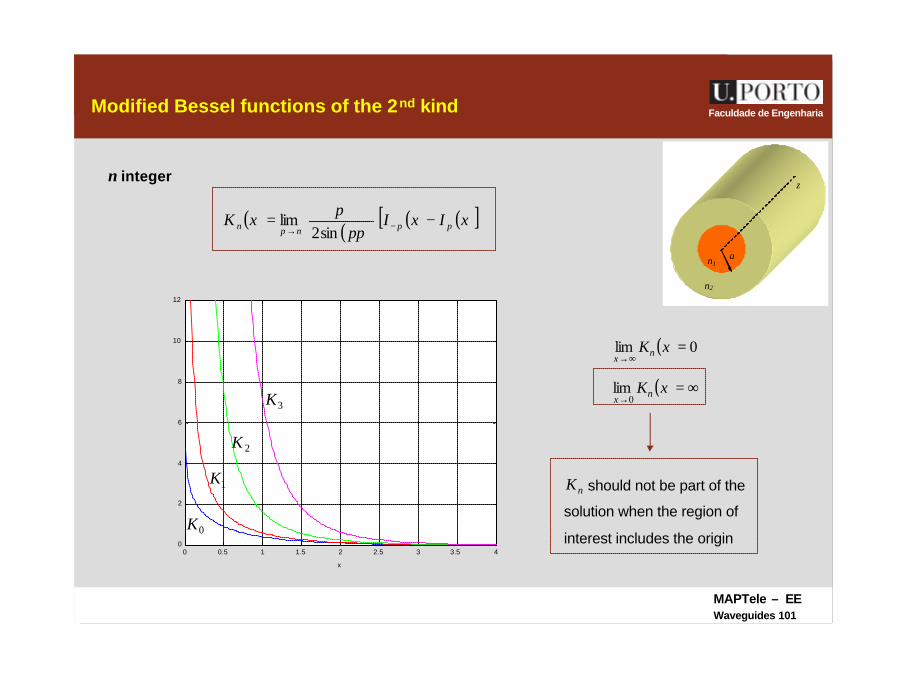
MAPTele – EEWaveguides 101
Faculdade de Engenharia
0 0.5 1 1.5 2 2.5 3 3.5 40
2
4
6
8
10
12
x
Modified Bessel functions of the 2nd kind
z
n1 a
n2
n integer
0K
1K
2K
3K( ) ∞=
→xKnx 0
lim
should not be part of the
solution when the region of
interest includes the origin
nK
( ) ( ) ( ) ( )[ ]xIxIp
xK ppnpn −= −→ ππ
sin2lim
( ) 0lim =∞→
xKnx
MAPTele – EEWaveguides 102
Faculdade de EngenhariaSolution of the wave equation
z
n1 a
n2
( ) ( )hrJArR n=realh
νjh = ( ) ( ) ( )rCKrIBrR nn νν +=
( ) ( ) ( )φφψ Φ= rRr ,
( ) φφ jnAe=Φ
∞=∞→rlim ∞=→0lim r
guided wave àreal1h
νjh =2
( ) ( )( )
>≤
=arerBK
arerhAJr
jnn
jnn
,
,, 1
φ
φ
νφψ
( ) 21
22
21
2
hnnc
−−
=
ων
22
221
2
1 νωω
β +
=−
= n
chn
c
21 nc
nc
ωβ
ω>> 21 nn >
0lim =∞→r
MAPTele – EEWaveguides 103
Faculdade de EngenhariaLongitudinal components
z
n1 a
n2
( ) ( ) ( )φφψ Φ= rRr ,
( ) φφ jnAe=Φ
cladding
( ) ( )( )
>≤
=arerBK
arerhAJr
jnn
jnn
,
,, 1
φ
φ
νφψ
( )( ) φ
φ
jnnz
jnnz
erhBJH
erhAJE
10
10
=
=core
( )( ) φ
φ
ν
νjn
nz
jnnz
erDKH
erCKE
=
=0
0
TM modes à 00 =zH
TE modes à 00 =zE
HE and EH modes à 0and0 00 ≠≠ zz HE
note:
hybrid modes
MAPTele – EEWaveguides 104
Faculdade de EngenhariaTransverse components
z
n1 a
n2
( )( ) φ
φ
jnnz
jnnz
erhBJH
erhAJE
10
10
=
=
∂
∂−
∂∂
−=
∂
∂+∂
∂−=
∂
∂+
∂∂
−=
∂
∂−
∂∂
−=
rH
jE
rhE
Hr
jr
Eh
E
rE
jH
rhH
Er
jr
Hh
H
zz
zzr
zz
zzr
00
20
00
20
00
20
00
20
1
1
1
1
ωµφ
γ
φωµγ
ωεφ
γ
φωε
γ
φ
φ
1hh =
φωεβ jn
nnr erhAJr
nrhBJhj
hH
+−= )()('1
11
1121
0
φφ ωε
β jnnn erhAJhjrhBJ
rn
hH
+−−= )(')(1
111121
0
φωµβ jn
nnr erhBJr
nrhAJhj
hE
−−= )()('1
10
1121
0
φφ ωµ
β jnnn erhBJhjrhAJ
rn
hE
−−−= )(')(1
110121
0
νjh =( )( ) φ
φ
ν
νjn
nz
jnnz
erDKH
erCKE
=
=0
0
φνωενβνν
jnnnr erCK
rnrDKjH
+= )()('1 2
20
φφ ννωενβ
νjn
nn erCKjrDKrnH
+−= )(')(1
220
φνωµ
νβνν
jnnnr erDK
rn
rCKjE
−= )()('1 0
20
φφ ννωµνβ
νjn
nn erDKjrCKrnE
−−= )(')(1
020
cladding
core
MAPTele – EEWaveguides 105
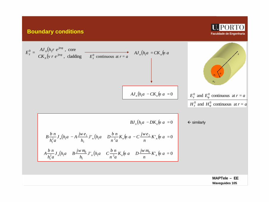
Faculdade de EngenhariaBoundary conditions
z
n1 a
n2
arHH
arEE
z
z
=
=
φ
φ
at continuousnda
at continuousand00
00
( ) ( ) ( ) ( ) 0'' 021
1
012
1
=+++ aKj
DaKan
CahJh
jBahJ
ahn
A nnnn νν
µων
νβµωβ
( )( )
ν= φ
φ
cladding, core,10
jnn
jnn
z erCKerhAJ
E ( ) ( )aCKahAJ nn ν=1arE z =at continuous0
( ) ( ) 01 =− aCKahAJ nn ν
ß similarly( ) ( ) 01 =− aDKahBJ nn ν
( ) ( ) ( ) ( ) 0'' 221
1
112
1
=−+− aKj
CaKan
DahJh
jAahJ
ahn
B nnnn νν
εων
νβεωβ
MAPTele – EEWaveguides 106
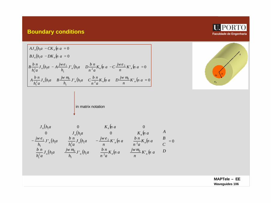
Faculdade de EngenhariaBoundary conditions
z
n1 a
n2 ( ) ( ) ( ) ( ) 0'' 0
211
012
1
=+++ aKj
DaKan
CahJh
jBahJ
ahn
A nnnn νν
µων
νβµωβ
( ) ( ) 01 =− aCKahAJ nn ν
in matrix notation
( ) ( ) 01 =− aDKahBJ nn ν
( ) ( ) ( ) ( ) 0'' 221
1
112
1
=−+− aKj
CaKan
DahJh
jAahJ
ahn
B nnnn νν
εων
νβεωβ
( ) ( )( ) ( )
( ) ( ) ( ) ( )
( ) ( ) ( ) ( )
0
''
''
0000
021
1
012
1
22
121
11
1
1
1
=
−−
D
CB
A
aKj
aKan
ahJh
jahJ
ahn
aKan
aKj
ahJahn
ahJh
jaKahJ
aKahJ
nnnn
nnnn
nn
nn
νν
µων
νβµωβ
ννβ
νν
εωβεων
ν
MAPTele – EEWaveguides 107
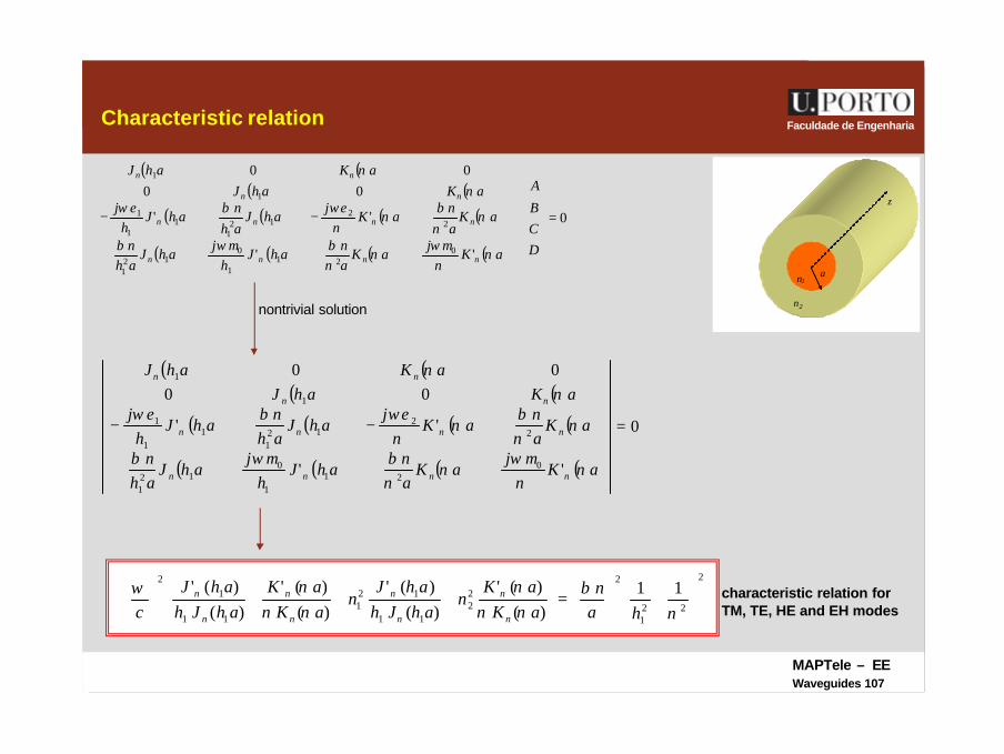
Faculdade de EngenhariaCharacteristic relation
z
n1 a
n2 nontrivial solution
( ) ( )( ) ( )
( ) ( ) ( ) ( )
( ) ( ) ( ) ( )
0
''
''
0000
021
1
012
1
22
121
11
1
1
1
=
−−
DCB
A
aKj
aKan
ahJh
jahJ
ahn
aKan
aKj
ahJahn
ahJh
jaKahJ
aKahJ
nnnn
nnnn
nn
nn
νν
µων
νβµωβ
ννβ
νν
εωβεων
ν
( ) ( )( ) ( )
( ) ( ) ( ) ( )
( ) ( ) ( ) ( )
0
''
''
0000
021
1
012
1
22
121
11
1
1
1
=−−
aKj
aKan
ahJh
jahJ
ahn
aKan
aKj
ahJahn
ahJh
jaKahJ
aKahJ
nnnn
nnnn
nn
nn
νν
µων
νβµωβ
ννβ
νν
εωβεων
ν
2
221
222
11
121
11
12
11)()('
)()('
)()('
)()('
+
=
+
+
νβ
ννν
νννω
han
aKaK
nahJh
ahJn
aKaK
ahJhahJ
c n
n
n
n
n
n
n
n characteristic relation forTM, TE, HE and EH modes
MAPTele – EEWaveguides 108
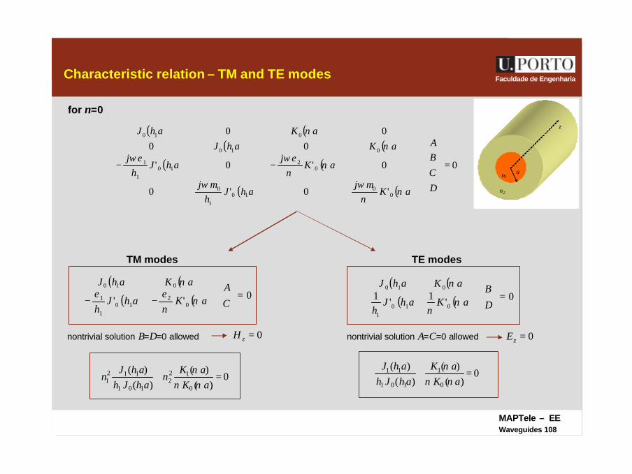
Faculdade de EngenhariaCharacteristic relation – TM and TE modes
z
n1 a
n2
for n=0
( ) ( )( ) ( )
( ) ( )
( ) ( )
0
'0'0
0'0'
0000
00
101
0
02
101
1
010
010
=
−−
DCBA
aKj
ahJh
j
aKj
ahJh
jaKahJ
aKahJ
νν
µωµω
νν
εωεων
ν
( ) ( )( ) ( ) 0'' 0
210
1
1
010
=
−− C
AaKahJ
h
aKahJ
ννεε
ν ( ) ( )( ) ( ) 0'1'1
0101
010
=
D
BaKahJ
h
aKahJ
νν
ν
nontrivial solution B=D=0 allowed
TM modes
nontrivial solution A=C=0 allowed
TE modes
0=zH 0=zE
0)(
)()(
)(
0
122
101
1121 =+
aKaK
nahJh
ahJn
ννν 0
)()(
)()(
0
1
101
11 =+aK
aKahJh
ahJνν
ν
MAPTele – EEWaveguides 109
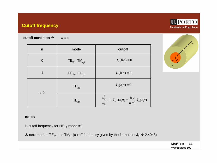
Faculdade de EngenhariaCutoff frequency
z
n1 a
n2
cutoff condition à 0=ν
0)( 10 =ahJ
0)( 11 =ahJ
0)( 1 =ahJn
)(1
)(1 11
1122
21 ahJ
nah
ahJnn
nn −=
+ −HEnp
EHnp
≥ 2
HE1p EH1p1
TE0p TM0p0
cutoffmoden
notes
1. cutoff frequency for HE11 mode =0
2. next modes: TE01 and TM01 (cutoff frequency given by the 1st zero of J0 à 2.4048)
MAPTele – EEWaveguides 110
Faculdade de EngenhariaNormalized frequency
z
n1 a
n2
normalized frequency(V parameter)
( ) 2221
2 ahV ν+= ( )22
21
2
nnca
−
=
ω
2
122
1
+= n
ch
ωγ
2
222
−−= n
cω
γν
22
21
0
2 nnaV −=λπ
cutoff à 0=ν ( ) ( )cut1cut ahV =
wavelength in vacuum
011 =→ cfHE
4048.2and 10101 >→ ahTETM
single mode à 4048.2<V
multimode à 4048.2>V
note
propagation of
MAPTele – EEWaveguides 111
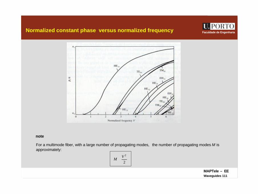
Faculdade de EngenhariaNormalized constant phase versus normalized frequency
For a multimode fiber, with a large number of propagating modes, the number of propagating modes M is approximately:
note
2
2VM ≅