Water Flow in Pipes -...
27
Chapter (3) Water Flow in Pipes
Transcript of Water Flow in Pipes -...
Chapter (3)
Water Flow in
Pipes
Page (2)
Water Flow in Pipes Hydraulics
Dr.Khalil Al-astal Eng. Ahmed Al-Agha Eng. Ruba Awad
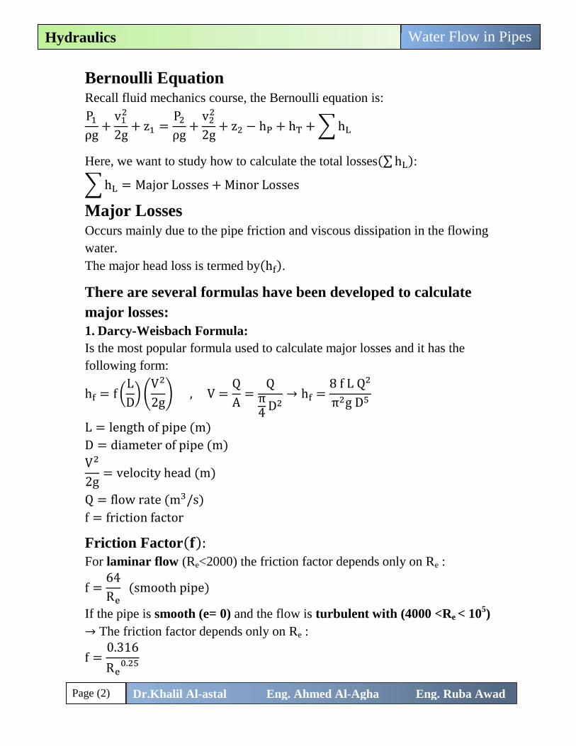
Bernoulli Equation Recall fluid mechanics course, the Bernoulli equation is:
P1
ρg+
v12
2g+ z1 =
P2
ρg+
v22
2g+ z2 − hP + hT + ∑ hL
Here, we want to study how to calculate the total losses(∑ hL):
∑ hL = Major Losses + Minor Losses
Major Losses Occurs mainly due to the pipe friction and viscous dissipation in the flowing
water.
The major head loss is termed by(hf).
There are several formulas have been developed to calculate
major losses:
1. Darcy-Weisbach Formula:
Is the most popular formula used to calculate major losses and it has the
following form:
hf = f (L
D) (
V2
2g) , V =
Q
A=
Qπ4
D2→ hf =
8 f L Q2
π2g D5
L = length of pipe (m)
D = diameter of pipe (m)
V2
2g= velocity head (m)
Q = flow rate (m3/s)
f = friction factor
Friction Factor(𝐟): For laminar flow (Re<2000) the friction factor depends only on Re :
f =64
Re (smooth pipe)
If the pipe is smooth (e= 0) and the flow is turbulent with (4000 <Re < 105)
→ The friction factor depends only on Re :
f =0.316
Re0.25
Page (3)
Water Flow in Pipes Hydraulics
Dr.Khalil Al-astal Eng. Ahmed Al-Agha Eng. Ruba Awad
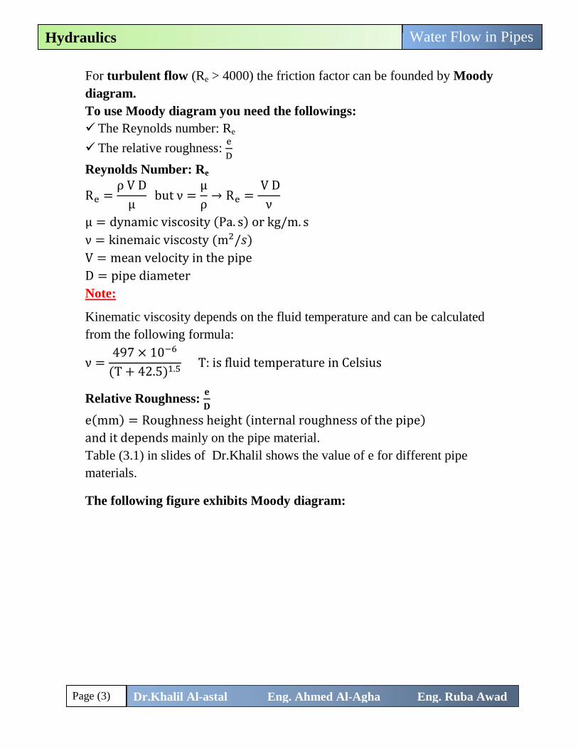
For turbulent flow (Re > 4000) the friction factor can be founded by Moody
diagram.
To use Moody diagram you need the followings:
The Reynolds number: Re
The relative roughness: e
D
Reynolds Number: Re
Re =ρ V D
μ but ν =
μ
ρ→ Re =
V D
ν
μ = dynamic viscosity (Pa. s) or kg/m. s
ν = kinemaic viscosty (m2/𝑠)
V = mean velocity in the pipe
D = pipe diameter
Note:
Kinematic viscosity depends on the fluid temperature and can be calculated
from the following formula:
ν =497 × 10−6
(T + 42.5)1.5 T: is fluid temperature in Celsius
Relative Roughness: 𝐞
𝐃
e(mm) = Roughness height (internal roughness of the pipe)
and it depends mainly on the pipe material.
Table (3.1) in slides of Dr.Khalil shows the value of e for different pipe
materials.
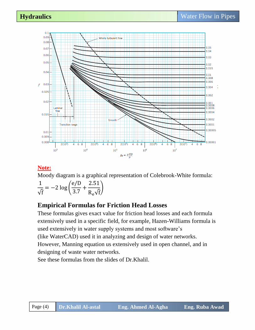
The following figure exhibits Moody diagram:
Page (4)
Water Flow in Pipes Hydraulics
Dr.Khalil Al-astal Eng. Ahmed Al-Agha Eng. Ruba Awad
Note:
Moody diagram is a graphical representation of Colebrook-White formula:
1
√f= −2 log (
e/D
3.7+
2.51
Re√f)
Empirical Formulas for Friction Head Losses
These formulas gives exact value for friction head losses and each formula
extensively used in a specific field, for example, Hazen-Williams formula is
used extensively in water supply systems and most software’s
(like WaterCAD) used it in analyzing and design of water networks.
However, Manning equation us extensively used in open channel, and in
designing of waste water networks.
See these formulas from the slides of Dr.Khalil.
Page (5)
Water Flow in Pipes Hydraulics
Dr.Khalil Al-astal Eng. Ahmed Al-Agha Eng. Ruba Awad
Minor Losses Occurs due to the change of the velocity of the flowing fluid in the
magnitude or in the direction.
So, the minor losses at:
Valves.
Tees.
Bends.
Contraction and Expansion.
The minor losses are termed by(hm) and have a common form:
hm = KL
V2
2g
KL = minor losses coefficient and it depends on the type of fitting
Minor Losses Formulas
Minor Losses
Entrance of a pipe: hent = KentrV2
2g Exit of a pipe: hexit = Kexit
V2
2g
Sudden Contraction: hsc = KscV2
2
2g
Sudden Expansion: hse = KseV1
2
2g
or hse =(V1 − V2)2
2g
Gradual Enlargement: hge = Kge(V1
2−V22)
2g Gradual Contraction: 𝐡𝐠𝐜 = 𝐊𝐠𝐜
(𝐕𝟐𝟐−𝐕𝟏
𝟐)
𝟐𝐠
Bends in pipes: hbend = KbendV2
2g Pipe Fittings: hv = Kv
V2
2g
The value of (K) for each fitting can be estimated from tables exist in slides
of Dr.Khalil.
You must save the following values of K:
For sharp edge entrance: K = 0.5
For all types of exists: K = 1.
Page (6)
Water Flow in Pipes Hydraulics
Dr.Khalil Al-astal Eng. Ahmed Al-Agha Eng. Ruba Awad
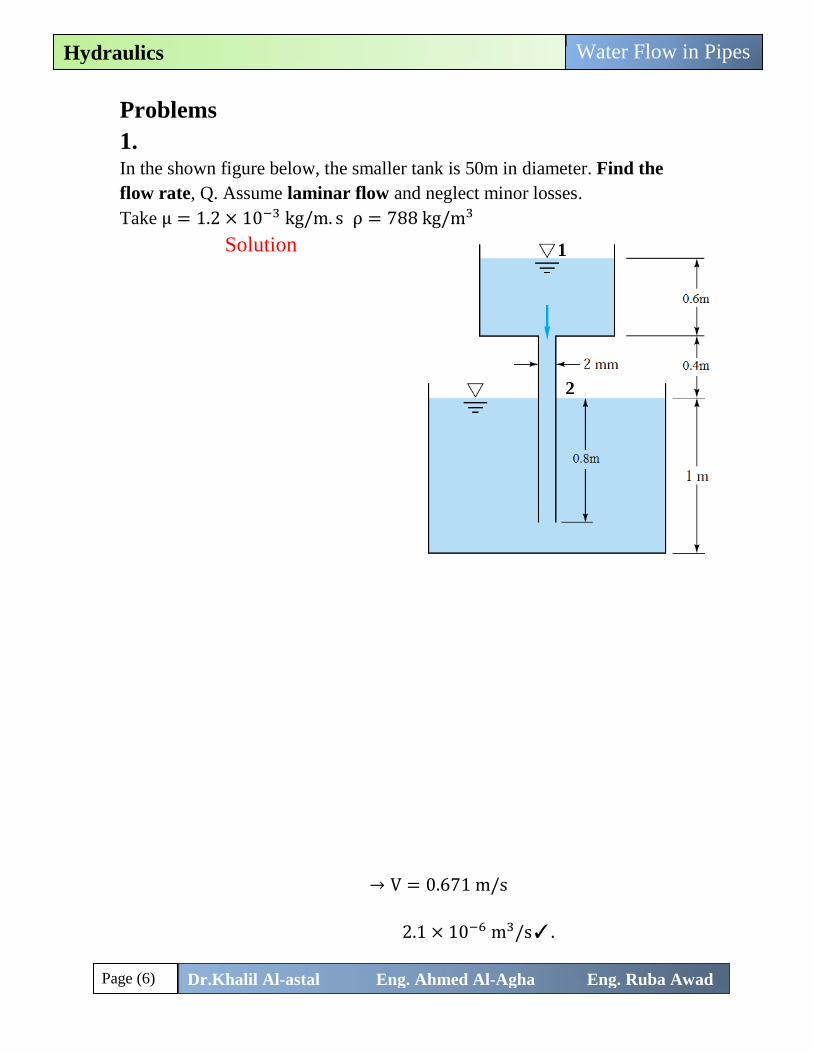
Problems
1. In the shown figure below, the smaller tank is 50m in diameter. Find the
flow rate, Q. Assume laminar flow and neglect minor losses.
Take μ = 1.2 × 10⁻³ kg/m. s ρ = 788 kg/m3
Solution
For laminar f =64
Re
Re =ρ V D
μ=
788 × 2 × 10−3 × V
1.2 × 10⁻³
→ Re = 1313.33 V (substitute in f)
f =64
Re=
64
1313.33 V=
0.0487
V≫ (1)
Now by applying Bernoulli’s
equation from the free surface of
upper to lower reservoir
(Points 1 and 2).
P1
ρg+
v12
2g+ z1 =
P2
ρg+
v22
2g+ z2 + ∑ hL
P1 = P2 = V1 = V2 = 0.0
Assume the datum at point (2) →
0 + 0 + (0.4 + 0.6) = 0 + 0 + 0 + ∑ hL → ∑ hL = 1m
∑ hL = 1m = hf in the pipe that transport fluid from reservoir 1 to 2
hf = f (L
D) (
V2
2g) L = (0.4 + 0.8) = 1.2m , D = 0.002m
1 = f (1.2
0.002) (
V2
19.62) ≫ 2 → Substitute from (1)in (2) →
1 =0.0487
V× (
1.2
0.002) (
V2
19.62) → V = 0.671 m/s
Q = A × V =π
4× 0.0022 × 0.671 = 2.1 × 10⁻⁶ m3/s✓.
1
2
Page (7)
Water Flow in Pipes Hydraulics
Dr.Khalil Al-astal Eng. Ahmed Al-Agha Eng. Ruba Awad
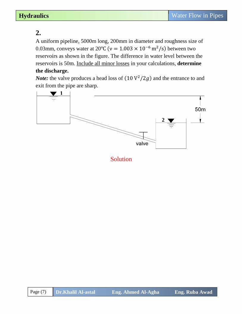
2. A uniform pipeline, 5000m long, 200mm in diameter and roughness size of
0.03mm, conveys water at 20℃ (ν = 1.003 × 10⁻⁶ m2/s) between two
reservoirs as shown in the figure. The difference in water level between the
reservoirs is 50m. Include all minor losses in your calculations, determine
the discharge.
Note: the valve produces a head loss of (10 V2/2𝑔) and the entrance to and
exit from the pipe are sharp.
Solution
Applying Bernoulli’s equation between the two reservoirs
P1
ρg+
v12
2g+ z1 =
P2
ρg+
v22
2g+ z2 + ∑ hL
P1 = P2 = V1 = V2 = 0.0
Assume the datum at lower reservoir (point 2) →
0 + 0 + 50 = 0 + 0 + 0 + ∑ hL → ∑ hL = 50m
∑ hL = hf + hm = 50
Major Losses:
hf = f (L
D) (
V2
2g) = hf = f × (
5000
0.2) (
V2
19.62) = 1274.21 f V2
Minor losses:
For Entrance:
hent = Kentr
V2
2g (For sharp edge entrance, the value ofKentr = 0.5) →
2
1
Page (8)
Water Flow in Pipes Hydraulics
Dr.Khalil Al-astal Eng. Ahmed Al-Agha Eng. Ruba Awad
hent = 0.5 ×V2
19.62= 0.0255 V2
For Exit:
hexit = Kexit
V2
2g (For exit: Kexit = 1) →
hexit = 1 ×V2
19.62= 0.051 V2
For Valve:
hvalve = 10 ×V2
2g= 0.51V2
hm = (0.0255 + 0.051 + 0.51)V2 = 0.5865 V2
∑ hL = 1274.21 f V2 + 0.5865 V2 = 50 → V2 =50
1274.21 f + 0.5865> (1)
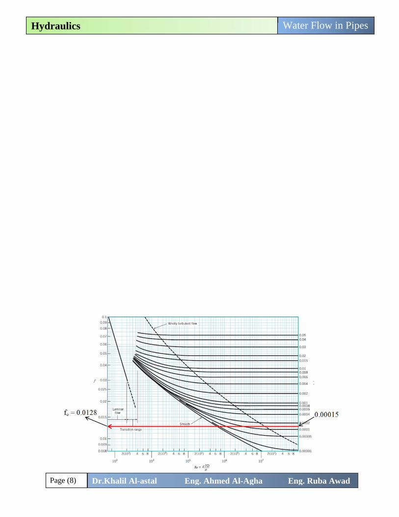
e
D=
0.03
200= 0.00015
In all problems like this (flow rate or velocity is unknown), the best initial
value for f can be found as following:
Draw a horizontal line (from left to right) starts from the value of e
D till
intercept with the vertical axis of the Moody chart and the initial f value is
the intercept as shown in the following figure:
Page (9)
Water Flow in Pipes Hydraulics
Dr.Khalil Al-astal Eng. Ahmed Al-Agha Eng. Ruba Awad
So as shown in the above figure, the initial value of f = 0.0128
Substitute in Eq. (1) → V2 =50
1274.21 × 0.0128 + 0.5865= 2.96
→ V = 1.72 m/s
→ Re = V D
ν=
1.72 × 0.2
1.003 × 10−6 = 3.4 × 10⁵ and
e
D= 0.00015 → Moody
f = 0.016 → Substitute in Eq. (1) → V = 1.54 → Re = 3.1 × 10⁵
→ Moody → f ≅ 0.016
So, the velocity is V = 1.54 m/s
Q = A × V =π
4× 0.22 × 1.54 = 0.0483 m3/s ✓.
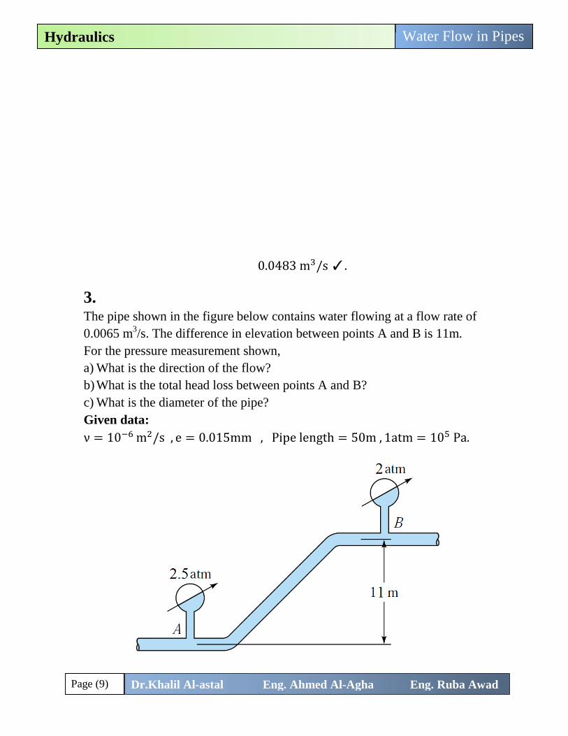
3. The pipe shown in the figure below contains water flowing at a flow rate of
0.0065 m3/s. The difference in elevation between points A and B is 11m.
For the pressure measurement shown,
a) What is the direction of the flow?
b) What is the total head loss between points A and B?
c) What is the diameter of the pipe?
Given data:
ν = 10−6 m2/s , e = 0.015mm , Pipe length = 50m , 1atm = 105 Pa.
Page (10)
Water Flow in Pipes Hydraulics
Dr.Khalil Al-astal Eng. Ahmed Al-Agha Eng. Ruba Awad
Solution
a) Direction of flow??
To know the direction of flow, we calculate the total head at each point, and
then the fluid will moves from the higher head to lower head.
Assume the datum is at point A:
Total head at point A:
PA
ρg+
vA2
2g+ zA =
2.5 × 10⁵
9810+
vA2
2g+ 0 = 25.484 +
vA2
2g
Total head at point BA:
PB
ρg+
vB2
2g+ zB =
2 × 10⁵
9810+
vB2
2g+ 11 = 31.39 +
vB2
2g
But, VA = VB (Since there is the same diameter and flow at A and B)
So, the total head at B is larger than total head at A>> the water is flowing
from B (upper) to A (lower) ✓.
b) Head loss between A and B??
Apply Bernoulli’s equation between B and A (from B to A)
PB
ρg+
vB2
2g+ zB =
PA
ρg+
vA2
2g+ zA + ∑ hL
31.39 +vB
2
2g= 25.484 +
vA2
2g+ ∑ hL , But VA = VB → ∑ hL = 5.9 m✓.
c) Diameter of the pipe??
∑ hL = hf + hm = 5.9m (no minor losses) → ∑ hL = hf = 5.9m
hf = f (L
D) (
V2
2g)
5.9 = f (50
D) × (
V2
19.62)
V =Q
A=
0.0065π4
× D2=
0.00827
D2→ V2 =
6.85 × 10⁻⁵
D4→
5.9 = f (50
D) × (
6.85 × 10⁻⁵
19.62 D4) → 5.9 = f ×
0.000174
D5
Page (11)
Water Flow in Pipes Hydraulics
Dr.Khalil Al-astal Eng. Ahmed Al-Agha Eng. Ruba Awad
→ D5 = 2.96 × 10⁻⁵ f → D = (2.96 × 10⁻⁵)15 × f
15 → D = 0.124 f
15
Re = 0.00827
D2 × D
10−6=
0.00827
10−6 D
Now, assume the initial value for f is 0.02 (random guess)
→ D = 0.124 × 0.0215 = 0.0567 m → Re =
0.00827
10−6 × 0.0567= 1.46 × 10⁵
→e
D=
0.015
56.7= 0.00026 → Moody → f ≅ 0.019
→ D = 0.124 × 0.01915 = 0.056 m → Re =
0.00827
10−6 × 0.056= 1.47 × 10⁵
→e
D=
0.015
56= 0.00027 → Moody → f ≅ 0.019
So, the diameter of the pipe is 0.056 m = 56 mm ✓.
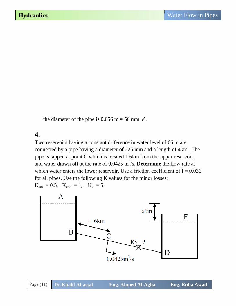
4. Two reservoirs having a constant difference in water level of 66 m are
connected by a pipe having a diameter of 225 mm and a length of 4km. The
pipe is tapped at point C which is located 1.6km from the upper reservoir,
and water drawn off at the rate of 0.0425 m3/s. Determine the flow rate at
which water enters the lower reservoir. Use a friction coefficient of f = 0.036
for all pipes. Use the following K values for the minor losses:
Kent = 0.5, Kexit = 1, Kv = 5

Page (12)
Water Flow in Pipes Hydraulics
Dr.Khalil Al-astal Eng. Ahmed Al-Agha Eng. Ruba Awad
Solution
Applying Bernoulli’s equation between points A and E:
PA
ρg+
vA2
2g+ zA =
PE
ρg+
vE2
2g+ zE + ∑ hL
PA = PE = VA = VE = 0.0
Assume the datum at point E →
0 + 0 + 66 = 0 + 0 + 0 + ∑ hL → ∑ hL = 66m
∑ hL = hf + hm = 66
Major Losses:
Since the pipe is tapped, we will divide the pipe into two parts with the same
diameter ; (1) 1.6 km length from B to C, and (2) 2.4 km length from C to D.
hf = f (L
D) (
V2
2g)
For part (1)
hf,1 = 0.036 × (1600
0.225) (
V12
19.62) = 13.05 V1
2
For part (2)
hf,2 = 0.036 × (2400
0.225) (
V22
19.62) = 19.6 V2
2
hf = 13.05 V12 + 19.6 V2
2
Minor losses:
For Entrance: (due to part 1)
hent = Kentr
V12
2g (Kentr = 0.5) →
hent = 0.5 ×V1
2
19.62= 0.0255 V1
2
For Exit: (due to part 2)
hexit = Kexit
V22
2g ( Kexit = 1) →

Page (13)
Water Flow in Pipes Hydraulics
Dr.Khalil Al-astal Eng. Ahmed Al-Agha Eng. Ruba Awad
hexit = 1 ×V2
2
19.62= 0.051 V2
2
For Valve: (valve exists in part 2)
hvalve = 5 ×V2
2
2g= 0.255V2
2
hm = 0.0255 V12 + 0.051 V2
2+0.255V22 = 0.0255 V1
2 + 0.306V22
∑ hL = (13.05 V12 + 19.6 V2
2) + (0.0255 V12 + 0.306V2
2) = 66
→ 66 = 13.0755 V12 + 19.906 V2
2 ≫ Eq. (1)
Continuity Equation: π
4× 0.2252 × V1 = 0.0425 +
π
4× 0.2252 × V2
V1 = 1.068 + V2 (substitute in Eq. (1)) →
66 = 13.0755 (1.068 + V2)2 + 19.906 V22 → V2 = 0.89 m/s
Q2 =π
4× 0.2252 × V2 =
π
4× 0.2252 × 0.89 = 0.0354 m3/s✓.
Chapter (4)
Pipelines and Pipe
Networks
Page (15) Dr.Khalil Al-astal Eng. Ahmed Al-Agha Eng. Ruba Awad
Pipelines and Pipe Networks
Hydraulics
Flow through series pipes Is the same in case of single pipe (Ch.3), but here the total losses occur by
more than 1 pipe in series. (See examples 3.9 and 4.1 in text book).
Flow through Parallel pipes Here, the main pipe divides into two or more branches and again join
together downstream to form single pipe.
The discharge will be divided on the pipes:
Q = Q1 + Q2 + Q3 + ⋯
But, the head loss in each branch is the same, because the pressure at the
beginning and the end of each branch is the same (all pipes branching from
the same point and then collecting to another one point).
hL = hf,1 = hf,2 = hf,3 = ⋯
Pipelines with Negative Pressure (Siphon Phenomena) When the pipe line is raised above the hydraulic grade line, the pressure
(gauge pressure) at the highest point of the siphon will be negative.
The highest point of the siphon is called Summit (S).
If the negative gauge pressure at the summit exceeds a specified value, the
water will starts liberated and the flow of water will be obstructed.
The allowed negative pressure on summit is -10.3m (theoretically), but in
practice this value is -7.6 m.
If the pressure at S is less than or equal (at max.) -7.6, we can say the water
will flow through the pipe, otherwise (Ps >-7.6) the water will not flow and
the pump is needed to provide an additional head.
Note
Pabs = Patm + Pgauge
The value of Patm = 101.3 kPa =101.3×10³
9810= 10.3m
Pabs = 10.3 + Pgauge
So always we want to keep Pabs positive (Pgauge = −10.3m as max, theo. )
To maintain the flow without pump.
Page (16) Dr.Khalil Al-astal Eng. Ahmed Al-Agha Eng. Ruba Awad
Pipelines and Pipe Networks
Hydraulics
Problems:
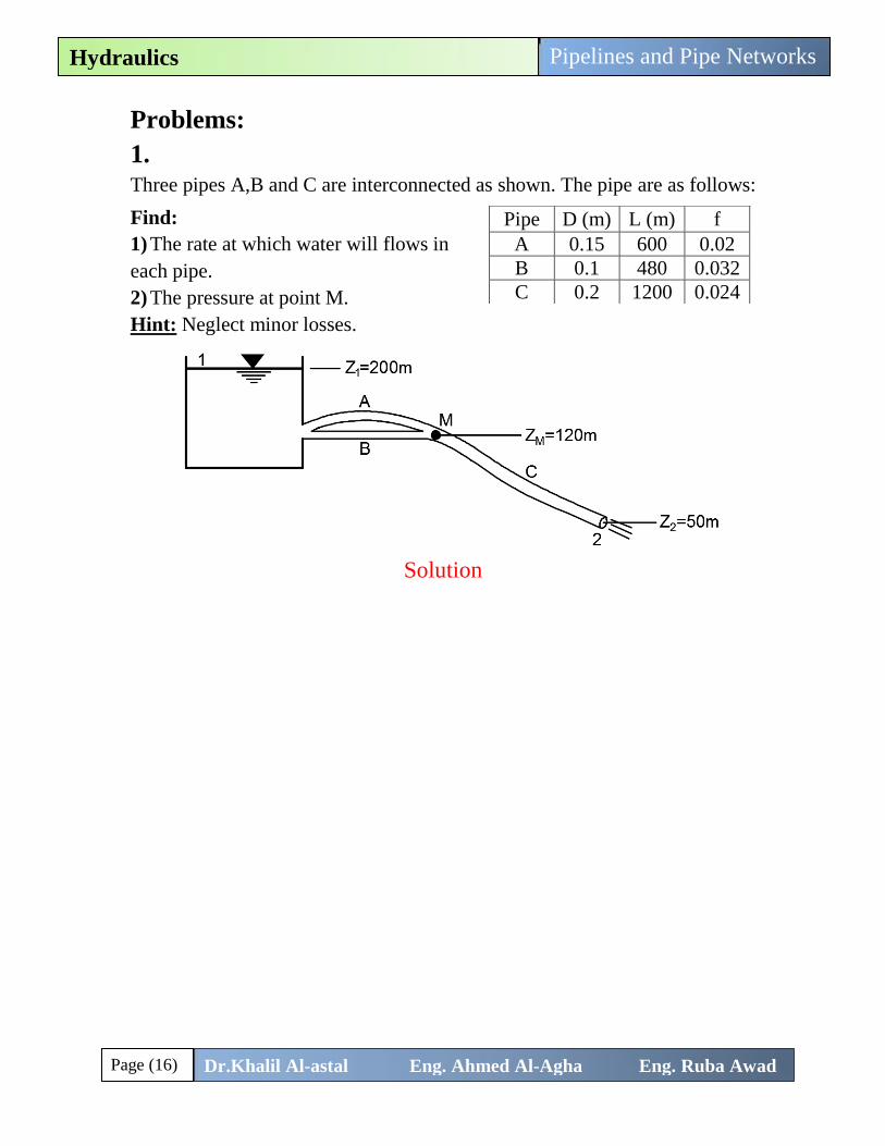
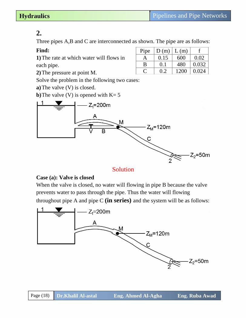
1. Three pipes A,B and C are interconnected as shown. The pipe are as follows:
Find:
1) The rate at which water will flows in
each pipe.
2) The pressure at point M.
Hint: Neglect minor losses.
Solution
Applying Bernoulli’s equation between the points 1 and 2.
P1
ρg+
V12
2g+ z1 =
P2
ρg+
V22
2g+ z2 + ∑ hL
P1 = V1 = P2 = 0.0 , V1 = VC =? ? , ∑ hL =? ?
0 + 0 + 200 = 0 +VC
2
19.62+ 50 + ∑ hL
0.0509 VC2 + ∑ hL = 150m → Eq. (1)
hf = f (L
D) (
V2
2g)
hf,A = hf,B (Parallel Pipes) (take pipe A)
∑ hL = hf,A + hf,C
hf,A = 0.02 (600
0.15) (
VA2
2g) = 4.07VA
2
Pipe D (m) L (m) f
A 0.15 600 0.02
B 0.1 480 0.032
C 0.2 1200 0.024
Page (17) Dr.Khalil Al-astal Eng. Ahmed Al-Agha Eng. Ruba Awad
Pipelines and Pipe Networks
Hydraulics
hf,C = 0.024 (1200
0.2) (
VC2
2g) = 7.34VC
2
∑ hL = 4.07VA2 + 7.34VC
2 (substitute in Eq. (1)) →
0.0509 VC2 + 4.07VA
2 + 7.34VC2 = 150m
→ 7.39VC2 + 4.07VA
2 = 150m → Eq. (2)
How we can find other relation between VA and VC? ?
Continuity Equation
QA + QB = QC π
4× 0.152VA +
π
4× 0.12VB =
π
4× 0.22VC
→ 0.025VA + 0.01VB = 0.04VC → Eq. (3)
But, hf,A = hf,B →
hf,A = 4.07VA2 (calculated above)
hf,B = 0.032 (480
0.1) (
VB2
2g) = 7.82VB
2
4.07VA2 = 7.82VB
2 → VB2 = 0.52 VA
2
→ VB = 0.72 VA (substitute in Eq. (3))
→ 0.025VA + 0.01(0.72 VA) = 0.04VC → VC = 0.805 VA (Subs. in Eq. 2)
→ 7.39(0.805 VA)2 + 4.07VA2 = 150m → VA = 4.11 m/s
→ VB = 0.72 × 4.11 = 2.13 m/s
→ VC = 0.805 × 4.11 = 3.3 m/s
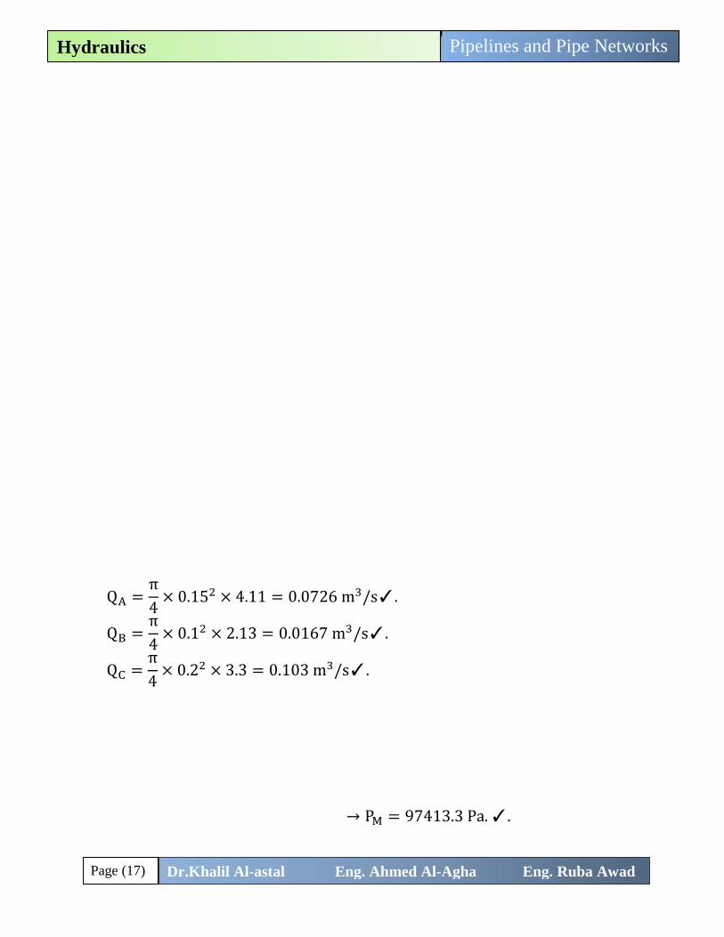
QA =π
4× 0.152 × 4.11 = 0.0726 m3/s✓.
QB =π
4× 0.12 × 2.13 = 0.0167 m3/s✓.
QC =π
4× 0.22 × 3.3 = 0.103 m3/s✓.
Pressure at M: → Bernoulli’s equation between the points M and 2.
PM
ρg+
VM2
2g+ zM =
P2
ρg+
V22
2g+ z2 + ∑ hL(M→2) VM = V2
∑ hL(M→2) = hf,C = 7.34 × 3.32 = 79.93m
→PM
9810+ 120 = 0 + 50 + 79.93 → PM = 97413.3 Pa.✓.
Page (18) Dr.Khalil Al-astal Eng. Ahmed Al-Agha Eng. Ruba Awad
Pipelines and Pipe Networks
Hydraulics
2. Three pipes A,B and C are interconnected as shown. The pipe are as follows:
Find:
1) The rate at which water will flows in
each pipe.
2) The pressure at point M.
Solve the problem in the following two cases:
a) The valve (V) is closed.
b) The valve (V) is opened with K= 5
Solution
Case (a): Valve is closed
When the valve is closed, no water will flowing in pipe B because the valve
prevents water to pass through the pipe. Thus the water will flowing
throughout pipe A and pipe C (in series) and the system will be as follows:
Pipe D (m) L (m) f
A 0.15 600 0.02
B 0.1 480 0.032
C 0.2 1200 0.024
Page (19) Dr.Khalil Al-astal Eng. Ahmed Al-Agha Eng. Ruba Awad
Pipelines and Pipe Networks
Hydraulics
Now, you can solve the problem as any problem (Pipes in series).
And if you are given the losses of the enlargement take it, if not, neglect it.
Case (b): Valve is Open
Here the solution procedures will be exactly the same as problem (1) >>
water will flow through pipe A and B and C, and pipes A and B are parallel
to each other .
But the only difference with problem (1) is:
Total head loss in pipe A = Total head loss in pipe B
Total head loss in pipe A = hf,A
Total head loss in pipe B = hf,B + hm,valve
hm,valve = KValve
VB2
2g= 5
VB2
2g
Now, we can complete the problem, as problem 1.
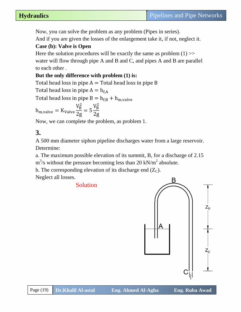
3. A 500 mm diameter siphon pipeline discharges water from a large reservoir.
Determine:
a. The maximum possible elevation of its summit, B, for a discharge of 2.15
m3/s without the pressure becoming less than 20 kN/m
2 absolute.
b. The corresponding elevation of its discharge end (ZC).
Neglect all losses.
Solution
Pabs = Patm + Pgauge
Pabs,B =20 × 103
9810= 2.038 m
Patm = 10.3m
Pgauge,B = 2.038 − 10.3 = −8.26m
Q = AV → V =Q
A=
2.15π4
× 0.52= 10.95 m/s
Applying Bernoulli’s equation between the
points A and B.
PA
ρg+
VA2
2g+ zA =
PB
ρg+
VB2
2g+ zB + ∑ hL
(Datum at A) , hL = 0 (given)
Page (20) Dr.Khalil Al-astal Eng. Ahmed Al-Agha Eng. Ruba Awad
Pipelines and Pipe Networks
Hydraulics
0 + 0 + 0 = −8.26 +10.952
19.62+ zB + 0 → zB = 2.15 m ✓.
Calculation of ZC:
Applying Bernoulli’s equation between the points A and C.
PA
ρg+
VA2
2g+ zA =
PC
ρg+
VC2
2g+ zC + ∑ hL
(Datum at A) , hL = 0 (given)
0 + 0 + 0 = 0 +10.952
19.62+ (−zC) → zC = 6.11 m ✓.
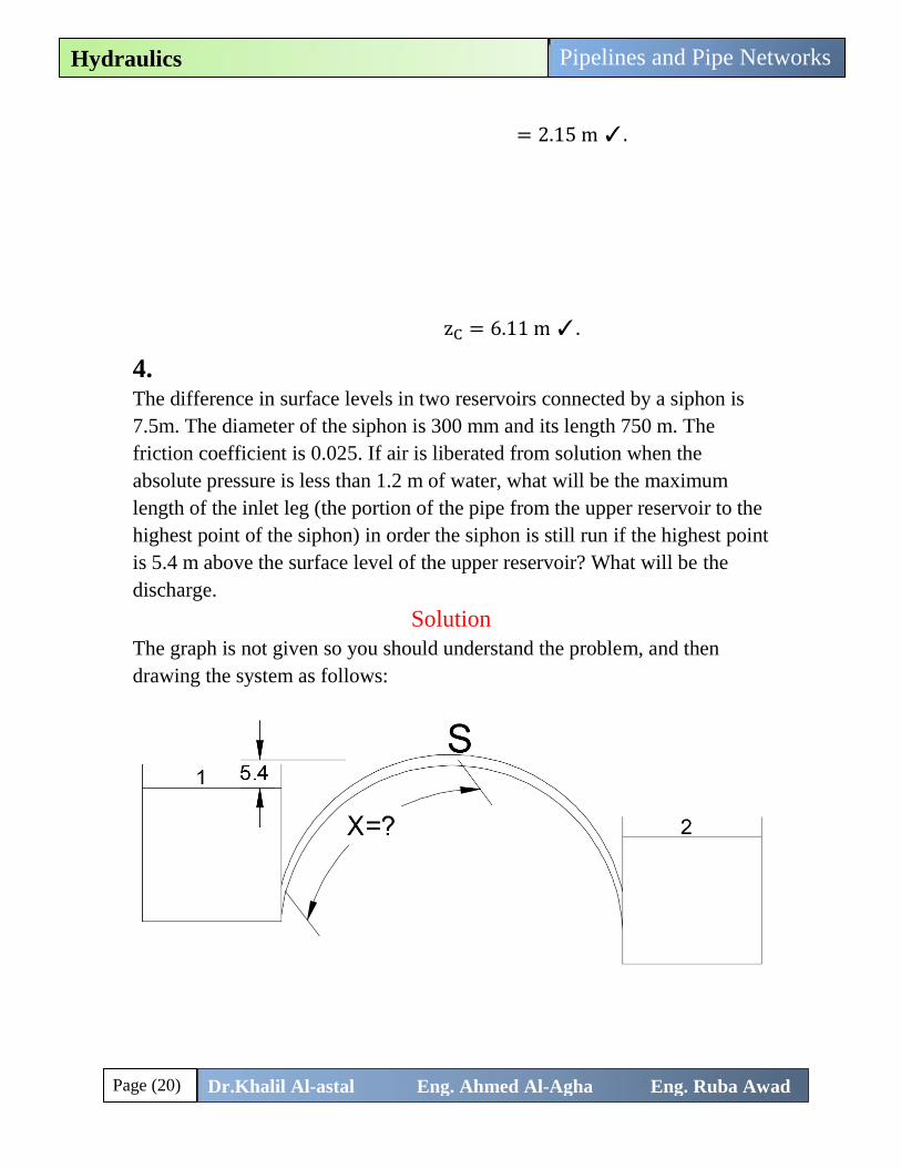
4. The difference in surface levels in two reservoirs connected by a siphon is
7.5m. The diameter of the siphon is 300 mm and its length 750 m. The
friction coefficient is 0.025. If air is liberated from solution when the
absolute pressure is less than 1.2 m of water, what will be the maximum
length of the inlet leg (the portion of the pipe from the upper reservoir to the
highest point of the siphon) in order the siphon is still run if the highest point
is 5.4 m above the surface level of the upper reservoir? What will be the
discharge.
Solution
The graph is not given so you should understand the problem, and then
drawing the system as follows:
Pabs = Patm + Pgauge
Pabs,S = 1.2m , Patm = 10.3m → Pgauge,S = 1.2 − 10.3 = −9.1m

Page (21) Dr.Khalil Al-astal Eng. Ahmed Al-Agha Eng. Ruba Awad
Pipelines and Pipe Networks
Hydraulics
Applying Bernoulli’s equation between the points 1 and S.
Datum at (1):
P1
ρg+
V12
2g+ z1 =
PS
ρg+
VS2
2g+ zS + ∑ hL(1→S)
0 + 0 + 0 = −9.1 +VS
2
2g+ 5.4 + ∑ hL(1→S) → Eq. (1)
∑ hL(1→S) = hf(1→S) = 0.025 (X
0.3) (
V2
19.62) But V =? ?
Applying Bernoulli’s equation between the points 1 and 2.
Datum at (2):
P1
ρg+
V12
2g+ z1 =
P2
ρg+
V22
2g+ z2 + ∑ hL(1→2)
0 + 0 + 7.5 = 0 + 0 + 0 + ∑ hL(1→2) → ∑ hL(1→2) = 7.5m
∑ hL(1→2) = 7.5m = hf(1→2) = 0.025 (750
0.3) (
V2
19.62) → V = 1.534m
hf(1→S) = 0.025 (X
0.3) (
1.5342
19.62) = 0.01X (Substitute in Eq. (1))
0 + 0 + 0 = −9.1 +VS
2
2g+ 5.4 + 0.01X (VS = V = 1.534)
0 + 0 + 0 = −9.1 +1.5342
2g+ 5.4 + 0.01X → X = 358m✓.
Page (22) Dr.Khalil Al-astal Eng. Ahmed Al-Agha Eng. Ruba Awad
Pipelines and Pipe Networks
Hydraulics
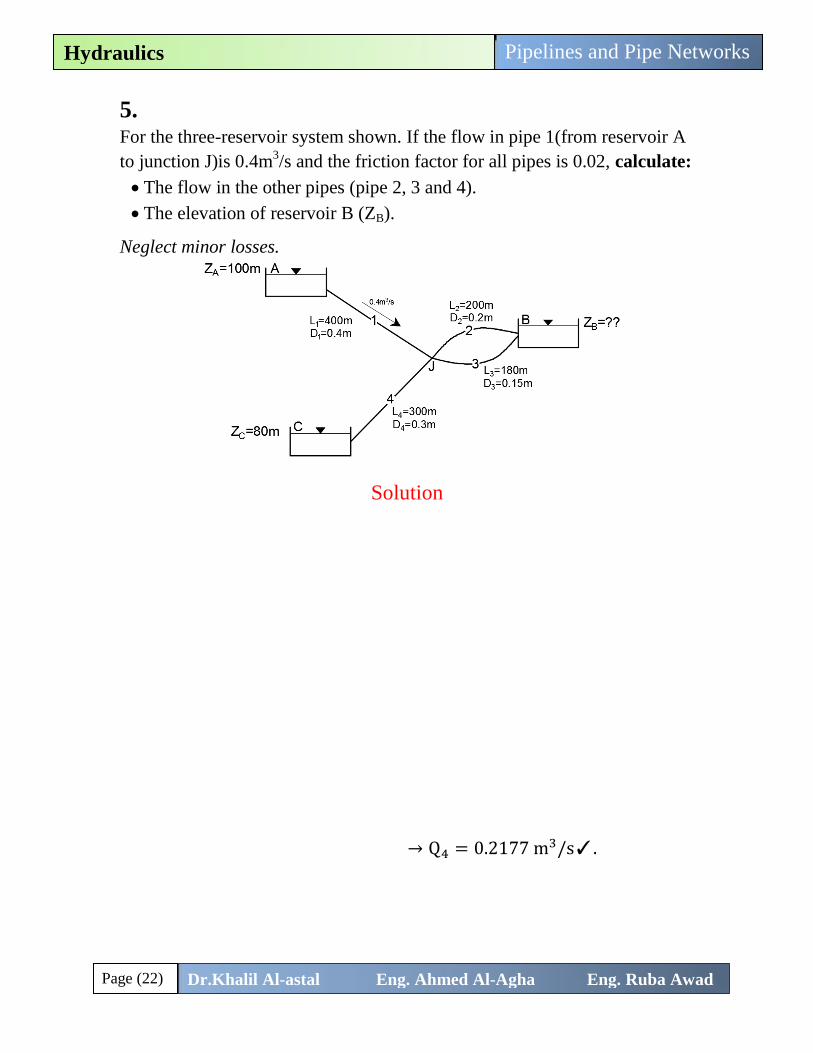
5. For the three-reservoir system shown. If the flow in pipe 1(from reservoir A
to junction J)is 0.4m3/s and the friction factor for all pipes is 0.02, calculate:
The flow in the other pipes (pipe 2, 3 and 4).
The elevation of reservoir B (ZB).
Neglect minor losses.
Solution
If we put a piezometer at point J, the will rise at height of Zp, which can be
calculated by applying Bernoulli’s equation between A and J:
PA
ρg+
VA2
2g+ zA =
PJ
ρg+
VJ2
2g+ ZP + ∑ hL(A→J)
0 + 0 + 100 = 0 + 0 + ZP + ∑ hL(A→J)
∑ hL(A→J) =8fLQ2
π2gD5=
8 × 0.02 × 400 × 0.42
π2g × 0.45= 10.32m
→ 100 − 10.32 = ZP = 89.68 m
Note that ZP = 89.68 > ZC = 80, So the flow direction is from J to C, and
to calculate this flow we apply Bernoulli’s equation between J and C:
ZP − ZC = ∑ hL(J→C)
89.68 − 80 =8 × 0.02 × 300 × Q4
2
π2g × 0.35→ Q4 = 0.2177 m3/s✓.
Now, by applying continuity equation at Junction J:
∑ Q@J = 0.0 → 0.4 = 0.2177 + ( Q2 + Q3) → Q2 + Q3 = 0.1823 m3/s
Page (23) Dr.Khalil Al-astal Eng. Ahmed Al-Agha Eng. Ruba Awad
Pipelines and Pipe Networks
Hydraulics
Since pipe 2 and 3 are in parallel, the head loss in these two pipes is the
same:
hL,2 = hL,3 →8fL2Q2
2
π2gD25 =
8fL3Q32
π2gD35
→8 × 0.02 × 200 × Q2
2
π2g × 0.25=
8 × 0.02 × 180 × Q32
π2g × 0.155→ Q3 = 0.513Q2
But, Q2 + Q3 = 0.1823 → Q2 + 0.513Q2 = 0.1823 → Q2 = 0.12 m3/s✓.
Q3 = 0.513 × 0.12 = 0.0618 m3/s✓.
Now we want to calculate the elevation ZB:
Apply Bernoulli’s equation between J and B:
ZP − ZB = ∑ hL(J→B) (take pipe 2)
89.68 − ZB =8 × 0.02 × 200 × 0.122
π2g × 0.25→ ZB = 74.8 m✓.
Page (24) Dr.Khalil Al-astal Eng. Ahmed Al-Agha Eng. Ruba Awad
Pipelines and Pipe Networks
Hydraulics
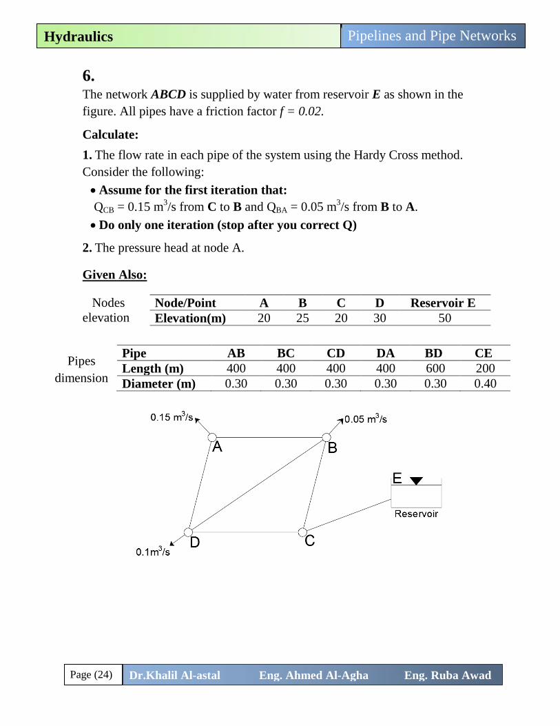
6. The network ABCD is supplied by water from reservoir E as shown in the
figure. All pipes have a friction factor f = 0.02.
Calculate:
1. The flow rate in each pipe of the system using the Hardy Cross method.
Consider the following:
Assume for the first iteration that:
QCB = 0.15 m3/s from C to B and QBA = 0.05 m
3/s from B to A.
Do only one iteration (stop after you correct Q)
2. The pressure head at node A.
Given Also:
Nodes
elevation
Node/Point A B C D Reservoir E
Elevation(m) 20 25 20 30 50
Pipe AB BC CD DA BD CE
Length (m) 400 400 400 400 600 200
Diameter (m) 0.30 0.30 0.30 0.30 0.30 0.40
Pipes
dimension
Page (25) Dr.Khalil Al-astal Eng. Ahmed Al-Agha Eng. Ruba Awad
Pipelines and Pipe Networks
Hydraulics
Solution
Firstly, from the given flows, we calculate the initial flow in each pipe and
the direction of flow through these pipes using continuity equation at each
note.
We calculate the corrected flow in each pipe, from the following tables:
Loop Pipe L D Qinitial hf
hf
Qinitial
∆ Qnew
I
AB 400 0.3 -0.05 -0.68 13.6 -0.025 -0.075
BD 600 0.3 +0.05 +1.02 20.4
DA 400 0.3 +0.1 +2.72 27.2 -0.025 +0.075
∑ +3.06 61.2
hf calculated for each pipe from the following relation:8fLQ2
π2gD5
∆=− ∑ hf
2 ∑hf
Qinitial
=−3.06
2 × 61.2= −0.025 m3/s
Qnew = Qinitial + ∆
Note that, we don’t correct pipe BD because is associated with the two
loops, so we calculate the flow in the associated pipe after calculating the
correction in each loop.
Always we assume
the direction of all
loops in clock wise
direction
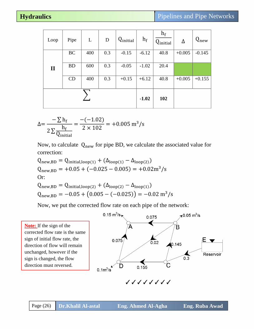
Page (26) Dr.Khalil Al-astal Eng. Ahmed Al-Agha Eng. Ruba Awad
Pipelines and Pipe Networks
Hydraulics
∆=− ∑ hf
2 ∑hf
Qinitial
=−(−1.02)
2 × 102= +0.005 m3/s
Now, to calculate Qnew for pipe BD, we calculate the associated value for
correction:
Qnew,BD = Qinitial,loop(1) + (∆loop(1) − ∆loop(2))
Qnew,BD = +0.05 + (−0.025 − 0.005) = +0.02m3/s
Or:
Qnew,BD = Qinitial,loop(2) + (∆loop(2) − ∆loop(1))
Qnew,BD = −0.05 + (0.005 − (−0.025)) = −0.02 m3/s
Now, we put the corrected flow rate on each pipe of the network:
✓✓✓✓✓✓✓✓
Loop Pipe L D Qinitial hf
hf
Qinitial
∆ Qnew
II
BC 400 0.3 -0.15 -6.12 40.8 +0.005 -0.145
BD 600 0.3 -0.05 -1.02 20.4
CD 400 0.3 +0.15 +6.12 40.8 +0.005 +0.155
∑ -1.02 102
Note: If the sign of the
corrected flow rate is the same
sign of initial flow rate, the
direction of flow will remain
unchanged, however if the
sign is changed, the flow
direction must reversed.
Page (27) Dr.Khalil Al-astal Eng. Ahmed Al-Agha Eng. Ruba Awad
Pipelines and Pipe Networks
Hydraulics
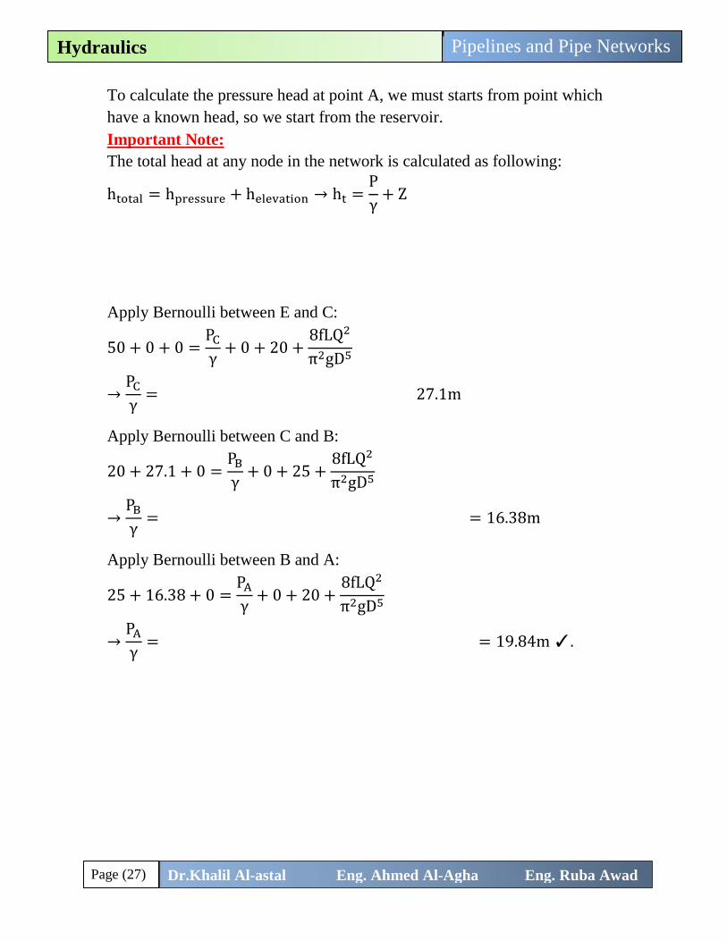
To calculate the pressure head at point A, we must starts from point which
have a known head, so we start from the reservoir.
Important Note:
The total head at any node in the network is calculated as following:
htotal = hpressure + helevation → ht =P
γ+ Z
By considering a piezometer at each node, such that the water rise on it
distance: P
γ+ Z and the velocity is zero.
Starts from reservoir at E:
Apply Bernoulli between E and C:
50 + 0 + 0 =PC
γ+ 0 + 20 +
8fLQ2
π2gD5
→PC
γ= 50 − 20 −
8 × 0.02 × 200 × 0.32
π2 × 9.81 × 0.45= 27.1m
Apply Bernoulli between C and B:
20 + 27.1 + 0 =PB
γ+ 0 + 25 +
8fLQ2
π2gD5
→PB
γ= 20 + 27.1 − 25 −
8 × 0.02 × 400 × 0.1452
π2 × 9.81 × 0.35= 16.38m
Apply Bernoulli between B and A:
25 + 16.38 + 0 =PA
γ+ 0 + 20 +
8fLQ2
π2gD5
→PA
γ= 25 + 16.38 − 20 −
8 × 0.02 × 400 × 0.0752
π2 × 9.81 × 0.35= 19.84m ✓.