View - SNO - Queen's University
69
PHYSICAL REVIEW C 75, 045502 (2007) Determination of the ν e and total 8 B solar neutrino fluxes using the Sudbury Neutrino Observatory Phase I data set B. Aharmim, 7 Q. R. Ahmad, 22 S. N. Ahmed, 17 R. C. Allen, 4 T. C. Andersen, 6 J. D. Anglin, 13 G. B¨ uhler, 4 J. C. Barton, 14,* E. W. Beier, 15 M. Bercovitch, 13 M. Bergevin, 6,8 J. Bigu, 7 S. D. Biller, 14 R. A. Black, 14 I. Blevis, 5 R. J. Boardman, 14 J. Boger, 3,† E. Bonvin, 17 M. G. Boulay, 10,17 M. G. Bowler, 14 T. J. Bowles, 10 S. J. Brice, 10,14,‡ M. C. Browne, 10,22 T. V. Bullard, 22 T. H. Burritt, 22 J. Cameron, 14 Y. D. Chan, 8 H. H. Chen, 4,* M. Chen, 17 X. Chen, 8,§ B. T. Cleveland, 14 J. H. M. Cowan, 7 D. F. Cowen, 15, G. A. Cox, 22 C. A. Currat, 8 X. Dai, 5,14,17 F. Dalnoki-Veress, 5,¶ W. F. Davidson, 13 H. Deng, 15 M. DiMarco, 17 P. J. Doe, 22 G. Doucas, 14 M. R. Dragowsky, 8,10,** C. A. Duba, 22 F. A. Duncan, 17,19 M. Dunford, 15,†† J. A. Dunmore, 14,‡‡ E. D. Earle, 17 S. R. Elliott, 10,22 H. C. Evans, 17 G. T. Ewan, 17 J. Farine, 7 H. Fergani, 14 A. P. Ferraris, 14 F. Fleurot, 7 R. J. Ford, 17,19 J. A. Formaggio, 12 M. M. Fowler, 10 K. Frame, 5,14 E. D. Frank, 15,§§ W. Frati, 15 N. Gagnon, 8,10,14,22 J. V. Germani, 10,22 S. Gil, 2, A. Goldschmidt, 10,¶¶ J. T. M. Goon, 11 K. Graham, 5 D. R. Grant, 5,** E. Guillian, 17 R. L. Hahn, 3 A. L. Hallin, 17 E. D. Hallman, 7 A. S. Hamer, 10,17,* A. A. Hamian, 22 W. B. Handler, 17 R. U. Haq, 7 C. K. Hargrove, 5 P. J. Harvey, 17 R. Hazama, 22,*** K. M. Heeger, 22,††† W. J. Heintzelman, 15 J. Heise, 2,10,17 R. L. Helmer, 21 R. Henning, 8 J. D. Hepburn, 17 H. Heron, 14 J. Hewett, 7 A. Hime, 10 C. Howard, 17 M. A. Howe, 22 M. Huang, 20 J. G. Hykaway, 7 M. C. P. Isaac, 8 P. Jagam, 6 B. Jamieson, 2 N. A. Jelley, 14 C. Jillings, 17 G. Jonkmans, 1,7 K. Kazkaz, 22 P. T. Keener, 15 K. Kirch, 10,‡‡‡ J. R. Klein, 20 A. B. Knox, 14 R. J. Komar, 2 L. L. Kormos, 17 M. Kos, 17 R. Kouzes, 16 A. Kr ¨ uger, 7 C. Kraus, 17 C. B. Krauss, 17 T. Kutter, 11 C. C. M. Kyba, 15 H. Labranche, 6 R. Lange, 3 J. Law, 6 I. T. Lawson, 6,19 M. Lay, 14 H. W. Lee, 17 K. T. Lesko, 8 J. R. Leslie, 17 I. Levine, 5,§§§ J. C. Loach, 14 W. Locke, 14 S. Luoma, 7 J. Lyon, 14 R. MacLellan, 17 S. Majerus, 14 H. B. Mak, 17 J. Maneira, 9 A. D. Marino, 8, R. Martin, 17 N. McCauley, 14,15,¶¶¶ A. B. McDonald, 17 D. S. McDonald, 15 K. McFarlane, 5 S. McGee, 22 G. McGregor, 14,‡ R. Meijer Drees, 22 H. Mes, 5 C. Mifflin, 5 K. K. S. Miknaitis, 22,†† M. L. Miller, 12 G. Milton, 1 B. A. Moffat, 17 B. Monreal, 12 M. Moorhead, 8,14 B. Morrissette, 19 C. W. Nally, 2 M. S. Neubauer, 15,**** F. M. Newcomer, 15 H. S. Ng, 2 B. G. Nickel, 6 A. J. Noble, 17 E. B. Norman, 8,†††† V. M. Novikov, 5 N. S. Oblath, 22 C. E. Okada, 8,‡‡‡‡ H. M. O’Keeffe, 14 R. W. Ollerhead, 6 M. Omori, 14 J. L. Orrell, 22,§§§§ S. M. Oser, 2 R. Ott, 12 S. J. M. Peeters, 14 A. W. P. Poon, 8 G. Prior, 8 S. D. Reitzner, 6 K. Rielage, 10,22 A. Roberge, 7 B. C. Robertson, 17 R. G. H. Robertson, 22 S. S. E. Rosendahl, 8, J. K. Rowley, 3 V. L. Rusu, 15,†† E. Saettler, 7 A. Sch¨ ulke, 8,¶¶¶¶ M. H. Schwendener, 7 J. A. Secrest, 15 H. Seifert, 7,10,22 M. Shatkay, 5 J. J. Simpson, 6 C. J. Sims, 14 D. Sinclair, 5,21 P. Skensved, 17 A. R. Smith, 8 M. W. E. Smith, 10,22 N. Starinsky, 5,8,10,22,***** T. D. Steiger, 22 R. G. Stokstad, 8 L. C. Stonehill, 10,22 R. S. Storey, 13,* B. Sur, 1,17 R. Tafirout, 7,††††† N. Tagg, 6,14,‡‡‡‡‡ Y. Takeuchi, 17 N. W. Tanner, 14 R. K. Taplin, 14 M. Thorman, 14 P. M. Thornewell, 10,14,22 N. Tolich, 8 P. T. Trent, 14 Y. I. Tserkovnyak, 2,§§§§§ T. Tsui, 2 C. D. Tunnell, 20 R. Van Berg, 15 R. G. Van de Water, 10,15 C. J. Virtue, 7 T. J. Walker, 12 B. L. Wall, 22 C. E. Waltham, 2 H. Wan Chan Tseung, 14 J.-X. Wang, 6 D. L. Wark, 18, J. Wendland, 2 N. West, 14 J. B. Wilhelmy, 10 J. F. Wilkerson, 22 J. R. Wilson, 14,¶¶¶¶¶ P. Wittich, 15,****** J. M. Wouters, 10 A. Wright, 17 M. Yeh, 3 and K. Zuber 14,¶¶¶¶¶ (SNO Collaboration) 1 Atomic Energy of Canada, Limited, Chalk River Laboratories, Chalk River, Ontario K0J 1J0, Canada 2 Department of Physics and Astronomy, University of British Columbia, Vancouver, British Columbia V6T 1Z1, Canada 3 Chemistry Department, Brookhaven National Laboratory, Upton, New York 11973-5000, USA 4 Department of Physics, University of California, Irvine, California 92717, USA 5 Ottawa-Carleton Institute for Physics, Department of Physics, Carleton University, Ottawa, Ontario K1S 5B6, Canada 6 Physics Department, University of Guelph, Guelph, Ontario N1G 2W1, Canada 7 Department of Physics and Astronomy, Laurentian University, Sudbury, Ontario P3E 2C6, Canada 8 Institute for Nuclear and Particle Astrophysics and Nuclear Science Division, Lawrence Berkeley National Laboratory, Berkeley, California 94720, USA 9 Laborat´ orio de Instrumentac ¸˜ ao e F´ ısica Experimental de Part´ ıculas, Av. Elias Garcia 14, 1 ◦ , P-1000-149 Lisboa, Portugal 10 Los Alamos National Laboratory, Los Alamos, New Mexico 87545, USA 11 Department of Physics and Astronomy, Louisiana State University, Baton Rouge, Louisiana 70803, USA 12 Laboratory for Nuclear Science, Massachusetts Institute of Technology, Cambridge, Massachusetts 02139, USA 13 National Research Council of Canada, Ottawa, Ontario K1A 0R6, Canada 14 Department of Physics, University of Oxford, Denys Wilkinson Building, Keble Road, Oxford OX1 3RH, United Kingdom 15 Department of Physics and Astronomy, University of Pennsylvania, Philadelphia, Pennsylvania 19104-6396, USA 16 Department of Physics, Princeton University, Princeton, New Jersey 08544, USA 17 Department of Physics, Queen’s University, Kingston, Ontario K7L 3N6, Canada 18 Rutherford Appleton Laboratory, Chilton, Didcot OX11 0QX, United Kingdom 19 SNOLAB, Sudbury, Ontario P3Y 1M3, Canada 20 Department of Physics, University of Texas at Austin, Austin, Texas 78712-0264, USA 21 TRIUMF, 4004 Wesbrook Mall, Vancouver, British Columbia V6T 2A3, Canada 22 Center for Experimental Nuclear Physics and Astrophysics, and Department of Physics, University of Washington, Seattle, Washington 98195, USA (Received 13 October 2006; published 27 April 2007) 0556-2813/2007/75(4)/045502(69) 045502-1 ©2007 The American Physical Society
Transcript of View - SNO - Queen's University
PHYSICAL REVIEW C 75, 045502 (2007)
Determination of the νe and total 8B solar neutrino fluxes using the Sudbury Neutrino ObservatoryPhase I data set
B. Aharmim,7 Q. R. Ahmad,22 S. N. Ahmed,17 R. C. Allen,4 T. C. Andersen,6 J. D. Anglin,13 G. Buhler,4 J. C. Barton,14,*
E. W. Beier,15 M. Bercovitch,13 M. Bergevin,6,8 J. Bigu,7 S. D. Biller,14 R. A. Black,14 I. Blevis,5 R. J. Boardman,14 J. Boger,3,†
E. Bonvin,17 M. G. Boulay,10,17 M. G. Bowler,14 T. J. Bowles,10 S. J. Brice,10,14,‡ M. C. Browne,10,22 T. V. Bullard,22
T. H. Burritt,22 J. Cameron,14 Y. D. Chan,8 H. H. Chen,4,* M. Chen,17 X. Chen,8,§ B. T. Cleveland,14 J. H. M. Cowan,7
D. F. Cowen,15,‖ G. A. Cox,22 C. A. Currat,8 X. Dai,5,14,17 F. Dalnoki-Veress,5,¶ W. F. Davidson,13 H. Deng,15 M. DiMarco,17
P. J. Doe,22 G. Doucas,14 M. R. Dragowsky,8,10,** C. A. Duba,22 F. A. Duncan,17,19 M. Dunford,15,†† J. A. Dunmore,14,‡‡
E. D. Earle,17 S. R. Elliott,10,22 H. C. Evans,17 G. T. Ewan,17 J. Farine,7 H. Fergani,14 A. P. Ferraris,14 F. Fleurot,7 R. J. Ford,17,19
J. A. Formaggio,12 M. M. Fowler,10 K. Frame,5,14 E. D. Frank,15,§§ W. Frati,15 N. Gagnon,8,10,14,22 J. V. Germani,10,22 S. Gil,2,‖‖A. Goldschmidt,10,¶¶ J. T. M. Goon,11 K. Graham,5 D. R. Grant,5,** E. Guillian,17 R. L. Hahn,3 A. L. Hallin,17 E. D. Hallman,7
A. S. Hamer,10,17,* A. A. Hamian,22 W. B. Handler,17 R. U. Haq,7 C. K. Hargrove,5 P. J. Harvey,17 R. Hazama,22,***
K. M. Heeger,22,††† W. J. Heintzelman,15 J. Heise,2,10,17 R. L. Helmer,21 R. Henning,8 J. D. Hepburn,17 H. Heron,14 J. Hewett,7
A. Hime,10 C. Howard,17 M. A. Howe,22 M. Huang,20 J. G. Hykaway,7 M. C. P. Isaac,8 P. Jagam,6 B. Jamieson,2 N. A. Jelley,14
C. Jillings,17 G. Jonkmans,1,7 K. Kazkaz,22 P. T. Keener,15 K. Kirch,10,‡‡‡ J. R. Klein,20 A. B. Knox,14 R. J. Komar,2
L. L. Kormos,17 M. Kos,17 R. Kouzes,16 A. Kruger,7 C. Kraus,17 C. B. Krauss,17 T. Kutter,11 C. C. M. Kyba,15 H. Labranche,6
R. Lange,3 J. Law,6 I. T. Lawson,6,19 M. Lay,14 H. W. Lee,17 K. T. Lesko,8 J. R. Leslie,17 I. Levine,5,§§§ J. C. Loach,14
W. Locke,14 S. Luoma,7 J. Lyon,14 R. MacLellan,17 S. Majerus,14 H. B. Mak,17 J. Maneira,9 A. D. Marino,8,‖‖‖ R. Martin,17
N. McCauley,14,15,¶¶¶ A. B. McDonald,17 D. S. McDonald,15 K. McFarlane,5 S. McGee,22 G. McGregor,14,‡ R. Meijer Drees,22
H. Mes,5 C. Mifflin,5 K. K. S. Miknaitis,22,†† M. L. Miller,12 G. Milton,1 B. A. Moffat,17 B. Monreal,12 M. Moorhead,8,14
B. Morrissette,19 C. W. Nally,2 M. S. Neubauer,15,**** F. M. Newcomer,15 H. S. Ng,2 B. G. Nickel,6 A. J. Noble,17
E. B. Norman,8,†††† V. M. Novikov,5 N. S. Oblath,22 C. E. Okada,8,‡‡‡‡ H. M. O’Keeffe,14 R. W. Ollerhead,6 M. Omori,14
J. L. Orrell,22,§§§§ S. M. Oser,2 R. Ott,12 S. J. M. Peeters,14 A. W. P. Poon,8 G. Prior,8 S. D. Reitzner,6 K. Rielage,10,22
A. Roberge,7 B. C. Robertson,17 R. G. H. Robertson,22 S. S. E. Rosendahl,8,‖‖‖‖ J. K. Rowley,3 V. L. Rusu,15,†† E. Saettler,7
A. Schulke,8,¶¶¶¶ M. H. Schwendener,7 J. A. Secrest,15 H. Seifert,7,10,22 M. Shatkay,5 J. J. Simpson,6 C. J. Sims,14
D. Sinclair,5,21 P. Skensved,17 A. R. Smith,8 M. W. E. Smith,10,22 N. Starinsky,5,8,10,22,***** T. D. Steiger,22 R. G. Stokstad,8
L. C. Stonehill,10,22 R. S. Storey,13,* B. Sur,1,17 R. Tafirout,7,††††† N. Tagg,6,14,‡‡‡‡‡ Y. Takeuchi,17 N. W. Tanner,14 R. K. Taplin,14
M. Thorman,14 P. M. Thornewell,10,14,22 N. Tolich,8 P. T. Trent,14 Y. I. Tserkovnyak,2,§§§§§ T. Tsui,2 C. D. Tunnell,20
R. Van Berg,15 R. G. Van de Water,10,15 C. J. Virtue,7 T. J. Walker,12 B. L. Wall,22 C. E. Waltham,2 H. Wan Chan Tseung,14
J.-X. Wang,6 D. L. Wark,18,‖‖‖‖‖ J. Wendland,2 N. West,14 J. B. Wilhelmy,10 J. F. Wilkerson,22 J. R. Wilson,14,¶¶¶¶¶
P. Wittich,15,****** J. M. Wouters,10 A. Wright,17 M. Yeh,3 and K. Zuber14,¶¶¶¶¶
(SNO Collaboration)1Atomic Energy of Canada, Limited, Chalk River Laboratories, Chalk River, Ontario K0J 1J0, Canada
2Department of Physics and Astronomy, University of British Columbia, Vancouver, British Columbia V6T 1Z1, Canada3Chemistry Department, Brookhaven National Laboratory, Upton, New York 11973-5000, USA
4Department of Physics, University of California, Irvine, California 92717, USA5Ottawa-Carleton Institute for Physics, Department of Physics, Carleton University, Ottawa, Ontario K1S 5B6, Canada
6Physics Department, University of Guelph, Guelph, Ontario N1G 2W1, Canada7Department of Physics and Astronomy, Laurentian University, Sudbury, Ontario P3E 2C6, Canada
8Institute for Nuclear and Particle Astrophysics and Nuclear Science Division, Lawrence Berkeley National Laboratory,Berkeley, California 94720, USA
9Laboratorio de Instrumentacao e Fısica Experimental de Partıculas, Av. Elias Garcia 14, 1◦, P-1000-149 Lisboa, Portugal
10Los Alamos National Laboratory, Los Alamos, New Mexico 87545, USA11Department of Physics and Astronomy, Louisiana State University, Baton Rouge, Louisiana 70803, USA
12Laboratory for Nuclear Science, Massachusetts Institute of Technology, Cambridge, Massachusetts 02139, USA13National Research Council of Canada, Ottawa, Ontario K1A 0R6, Canada
14Department of Physics, University of Oxford, Denys Wilkinson Building, Keble Road, Oxford OX1 3RH, United Kingdom15Department of Physics and Astronomy, University of Pennsylvania, Philadelphia, Pennsylvania 19104-6396, USA
16Department of Physics, Princeton University, Princeton, New Jersey 08544, USA17Department of Physics, Queen’s University, Kingston, Ontario K7L 3N6, Canada
18Rutherford Appleton Laboratory, Chilton, Didcot OX11 0QX, United Kingdom19SNOLAB, Sudbury, Ontario P3Y 1M3, Canada
20Department of Physics, University of Texas at Austin, Austin, Texas 78712-0264, USA21TRIUMF, 4004 Wesbrook Mall, Vancouver, British Columbia V6T 2A3, Canada
22Center for Experimental Nuclear Physics and Astrophysics, and Department of Physics, University of Washington,Seattle, Washington 98195, USA
(Received 13 October 2006; published 27 April 2007)
0556-2813/2007/75(4)/045502(69) 045502-1 ©2007 The American Physical Society
B. AHARMIM et al. PHYSICAL REVIEW C 75, 045502 (2007)
This article provides the complete description of results from the Phase I data set of the SudburyNeutrino Observatory (SNO). The Phase I data set is based on a 0.65 kiloton-year exposure of 2H2O(in the following denoted as D2O) to the solar 8B neutrino flux. Included here are details of the SNOphysics and detector model, evaluations of systematic uncertainties, and estimates of backgrounds. Alsodiscussed are SNO’s approach to statistical extraction of the signals from the three neutrino reactions (chargedcurrent, neutral current, and elastic scattering) and the results of a search for a day-night asymmetry inthe νe flux. Under the assumption that the 8B spectrum is undistorted, the measurements from this phaseyield a solar νe flux of φ(νe) = 1.76+0.05
−0.05 (stat.)+0.09−0.09 (syst.) × 106 cm−2 s−1 and a non-νe component of
φ(νµτ ) = 3.41+0.45−0.45 (stat.)+0.48
−0.45 (syst.) × 106 cm−2 s−1. The sum of these components provides a total flux inexcellent agreement with the predictions of standard solar models. The day-night asymmetry in the νe flux isfound to be Ae = 7.0 ± 4.9 (stat.)+1.3
−1.2% (syst.), when the asymmetry in the total flux is constrained to be zero.
DOI: 10.1103/PhysRevC.75.045502 PACS number(s): 26.65.+t, 14.60.Pq, 13.15.+g, 95.85.Ry
*Deceased.†Present address: U.S. Department of Energy, Germantown,
Maryland, USA.‡Present address: Fermilab, Batavia, Illinois, USA.§Present address: Goldman Sachs, 85 Broad Street, New York, USA.‖Present address: Department of Physics, Pennsylvania State Uni-
versity, University Park, Pennsylvania, USA.¶Present address: Department of Physics, Princeton University,
Princeton, New Jersey 08544, USA.**Present address: Department of Physics, Case Western Reserve
University, Cleveland, Ohio, USA.††Present address: Department of Physics, University of Chicago,
Chicago, Illinois, USA.‡‡Present address: Department of Physics, University of California,
Irvine, California, USA.§§Present address: Deparment of Mathematics and Computer Sci-
ence, Argonne National Laboratory, Lemont, Illinois, USA.‖‖Present address: University of Buenos Aires, Argentina.¶¶Present address: Lawrence Berkeley National Laboratory,
Berkeley, California, USA.***Present address: Department of Physics, Hiroshima University,
Hiroshima, Japan.†††Present address: Department of Physics, University of Wisconsin,
Madison, Wisconsin, USA.‡‡‡Present address: Paul Schiffer Institute, Villigen, Switzerland.§§§Present address: Department of Physics and Astronomy, Indiana
University, South Bend, Indiana, USA.‖‖‖Present address: Department of Physics, University of Toronto,
Toronto, Ontario, Canada.¶¶¶Present address: Department of Physics, University of
Liverpool, Liverpool, United Kingdom.****Present address: Department of Physics, University of California
at San Diego, La Jolla, California, USA.††††Present address: Lawrence Livermore National Laboratory,
Livermore, California, USA.‡‡‡‡Present address: Remote Sensing Lab, Post Office Box 98521,
Las Vegas, Nevada 89193, USA.§§§§Present address: Pacific Northwest National Laboratory,
Richland, Washington, USA.‖‖‖‖Present address: Department of Physics, Lund University, Lund,
Sweden.¶¶¶¶Present address: NEC Europe, Ltd., Kurfursten-Anlage 36,
D-69115 Heidelberg, Germany.*****Present address: Rene J.A. Levesque Laboratory, Universite de
Montreal, Montreal, Quebec, Canada.
I. INTRODUCTION
More than thirty years of solar neutrino experiments [1–6]indicated that the total flux of neutrinos from the Sun wassignificantly smaller than predicted by models of the Sun’senergy-generating mechanisms [7,8]. The deficit was not onlyuniversally observed but had an energy dependence that wasdifficult to attribute to astrophysical sources. The data wereconsistent with a negligible flux of neutrinos from solar7Be [9,10], though neutrinos from 8B (a product of solar7Be reactions) were observed. A natural explanation for theobservations was that neutrinos born as νes change flavor ontheir way to the Earth, thus producing an apparent deficit inexperiments detecting primarily νes. Neutrino oscillations—either in vacuum [11,12] or matter [13,14]—provide a mech-anism both for the flavor change and the observed energyvariations.
While these deficits argued strongly for neutrino flavorchange through oscillation, it was clear that a far more com-pelling demonstration would not resort to model predictionsbut look directly for neutrino flavors other than the νe emittedby the Sun. The Sudbury Neutrino Observatory (SNO) wasdesigned to do just that: provide direct evidence of solarneutrino flavor change through observation of non-electron-neutrino flavors by making a flavor-independent measurementof the total 8B neutrino flux from the Sun [15]. As a real-time detector, SNO was also designed to look for specificsignatures of the oscillation mechanism, such as energy- ortime-dependent survival probabilities. For example, dependingupon the values of the mixing parameters, the matter (MSW)effect leads to different νe fluxes during the day and the nightand to a distortion in the expected energy spectrum of 8B solarneutrinos.
†††††Present address: TRIUMF, 4004 Wesbrook Mall, Vancouver,British Columbia V6T 2A3, Canada.
‡‡‡‡‡Present address: Department of Physics and Astronomy, TuftsUniversity, Medford, Massachusetts, USA.
§§§§§Present address: Department of Physics, Harvard University,Cambridge, Massachusetts, USA.
‖‖‖‖‖Additional address: Imperial College, London SW7 2AZ, UnitedKingdom.
¶¶¶¶¶Present address: Department of Physics and Astronomy,University of Sussex, Brighton BN1 9QH, United Kingdom.
******Present address: Department of Physics, Cornell University,Ithaca, New York, USA.
045502-2
DETERMINATION OF THE νe AND . . . . I DATA SET PHYSICAL REVIEW C 75, 045502 (2007)
We present in this article the details of the analysespresented in previous SNO publications [16–18], including theexclusive νe and inclusive active neutrino fluxes, a measure-ment of the νe spectrum, the difference in the neutrino fluxesbetween day and night, and determination of the neutrinomixing parameters. We will concentrate here on the low-energythreshold measurements of Refs. [17,18], which included thefirst measurements of the total 8B flux, but will describe thedifferences between these analyses and the high-thresholdmeasurement presented in Ref. [16].
We begin in Sec. II with an overview of the SNO detectorand data analysis. In Sec. III we describe the data set used forthe measurements made in the initial phase (hereafter Phase I)of SNO using D2O without additives as the target-detector.Section IV describes the detector model ultimately used bothto calibrate the neutrino data and to provide distributionsused to fit our data. Section V describes the processingof the data, including all cuts applied, reconstruction ofposition and direction, and estimations of effective kineticenergy for each event. Section VI details the systematicuncertainties in the model, which translate into uncertaintiesin the neutrino fluxes. Section VII describes the measurementof backgrounds remaining in the data set, including neutronsfrom photodisintegration, the tails of low-energy radioactivity,and cosmogenic sources. Section VIII details the methods usedto fit for the neutrino rates, and Sec. IX the ingredients that gointo normalization of the rates. Sections X and XI present theflux results and results of a search for an asymmetry betweenthe day and night fluxes. Appendix A describes the methodsused to calculate mixing parameters from these data, andAppendix B gives details of the cuts we used to removeinstrumental backgrounds.
We will refer in this article to Ref. [16] as the “ES-CCpaper,” to Ref. [17] as the “NC paper,” and to Ref. [18]as the “Day-Night paper,” and collectively we call them the“Phase I publications.”
II. OVERVIEW OF SNO
A. The SNO detector
SNO is an imaging Cherenkov detector that uses heavywater (D2O) as both the interaction and detection medium [19].SNO is located in Inco’s Creighton Mine, at 46
◦28′30′′ N
latitude, 81◦12′04′′ W longitude. The detector resides 1730 m
below sea level with an overburden of 6020 m water equivalent,deep enough so that the rate of cosmic-ray muons passingthrough the entire active volume is just three per hour.
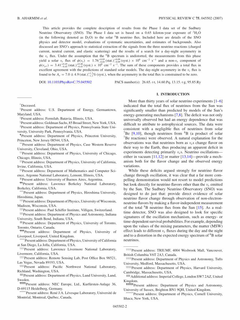
Figure 1 is a schematic of the detector. One thousandmetric tons of heavy water are contained in a 12-m-diametertransparent acrylic vessel (AV). Cherenkov light produced byneutrino interactions and radioactive backgrounds is detectedby an array of 9456 Hammamatsu model R1408 8-in.photomultiplier tubes (PMTs), supported by a stainless steelgeodesic sphere (the PMT support sphere or PSUP). EachPMT is surrounded by a light concentrator (“reflector”), whichincreases the photocathode coverage to nearly 55%. Thechannel discriminator thresholds are set to fire on 1/4 of aphotoelectron of charge. Over seven kilotons of light water
FIG. 1. (Color) Schematic of SNO detector.
shield the heavy water from external radioactive backgrounds:1.7 kT between the AV and the PMT support sphere, and5.7 kT between the PMT support sphere and the surroundingrock. The 5.7 kT of light water outside the PMT support sphereis viewed by 91 outward-facing 8-in. PMTs that are used foridentification of cosmic-ray muons. An additional 23 PMTs,arranged in a rectangular array, are suspended in the outerlight-water region. These 23 PMTs view the neck of the AV andare used primarily in the rejection of instrumentally generatedlight.
The detector is equipped with a versatile calibration deploy-ment system, which can place radioactive and optical sourcesover a large range of the x-z and y-z planes in the AV. Sourcesthat can be deployed include a diffuse multiwavelength laserfor measurements of PMT timing and optical parameters[20], a 16N source that provides a triggered sample of6.13-MeV γ rays [21], and a 8Li source that delivers tagged βswith an endpoint near 14 MeV [22]. In addition, high-energy(19.8 MeV) γ s are provided by a 3H(p, γ )4He (“pT”) source[23] and neutrons by a 252Cf source. Some of the sources canalso be deployed on vertical axes within the light-water volumebetween the AV and PMT support sphere.
B. Physics processes in SNO
SNO was designed to provide direct evidence of solarneutrino flavor change through comparisons of the interactionrates of three different processes:
νx + e− → νx + e− (ES),
νe + d → p + p + e− (CC),
νx + d → p + n + νx (NC).
045502-3
B. AHARMIM et al. PHYSICAL REVIEW C 75, 045502 (2007)
The first reaction, elastic scattering (ES) of electrons, hasbeen used to detect solar neutrinos in other water Cherenkovexperiments. It has the great advantage that the recoil electrondirection is strongly correlated with the direction of theincident neutrino, and hence the direction to the Sun (cos θ�).This ES reaction is sensitive to all neutrino flavors. For νes,the elastic scattering reaction has both charged and neutralcurrent components, making the cross section for νes ∼6.5 times larger than that for νµs or ντ s.
Deuterium in the heavy water provides loosely boundneutron targets for an exclusively charged current (CC)reaction, which, at solar neutrino energies, occurs only forνes. In addition to providing exclusive sensitivity to νes, thisreaction has the advantage that the recoil electron energy isstrongly correlated with the incident neutrino energy, and thusit can provide a precise measurement of the 8B neutrino energyspectrum. The CC reaction also has an angular correlationwith the Sun that falls as (1 − 0.340cos θ�) [24] and has across section roughly 10 times larger than the ES reaction forneutrinos within SNO’s energy acceptance window.
The third reaction, also unique to heavy water, is a purelyneutral current (NC) process. This has the advantage that itis equally sensitive to all neutrino flavors and thus providesa direct measurement of the total active flux of 8B neutrinosfrom the Sun. Like the CC reaction, the NC reaction has across section nearly 10 times as large as the ES reaction.
For both the ES and CC reactions, the recoil electrons aredetected directly through their production of Cherenkov light.For the NC reaction, the neutrons are not seen directly but aredetected in a multistep process. When a neutrino liberates aneutron from a deuteron, the neutron thermalizes in the D2Oand may eventually be captured by another deuteron, releasinga 6.25-MeV γ ray. The γ ray either Compton scatters anelectron or produces an e+e− pair, and the Cherenkov radiationof these secondaries is detected.
To determine whether neutrinos that start out as νes in thesolar core convert to another flavor before detection on Earth,we have two methods: comparison of the CC reaction rateto the NC reaction rate or comparison of the CC rate to theES rate. The NC-CC comparison has the advantage of highsensitivity. When we compare the total flux to the νe flux,we expect the former to be roughly three times the latter ifboth solar neutrino experiments and standard solar models arecorrect. In addition, many uncertainties in the cross sectionsfor the two processes will largely cancel.
The comparison of CC to ES has the advantage thatrecoil electrons from both reactions provide neutrino spec-tral information. The spectral information can ultimatelybe used to show that any excess in the ES reaction overthe CC reaction is not caused by a difference in the ef-fective neutrino energy thresholds used to analyze the tworeactions [25,26]. The CC-ES comparison also has theadvantage that the strong angular correlation of the ESelectrons with the direction to the Sun demonstrates thatany excess seen is not due to some unexpected nonsolarbackground. Lastly, the CC-ES comparison can be made byusing both SNO’s ES measurement and the high-precision ESmeasurement made by the Super-Kamiokande Collaboration[5]. This provides a high sensitivity cross-check for the
0
0.025
0.05
0.075
0.1
5 10 150
0.05
0.1
0.15
5 10 150
0.050.1
0.150.2
5 10 15
00.025
0.050.075
0.1
0 0.5 1 1.50
0.02
0.04
0.06
0 0.5 1 1.50
0.05
0.1
0.15
0 0.5 1 1.5
0
0.02
0.04
-1 0 10
0.2
0.4
-1 0 1
CC ES NC
T/MeV
Prob
abili
ty p
er b
in
(R/RAV)3
cosθo.
00.010.020.030.04
-1 0 1
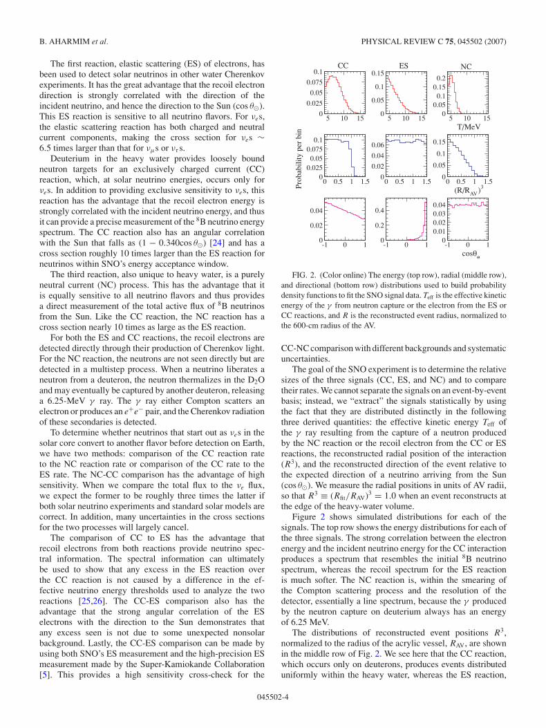
FIG. 2. (Color online) The energy (top row), radial (middle row),and directional (bottom row) distributions used to build probabilitydensity functions to fit the SNO signal data. Teff is the effective kineticenergy of the γ from neutron capture or the electron from the ES orCC reactions, and R is the reconstructed event radius, normalized tothe 600-cm radius of the AV.
CC-NC comparison with different backgrounds and systematicuncertainties.
The goal of the SNO experiment is to determine the relativesizes of the three signals (CC, ES, and NC) and to comparetheir rates. We cannot separate the signals on an event-by-eventbasis; instead, we “extract” the signals statistically by usingthe fact that they are distributed distinctly in the followingthree derived quantities: the effective kinetic energy Teff ofthe γ ray resulting from the capture of a neutron producedby the NC reaction or the recoil electron from the CC or ESreactions, the reconstructed radial position of the interaction(R3), and the reconstructed direction of the event relative tothe expected direction of a neutrino arriving from the Sun(cos θ�). We measure the radial positions in units of AV radii,so that R3 ≡ (Rfit/RAV)3 = 1.0 when an event reconstructs atthe edge of the heavy-water volume.
Figure 2 shows simulated distributions for each of thesignals. The top row shows the energy distributions for each ofthe three signals. The strong correlation between the electronenergy and the incident neutrino energy for the CC interactionproduces a spectrum that resembles the initial 8B neutrinospectrum, whereas the recoil spectrum for the ES reactionis much softer. The NC reaction is, within the smearing ofthe Compton scattering process and the resolution of thedetector, essentially a line spectrum, because the γ producedby the neutron capture on deuterium always has an energyof 6.25 MeV.
The distributions of reconstructed event positions R3,normalized to the radius of the acrylic vessel, RAV, are shownin the middle row of Fig. 2. We see here that the CC reaction,which occurs only on deuterons, produces events distributeduniformly within the heavy water, whereas the ES reaction,
045502-4
DETERMINATION OF THE νe AND . . . . I DATA SET PHYSICAL REVIEW C 75, 045502 (2007)
which can occur on any electron, produces events distributeduniformly well beyond the heavy-water volume. The smallleakage of events just outside the heavy-water volume (justoutside R3 = 1) for the CC reaction is due to the resolutiontail of the reconstruction algorithm.
The NC signal, however, does not have a uniform dis-tribution inside the heavy water, but instead it decreasesmonotonically from the central region to the edge of theAV. The reason for this is the long (∼ 120 cm) thermaldiffusion length for neutrons in D2O. Neutrons produced nearthe edge of the heavy-water volume have a high probability ofwandering outside it, at which point they can be capturedon hydrogen either in the AV or by the H2O surroundingthe vessel. The capture cross section on hydrogen is nearly600 times larger than on deuterium, and therefore thesehydrogen captures occur almost immediately, leaving noopportunity for the neutrons to diffuse back into the fiducialvolume. Further, such hydrogen captures produce a 2.2-MeVγ ray, which is well below the analysis threshold, and thereforeevents from these captures do not appear in the NC R3
distribution shown in Fig. 2.The bottom row of Fig. 2 shows the reconstructed direction
distribution of the events. In the middle of that row we see thepeaking of the ES reaction, pointing away from the Sun. The∼1 − 1/3cos θ� distribution of the CC reaction is also clearin the left-most plot. The NC reaction shows no correlationwith the solar direction—the γ ray from the captured neutroncarries no directional information about the incident neutrino.
One last point needs to be made regarding the distributionslabeled “NC” in Fig. 2: They represent equally well thedetector response to any neutrons, not just those producedby neutral current interactions, as long as the neutrons aredistributed uniformly in the detector. For example, neutronsproduced through photodisintegration by γ rays emitted byradioactivity inside the D2O will have the same distributionsof energy, radial position, and direction as those produced bysolar neutrinos. These neutrons are an irreducible backgroundin the data analysis and must be kept small through purificationof detector materials.
C. Analysis strategy
To determine the sizes of the CC, ES, and NC signalswe use the nine distributions of Fig. 2 to create probabilitydensity functions (pdfs) and perform a generalized maximumlikelihood fit of the data to the same distributions. There are,however, three principal prerequisites before we can begin this“signal-extraction” process: We must process the data so thatwe can create distributions of event energies, positions, anddirections; we need to build a model of the detector so that wecan create the pdfs like those in Fig. 2; and we need to providemeasurements of any residual backgrounds.
Data processing begins with the calibration of the raw data,converting analog-to-digital converter (ADC) values into PMTcharges and times. The calibrated charges and times allow usto reconstruct each event’s position and direction, as well asestimate event energy. We also apply cuts to the data set duringprocessing to remove as many background events as possiblewithout sacrificing a substantial number of neutrino signalevents.
In the signal-extraction process described here we implic-itly assume that the pdfs used in the fit are built from acomplete and accurate representation of the detector’s trueresponse. The model we use to create the pdfs must thereforedescribe everything from the physics of neutrino interactions,to the propagation of particles and optical photons through thedetector media, to the behavior of the data-acquisition system.The model needs to reproduce the response to signal eventsat all places in the detector, for all neutrino directions, for allneutrino energies, and for all times. It must also track changesin the detector over time, such as failed PMTs or electronicschannels.
Although our suite of cuts is very efficient at removingbackground events, we nevertheless must demonstrate thatthe residual background levels are negligible or we mustproduce measurements of their size. The latter is particularlyimportant for the photodisintegration neutrons—because theylook identical to the NC signal, they cannot be removed, andmust be measured and subtracted from the total neutron countresulting from the maximum likelihood fit.
Signal extraction estimates the numbers of CC, NC, and ESevents; conversion to fluxes requires acceptance correctionsfor each of the signals and, for the NC signal, adjustmentsfor the capture efficiency of neutrons on deuterons. The finalnormalization also includes neutrino interaction cross sections,detector live time, and the number of available targets.
For our Phase I publications we performed three indepen-dent analyses of the data presented in this article [27–29]. Priorto perfoming the final processing, we chose from these threeanalyses two independent approaches for each major analysiscomponent (cut sets, reconstruction algorithms, energy cali-bration, etc.). Comparisons of the results of the independentapproaches were used to validate every component of theanalysis—one approach was designated “primary” and usedfor the Phase I published results, and one was designated“secondary” and used as the verification check. (Table XXVIlists the approaches for each of the analysis components.)In this article, we describe both the primary and secondaryapproaches used.
III. DATA SET
The data set used in the analysis we describe here wasacquired between November 2, 1999, and May 31, 2001,and represents a total of 306.4 live days. Although the SNOdetector is live to neutrinos during nearly all calibrations,data taken during the calibration periods—roughly 10% ofthe time the detector is running—are not used for solarneutrino analysis. Other losses of live time result from minepower outages, detector maintenance periods, and the lossof underground laboratory communication or environmentalsystems.
The SNO data set is divided into “runs,” a new run beingstarted either at a change in detector conditions (such asthe insertion of a calibration source) or after a maximumduration has been exceeded (in Phase I, no more than fourdays). The runs used for the final analysis were selected basedupon criteria external to the data themselves. Selected runs
045502-5
B. AHARMIM et al. PHYSICAL REVIEW C 75, 045502 (2007)
were those for which calibration sources were not present inthe detector, no major electronics systems were off-line, nomaintenance was being performed, and no circulation of theD2O that caused light to be produced inside the detector wasbeing undertaken.
The SNO detector responds to several triggers, the primaryone being a coincidence of 18 or more PMTs firing within aperiod of ∼93 ns. (The threshold was lowered to 16 or morePMTs after December 20, 2000.) The rate of such triggersaveraged roughly 5 Hz. The detector also triggered if the totalcharge collected in all PMTs exceeded 150 photoelectrons. A“random” trigger pulsed the detector at 5 Hz throughout thedata set, and a prescaled trigger fired after every thousandth 11-PMT threshold crossing. Information about which conditioncaused the trigger for a given event was saved as part of theprimary data stream. The overall trigger rate was between 15and 20 Hz.
Although the overall detector configuration was kept stableduring the data-taking period, we performed two fixes worthyof comment. The first was a change to the charge- and time-digitizing ADCs. Soon after the start of production running, itwas discovered that the ADCs were developing nonlinearitieswell beyond their specification. During most of the data-takingperiod, bad ADCs were periodically replaced or repaired,but on August 18, 2000, a permanent fix was implemented.In addition, roughly halfway through the data-taking period,we discovered a small rate dependence to the PMT timingmeasurements. Although small, the rate dependence did affectour position reconstruction. We developed a hardware solutionto mitigate the effect and also created an off-line calibration toremove it. The hardware change was completed in December,2000, and the off-line calibration was applied to the entire dataset.
Other minor changes—failure of individual PMTs (at anaverage rate of about 1% per year), alteration of front-end discriminator thresholds, or repair of broken electronicschannels—were tracked and the status of every channel wasstored in the SNO database at the beginning of each run foruse in the off-line data analysis. In addition, the front-endelectronics timing and charge responses were calibrated twiceeach week, much more frequently than the observed variationsof pedestals or slopes. Calibration of phototube gain, timing,and rise-time response was done roughly monthly.
To provide a final check against statistical bias, the data setwas divided in two, an “open” data set, to which all analysisprocedures and methods were applied, and a “blind” data set,upon which no analysis within the signal region (between 40and 200 hit phototubes) was performed until the full analysisprogram had been finalized. The blind data set began at theend of June 2000, at which point we began analyzing just 10%of the data set, leaving the remaining 90% blind. The total sizeof the blind data set thus corresponded to roughly 30% of thetotal live time.
IV. PHYSICS AND DETECTOR MODEL
Both reconstruction of event kinetic energy and construc-tion of the distributions shown in Fig. 2 require a model of
the detector’s response to Cherenkov light created by neutrinointeractions. For energy reconstruction, the model we use forthe response is analytical, and for the creation of the pdfs inFig. 2 the model is a Monte Carlo simulation. Most of therequired inputs are the same for both models: the physicsof the passage of electrons and γ rays through the variousdetector media and the associated production of Cherenkovlight, the optical properties of the detector, and the state andresponse of the detector PMTs, electronics, and trigger. Inaddition, for the Monte Carlo simulation to correctly predictthe energy spectra and direction distributions, it must includethe total and differential cross sections for the CC, ES, andNC neutrino interactions, as well as the incident 8B neutrinospectrum. Lastly, to produce the correct radial distributionsfor the neutrons from the NC reaction, the Monte Carlomodel also simulates the transport and capture of low-energy(<20 MeV) neutrons.
In the following section, we describe the details of eachcomponent of the models and the calibrations applied. Aswill be seen here and in subsequent sections of this article, theMonte Carlo simulation reproduced nearly all the distributionsof interest we measured with our calibration sources to a highdegree of accuracy.
A. Neutrino spectrum and interactions
In the Monte Carlo model, neutrino energies are picked byweighting the 8B neutrino energy spectrum by the neutrinointeraction cross sections σ (Eν) for each of the three reactions(ES, CC, and NC). The energies and directions of thesecondary electrons and neutrons are generated through aconvolution of the 8B spectrum measured by Ortiz et al. [30]with the corresponding normalized double differential crosssections d2N/dEd�. For the ES reaction, the simulation usedthe cross sections as presented by Bahcall [31], which do notinclude radiative corrections (a roughly 2% correction thatwas later applied to the extracted ES rate—see Sec. X). Forthe CC and NC reactions we used the calculations by Butler,Chen, and Kong (BCK) [32], with an L1,A scale factor of5.6 fm3, but then rescaled the overall cross sections to thevalues found by Nakamura et al. [33] and applied correctionfactors to account for the radiative corrections as determinedby Kurylov et al. [34]. As a general verification check,we also ran the simulation with several other cross sectioncalculations [35,36], which show agreement at the 1–2% level.The simulation did not include variation in the fluxes owingto the eccentricity of the Earth’s orbit—this variation andits uncertainty were included at a later stage in the analysis(see Sec. X).
B. Background processes
Radioactive backgrounds are also modeled through MonteCarlo simulation. The simulation includes the branchingfractions into βs and γ s of each nuclide known to be presentin the detector, as well as angular correlations between decayγ rays if appropriate. The background events can be generatedwithin any of the media represented in the Monte Carlo
045502-6
DETERMINATION OF THE νe AND . . . . I DATA SET PHYSICAL REVIEW C 75, 045502 (2007)
simulation, including the D2O, H2O, acrylic, Vectran supportropes, PMT glass and related components, and the PMTsupport structure.
C. Cherenkov light from electrons and γ -ray interactions
The Monte Carlo simulation of the neutrino interactionsand backgrounds produces electrons and γ rays whose initialenergy and angular distributions depend only upon neutrinoand nuclear physics. We have compared the output of thesimulation at this stage to analytic calculations of thesedistributions and find excellent agreement.
To go from the initial energy and angular distributions tothe photons seen by the photomultiplier tubes, the MonteCarlo model simulates both the propagation and interactionof electrons, neutrons, and γ rays within the detector mediaand the consequent production of Cherenkov light.
We used the EGS4 [37] (electron gamma shower) code tosimulate the interactions of electrons and γ rays. EGS4 providessome critical pieces of physics: conversion of γ rays intoelectrons through Compton scattering, pair production, and thephotoelectric effect; and energy loss and multiple scattering ofelectrons [38]. At solar neutrino energies, multiple scatteringof the electrons as they propagate severely distorts theCherenkov cone, and we therefore simulate the productionof Cherenkov light by adding Cherenkov photons along eachelectron’s entire trajectory.
The EGS4 code simulates individual tracks by a series ofstraight segments, with a small fractional change in the kineticenergy in each step arising from energy loss in the medium. Atthe end of each step an angular deflection is generated, drawnfrom the Moliere distribution, to simulate multiple scattering.If all Cherenkov photons from a given step are produced atthe Cherenkov angle θc relative to the direction of the straighttrack segment, the final pattern will be a series of cones. Ifthe step size is doubled the number of cones is halved; theangular distribution of the Cherenkov light is thus sensitive tothe step size. This artifact is removed by linearly interpolating,for each photon generated, the local direction cosines of thetrack between successive steps.
To choose the optimal EGS4 step size, we compared theoutput of our implementation of the EGS4 code to dataon electron scattering; we found that energy step sizes inthe range of 0.001 to 0.05 MeV reproduced the data best[39]. We verified the EGS4 treatment of multiple scatteringby comparing output Cherenkov distributions averaged overmany electron trajectories with those from an independentGoudsmit-Sanderson treatment of multiple scattering. With astep size of 1% in energy loss, we found very good agreementwhen the interpolation of direction cosines is included, evenat energies as low as 1 MeV.
For generating Cherenkov light on each segment of anelectron’s path, we use the asymptotic formula for light yield:
dI
dω= ωe2Lsin2θc
c2. (1)
In Eq. (1), the yield I (with dimensions of energy per unitfrequency interval) is given as a function of angular frequency
ω and is proportional to path length L. We have verified theuse of this asymptotic formula by calculating the interferencebetween two unaligned segments and have found that theinterference does not produce significant lowering of lightyield.
The number of photons produced is then sampled from aPoisson distribution and the creation points of these photonsare positioned randomly along the segment. Photons areemitted at an angle θc to the electron track direction, whichis interpolated as just described, and is kept fixed within eachstep of the track.
D. Neutron transport
In addition to electrons and γ rays, the Monte Carlomodel must account for the propagation and capture ofneutrons throughout the detector media. The most importantof these neutrons are those that result from disintegration ofdeuterons through neutrino neutral current interactions andthose produced through photodisintegration of the deuteronsby γ rays.
For neutron propagation, we use the MCNP [40] neutrontransport code developed at Los Alamos National Laboratory,but we restrict its use to the propagation of neutrons, ignoringadditional particles (e.g., αs) that may be created by neutroninteractions. The creation of additional particles is recorded,but the particles are not propagated, with the exception ofγ rays and electrons, which are handled by EGS4. MCNP
was chosen because of its widespread verification and usage,and because of its sophisticated handling of thermal neutrontransport in general and molecular effects in H2O and D2Oin particular, without which accurate simulation of neutrontransport in the SNO detector could not be carried out.
MCNP is primarily intended as a nonanalog code, whichuses weighted sampling techniques to study rare processes. Ithas a set of physics-related routines that form the core of itssimulated neutron transport, and it is these that are used in theMonte Carlo simulation. The MCNP code uses extensive datatables to provide partial and total interaction cross sections asa function of neutron energy, the energy-angle spectrum of theemergent neutrons, and other interaction data.
To verify our implementation of MCNP, we compared manyof the low-level simulation parameters in several differentmedia, such as the neutron step length, the emitted neutronenergy, and the directions of initial and final trajectories foreach interaction. We performed these tests for neutron energiesfrom 10−3 eV to 10 MeV, and in over a thousand comparisonsof distributions between MCNP and our simulation, none werefound to be anomalous.
We also checked that our simulation could reproducerepresentative cross sections at thermal energies and matchthe diffusion equation closely in the limit � � �a , where� and �a are the macroscopic interaction and absorptioncross sections, respectively. MCNP (and hence our simulation)has been shown by Wang et al. [41] to predict the absolutenumber of neutrons captured in an experiment involvingneutron thermalization with an accuracy of at worst 3%. Atthe same time, Wang et al. have shown that the ratio of the
045502-7
B. AHARMIM et al. PHYSICAL REVIEW C 75, 045502 (2007)
numbers of captured neutrons predicted by MCNP in relatedexperimental setups is accurate to within 0.3%. Based on ourstudies, we believe these numbers apply to the SNO detectoras well.
E. High-energy processes
To simulate muon events and any other lepton above2 GeV, the SNO Monte Carlo simulation relies on the CERNpackage LEPTO 6.3 [42,43]. The lower energy electromagneticcomponents of the resultant muon showers are then passed tothe EGS4 code and the rest of the SNO simulation, as describedin the previous section. Hadrons produced by the interactionof these muons are handled by the FLUKA and GCALOR
packages.
F. Detector geometry
The Monte Carlo simulation includes a detailed model ofthe detector geometry, including the position and orientationof the PMT support sphere and its resident PMTs, the positionand thickness of the AV including support plates and ropes,the size and position of the AV “neck,” and a full modelof the structure of the PMTs and their associated lightconcentrators. The values were based primarily upon surveysand measurements taken before the elements were installedin the detector. The positions of the acrylic sphere and PMTsupport sphere were updated after the detector was filled withwater, to account for the effects of buoyancy. For the work wedescribe in this article, for all simulations it is assumed thatthe AV and PMT support sphere were concentric, though smalladjustments to this were made at a later stage in the analysis(see Sec. VIII).
The orientation of the PMT array with respect to true Northwas determined on the cavity deck after the detector wasconstructed and filled with water, by surveying chords betweenthe PMT array suspension points with a commercial marinegyrocompass. Multiple chords were surveyed and averagedand coupled to detailed deck surveys, PMT array constructiondrawings, and field tests of the geodesic sphere’s rigidity. Theabsolute orientation of the array was determined to 0.5◦. Thissurvey was in reasonable agreement (2.5◦) with the originalInco mine surveys. The coordinate system used for the MonteCarlo model and for data analysis put z along the detector’svertical axis and x along true North.
G. Detector and PMT optics
By far the most important parts of the detector modelare the optical properties of the detector media and thephotomultiplier tubes. SNO is optically more complex thanprevious water Cherenkov detectors: Photons traverse multipleoptical media from the fiducial volume to the PMTs, andthe light concentrators surrounding the PMTs have their ownoptical properties. Therefore the energy response of the SNOdetector varies significantly with radial position and eventdirection—an event near the edge of the volume and pointing
outward produces a very different number of hits (∼5%) thanan event pointing inward, which is yet different from an eventnear the center. For more detailed descriptions of the opticalmeasurements, see Refs. [44,45].
Although we extensively calibrated the detector withCherenkov sources of different energies and characteristicsthat were deployed at many different positions, the opticalmodel provides a way of predicting the response at positions,energies, directions, and times (of year) not sampled by thesources. The model is used both in a Monte Carlo simulationof the detector’s response to neutrino and background eventsand in an analytic form to estimate the energy of each event(see Sec. V E).
In principle, there are many optical parameters that must bemeasured: attenuation and scattering lengths of D2O, acrylic,and H2O and the reflection coefficients at the D2O-acrylicinterface, at the acrylic-H2O interface, and of the PMTs,light concentrators, and PMT support sphere. For the opticalmeasurements we describe in this article, we consideredonly light in a narrow (±4 ns) timing window, called the“prompt-time window.” The prompt-time window allows usto characterize scattering as an additional attenuation andto accurately calculate a response without requiring detailedknowledge of the geometry and parameters of reflections.
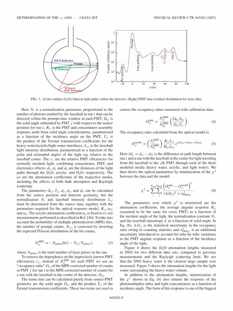
We measured the optical parameters using a pulsed nitrogenlaser source (the “laserball”) whose light was transmitted intothe detector through an optical fiber and diffused in a smallsphere containing 50-µm-diameter glass beads suspendedin a silicon gel. In addition to the primary wavelength of337.1 nm, a series of dyes provided additional wavelengths of365, 386, 420, 500, and 620 nm. These values were chosen toprovide good coverage over the range of detectable Cherenkovwavelengths. The left panel of Fig. 3 illustrates the variousoptical paths taken by the light for the source at the center of thedetector, and the right panel shows the measured distribution ofthe differences between PMT hit times and the laserball triggertime, corrected for photon time of flight (the “time-residualdistribution”). As the figure shows, the prompt window of thetime residuals is centered on the peak at t = 0, and severalother peaks including the reflections off the acrylic and thePMT array are indicated.
As with nearly all SNO calibration sources, the laserball canbe deployed almost anywhere in two orthogonal planes withinthe AV, as well as outside the vessel along a few vertical axes.For the data scans used to determine the optical parameters,we collected data 4 times with the laserball at the centerand 18 times off-center at radii between 100 and 500 cm.Each of the central-position data collections was done withfour different azimuthal orientations of the laserball to helpunderstand anisotropies in its light output. We kept the laserintensity relatively low (typically only about 5% of the PMTsregistered hits for each laser pulse) so that the corrections thatwe applied to account for multiple photons hitting a singletube were small.
The optical model used to predict the number of promptcounts, Nij , observed in PMT j in a given run i, within the±4 ns window, is parametrized as follows:
Nij = Ni�ijRijTijLij εj e−(ddαd+daαa+dhαh). (2)
045502-8
DETERMINATION OF THE νe AND . . . . I DATA SET PHYSICAL REVIEW C 75, 045502 (2007)
t (ns)−20 0 20 40 60 80 100
Cou
nts
(Arb
itra
ry u
nits
)
10−5
10−4
10−3
10−2
10−1
1
Pre
pul
sing
Pro
mpt
Lat
e pu
lsin
g
Lat
e pu
lsin
g
AV
PS
UP
35 D
egre
e
PromptPSUP Reflection
AV Reflection
35 DegreePMT Reflection
FIG. 3. (Color online) (Left) Optical light paths within the detector. (Right) PMT time residual distribution for laser data.
Here Ni is a normalization parameter, proportional to thenumber of photons emitted by the laserball in run i that can bedetected within the prompt-time window at each PMT; �ij isthe solid angle subtended by PMT j with respect to the sourceposition for run i; Rij is the PMT and concentrator assemblyresponse aside from solid angle considerations, parametrizedas a function of the incidence angle on the PMT; Tij isthe product of the Fresnel transmission coefficients for theheavy-water/acrylic/light-water interfaces; Lij is the laserballlight intensity distribution, parametrized as a function of thepolar and azimuthal angles of the light ray relative to thelaserball center. The εj are the relative PMT efficiencies fornormally incident light, combining concentrator, PMT, andelectronics effects; dd, da and dh are the distances of the lightpaths through the D2O, acrylic, and H2O, respectively. Theαs are the attenuation coefficients of the respective media,including the effects of both bulk absorption and Rayleighscattering.
The parameters �ij , Tij , da, dd , and dh can be calculatedfrom the source position and detector geometry, but thenormalization Ni and laserball intensity distribution Lij
must be determined from the source data, together with theparameters required for the optical response model, Rij , αd ,and αh. The acrylic attenuation coefficient αa is fixed to ex situmeasurements performed as described in Ref. [46]. To take intoaccount the probability of multiple photoelectron (MPE) hits,the number of prompt counts, Nij , is corrected by invertingthe expected Poisson distribution of the hit counts,
NMPEij = −Npulsesln(1 − Nij/Npulses), (3)
where Npulses is the total number of laser pulses in the run.To remove the dependence on the imprecisely known PMT
efficiencies εj , instead of NMPEij for each PMT we use an
“occupancy ratio” Oij of the MPE-corrected number of countsin PMT j for run i to the MPE-corrected number of counts fora run with the laserball in the center of the detector, O0j .
The terms that can be calculated purely from source-PMTgeometry are the solid angle �ij and the product Tij of theFresnel transmission coefficients. These two terms are used to
correct the occupancy ratios measured with calibration data:
Odataij = NMPE
ij
NMPE0j
(�0j T0j
�ijTij
). (4)
The occupancy ratio calculated from the optical model is
Omodelij =
(NMPE
i
NMPE0
)RijLij
R0jL0j
eδddαd+δdaαa+δdhαh . (5)
Here δdx = dij − di0 is the difference in path length betweenrun i and a run with the laserball in the center for light travelingfrom the laserball to the j th PMT through each of the threemodeled media (heavy water, acrylic, and light water). Wethen derive the optical parameters by minimization of the χ2
between the data and the model:
χ2 =Nruns∑
i
NPMT∑j
(Odata
ij − Omodelij
)2
(�Oij )2 + σ 2PMTij
. (6)
The parameters over which χ2 is minimized are theattenuation coefficients, the average angular response Rij
(assumed to be the same for every PMT) as a function ofthe incident angle of the light, the normalization constant Ni ,and the laserball anisotropy L as a function of solid angle. InEq. (6), �Oij is the statistical uncertainty in the occupancyratio owing to counting statistics and σ 2
PMTij is an additionaluncertainty introduced to account for tube-by-tube variationsin the PMT angular response as a function of the incidenceangle of the light.
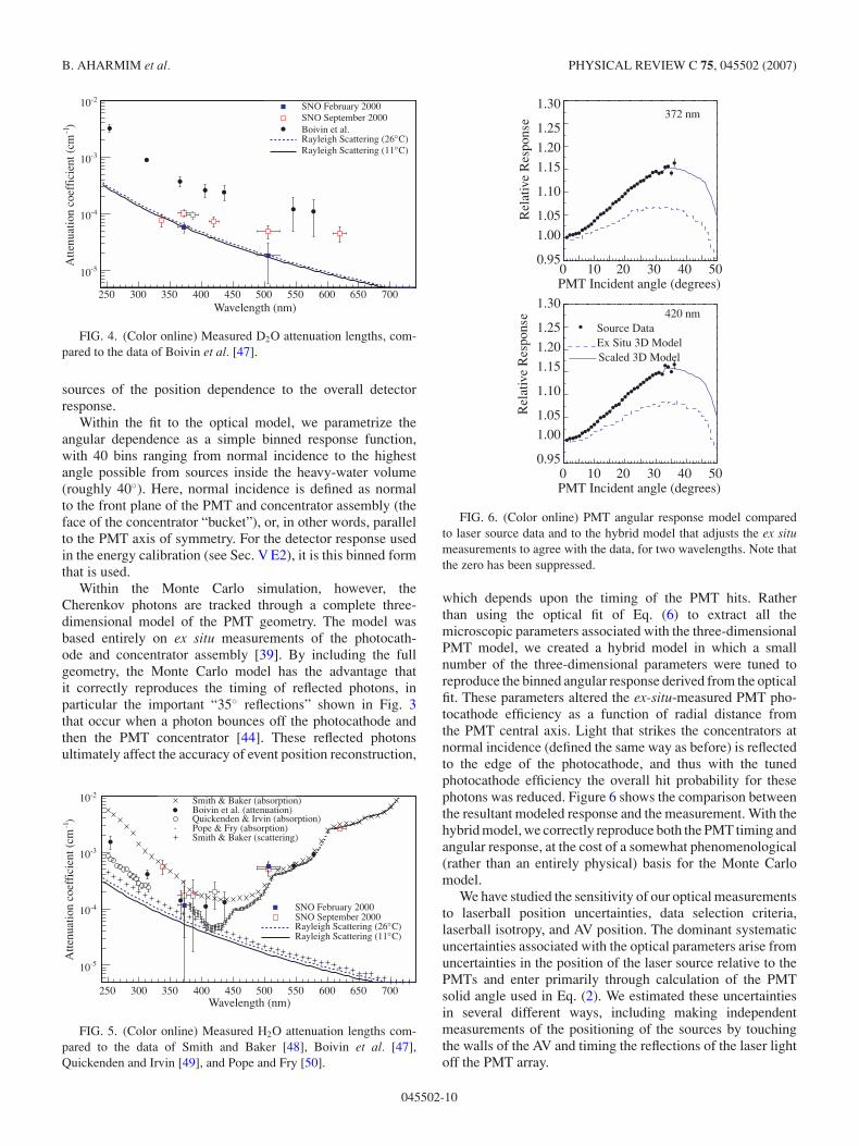
Figure 4 shows the D2O attenuation lengths measuredin SNO for two different data sets, compared to previousmeasurements and the Rayleigh scattering limit. We seethat the SNO heavy water is the clearest large sample evermeasured. Figure 5 shows the attenuation lengths for the lightwater surrounding the heavy-water volume.
In addition to the attenuation lengths, minimization ofthe χ2 shown in Eq. (6) also returns the response of thephotomultiplier tubes and light concentrators as a function ofincidence angle. The form of this response is one of the biggest
045502-9
B. AHARMIM et al. PHYSICAL REVIEW C 75, 045502 (2007)
Wavelength (nm)250 300 350 400 450 500 550 600 650 700
)-1
Atte
nuat
ion
coef
fici
ent (
cm
-510
-410
-310
-210 SNO February 2000SNO September 2000Boivin et al.
C)°Rayleigh Scattering (26 C)°Rayleigh Scattering (11
FIG. 4. (Color online) Measured D2O attenuation lengths, com-pared to the data of Boivin et al. [47].
sources of the position dependence to the overall detectorresponse.
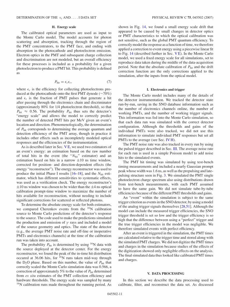
Within the fit to the optical model, we parametrize theangular dependence as a simple binned response function,with 40 bins ranging from normal incidence to the highestangle possible from sources inside the heavy-water volume(roughly 40◦). Here, normal incidence is defined as normalto the front plane of the PMT and concentrator assembly (theface of the concentrator “bucket”), or, in other words, parallelto the PMT axis of symmetry. For the detector response usedin the energy calibration (see Sec. V E2), it is this binned formthat is used.
Within the Monte Carlo simulation, however, theCherenkov photons are tracked through a complete three-dimensional model of the PMT geometry. The model wasbased entirely on ex situ measurements of the photocath-ode and concentrator assembly [39]. By including the fullgeometry, the Monte Carlo model has the advantage thatit correctly reproduces the timing of reflected photons, inparticular the important “35◦ reflections” shown in Fig. 3that occur when a photon bounces off the photocathode andthen the PMT concentrator [44]. These reflected photonsultimately affect the accuracy of event position reconstruction,
Wavelength (nm)250 300 350 400 450 500 550 600 650 700
)-1
Atte
nuat
ion
coef
fici
ent (
cm
-510
-410
-310
-210
SNO February 2000SNO September 2000
C)°Rayleigh Scattering (26 C)°Rayleigh Scattering (11
Smith & Baker (absorption)Boivin et al. (attenuation)Quickenden & Irvin (absorption)Pope & Fry (absorption)Smith & Baker (scattering)
FIG. 5. (Color online) Measured H2O attenuation lengths com-pared to the data of Smith and Baker [48], Boivin et al. [47],Quickenden and Irvin [49], and Pope and Fry [50].
Rel
ativ
e R
espo
nse
Rel
ativ
e R
espo
nse
0.95
0.95
1.00
1.00
1.05
1.05
1.10
1.10
1.15
1.15
1.20
1.20
1.25
1.25
1.30
1.30372 nm
PMT Incident angle (degrees)
PMT Incident angle (degrees)
0
0
10
10
20
20
30
30
40
40
50
50
420 nm
Scaled 3D ModelEx Situ 3D ModelSource Data
FIG. 6. (Color online) PMT angular response model comparedto laser source data and to the hybrid model that adjusts the ex situmeasurements to agree with the data, for two wavelengths. Note thatthe zero has been suppressed.
which depends upon the timing of the PMT hits. Ratherthan using the optical fit of Eq. (6) to extract all themicroscopic parameters associated with the three-dimensionalPMT model, we created a hybrid model in which a smallnumber of the three-dimensional parameters were tuned toreproduce the binned angular response derived from the opticalfit. These parameters altered the ex-situ-measured PMT pho-tocathode efficiency as a function of radial distance fromthe PMT central axis. Light that strikes the concentrators atnormal incidence (defined the same way as before) is reflectedto the edge of the photocathode, and thus with the tunedphotocathode efficiency the overall hit probability for thesephotons was reduced. Figure 6 shows the comparison betweenthe resultant modeled response and the measurement. With thehybrid model, we correctly reproduce both the PMT timing andangular response, at the cost of a somewhat phenomenological(rather than an entirely physical) basis for the Monte Carlomodel.
We have studied the sensitivity of our optical measurementsto laserball position uncertainties, data selection criteria,laserball isotropy, and AV position. The dominant systematicuncertainties associated with the optical parameters arise fromuncertainties in the position of the laser source relative to thePMTs and enter primarily through calculation of the PMTsolid angle used in Eq. (2). We estimated these uncertaintiesin several different ways, including making independentmeasurements of the positioning of the sources by touchingthe walls of the AV and timing the reflections of the laser lightoff the PMT array.
045502-10
DETERMINATION OF THE νe AND . . . . I DATA SET PHYSICAL REVIEW C 75, 045502 (2007)
H. Energy scale
The calibrated optical parameters are used as input tothe Monte Carlo model. The model accounts for photonscattering and absorption, tracking through the region ofthe PMT concentrators, to the PMT face, and ending withabsorption in the photocathode and photoelectron emission.Electron optics in the PMT and subsequent charge collectionand discrimination are not modeled, but an overall efficiencyfor these processes is included as a probability for a givenphotoelectron to produce a PMT hit. This probability is definedas
Phit = εcεt , (7)
where εc is the efficiency for collecting photoelectrons pro-duced at the photocathode onto the first PMT dynode (∼70%)and εt is the fraction of PMT pulses that generate a hitafter passing through the electronics chain and discriminator(approximately 80% for 1/4 photoelectron threshold), so thatPhit ≈ 0.56. The probability Phit thus sets the detector’s“energy scale” and allows the model to correctly predictthe number of detected PMT hits per MeV given an event’slocation and direction. Phenomenologically, the determinationof Phit corresponds to determining the average quantum anddetection efficiency of the PMT array, though in practice itincludes other effects such as incompletely modeled opticalresponses and the efficiencies of the instrumentation.
As is described later in Sec. V E, we used two estimators ofan event’s energy: an estimation based on the raw numberof total hits in the event (the “Nhit” estimator) and anestimation based on hits in a narrow ±10 ns time window,corrected for position- and direction-dependent effects (theenergy “reconstructor”). The energy reconstructor was used toproduce the initial Phase I results [16–18], and the Nhit esti-mator, which has different sensitivities to systematic effects,was used as a verification check. The energy reconstructor’s±10 ns window was chosen to be wider than the ±4 ns opticalcalibration prompt-time window to maximize the number ofhits available for reconstruction, without needing to includesignificant corrections for scattered or reflected photons.
To determine the absolute energy scale for both estimators,we compared Cherenkov events from the 16N calibrationsource to Monte Carlo predictions of the detector’s responseto the source. The code used to make the predictions simulatedthe production and emission of γ rays and included a modelof the source geometry and optics. The state of the detector(e.g., the average PMT noise rate and off-line or inoperativePMTs and electronics channels) at the time of the calibrationrun was taken into account.
The probability Phit is determined by using 16N data withthe source deployed at the detector center. For the energyreconstructor, we found the peak of the in-time hit distributionoccured at 36.06 hits, for 16N runs taken mid-way throughthe D2O phase. Based on this number, the value of Phit thatcorrectly scaled the Monte Carlo simulation data was 0.566, acorrection of approximately 5% to the value of Phit determinedfrom ex situ estimates of the PMT collection efficiency andhardware thresholds. The energy scale was sampled by many16N calibration runs made throughout the running period. As
shown in Fig. 14, we found a small energy scale drift thatappeared to be caused by small changes in detector opticsor PMT characteristics to which the optical calibration wasnot sensitive, such as the global PMT quantum efficiency. Tocorrectly model the response as a function of time, we thereforeapplied a correction to event energy using a piecewise linear fitto Fig. 14 (described further in Sec. V E). In the Monte Carlomodel, we used a fixed energy scale for all simulations, set toreproduce data taken during the middle of the data-acquisitionperiod. Note that the absolute calibration of Phit and the driftcorrection function are the only corrections applied to thesimulation, after the inputs from the optical model.
I. Electronics and trigger
The Monte Carlo model includes many of the details ofthe detector instrumentation. We tracked the detector staterun-by-run, saving in the SNO database information such asthe number of electronics channels online, the number ofworking PMTs, and the number of working trigger signals.This information was fed into the Monte Carlo simulation, sothat each data run was simulated with the correct detectorconfiguration. Although the thresholds and gains of theindividual PMTs were also tracked, we did not use thisinformation to simulate individual PMT responses but set allPMTs to the average (see Sec. IV H).
The PMT noise rate was also tracked in every run by usingthe pulsed trigger described in Sec. III. The average noise ratefor each run is used in a simple Poisson model to add noisehits to the simulated events.
The PMT hit timing was simulated by using test-benchtiming measurements and included a nearly Gaussian promptpeak whose width was 1.6 ns, as well as the prepulsing and late-pulsing structure seen in Fig. 3. We simulated the PMT singlephotoelectron charge spectrum also using distributions drawnfrom test-bench measurements, with each PMT assumedto have the same gain. We did not simulate tube-by-tubeefficiencies because of the different PMT thresholds and gains.
An “event” within the simulation is subject to the sametrigger criterion as events in the SNO detector, by using a modelof the analog trigger signals themselves [28,51]. Although themodel can include the measured trigger efficiencies, the SNOtrigger threshold is set so low and the trigger efficiency is sohigh that the difference between using a “perfect” trigger andthe true trigger efficiencies in the model was negligible. Wetherefore simulated events with perfect efficiency.
After an event is triggered in the simulation, the PMT timesare calculated relative to the trigger time and stored along withthe simulated PMT charges. We did not digitize the PMT timesand charges in the simulation because studies of the effects ofthe digitization showed only negligible effects on the analysis.The final simulated data thus looked like calibrated PMT timesand charges.
V. DATA PROCESSING
In this section we describe the data processing used tocalibrate, filter, and reconstruct the data set. As discussed
045502-11
B. AHARMIM et al. PHYSICAL REVIEW C 75, 045502 (2007)
in Sec. II and shown in Table XXVI, we created multipledistinct methods for all major analysis components. In thefollowing we discuss the multiple methods used for identifi-cation and removal of instrumental backgrounds, position anddirection reconstruction, and energy estimation. We leave theestimation of the numbers of residual background events toSec. VII.
A. Raw data
Each event recorded by the SNO detector contains severalitems of “header” information: the trigger ID number, a wordspecifying which trigger or triggers fired in the event, themaster clock time, and an absolute clock time synchronizedto the GPS system. The GPS system provides time with aresolution of 100 ns and an accuracy of ∼300 ns. For each hitchannel three digitized charges (a high-gain, short-integration-time charge; a high-gain, long-integration-time charge; anda low-gain, long-integration-time charge) and one time arerecorded. All hit times are relative to the time of arrival of theglobal trigger.
B. Charge and timing calibrations
To convert the digitized charges and times to values that canbe used in reconstruction and energy calibration, we subtractedpedestal values and converted the times from ADC countsto nanoseconds. The time conversion was done by linearlyinterpolating between 10 precisely measured pulser calibrationtimes. The digital resolution for the times was approximately0.1 ns, less than 1/10 that of the intrinsic PMT time reso-lution. The charges were not converted into picocoulombsor photoelectrons, but left as pedestal-subtracted ADC countvalues.
The pedestals and timing slopes were measured twiceweekly, and during data processing we applied the mostrecently measured set of calibrations. The pedestals were ex-tremely stable—the variations from calibration to calibrationwere typically as small as could be measured (below one ADCcount). The output of the pedestal and time calibration included
quality control flags that we used to reject channels that werenoticeably bad or came from boards that had been replacedbut not yet calibrated.
In addition to the pedestals and slopes applied to thedigitized times, we also measured and subtracted the globalchannel-to-channel timing offsets (caused by differencesin PMT transit times and small variations in signal pathlengths) using data from the laserball source described inSec. IV G. The laserball data also provided us with a charge-dependent correction to the measured PMT times, which wasnecessary to account for the variation in the rise time of thePMT pulses.
As was discussed in Sec. III, during the data-acquisitionperiod we discovered two problems with the charge and timingcalibrations. The first problem was the slow developmentof nonlinearities in the time- and charge-digitizing ADCs.Although we ultimately developed a hardware fix for theADCs, for data taken before the fix was implemented weapplied the quality control flags just discussed to reject affectedchannels.
The second problem was the small rate dependence of thetime and charge pedestal values—the pedestal calibrationswere typically taken at high rate while the actual neutrinodata were low rate, and therefore the “true” pedestal neededfor the neutrino data could be a few counts different from thecalibrated pedestal value. We developed a hardware solution tomitigate this problem, too, but also adjusted the time pedestalof each channel off-line based upon the time since it lastrecorded a hit. This adjustment removed most of the problem,but for nearly all important calibrations (such as energyscale or the reconstruction of event position) we used radioac-tive source data taken at both high and low rates to ensure therewere no residual effects. The rate dependence of the chargemeasurement was not corrected, but, as described later inSec. V E2, the overall analysis was designed to depend onlyweakly on the charge measurement.
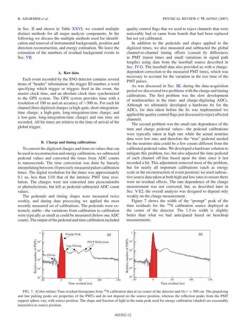
Figure 7 shows the width of the “prompt” peak of thetime residuals for the 16N calibration source deployed atthe center of the detector. The 1.5-ns width is slightlybetter than what we had anticipated based on benchtopmeasurements.
Time residual [ns]-50 0 50 100 150
Rel
ativ
e nu
mbe
r of
PM
Ts
10-5
10-4
10-3
10-2
10-1
1 (b)
Time residual [ns]-50 0 50 100 150
Rel
ativ
e nu
mbe
r of
PM
Ts
10-5
10-4
10-3
10-2
10-1
1 (a)
Pre-Pulsing
Late Pulsing
Prompt Peak
PSUP Reflections
FIG. 7. (Color online) Time residual histograms from 16N calibration data at (a) center of the detector and (b) r = 500 cm. The prepulsingand late pulsing peaks are properties of the PMTs and do not depend on the source position, whereas the reflection peaks from the PMTsupport sphere vary with source position. The shape and fraction of light in the main peak used for energy calibration (shaded) are reasonablyinsensitive to source position.
045502-12
DETERMINATION OF THE νe AND . . . . I DATA SET PHYSICAL REVIEW C 75, 045502 (2007)
C. Instrumental background cuts
In addition to neutrino interactions, cosmic rays, andradioactive decays, the SNO detector also collects and recordsmany background events produced by the detector instrumen-tation itself. They have several sources and span the energyrange of interest for solar neutrino analysis. Although theseevents are relatively easy to distinguish from neutrino events,because of their much higher frequency a high rejectionfraction is needed to ensure they do not contaminate thefinal data sample. More information on the instrumentalbackgrounds and the cuts used to remove them can be foundin Appendix B and Refs. [52,53].
There are four distinct classes of instrumental backgroundsources:
(i) Photomultiplier tubes: Small discharges within a PMTcan produce detectable light. Although for a singlePMT this occurs rarely (roughly once each week),integrated over the entire array we see roughly one such“flasher” event each minute. Further, seismic activitywithin the mine—either natural or mining related—cancause thousands of PMTs to flash within several tens ofmilliseconds.
The PMTs can also produce light from high-voltagebreakdown in their connectors or bases. Such events lightup nearly the entire PMT array and are accompanied byelectronic pickup in neighboring electronic channels andcrates.
(ii) External light: Light outside the PMT array can generatedetectable hits by entering through the neck region of theAV or through the backs of the PMTs. For example, staticdischarges in the neck of the AV, and at the boundaryof the acrylic, nitrogen cover gas, and the water surface,can produce hits at the bottom of the PMT array.
(iii) Electronic pickup: Activity near the electronics rackscausing electronic noise can produce radiative pickupin many channels at once. Readout of a crate canoccasionally produce hits confined to a single card inan electronics crate.
(iv) Acrylic backgrounds: The acrylic vessel itself sometimesemits isotropically distributed light at several locations;this light does not appear to be associated with anyradioactivity.
To remove the vast majority of these events efficiently,we developed a suite of “low-level” cuts that are applied to thedata set before reconstruction (see Appendix B). The cuts arebased on information such as the distribution of PMT chargemeasurements, the total integrated charge, the time distributionof PMT hits, the interevent timing, the spatial distributionof PMT hits, and the firing of veto PMTs installed in theneck region and outside the PMT support sphere. “Flasher”events, for example, are characterized by a high charge in theoffending PMT; electronic pickup events have many channelswhose integrated charge is near the pedestal level. The cutswere designed individually as coarse filters to remove themost obvious background events, but the combination ofthe cuts removed nearly all the instrumental backgrounds (seeSec. VII A) before the more sophisticated stages of the
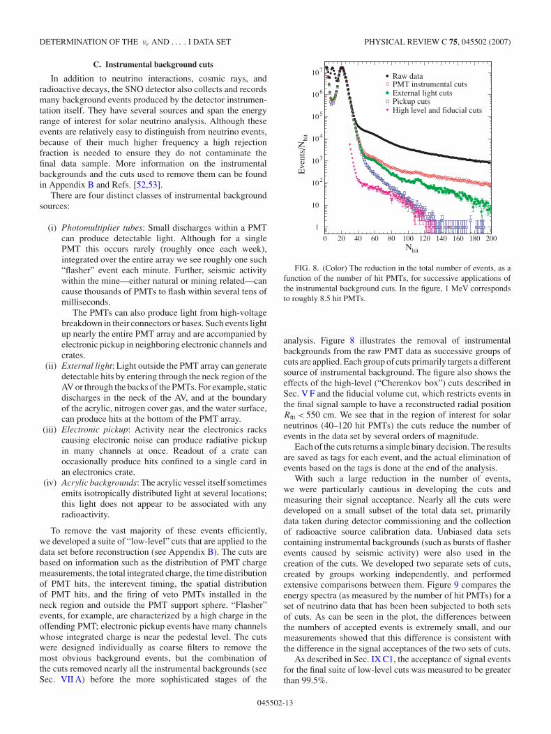
Raw dataPMT instrumental cutsExternal light cutsPickup cutsHigh level and fiducial cuts
Nhit
Eve
nts/
Nhi
t
1
10
102
103
104
105
106
107
0 20 40 60 80 100 120 140 160 180 200
FIG. 8. (Color) The reduction in the total number of events, as afunction of the number of hit PMTs, for successive applications ofthe instrumental background cuts. In the figure, 1 MeV correspondsto roughly 8.5 hit PMTs.
analysis. Figure 8 illustrates the removal of instrumentalbackgrounds from the raw PMT data as successive groups ofcuts are applied. Each group of cuts primarily targets a differentsource of instrumental background. The figure also shows theeffects of the high-level (“Cherenkov box”) cuts described inSec. V F and the fiducial volume cut, which restricts events inthe final signal sample to have a reconstructed radial positionRfit < 550 cm. We see that in the region of interest for solarneutrinos (40–120 hit PMTs) the cuts reduce the number ofevents in the data set by several orders of magnitude.
Each of the cuts returns a simple binary decision. The resultsare saved as tags for each event, and the actual elimination ofevents based on the tags is done at the end of the analysis.
With such a large reduction in the number of events,we were particularly cautious in developing the cuts andmeasuring their signal acceptance. Nearly all the cuts weredeveloped on a small subset of the total data set, primarilydata taken during detector commissioning and the collectionof radioactive source calibration data. Unbiased data setscontaining instrumental backgrounds (such as bursts of flasherevents caused by seismic activity) were also used in thecreation of the cuts. We developed two separate sets of cuts,created by groups working independently, and performedextensive comparisons between them. Figure 9 compares theenergy spectra (as measured by the number of hit PMTs) for aset of neutrino data that has been been subjected to both setsof cuts. As can be seen in the plot, the differences betweenthe numbers of accepted events is extremely small, and ourmeasurements showed that this difference is consistent withthe difference in the signal acceptances of the two sets of cuts.
As described in Sec. IX C1, the acceptance of signal eventsfor the final suite of low-level cuts was measured to be greaterthan 99.5%.
045502-13
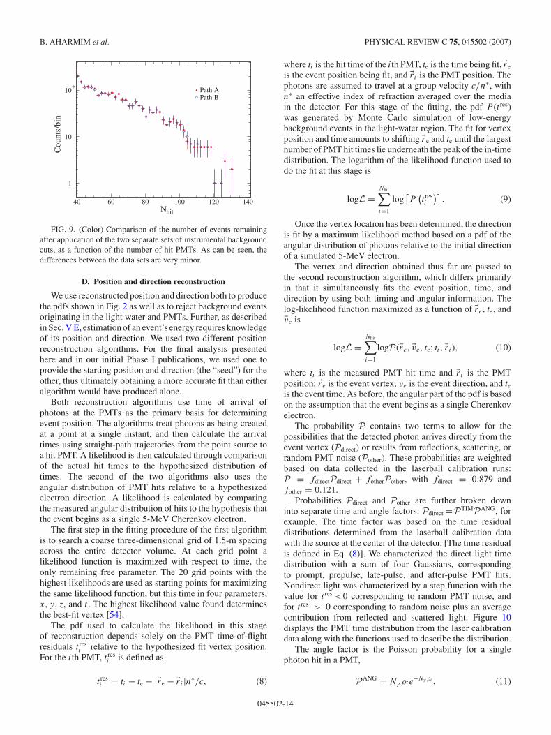
B. AHARMIM et al. PHYSICAL REVIEW C 75, 045502 (2007)
Path APath B
Nhit
Cou
nts/
bin
1
10
102
40 60 80 100 120 140
FIG. 9. (Color) Comparison of the number of events remainingafter application of the two separate sets of instrumental backgroundcuts, as a function of the number of hit PMTs. As can be seen, thedifferences between the data sets are very minor.
D. Position and direction reconstruction
We use reconstructed position and direction both to producethe pdfs shown in Fig. 2 as well as to reject background eventsoriginating in the light water and PMTs. Further, as describedin Sec. V E, estimation of an event’s energy requires knowledgeof its position and direction. We used two different positionreconstruction algorithms. For the final analysis presentedhere and in our initial Phase I publications, we used one toprovide the starting position and direction (the “seed”) for theother, thus ultimately obtaining a more accurate fit than eitheralgorithm would have produced alone.
Both reconstruction algorithms use time of arrival ofphotons at the PMTs as the primary basis for determiningevent position. The algorithms treat photons as being createdat a point at a single instant, and then calculate the arrivaltimes using straight-path trajectories from the point source toa hit PMT. A likelihood is then calculated through comparisonof the actual hit times to the hypothesized distribution oftimes. The second of the two algorithms also uses theangular distribution of PMT hits relative to a hypothesizedelectron direction. A likelihood is calculated by comparingthe measured angular distribution of hits to the hypothesis thatthe event begins as a single 5-MeV Cherenkov electron.
The first step in the fitting procedure of the first algorithmis to search a coarse three-dimensional grid of 1.5-m spacingacross the entire detector volume. At each grid point alikelihood function is maximized with respect to time, theonly remaining free parameter. The 20 grid points with thehighest likelihoods are used as starting points for maximizingthe same likelihood function, but this time in four parameters,x, y, z, and t . The highest likelihood value found determinesthe best-fit vertex [54].
The pdf used to calculate the likelihood in this stageof reconstruction depends solely on the PMT time-of-flightresiduals t res
i relative to the hypothesized fit vertex position.For the ith PMT, t res
i is defined as
t resi = ti − te − |re − ri |n∗/c, (8)
where ti is the hit time of the ith PMT, te is the time being fit, re
is the event position being fit, and ri is the PMT position. Thephotons are assumed to travel at a group velocity c/n∗, withn∗ an effective index of refraction averaged over the mediain the detector. For this stage of the fitting, the pdf P (t res)was generated by Monte Carlo simulation of low-energybackground events in the light-water region. The fit for vertexposition and time amounts to shifting re and te until the largestnumber of PMT hit times lie underneath the peak of the in-timedistribution. The logarithm of the likelihood function used todo the fit at this stage is
logL =Nhit∑i=1
log[P
(t resi
)]. (9)
Once the vertex location has been determined, the directionis fit by a maximum likelihood method based on a pdf of theangular distribution of photons relative to the initial directionof a simulated 5-MeV electron.
The vertex and direction obtained thus far are passed tothe second reconstruction algorithm, which differs primarilyin that it simultaneously fits the event position, time, anddirection by using both timing and angular information. Thelog-likelihood function maximized as a function of re, te, andve is
logL =Nhit∑i=1
logP(re, ve, te; ti , ri), (10)
where ti is the measured PMT hit time and ri is the PMTposition; re is the event vertex, ve is the event direction, and teis the event time. As before, the angular part of the pdf is basedon the assumption that the event begins as a single Cherenkovelectron.
The probability P contains two terms to allow for thepossibilities that the detected photon arrives directly from theevent vertex (Pdirect) or results from reflections, scattering, orrandom PMT noise (Pother). These probabilities are weightedbased on data collected in the laserball calibration runs:P = fdirectPdirect + fotherPother, with fdirect = 0.879 andfother = 0.121.
Probabilities Pdirect and Pother are further broken downinto separate time and angle factors: Pdirect =PTIMPANG, forexample. The time factor was based on the time residualdistributions determined from the laserball calibration datawith the source at the center of the detector. [The time residualis defined in Eq. (8)]. We characterized the direct light timedistribution with a sum of four Gaussians, correspondingto prompt, prepulse, late-pulse, and after-pulse PMT hits.Nondirect light was characterized by a step function with thevalue for t res < 0 corresponding to random PMT noise, andfor t res > 0 corresponding to random noise plus an averagecontribution from reflected and scattered light. Figure 10displays the PMT time distribution from the laser calibrationdata along with the functions used to describe the distribution.
The angle factor is the Poisson probability for a singlephoton hit in a PMT,
PANG = Nγ ρie−Nγ ρi , (11)
045502-14
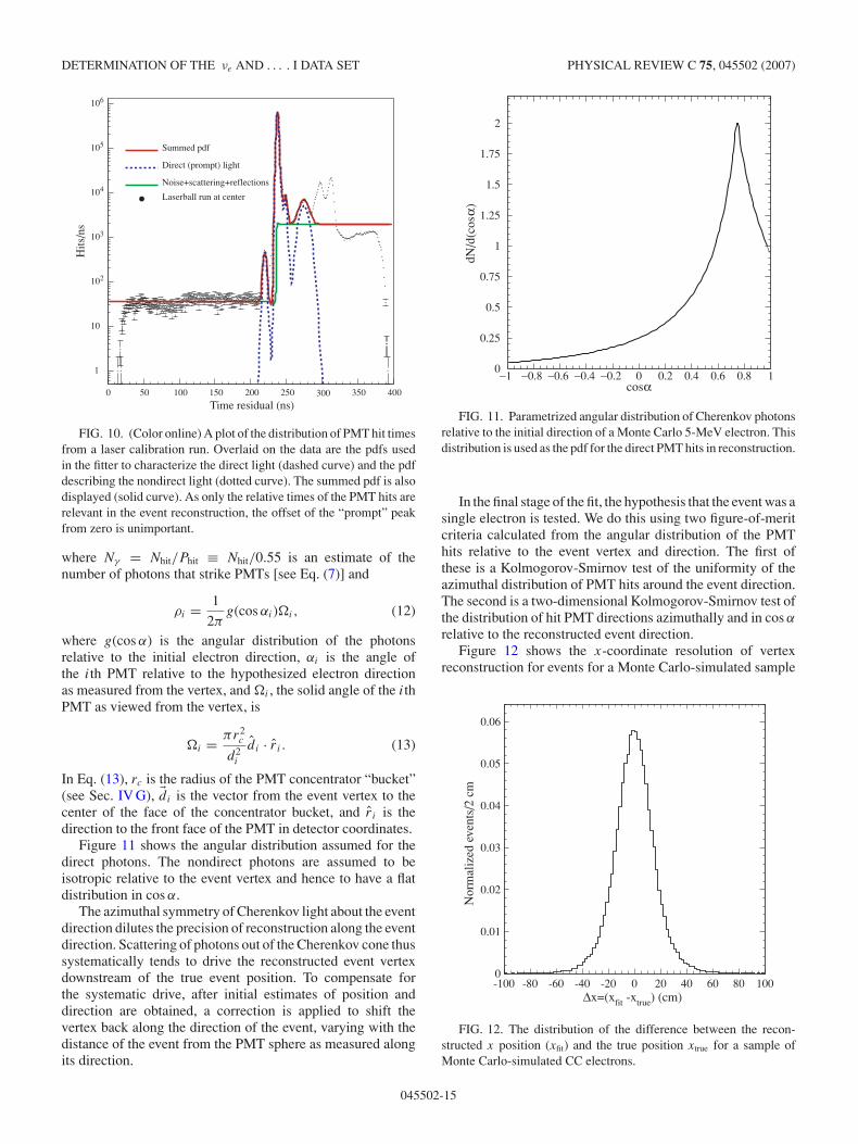
DETERMINATION OF THE νe AND . . . . I DATA SET PHYSICAL REVIEW C 75, 045502 (2007)
Noise+scattering+reflections
Laserball run at center
Direct (prompt) light
Summed pdf
Hits
/ns
Time residual (ns)
1
10
102
103
104
105
106
0 50 100 150 200 250 350300 400
FIG. 10. (Color online) A plot of the distribution of PMT hit timesfrom a laser calibration run. Overlaid on the data are the pdfs usedin the fitter to characterize the direct light (dashed curve) and the pdfdescribing the nondirect light (dotted curve). The summed pdf is alsodisplayed (solid curve). As only the relative times of the PMT hits arerelevant in the event reconstruction, the offset of the “prompt” peakfrom zero is unimportant.
where Nγ = Nhit/Phit ≡ Nhit/0.55 is an estimate of thenumber of photons that strike PMTs [see Eq. (7)] and
ρi = 1
2πg(cos αi)�i, (12)
where g(cos α) is the angular distribution of the photonsrelative to the initial electron direction, αi is the angle ofthe ith PMT relative to the hypothesized electron directionas measured from the vertex, and �i , the solid angle of the ithPMT as viewed from the vertex, is
�i = πr2c
d2i
d i · r i . (13)
In Eq. (13), rc is the radius of the PMT concentrator “bucket”(see Sec. IV G), di is the vector from the event vertex to thecenter of the face of the concentrator bucket, and r i is thedirection to the front face of the PMT in detector coordinates.
Figure 11 shows the angular distribution assumed for thedirect photons. The nondirect photons are assumed to beisotropic relative to the event vertex and hence to have a flatdistribution in cos α.
The azimuthal symmetry of Cherenkov light about the eventdirection dilutes the precision of reconstruction along the eventdirection. Scattering of photons out of the Cherenkov cone thussystematically tends to drive the reconstructed event vertexdownstream of the true event position. To compensate forthe systematic drive, after initial estimates of position anddirection are obtained, a correction is applied to shift thevertex back along the direction of the event, varying with thedistance of the event from the PMT sphere as measured alongits direction.
cosα
dN/d
(cos
α)
0
0.25
0.5
0.75
1
1.25
1.5
1.75
2
−1 −0.8 −0.6 −0.4 −0.2 0 0.2 0.4 0.6 0.8 1
FIG. 11. Parametrized angular distribution of Cherenkov photonsrelative to the initial direction of a Monte Carlo 5-MeV electron. Thisdistribution is used as the pdf for the direct PMT hits in reconstruction.
In the final stage of the fit, the hypothesis that the event was asingle electron is tested. We do this using two figure-of-meritcriteria calculated from the angular distribution of the PMThits relative to the event vertex and direction. The first ofthese is a Kolmogorov-Smirnov test of the uniformity of theazimuthal distribution of PMT hits around the event direction.The second is a two-dimensional Kolmogorov-Smirnov test ofthe distribution of hit PMT directions azimuthally and in cos α
relative to the reconstructed event direction.Figure 12 shows the x-coordinate resolution of vertex
reconstruction for events for a Monte Carlo-simulated sample
∆x=(xfit -xtrue) (cm)
Nor
mal
ized
eve
nts/
2 cm
0
0.01
0.02
0.03
0.04
0.05
0.06
-100 -80 -60 -40 -20 0 20 40 60 80 100
FIG. 12. The distribution of the difference between the recon-structed x position (xfit) and the true position xtrue for a sample ofMonte Carlo-simulated CC electrons.
045502-15
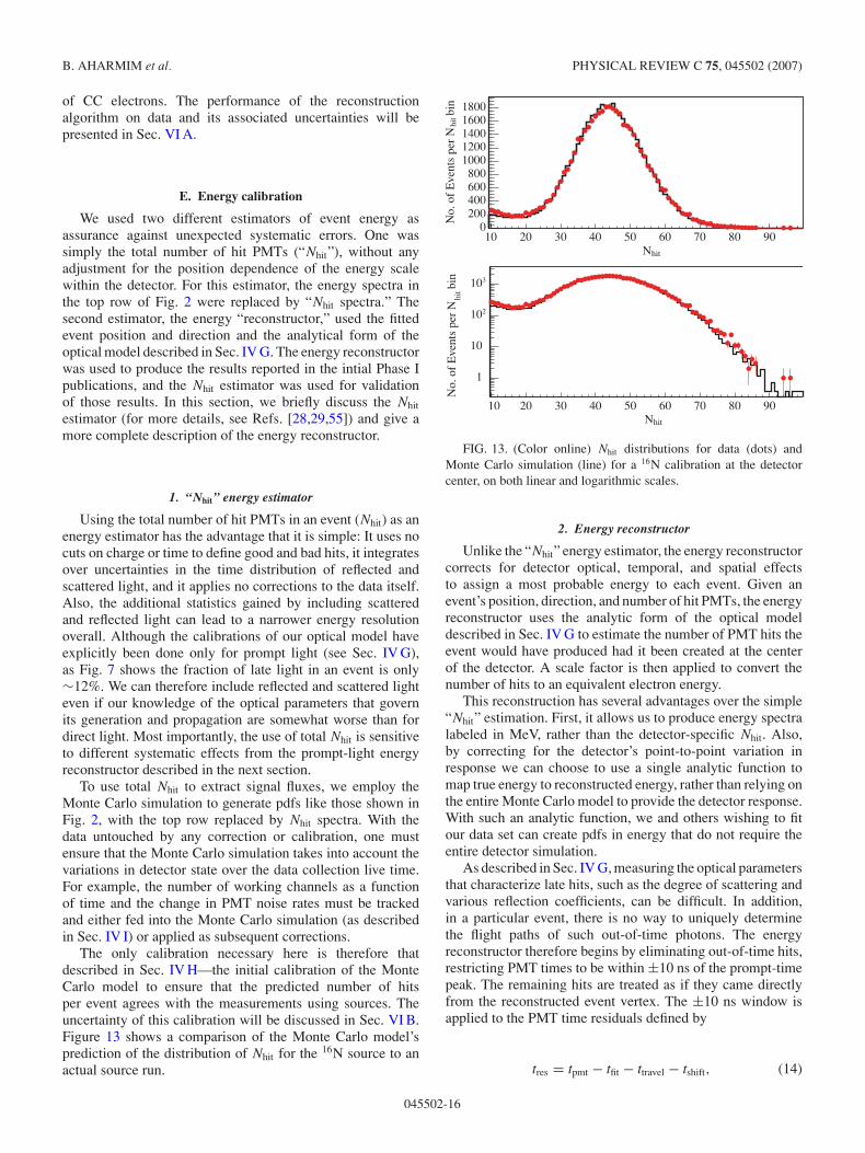
B. AHARMIM et al. PHYSICAL REVIEW C 75, 045502 (2007)
of CC electrons. The performance of the reconstructionalgorithm on data and its associated uncertainties will bepresented in Sec. VI A.
E. Energy calibration
We used two different estimators of event energy asassurance against unexpected systematic errors. One wassimply the total number of hit PMTs (“Nhit”), without anyadjustment for the position dependence of the energy scalewithin the detector. For this estimator, the energy spectra inthe top row of Fig. 2 were replaced by “Nhit spectra.” Thesecond estimator, the energy “reconstructor,” used the fittedevent position and direction and the analytical form of theoptical model described in Sec. IV G. The energy reconstructorwas used to produce the results reported in the intial Phase Ipublications, and the Nhit estimator was used for validationof those results. In this section, we briefly discuss the Nhit
estimator (for more details, see Refs. [28,29,55]) and give amore complete description of the energy reconstructor.
1. “Nhit” energy estimator
Using the total number of hit PMTs in an event (Nhit) as anenergy estimator has the advantage that it is simple: It uses nocuts on charge or time to define good and bad hits, it integratesover uncertainties in the time distribution of reflected andscattered light, and it applies no corrections to the data itself.Also, the additional statistics gained by including scatteredand reflected light can lead to a narrower energy resolutionoverall. Although the calibrations of our optical model haveexplicitly been done only for prompt light (see Sec. IV G),as Fig. 7 shows the fraction of late light in an event is only∼12%. We can therefore include reflected and scattered lighteven if our knowledge of the optical parameters that governits generation and propagation are somewhat worse than fordirect light. Most importantly, the use of total Nhit is sensitiveto different systematic effects from the prompt-light energyreconstructor described in the next section.
To use total Nhit to extract signal fluxes, we employ theMonte Carlo simulation to generate pdfs like those shown inFig. 2, with the top row replaced by Nhit spectra. With thedata untouched by any correction or calibration, one mustensure that the Monte Carlo simulation takes into account thevariations in detector state over the data collection live time.For example, the number of working channels as a functionof time and the change in PMT noise rates must be trackedand either fed into the Monte Carlo simulation (as describedin Sec. IV I) or applied as subsequent corrections.
The only calibration necessary here is therefore thatdescribed in Sec. IV H—the initial calibration of the MonteCarlo model to ensure that the predicted number of hitsper event agrees with the measurements using sources. Theuncertainty of this calibration will be discussed in Sec. VI B.Figure 13 shows a comparison of the Monte Carlo model’sprediction of the distribution of Nhit for the 16N source to anactual source run.
Nhit
10 20 30 40 50 60 70 80 90
No.
of
Eve
nts
per
N
bin
hit
0200400600800
10001200140016001800
Nhit
10 20 30 40 50 60 70 80 90
No.
of
Eve
nts
per
N
bin
hit
1
10
102
103
FIG. 13. (Color online) Nhit distributions for data (dots) andMonte Carlo simulation (line) for a 16N calibration at the detectorcenter, on both linear and logarithmic scales.
2. Energy reconstructor
Unlike the “Nhit” energy estimator, the energy reconstructorcorrects for detector optical, temporal, and spatial effectsto assign a most probable energy to each event. Given anevent’s position, direction, and number of hit PMTs, the energyreconstructor uses the analytic form of the optical modeldescribed in Sec. IV G to estimate the number of PMT hits theevent would have produced had it been created at the centerof the detector. A scale factor is then applied to convert thenumber of hits to an equivalent electron energy.
This reconstruction has several advantages over the simple“Nhit” estimation. First, it allows us to produce energy spectralabeled in MeV, rather than the detector-specific Nhit. Also,by correcting for the detector’s point-to-point variation inresponse we can choose to use a single analytic function tomap true energy to reconstructed energy, rather than relying onthe entire Monte Carlo model to provide the detector response.With such an analytic function, we and others wishing to fitour data set can create pdfs in energy that do not require theentire detector simulation.
As described in Sec. IV G, measuring the optical parametersthat characterize late hits, such as the degree of scattering andvarious reflection coefficients, can be difficult. In addition,in a particular event, there is no way to uniquely determinethe flight paths of such out-of-time photons. The energyreconstructor therefore begins by eliminating out-of-time hits,restricting PMT times to be within ±10 ns of the prompt-timepeak. The remaining hits are treated as if they came directlyfrom the reconstructed event vertex. The ±10 ns window isapplied to the PMT time residuals defined by
tres = tpmt − tfit − ttravel − tshift, (14)
045502-16
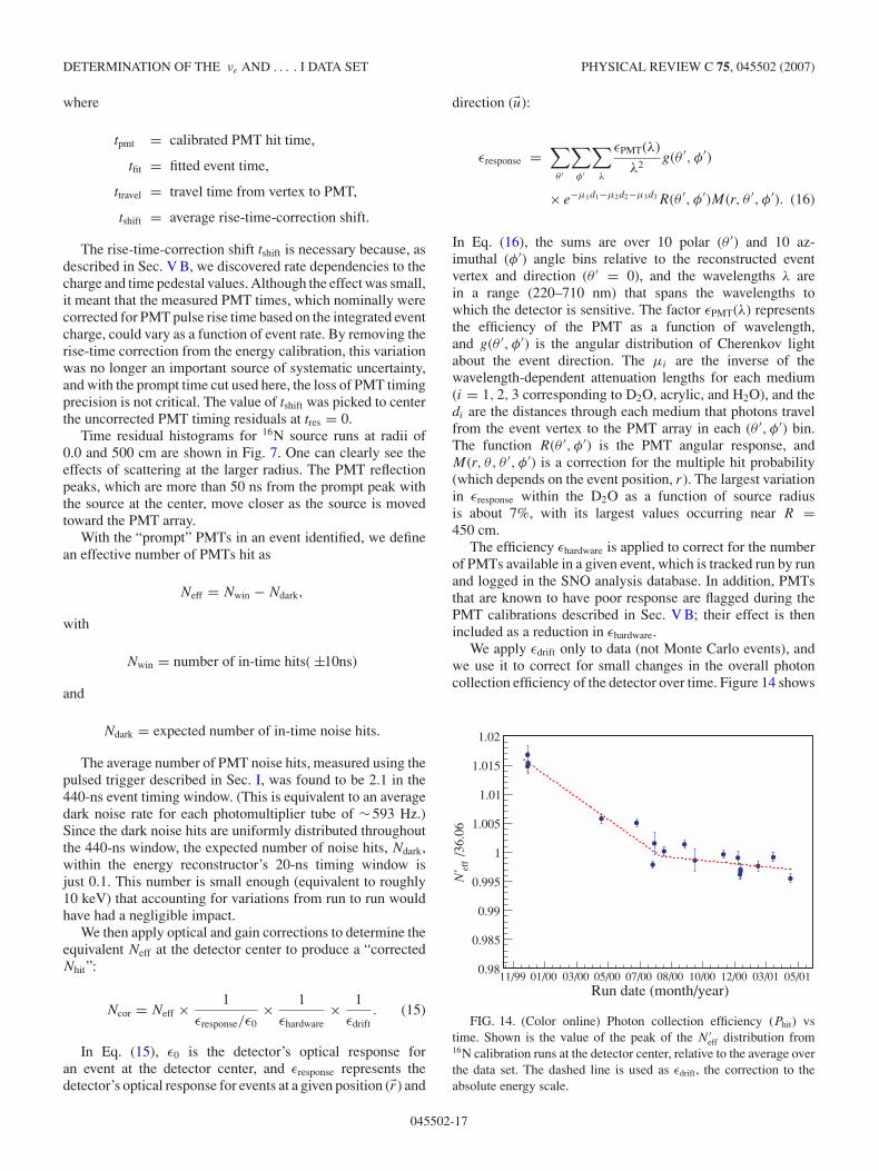
DETERMINATION OF THE νe AND . . . . I DATA SET PHYSICAL REVIEW C 75, 045502 (2007)
where
tpmt = calibrated PMT hit time,
tfit = fitted event time,
ttravel = travel time from vertex to PMT,
tshift = average rise-time-correction shift.
The rise-time-correction shift tshift is necessary because, asdescribed in Sec. V B, we discovered rate dependencies to thecharge and time pedestal values. Although the effect was small,it meant that the measured PMT times, which nominally werecorrected for PMT pulse rise time based on the integrated eventcharge, could vary as a function of event rate. By removing therise-time correction from the energy calibration, this variationwas no longer an important source of systematic uncertainty,and with the prompt time cut used here, the loss of PMT timingprecision is not critical. The value of tshift was picked to centerthe uncorrected PMT timing residuals at tres = 0.
Time residual histograms for 16N source runs at radii of0.0 and 500 cm are shown in Fig. 7. One can clearly see theeffects of scattering at the larger radius. The PMT reflectionpeaks, which are more than 50 ns from the prompt peak withthe source at the center, move closer as the source is movedtoward the PMT array.
With the “prompt” PMTs in an event identified, we definean effective number of PMTs hit as
Neff = Nwin − Ndark,
with
Nwin = number of in-time hits( ±10ns)
and
Ndark = expected number of in-time noise hits.
The average number of PMT noise hits, measured using thepulsed trigger described in Sec. I, was found to be 2.1 in the440-ns event timing window. (This is equivalent to an averagedark noise rate for each photomultiplier tube of ∼593 Hz.)Since the dark noise hits are uniformly distributed throughoutthe 440-ns window, the expected number of noise hits, Ndark,within the energy reconstructor’s 20-ns timing window isjust 0.1. This number is small enough (equivalent to roughly10 keV) that accounting for variations from run to run wouldhave had a negligible impact.
We then apply optical and gain corrections to determine theequivalent Neff at the detector center to produce a “correctedNhit”:
Ncor = Neff × 1
εresponse/ε0× 1
εhardware× 1
εdrift. (15)
In Eq. (15), ε0 is the detector’s optical response foran event at the detector center, and εresponse represents thedetector’s optical response for events at a given position (r) and
direction (u):
εresponse =∑θ ′
∑φ′
∑λ
εPMT(λ)
λ2g(θ ′, φ′)
× e−µ1d1−µ2d2−µ3d3R(θ ′, φ′)M(r, θ ′, φ′). (16)
In Eq. (16), the sums are over 10 polar (θ ′) and 10 az-imuthal (φ′) angle bins relative to the reconstructed eventvertex and direction (θ ′ = 0), and the wavelengths λ arein a range (220–710 nm) that spans the wavelengths towhich the detector is sensitive. The factor εPMT(λ) representsthe efficiency of the PMT as a function of wavelength,and g(θ ′, φ′) is the angular distribution of Cherenkov lightabout the event direction. The µi are the inverse of thewavelength-dependent attenuation lengths for each medium(i = 1, 2, 3 corresponding to D2O, acrylic, and H2O), and thedi are the distances through each medium that photons travelfrom the event vertex to the PMT array in each (θ ′, φ′) bin.The function R(θ ′, φ′) is the PMT angular response, andM(r, θ, θ ′, φ′) is a correction for the multiple hit probability(which depends on the event position, r). The largest variationin εresponse within the D2O as a function of source radiusis about 7%, with its largest values occurring near R =450 cm.
The efficiency εhardware is applied to correct for the numberof PMTs available in a given event, which is tracked run by runand logged in the SNO analysis database. In addition, PMTsthat are known to have poor response are flagged during thePMT calibrations described in Sec. V B; their effect is thenincluded as a reduction in εhardware.
We apply εdrift only to data (not Monte Carlo events), andwe use it to correct for small changes in the overall photoncollection efficiency of the detector over time. Figure 14 shows
Run date (month/year)11/99 01/00 03/00 05/00 07/00 08/00 10/00 12/00 03/01 05/01
/36.
06ef
fN
’
0.98
0.985
0.99
0.995
1
1.005
1.01
1.015
1.02
FIG. 14. (Color online) Photon collection efficiency (Phit) vstime. Shown is the value of the peak of the N ′
eff distribution from16N calibration runs at the detector center, relative to the average overthe data set. The dashed line is used as εdrift, the correction to theabsolute energy scale.
045502-17
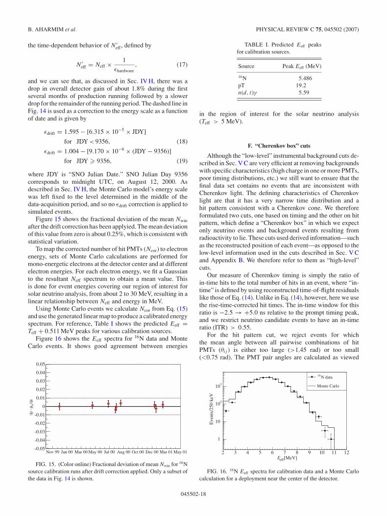
B. AHARMIM et al. PHYSICAL REVIEW C 75, 045502 (2007)
the time-dependent behavior of N ′eff , defined by
N ′eff = Neff × 1
εhardware, (17)
and we can see that, as discussed in Sec. IV H, there was adrop in overall detector gain of about 1.8% during the firstseveral months of production running followed by a slowerdrop for the remainder of the running period. The dashed line inFig. 14 is used as a correction to the energy scale as a functionof date and is given by
εdrift = 1.595 − [6.315 × 10⁻⁵ × JDY]
for JDY < 9356, (18)
εdrift = 1.004 − [9.170 × 10⁻⁶ × (JDY − 9356)]
for JDY � 9356, (19)
where JDY is “SNO Julian Date.” SNO Julian Day 9356corresponds to midnight UTC, on August 12, 2000. Asdescribed in Sec. IV H, the Monte Carlo model’s energy scalewas left fixed to the level determined in the middle of thedata-acquisition period, and so no εdrift correction is applied tosimulated events.
Figure 15 shows the fractional deviation of the mean Nwin
after the drift correction has been applyied. The mean deviationof this value from zero is about 0.25%, which is consistent withstatistical variation.
To map the corrected number of hit PMTs (Ncor) to electronenergy, sets of Monte Carlo calculations are performed formono-energetic electrons at the detector center and at differentelectron energies. For each electron energy, we fit a Gaussianto the resultant Neff spectrum to obtain a mean value. Thisis done for event energies covering our region of interest forsolar neutrino analysis, from about 2 to 30 MeV, resulting in alinear relationship between Neff and energy in MeV.
Using Monte Carlo events we calculate Ncor from Eq. (15)and use the generated linear map to produce a calibrated energyspectrum. For reference, Table I shows the predicted Eeff =Teff + 0.511 MeV peaks for various calibration sources.
Figure 16 shows the Eeff spectra for 16N data and MonteCarlo events. It shows good agreement between energies
Nov 99 Jan 00 Mar 00 May 00 Jul 00 Aug 00 Oct 00 Dec 00 Mar 01 May 01
µ)/ 0µ
-
µ(
-0.05
-0.04
-0.03
-0.02
-0.01
0
0.01
0.02
0.03
0.04
0.05
FIG. 15. (Color online) Fractional deviation of mean Nwin for 16Nsource calibration runs after drift correction applied. Only a subset ofthe data in Fig. 14 is shown.
TABLE I. Predicted Eeff peaksfor calibration sources.
Source Peak Eeff (MeV)
16N 5.486pT 19.2n(d, t)γ 5.59
in the region of interest for the solar neutrino analysis(Teff > 5 MeV).
F. “Cherenkov box” cuts
Although the “low-level” instrumental background cuts de-scribed in Sec. V C are very efficient at removing backgroundswith specific characteristics (high charge in one or more PMTs,poor timing distributions, etc.) we still want to ensure that thefinal data set contains no events that are inconsistent withCherenkov light. The defining characteristics of Cherenkovlight are that it has a very narrow time distribution and ahit pattern consistent with a Cherenkov cone. We thereforeformulated two cuts, one based on timing and the other on hitpattern, which define a “Cherenkov box” in which we expectonly neutrino events and background events resulting fromradioactivity to lie. These cuts used derived information—suchas the reconstructed position of each event—as opposed to thelow-level information used in the cuts described in Sec. V Cand Appendix B. We therefore refer to them as “high-level”cuts.
Our measure of Cherenkov timing is simply the ratio ofin-time hits to the total number of hits in an event, where “in-time” is defined by using reconstructed time-of-flight residualslike those of Eq. (14). Unlike in Eq. (14), however, here we usethe rise-time-corrected hit times. The in-time window for thisratio is −2.5 → +5.0 ns relative to the prompt timing peak,and we restrict neutrino candidate events to have an in-timeratio (ITR) > 0.55.
For the hit pattern cut, we reject events for whichthe mean angle between all pairwise combinations of hitPMTs (θij ) is either too large (>1.45 rad) or too small(<0.75 rad). The PMT pair angles are calculated as viewed
[MeV]effE2 3 4 5 6 7 8 9 10 11 12
Eve
nts/
250
keV
1
10
102
103
N data16
Monte Carlo
FIG. 16. 16N Eeff spectra for calibration data and a Monte Carlocalculation for a deployment near the center of the detector.
045502-18
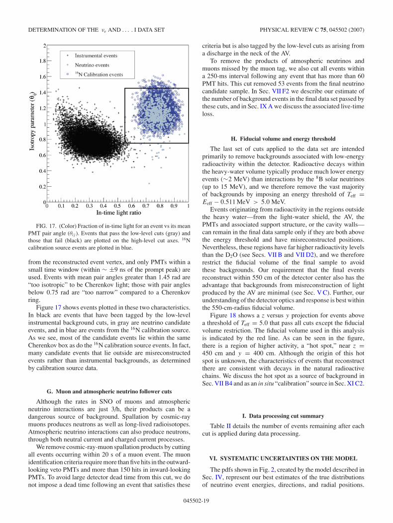
DETERMINATION OF THE νe AND . . . . I DATA SET PHYSICAL REVIEW C 75, 045502 (2007)
FIG. 17. (Color) Fraction of in-time light for an event vs its meanPMT pair angle (θij ). Events that pass the low-level cuts (gray) andthose that fail (black) are plotted on the high-level cut axes. 16Ncalibration source events are plotted in blue.
from the reconstructed event vertex, and only PMTs within asmall time window (within ∼ ±9 ns of the prompt peak) areused. Events with mean pair angles greater than 1.45 rad are“too isotropic” to be Cherenkov light; those with pair anglesbelow 0.75 rad are “too narrow” compared to a Cherenkovring.
Figure 17 shows events plotted in these two characteristics.In black are events that have been tagged by the low-levelinstrumental background cuts, in gray are neutrino candidateevents, and in blue are events from the 16N calibration source.As we see, most of the candidate events lie within the sameCherenkov box as do the 16N calibration source events. In fact,many candidate events that lie outside are misreconstructedevents rather than instrumental backgrounds, as determinedby calibration source data.
G. Muon and atmospheric neutrino follower cuts
Although the rates in SNO of muons and atmosphericneutrino interactions are just 3/h, their products can be adangerous source of background. Spallation by cosmic-raymuons produces neutrons as well as long-lived radioisotopes.Atmospheric neutrino interactions can also produce neutrons,through both neutral current and charged current processes.
We remove cosmic-ray-muon spallation products by cuttingall events occurring within 20 s of a muon event. The muonidentification criteria require more than five hits in the outward-looking veto PMTs and more than 150 hits in inward-lookingPMTs. To avoid large detector dead time from this cut, we donot impose a dead time following an event that satisfies these
criteria but is also tagged by the low-level cuts as arising froma discharge in the neck of the AV.
To remove the products of atmospheric neutrinos andmuons missed by the muon tag, we also cut all events withina 250-ms interval following any event that has more than 60PMT hits. This cut removed 53 events from the final neutrinocandidate sample. In Sec. VII F2 we describe our estimate ofthe number of background events in the final data set passed bythese cuts, and in Sec. IX A we discuss the associated live-timeloss.
H. Fiducial volume and energy threshold
The last set of cuts applied to the data set are intendedprimarily to remove backgrounds associated with low-energyradioactivity within the detector. Radioactive decays withinthe heavy-water volume typically produce much lower energyevents (∼2 MeV) than interactions by the 8B solar neutrinos(up to 15 MeV), and we therefore remove the vast majorityof backgrounds by imposing an energy threshold of Teff =Eeff − 0.511 MeV > 5.0 MeV.
Events originating from radioactivity in the regions outsidethe heavy water—from the light-water shield, the AV, thePMTs and associated support structure, or the cavity walls—can remain in the final data sample only if they are both abovethe energy threshold and have misreconstructed positions.Nevertheless, these regions have far higher radioactivity levelsthan the D2O (see Secs. VII B and VII D2), and we thereforerestrict the fiducial volume of the final sample to avoidthese backgrounds. Our requirement that the final eventsreconstruct within 550 cm of the detector center also has theadvantage that backgrounds from misreconstruction of lightproduced by the AV are minimal (see Sec. V C). Further, ourunderstanding of the detector optics and response is best withinthe 550-cm-radius fiducial volume.
Figure 18 shows a z versus y projection for events abovea threshold of Teff = 5.0 that pass all cuts except the fiducialvolume restriction. The fiducial volume used in this analysisis indicated by the red line. As can be seen in the figure,there is a region of higher activity, a “hot spot,” near z =450 cm and y = 400 cm. Although the origin of this hotspot is unknown, the characteristics of events that reconstructthere are consistent with decays in the natural radioactivechains. We discuss the hot spot as a source of background inSec. VII B4 and as an in situ “calibration” source in Sec. XI C2.
I. Data processing cut summary
Table II details the number of events remaining after eachcut is applied during data processing.
VI. SYSTEMATIC UNCERTAINTIES ON THE MODEL
The pdfs shown in Fig. 2, created by the model described inSec. IV, represent our best estimates of the true distributionsof neutrino event energies, directions, and radial positions.
045502-19
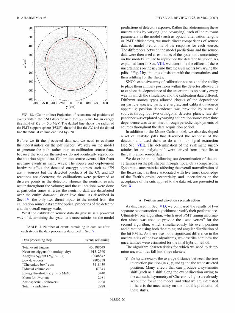
B. AHARMIM et al. PHYSICAL REVIEW C 75, 045502 (2007)
FIG. 18. (Color online) Projection of reconstructed positions ofevents within the SNO detector onto the z-y plane for an energythreshold of Teff > 5.0 MeV. The dashed line shows the radius ofthe PMT support sphere (PSUP), the solid line the AV, and the dottedline the fiducial volume cut used by SNO.
Before we fit the processed data set, we need to evaluatethe uncertainties on the pdf shapes. We rely on the modelto generate the pdfs, rather than on calibration source data,because the sources themselves do not identically reproducethe neutrino-signal data. Calibration source events differ fromneutrino events in many ways: The source and deploymenthardware affect the detected energy; sources such as 16Nare γ sources but the detected products of the CC and ESreactions are electrons; the calibrations were performed atdiscrete points in the detector, whereas the neutrino eventsoccur throughout the volume; and the calibrations were doneat particular times whereas the neutrino data are distributedover the entire data-acquisition live time. As described inSec. IV, the only two direct inputs to the model from thecalibration source data are the optical properties of the detectorand the overall energy scale.
What the calibration source data do give us is a powerfulway of determining the systematic uncertainties on the model
TABLE II. Number of events remaining in data set aftereach step in the data processing described in Sec. V.
Data processing step Events remaining
Total event triggers 450188649Neutrino triggers (hit multiplicity) 191312560Analysis Nhit cut (Nhit > 21) 10088842Low-level cuts 7805238“Cherenkov box” cuts 3418439Fiducial volume cut 67343Energy threshold (Teff > 5 MeV) 3440Muon follower cut 2981Atmospheric ν followers 2928Total ν candidates 2928
predictions of detector response. Rather than determining theseuncertainties by varying (and covarying) each of the relevantparameters in the model (such as optical attenuation lengthsor PMT efficiencies), we made direct comparisons of sourcedata to model predictions of the response for each source.The differences between the model predictions and the sourcedata were then used as estimates of the systematic uncertaintyon the model’s ability to reproduce the detector behavior. Asexplained later in Sec. VIII, we determine the effects of theseuncertainties on the neutrino flux measurements by varying thepdfs of Fig. 2 by amounts consistent with the uncertainties, andthen refitting for the fluxes.
SNO’s extensive array of calibration sources and the abilityto place them at many positions within the detector allowed usto explore the dependence of the uncertainties on nearly everyway in which the simulation and the calibration data differed.Different source types allowed checks of the dependenceon particle species, particle energies, and calibration-sourceapparatus; position dependence was provided by scans ofsources throughout two orthogonal detector planes; rate de-pendence was explored by varying calibration source rate; timedependence was determined through periodic deployments ofsources throughout the data acquisition period.
In addition to the Monte Carlo model, we also developeda set of analytic pdfs that described the response of thedetector and used them to do a similar signal extraction(see Sec. VIII). The determination of the systematic uncer-tainties for the analytic pdfs were derived from direct fits tothe calibration source data.
We describe in the following our determination of the un-certainties on the pdf shapes through model-data comparisons.Systematic uncertainties affecting the overall normalization ofthe fluxes such as those associated with live time, knowledgeof the Earth’s orbital eccentricity, and uncertainties on theacceptance of the cuts applied to the data set, are presented inSec. X.
A. Position and direction reconstruction
As discussed in Sec. V D, we compared the results of twoseparate reconstruction algorithms to verify their performance.Ultimately, one algorithm, which used PMT timing informa-tion alone, was used to provide the “seed vertex” for thesecond algorithm, which simultaneously fits event positionand direction using both the timing and angular distribution ofthe hit PMTs. As there was not a significant difference in theuncertainties of the two algorithms, we describe here how theuncertainties were estimated for the final hybrid method.
The algorithm characteristics for which we need to deter-mine uncertainties fall into three classes:
(i) Vertex accuracy: the average distance between the trueinteraction position (in x, y, and z) and the reconstructedposition. Many effects that can produce a systematicshift (such as a shift along the event direction owing tothe azimuthal symmetry of Cherenkov light) are alreadyaccounted for in the model, and what we are interestedin here is the uncertainty on the model’s prediction ofthese shifts.
045502-20
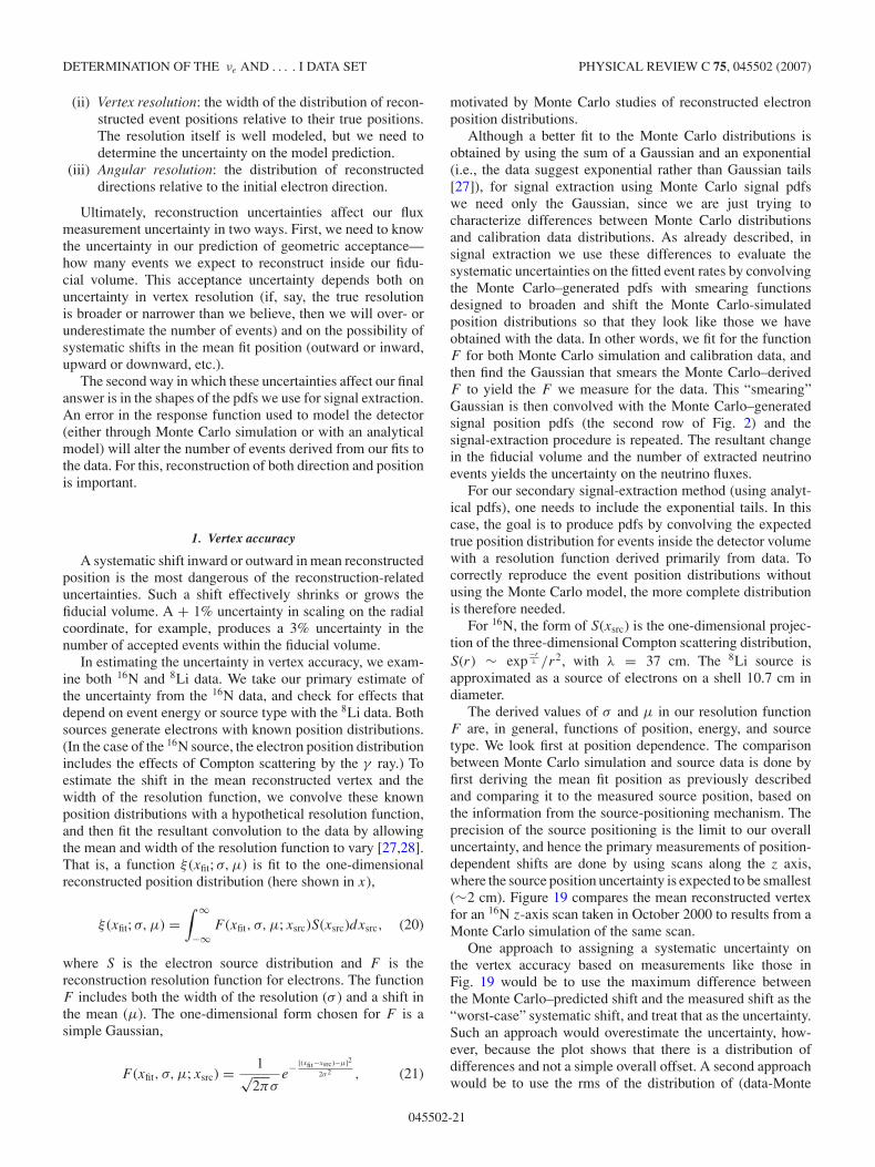
DETERMINATION OF THE νe AND . . . . I DATA SET PHYSICAL REVIEW C 75, 045502 (2007)
(ii) Vertex resolution: the width of the distribution of recon-structed event positions relative to their true positions.The resolution itself is well modeled, but we need todetermine the uncertainty on the model prediction.
(iii) Angular resolution: the distribution of reconstructeddirections relative to the initial electron direction.
Ultimately, reconstruction uncertainties affect our fluxmeasurement uncertainty in two ways. First, we need to knowthe uncertainty in our prediction of geometric acceptance—how many events we expect to reconstruct inside our fidu-cial volume. This acceptance uncertainty depends both onuncertainty in vertex resolution (if, say, the true resolutionis broader or narrower than we believe, then we will over- orunderestimate the number of events) and on the possibility ofsystematic shifts in the mean fit position (outward or inward,upward or downward, etc.).
The second way in which these uncertainties affect our finalanswer is in the shapes of the pdfs we use for signal extraction.An error in the response function used to model the detector(either through Monte Carlo simulation or with an analyticalmodel) will alter the number of events derived from our fits tothe data. For this, reconstruction of both direction and positionis important.
1. Vertex accuracy
A systematic shift inward or outward in mean reconstructedposition is the most dangerous of the reconstruction-relateduncertainties. Such a shift effectively shrinks or grows thefiducial volume. A + 1% uncertainty in scaling on the radialcoordinate, for example, produces a 3% uncertainty in thenumber of accepted events within the fiducial volume.
In estimating the uncertainty in vertex accuracy, we exam-ine both 16N and 8Li data. We take our primary estimate ofthe uncertainty from the 16N data, and check for effects thatdepend on event energy or source type with the 8Li data. Bothsources generate electrons with known position distributions.(In the case of the 16N source, the electron position distributionincludes the effects of Compton scattering by the γ ray.) Toestimate the shift in the mean reconstructed vertex and thewidth of the resolution function, we convolve these knownposition distributions with a hypothetical resolution function,and then fit the resultant convolution to the data by allowingthe mean and width of the resolution function to vary [27,28].That is, a function ξ (xfit; σ,µ) is fit to the one-dimensionalreconstructed position distribution (here shown in x),
ξ (xfit; σ,µ) =∫ ∞
−∞F (xfit, σ, µ; xsrc)S(xsrc)dxsrc, (20)
where S is the electron source distribution and F is thereconstruction resolution function for electrons. The functionF includes both the width of the resolution (σ ) and a shift inthe mean (µ). The one-dimensional form chosen for F is asimple Gaussian,
F (xfit, σ, µ; xsrc) = 1√2πσ
e− [(xfit−xsrc)−µ]2
2σ2 , (21)
motivated by Monte Carlo studies of reconstructed electronposition distributions.
Although a better fit to the Monte Carlo distributions isobtained by using the sum of a Gaussian and an exponential(i.e., the data suggest exponential rather than Gaussian tails[27]), for signal extraction using Monte Carlo signal pdfswe need only the Gaussian, since we are just trying tocharacterize differences between Monte Carlo distributionsand calibration data distributions. As already described, insignal extraction we use these differences to evaluate thesystematic uncertainties on the fitted event rates by convolvingthe Monte Carlo–generated pdfs with smearing functionsdesigned to broaden and shift the Monte Carlo-simulatedposition distributions so that they look like those we haveobtained with the data. In other words, we fit for the functionF for both Monte Carlo simulation and calibration data, andthen find the Gaussian that smears the Monte Carlo–derivedF to yield the F we measure for the data. This “smearing”Gaussian is then convolved with the Monte Carlo–generatedsignal position pdfs (the second row of Fig. 2) and thesignal-extraction procedure is repeated. The resultant changein the fiducial volume and the number of extracted neutrinoevents yields the uncertainty on the neutrino fluxes.
For our secondary signal-extraction method (using analyt-ical pdfs), one needs to include the exponential tails. In thiscase, the goal is to produce pdfs by convolving the expectedtrue position distribution for events inside the detector volumewith a resolution function derived primarily from data. Tocorrectly reproduce the event position distributions withoutusing the Monte Carlo model, the more complete distributionis therefore needed.
For 16N, the form of S(xsrc) is the one-dimensional projec-tion of the three-dimensional Compton scattering distribution,S(r) ∼ exp
−rλ /r2, with λ = 37 cm. The 8Li source is
approximated as a source of electrons on a shell 10.7 cm indiameter.
The derived values of σ and µ in our resolution functionF are, in general, functions of position, energy, and sourcetype. We look first at position dependence. The comparisonbetween Monte Carlo simulation and source data is done byfirst deriving the mean fit position as previously describedand comparing it to the measured source position, based onthe information from the source-positioning mechanism. Theprecision of the source positioning is the limit to our overalluncertainty, and hence the primary measurements of position-dependent shifts are done by using scans along the z axis,where the source position uncertainty is expected to be smallest(∼2 cm). Figure 19 compares the mean reconstructed vertexfor an 16N z-axis scan taken in October 2000 to results from aMonte Carlo simulation of the same scan.
One approach to assigning a systematic uncertainty onthe vertex accuracy based on measurements like those inFig. 19 would be to use the maximum difference betweenthe Monte Carlo–predicted shift and the measured shift as the“worst-case” systematic shift, and treat that as the uncertainty.Such an approach would overestimate the uncertainty, how-ever, because the plot shows that there is a distribution ofdifferences and not a simple overall offset. A second approachwould be to use the rms of the distribution of (data-Monte
045502-21
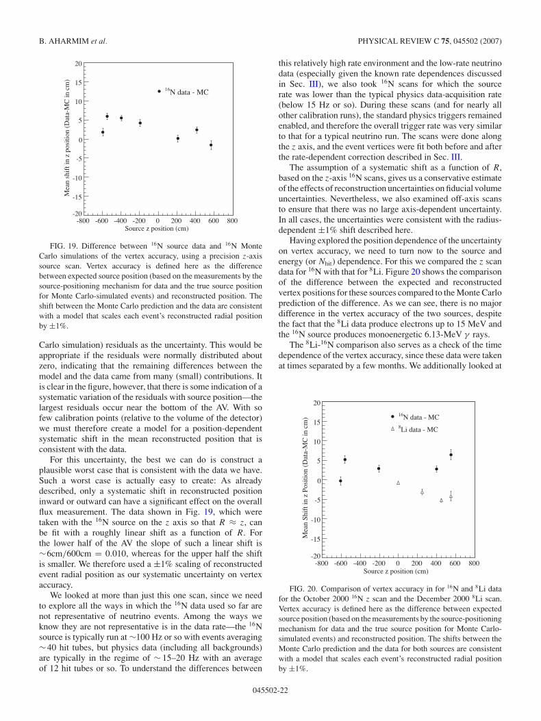
B. AHARMIM et al. PHYSICAL REVIEW C 75, 045502 (2007)
Source z position (cm)-800 -600 -400 -200 0 200 400 600 800
Mea
n sh
ift i
n z
posi
tion
(Dat
a-M
C in
cm
)
-20
-15
-10
-5
0
5
10
15
20
N data - MC16
FIG. 19. Difference between 16N source data and 16N MonteCarlo simulations of the vertex accuracy, using a precision z-axissource scan. Vertex accuracy is defined here as the differencebetween expected source position (based on the measurements by thesource-positioning mechanism for data and the true source positionfor Monte Carlo-simulated events) and reconstructed position. Theshift between the Monte Carlo prediction and the data are consistentwith a model that scales each event’s reconstructed radial positionby ±1%.
Carlo simulation) residuals as the uncertainty. This would beappropriate if the residuals were normally distributed aboutzero, indicating that the remaining differences between themodel and the data came from many (small) contributions. Itis clear in the figure, however, that there is some indication of asystematic variation of the residuals with source position—thelargest residuals occur near the bottom of the AV. With sofew calibration points (relative to the volume of the detector)we must therefore create a model for a position-dependentsystematic shift in the mean reconstructed position that isconsistent with the data.
For this uncertainty, the best we can do is construct aplausible worst case that is consistent with the data we have.Such a worst case is actually easy to create: As alreadydescribed, only a systematic shift in reconstructed positioninward or outward can have a significant effect on the overallflux measurement. The data shown in Fig. 19, which weretaken with the 16N source on the z axis so that R ≈ z, canbe fit with a roughly linear shift as a function of R. Forthe lower half of the AV the slope of such a linear shift is∼6cm/600cm = 0.010, whereas for the upper half the shiftis smaller. We therefore used a ±1% scaling of reconstructedevent radial position as our systematic uncertainty on vertexaccuracy.
We looked at more than just this one scan, since we needto explore all the ways in which the 16N data used so far arenot representative of neutrino events. Among the ways weknow they are not representative is in the data rate—the 16Nsource is typically run at ∼100 Hz or so with events averaging∼40 hit tubes, but physics data (including all backgrounds)are typically in the regime of ∼ 15–20 Hz with an averageof 12 hit tubes or so. To understand the differences between
this relatively high rate environment and the low-rate neutrinodata (especially given the known rate dependences discussedin Sec. III), we also took 16N scans for which the sourcerate was lower than the typical physics data-acquisition rate(below 15 Hz or so). During these scans (and for nearly allother calibration runs), the standard physics triggers remainedenabled, and therefore the overall trigger rate was very similarto that for a typical neutrino run. The scans were done alongthe z axis, and the event vertices were fit both before and afterthe rate-dependent correction described in Sec. III.
The assumption of a systematic shift as a function of R,based on the z-axis 16N scans, gives us a conservative estimateof the effects of reconstruction uncertainties on fiducial volumeuncertainties. Nevertheless, we also examined off-axis scansto ensure that there was no large axis-dependent uncertainty.In all cases, the uncertainties were consistent with the radius-dependent ±1% shift described here.
Having explored the position dependence of the uncertaintyon vertex accuracy, we need to turn now to the source andenergy (or Nhit) dependence. For this we compared the z scandata for 16N with that for 8Li. Figure 20 shows the comparisonof the difference between the expected and reconstructedvertex positions for these sources compared to the Monte Carloprediction of the difference. As we can see, there is no majordifference in the vertex accuracy of the two sources, despitethe fact that the 8Li data produce electrons up to 15 MeV andthe 16N source produces monoenergetic 6.13-MeV γ rays.
The 8Li-16N comparison also serves as a check of the timedependence of the vertex accuracy, since these data were takenat times separated by a few months. We additionally looked at
Source z position (cm)-800 -600 -400 -200 0 200 400 600 800
Mea
n Sh
ift i
n z
Posi
tion
(Dat
a-M
C in
cm
)
-20
-15
-10
-5
0
5
10
15
20
N data - MC16
Li data - MC8
FIG. 20. Comparison of vertex accuracy in for 16N and 8Li datafor the October 2000 16N z scan and the December 2000 8Li scan.Vertex accuracy is defined here as the difference between expectedsource position (based on the measurements by the source-positioningmechanism for data and the true source position for Monte Carlo-simulated events) and reconstructed position. The shifts between theMonte Carlo prediction and the data for both sources are consistentwith a model that scales each event’s reconstructed radial positionby ±1%.
045502-22
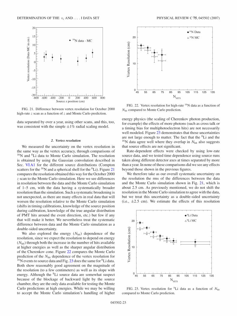
DETERMINATION OF THE νe AND . . . . I DATA SET PHYSICAL REVIEW C 75, 045502 (2007)
Source z position (cm)-800 -600 -400 -200 0 200 400 600 800
Ver
tex
reso
lutio
n (D
ata-
MC
in c
m)
-20
-15
-10
-5
0
5
10
15
20
N data - MC16
FIG. 21. Difference between vertex resolution for October 2000high-rate z scan as a function of z and Monte Carlo prediction.
data separated by over a year, using other scans, and this, too,was consistent with the simple ±1% radial scaling model.
2. Vertex resolution
We measured the uncertainty on the vertex resolution inthe same way as the vertex accuracy, through comparisons of16N and 8Li data to Monte Carlo simulation. The resolutionis obtained by using the Gaussian convolution described inSec. VI A1 for the different source distributions (Comptonscatters for the 16N and a spherical shell for the 8Li). Figure 21compares the resolution obtained this way for the October 2000z scan to the Monte Carlo simulation. Here we see differencesin resolution between the data and the Monte Carlo simulationof 1–5 cm, with the data having a systematically broaderresolution than the simulation. Such a systematic broadening isnot unexpected, as there are many effects in real data that willworsen the resolution relative to the Monte Carlo simulation(shifts in timing calibrations, knowledge of the source positionduring calibration, knowledge of the true angular distributionof PMT hits around the event direction, etc.) but few if anythat will make it better. We nevertheless treat the systematicdifference between data and the Monte Carlo simulation as adouble-sided uncertainty.
We also explored the energy (Nhit) dependence of theresolution, since we expect the resolution to depend on energy(Nhit) through both the increase in the number of hits availableat higher energies as well as the sharper angular distributionof the Cherenkov cone. Figure 22 compares the Monte Carloprediction of the Nhit dependence of the vertex resolution for16N events to source data and Fig. 23 does the same for 8Li data.Both show reasonably good agreement on the magnitude ofthe resolution (to a few centimeters) as well as its slope withenergy. Although the 8Li source data are somewhat suspectbecause of the blockage of backward light by the sourcechamber, they are the only data available for testing the MonteCarlo predictions at high energies. While we may be willingto accept the Monte Carlo simulation’s handling of higher
16
16
HITS
FIG. 22. Vertex resolution for high-rate 16N data as a function ofNhit compared to Monte Carlo prediction.
energy physics (the scaling of Cherenkov photon production,for example) the effects of more photons (such as cross talk ora timing bias for multiphotoelectron hits) are not necessarilywell modeled. Figure 23 demonstrates that those uncertaintiesare not large enough to matter. The fact that the 8Li and the16N data agree well where they overlap in Nhit also suggeststhat source effects are not significant.
Rate-dependent effects were checked by using low-ratesource data, and we tested time dependence using source runstaken along different detector axes at times separated by morethan a year. In none of these comparisons did we see any effectsbeyond those shown in the previous figures.
We therefore take as our overall systematic uncertainty onthe resolution the rms of the differences between the dataand the Monte Carlo simulation shown in Fig. 21, which isabout 2.5 cm. As previously mentioned, we do not shift theresolution in the Monte Carlo simulation to agree with the data,but we treat this uncertainty as a double-sided uncertainty(i.e., ±2.5 cm). We estimate the effects of this resolution
8
HITS
8
FIG. 23. Vertex resolution for 8Li data as a function of Nhit
compared to Monte Carlo prediction.
045502-23
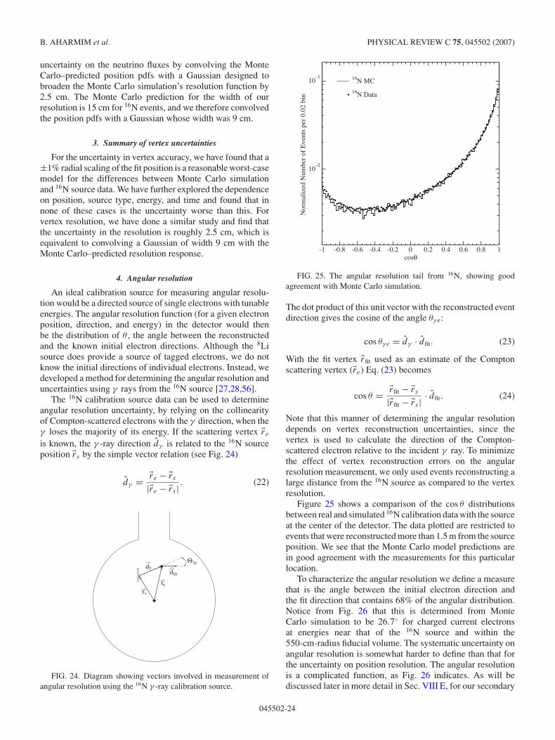
B. AHARMIM et al. PHYSICAL REVIEW C 75, 045502 (2007)
uncertainty on the neutrino fluxes by convolving the MonteCarlo–predicted position pdfs with a Gaussian designed tobroaden the Monte Carlo simulation’s resolution function by2.5 cm. The Monte Carlo prediction for the width of ourresolution is 15 cm for 16N events, and we therefore convolvedthe position pdfs with a Gaussian whose width was 9 cm.
3. Summary of vertex uncertainties
For the uncertainty in vertex accuracy, we have found that a±1% radial scaling of the fit position is a reasonable worst-casemodel for the differences between Monte Carlo simulationand 16N source data. We have further explored the dependenceon position, source type, energy, and time and found that innone of these cases is the uncertainty worse than this. Forvertex resolution, we have done a similar study and find thatthe uncertainty in the resolution is roughly 2.5 cm, which isequivalent to convolving a Gaussian of width 9 cm with theMonte Carlo–predicted resolution response.
4. Angular resolution
An ideal calibration source for measuring angular resolu-tion would be a directed source of single electrons with tunableenergies. The angular resolution function (for a given electronposition, direction, and energy) in the detector would thenbe the distribution of θ , the angle between the reconstructedand the known initial electron directions. Although the 8Lisource does provide a source of tagged electrons, we do notknow the initial directions of individual electrons. Instead, wedeveloped a method for determining the angular resolution anduncertainties using γ rays from the 16N source [27,28,56].
The 16N calibration source data can be used to determineangular resolution uncertainty, by relying on the collinearityof Compton-scattered electrons with the γ direction, when theγ loses the majority of its energy. If the scattering vertex re
is known, the γ -ray direction dγ is related to the 16N sourceposition rs by the simple vector relation (see Fig. 24)
dγ = re − rs
|re − rs | . (22)
rr
dd
e
s
γfit
Θγe
FIG. 24. Diagram showing vectors involved in measurement ofangular resolution using the 16N γ -ray calibration source.
16N MC
16N Data
cosθ
Nor
mal
ized
Num
ber
of E
vent
s pe
r 0.
02 b
in
10-2
10-1
-1 -0.8 -0.6 -0.4 -0.2 0 0.2 0.4 0.6 0.8 1
FIG. 25. The angular resolution tail from 16N, showing goodagreement with Monte Carlo simulation.
The dot product of this unit vector with the reconstructed eventdirection gives the cosine of the angle θγ e:
cos θγ e = dγ · dfit. (23)
With the fit vertex rfit used as an estimate of the Comptonscattering vertex (re) Eq. (23) becomes
cos θ = rfit − rs
|rfit − rs | · dfit. (24)
Note that this manner of determining the angular resolutiondepends on vertex reconstruction uncertainties, since thevertex is used to calculate the direction of the Compton-scattered electron relative to the incident γ ray. To minimizethe effect of vertex reconstruction errors on the angularresolution measurement, we only used events reconstructing alarge distance from the 16N source as compared to the vertexresolution.
Figure 25 shows a comparison of the cos θ distributionsbetween real and simulated 16N calibration data with the sourceat the center of the detector. The data plotted are restricted toevents that were reconstructed more than 1.5 m from the sourceposition. We see that the Monte Carlo model predictions arein good agreement with the measurements for this particularlocation.
To characterize the angular resolution we define a measurethat is the angle between the initial electron direction andthe fit direction that contains 68% of the angular distribution.Notice from Fig. 26 that this is determined from MonteCarlo simulation to be 26.7◦ for charged current electronsat energies near that of the 16N source and within the550-cm-radius fiducial volume. The systematic uncertainty onangular resolution is somewhat harder to define than that forthe uncertainty on position resolution. The angular resolutionis a complicated function, as Fig. 26 indicates. As will bediscussed later in more detail in Sec. VIII E, for our secondary
045502-24
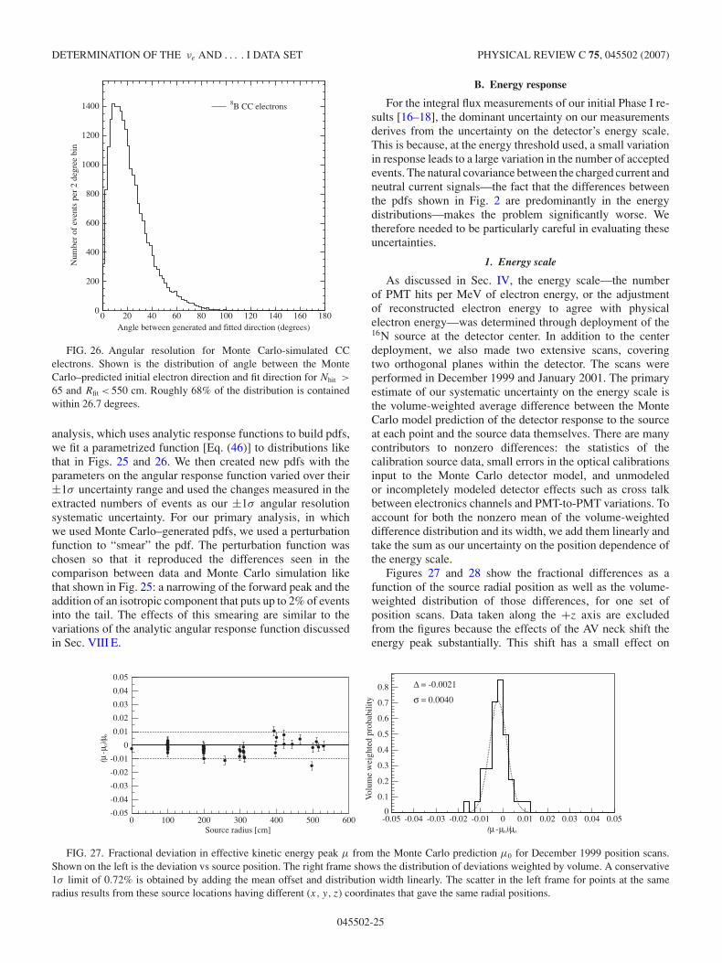
DETERMINATION OF THE νe AND . . . . I DATA SET PHYSICAL REVIEW C 75, 045502 (2007)
8B CC electrons
Angle between generated and fitted direction (degrees)
Num
ber
of e
vent
s pe
r 2
degr
ee b
in
0
200
400
600
800
1000
1200
1400
0 20 40 60 80 100 120 140 160 180
FIG. 26. Angular resolution for Monte Carlo-simulated CCelectrons. Shown is the distribution of angle between the MonteCarlo–predicted initial electron direction and fit direction for Nhit >
65 and Rfit < 550 cm. Roughly 68% of the distribution is containedwithin 26.7 degrees.
analysis, which uses analytic response functions to build pdfs,we fit a parametrized function [Eq. (46)] to distributions likethat in Figs. 25 and 26. We then created new pdfs with theparameters on the angular response function varied over their±1σ uncertainty range and used the changes measured in theextracted numbers of events as our ±1σ angular resolutionsystematic uncertainty. For our primary analysis, in whichwe used Monte Carlo–generated pdfs, we used a perturbationfunction to “smear” the pdf. The perturbation function waschosen so that it reproduced the differences seen in thecomparison between data and Monte Carlo simulation likethat shown in Fig. 25: a narrowing of the forward peak and theaddition of an isotropic component that puts up to 2% of eventsinto the tail. The effects of this smearing are similar to thevariations of the analytic angular response function discussedin Sec. VIII E.
B. Energy response
For the integral flux measurements of our initial Phase I re-sults [16–18], the dominant uncertainty on our measurementsderives from the uncertainty on the detector’s energy scale.This is because, at the energy threshold used, a small variationin response leads to a large variation in the number of acceptedevents. The natural covariance between the charged current andneutral current signals—the fact that the differences betweenthe pdfs shown in Fig. 2 are predominantly in the energydistributions—makes the problem significantly worse. Wetherefore needed to be particularly careful in evaluating theseuncertainties.
1. Energy scale
As discussed in Sec. IV, the energy scale—the numberof PMT hits per MeV of electron energy, or the adjustmentof reconstructed electron energy to agree with physicalelectron energy—was determined through deployment of the16N source at the detector center. In addition to the centerdeployment, we also made two extensive scans, coveringtwo orthogonal planes within the detector. The scans wereperformed in December 1999 and January 2001. The primaryestimate of our systematic uncertainty on the energy scale isthe volume-weighted average difference between the MonteCarlo model prediction of the detector response to the sourceat each point and the source data themselves. There are manycontributors to nonzero differences: the statistics of thecalibration source data, small errors in the optical calibrationsinput to the Monte Carlo detector model, and unmodeledor incompletely modeled detector effects such as cross talkbetween electronics channels and PMT-to-PMT variations. Toaccount for both the nonzero mean of the volume-weighteddifference distribution and its width, we add them linearly andtake the sum as our uncertainty on the position dependence ofthe energy scale.
Figures 27 and 28 show the fractional differences as afunction of the source radial position as well as the volume-weighted distribution of those differences, for one set ofposition scans. Data taken along the +z axis are excludedfrom the figures because the effects of the AV neck shift theenergy peak substantially. This shift has a small effect on
oµ)/oµ - µ(-0.05 -0.04 -0.03 -0.02 -0.01 0 0.01 0.02 0.03 0.04 0.05
Vol
ume
wei
ghte
d pr
obab
ility
0
0.1
0.2
0.3
0.4
0.5
0.6
0.7
0.8 = -0.0021 ∆
= 0.0040 σ
Source radius [cm]0 100 200 300 400 500 600
oµ)/ oµ -
µ(
-0.05
-0.04
-0.03
-0.02
-0.01
0
0.01
0.02
0.03
0.04
0.05
FIG. 27. Fractional deviation in effective kinetic energy peak µ from the Monte Carlo prediction µ0 for December 1999 position scans.Shown on the left is the deviation vs source position. The right frame shows the distribution of deviations weighted by volume. A conservative1σ limit of 0.72% is obtained by adding the mean offset and distribution width linearly. The scatter in the left frame for points at the sameradius results from these source locations having different (x, y, z) coordinates that gave the same radial positions.
045502-25
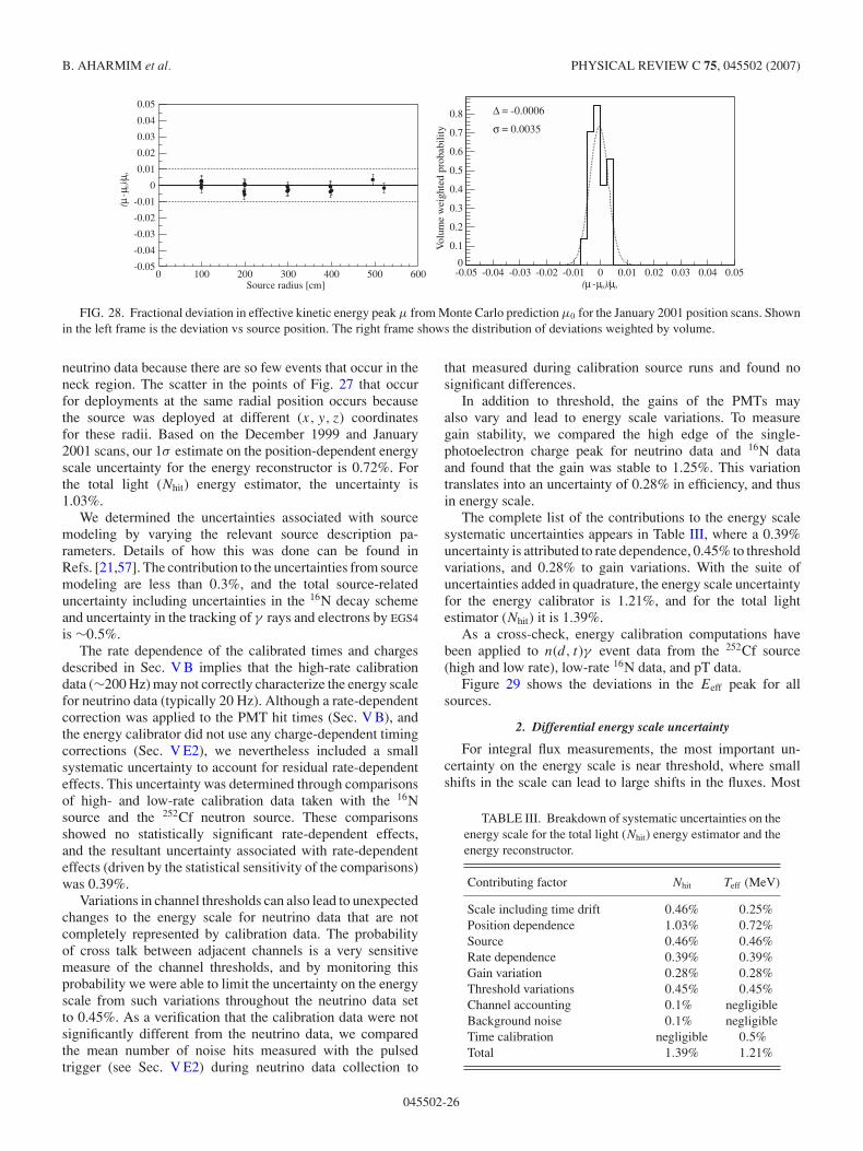
B. AHARMIM et al. PHYSICAL REVIEW C 75, 045502 (2007)
oµ)/oµ - µ(-0.05 -0.04 -0.03 -0.02 -0.01 0 0.01 0.02 0.03 0.04 0.05
Vol
ume
wei
ghte
d pr
obab
ility
0
0.1
0.2
0.3
0.4
0.5
0.6
0.7
0.8 = -0.0006 ∆
= 0.0035 σ
Source radius [cm]0 100 200 300 400 500 600
oµ)/ oµ -
µ(
-0.05
-0.04
-0.03
-0.02
-0.01
0
0.01
0.02
0.03
0.04
0.05
FIG. 28. Fractional deviation in effective kinetic energy peak µ from Monte Carlo prediction µ0 for the January 2001 position scans. Shownin the left frame is the deviation vs source position. The right frame shows the distribution of deviations weighted by volume.
neutrino data because there are so few events that occur in theneck region. The scatter in the points of Fig. 27 that occurfor deployments at the same radial position occurs becausethe source was deployed at different (x, y, z) coordinatesfor these radii. Based on the December 1999 and January2001 scans, our 1σ estimate on the position-dependent energyscale uncertainty for the energy reconstructor is 0.72%. Forthe total light (Nhit) energy estimator, the uncertainty is1.03%.
We determined the uncertainties associated with sourcemodeling by varying the relevant source description pa-rameters. Details of how this was done can be found inRefs. [21,57]. The contribution to the uncertainties from sourcemodeling are less than 0.3%, and the total source-relateduncertainty including uncertainties in the 16N decay schemeand uncertainty in the tracking of γ rays and electrons by EGS4
is ∼0.5%.The rate dependence of the calibrated times and charges
described in Sec. V B implies that the high-rate calibrationdata (∼200 Hz) may not correctly characterize the energy scalefor neutrino data (typically 20 Hz). Although a rate-dependentcorrection was applied to the PMT hit times (Sec. V B), andthe energy calibrator did not use any charge-dependent timingcorrections (Sec. V E2), we nevertheless included a smallsystematic uncertainty to account for residual rate-dependenteffects. This uncertainty was determined through comparisonsof high- and low-rate calibration data taken with the 16Nsource and the 252Cf neutron source. These comparisonsshowed no statistically significant rate-dependent effects,and the resultant uncertainty associated with rate-dependenteffects (driven by the statistical sensitivity of the comparisons)was 0.39%.
Variations in channel thresholds can also lead to unexpectedchanges to the energy scale for neutrino data that are notcompletely represented by calibration data. The probabilityof cross talk between adjacent channels is a very sensitivemeasure of the channel thresholds, and by monitoring thisprobability we were able to limit the uncertainty on the energyscale from such variations throughout the neutrino data setto 0.45%. As a verification that the calibration data were notsignificantly different from the neutrino data, we comparedthe mean number of noise hits measured with the pulsedtrigger (see Sec. V E2) during neutrino data collection to
that measured during calibration source runs and found nosignificant differences.
In addition to threshold, the gains of the PMTs mayalso vary and lead to energy scale variations. To measuregain stability, we compared the high edge of the single-photoelectron charge peak for neutrino data and 16N dataand found that the gain was stable to 1.25%. This variationtranslates into an uncertainty of 0.28% in efficiency, and thusin energy scale.
The complete list of the contributions to the energy scalesystematic uncertainties appears in Table III, where a 0.39%uncertainty is attributed to rate dependence, 0.45% to thresholdvariations, and 0.28% to gain variations. With the suite ofuncertainties added in quadrature, the energy scale uncertaintyfor the energy calibrator is 1.21%, and for the total lightestimator (Nhit) it is 1.39%.
As a cross-check, energy calibration computations havebeen applied to n(d, t)γ event data from the 252Cf source(high and low rate), low-rate 16N data, and pT data.
Figure 29 shows the deviations in the Eeff peak for allsources.
2. Differential energy scale uncertainty
For integral flux measurements, the most important un-certainty on the energy scale is near threshold, where smallshifts in the scale can lead to large shifts in the fluxes. Most
TABLE III. Breakdown of systematic uncertainties on theenergy scale for the total light (Nhit) energy estimator and theenergy reconstructor.
Contributing factor Nhit Teff (MeV)
Scale including time drift 0.46% 0.25%Position dependence 1.03% 0.72%Source 0.46% 0.46%Rate dependence 0.39% 0.39%Gain variation 0.28% 0.28%Threshold variations 0.45% 0.45%Channel accounting 0.1% negligibleBackground noise 0.1% negligibleTime calibration negligible 0.5%Total 1.39% 1.21%
045502-26
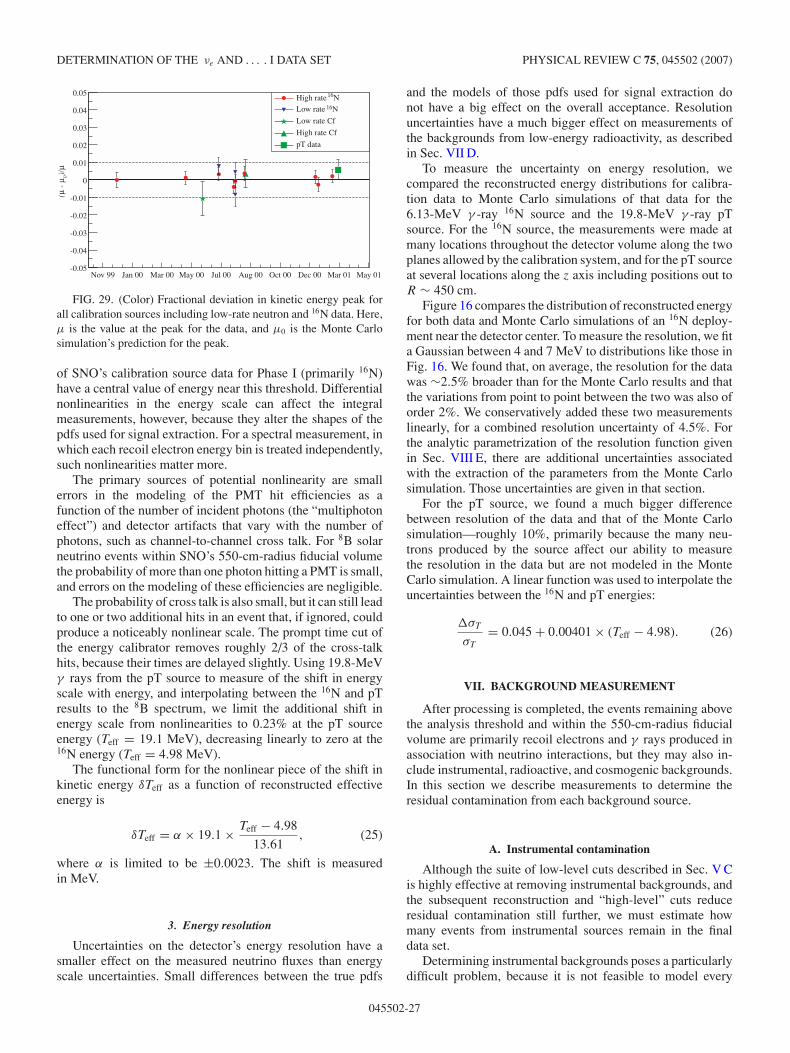
DETERMINATION OF THE νe AND . . . . I DATA SET PHYSICAL REVIEW C 75, 045502 (2007)
Nov 99 Jan 00 Mar 00 May 00 Jul 00 Aug 00 Oct 00 Dec 00 Mar 01 May 01
µ)/
0µ -
µ(
-0.05
-0.04
-0.03
-0.02
-0.01
0
0.01
0.02
0.03
0.04
0.05N16High rate N16Low rate
Low rate Cf
High rate Cf
pT data
FIG. 29. (Color) Fractional deviation in kinetic energy peak forall calibration sources including low-rate neutron and 16N data. Here,µ is the value at the peak for the data, and µ0 is the Monte Carlosimulation’s prediction for the peak.
of SNO’s calibration source data for Phase I (primarily 16N)have a central value of energy near this threshold. Differentialnonlinearities in the energy scale can affect the integralmeasurements, however, because they alter the shapes of thepdfs used for signal extraction. For a spectral measurement, inwhich each recoil electron energy bin is treated independently,such nonlinearities matter more.
The primary sources of potential nonlinearity are smallerrors in the modeling of the PMT hit efficiencies as afunction of the number of incident photons (the “multiphotoneffect”) and detector artifacts that vary with the number ofphotons, such as channel-to-channel cross talk. For 8B solarneutrino events within SNO’s 550-cm-radius fiducial volumethe probability of more than one photon hitting a PMT is small,and errors on the modeling of these efficiencies are negligible.
The probability of cross talk is also small, but it can still leadto one or two additional hits in an event that, if ignored, couldproduce a noticeably nonlinear scale. The prompt time cut ofthe energy calibrator removes roughly 2/3 of the cross-talkhits, because their times are delayed slightly. Using 19.8-MeVγ rays from the pT source to measure of the shift in energyscale with energy, and interpolating between the 16N and pTresults to the 8B spectrum, we limit the additional shift inenergy scale from nonlinearities to 0.23% at the pT sourceenergy (Teff = 19.1 MeV), decreasing linearly to zero at the16N energy (Teff = 4.98 MeV).
The functional form for the nonlinear piece of the shift inkinetic energy δTeff as a function of reconstructed effectiveenergy is
δTeff = α × 19.1 × Teff − 4.98
13.61, (25)
where α is limited to be ±0.0023. The shift is measuredin MeV.
3. Energy resolution
Uncertainties on the detector’s energy resolution have asmaller effect on the measured neutrino fluxes than energyscale uncertainties. Small differences between the true pdfs
and the models of those pdfs used for signal extraction donot have a big effect on the overall acceptance. Resolutionuncertainties have a much bigger effect on measurements ofthe backgrounds from low-energy radioactivity, as describedin Sec. VII D.
To measure the uncertainty on energy resolution, wecompared the reconstructed energy distributions for calibra-tion data to Monte Carlo simulations of that data for the6.13-MeV γ -ray 16N source and the 19.8-MeV γ -ray pTsource. For the 16N source, the measurements were made atmany locations throughout the detector volume along the twoplanes allowed by the calibration system, and for the pT sourceat several locations along the z axis including positions out toR ∼ 450 cm.
Figure 16 compares the distribution of reconstructed energyfor both data and Monte Carlo simulations of an 16N deploy-ment near the detector center. To measure the resolution, we fita Gaussian between 4 and 7 MeV to distributions like those inFig. 16. We found that, on average, the resolution for the datawas ∼2.5% broader than for the Monte Carlo results and thatthe variations from point to point between the two was also oforder 2%. We conservatively added these two measurementslinearly, for a combined resolution uncertainty of 4.5%. Forthe analytic parametrization of the resolution function givenin Sec. VIII E, there are additional uncertainties associatedwith the extraction of the parameters from the Monte Carlosimulation. Those uncertainties are given in that section.
For the pT source, we found a much bigger differencebetween resolution of the data and that of the Monte Carlosimulation—roughly 10%, primarily because the many neu-trons produced by the source affect our ability to measurethe resolution in the data but are not modeled in the MonteCarlo simulation. A linear function was used to interpolate theuncertainties between the 16N and pT energies:
�σT
σT
= 0.045 + 0.00401 × (Teff − 4.98). (26)
VII. BACKGROUND MEASUREMENT
After processing is completed, the events remaining abovethe analysis threshold and within the 550-cm-radius fiducialvolume are primarily recoil electrons and γ rays produced inassociation with neutrino interactions, but they may also in-clude instrumental, radioactive, and cosmogenic backgrounds.In this section we describe measurements to determine theresidual contamination from each background source.
A. Instrumental contamination
Although the suite of low-level cuts described in Sec. V Cis highly effective at removing instrumental backgrounds, andthe subsequent reconstruction and “high-level” cuts reduceresidual contamination still further, we must estimate howmany events from instrumental sources remain in the finaldata set.
Determining instrumental backgrounds poses a particularlydifficult problem, because it is not feasible to model every
045502-27
B. AHARMIM et al. PHYSICAL REVIEW C 75, 045502 (2007)
possible ill-understood non-Cherenkov background source.Instead, we need a method that can determine the backgroundlevel irrespective of its source. The method we adopted for thisanalysis combined the low-level cuts and the high-level cuts inwhat is sometimes referred to as a “bifurcated analysis” [58].For more detail than we give here, see Ref. [59].
In a bifurcated analysis one picks two cuts (or two sets ofcuts as we have done) and counts the numbers of events inthe data set rejected by either cut, both cuts, or neither cut.We assume that the data set consists of just two classes ofevents, signal events ν and background events β, so that thetotal number of events in the data set is just S = β + ν. Thebackground contamination in the final signal sample is justthe fraction of β that passes both sets of cuts. If the acceptancefor background events by cut set i is yi , the final backgroundcontamination is K = y1y2β. If the acceptance for signalevents by cut set i is xi , the final number of signal events isx1x2ν.
We start with three separate event totals: the number ofevents that pass both cuts (a), the number that fail cut 1 butpass cut 2 (b), and the number that pass cut 1 but fail cut 2 (c).We then relate all of these with a linear system of equations:
a + c = x1ν + y1β, (27)
a + b = x2ν + y2β, (28)
a = x1x2ν + y1y2β, (29)
β + ν = S, (30)
which we solve analytically to determine the remainingbackground contamination K = y1y2β. The values for thecut acceptances will be discussed later in Sec. IX C.
We illustrate the general approach in Fig. 17, which shows16N events events in blue, neutrino candidate events in gray,and instrumental background events in black on a “high-level”cut plot. The in-time ratio (ITR) is on the horizontal axis andthe average PMT pair angle θij is on the vertical axis. The 16Ndata define a “Cherenkov box” (see Sec. V F) that containsmost of the neutrino event candidates. Most instrumentalbackground events, defined as events that fail the “low-level”cuts, lie outside the Cherenkov box. Our bifurcated analysismeasures the ratio of the number of events failing the low-levelcuts that lie within the Cherenkov box to those that lie outside,and it also measures the number of events that pass thelow-level cuts but lie outside the Cherenkov box. The numberof background events within the Cherenkov box (i.e., that passboth the low-level and high-level cuts) is then the product ofthese two numbers. For the final Phase I data set, we findusing this technique that the overall contamination has a 95%confidence level upper limit of K � 3 events.
The dominant systematic uncertainties in this analysis arethe uncertainties on the cut acceptances (see Secs. IX C1 andIX C3) and the possibility of variations in the efficiency of thecuts for removing backgrounds. For the latter, we looked atthe stability of each cut as a function of time using calibrationsource data.
For this analysis to work, the two sets of cuts we usemust be orthogonal to one another—we must be sure thatthe probability of passing the low-level cuts does not increasethe probability of passing the high-level cuts. To demonstrate
orthogonality, we loosened the cuts (essentially opening thefinal “signal box” defined by those events that pass both sets ofcuts) and measured the increase in the number of backgroundevents. With the looser cuts, we found the increase in thenumber of background events agreed well with what would beexpected for orthogonal cuts.
To ensure that there were no instrumental backgroundsmissed by this analysis, we also examined many differentdistributions of events and hits in “detector coordinates”—thenumber of hits as a function of electronics channel (ratherthan PMT), the distribution of event directions relative tothe detector’s zenith (rather than the solar direction), and thegeneral PMT-by-PMT occupancy. We found no evidence ofany remaining non-Cherenkov-light background.
In addition, we repeated the bifurcated analysis usingdifferent sets of cuts—for example replacing the cut on themean PMT pair angle with a cut on an event “isotropy” pa-rameter derived from the full two-point PMT-PMT correlationfunction, or using only a subset of the low-level cut suite.All differences in the results were very small and within ourexpectations.
B. Photodisintegration background
By far the most dangerous background to the NC measure-ment are the neutrons produced through photodisintegrationof deuterons by low-energy radioactivity. In particular, 232Thand 238U have γ rays at the end of their decay chains (2.61and 2.44 MeV, respectively) that are above the 2.22-MeVdeuteron binding energy. Low levels of these nuclei can befound in all the components of the detector: the heavy water,the AV, the light water, PMT support structure, as well asthe PMT glass and base hardware. The neutrons produced byphotodisintegration are indistinguishable from those producedby the NC reaction, and therefore measurements of thebackground levels inside the detector are crucial for correctnormalization of the total 8B flux. It is critical to measure thelevels of 232Th and 238U separately as the fraction of decaysthat lead to γ rays above 2.2 MeV are very different (36% and2%, respectively). Additionally, the photodisintegration crosssection depends strongly on the decay-γ -ray energy.
The first step in dealing with these backgrounds was tobuild the detector with very stringent radiopurity targets forall components. Table IV lists the 232Th and 238U targetlevels for the D2O, AV, and H2O. (At these radiopuritylevels, the background to the NC signal is approximately 1neutron produced per day or ∼10% of the NC signal.) In thissection, we describe the techniques developed to measure the232Th and 238U concentrations in different detector regions
TABLE IV. The target radio-purity levels fordifferent components in the SNO detector.
Component 232Th (g/g) 238U (g/g)
D2O 3.7 × 10⁻¹⁵ 4.5 × 10⁻¹⁴
H2O 3.7 × 10⁻¹⁴ 4.5 × 10⁻¹³
AV 1.9 × 10⁻¹² 3.6 × 10⁻¹²
045502-28
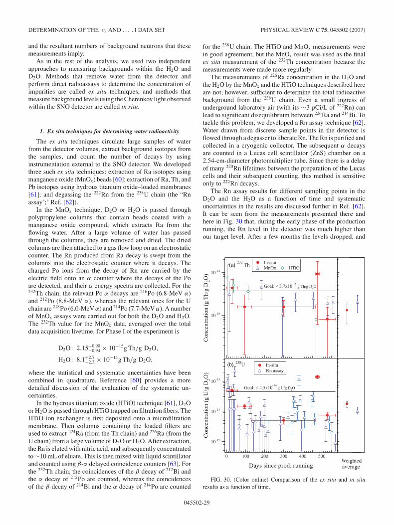
DETERMINATION OF THE νe AND . . . . I DATA SET PHYSICAL REVIEW C 75, 045502 (2007)
and the resultant numbers of background neutrons that thesemeasurements imply.
As in the rest of the analysis, we used two independentapproaches to measuring backgrounds within the H2O andD2O. Methods that remove water from the detector andperform direct radioassays to determine the concentration ofimpurities are called ex situ techniques, and methods thatmeasure background levels using the Cherenkov light observedwithin the SNO detector are called in situ.
1. Ex situ techniques for determining water radioactivity
The ex situ techniques circulate large samples of waterfrom the detector volumes, extract background isotopes fromthe samples, and count the number of decays by usinginstrumentation external to the SNO detector. We developedthree such ex situ techniques: extraction of Ra isotopes usingmanganese oxide (MnOx) beads [60]; extraction of Ra, Th, andPb isotopes using hydrous titanium oxide–loaded membranes[61]; and degassing the 222Rn from the 238U chain (the “Rnassay’;’ Ref. [62]).
In the MnOx technique, D2O or H2O is passed throughpolypropylene columns that contain beads coated with amanganese oxide compound, which extracts Ra from theflowing water. After a large volume of water has passedthrough the columns, they are removed and dried. The driedcolumns are then attached to a gas flow loop on an electrostaticcounter. The Rn produced from Ra decay is swept from thecolumns into the electrostatic counter where it decays. Thecharged Po ions from the decay of Rn are carried by theelectric field onto an α counter where the decays of the Poare detected, and their α energy spectra are collected. For the232Th chain, the relevant Po α decays are 216Po (6.8-MeV α)and 212Po (8.8-MeV α), whereas the relevant ones for the Uchain are 218Po (6.0-MeV α) and 214Po (7.7-MeV α). A numberof MnOx assays were carried out for both the D2O and H2O.The 232Th value for the MnOx data, averaged over the totaldata acquisition livetime, for Phase I of the experiment is
D2O: 2.15+0.90−0.94 × 10⁻¹⁵g Th/g D2O,
H2O: 8.1+2.7−2.3 × 10⁻¹⁴g Th/g D2O,
where the statistical and systematic uncertainties have beencombined in quadrature. Reference [60] provides a moredetailed discussion of the evaluation of the systematic un-certainties.
In the hydrous titanium oxide (HTiO) technique [61], D2Oor H2O is passed through HTiO trapped on filtration fibers. TheHTiO ion exchanger is first deposited onto a microfiltrationmembrane. Then columns containing the loaded filters areused to extract 224Ra (from the Th chain) and 226Ra (from theU chain) from a large volume of D2O or H2O. After extraction,the Ra is eluted with nitric acid, and subsequently concentratedto ∼10 mL of eluate. This is then mixed with liquid scintillatorand counted using β-α delayed coincidence counters [63]. Forthe 232Th chain, the coincidences of the β decay of 212Bi andthe α decay of 212Po are counted, whereas the coincidencesof the β decay of 214Bi and the α decay of 214Po are counted
for the 238U chain. The HTiO and MnOx measurements werein good agreement, but the MnOx result was used as the finalex situ measurement of the 232Th concentration because themeasurements were made more regularly.
The measurements of 226Ra concentration in the D2O andthe H2O by the MnOx and the HTiO techniques described hereare not, however, sufficient to determine the total radioactivebackground from the 238U chain. Even a small ingress ofunderground laboratory air (with its ∼3 pCi/L of 222Rn) canlead to significant disequilibrium between 226Ra and 214Bi. Totackle this problem, we developed a Rn assay technique [62].Water drawn from discrete sample points in the detector isflowed through a degasser to liberate Rn. The Rn is purified andcollected in a cryogenic collector. The subsequent α decaysare counted in a Lucas cell scintillator (ZnS) chamber on a2.54-cm-diameter photomultiplier tube. Since there is a delayof many 220Rn lifetimes between the preparation of the Lucascells and their subsequent counting, this method is sensitiveonly to 222Rn decays.
The Rn assay results for different sampling points in theD2O and the H2O as a function of time and systematicuncertainties in the results are discussed further in Ref. [62].It can be seen from the measurements presented there andhere in Fig. 30 that, during the early phase of the productionrunning, the Rn level in the detector was much higher thanour target level. After a few months the levels dropped, and
10-15
10-14
10-13
Con
cent
rati
on (
g U
/g D
2O)
5004003002001000
Days since prod. running
Goal: < 4.5x10⁻¹⁴
g U/g D2O
(b) 238U In-situ Rn assay
10-15
10-14
Con
cent
rati
on (
g T
h/g
D2O
)
In-situ MnOx HTiO
' (a) 232
Th
Goal: < 3.7x10⁻¹⁵
g Th/g D2O
Weightedaverage
FIG. 30. (Color online) Comparison of the ex situ and in situresults as a function of time.
045502-29
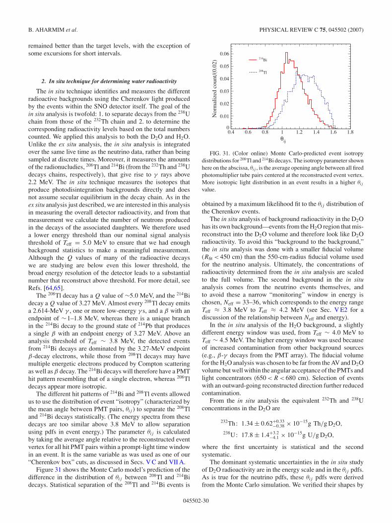
B. AHARMIM et al. PHYSICAL REVIEW C 75, 045502 (2007)
remained better than the target levels, with the exception ofsome excursions for short intervals.
2. In situ technique for determining water radioactivity
The in situ technique identifies and measures the differentradioactive backgrounds using the Cherenkov light producedby the events within the SNO detector itself. The goal of thein situ analysis is twofold: 1. to separate decays from the 238Uchain from those of the 232Th chain and 2. to determine thecorresponding radioactivity levels based on the total numberscounted. We applied this analysis to both the D2O and H2O.Unlike the ex situ analysis, the in situ analysis is integratedover the same live time as the neutrino data, rather than beingsampled at discrete times. Moreover, it measures the amountsof the radionucludies, 208Tl and 214Bi (from the 232Th and 238Udecays chains, respectively), that give rise to γ rays above2.2 MeV. The in situ technique measures the isotopes thatproduce photodisintegration backgrounds directly and doesnot assume secular equilibrium in the decay chain. As in theex situ analysis just described, we are interested in this analysisin measuring the overall detector radioactivity, and from thatmeasurement we calculate the number of neutrons producedin the decays of the associated daughters. We therefore useda lower energy threshold than our nominal signal analysisthreshold of Teff = 5.0 MeV to ensure that we had enoughbackground statistics to make a meaningful measurement.Although the Q values of many of the radioactive decayswe are studying are below even this lower threshold, thebroad energy resolution of the detector leads to a substantialnumber that reconstruct above threshold. For more detail, seeRefs. [64,65].
The 208Tl decay has a Q value of ∼5.0 MeV, and the 214Bidecay a Q value of 3.27 MeV. Almost every 208Tl decay emitsa 2.614-MeV γ , one or more low-energy γ s, and a β with anendpoint of ∼1–1.8 MeV, whereas there is a unique branchin the 214Bi decay to the ground state of 214Pb that producesa single β with an endpoint energy of 3.27 MeV. Above ananalysis threshold of Teff ∼ 3.8 MeV, the detected eventsfrom 214Bi decays are dominated by the 3.27-MeV endpointβ-decay electrons, while those from 208Tl decays may havemultiple energetic electrons produced by Compton scatteringas well as β decay. The 214Bi decays will therefore have a PMThit pattern resembling that of a single electron, whereas 208Tldecays appear more isotropic.
The different hit patterns of 214Bi and 208Tl events allowedus to use the distribution of event “isotropy” (characterized bythe mean angle between PMT pairs, θij ) to separate the 208Tland 214Bi decays statistically. (The energy spectra from thesedecays are too similar above 3.8 MeV to allow separationusing pdfs in event energy.) The parameter θij is calculatedby taking the average angle relative to the reconstructed eventvertex for all hit PMT pairs within a prompt-light time windowin an event. It is the same variable as was used as one of our“Cherenkov box” cuts, as discussed in Secs. V C and VII A.
Figure 31 shows the Monte Carlo model’s prediction of thedifference in the distribution of θij between 208Tl and 214Bidecays. Statistical separation of the 208Tl and 214Bi events is
θij
Nor
mal
ized
cou
nt/(
0.02
) 214Bi
208Tl
0
0.01
0.02
0.03
0.04
0.05
0.06
0.4 0.6 0.8 1 1.2 1.4 1.6 1.8
FIG. 31. (Color online) Monte Carlo-predicted event isotropydistributions for 208Tl and 214Bi decays. The isotropy parameter shownhere on the abscissa, θij , is the average opening angle between all firedphotomultiplier tube pairs centered at the reconstructed event vertex.More isotropic light distribution in an event results in a higher θij
value.
obtained by a maximum likelihood fit to the θij distribution ofthe Cherenkov events.
The in situ analysis of background radioactivity in the D2Ohas its own background—events from the H2O region that mis-reconstruct into the D2O volume and therefore look like D2Oradioactivity. To avoid this “background to the background,”the in situ analysis was done with a smaller fiducial volume(Rfit < 450 cm) than the 550-cm-radius fiducial volume usedfor the neutrino analysis. Ultimately, the concentrations ofradioactivity determined from the in situ analysis are scaledto the full volume. The second background in the in situanalysis comes from the neutrino events themselves, andto avoid these a narrow “monitoring” window in energy ischosen, Neff = 33–36, which corresponds to the energy rangeTeff ≈ 3.8 MeV to Teff ≈ 4.2 MeV (see Sec. V E2 for adiscussion of the relationship between Neff and energy).
In the in situ analysis of the H2O background, a slightlydifferent energy window was used, from Teff ∼ 4.0 MeV toTeff ∼ 4.5 MeV. The higher energy window was used becauseof increased contamination from other background sources(e.g., β-γ decays from the PMT array). The fiducial volumefor the H2O analysis was chosen to be far from the AV and D2Ovolume but well within the angular acceptance of the PMTs andlight concentrators (650 < R < 680 cm). Selection of eventswith an outward-going reconstructed direction further reducedcontamination.
From the in situ analysis the equivalent 232Th and 238Uconcentrations in the D2O are
232Th: 1.34 ± 0.62+0.33−0.38 × 10⁻¹⁵g Th/g D2O,
238U: 17.8 ± 1.4+3.2−4.1 × 10⁻¹⁵g U/g D2O,
where the first uncertainty is statistical and the secondsystematic.
The dominant systematic uncertainties in the in situ studyof D2O radioactivity are in the energy scale and in the θij pdfs.As is true for the neutrino pdfs, these θij pdfs were derivedfrom the Monte Carlo simulation. We verified their shapes by
045502-30
DETERMINATION OF THE νe AND . . . . I DATA SET PHYSICAL REVIEW C 75, 045502 (2007)
comparing them to the distributions obtained during periodsof Rn ingress into the target volume.
Temporal variation of the detector energy scale wasmodeled to study its effect on the extracted 232Th and 238U con-centrations. We have included in the systematic uncertaintiesresulting from contamination from other background sourcesin the monitoring window. In addition, we have includeduncertainties from potential nonuniformities of the spatialdistributions, and thus the numbers represent the estimateof the total radioactivity in the D2O, not just that withinR < 450 cm.
Similarly, the equivalent 232Th and 238U concentrations inthe H2O determined from the in situ analysis are
232 Th: 14.2 ± 0.6 ± 6.6 × 10⁻¹⁴g Th/g H2O,
238 U: 75.5 ± 1.2 ± 32.9 × 10⁻¹⁴g U/g H2O,
where again the statistical uncertainty is listed first.The systematic uncertainties in the H2O analysis are
considerably larger than those in the D2O analysis, with thelargest component in the H2O analysis being the contributionfrom the energy scale uncertainty, whose magnitude is 42%of the measured 232Th and 238U concentrations. The largeuncertainty is due, in part, to the fact that the optics of theouter regions of the detector are difficult to model (particularlythe optics of the PMT and concentrator assembly) and that wecalibrated these outer regions less frequently than the innerfiducial region.
3. Overall 232Th and 238U concentration determined for the water
The in situ and ex situ techniques are independent, and theirsystematic uncertainties have been independently assessed.Figure 30 shows good agreement between ex situ (232Th:MnOx, 238U: Rn assay) and in situ measurements. For the232Th chain, we have therefore used the weighted mean ofthe results, including additional uncertainties associated withthe ex situ sampling. The 238U chain activity is dominatedby Rn ingress, which is highly time dependent, and we havetherefore used the in situ determination for this activity as itincludes the appropriate weighting of neutrino live time. Forthe present data set, we find the equivalent equilibrium 238Uand 232Th concentrations in the D2O to be
232Th: 1.61 ± 0.58 × 10⁻¹⁵g Th/g D2O,
238U: 17.8+3.5−4.3 × 10⁻¹⁵g U/g D2O,
where we have added the statistical and systematic uncertain-ties in quadrature. The concentrations in the H2O are
232Th: 9.1 ± 2.7 × 10⁻¹⁴g Th/g H2O,
238U: 75.5 ± 33.0 × 10⁻¹⁴g U/g H2O.
4. Acrylic vessel radioactivity
To determine the photodisintegration background fromradioactivity in the walls of the AV, we first need to establish
the vessel’s radioactivity load. It is difficult to apply thein situ technique, primarily because the vessel is very cleanand its Cherenkov signals are masked by the dominant H2Obackground. The approach here is therefore to first determinethe radioactivity load of the AV from radioassay results,and then to use Monte Carlo simulations to deduce thephotodisintegration background. In the following, we discusscontributions to the radioactivity from the AV panels andbonds, from surface activity caused by mine dust, and from a“hot spot” of unknown origin.
During the production of the AV panels, acrylic sampleswere analyzed for internal 232Th and 238U radioactivities byneutron activation analysis. The 232Th concentration in thethermoformed acrylic panels was found to be 0.25 ± 0.04 ppt232Th.
Additional radioactivity was presumably introduced duringbonding of the acrylic panels, possibly from the glue, environ-mental dust, or plating of radioactive isotopes. It is difficultto determine this background, as dust might be embedded inthe bond during the construction. The surface area and volumeof the bonds are much smaller than those of the vessel asa whole, and therefore we estimate an uncertainty of +1
−0 µg232Th (∼total amount of Th from dust on the inner surfaceof the vessel) from embedded dust in the bonds. Adding thisin quadrature to the uncertainty of the Th concentration inthe thermoformed panels, we estimate 7.5+1.7
−1.3 µg of 232Th forthe full vessel. This represents an expected 6.2+1.4
−1.1 detectedphotodisintegration neutrons in the full Phase I data set.
Since the U contribution to the backgrounds is less than232Th for a given concentration and the U-to-Th ratio inmaterials is normally less than 1, the 238U concentration in thevessel did not pose as significant a problem as 232Th. Neutronactivation of virgin acrylic samples gave 2σ upper limitsranging from 0.1 to 1 ppt 238U. We therefore estimate 0.5±0.5ppt 238U as the total contamination, under the assumptionsthat the thermoforming process introduced the same amountof 238U into the panels as Th (∼0.2 ppt) and that the embeddeddust in the bonds has the same U-to-Th ratio as mine dust. Thistranslates to 15±15 µg 238U in the vessel.
During its construction and after final cleaning, the arealdensity of 232Th deposited on the surface of the AV wasdetermined from x-ray fluorescence (XRF) analysis of dustsamples lifted off the vessel’s surface by adhesive tapes. Theamount of 232Th on the AV determined from the XRF analysisafter its final cleaning was found to be
inner AV surface: 0.87 ± 0.17 µg 232Th,
outer AV surface: 0.96 ± 0.19 µg 232Th.
The 238U load could not be determined directly from the dustsample because of the limited sensitivity of the XRF. The dustsample was assumed to have the same composition as minedust—a 238U/232Th ratio of 0.187±0.024. The amount of 238Uon the AV is then
inner AV surface: 0.16 ± 0.04 µg 238U,
outer AV surface: 0.18 ± 0.04 µg 238U.
045502-31
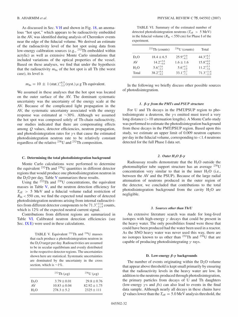
B. AHARMIM et al. PHYSICAL REVIEW C 75, 045502 (2007)
As discussed in Sec. V H and shown in Fig. 18, an anoma-lous “hot spot,” which appears to be radioactivity embeddedin the AV, was identified during analysis of Cherenkov eventsnear the edge of the fiducial volume. We derived an estimateof the radioactivity level of the hot spot using data fromlow-energy calibration sources (e.g., 232Th embedded withinacrylic) as well as extensive Monte Carlo simulations thatincluded variations of the optical properties of the vessel.Based on these analyses, we find that under the hypothesisthat the radioactivity mhs of the hot spot is all Th (the worstcase), its level is
mhs = 10 ± 1 (stat.)+8.5−3.5 (syst.) µ g Th equivalent.
We assumed in these analyses that the hot spot was locatedon the outer surface of the AV. The dominant systematicuncertainty was the uncertainty of the energy scale at theAV. Because of the complicated light propagation in theAV, the systematic uncertainty associated with the energyresponse was estimated at ∼30%. Although we assumedthe hot spot was composed solely of Th-chain radioactivity,our studies indicated that there are compensating effectsamong Q values, detector efficiencies, neutron propagation,and photodisintegration rates for γ s that cause the estimatedphotodisintegration neutron rate to be relatively constantregardless of the relative 238U and 232Th composition.
C. Determining the total photodisintegration background
Monte Carlo calculations were performed to determinethe equivalent 232Th and 238U quantities in different detectorregions that would produce one photodisintegration neutron inthe D2O per day. Table V summarizes these results.
Using the 232Th and 238U concentrations, the equivalentmasses in Table V, and the neutron detection efficiency forTeff > 5 MeV and a fiducial volume radial restriction ofRfit < 550 cm, we find the expected total number of detectedphotodisintegration neutrons arising from internal radioactivi-ties from different detector components to be 71.3+11.6
−11.9 counts,which is 12% of the expected neutral current signal.
Contributions from different regions are summarized inTable VI. Calibrated neutron detection efficiencies (seeSec. IX E) were used in these calculations.
TABLE V. Equivalent 232Th and 238U massesthat each produce a photodisintegration neutron inthe D2O target per day. Radioactivities are assumedto be in secular equilibrium and evenly distributedin the respective detector regions. The uncertaintiesshown here are statistical. Systematic uncertaintiesare dominated by the uncertainty in the crosssection, which is ∼1%.
232Th (µg) 238U (µg)
D2O 3.79 ± 0.01 29.8 ± 0.76AV 10.83 ± 0.04 82.92 ± 1.75H2O 278.3 ± 5.2 2325 ± 111
TABLE VI. Summary of the estimated number ofdetected photodisintegration neutrons (Teff > 5 MeV)in the fiducial volume (Rfit < 550 cm) for Phase I of theexperiment.
232Th (counts) 238U (counts) Total
D2O 18.4 ± 6.5 25.9+5.0−6.3 44.3+8.2
−9.1
AV 14.2+5.8−6.6 1.6 ± 1.6 15.8+6.0
−6.8
H2O 5.6+3.6−2.2 5.6+4.2
−2.9 11.2+5.5−3.6
Total 38.2+9.4−9.5 33.1+6.7
−7.1 71.3+11.6−11.9
In the following we briefly discuss other possible sourcesof photodisintegration.
1. β-γ from the PMTs and PSUP structure
For U and Th decays in the PMT/PSUP region to pho-todisintegrate a deuteron, the γ s emitted must travel a verylong distance (>10 attenuation lengths). A Monte Carlo studywas performed to estimate the photodisintegration backgroundfrom these decays in the PMT/PSUP region. Based upon thisstudy, we estimate an upper limit of 0.009 neutron capturesper day in the fiducial volume, corresponding to <1.4 neutronsdetected for the full Phase I data set.
2. Outer H2O β-γ
Radioassay results demonstrate that the H2O outside thephotomultiplier tube support structure has an average 238Uconcentration very similar to that in the inner H2O (i.e.,between the AV and the PSUP). Because of the large radialattenuation of neutrons produced in the outer region ofthe detector, we concluded that contributions to the totalphotodisintegration background from the cavity H2O arenegligible.
3. Sources other than Th/U
An extensive literature search was made for long-livedisotopes with high-energy γ decays that could be present inthe heavy water. The only possibilities found were those thatcould have been produced had the water been used in a reactor.As the SNO heavy water was never used this way, there areno isotopes known to us other than 232Th and 238U that arecapable of producing photodisintegrating γ rays.
D. Low-energy β-γ backgrounds
The number of events originating within the D2O volumethat appear above threshold is kept small primarily by ensuringthat the radioactivity levels in the heavy water are low. Inaddition to the neutrons produced through photodisintegration,the primary particles from decays of U and Th daughters(low-energy γ s and βs) can also lead to events in the finaldata sample. Although nearly all decays in these chains haveQ values lower than the Teff = 5.0 MeV analysis threshold, the
045502-32
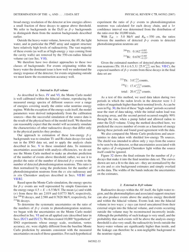
DETERMINATION OF THE νe AND . . . . I DATA SET PHYSICAL REVIEW C 75, 045502 (2007)
broad energy resolution of the detector at low energies allowsa small fraction of these decays to appear above threshold.We refer to backgrounds in the D2O as β-γ backgroundsto distinguish them from the neutron backgrounds describedearlier.
Outside the heavy-water volume, however, the AV, the lightwater, and in particular the PMT array and support structurehave relatively high levels of radioactivity. The vast majorityof these events (as well as of high-energy γ rays coming fromthe cavity walls) are removed by the 550-cm-radius fiducialvolume cut (see Sec. V H).
We therefore have two distinct approaches to these twoclasses of backgrounds: For events originating within theheavy water the dominant issue is how well we understand theenergy response of the detector; for events originating outsidewe must know the reconstruction accuracy well.
1. Internal to D2O volume
As described in Secs. IV and VI, the Monte Carlo modelis well calibrated within the fiducial volume, reproducing themeasured energy spectra of different sources over a rangeof energies covering nearly the entire solar neutrino energyregime. With the exception of the energy scale itself, the modelparameters were derived independently from the calibrationsources—thus the successful simulation of the source data isthe result of the physical basis of the model itself. We thereforecan reasonably expect that the model will accurately simulatethe characteristics of other radioactive decays that differ onlyin the physical particles they produce.
Our approach to estimation of these low-energy β-γbackgrounds was to simulate Tl- and Bi-chain decays for eachrun in the SNO data set, and to apply the analysis chaindescribed in Sec. V to these simulated data. To minimizeuncertainties associated with analysis efficiencies, we do notuse the Monte Carlo method to make an absolute predictionof the number of events above threshold; rather, we use it topredict the ratio of the number of detected β-γ events to thenumber of detected photodisintegration neutrons. This ratio isthen normalized by using the predictions for the number ofphotodisintegration neutrons from the ex situ radioassay andin situ Cherenkov analyses described in Secs. VII B1 andVII B2.
Based upon the Monte Carlo simulation, the energy spectrafor β-γ events are well represented by simple Gaussians inthe energy range 4.5 < E < 6.5 MeV. The mean (µ) and width(σ ) from these fits are 2.019 and 0.8773 MeV, respectively,for 208Tl decays, and 2.588 and 0.7828 MeV, respectively, for214Bi decays.
To determine the systematic uncertainties on the ratio ofthe numbers of β-γ events to photodisintegration neutrons,we began with the uncertainties on the Monte Carlo modeldescribed in Sec. VI and on all applied cuts (described later inSecs. IX C1 and IX C3). We then created 10,000 “hypothetical”SNO experiments whose energy scale, resolution, vertexaccuracy, etc. were slightly different from the baseline MonteCarlo prediction by amounts consistent with the measureduncertainties on each of those quantities. For each hypothetical
experiment the ratio of β-γ events to photodisintegrationneutrons was calculated for each decay chain, and a 1σ
confidence interval was determined from the distribution ofthe ratio over the 10,000 trials.
With Teff > 5.0 MeV and Rfit < 550 cm, the ratiosbetween the numbers of detected β-γ events to detectedphotodisintegration neutrons are
208Tl : 0.162+0.092−0.030,
214Bi: 0.670+0.460−0.125.
Given the estimated numbers of detected photodisintegra-tion neutrons (Th: 18.4 ± 6.5, U: 25.9+5.0
−6.3; see Sec. VII C), theexpected numbers of β-γ events from these decays in the finaldata set are
232Th: 3.0+2.0−1.3 counts,
238U: 17.4+12.4−5.3 counts,
total : 20.4+12.6−5.5 counts.
As a test of this method, we used data taken during twoperiods in which the radon levels in the detector were 1–2orders of magnitude higher than their nominal levels. As can beseen in Fig. 30, the first of these “high-radon” periods occurrednear the start of data taking, while the initial radon load wasdecaying away, and the second period occurred roughly 90%through the run, when a pump failed and allowed radon toenter the D2O volume. Using the method described here, wepredicted the excess number of events as a function of energyduring these periods and found good agreement with the data.
We also compared the Monte Carlo predictions and uncer-tainties to data taken with shielded low-energy Th sources.The shield was intended to allow only γ rays from the sourceto be seen by the detector, so that uncertainties associated withthe optics of β-originated Cherenkov light within the sourceitself could be ignored.
Figure 32 shows the final estimate for the number of β-γdecays that make it into the final neutrino data set. The curvesshown are not a fit to the data set—they are normalized by thein situ and ex situ background estimates and simply overlaidon the data. The widths of the bands indicate the uncertaintieson the estimates.
2. External to D2O volume
Radioactive decays within the AV itself, the light-water re-gion, and the photomultipliers and associated support structurecan also produce events above the analysis energy thresholdand within the fiducial volume. Events leak into the fiducialvolume in two ways: γ rays can travel unscattered from theirexternal origin into the fiducial volume, and events occurringoutside the volume may be reconstructed incorrectly inside.Although the probability of such leakage is very small, and theprobability that such events will be above the analysis energythreshold is also very small, the radioactivity levels outside theheavy-water volume are significantly higher than inside, andthe leakage can therefore be a non-negligible background tothe neutrino signal.
045502-33
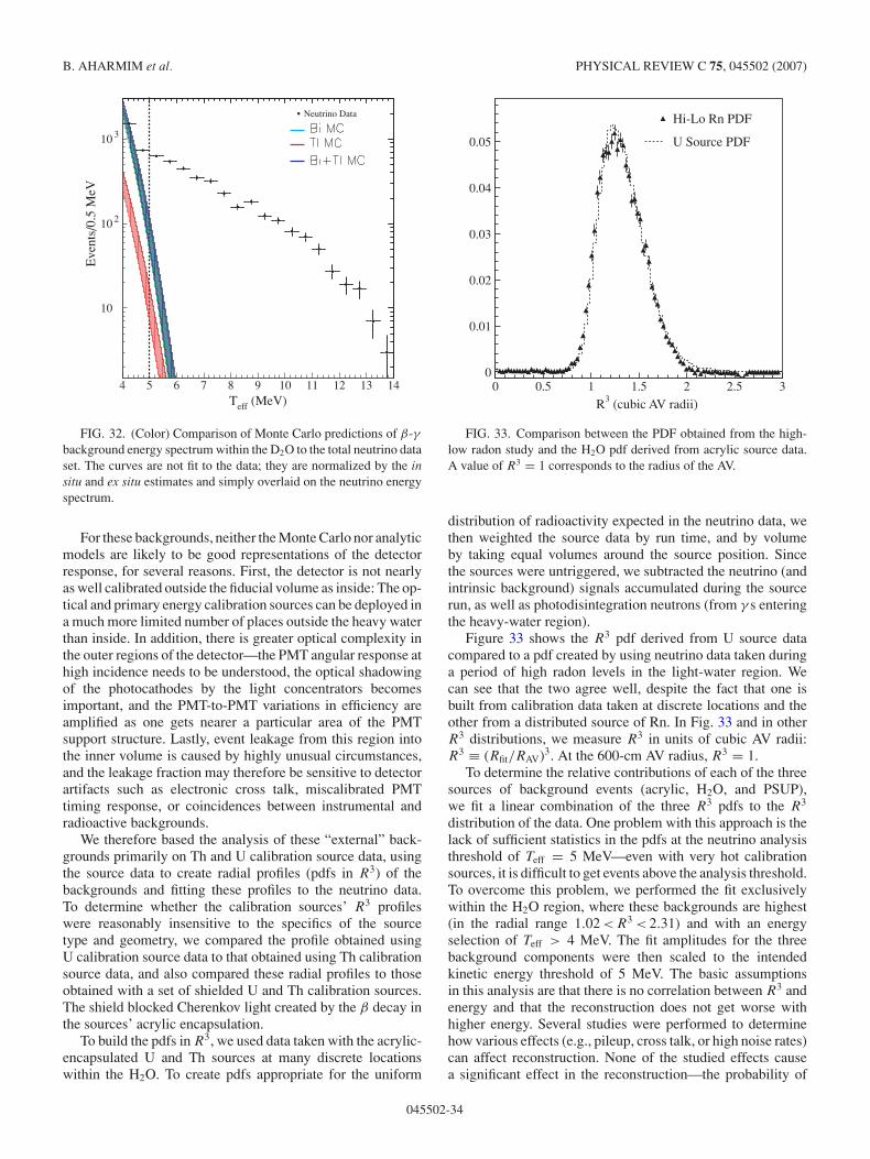
B. AHARMIM et al. PHYSICAL REVIEW C 75, 045502 (2007)
Neutrino Data
Teff (MeV)
Eve
nts/
0.5
MeV
10
10 2
10 3
4 5 6 7 8 9 10 11 12 13 14
FIG. 32. (Color) Comparison of Monte Carlo predictions of β-γbackground energy spectrum within the D2O to the total neutrino dataset. The curves are not fit to the data; they are normalized by the insitu and ex situ estimates and simply overlaid on the neutrino energyspectrum.
For these backgrounds, neither the Monte Carlo nor analyticmodels are likely to be good representations of the detectorresponse, for several reasons. First, the detector is not nearlyas well calibrated outside the fiducial volume as inside: The op-tical and primary energy calibration sources can be deployed ina much more limited number of places outside the heavy waterthan inside. In addition, there is greater optical complexity inthe outer regions of the detector—the PMT angular response athigh incidence needs to be understood, the optical shadowingof the photocathodes by the light concentrators becomesimportant, and the PMT-to-PMT variations in efficiency areamplified as one gets nearer a particular area of the PMTsupport structure. Lastly, event leakage from this region intothe inner volume is caused by highly unusual circumstances,and the leakage fraction may therefore be sensitive to detectorartifacts such as electronic cross talk, miscalibrated PMTtiming response, or coincidences between instrumental andradioactive backgrounds.
We therefore based the analysis of these “external” back-grounds primarily on Th and U calibration source data, usingthe source data to create radial profiles (pdfs in R3) of thebackgrounds and fitting these profiles to the neutrino data.To determine whether the calibration sources’ R3 profileswere reasonably insensitive to the specifics of the sourcetype and geometry, we compared the profile obtained usingU calibration source data to that obtained using Th calibrationsource data, and also compared these radial profiles to thoseobtained with a set of shielded U and Th calibration sources.The shield blocked Cherenkov light created by the β decay inthe sources’ acrylic encapsulation.
To build the pdfs in R3, we used data taken with the acrylic-encapsulated U and Th sources at many discrete locationswithin the H2O. To create pdfs appropriate for the uniform
R3 (cubic AV radii)
Hi-Lo Rn PDF
U Source PDF
0
0.01
0.02
0.03
0.04
0.05
0 0.5 1 1.5 2 2.5 3
FIG. 33. Comparison between the PDF obtained from the high-low radon study and the H2O pdf derived from acrylic source data.A value of R3 = 1 corresponds to the radius of the AV.
distribution of radioactivity expected in the neutrino data, wethen weighted the source data by run time, and by volumeby taking equal volumes around the source position. Sincethe sources were untriggered, we subtracted the neutrino (andintrinsic background) signals accumulated during the sourcerun, as well as photodisintegration neutrons (from γ s enteringthe heavy-water region).
Figure 33 shows the R3 pdf derived from U source datacompared to a pdf created by using neutrino data taken duringa period of high radon levels in the light-water region. Wecan see that the two agree well, despite the fact that one isbuilt from calibration data taken at discrete locations and theother from a distributed source of Rn. In Fig. 33 and in otherR3 distributions, we measure R3 in units of cubic AV radii:R3 ≡ (Rfit/RAV)3. At the 600-cm AV radius, R3 = 1.
To determine the relative contributions of each of the threesources of background events (acrylic, H2O, and PSUP),we fit a linear combination of the three R3 pdfs to the R3
distribution of the data. One problem with this approach is thelack of sufficient statistics in the pdfs at the neutrino analysisthreshold of Teff = 5 MeV—even with very hot calibrationsources, it is difficult to get events above the analysis threshold.To overcome this problem, we performed the fit exclusivelywithin the H2O region, where these backgrounds are highest(in the radial range 1.02 < R3 < 2.31) and with an energyselection of Teff > 4 MeV. The fit amplitudes for the threebackground components were then scaled to the intendedkinetic energy threshold of 5 MeV. The basic assumptionsin this analysis are that there is no correlation between R3 andenergy and that the reconstruction does not get worse withhigher energy. Several studies were performed to determinehow various effects (e.g., pileup, cross talk, or high noise rates)can affect reconstruction. None of the studied effects causea significant effect in the reconstruction—the probability of
045502-34
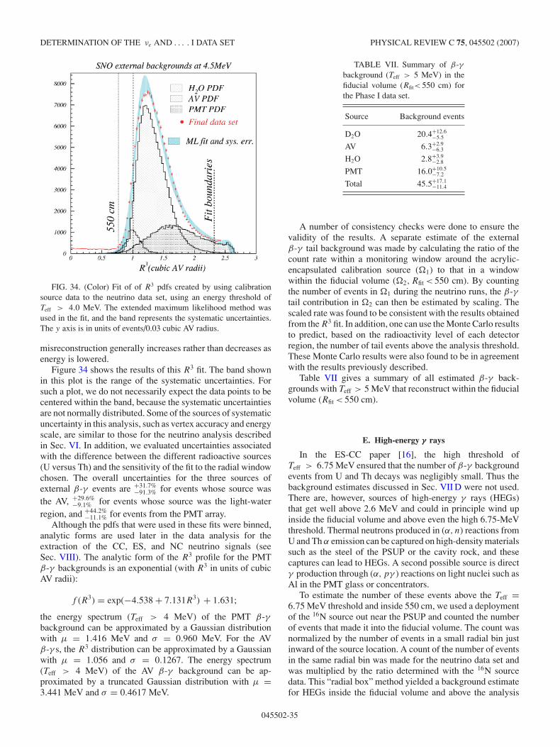
DETERMINATION OF THE νe AND . . . . I DATA SET PHYSICAL REVIEW C 75, 045502 (2007)
FIG. 34. (Color) Fit of of R3 pdfs created by using calibrationsource data to the neutrino data set, using an energy threshold ofTeff > 4.0 MeV. The extended maximum likelihood method wasused in the fit, and the band represents the systematic uncertainties.The y axis is in units of events/0.03 cubic AV radius.
misreconstruction generally increases rather than decreases asenergy is lowered.
Figure 34 shows the results of this R3 fit. The band shownin this plot is the range of the systematic uncertainties. Forsuch a plot, we do not necessarily expect the data points to becentered within the band, because the systematic uncertaintiesare not normally distributed. Some of the sources of systematicuncertainty in this analysis, such as vertex accuracy and energyscale, are similar to those for the neutrino analysis describedin Sec. VI. In addition, we evaluated uncertainties associatedwith the difference between the different radioactive sources(U versus Th) and the sensitivity of the fit to the radial windowchosen. The overall uncertainties for the three sources ofexternal β-γ events are +31.7%
−91.3% for events whose source wasthe AV, +29.6%
−9.1% for events whose source was the light-waterregion, and +44.2%
−11.1% for events from the PMT array.Although the pdfs that were used in these fits were binned,
analytic forms are used later in the data analysis for theextraction of the CC, ES, and NC neutrino signals (seeSec. VIII). The analytic form of the R3 profile for the PMTβ-γ backgrounds is an exponential (with R3 in units of cubicAV radii):
f (R3) = exp(−4.538 + 7.131R3) + 1.631;
the energy spectrum (Teff > 4 MeV) of the PMT β-γbackground can be approximated by a Gaussian distributionwith µ = 1.416 MeV and σ = 0.960 MeV. For the AVβ-γ s, the R3 distribution can be approximated by a Gaussianwith µ = 1.056 and σ = 0.1267. The energy spectrum(Teff > 4 MeV) of the AV β-γ background can be ap-proximated by a truncated Gaussian distribution with µ =3.441 MeV and σ = 0.4617 MeV.
TABLE VII. Summary of β-γbackground (Teff > 5 MeV) in thefiducial volume (Rfit< 550 cm) forthe Phase I data set.
Source Background events
D2O 20.4+12.6−5.5
AV 6.3+2.9−6.3
H2O 2.8+3.9−2.8
PMT 16.0+10.5−7.2
Total 45.5+17.1−11.4
A number of consistency checks were done to ensure thevalidity of the results. A separate estimate of the externalβ-γ tail background was made by calculating the ratio of thecount rate within a monitoring window around the acrylic-encapsulated calibration source (�1) to that in a windowwithin the fiducial volume (�2, Rfit < 550 cm). By countingthe number of events in �1 during the neutrino runs, the β-γtail contribution in �2 can then be estimated by scaling. Thescaled rate was found to be consistent with the results obtainedfrom the R3 fit. In addition, one can use the Monte Carlo resultsto predict, based on the radioactivity level of each detectorregion, the number of tail events above the analysis threshold.These Monte Carlo results were also found to be in agreementwith the results previously described.
Table VII gives a summary of all estimated β-γ back-grounds with Teff > 5 MeV that reconstruct within the fiducialvolume (Rfit < 550 cm).
E. High-energy γ rays
In the ES-CC paper [16], the high threshold ofTeff > 6.75 MeV ensured that the number of β-γ backgroundevents from U and Th decays was negligibly small. Thus thebackground estimates discussed in Sec. VII D were not used.There are, however, sources of high-energy γ rays (HEGs)that get well above 2.6 MeV and could in principle wind upinside the fiducial volume and above even the high 6.75-MeVthreshold. Thermal neutrons produced in (α, n) reactions fromU and Th α emission can be captured on high-density materialssuch as the steel of the PSUP or the cavity rock, and thesecaptures can lead to HEGs. A second possible source is directγ production through (α, pγ ) reactions on light nuclei such asAl in the PMT glass or concentrators.
To estimate the number of these events above the Teff =6.75 MeV threshold and inside 550 cm, we used a deploymentof the 16N source out near the PSUP and counted the numberof events that made it into the fiducial volume. The count wasnormalized by the number of events in a small radial bin justinward of the source location. A count of the number of eventsin the same radial bin was made for the neutrino data set andwas multiplied by the ratio determined with the 16N sourcedata. This “radial box” method yielded a background estimatefor HEGs inside the fiducial volume and above the analysis
045502-35
B. AHARMIM et al. PHYSICAL REVIEW C 75, 045502 (2007)
energy threshold of <0.8%. For more details of this method,see Ref. [28].
For the NC [17] results, we found that the fit in R3
for the external β-γ background described in Sec. VII D2already accounted for the HEG background through the pdffor the PMT β-γ s. We thus did not include an independentestimate of these events for the NC paper, and the third line ofTable VII should be taken to include the contribution fromthese high-energy γ rays.
F. Additional sources of neutrons
In addition to the photodisintegration backgrounds dis-cussed in Sec. VII B, there are other possible sources ofneutrons:
(i) spontaneous fission of 238U or 252Cf;(ii) neutrons from cosmogenic sources;
(iii) deuteron breakup from α reactions;(iv) neutron production from (α,n) reactions; and(v) neutrons produced by terrestrial and reactor antineutri-
nos.
These will be discussed in the following sections.
1. Spontaneous fission
Neutron backgrounds may arise from spontaneous fission of238U or 252Cf. Such fission events have unique characteristics,such as low-energy γ production and the presence of multipleneutrons. Many of these events are therefore removed throughthe burst cuts discussed in Sec. V and Appendix B, but herewe estimate an upper bound on the number remaining in thedata set.
The spontaneous fission half-life of 238U is 8.2 ± 0.1 ×10¹⁵ yr [66], corresponding to a branching ratio of 5.45×10⁻⁷.The contribution of the spontaneous fission of 238U to neutronbackgrounds can be based on the measured concentration of226Ra, but such an inference relies on the assumption thatthe uranium decay chain is in equilibrium above radon.Alternatively, we can use ex situ measurements of 238U fromthe HTiO adsorbent technique to determine the contributionfrom uranium directly. Measurements of 238U from HTiOradioassays indicate less than (10−15 g 238U)/g in the D2Ovolume. At such concentrations, the contribution of sponta-neous fission to the neutron background is much less than 1event.
Spontaneous fission of 252Cf, introduced through thedeployment of the encapsulated neutron calibration source,can also occur. Based upon our leach tests of the deployedsource, we estimate that it contributed much less than 1 eventto the final data set.
2. Cosmogenic sources
SNO’s great depth reduces the number of cosmic rayspassing through the detector to an extremely low rate—roughly three through-going muons per hour within the PSUP
enclosure. Nevertheless, cosmic rays—which include muonsas well as a low rate of atmospheric neutrino interactions withinthe detector volume—are a potential source of backgrounds.Cosmic-ray interactions may produce both radioactive nu-clides and neutrons. As described in Sec. V G, we used twocuts to remove these events. The first cut, intended to removeboth spallation nuclei and “follower neutrons,” eliminated allevents that occurred within 20 s of a tagged muon event. Thesecond, intended to remove neutrons produced by untaggedmuons and atmospheric neutrinos, removed all events in a250-ms window following any event with more than 60 hitPMTs.
After these cuts are made, there are still potential sources ofresidual background events; we address each of these in turn.
Followers of external muons. One potential source ofneutrons comes from muons passing outside the detectorvolume, through the light-water shield between the AV andthe PSUP, between the PSUP and the rock, or within the rock.These high-energy neutrons are typically produced throughphotonuclear interactions between the muon and nuclei inthe H2O and through secondary neutron production fromsubsequent interactions of the products of these reactions. Thehigh-energy neutrons can penetrate through the water shieldsurrounding the detector and contribute to the NC background.
To determine contamination from neutron events thatpassed through the light-water shield, we looked for followerevents inside the fiducial volume subsequent to events trig-gering the outward-looking (OWL) PMT array. We foundthat the number of these follower events was consistent withexpectations from accidental coincidences alone, and thereforethe external muons are not a significant source of backgroundin the final neutrino candidate sample.
We also estimated the number of neutrons produced frommuon interactions in the rock, using both analytical modelsand explicit Monte Carlo simulations. Our estimate places thetotal neutron event rate from muon-rock interactions below0.18 neutrons/yr, not including losses from reconstructionefficiencies.
Followers of internal muons. Neutrons created by muonspassing through the detector’s fiducial volume are removedthrough the muon follower cuts just described here and inSec. V G. The efficiency of the cut is extremely high, asonly a small fraction of (the already small number of)muons originating outside the detector and making it tothe fiducial volume will be below Cherenkov threshold andthus undetected. Extrapolating from the number of followerswe measure for detected muons, we find that the numberremaining in the data set after the muon follower cuts isnegligible, the one exception being the muons created inassociation with atmospheric neutrino interactions inside thedetector volume, which are discussed next.
Atmospheric neutrinos. The interactions of atmosphericneutrinos can produce primary events within the fiducial vol-ume of the detector, and the products of these events—eitherneutrons or spallation nuclei—can contaminate the final dataset. Only a small subset of atmospheric neutrino interactionscan mimic authentic solar neutrino events. Among these areneutral current events that release one or more neutrons,neutral current events where a photon is released from the
045502-36
DETERMINATION OF THE νe AND . . . . I DATA SET PHYSICAL REVIEW C 75, 045502 (2007)
de-excitation of 16O, or low-energy charged current reactions.These low-energy atmospheric neutrino interactions are oftenassociated with a burst of events in the detector and are thusremoved by the time-correlated cuts described in Sec. V C andAppendix B. To estimate the background from the events thatremain after the cuts, we made use of a combination of analyticcalculations of the rates of atmospheric neutrino interactionsand a full Monte Carlo simulation of the propagation of theirsecondaries within the SNO detector.
We estimated the flux of atmospheric neutrinos usingthe calculations of Agrawal et al. [67] for North Americanlatitudes during solar maximum, and we considered energyranges from 50 MeV to 10 GeV. We included neutrinooscillations, assuming the measured νµ → ντ parametersfrom the Super-Kamiokande Collaboration [68] (�m2 =3 × 10⁻³eV2 and sin2(2θ ) = 1), and took into account pathlengths through the Earth in the angular distribution of theflux. For these parameters, approximately 67% of the νµ eventsremain after oscillation.
To calculate the interaction rates, we used the formalism ofLlewellyn-Smith [69]. Since SNO possesses an isoscalar targetand the neutral current process does not distinguish neutrinoflavors, the ratio of neutral current neutron interactions withmuon charged current interactions is ≈0.54. By knowingthe relative efficiencies of the two types of events, we cannormalize to the observed partially contained muons in thedetector.
To estimate these efficiencies, the showers of particlesproduced in neutrino interactions were propagated through thedetector using SNO’s Monte Carlo simulation. We propagatethe muons and hadrons through the SNO Monte Carlosimulation using the FLUKA hadron propagation code [70].
The systematic uncertainties associated with the atmo-spheric neutrino event rate in SNO come mainly from un-certainties associated with the primary neutrino flux and fromthe nuclear final-state interactions. Other errors that arise in thecalculation include uncertainties in the axial mass associatedwith the quasi-elastic cross section [69], the application ofPauli suppression, uncertainties in the oscillation parameters,and uncertainties in the pion-resonance cross section. Thetotal uncertainty from the neutrino flux and cross-sectioncontributions is ±30%. Effects of final-state interactions aredealt with in the next section.
After applying our analysis cuts including fiducial volumeand energy threshold (as described in Sec. V) we find that thecombined background from all atmospheric neutrino sourcesis 4 ± 1 events for the Phase I data set.
Cosmogenic production of 16N and other radioactivity.When a high-energy muon enters the SNO detector, severalprocesses can produce long-lived radioactive nuclei. The mostcommon process is capture of a stopped muon on 16O, whichproduces a 16N nucleus. Another process is muon-inducedspallation, in which a muon splits a nucleus into smallerfragments, some or all of which may be radioactive. Theseradioactive nuclei can produce backgrounds to the neutralcurrent solar neutrino signal if they decay by the productionof a neutron, or if they produce a γ ray with an energyabove 2.2 MeV, which can photodisintegrate 2H. They can
also form a background to the charged current signal throughthe Cherenkov light generated via β or γ decays.
Cosmic-ray muons can also disintegrate 2H nuclei directly,producing prompt neutrons. The majority of these will captureand are removed by the muon follower cut. One mustalso consider muon capture on other nuclei, which mightproduce longer lived nuclei, and (n, p), (n, α), (p, n), and(p, α) reactions that produce long-lived nuclei.
The dominant contribution of cosmogenic radioactivity tothe background comes from the production of 16N, whichdecays with a half-life of 7.13 s, via either muon captureor (n, p) reactions. An experimental measurement of thisand other spallation products is obtainable from the timedependence of muon followers, which has been evaluated inseveral independent analyses. The presence of initial 16N isconsistent with accidental background activity and makes upa negligible portion of the total background rate.
3. Neutrons from (α, n) reactions
Decays in the uranium and thorium chains produce αs,which in turn can produce neutrons via the following reactions:
2H + α → n + 1H − 2.223 MeV,
13C + α → n + 16O + 2.251 MeV,
17O + α → n + 20Ne + 5.871 MeV,
18O + α → n + 21Ne − 0.689 MeV.
The molecular targets of interest in SNO that could lead tothese reactions are H2O, D2O, and acrylic—(C5H8O2)n. Theoxygen isotopes 17O and 18O are somewhat enriched in D2O;natural oxygen is composed of 0.038% 17O and 0.2% 18O,whereas the fractional isotopic abundances in the heavy waterare 0.0485(5)% and 0.320(3)%, respectively [71].
All 14 α decays in the uranium and thorium chains areabove threshold (6.6 MeV) for the (α, n) reactions listed here.The rates are 1.28 × 10⁵ and 3.92 × 10⁵ decays/yr/µg of232Th and 238U, respectively. In the heavy water, the mainsource of (α, n) is 222Rn. Contamination on the surface ofthe acrylic by radon daughters, however, could yield moreneutrons than expected from the U and Th present in the heavywater. Such neutrons would have a somewhat different radialprofile from neutrons generated in the D2O volume. As willbe discussed further in Sec. X C, in our Phase I publicationswe performed a fit to the data using the expected radial profileof external neutrons, allowing their number to float in the fit.We found in this fit that the total number of external neutronswas consistent with our estimates for photodisintegration byexternal radioactivity alone. In a future publication, we willinclude updates to the results here that explicitly fit for thispotential source of neutrons.
The neutron yields from 2H(α, αn)1H and from (α,n)reactions are summarized in Table VIII.
045502-37
B. AHARMIM et al. PHYSICAL REVIEW C 75, 045502 (2007)
TABLE VIII. Additional (non-photodisintegration)neutron and γ backgrounds in the SNO detector D2Ovolume (R < 550 cm). The last column gives the estimatedbackground contribution to the data set for Phase I, after allanalysis cuts have been applied. Portions of the neutron/γcontribution errors are anticorrelated.
Source Expected number ofdetected events
Fission [U,Cf] (neutrons) �1Fission [U,Cf] (γ s) �1Atmospheric ν 4 ± 12H(α, αn)1H [Th] 0.40 ± 0.132H(α, αn)1H [222Rn] 1.59 ± 0.3017,18O(α, n)20,21Ne [Th] �117,18O(α, n)20,21Ne [222Rn] �117,18O(α, n)20,21Ne [238U] �116N following muons �1Other spallation �1Muon follower neutrons �1Cosmogenic rock neutrons 0.18 ± 0.01Terrestrial and reactor ν 1+3
−1
Total additional neutrons and γ s 7+3−1
4. Neutron production from terrestrial and reactor antineutrinos
Antineutrino interactions with the light water, acrylic, andheavy water are an additional source of background neutrons.Such antineutrinos can be produced by radioactive decays ofuranium and thorium in the Earth’s crust and mantle, as wellas by nearby fission reactors [72].
Neutrons are produced in three antineutrino-induced reac-tions:
νe + p → n + e+ − 1.804 MeV (ccp), (31)
νe + d → n + n + e+ − 4.03 MeV (ccd), (32)
νx + d → p + n + νx − 2.223 MeV (ncd). (33)
The charged current reaction on protons (ccp) has athreshold of 1.804 MeV. There are four β decays in the uraniumand thorium decay chains that emit antineutrinos above thisthreshold. The charged current reaction on deuterium (ccd) hasa larger threshold of 4.03 MeV, so it need only be consideredfor reactor antineutrinos. The neutral current reaction (ncd)has a threshold of 2.223 MeV, and thus it must be consideredfor reactor antineutrinos and for antineutrinos from 214Bi in theuranium chain. There are two other decays, from 212Bi in thethorium chain and 234Pa in the uranium chain, with antineutrinoenergies of 2.25 and 2.29 MeV, respectively, that are above thencd reaction threshold. The amount by which they are overthreshold, however, is small and their contribution is assumedto be negligible.
In calculating the total contribution of antineutrinos to thebackground, effects such as vacuum oscillations, reactor livetimes, and reactor efficiencies have been taken into account.Table VIII shows the results. The tabulated numbers for thecharged current include the fact that each interaction producesnot one but two neutrons per interaction. These numbers are in
TABLE IX. Summary of estimated numbers of events foreach source of background.
Source Events
NeutronsD2O photodisintegration 44+8
−9
H2O+AV photodisintegration 27+8−8
Atmospheric νs andsub-Cherenkov threshold µs 4 ± 1
Fission �12H(α, α)pn 2 ± 0.417O(α, n) �1
Terrestrial and reactor νs 1+3−1
Cosmogenic neutrons from rock �1
Total neutron background 78 ± 12
β-γ s
D2O β-γ 20+13−6
H2O β-γ 3+4−3
AV β-γ 6+3−6
PMT β-γ (+HEGs) 16+11−8
Total β-γ background 45+18−12
InstrumentalTotal Instrumental <3
agreement with the background levels calculated for our limiton solar antineutrinos [73].
5. Summary of other neutron backgrounds
The neutron backgrounds from the sources discussed in thissection are summarized in Table VIII.
G. Overall background summary
Table IX summarizes all sources of background discussedin this section. As will be discussed in Secs. VIII andX, the background numbers are subtraced off of the final,fitted event totals. In the case of the β-γ backgrounds, thenumbers are used to fix the amplitudes of energy spectrumpdfs (the analytic forms of which were given in Secs. VII D1and VII D2) during the signal-extraction process. For theinternally produced neutron backgrounds, which look identicalto neutrons produced by neutrino NC reactions, the numbersare directly subtracted from the final fitted neutron event total.For external neutrons produced by radioactivity in the AV andH2O, a radial pdf is included in the signal-extraction fit withits amplitude fixed to the value given in the table.
VIII. SIGNAL-EXTRACTION METHOD
We have described the analysis used to build accuratemodels of neutrino and background signals in our detector,the processing of the data, and the measurement of thebackgrounds. After accomplishing those tasks we are in aposition to fit the data with the pdfs shown in Fig. 2. Thefit itself is an extended maximum likelihood method usingbinned pdfs. We used multiple sets of pdfs to verify ouroverall results. For example, we used both pdfs based on
045502-38
DETERMINATION OF THE νe AND . . . . I DATA SET PHYSICAL REVIEW C 75, 045502 (2007)
the reconstructed kinetic energies as shown in Fig. 2 anddescribed in Sec. V E and pdfs that used only the total numberof hits in each event (“Nhit”) as a measure of the event energy.These two approaches are identical, other than in the choice ofenergy variable. As a further check, we fit the data using pdfsconstructed from an analytic model rather than from MonteCarlo simulation.
There are alternate approaches to fitting the energy spectraof the data set. In one method, we constrain the recoil electronspectra of the CC and ES events to be that resulting froman undistorted 8B neutrino spectrum. This “constrained” fit isthus a test of the null hypothesis that solar neutrinos do notoscillate and is also appropriate for the case of an energy-independent νe survival probability, which is nearly correctfor the large mixng angle solution in this energy region. Analternate approach is to perform the fit without a constrainton the CC energy spectral shape. This may be done either byexcluding the energy variable from the signal extraction andso using a pdf only in R3 and cos θ�, as was done in our PhaseI NC paper [17], or by fitting the CC energy spectrum bin bybin while fixing the NC and background energy pdfs to theirknown shapes, as in the Phase I ES-CC paper [16].
We describe in this section the details of our signal-extraction method, and we leave the presentation of the fluxresults to Sec. X.
A. Extended maximum likelihood method
The basis of the signal extraction is to express the proba-bility distribution for neutrino events in the variables E,R3,and cos θ� with a linear superposition of pdfs corresponding todifferent signals and backgrounds. The total number of eventsν as a function of E,R3, and cos θ� is then
ν(E,R3, cos θ�) =∑
i
Nifi(E,R3, cos θ�), (34)
where Ni is the number of events of type i (e.g., CC, ES, orNC), and fi is the probability distribution for events of thattype, normalized to unity. The sum is taken over all signaltypes, and over classes of background events for which pdfsmay be constructed. In this section, we use E to mean eitherTeff or Nhit: the former for our primary signal extraction, whichuses the energy reconstructor, and the latter for the verificationsignal extraction, which uses the total light energy estimate.
The extended log likelihood then takes the form
logL = −∑
i
Ni +∑
j
nj ln[ν
(Ej ,R
3j , cos θ�j
)], (35)
where j is a sum over all three-dimensional bins in the threesignal-extraction parameters E,R3, and cos θ�, and nj is thenumber of detected events in each bin.
In this analysis the numbers of CC, ES, and NC eventsare treated as free parameters in the fit, while the numbersof background events of each type are fixed, as described inSec. VIII C. The likelihood function is maximized over thefree parameters, and the best-fit point yields the number ofCC, ES, and NC events along with a covariance matrix.
B. Fitting with Monte Carlo pdfs
Our reported results use the Monte Carlo simulation togenerate pdfs for the neutrino signals over the three signal-extraction variables: the effective kinetic energy Teff returnedby the energy calibrator (see Sec. V E), R3, and cos θ�.Generation of pdfs using the total number of hit PMTs(Nhit) was done similarly to what we describe here with thesubstitution of Nhit for Teff . (As mentioned in the previoussection, here the variable E will denote either Teff or Nhit.)
1. Monte Carlo pdf generation
The pdfs were constructed by binning simulated eventsin these three quantities, under the implicit assumption thatthe full three-dimensional pdf factorizes into separate energy,radial, and angular components:
F (E,R3, cos θ�) = A(E)B(R3)C(cos θ�). (36)
The functions A,B, and C in Eq. (36) are shown in Fig. 2.There are, in fact, modest correlations between energy and
R3 at the few percent level, as well as a narrowing of the widthof the elastic scattering angular peak with increasing energy.By testing the signal-extraction procedure on many sampleMonte Carlo data sets, we verified that these correlationsintroduced negligible bias in the extracted fluxes and couldtherefore be ignored.
The Monte Carlo simulations used to create the pdfs wereperformed run-by-run, matching the simulation inputs to thestate of the detector for each run as described in Sec. IV I. Thesimulation for each run took account of the number of channelsonline, threshold settings, the average PMT noise rate derivedfrom the 5-Hz pulsed trigger, and the measured live time ofthe run. The statistics for the Monte Carlo runs were 50 timesthe Standard Solar Model (SSM) prediction for each of thesignals.
As described in Sec. V E, the mean energy response of thedetector varied slowly over the course of the data set. Thisvariation was incorporated into the calculation of the energyfor each event as a factor that depended upon the time ofthe event relative to the start of the data set. Monte Carlosimulations were done at a fixed energy scale.
For the analysis described in the ES-CC paper [16], theenergy component of the pdfs was binned in 34 unequalbins between the lower and upper energy limits of theanalysis (Teff = 6.75–19.5 MeV). The first 33 bins were each0.2574-MeV wide, and the final bin was extended up toTeff = 19.5 MeV. For the analysis in the Phase I NC paper [17],the energy component of the pdfs was binned in 42 binsbetween the lower and upper energy limits of the analysis(Teff = 5.0−19.5 MeV kinetic energy). Each of these bins was0.25-MeV wide, except for the last bin, which was extendedto the upper energy limit. In both the ES-CC paper and the NCpaper, the radial distribution was binned in 30 equal bins in R3
inside the 550-cm-radius fiducial volume, and the angular pdfswere binned in 30 unequal bins of cos θ�. Fifteen equal binsspanned the region −1 � cos θ� < 0.5, and the remaining 15bins spanned the region 0.5 � cos θ� < + 1. This unequal
045502-39
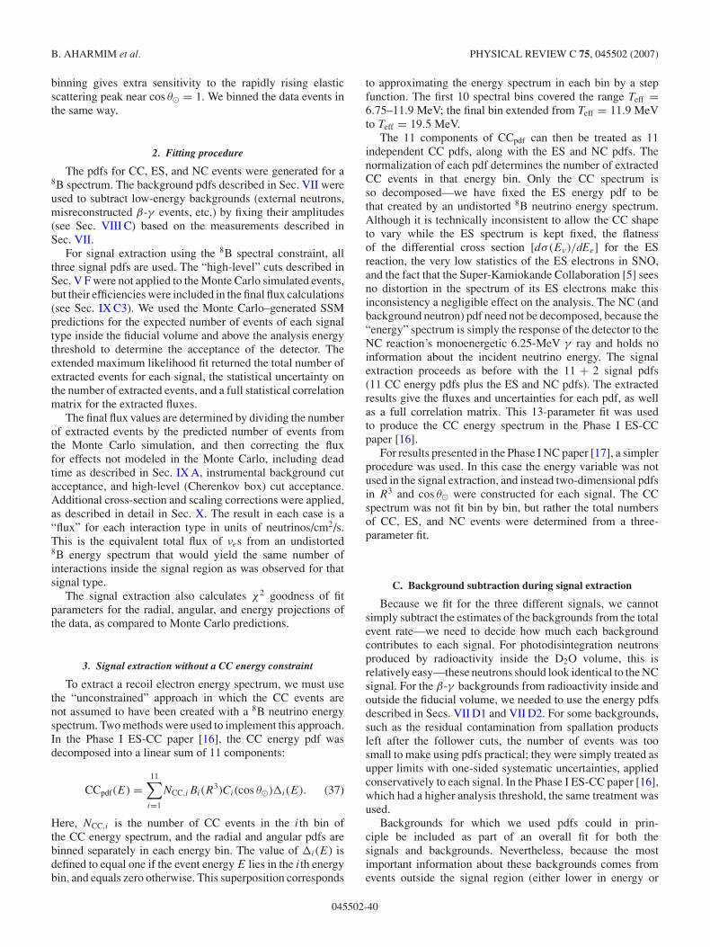
B. AHARMIM et al. PHYSICAL REVIEW C 75, 045502 (2007)
binning gives extra sensitivity to the rapidly rising elasticscattering peak near cos θ� = 1. We binned the data events inthe same way.
2. Fitting procedure
The pdfs for CC, ES, and NC events were generated for a8B spectrum. The background pdfs described in Sec. VII wereused to subtract low-energy backgrounds (external neutrons,misreconstructed β-γ events, etc.) by fixing their amplitudes(see Sec. VIII C) based on the measurements described inSec. VII.
For signal extraction using the 8B spectral constraint, allthree signal pdfs are used. The “high-level” cuts described inSec. V F were not applied to the Monte Carlo simulated events,but their efficiencies were included in the final flux calculations(see Sec. IX C3). We used the Monte Carlo–generated SSMpredictions for the expected number of events of each signaltype inside the fiducial volume and above the analysis energythreshold to determine the acceptance of the detector. Theextended maximum likelihood fit returned the total number ofextracted events for each signal, the statistical uncertainty onthe number of extracted events, and a full statistical correlationmatrix for the extracted fluxes.
The final flux values are determined by dividing the numberof extracted events by the predicted number of events fromthe Monte Carlo simulation, and then correcting the fluxfor effects not modeled in the Monte Carlo, including deadtime as described in Sec. IX A, instrumental background cutacceptance, and high-level (Cherenkov box) cut acceptance.Additional cross-section and scaling corrections were applied,as described in detail in Sec. X. The result in each case is a“flux” for each interaction type in units of neutrinos/cm2/s.This is the equivalent total flux of νes from an undistorted8B energy spectrum that would yield the same number ofinteractions inside the signal region as was observed for thatsignal type.
The signal extraction also calculates χ2 goodness of fitparameters for the radial, angular, and energy projections ofthe data, as compared to Monte Carlo predictions.
3. Signal extraction without a CC energy constraint
To extract a recoil electron energy spectrum, we must usethe “unconstrained” approach in which the CC events arenot assumed to have been created with a 8B neutrino energyspectrum. Two methods were used to implement this approach.In the Phase I ES-CC paper [16], the CC energy pdf wasdecomposed into a linear sum of 11 components:
CCpdf(E) =11∑i=1
NCC,iBi(R3)Ci(cos θ�)�i(E). (37)
Here, NCC,i is the number of CC events in the ith bin ofthe CC energy spectrum, and the radial and angular pdfs arebinned separately in each energy bin. The value of �i(E) isdefined to equal one if the event energy E lies in the ith energybin, and equals zero otherwise. This superposition corresponds
to approximating the energy spectrum in each bin by a stepfunction. The first 10 spectral bins covered the range Teff =6.75–11.9 MeV; the final bin extended from Teff = 11.9 MeVto Teff = 19.5 MeV.
The 11 components of CCpdf can then be treated as 11independent CC pdfs, along with the ES and NC pdfs. Thenormalization of each pdf determines the number of extractedCC events in that energy bin. Only the CC spectrum isso decomposed—we have fixed the ES energy pdf to bethat created by an undistorted 8B neutrino energy spectrum.Although it is technically inconsistent to allow the CC shapeto vary while the ES spectrum is kept fixed, the flatnessof the differential cross section [dσ (Eν)/dEe] for the ESreaction, the very low statistics of the ES electrons in SNO,and the fact that the Super-Kamiokande Collaboration [5] seesno distortion in the spectrum of its ES electrons make thisinconsistency a negligible effect on the analysis. The NC (andbackground neutron) pdf need not be decomposed, because the“energy” spectrum is simply the response of the detector to theNC reaction’s monoenergetic 6.25-MeV γ ray and holds noinformation about the incident neutrino energy. The signalextraction proceeds as before with the 11 + 2 signal pdfs(11 CC energy pdfs plus the ES and NC pdfs). The extractedresults give the fluxes and uncertainties for each pdf, as wellas a full correlation matrix. This 13-parameter fit was usedto produce the CC energy spectrum in the Phase I ES-CCpaper [16].
For results presented in the Phase I NC paper [17], a simplerprocedure was used. In this case the energy variable was notused in the signal extraction, and instead two-dimensional pdfsin R3 and cos θ� were constructed for each signal. The CCspectrum was not fit bin by bin, but rather the total numbersof CC, ES, and NC events were determined from a three-parameter fit.
C. Background subtraction during signal extraction
Because we fit for the three different signals, we cannotsimply subtract the estimates of the backgrounds from the totalevent rate—we need to decide how much each backgroundcontributes to each signal. For photodisintegration neutronsproduced by radioactivity inside the D2O volume, this isrelatively easy—these neutrons should look identical to the NCsignal. For the β-γ backgrounds from radioactivity inside andoutside the fiducial volume, we needed to use the energy pdfsdescribed in Secs. VII D1 and VII D2. For some backgrounds,such as the residual contamination from spallation productsleft after the follower cuts, the number of events was toosmall to make using pdfs practical; they were simply treated asupper limits with one-sided systematic uncertainties, appliedconservatively to each signal. In the Phase I ES-CC paper [16],which had a higher analysis threshold, the same treatment wasused.
Backgrounds for which we used pdfs could in prin-ciple be included as part of an overall fit for both thesignals and backgrounds. Nevertheless, because the mostimportant information about these backgrounds comes fromevents outside the signal region (either lower in energy or
045502-40
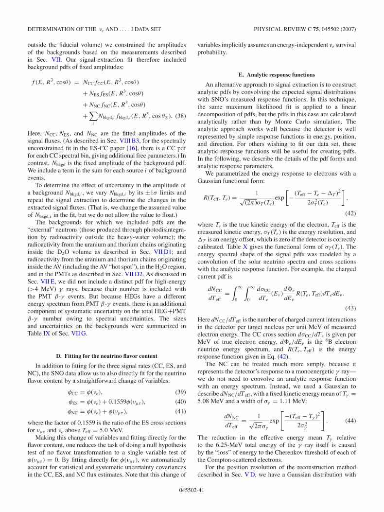
DETERMINATION OF THE νe AND . . . . I DATA SET PHYSICAL REVIEW C 75, 045502 (2007)
outside the fiducial volume) we constrained the amplitudesof the backgrounds based on the measurements describedin Sec. VII. Our signal-extraction fit therefore includedbackground pdfs of fixed amplitudes:
f (E,R3, cosθ ) = NCCfCC(E,R3, cosθ )
+NESfES(E,R3, cosθ )
+NNCfNC(E,R3, cosθ )
+∑
i
Nbkgd,ifbkgd,i(E,R3, cos θ�). (38)
Here, NCC, NES, and NNC are the fitted amplitudes of thesignal fluxes. (As described in Sec. VIII B3, for the spectrallyunconstrained fit in the ES-CC paper [16], there is a CC pdffor each CC spectral bin, giving additional free parameters.) Incontrast, Nbkgd is the fixed amplitude of the background pdf.We include a term in the sum for each source i of backgroundevents.
To determine the effect of uncertainty in the amplitude ofa background Nbkgd,i , we vary Nbkgd,i by its ±1σ limits andrepeat the signal extraction to determine the changes in theextracted signal fluxes. (That is, we change the assumed valueof Nbkgd,i in the fit, but we do not allow the value to float.)
The backgrounds for which we included pdfs are the“external” neutrons (those produced through photodisintegra-tion by radioactivity outside the heavy-water volume); theradioactivity from the uranium and thorium chains originatinginside the D2O volume as described in Sec. VII D1; andradioactivity from the uranium and thorium chains originatinginside the AV (including the AV “hot spot”), in the H2O region,and in the PMTs as described in Sec. VII D2. As discussed inSec. VII E, we did not include a distinct pdf for high-energy(>4 MeV) γ rays, because their number is included withthe PMT β-γ events. But because HEGs have a differentenergy spectrum from PMT β-γ events, there is an additionalcomponent of systematic uncertainty on the total HEG+PMTβ-γ number owing to spectral uncertainties. The sizesand uncertainties on the backgrounds were summarized inTable IX of Sec. VII G.
D. Fitting for the neutrino flavor content
In addition to fitting for the three signal rates (CC, ES, andNC), the SNO data allow us to also directly fit for the neutrinoflavor content by a straightforward change of variables:
φCC = φ(νe), (39)
φES = φ(νe) + 0.1559φ(νµτ ), (40)
φNC = φ(νe) + φ(νµτ ), (41)
where the factor of 0.1559 is the ratio of the ES cross sectionsfor νµτ and νe above Teff = 5.0 MeV.
Making this change of variables and fitting directly for theflavor content, one reduces the task of doing a null hypothesistest of no flavor transformation to a single variable test ofφ(νµτ ) = 0. By fitting directly for φ(νµτ ), we automaticallyaccount for statistical and systematic uncertainty covariancesin the CC, ES, and NC flux estimates. Note that this change of
variables implicitly assumes an energy-independent νe survivalprobability.
E. Analytic response functions
An alternative approach to signal extraction is to constructanalytic pdfs by convolving the expected signal distributionswith SNO’s measured response functions. In this technique,the same maximum likelihood fit is applied to a lineardecomposition of pdfs, but the pdfs in this case are calculatedanalytically rather than by Monte Carlo simulation. Theanalytic approach works well because the detector is wellrepresented by simple response functions in energy, position,and direction. For others wishing to fit our data set, theseanalytic response functions will be useful for creating pdfs.In the following, we describe the details of the pdf forms andanalytic response parameters.
We parametrized the energy response to electrons with aGaussian functional form:
R(Teff, Te) = 1√(2π )σT (Te)
exp
[− (Teff − Te − �T )2
2σ 2T (Te)
],
(42)
where Te is the true kinetic energy of the electron, Teff is themeasured kinetic energy, σT (Te) is the energy resolution, and�T is an energy offset, which is zero if the detector is correctlycalibrated. Table X gives the functional form of σT (Te). Theenergy spectral shape of the signal pdfs was modeled by aconvolution of the solar neutrino spectra and cross sectionswith the analytic response function. For example, the chargedcurrent pdf is
dNCC
dTeff=
∫ ∞
0
∫ ∞
0
dσCC
dTe
(Eν)d�e
dEν
R(Te, Teff)dTedEν .
(43)
Here dNCC/dTeff is the number of charged current interactionsin the detector per target nucleus per unit MeV of measuredelectron energy. The CC cross section dσCC/dTe is given perMeV of true electron energy, d�e/dEν is the 8B electronneutrino energy spectrum, and R(Te, Teff) is the energyresponse function given in Eq. (42).
The NC can be treated much more simply, because itrepresents the detector’s response to a monoenergetic γ ray—we do not need to convolve an analytic response functionwith an energy spectrum. Instead, we used a Gaussian todescribe dNNC/dTeff , with a fixed kinetic energy mean of Tγ =5.08 MeV and a width of σγ = 1.11 MeV:
dNNC
dTeff= 1√
2πσγ
exp
[−(Teff − Tγ )2
2σ 2γ
]. (44)
The reduction in the effective energy mean Tγ relativeto the 6.25-MeV total energy of the γ ray itself is causedby the “loss” of energy to the Cherenkov threshold of each ofthe Compton-scattered electrons.
For the position resolution of the reconstruction methoddescribed in Sec. V D, we have a Gaussian distribution with
045502-41
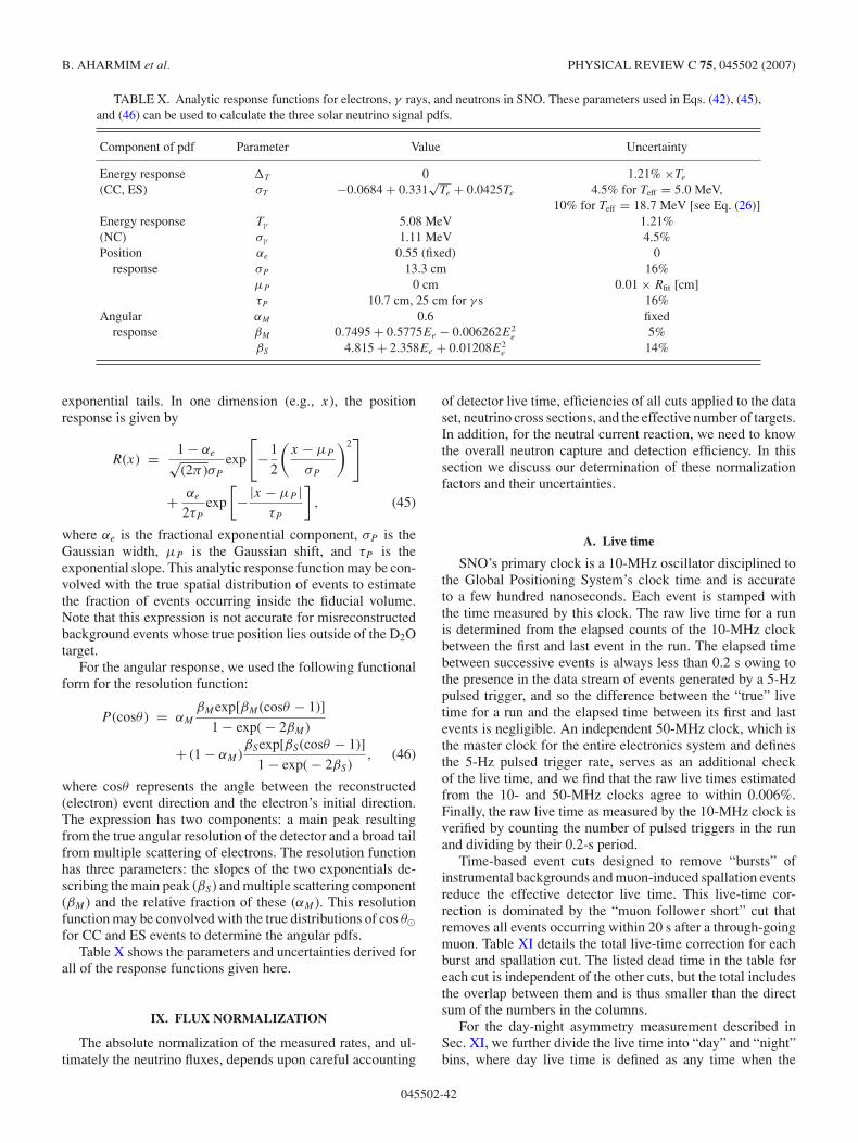
B. AHARMIM et al. PHYSICAL REVIEW C 75, 045502 (2007)
TABLE X. Analytic response functions for electrons, γ rays, and neutrons in SNO. These parameters used in Eqs. (42), (45),and (46) can be used to calculate the three solar neutrino signal pdfs.
Component of pdf Parameter Value Uncertainty
Energy response �T 0 1.21% ×Te
(CC, ES) σT −0.0684 + 0.331√
Te + 0.0425Te 4.5% for Teff = 5.0 MeV,10% for Teff = 18.7 MeV [see Eq. (26)]
Energy response Tγ 5.08 MeV 1.21%(NC) σγ 1.11 MeV 4.5%Position αe 0.55 (fixed) 0
response σP 13.3 cm 16%µP 0 cm 0.01 × Rfit [cm]τP 10.7 cm, 25 cm for γ s 16%
Angular αM 0.6 fixedresponse βM 0.7495 + 0.5775Ee − 0.006262E2
e 5%βS 4.815 + 2.358Ee + 0.01208E2
e 14%
exponential tails. In one dimension (e.g., x), the positionresponse is given by
R(x) = 1 − αe√(2π )σP
exp
[−1
2
(x − µP
σP
)2]
+ αe
2τP
exp
[−|x − µP |
τP
], (45)
where αe is the fractional exponential component, σP is theGaussian width, µP is the Gaussian shift, and τP is theexponential slope. This analytic response function may be con-volved with the true spatial distribution of events to estimatethe fraction of events occurring inside the fiducial volume.Note that this expression is not accurate for misreconstructedbackground events whose true position lies outside of the D2Otarget.
For the angular response, we used the following functionalform for the resolution function:
P (cosθ ) = αM
βMexp[βM (cosθ − 1)]
1 − exp( − 2βM )
+ (1 − αM )βSexp[βS(cosθ − 1)]
1 − exp( − 2βS), (46)
where cosθ represents the angle between the reconstructed(electron) event direction and the electron’s initial direction.The expression has two components: a main peak resultingfrom the true angular resolution of the detector and a broad tailfrom multiple scattering of electrons. The resolution functionhas three parameters: the slopes of the two exponentials de-scribing the main peak (βS) and multiple scattering component(βM ) and the relative fraction of these (αM ). This resolutionfunction may be convolved with the true distributions of cos θ�for CC and ES events to determine the angular pdfs.
Table X shows the parameters and uncertainties derived forall of the response functions given here.
IX. FLUX NORMALIZATION
The absolute normalization of the measured rates, and ul-timately the neutrino fluxes, depends upon careful accounting
of detector live time, efficiencies of all cuts applied to the dataset, neutrino cross sections, and the effective number of targets.In addition, for the neutral current reaction, we need to knowthe overall neutron capture and detection efficiency. In thissection we discuss our determination of these normalizationfactors and their uncertainties.
A. Live time
SNO’s primary clock is a 10-MHz oscillator disciplined tothe Global Positioning System’s clock time and is accurateto a few hundred nanoseconds. Each event is stamped withthe time measured by this clock. The raw live time for a runis determined from the elapsed counts of the 10-MHz clockbetween the first and last event in the run. The elapsed timebetween successive events is always less than 0.2 s owing tothe presence in the data stream of events generated by a 5-Hzpulsed trigger, and so the difference between the “true” livetime for a run and the elapsed time between its first and lastevents is negligible. An independent 50-MHz clock, which isthe master clock for the entire electronics system and definesthe 5-Hz pulsed trigger rate, serves as an additional checkof the live time, and we find that the raw live times estimatedfrom the 10- and 50-MHz clocks agree to within 0.006%.Finally, the raw live time as measured by the 10-MHz clock isverified by counting the number of pulsed triggers in the runand dividing by their 0.2-s period.
Time-based event cuts designed to remove “bursts” ofinstrumental backgrounds and muon-induced spallation eventsreduce the effective detector live time. This live-time cor-rection is dominated by the “muon follower short” cut thatremoves all events occurring within 20 s after a through-goingmuon. Table XI details the total live-time correction for eachburst and spallation cut. The listed dead time in the table foreach cut is independent of the other cuts, but the total includesthe overlap between them and is thus smaller than the directsum of the numbers in the columns.
For the day-night asymmetry measurement described inSec. XI, we further divide the live time into “day” and “night”bins, where day live time is defined as any time when the
045502-42
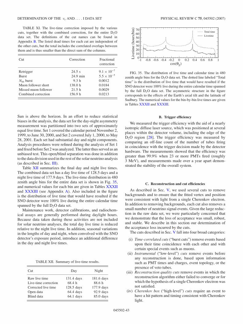
DETERMINATION OF THE νe AND . . . . I DATA SET PHYSICAL REVIEW C 75, 045502 (2007)
TABLE XI. The live-time correction imposed by the variouscuts, together with the combined correction, for the entire D2Odata set. The definitions of the cut names can be found inAppendix B. The listed dead times for each cut are independent ofthe other cuts, but the total includes the correlated overlaps betweenthem and is thus smaller than the direct sum of the columns.
Cut Correction Fractionalcorrection
Retrigger 24.5 s 9.1 × 10⁻⁷
Burst 24.9 min 5.5 × 10⁻⁵
Nhit burst 9.3 h 0.0012Muon follower short 138.0 h 0.0184Missed muon follower 21.5 h 0.0029Combined correction 156.9 h 0.0213
Sun is above the horizon. In an effort to reduce statisticalbiases in the analysis, the data set for the day-night asymmetrymeasurement was partitioned into two sets of approximatelyequal live time. Set 1 covered the calendar period November 2,1999, to June 30, 2000, and Set 2 covered July 1, 2000, to May28, 2001. Each set had substantial day and night components.Analysis procedures were refined during the analysis of Set 1and fixed before Set 2 was analyzed. The latter thus served as anunbiased test. This open/blind separation was done in additionto the data division used in the rest of the solar neutrino analysis(as described in Sec. III).
Table XII summarizes the final day and night live times.The combined data set has a day live time of 128.5 days and anight live time of 177.9 days. The live-time distribution in 480zenith angle bins for the entire data set is shown in Fig. 35,and numerical values for each bin are given in Tables XXXIIand XXXIII (see Appendix A). Also included in the figureis the distribution of live time that would have resulted if theSNO detector were 100% live during the entire calendar timespanned by the full D2O data set.
Maintenance work, detector calibrations, and radiochem-ical assays are generally performed during daylight hours.Because data taken during these activities are not includedfor solar neutrino analyses, the total day live time is reducedrelative to the night live time. In addition, seasonal variationsin the lengths of day and night, when convolved with the SNOdetector’s exposure period, introduce an additional differencein the day and night live times.
TABLE XII. Summary of live-time results.
Cut Day Night
Raw live time 131.4 days 181.6 daysLive-time correction 68.4 h 88.6 hCorrected live time 128.5 days 177.9 daysOpen data 64.4 days 92.9 daysBlind data 64.1 days 85.0 days
cos(θZ)
Liv
etim
e (h
ours
/bin
)
Total time
Livetime
010203040506070
-1 -0.8 -0.6 -0.4 -0.2 0 0.2 0.4 0.6 0.8 1
FIG. 35. The distribution of live time and calendar time in 480zenith angle bins for the D2O data set. The dotted line labeled “Totaltime” is the distribution of live time that would have resulted if theSNO detector were 100% live during the entire calendar time spannedby the full D2O data set. The asymmetric structure in the figurecorresponds to the effects of the Earth’s axial tilt and the latitude ofSudbury. The numerical values for the bin-by-bin live times are givenin Tables XXXII and XXXIII.
B. Trigger efficiency
We measured the trigger efficiency with the aid of a nearlyisotropic diffuse laser source, which was positioned at severalplaces within the detector volume, including the edge of theD2O region [28]. The trigger efficiency was measured bycomparing an off-line count of the number of tubes firingin coincidence with the trigger decision made by the detectorhardware. The measurements showed that the efficiency wasgreater than 99.9% when 23 or more PMTs fired (roughly3 MeV), and measurements made over a year apart demon-strated the stability of the overall system.
C. Reconstruction and cut efficiencies
As described in Sec. V, we used several cuts to removebackgrounds and to ensure that the fitted vertex and positionwere consistent with light from a single Cherenkov electron.In addition to removing backgrounds, each cut also removes asmall number of neutrino signal events. Given the large reduc-tion in the raw data set, we were particularly concerned thatwe demonstrate that the loss of acceptance was small, robust,and stable. We describe in this section our determination ofthe acceptance loss incurred by the cuts.
The cuts described in Sec. V fall into four broad categories:
(i) Time-correlated cuts (“burst cuts”) remove events basedupon their time coincidence with each other and withcertain special events such as muons.
(ii) Instrumental (“low-level”) cuts remove events beforeany reconstruction is done, based upon informationsuch as PMT times and charges, event topology, or thepresence of veto tubes.
(iii) Reconstruction quality cuts remove events in which thereconstruction algorithm either failed to converge or forwhich the hypothesis of a single Cherenkov electron wasnot satisfied.
(iv) Cherenkov box (“high-level”) cuts require an event tohave a hit pattern and timing consistent with Cherenkovlight.
045502-43
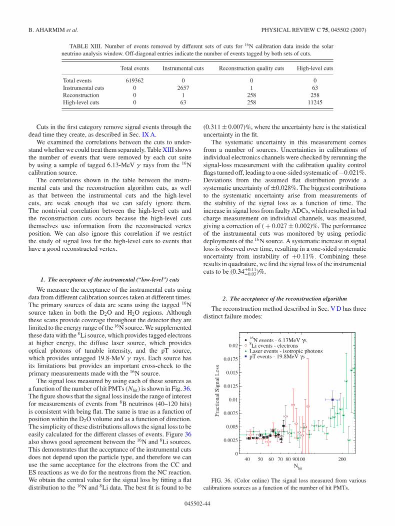
B. AHARMIM et al. PHYSICAL REVIEW C 75, 045502 (2007)
TABLE XIII. Number of events removed by different sets of cuts for 16N calibration data inside the solarneutrino analysis window. Off-diagonal entries indicate the number of events tagged by both sets of cuts.
Total events Instrumental cuts Reconstruction quality cuts High-level cuts
Total events 619362 0 0 0Instrumental cuts 0 2657 1 63Reconstruction 0 1 258 258High-level cuts 0 63 258 11245
Cuts in the first category remove signal events through thedead time they create, as described in Sec. IX A.
We examined the correlations between the cuts to under-stand whether we could treat them separately. Table XIII showsthe number of events that were removed by each cut suiteby using a sample of tagged 6.13-MeV γ rays from the 16Ncalibration source.
The correlations shown in the table between the instru-mental cuts and the reconstruction algorithm cuts, as wellas that between the instrumental cuts and the high-levelcuts, are weak enough that we can safely ignore them.The nontrivial correlation between the high-level cuts andthe reconstruction cuts occurs because the high-level cutsthemselves use information from the reconstructed vertexposition. We can also ignore this correlation if we restrictthe study of signal loss for the high-level cuts to events thathave a good reconstructed vertex.
1. The acceptance of the instrumental (“low-level”) cuts
We measure the acceptance of the instrumental cuts usingdata from different calibration sources taken at different times.The primary sources of data are scans using the tagged 16Nsource taken in both the D2O and H2O regions. Althoughthese scans provide coverage throughout the detector they arelimited to the energy range of the 16N source. We supplementedthese data with the 8Li source, which provides tagged electronsat higher energy, the diffuse laser source, which providesoptical photons of tunable intensity, and the pT source,which provides untagged 19.8-MeV γ rays. Each source hasits limitations but provides an important cross-check to theprimary measurements made with the 16N source.
The signal loss measured by using each of these sources asa function of the number of hit PMTs (Nhit) is shown in Fig. 36.The figure shows that the signal loss inside the range of interestfor measurements of events from 8B neutrinos (40–120 hits)is consistent with being flat. The same is true as a function ofposition within the D2O volume and as a function of direction.The simplicity of these distributions allows the signal loss to beeasily calculated for the different classes of events. Figure 36also shows good agreement between the 16N and 8Li sources.This demonstrates that the acceptance of the instrumental cutsdoes not depend upon the particle type, and therefore we canuse the same acceptance for the electrons from the CC andES reactions as we do for the neutrons from the NC reaction.We obtain the central value for the signal loss by fitting a flatdistribution to the 16N and 8Li data. The best fit is found to be
(0.311 ± 0.007)%, where the uncertainty here is the statisticaluncertainty in the fit.
The systematic uncertainty in this measurement comesfrom a number of sources. Uncertainties in calibrations ofindividual electronics channels were checked by rerunning thesignal-loss measurement with the calibration quality controlflags turned off, leading to a one-sided systematic of −0.021%.Deviations from the assumed flat distribution provide asystematic uncertainty of ±0.028%. The biggest contributionsto the systematic uncertainty arise from measurements ofthe stability of the signal loss as a function of time. Theincrease in signal loss from faulty ADCs, which resulted in badcharge measurement on individual channels, was measured,giving a correction of ( + 0.027 ± 0.002)%. The performanceof the instrumental cuts was monitored by using periodicdeployments of the 16N source. A systematic increase in signalloss is observed over time, resulting in a one-sided systematicuncertainty from instability of +0.11%. Combining theseresults in quadrature, we find the signal loss of the instrumentalcuts to be (0.34+0.11
−0.03)%.
2. The acceptance of the reconstruction algorithm
The reconstruction method described in Sec. V D has threedistinct failure modes:
16N events - 6.13MeV γs8Li events - electronsLaser events - isotropic photonspT events - 19.8MeV γs
Nhit
Frac
tiona
l Sig
nal L
oss
0
0.0025
0.005
0.0075
0.01
0.0125
0.015
0.0175
0.02
40 50 60 70 80 90100 200
FIG. 36. (Color online) The signal loss measured from variouscalibrations sources as a function of the number of hit PMTs.
045502-44
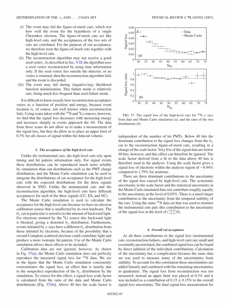
DETERMINATION OF THE νe AND . . . . I DATA SET PHYSICAL REVIEW C 75, 045502 (2007)
(i) The event may fail the figure-of-merit cuts, which testhow well the event fits the hypothesis of a singleCherenkov electron. The figure-of-merit cuts act likehigh-level cuts, and the acceptances of the two sets ofcuts are correlated. For the purpose of cut acceptance,we therefore treat the figure-of-merit cuts together withthe high-level cuts.
(ii) The reconstruction algorithm may not receive a goodseed vertex. As described in Sec. V D, the algorithm usesa seed vertex reconstructed by using time informationonly. If the seed vertex lies outside the detector, or novertex is returned, then the reconstruction algorithm failsand the event is discarded.
(iii) The event may fail during (negative-log) likelihoodfunction minimization. This failure mode is relativelyrare, being much less frequent than seed failure mode.
It is difficult to know exactly how reconstruction acceptancevaries as a function of position and energy, because eventlocation is, of course, not well known when reconstructionfails. Using scans taken with the 16N and 8Li sources, however,we find that the signal loss decreases with increasing energyand increases sharply as events approach the AV. The datafrom these scans do not allow us to make a measurement ofthe signal loss, but they do allow us to place an upper limit of0.3% for all classes of signal within the fiducial volume.
3. The acceptance of the high-level cuts
Unlike the instrumental cuts, the high-level cuts rely upontiming and hit pattern information only. For signal eventsthese distributions can be reproduced much more reliablyby simulation than can distributions such as the PMT chargedistribution, and the Monte Carlo simulation can be used tointegrate the distributions of cut acceptance for the high-levelcuts with the expected distributions for the three signalsobserved in SNO. Unlike the instrumental cuts and thereconstruction algorithm, the high-level cuts have differentacceptances for each of the three signals (CC, ES, and NC).
The Monte Carlo simulation is used to calculate theacceptance for the high-level cuts because we have no electroncalibration source that is unaffected by its own hardware. Theθij cut in particular is sensitive to the amount of backward light.For electrons emitted by the 8Li source this backward lightis blocked, giving a distorted θij distribution. Furthermore,events initiated by γ rays have a different θij distribution fromthose initiated by electrons, because of the possibility that asecond Compton-scattered electron could contribute light andproduce a more isotropic hit pattern. Use of the Monte Carlosimulation allows these effects to be included.
Calibration data are not ignored, however. As shownin Fig. 37(a), the Monte Carlo simulation does not perfectlyreproduce the measured signal loss for 16N data. We seein the figure that the Monte Carlo simulation consistentlyoverestimates the signal loss, an effect that is mainly dueto the nonperfect reproduction of the θij distribution by thesimulation. To correct for this effect, a signal-loss scale factoris calculated from the ratio of the data and Monte Carlodistributions [Fig. 37(b)]. Above 40 hits the scale factor is
0
0.01
0.02
0.03
0.04
0.05
0.06
30 35 40 45 50 55 60 65 70 75
(a)
Nhit
Sign
al lo
ss
DataMonte Carlo
(b)
Nhit
Sign
al lo
ss r
atio
0
0.2
0.4
0.6
0.8
1
30 35 40 45 50 55 60 65 70 75
FIG. 37. The signal loss of the high-level cuts for 16N γ raysfrom data and Monte Carlo simulation (a), and the ratio of the twodistributions (b).
independent of the number of hit PMTs. Below 40 hits thedominant contribution to the signal loss changes from the θij
cut to the reconstruction figure-of-merit cuts, resulting in achange of the scale factor. Very few of the signal data are below40 hits, however, and this effect can therefore be ignored. Thescale factor derived from a fit to the data above 40 hits istherefore used in the analysis. Using the scale factor gives asignal loss of electrons within the analysis region of ∼0.94%compared to 1.79% for neutrons.
There are three dominant contributions to the uncertaintyof the signal loss caused by high-level cuts. The systematicuncertainty in the scale factor and the statistical uncertainty inthe Monte Carlo simulated data sets contribute roughly equallyto the uncertainty at the level of 0.05%. There is a much largercontribution to the uncertainty from the temporal stability ofthe cuts. Using the same 16N data set that was used to monitorthe instrumental cuts puts this contribution to the uncertaintyof the signal loss at the level of (+0.25
−0.11)%.
4. Overall cut acceptance
As all three contributions to the signal loss (instrumentalcuts, reconstruction failures, and high-level cuts) are small andessentially uncorrelated, the combined signal loss can be foundby direct addition of the individual contributions. Calculationof the uncertainty has a complication because the same dataset was used to measure many of the uncertainties fromstability. To account for this correlation these uncertainties areadded linearly and combined with the remaining uncertaintiesin quadrature. The signal loss from reconstruction was notmeasured; instead an upper limit was placed at 0.3% and itwas included as a contribution of 0.15 ± 0.15% to the overallsignal-loss uncertainty. The final signal-loss measurement for
045502-45
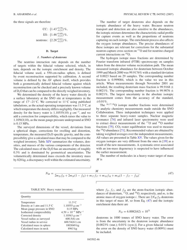
B. AHARMIM et al. PHYSICAL REVIEW C 75, 045502 (2007)
the three signals are therefore
CC:(1.43+0.39
−0.21
)%,
ES:(1.46+0.40
−0.21
)%,
neutrons:(2.28+0.41
−0.23
)%.
D. Target
1. Numbers of deuterons
The neutrino interaction rate depends on the numberof targets within the fiducial volume selected, which, inturn, depends on the isotopic enrichment and density. Thefiducial volume used, a 550-cm-radius sphere, is definedby event reconstruction supported by calibration. A secondvolume is defined by the AV sphere itself, which providesboth a geometrically defined fiducial volume against whichreconstruction can be checked and a precisely known volumeof D2O that can be compared to the directly weighed inventory.
We determined the density of the heavy water directly ina surface laboratory at the SNO site at temperatures in therange of 17◦–21◦C. We corrected to 11◦C using publishedtabulations, as the actual operating temperature was 11.5◦C, atwhich temperature the density differs negligibly. Our measureddensity for the heavy water is 1.10555(10) g cm−3, and weadd a correction for compressibility, which raises the value to1.10563(10), as the mean gauge pressure underground at SNOis 0.15 MPa.
The surveyed dimensions of the vessel, deviations froma spherical shape, corrections for swelling and distortion,temperature, the measured D2O specific gravity, and the com-pressibility give a calculated mass that may be compared to theweighed inventory. Table XIV summarizes the volumes, den-sities, and masses of the various components of the detector.The calculated mass of the D2O has an uncertainty of roughly0.3% and is dominated by geometrical uncertainties. Thevolumetrically determined mass exceeds the inventory massby 828 kg, a discrepancy well within the estimated uncertainty.
The number of target deuterons also depends on theisotopic abundance of the heavy water. Because neutrontransport and detection are also sensitive to the abundances,the isotopic mixture determines the characteristic radial profilefor capture events as well as the proportions of neutronscapturing on each isotope. The enrichment process also affectsthe oxygen isotope abundances. The precise abundances ofthese isotopes are relevant for corrections for the substantialneutron-capture cross section on 17O and for neutrino chargedcurrent interactions on 18O.
The hydrogen isotope mass fractions are determined byFourier transform infrared (FTIR) spectroscopy on samplestaken from the detector volume recirculation path. The meanmeasured isotopic abundance for deuterium between October1999 and March 2000 was 99.9176% with a standard deviationof 0.0023 based on 29 samples. The corresponding numberfraction is 0.999084, which is the value we use in thisarticle. When measurements through November 2001 areincluded, the resulting deuterium mass fraction is 99.9168 ±0.0021%. The corresponding number fraction is 99.9076 ±0.0021%. The largest uncertainty in the absolute isotopicmeasurement comes from the accuracy of the standard,±0.01%.
The 16,17,18O isotope number fractions were determinedby analytic chemistry measurements made outside the SNOCollaboration. Three independent techniques were appliedto three separate heavy-water samples. Nuclear magneticresonance [74] and infrared laser spectrometry were usedto extract direct measurements of the 17O and 18O numberfractions [75]. CO2-water equilibration was used to measurethe 18O abundance [71]. Recommended values are obtained bytaking weighted averages over the independent measurements.All values are presented in Table XV. The values given for theoxygen isotopes are very different from the ones in [19] as aresult of the new measurements. A systematic error associatedwith an ion-mass degeneracy is suspected to have influencedthe earlier measurement.
The number of molecules in a heavy-water target of massM is
NM = M
2mDfD + 2mH (1 − fD) + m17f17 + m18f18 + m16(1 − f17 − f18), (47)
TABLE XIV. Heavy water inventory.
Quantity
Temperature 11.5◦CDensity at 1 atm and 11.5◦C 1.10555 g cm−3
Mean gauge pressure in SNO 0.15 MPaIsothermal compressibility 4.59 × 10⁻⁴ MPa−1
Corrected density 1.10563 g cm−3
Vessel radius as surveyed 600.5(6) cmVessel radius in service 600.54(61) cmCalculated mass in sphere 1003049 kgCalculated mass in neck 8963 kg
where fD, f17, and f18 are the atom-fraction isotopic abun-dances of deuterium, 17O, and 18O, respectively, and mi is theatomic mass of oxygen isotope i. There are 2NMfD deuteronsin this target of mass M , so from Eq. (47) and the isotopicenrichment data there are
ND = 6.0082(62) × 1031
deuterons in 1000 tonnes of SNO heavy water. The erroris from the uncertainty in the deuteron isotopic abundance[0.0023% (stat.); 0.01% (syst.)]. For a given fiducial volumethe error on the density of SNO heavy water (0.009%) mustbe included.
045502-46
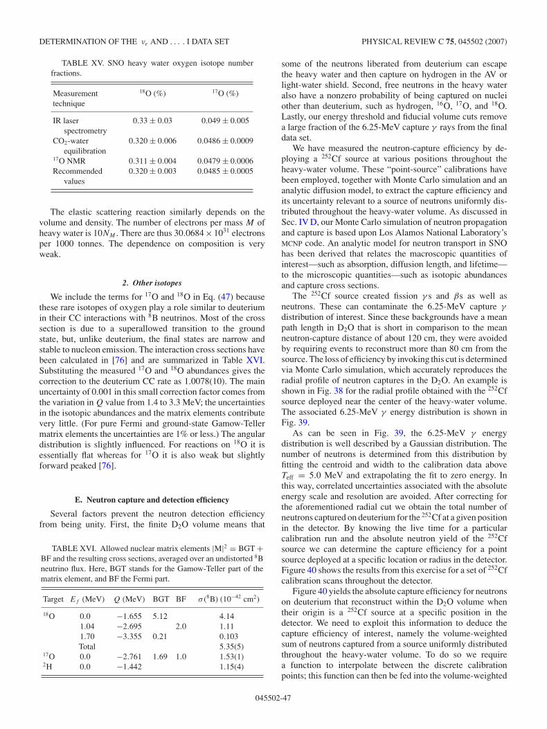
DETERMINATION OF THE νe AND . . . . I DATA SET PHYSICAL REVIEW C 75, 045502 (2007)
TABLE XV. SNO heavy water oxygen isotope numberfractions.
Measurement 18O (%) 17O (%)technique
IR laser 0.33 ± 0.03 0.049 ± 0.005spectrometry
CO2-water 0.320 ± 0.006 0.0486 ± 0.0009equilibration
17O NMR 0.311 ± 0.004 0.0479 ± 0.0006Recommended 0.320 ± 0.003 0.0485 ± 0.0005
values
The elastic scattering reaction similarly depends on thevolume and density. The number of electrons per mass M ofheavy water is 10NM . There are thus 30.0684×1031 electronsper 1000 tonnes. The dependence on composition is veryweak.
2. Other isotopes
We include the terms for 17O and 18O in Eq. (47) becausethese rare isotopes of oxygen play a role similar to deuteriumin their CC interactions with 8B neutrinos. Most of the crosssection is due to a superallowed transition to the groundstate, but, unlike deuterium, the final states are narrow andstable to nucleon emission. The interaction cross sections havebeen calculated in [76] and are summarized in Table XVI.Substituting the measured 17O and 18O abundances gives thecorrection to the deuterium CC rate as 1.0078(10). The mainuncertainty of 0.001 in this small correction factor comes fromthe variation in Q value from 1.4 to 3.3 MeV; the uncertaintiesin the isotopic abundances and the matrix elements contributevery little. (For pure Fermi and ground-state Gamow-Tellermatrix elements the uncertainties are 1% or less.) The angulardistribution is slightly influenced. For reactions on 18O it isessentially flat whereas for 17O it is also weak but slightlyforward peaked [76].
E. Neutron capture and detection efficiency
Several factors prevent the neutron detection efficiencyfrom being unity. First, the finite D2O volume means that
TABLE XVI. Allowed nuclear matrix elements |M|2 = BGT +BF and the resulting cross sections, averaged over an undistorted 8Bneutrino flux. Here, BGT stands for the Gamow-Teller part of thematrix element, and BF the Fermi part.
Target Ef (MeV) Q (MeV) BGT BF σ (8B) (10−42 cm2)
18O 0.0 −1.655 5.12 4.141.04 −2.695 2.0 1.111.70 −3.355 0.21 0.103Total 5.35(5)
17O 0.0 −2.761 1.69 1.0 1.53(1)2H 0.0 −1.442 1.15(4)
some of the neutrons liberated from deuterium can escapethe heavy water and then capture on hydrogen in the AV orlight-water shield. Second, free neutrons in the heavy wateralso have a nonzero probability of being captured on nucleiother than deuterium, such as hydrogen, 16O, 17O, and 18O.Lastly, our energy threshold and fiducial volume cuts removea large fraction of the 6.25-MeV capture γ rays from the finaldata set.
We have measured the neutron-capture efficiency by de-ploying a 252Cf source at various positions throughout theheavy-water volume. These “point-source” calibrations havebeen employed, together with Monte Carlo simulation and ananalytic diffusion model, to extract the capture efficiency andits uncertainty relevant to a source of neutrons uniformly dis-tributed throughout the heavy-water volume. As discussed inSec. IV D, our Monte Carlo simulation of neutron propagationand capture is based upon Los Alamos National Laboratory’sMCNP code. An analytic model for neutron transport in SNOhas been derived that relates the macroscopic quantities ofinterest—such as absorption, diffusion length, and lifetime—to the microscopic quantities—such as isotopic abundancesand capture cross sections.
The 252Cf source created fission γ s and βs as well asneutrons. These can contaminate the 6.25-MeV capture γ
distribution of interest. Since these backgrounds have a meanpath length in D2O that is short in comparison to the meanneutron-capture distance of about 120 cm, they were avoidedby requiring events to reconstruct more than 80 cm from thesource. The loss of efficiency by invoking this cut is determinedvia Monte Carlo simulation, which accurately reproduces theradial profile of neutron captures in the D2O. An example isshown in Fig. 38 for the radial profile obtained with the 252Cfsource deployed near the center of the heavy-water volume.The associated 6.25-MeV γ energy distribution is shown inFig. 39.
As can be seen in Fig. 39, the 6.25-MeV γ energydistribution is well described by a Gaussian distribution. Thenumber of neutrons is determined from this distribution byfitting the centroid and width to the calibration data aboveTeff = 5.0 MeV and extrapolating the fit to zero energy. Inthis way, correlated uncertainties associated with the absoluteenergy scale and resolution are avoided. After correcting forthe aforementioned radial cut we obtain the total number ofneutrons captured on deuterium for the 252Cf at a given positionin the detector. By knowing the live time for a particularcalibration run and the absolute neutron yield of the 252Cfsource we can determine the capture efficiency for a pointsource deployed at a specific location or radius in the detector.Figure 40 shows the results from this exercise for a set of 252Cfcalibration scans throughout the detector.
Figure 40 yields the absolute capture efficiency for neutronson deuterium that reconstruct within the D2O volume whentheir origin is a 252Cf source at a specific position in thedetector. We need to exploit this information to deduce thecapture efficiency of interest, namely the volume-weightedsum of neutrons captured from a source uniformly distributedthroughout the heavy-water volume. To do so we requirea function to interpolate between the discrete calibrationpoints; this function can then be fed into the volume-weighted
045502-47
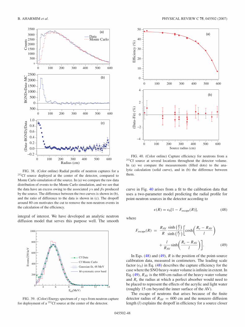
B. AHARMIM et al. PHYSICAL REVIEW C 75, 045502 (2007)
0
0 100 200 300 400 500 600
0 100 200 300 400 500 600
0 100 200 300 400 500 600
Cou
nts
50010001500200025003000
3500
2500
2000
1500
1000
500
500
0
0.0
−0.2
0.2
0.4
0.6
0.8
1.0
BG
ND
=D
ata–
MC
(Dat
a–B
GN
D)/
Dat
a
Radius (cm)
(a)
(c)
(b)
Monte CarloData
FIG. 38. (Color online) Radial profile of neutron captures for a252Cf source deployed at the center of the detector, compared toMonte Carlo simulation of the source. In (a) we compare the raw datadistribution of events to the Monte Carlo simulation, and we see thatthe data have an excess owing to the associated γ s and βs producedby the source. The difference between the two curves is shown in (b),and the ratio of difference to the data is shown in (c). The dropoffaround 80 cm motivates the cut to remove the non-neutron events inthe calculation of the efficiency.
integral of interest. We have developed an analytic neutrondiffusion model that serves this purpose well. The smooth
(MeV)E10 141284 6
Eve
nts/
250
keV
0
200
400
600
800
1000
Cf Data
Cf Monte Carlo
Gaussian fit, 48 MeV
σ1 systematic error band
eff
FIG. 39. (Color) Energy spectrum of γ rays from neutron capturefor deployment of a 252Cf source at the center of the detector.
50
40
30
20
10
0
Eff
icie
ncy
(%)
600
600
500
500
400
400
300
300
200
200
100
100
0
0
−4
−2
0
2
4
(Dat
a–Fi
t) (
%)
Source radius (cm)
(a)
(b)
FIG. 40. (Color online) Capture efficiency for neutrons from a252Cf source at several locations throughout the detector volume.In (a) we compare the measurements (filled dots) to the ana-lytic calculation (solid curve), and in (b) the difference betweenthem.
curve in Fig. 40 arises from a fit to the calibration data thatuses a two-parameter model predicting the radial profile forpoint-neutron sources in the detector according to
ε(R) = ε0[1 − Fescape(R)], (48)
where
Fescape(R) = RAV
R
sinh(
Rl
)sinh
(Re
l
)[cosh
(Re − RAV
l
)
+ l
RAVsinh
(Re − RAV
l
)]. (49)
In Eqs. (48) and (49), R is the position of the point-sourcecalibration data, measured in centimeters. The leading scalefactor (ε0) in Eq. (48) describes the capture efficiency for thecase where the SNO heavy-water volume is infinite in extent. InEq. (49), RAV is the 600-cm radius of the heavy-water volumeand Re the radius at which a perfect absorber would need tobe placed to represent the effects of the acrylic and light water(roughly 15 cm beyond the inner surface of the AV).
The escape of neutrons that arises because of the finitedetector radius of RAV = 600 cm and the nonzero diffusionlength (l) explains the dropoff in efficiency for a source closer
045502-48
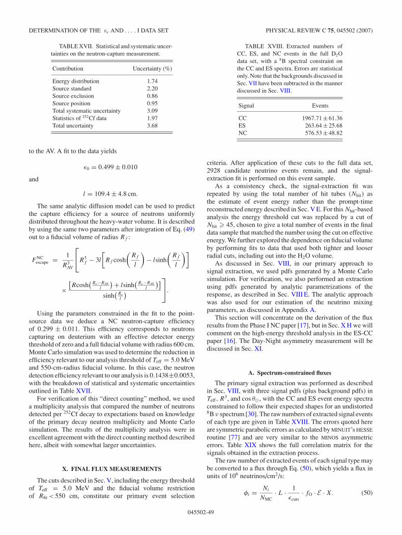
DETERMINATION OF THE νe AND . . . . I DATA SET PHYSICAL REVIEW C 75, 045502 (2007)
TABLE XVII. Statistical and systematic uncer-tainties on the neutron-capture measurement.
Contribution Uncertainty (%)
Energy distribution 1.74Source standard 2.20Source exclusion 0.86Source position 0.95Total systematic uncertainty 3.09Statistics of 252Cf data 1.97Total uncertainty 3.68
to the AV. A fit to the data yields
ε0 = 0.499 ± 0.010
and
l = 109.4 ± 4.8 cm.
The same analytic diffusion model can be used to predictthe capture efficiency for a source of neutrons uniformlydistributed throughout the heavy-water volume. It is describedby using the same two parameters after integration of Eq. (49)out to a fiducial volume of radius Rf :
F NCescape = 1
R3AV
R3
f − 3l
[Rf cosh
(Rf
l
)− lsinh
(Rf
l
)]
×[Rcosh
(Re−RAV
l
) + lsinh(
Re−RAVl
)]sinh
(Re
l
).
Using the parameters constrained in the fit to the point-source data we deduce a NC neutron-capture efficiencyof 0.299 ± 0.011. This efficiency corresponds to neutronscapturing on deuterium with an effective detector energythreshold of zero and a full fiducial volume with radius 600 cm.Monte Carlo simulation was used to determine the reduction inefficiency relevant to our analysis threshold of Teff = 5.0 MeVand 550-cm-radius fiducial volume. In this case, the neutrondetection efficiency relevant to our analysis is 0.1438±0.0053,with the breakdown of statistical and systematic uncertaintiesoutlined in Table XVII.
For verification of this “direct counting” method, we useda multiplicity analysis that compared the number of neutronsdetected per 252Cf decay to expectations based on knowledgeof the primary decay neutron multiplicity and Monte Carlosimulation. The results of the multiplicity analysis were inexcellent agreement with the direct counting method describedhere, albeit with somewhat larger uncertainties.
X. FINAL FLUX MEASUREMENTS
The cuts described in Sec. V, including the energy thresholdof Teff = 5.0 MeV and the fiducial volume restrictionof Rfit < 550 cm, constitute our primary event selection
TABLE XVIII. Extracted numbers ofCC, ES, and NC events in the full D2Odata set, with a 8B spectral constraint onthe CC and ES spectra. Errors are statisticalonly. Note that the backgrounds discussed inSec. VII have been subtracted in the mannerdiscussed in Sec. VIII.
Signal Events
CC 1967.71 ± 61.36ES 263.64 ± 25.68NC 576.53 ± 48.82
criteria. After application of these cuts to the full data set,2928 candidate neutrino events remain, and the signal-extraction fit is performed on this event sample.
As a consistency check, the signal-extraction fit wasrepeated by using the total number of hit tubes (Nhit) asthe estimate of event energy rather than the prompt-timereconstructed energy described in Sec. V E. For this Nhit-basedanalysis the energy threshold cut was replaced by a cut ofNhit � 45, chosen to give a total number of events in the finaldata sample that matched the number using the cut on effectiveenergy. We further explored the dependence on fiducial volumeby performing fits to data that used both tighter and looserradial cuts, including out into the H2O volume.
As discussed in Sec. VIII, in our primary approach tosignal extraction, we used pdfs generated by a Monte Carlosimulation. For verification, we also performed an extractionusing pdfs generated by analytic parametrizations of theresponse, as described in Sec. VIII E. The analytic approachwas also used for our estimation of the neutrino mixingparameters, as discussed in Appendix A.
This section will concentrate on the derivation of the fluxresults from the Phase I NC paper [17], but in Sec. X H we willcomment on the high-energy threshold analysis in the ES-CCpaper [16]. The Day-Night asymmetry measurement will bediscussed in Sec. XI.
A. Spectrum-constrained fluxes
The primary signal extraction was performed as describedin Sec. VIII, with three signal pdfs (plus background pdfs) inTeff, R
3, and cos θ�, with the CC and ES event energy spectraconstrained to follow their expected shapes for an undistorted8B ν spectrum [30]. The raw numbers of extracted signal eventsof each type are given in Table XVIII. The errors quoted hereare symmetric parabolic errors as calculated by MINUIT’s HESSE
routine [77] and are very similar to the MINOS asymmetricerrors. Table XIX shows the full correlation matrix for thesignals obtained in the extraction process.
The raw number of extracted events of each signal type maybe converted to a flux through Eq. (50), which yields a flux inunits of 106 neutrinos/cm2/s:
φi = Ni
NMC· L · 1
εcuts· fO · E · X. (50)
045502-49
B. AHARMIM et al. PHYSICAL REVIEW C 75, 045502 (2007)
TABLE XIX. Statistical correlation matrixamong CC, ES, and NC signals from the signalextraction with a 8B shape constraint.
CC ES NC
CC 1.000 −0.162 −0.520ES −0.162 1.000 −0.105NC −0.520 −0.105 1.000
The various quantities are defined as follows:
Ni : Number of extracted events for a given signal type i,as given in Table XVIII.
NMC: Number of Monte Carlo events inside the signalregion, for a total 8B flux of 1 × 10⁶/cm2/s. The numberof events we generated was 50 times the BPB2000 SSMprediction of 5.15 × 10⁶ νcm−2 s−1 [78].
L: Live-time correction factor. This correction accountsfor detector dead time owing to the imposition of time-correlated cuts (such as those that remove muon followerevents).
εcuts: Acceptance of low- and high-level cuts, as describedin Secs. IX C1 and IX C3, that are not applied to the MonteCarlo simulation.
fO: A correction to the CC flux owing to CC neutrinointeractions on 17O and 18O, as described in Sec. IX D2.These interactions are not modeled in the Monte Carlosimulation. This correction is applicable only to the CCflux.
E : Correction for eccentricity of the Earth’s orbit, whichwas not included in the Monte Carlo generation.
X: Minor corrections to the neutrino cross sectionsassumed in the Monte Carlo simulation. For the CC andNC fluxes, this is a combination of the gA correction tothe Butler, Chen, and Kong (BCK) cross section [32], adownward revision of the NSGK cross section [35], andradiative corrections of Kurylov et al. [34]. See Sec. IV Afor further details.
Table XX contains the values of the flux correction factorsused for each signal. With all of these corrections applied, the
extracted signal fluxes are
φCC = 1.76+0.06−0.05 × 106 cm−2s−1,
φES = 2.39+0.24−0.23 × 106 cm−2s−1,
φNC = 5.09+0.44−0.43 × 106 cm−2s−1.
(where only statistical errors are quoted). The physicalinterpretation of the “flux” for each interaction type is thatit is the equivalent flux of 8B νes produced from an undistortedenergy spectrum that would yield the same number of eventsinside the signal region from that interaction as was seen inthe data set.
The inequality of the CC, ES, and NC fluxes providesstrong evidence for a non-νe component to the 8B neutrinoflux. Figure 41 shows the constraints on the flux of νe versusthe combined νµ and ντ fluxes derived from the CC, ES, andNC rates. Together the three rates are inconsistent with thehypothesis that the 8B flux consists solely of νes, but they arealso consistent with an admixture consisting of ∼1/3νe and2/3νµ and/or ντ .
1. Goodness of fit
The signal extraction is done by a maximum likelihoodfit, which does not readily yield an absolute goodness-of-fitparameter. One means of investigating the goodness of fit ofthe signal extraction is to calculate the χ2 of the radial, energy,and angular marginal distributions between the data and thebest-fit sum of the weighted pdfs. This χ2 is defined as
χ2 =bins∑i=1
[RDATA(i) − Rpdfs(i)]2/RDATA, (51)
where RDATA(i) is the number of counts in the ith bin of thedata (R may be a histogram in energy, angle, or radius), andRpdfs(i) is the predicted number of counts in the ith bin, foundby weighting each signal pdf by the number of fitted eventsand summing these renormalized pdfs. This χ2 calculationdoes not account for systematic uncertainties.
Table XXI shows the χ2 values for the fits determined byusing the constraint that the effective kinetic energy spectrumresults from an undistorted 8B shape. In each case the χ2
per degree of freedom is close to one. One must be cautious
TABLE XX. Flux correction factors for converting event totals to fluxes. The final entry (“Total”) is the product of all thecorrections that are applied to the ratio Ni /MC to convert it into a flux in units of 106 neutrinos/cm2/s.
Correction Symbol CC ES NC
Live time Total/Corrected 312.93/306.39 312.93/306.39 312.93/306.39Cut efficiency εcuts 0.986+0.004
−0.002 0.985+0.004−0.002 0.977+0.004
−0.00217O and 18O correction fO 1/1.00793 1 1Eccentricity correction E 1/1.0069 1/1.0069 1/1.0069Cross section correction X 1/1.0162 1.02 1/1.0112Total correction factor 1.0043 1.0500 1.0267Number of events N 1967.71 ± 61.36 263.64 ± 25.68 576.53 ± 48.82MC prediction (for 106νcm−2 s−1) NMC 1120.48 115.83 116.23
045502-50
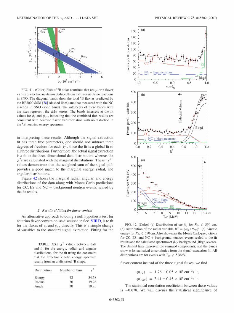
DETERMINATION OF THE νe AND . . . . I DATA SET PHYSICAL REVIEW C 75, 045502 (2007)
0 1 2 3 4 5 60
1
2
3
4
5
6
7
8
)-1 s-2 cm6
(10eφ
)-1
s-2
cm
6 (
10τµφ
SNONCφ
SSMφ
SNOCCφSNO
ESφ
FIG. 41. (Color) Flux of 8B solar neutrinos that are µ or τ flavorvs flux of electron neutrinos deduced from the three neutrino reactionsin SNO. The diagonal bands show the total 8B flux as predicted bythe BP2000 SSM [78] (dashed lines) and that measured with the NCreaction in SNO (solid band). The intercepts of these bands withthe axes represent the ±1σ errors. The bands intersect at the fitvalues for φe and φµτ , indicating that the combined flux results areconsistent with neutrino flavor transformation with no distortion inthe 8B neutrino energy spectrum.
in interpreting these results. Although the signal-extractionfit has three free parameters, one should not subtract threedegrees of freedom for each χ2, since the fit is a global fit toall three distributions. Furthermore, the actual signal extractionis a fit to the three-dimensional data distribution, whereas theχ2s are calculated with the marginal distributions. These “χ2”values demonstrate that the weighted sum of the signal pdfsprovides a good match to the marginal energy, radial, andangular distributions.
Figure 42 shows the marginal radial, angular, and energydistributions of the data along with Monte Carlo predictionsfor CC, ES and NC + background neutron events, scaled bythe fit results.
2. Results of fitting for flavor content
An alternative approach to doing a null hypothesis test forneutrino flavor conversion, as discussed in Sec. VIII D, is to fitfor the fluxes of νe and νµτ directly. This is a simple changeof variables to the standard signal extraction. Fitting for the
TABLE XXI. χ 2 values between dataand fit for the energy, radial, and angulardistributions, for the fit using the constraintthat the effective kinetic energy spectrumresults from an undistorted 8B shape.
Distribution Number of bins χ 2
Energy 42 34.58Radius 30 39.28Angle 30 19.85
-1.0 -0.5 0.0 0.5 1.0
Eve
nts
per
0.05
wid
e bi
n
0
20
40
60
80
100
120
140
160
cos
ESCC
NC + bkgd neutrons
Bkgd
(a)
0.0 0.2 0.4 0.6 0.8 1.0 1.2
Eve
nts
per
0.1
wid
e bi
n
0
100
200
300
400
500
CC
NC + bkgd neutronsES
Bkgd
Fidu
cial
Vol
ume
(b)
3R
5 6 7 8 9 10 11 12 13
Eve
nts
per
500
keV
0
100
200
300
400
500
600
20→
NC + bkgdneutrons
ES
CC
Bkgd
(c)
(MeV)effT
θ
FIG. 42. (Color) (a) Distribution of cos θ� for Rfit � 550 cm.(b) Distribution of the radial variable R3 = (Rfit/RAV)3. (c) Kineticenergy for Rfit � 550 cm. Also shown are the Monte Carlo predictionsfor CC, ES, and NC + background neutron events scaled to the fitresults and the calculated spectrum of β-γ background (Bkgd) events.The dashed lines represent the summed components, and the bandsshow ±1σ statistical uncertainties from the signal-extraction fit. Alldistributions are for events with Teff � 5 MeV.
flavor content instead of the three signal fluxes, we find
φ(νe) = 1.76 ± 0.05 × 106 cm−2s−1,
φ(νµτ ) = 3.41 ± 0.45 × 106 cm−2s−1.
The statistical correlation coefficient between these valuesis −0.678. We will discuss the statistical significance of
045502-51
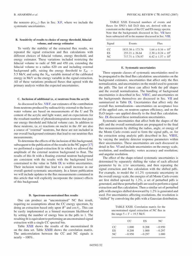
B. AHARMIM et al. PHYSICAL REVIEW C 75, 045502 (2007)
the nonzero φ(νµτ ) flux in Sec. X F, where we include thesystematic uncertainties.
B. Sensitivity of results to choice of energy threshold, fiducialvolume, and energy estimator
To verify the stability of the extracted flux results, werepeated the signal extraction and flux calculations withdifferent choices of fiducial volume, energy threshold, andenergy estimator. These variations included restricting thefiducial volume to radii of 500 and 450 cm, extending thefiducial volume to a radius 620 cm and including externalbackground pdfs, raising the energy threshold to Teff >
5.5 MeV, and using the Nhit variable instead of the calibratedenergy in MeV as the energy variable in the signal extraction.All of these variations produced fluxes that agreed with theprimary analysis within the expected uncertainties.
C. Inclusion of additional (α, n) neutrons from the acrylic
As discussed in Sec. VII F, our estimates of the contributionfrom neutrons produced by radioactivity external to the heavy-water volume are based on measurements of the U and Thcontent of the acrylic and light water, and on expectations forthe resultant number of photodisintegration neutrons that passour energy threshold and fiducial volume cuts. In addition tothese neutrons, (α, n) reactions on nuclei in the AV are alsoa source of “external” neutrons, but these are not included inour overall background estimates that lead to our neutrino fluxmeasurements.
To determine the effects of the inclusion of this background,subsequent to the publication of the results in the NC paper [17]we performed a signal-extraction fit in which we allowed theamplitude of the external neutron background to float. Theresults of this fit with a floating external neutron backgroundare consistent with the results with the background levelconstrained to the value in Table IX to within uncertainties.Their inclusion would thus lead to a small increase in ouroverall quoted systematic uncertainty. In a future publicationwe will include updates to the flux measurements contained inthis article that will explicitly incorporate the (minor) effectsof this background.
D. Spectrum-unconstrained flux results
One can produce an “unconstrained” NC flux result,requiring no assumptions about the CC energy spectrum, bydoing an extraction based only upon R3 and cos θ�. This canbe easily implemented as a binned maximum likelihood fitby setting the number of energy bins in the pdfs to 1. Theresulting fit is equivalent to performing an unconstrained signalextraction with a single CC spectral bin.
Table XXII shows the results of the unconstrained fiton the data set. Table XXIII shows the correlation matrix.The anticorrelation between the CC and NC signals isnearly −100%.
TABLE XXII. Extracted numbers of events andfluxes for SNO’s full D2O data set, derived with noconstraint on the shapes of the CC and ES energy spectra.Note that the backgrounds discussed in Sec. VII havebeen subtracted off in the manner discussed in Sec. VIII.
Signal Events Flux
CC 1833.38 ± 173.76 1.64 ± 0.16 × 10⁶
ES 253.21 ± 26.64 2.30 ± 0.24 × 10⁶
NC 717.71 ± 176.97 6.42 ± 1.57 × 10⁶
E. Systematic uncertainties
Three separate classes of systematic uncertainties need tobe propagated to the final flux calculation: uncertainties on thebackground estimates, uncertainties that affect only the fluxnormalization, and uncertainties on the model used to generatethe pdfs. The last of these can affect both the pdf shapesand the overall normalization. The handling of backgrounduncertainties is described in Sec. VIII C, and uncertainties onthe backgrounds themselves are discussed in Sec. VII andsummarized in Table IX. Uncertainties that affect only theoverall flux normalization—uncertainties on acceptance lossof the applied cuts, on neutron capture efficiency, and on theD2O target—are applied directly to the final flux calculation.Sec. IX discussed these normalization uncertainties.
Systematic uncertainties that affect both the shapes of thepdfs and the overall normalization are propagated to the finalflux measurements by shifting the radius, angle, or energy ofthe Monte Carlo events used to form the signal pdfs, or, forthe extraction using analytic pdfs described in Sec. VIII E,by varying the analytic detector response parameters withintheir uncertainties. These uncertainties are each discussed indetail in Sec. VI and include uncertainties on the energy scale,resolution, and nonlinearity; vertex accuracy and resolution;and angular resolution.
The effect of the shape-related systematic uncertainties isdetermined by separately shifting the value of each affectedparameter by its ±1σ uncertainty, and then repeating thesignal extraction and flux calculation with the shifted pdfs.For example, to model the ±1.2% systematic uncertainty inthe overall energy scale, the energies of all Monte Carlo eventsare first shifted upward by 1.2%, a set of perturbed pdfs isgenerated, and these perturbed pdfs are used to perform a signalextraction and flux calculation. Then a similar set of perturbedpdfs with energies shifted downward by 1.2% is generated andused. For uncertainties affecting resolutions, the resolution is“shifted” by convolving the pdfs with a Gaussian distribution.
TABLE XXIII. Correlation matrix for theunconstrained signal extraction of NC flux inthe range 5 < T < 19.5 MeV.
CC ES NC
CC 1.000 0.208 −0.950ES 0.208 1.000 −0.297NC −0.950 −0.297 1.000
045502-52
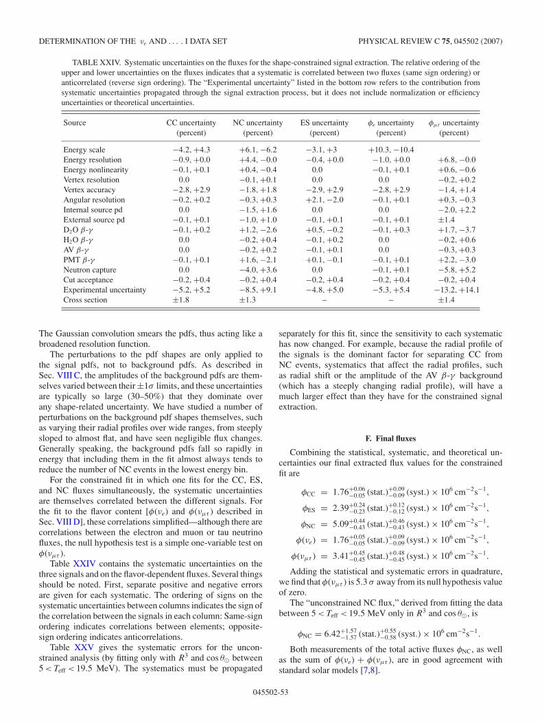
DETERMINATION OF THE νe AND . . . . I DATA SET PHYSICAL REVIEW C 75, 045502 (2007)
TABLE XXIV. Systematic uncertainties on the fluxes for the shape-constrained signal extraction. The relative ordering of theupper and lower uncertainties on the fluxes indicates that a systematic is correlated between two fluxes (same sign ordering) oranticorrelated (reverse sign ordering). The “Experimental uncertainty” listed in the bottom row refers to the contribution fromsystematic uncertainties propagated through the signal extraction process, but it does not include normalization or efficiencyuncertainties or theoretical uncertainties.
Source CC uncertainty NC uncertainty ES uncertainty φe uncertainty φµτ uncertainty(percent) (percent) (percent) (percent) (percent)
Energy scale −4.2, +4.3 +6.1, −6.2 −3.1, +3 +10.3, −10.4Energy resolution −0.9, +0.0 +4.4, −0.0 −0.4, +0.0 −1.0, +0.0 +6.8, −0.0Energy nonlinearity −0.1, +0.1 +0.4, −0.4 0.0 −0.1, +0.1 +0.6, −0.6Vertex resolution 0.0 −0.1, +0.1 0.0 0.0 −0.2, +0.2Vertex accuracy −2.8, +2.9 −1.8, +1.8 −2.9, +2.9 −2.8, +2.9 −1.4, +1.4Angular resolution −0.2, +0.2 −0.3, +0.3 +2.1, −2.0 −0.1, +0.1 +0.3, −0.3Internal source pd 0.0 −1.5, +1.6 0.0 0.0 −2.0, +2.2External source pd −0.1, +0.1 −1.0, +1.0 −0.1, +0.1 −0.1, +0.1 ±1.4D2O β-γ −0.1, +0.2 +1.2, −2.6 +0.5, −0.2 −0.1, +0.3 +1.7, −3.7H2O β-γ 0.0 −0.2, +0.4 −0.1, +0.2 0.0 −0.2, +0.6AV β-γ 0.0 −0.2, +0.2 −0.1, +0.1 0.0 −0.3, +0.3PMT β-γ −0.1, +0.1 +1.6, −2.1 +0.1, −0.1 −0.1, +0.1 +2.2, −3.0Neutron capture 0.0 −4.0, +3.6 0.0 −0.1, +0.1 −5.8, +5.2Cut acceptance −0.2, +0.4 −0.2, +0.4 −0.2, +0.4 −0.2, +0.4 −0.2, +0.4Experimental uncertainty −5.2, +5.2 −8.5, +9.1 −4.8, +5.0 −5.3, +5.4 −13.2, +14.1Cross section ±1.8 ±1.3 – – ±1.4
The Gaussian convolution smears the pdfs, thus acting like abroadened resolution function.
The perturbations to the pdf shapes are only applied tothe signal pdfs, not to background pdfs. As described inSec. VIII C, the amplitudes of the background pdfs are them-selves varied between their ±1σ limits, and these uncertaintiesare typically so large (30–50%) that they dominate overany shape-related uncertainty. We have studied a number ofperturbations on the background pdf shapes themselves, suchas varying their radial profiles over wide ranges, from steeplysloped to almost flat, and have seen negligible flux changes.Generally speaking, the background pdfs fall so rapidly inenergy that including them in the fit almost always tends toreduce the number of NC events in the lowest energy bin.
For the constrained fit in which one fits for the CC, ES,and NC fluxes simultaneously, the systematic uncertaintiesare themselves correlated between the different signals. Forthe fit to the flavor content [φ(νe) and φ(νµτ ) described inSec. VIII D], these correlations simplified—although there arecorrelations between the electron and muon or tau neutrinofluxes, the null hypothesis test is a simple one-variable test onφ(νµτ ).
Table XXIV contains the systematic uncertainties on thethree signals and on the flavor-dependent fluxes. Several thingsshould be noted. First, separate positive and negative errorsare given for each systematic. The ordering of signs on thesystematic uncertainties between columns indicates the sign ofthe correlation between the signals in each column: Same-signordering indicates correlations between elements; opposite-sign ordering indicates anticorrelations.
Table XXV gives the systematic errors for the uncon-strained analysis (by fitting only with R3 and cos θ� between5 < Teff < 19.5 MeV). The systematics must be propagated
separately for this fit, since the sensitivity to each systematichas now changed. For example, because the radial profile ofthe signals is the dominant factor for separating CC fromNC events, systematics that affect the radial profiles, suchas radial shift or the amplitude of the AV β-γ background(which has a steeply changing radial profile), will have amuch larger effect than they have for the constrained signalextraction.
F. Final fluxes
Combining the statistical, systematic, and theoretical un-certainties our final extracted flux values for the constrainedfit are
φCC = 1.76+0.06−0.05 (stat.)+0.09
−0.09 (syst.) × 106 cm−2s−1,
φES = 2.39+0.24−0.23 (stat.)+0.12
−0.12 (syst.) × 106 cm−2s−1,
φNC = 5.09+0.44−0.43 (stat.)+0.46
−0.43 (syst.) × 106 cm−2s−1,
φ(νe) = 1.76+0.05−0.05 (stat.)+0.09
−0.09 (syst.) × 106 cm−2s−1,
φ(νµτ ) = 3.41+0.45−0.45 (stat.)+0.48
−0.45 (syst.) × 106 cm−2s−1.
Adding the statistical and systematic errors in quadrature,we find that φ(νµτ ) is 5.3 σ away from its null hypothesis valueof zero.
The “unconstrained NC flux,” derived from fitting the databetween 5 < Teff < 19.5 MeV only in R3 and cos θ�, is
φNC = 6.42+1.57−1.57 (stat.)+0.55
−0.58 (syst.) × 106 cm−2s−1.
Both measurements of the total active fluxes φNC, as wellas the sum of φ(νe) + φ(νµτ ), are in good agreement withstandard solar models [7,8].
045502-53
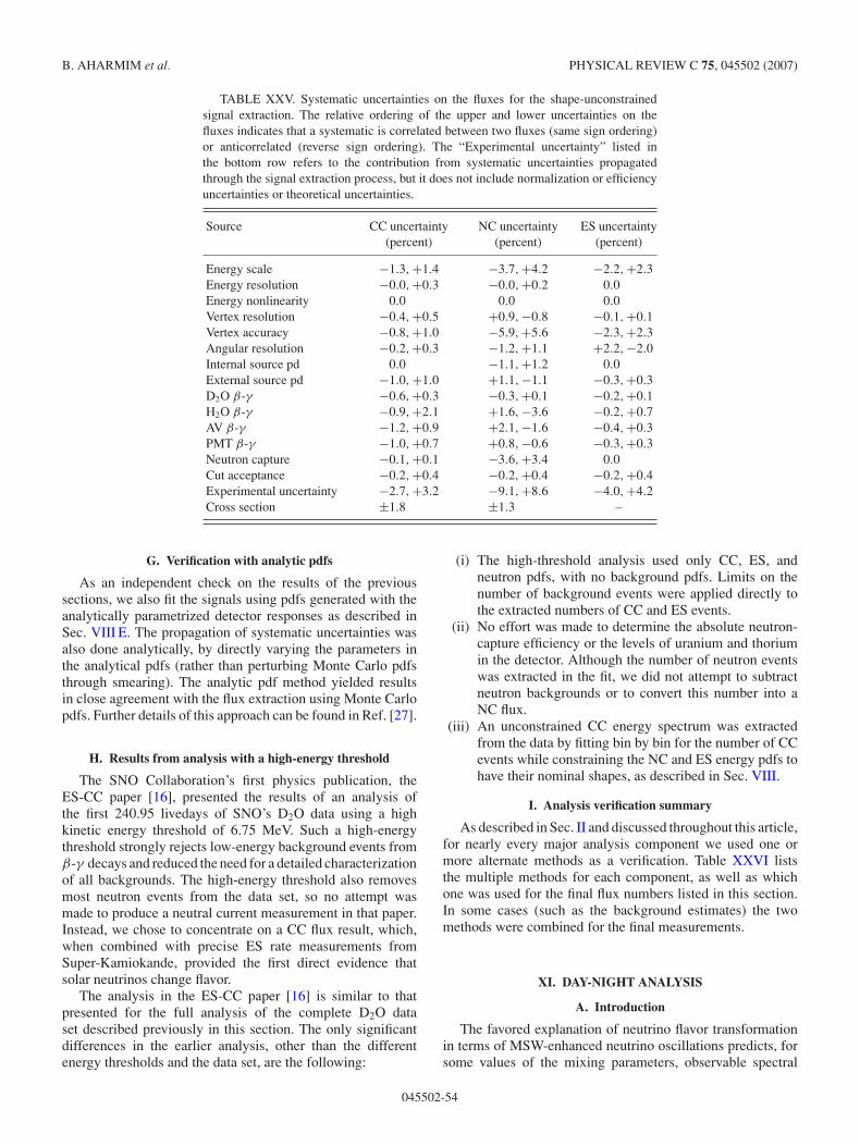
B. AHARMIM et al. PHYSICAL REVIEW C 75, 045502 (2007)
TABLE XXV. Systematic uncertainties on the fluxes for the shape-unconstrainedsignal extraction. The relative ordering of the upper and lower uncertainties on thefluxes indicates that a systematic is correlated between two fluxes (same sign ordering)or anticorrelated (reverse sign ordering). The “Experimental uncertainty” listed inthe bottom row refers to the contribution from systematic uncertainties propagatedthrough the signal extraction process, but it does not include normalization or efficiencyuncertainties or theoretical uncertainties.
Source CC uncertainty NC uncertainty ES uncertainty(percent) (percent) (percent)
Energy scale −1.3, +1.4 −3.7, +4.2 −2.2, +2.3Energy resolution −0.0, +0.3 −0.0, +0.2 0.0Energy nonlinearity 0.0 0.0 0.0Vertex resolution −0.4, +0.5 +0.9, −0.8 −0.1, +0.1Vertex accuracy −0.8, +1.0 −5.9, +5.6 −2.3, +2.3Angular resolution −0.2, +0.3 −1.2, +1.1 +2.2, −2.0Internal source pd 0.0 −1.1, +1.2 0.0External source pd −1.0, +1.0 +1.1, −1.1 −0.3, +0.3D2O β-γ −0.6, +0.3 −0.3, +0.1 −0.2, +0.1H2O β-γ −0.9, +2.1 +1.6, −3.6 −0.2, +0.7AV β-γ −1.2, +0.9 +2.1, −1.6 −0.4, +0.3PMT β-γ −1.0, +0.7 +0.8, −0.6 −0.3, +0.3Neutron capture −0.1, +0.1 −3.6, +3.4 0.0Cut acceptance −0.2, +0.4 −0.2, +0.4 −0.2, +0.4Experimental uncertainty −2.7, +3.2 −9.1, +8.6 −4.0, +4.2Cross section ±1.8 ±1.3 –
G. Verification with analytic pdfs
As an independent check on the results of the previoussections, we also fit the signals using pdfs generated with theanalytically parametrized detector responses as described inSec. VIII E. The propagation of systematic uncertainties wasalso done analytically, by directly varying the parameters inthe analytical pdfs (rather than perturbing Monte Carlo pdfsthrough smearing). The analytic pdf method yielded resultsin close agreement with the flux extraction using Monte Carlopdfs. Further details of this approach can be found in Ref. [27].
H. Results from analysis with a high-energy threshold
The SNO Collaboration’s first physics publication, theES-CC paper [16], presented the results of an analysis ofthe first 240.95 livedays of SNO’s D2O data using a highkinetic energy threshold of 6.75 MeV. Such a high-energythreshold strongly rejects low-energy background events fromβ-γ decays and reduced the need for a detailed characterizationof all backgrounds. The high-energy threshold also removesmost neutron events from the data set, so no attempt wasmade to produce a neutral current measurement in that paper.Instead, we chose to concentrate on a CC flux result, which,when combined with precise ES rate measurements fromSuper-Kamiokande, provided the first direct evidence thatsolar neutrinos change flavor.
The analysis in the ES-CC paper [16] is similar to thatpresented for the full analysis of the complete D2O dataset described previously in this section. The only significantdifferences in the earlier analysis, other than the differentenergy thresholds and the data set, are the following:
(i) The high-threshold analysis used only CC, ES, andneutron pdfs, with no background pdfs. Limits on thenumber of background events were applied directly tothe extracted numbers of CC and ES events.
(ii) No effort was made to determine the absolute neutron-capture efficiency or the levels of uranium and thoriumin the detector. Although the number of neutron eventswas extracted in the fit, we did not attempt to subtractneutron backgrounds or to convert this number into aNC flux.
(iii) An unconstrained CC energy spectrum was extractedfrom the data by fitting bin by bin for the number of CCevents while constraining the NC and ES energy pdfs tohave their nominal shapes, as described in Sec. VIII.
I. Analysis verification summary
As described in Sec. II and discussed throughout this article,for nearly every major analysis component we used one ormore alternate methods as a verification. Table XXVI liststhe multiple methods for each component, as well as whichone was used for the final flux numbers listed in this section.In some cases (such as the background estimates) the twomethods were combined for the final measurements.
XI. DAY-NIGHT ANALYSIS
A. Introduction
The favored explanation of neutrino flavor transformationin terms of MSW-enhanced neutrino oscillations predicts, forsome values of the mixing parameters, observable spectral
045502-54
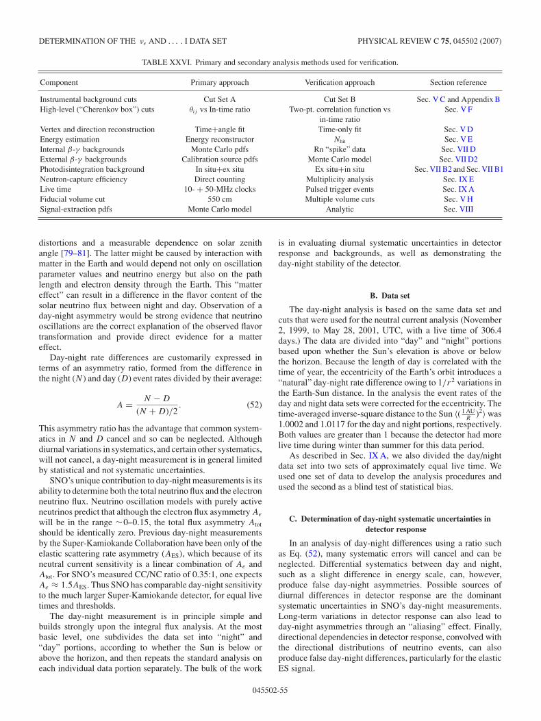
DETERMINATION OF THE νe AND . . . . I DATA SET PHYSICAL REVIEW C 75, 045502 (2007)
TABLE XXVI. Primary and secondary analysis methods used for verification.
Component Primary approach Verification approach Section reference
Instrumental background cuts Cut Set A Cut Set B Sec. V C and Appendix BHigh-level (“Cherenkov box”) cuts θij vs In-time ratio Two-pt. correlation function vs
in-time ratioSec. V F
Vertex and direction reconstruction Time+angle fit Time-only fit Sec. V DEnergy estimation Energy reconstructor Nhit Sec. V EInternal β-γ backgrounds Monte Carlo pdfs Rn “spike” data Sec. VII DExternal β-γ backgrounds Calibration source pdfs Monte Carlo model Sec. VII D2Photodisintegration background In situ+ex situ Ex situ+in situ Sec. VII B2 and Sec. VII B1Neutron-capture efficiency Direct counting Multiplicity analysis Sec. IX ELive time 10- + 50-MHz clocks Pulsed trigger events Sec. IX AFiducial volume cut 550 cm Multiple volume cuts Sec. V HSignal-extraction pdfs Monte Carlo model Analytic Sec. VIII
distortions and a measurable dependence on solar zenithangle [79–81]. The latter might be caused by interaction withmatter in the Earth and would depend not only on oscillationparameter values and neutrino energy but also on the pathlength and electron density through the Earth. This “mattereffect” can result in a difference in the flavor content of thesolar neutrino flux between night and day. Observation of aday-night asymmetry would be strong evidence that neutrinooscillations are the correct explanation of the observed flavortransformation and provide direct evidence for a mattereffect.
Day-night rate differences are customarily expressed interms of an asymmetry ratio, formed from the difference inthe night (N ) and day (D) event rates divided by their average:
A = N − D
(N + D)/2. (52)
This asymmetry ratio has the advantage that common system-atics in N and D cancel and so can be neglected. Althoughdiurnal variations in systematics, and certain other systematics,will not cancel, a day-night measurement is in general limitedby statistical and not systematic uncertainties.
SNO’s unique contribution to day-night measurements is itsability to determine both the total neutrino flux and the electronneutrino flux. Neutrino oscillation models with purely activeneutrinos predict that although the electron flux asymmetry Ae
will be in the range ∼0–0.15, the total flux asymmetry Atot
should be identically zero. Previous day-night measurementsby the Super-Kamiokande Collaboration have been only of theelastic scattering rate asymmetry (AES), which because of itsneutral current sensitivity is a linear combination of Ae andAtot. For SNO’s measured CC/NC ratio of 0.35:1, one expectsAe ≈ 1.5AES. Thus SNO has comparable day-night sensitivityto the much larger Super-Kamiokande detector, for equal livetimes and thresholds.
The day-night measurement is in principle simple andbuilds strongly upon the integral flux analysis. At the mostbasic level, one subdivides the data set into “night” and“day” portions, according to whether the Sun is below orabove the horizon, and then repeats the standard analysis oneach individual data portion separately. The bulk of the work
is in evaluating diurnal systematic uncertainties in detectorresponse and backgrounds, as well as demonstrating theday-night stability of the detector.
B. Data set
The day-night analysis is based on the same data set andcuts that were used for the neutral current analysis (November2, 1999, to May 28, 2001, UTC, with a live time of 306.4days.) The data are divided into “day” and “night” portionsbased upon whether the Sun’s elevation is above or belowthe horizon. Because the length of day is correlated with thetime of year, the eccentricity of the Earth’s orbit introduces a“natural” day-night rate difference owing to 1/r2 variations inthe Earth-Sun distance. In the analysis the event rates of theday and night data sets were corrected for the eccentricity. Thetime-averaged inverse-square distance to the Sun 〈( 1 AU
R)2〉 was
1.0002 and 1.0117 for the day and night portions, respectively.Both values are greater than 1 because the detector had morelive time during winter than summer for this data period.
As described in Sec. IX A, we also divided the day/nightdata set into two sets of approximately equal live time. Weused one set of data to develop the analysis procedures andused the second as a blind test of statistical bias.
C. Determination of day-night systematic uncertainties indetector response
In an analysis of day-night differences using a ratio suchas Eq. (52), many systematic errors will cancel and can beneglected. Differential systematics between day and night,such as a slight difference in energy scale, can, however,produce false day-night asymmetries. Possible sources ofdiurnal differences in detector response are the dominantsystematic uncertainties in SNO’s day-night measurements.Long-term variations in detector response can also lead today-night asymmetries through an “aliasing” effect. Finally,directional dependencies in detector response, convolved withthe directional distributions of neutrino events, can alsoproduce false day-night differences, particularly for the elasticES signal.
045502-55
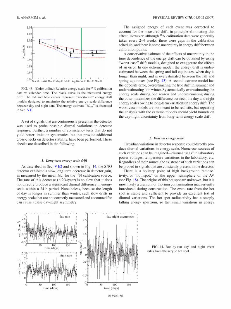
B. AHARMIM et al. PHYSICAL REVIEW C 75, 045502 (2007)
Nov 99 Jan 00 Mar 00 May 00 Jul 00 Aug 00 Oct 00 Dec 00 Mar 01
/36.0
6w
inN
0.96
0.97
0.98
0.99
1
1.01
1.02
1.03
1.04
FIG. 43. (Color online) Relative energy scale for 16N calibrationdata vs calendar time. The black curve is the measured energydrift. The red and blue curves represent “worst-case” energy driftmodels designed to maximize the relative energy scale differencebetween day and night data. The energy estimate “Nwin” is discussedin Sec. V E.
A set of signals that are continuously present in the detectorwas used to probe possible diurnal variations in detectorresponse. Further, a number of consistency tests that do notyield better limits on systematics, but that provide additionalcross-checks on detector stability, have been performed. Thesechecks are described in the following.
1. Long-term energy scale drift
As described in Sec. V E2 and shown in Fig. 14, the SNOdetector exhibited a slow long-term decrease in detector gain,as measured by the mean Nhit for the 16N calibration source.The rate of this decrease (∼2%/year) is so slow that it doesnot directly produce a significant diurnal difference in energyscale within a 24-h period. Nonetheless, because the lengthof day is longer in summer than winter, such slow drifts inenergy scale that are not correctly measured and accounted forcan cause a false day-night asymmetry.
The assigned energy of each event was corrected toaccount for the measured drift, in principle eliminating thiseffect. However, although 16N calibration data were generallytaken every 2–4 weeks, there were gaps in the calibrationschedule, and there is some uncertainty in energy drift betweencalibration points.
A conservative estimate of the effects of uncertainty in thetime dependence of the energy drift can be obtained by using“worst-case” drift models, designed to exaggerate the effectsof an error. In one extreme model, the energy drift is under-estimated between the spring and fall equinoxes, when day islonger than night, and is overestimated between the fall andspring equinoxes (see Fig. 43). A second extreme model hasthe opposite error, overestimating the true drift in summer andunderestimating it in winter. Systematically overestimating theenergy scale during one season and underestimating duringthe other maximizes the difference between the day and nightenergy scales owing to long-term variations in energy drift. Theworst-case models are not meant to be realistic, but repeatingthe analysis with the extreme models should yield bounds onthe day-night uncertainty from long-term energy scale drift.
2. Diurnal energy scale
Circadian variations in detector response could directly pro-duce diurnal variations in energy scale. Numerous sources ofsuch variations can be imagined—diurnal “sags” in laboratorypower voltages, temperature variations in the laboratory, etc.Regardless of their source, the existence of such variations canbe probed in signals that are constantly present in the detector.
There is a solitary point of high background radioac-tivity, or “hot spot,” on the upper hemisphere of the AV(see Fig. 18). The origins of this hot spot are unknown, but it ismost likely a uranium or thorium contamination inadvertentlyintroduced during construction. The event rate from the hotspot is stable and sufficient to provide an excellent test ofdiurnal variations. The hot spot radioactivity has a steeplyfalling energy spectrum, so that small variations in energy
-0.50
0.51
1.52
2.53
0 50 100 150
0
0.5
1
1.5
2
2.5
0 50 100 150
time (days)
rate
(ho
ur-1
)
day rate
time (days)
rate
(ho
ur-1
)
night rate
time (days)
rate
(ho
ur-1
)
day-night asymmetry
-2
-1.5
-1
-0.5
0
0.5
1
1.5
2
2.5
3
0 50 100 150
FIG. 44. Run-by-run day and night eventrates from the acrylic hot spot.
045502-56
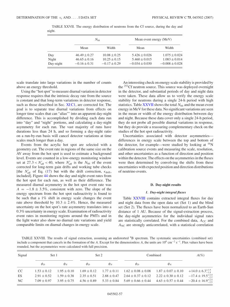
DETERMINATION OF THE νe AND . . . . I DATA SET PHYSICAL REVIEW C 75, 045502 (2007)
TABLE XXVII. The energy distribution of neutrons from the Cf source, during the day andnight.
Nhit Mean event energy (MeV)
Mean Width Mean Width
Day 46.49 ± 0.27 10.08 ± 0.25 5.426 ± 0.026 1.075 ± 0.024Night 46.65 ± 0.16 10.25 ± 0.15 5.460 ± 0.015 1.083 ± 0.014Day-night −0.16 ± 0.31 −0.17 ± 0.29 −0.034 ± 0.030 −0.008 ± 0.028
scale translate into large variations in the number of countsabove an energy threshold.
Using the “hot spot” to measure diurnal variation in detectorresponse requires that the intrinsic decay rate from the sourceis constant and that long-term variations in detector response,such as those described in Sec. XI C1, are corrected for. Thegoal is to separate true diurnal variations from effects onlonger time scales that can “alias”’ into an apparent day-nightdifference. This is accomplished by dividing each data runinto “day” and “night” portions, and calculating a day-nightasymmetry for each run. The vast majority of runs havedurations less than 24 h, and so forming a day-night ratioon a run-by-run basis will cancel detector variations at timescales much longer than a day.
Events from the acrylic hot spot are selected with ageometry cut. The event rate in regions of the same size on theAV away from the hot spot is used to estimate a backgroundlevel. Events are counted in a low-energy monitoring windowset at 27.3 < N ′
eff < 40, where N ′eff is the Nhit of the event
corrected for long-term gain drifts and working tube checks[the N ′
eff of Eq. (17) but with the drift correction, εdrift,included]. Figure 44 shows the day and night event rates fromthe hot spot for each run, as well as their difference. Themeasured diurnal asymmetry in the hot spot event rate wasA = −1.8 ± 3.5%, consistent with zero. The slope of theenergy spectrum from the hot spot radioactivity is found tobe such that a 1% shift in energy scale changes the eventrate above threshold by 10.3 ± 2.4%. Hence, the measureduncertainty on the hot spot’s rate asymmetry translates into a0.3% uncertainty in energy scale. Examination of radioactivityevent rates in monitoring regions around the PMTs and inthe light water also show no diurnal rate variations and yieldcomparable limits on diurnal changes in energy scale.
An interesting check on energy scale stability is provided bythe 252Cf neutron source. This source was deployed overnightin the detector, and substantial periods of day and night datawere taken. These data allow us to verify the energy scalestability for neutrons during a single 24-h period with highstatistics. Table XXVII shows the total Nhit and the mean eventenergy in MeV for these data. No significant variations are seenin the mean or width of the energy distribution between dayand night. Because these data cover only a single 24-h period,they do not probe all possible diurnal variations in response,but they do provide a reassuring complementary check on thestudies of the hot spot radioactivity.
Uncertainties associated with detector asymmetries—differences in energy scale between the top and bottom ofthe detector, for example—were studied by looking at 16Ncalibration source events and measuring the scale, resolution,and other uncertainties as a function of direction and positionwithin the detector. The effects on the asymmetries in the fluxeswere then determined by convolving the shifts from theseuncertainties with expected position and direction distributionsof neutrino events.
D. Day-night results
1. Day-night integral fluxes
Table XXVIII contains extracted integral fluxes for dayand night data from the open data set (Set 1) and the blindset (Set 2). The fluxes have been normalized to an Earth-Sundistance of 1 AU. Because of the signal-extraction process,the day-night asymmetries for the individual signal ratesare statistically correlated. For the combined data, ACC andANC are strongly anticorrelated, with a statistical correlation
TABLE XXVIII. The results of signal extraction, assuming an undistorted 8B spectrum. The systematic uncertainties (combined set)include a component that cancels in the formation of the A. Except for the dimensionless A, the units are 106 cm−2 s−1. Flux values have beenrounded, but the asymmetries were calculated with full precision.
Signal Set 1 Set 2 Combined A(%)
φD φN φD φN φD φN
CC 1.53 ± 0.12 1.95 ± 0.10 1.69 ± 0.12 1.77 ± 0.11 1.62 ± 0.08 ± 0.08 1.87 ± 0.07 ± 0.10 +14.0 ± 6.3+1.5−1.4
ES 2.91 ± 0.52 1.59 ± 0.38 2.35 ± 0.51 2.88 ± 0.47 2.64 ± 0.37 ± 0.12 2.22 ± 0.30 ± 0.12 −17.4 ± 19.5+2.4−2.2
NC 7.09 ± 0.97 3.95 ± 0.75 4.56 ± 0.89 5.33 ± 0.84 5.69 ± 0.66 ± 0.44 4.63 ± 0.57 ± 0.44 −20.4 ± 16.9+2.4−2.5
045502-57
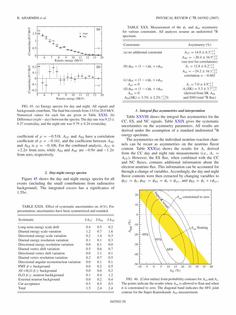
B. AHARMIM et al. PHYSICAL REVIEW C 75, 045502 (2007)
0
0.5
1
1.5
5 6 7 8 9 10 11 12 13 20
NightDay
Kinetic energy (MeV)
(Cou
nts/
day)
/0.5
MeV (a)
Kinetic energy (MeV)
(Cou
nts/
day)
/0.5
MeV (b)
-0.2
-0.1
0
0.1
0.2
5 6 7 8 9 10 11 12 13 20
FIG. 45. (a) Energy spectra for day and night. All signals andbackgrounds contribute. The final bin extends from 13.0 to 20.0 MeV.Numerical values for each bin are given in Table XXXI. (b)Difference (night−day) between the spectra. The day rate was 9.23±0.27 events/day, and the night rate was 9.79 ± 0.24 events/day.
coefficient of ρ = −0.518. ACC and AES have a correlationcoefficient of ρ = −0.161, and the coefficient between ANC
and AES is ρ = −0.106. For the combined analysis, ACC is+2.2σ from zero, while AES and ANC are −0.9σ and −1.2σ
from zero, respectively.
2. Day-night energy spectra
Figure 45 shows the day and night energy spectra for allevents (including the small contributions from radioactivebackground). The integrated excess has a significance of1.55σ .
TABLE XXIX. Effect of systematic uncertainties on A(%). Forpresentation, uncertainties have been symmetrized and rounded.
Systematic δACC δAES δANC
Long-term energy scale drift 0.4 0.5 0.2Diurnal energy scale variation 1.2 0.7 1.6Directional energy scale variation 0.2 1.4 0.3Diurnal energy resolution variation 0.1 0.1 0.3Directional energy resolution variation 0.0 0.1 0.0Diurnal vertex shift variation 0.5 0.6 0.7Directional vertex shift variation 0.0 1.1 0.1Diurnal vertex resolution variation 0.2 0.7 0.5Directional angular reconstruction variation 0.0 0.1 0.1PMT β-γ background 0.0 0.2 0.5AV+H2O β-γ background 0.0 0.6 0.2D2O β-γ , neutron backkground 0.1 0.4 1.2External neutron background 0.0 0.2 0.4Cut acceptance 0.5 0.5 0.5Total 1.5 2.4 2.4
TABLE XXX. Measurement of the φe and φtot asymmetryfor various constraints. All analyses assume an undistorted 8Bspectrum.
Constraints Asymmetry (%)
(a) no additional constraint ACC = 14.0 ± 6.3+1.5−1.4
ANC = −20.4 ± 16.9+2.4−2.5
(see text for correlations)(b) φES = (1 − ε)φe + εφtot Ae = 12.8 ± 6.2+1.5
−1.4
Atot = −24.2 ± 16.1+2.4−2.5
correlation = −0.602(c) φES = (1 − ε)φe + εφtot
Atot = 0 Ae = 7.0 ± 4.9+1.3−1.2
(d) φES = (1 − ε)φe + εφtot Ae(SK) = 5.3 ± 3.7+2.0−1.7
Atot = 0 (derived from SK AES
AES(SK) = 3.3% ± 2.2%+1.3−1.2% and SNO total 8B flux)
3. Integral flux asymmetries and interpretation
Table XXVIII shows the integral flux asymmetries for theCC, ES, and NC signals. Table XXIX gives the systematicuncertainties on the asymmetry parameters. All results arederived under the assumption of a standard undistorted 8Benergy spectrum.
The asymmetries on the individual neutrino reaction chan-nels can be recast as asymmetries on the neutrino flavorcontent. Table XXX(a) shows the results for Ae derivedfrom the CC day and night rate measurements (i.e., Ae =ACC). However, the ES flux, when combined with the CCand NC fluxes, contains additional information about theelectron neutrino flux. This information can be accounted forthrough a change of variables. Accordingly, the day and nightflavor contents were then extracted by changing variables toφCC = φe, φNC = φtot = φe + φµτ , and φES = φe + εφµτ ,
A (%)
A
(
%)
e
tot
tot constrained to zeroA
tot floatingA
68%
95%99%
Super-K result
-50
-40
-30
-20
-10
0
10
20
-10 -5 0 5 10 15 20 25 30 35 40
FIG. 46. (Color online) Joint probability contours for Atot and Ae.The points indicate the results when Atot is allowed to float and whenit is constrained to zero. The diagonal band indicates the 68% jointcontour for the Super-Kamiokande AES measurement.
045502-58
DETERMINATION OF THE νe AND . . . . I DATA SET PHYSICAL REVIEW C 75, 045502 (2007)
where ε ≡ 1/6.48 is the ratio of the average ES crosssections above Teff = 5 MeV for νµτ and νe. Table XXX(b)shows the asymmetries of φe and φtot with this additionalconstraint from the ES rate measurements. This analysisallowed for an asymmetry in the total flux of 8B neutrinos(nonzero Atot), with the measurements of Ae and Atot beingstrongly anticorrelated. Figure 46 shows the Ae versus Atot
joint probability contours. Forcing Atot = 0, as predicted byactive-only models, yielded the result in Table XXX(c) ofAe = 7.0 ± 4.9(stat.)+1.3
−1.2% (syst.)Prior to SNO, the only day-night measurements of solar
neutrinos were those from the Super-Kamiokande experiment.Because Super-Kamiokande measures the elastic scatteringrate, which is sensitive to a linear combination of electronand nonelectron neutrino rates, its measurements alone cannotseparately determine Ae and Atot. However, the SNO resultscan be used to break this covariance in the Super-Kamiokanderesults. The Super-Kamiokande (SK) Collaboration measuredAES(SK) = 3.3 ± 2.2%(stat.)+1.3
−1.2% (syst.) [5]. The ES mea-surement includes a neutral current component, which reducesthe asymmetry for this reaction relative to Ae [82]. AES(SK)may be converted to an equivalent electron flavor asymmetryby using the total neutrino flux measured by SNO, yieldingAe(SK) = 5.3 ± 3.7+2.0
−1.7 [Table XXX(d)]. This value is ingood agreement with SNO’s direct measurement of Ae, asseen in Fig. 46. Taking a weighted average of the SNO andSuper-Kamiokande measurements of Ae yields an asymmetryof Ae = 6.0 ± 3.2%.
XII. SUMMARY AND CONCLUSIONS
We have detailed here the results from the Sudbury NeutrinoObservatory’s Phase I data set. The Phase I data were takenwith an integral exposure to solar 8B neutrinos of 0.65kiloton-year. Heavy water, without any additives, was boththe target and detection medium. The heavy water providedus with three neutrino detection reactions: a charged currentreaction exclusive to the νe, a neutral current reaction sensitiveto all flavors, and an elastic scattering reaction that is primarilysensitive to νe but has a small sensitivity to other flavors. Underthe assumption that the solar 8B flux is composed entirely of νesand that its spectrum is undistorted, we find that the measuredfluxes using each of the three reactions are
φCC = 1.76+0.06−0.05 (stat.)+0.09
−0.09 (syst.) × 106 cm−2s−1,
φES = 2.39+0.24−0.23 (stat.)+0.12
−0.12 (syst.) × 106 cm−2s−1,
φNC = 5.09+0.44−0.43 (stat.)+0.46
−0.43 (syst.) × 106 cm−2s−1.
The flux of neutrinos measured by φNC is significantly largerthan that measured by φCC, thus leading to the conclusionthat neutrinos of flavors other than νe must be a substantialcomponent of the solar flux. Resolving these fluxes directlyinto flavor components yields
φ(νe) = 1.76+0.05−0.05 (stat.)+0.09
−0.09 (syst.) × 106 cm−2s−1,
φ(νµτ ) = 3.41+0.45−0.45 (stat.)+0.48
−0.45 (syst.) × 106 cm−2s−1,
showing that φ(νµτ ) is 5.3σ away from zero. The total flux of8B neutrinos, as measured by φNC, is in excellent agreementwith the predictions of standard solar models.
We have also looked for an asymmetry in the day andnight neutrino fluxes, as would be expected for neutrinooscillations driven by the MSW effect. We find that theday-night asymmetry in the electron neutrino flux is
Ae = 7.0 ± 4.9 (stat.)+1.3−1.2% (syst.)
when we constrain the day-night asymmetry in the total fluxto be zero.
These results collectively represent the first solar-model-independent measurements of the solar 8B neutrino flux andthe first inclusive appearance measurement of neutrino oscil-lations. In addition, they provide the first direct confirmationof the predictions of the SSM and have thus solved thelong-standing solar neutrino problem.
ACKNOWLEDGMENTS
This research was supported in Canada by Natural Sci-ences and Engineering Research Council, Industry Canada,National Research Council, Northern Ontario Heritage Fund,Atomic Energy of Canada, Ltd., Ontario Power Genera-tion, High Performance Computing Virtual Laboratory, andCanada Foundation for Innovation; in the United States byDepartment of Energy, National Energy Research ScientificComputing Center, and Alfred P. Sloan Foundation; and in theUnited Kingdom by Particle Physics and Astronomy ResearchCouncil. We thank the SNO technical staff for their strongcontributions. We thank Inco, Ltd., for hosting this project.
APPENDIX A: APPROACH TO ESTIMATION OF MIXINGPARAMETERS FOR TWO-NEUTRINO OSCILLATIONS
In Sec. X, the measurements of the rates of the three eventtypes—CC, NC, and ES—were made under the assumptionthat the 8B energy spectrum is undistorted. These measure-ments thus provide a null hypothesis test that neutrinos fromthe Sun change flavor on their way to detectors on Earth. Asshown in Sec. X, this null hypothesis was rejected at 5.3σ . Toderive constraints on mixing parameters, however, we mustexplicitly take into account the oscillation model, which mayalter the shape of the neutrino spectra.
In our Phase I Day-Night paper [18], we reported our firstconstraints on the mixing parameters including data from SNOand other solar neutrino experiments. For that analysis, westart from the day and night energy spectra reported here inSec. XI, rather than using the null hypothesis results ofSec. X or the asymmetry reported in Sec. XI. In this section,we describe the methods used in the Day-Night paper [18] toextract these bounds.
A. Outline of method
To generate MSW contours using the data presented in thisarticle, we use a “forward fitting” technique [83]. We make
045502-59
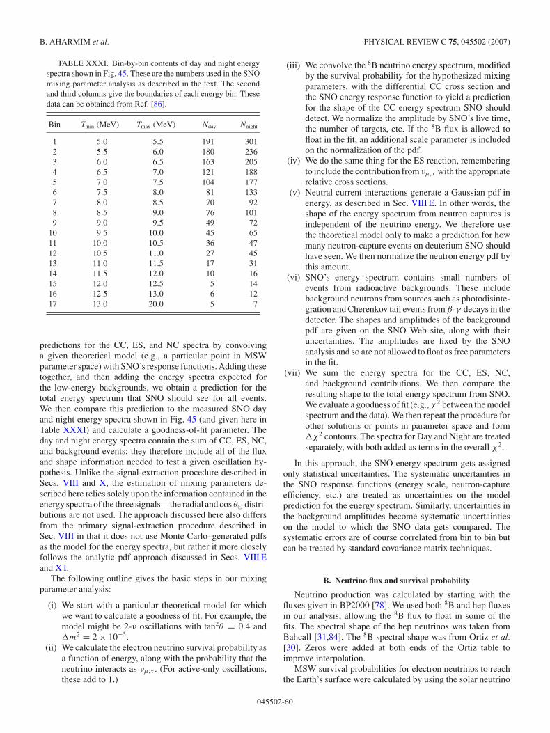
B. AHARMIM et al. PHYSICAL REVIEW C 75, 045502 (2007)
TABLE XXXI. Bin-by-bin contents of day and night energyspectra shown in Fig. 45. These are the numbers used in the SNOmixing parameter analysis as described in the text. The secondand third columns give the boundaries of each energy bin. Thesedata can be obtained from Ref. [86].
Bin Tmin (MeV) Tmax (MeV) Nday Nnight
1 5.0 5.5 191 3012 5.5 6.0 180 2363 6.0 6.5 163 2054 6.5 7.0 121 1885 7.0 7.5 104 1776 7.5 8.0 81 1337 8.0 8.5 70 928 8.5 9.0 76 1019 9.0 9.5 49 72
10 9.5 10.0 45 6511 10.0 10.5 36 4712 10.5 11.0 27 4513 11.0 11.5 17 3114 11.5 12.0 10 1615 12.0 12.5 5 1416 12.5 13.0 6 1217 13.0 20.0 5 7
predictions for the CC, ES, and NC spectra by convolvinga given theoretical model (e.g., a particular point in MSWparameter space) with SNO’s response functions. Adding thesetogether, and then adding the energy spectra expected forthe low-energy backgrounds, we obtain a prediction for thetotal energy spectrum that SNO should see for all events.We then compare this prediction to the measured SNO dayand night energy spectra shown in Fig. 45 (and given here inTable XXXI) and calculate a goodness-of-fit parameter. Theday and night energy spectra contain the sum of CC, ES, NC,and background events; they therefore include all of the fluxand shape information needed to test a given oscillation hy-pothesis. Unlike the signal-extraction procedure described inSecs. VIII and X, the estimation of mixing parameters de-scribed here relies solely upon the information contained in theenergy spectra of the three signals—the radial and cos θ� distri-butions are not used. The approach discussed here also differsfrom the primary signal-extraction procedure described inSec. VIII in that it does not use Monte Carlo–generated pdfsas the model for the energy spectra, but rather it more closelyfollows the analytic pdf approach discussed in Secs. VIII Eand X I.
The following outline gives the basic steps in our mixingparameter analysis:
(i) We start with a particular theoretical model for whichwe want to calculate a goodness of fit. For example, themodel might be 2-ν oscillations with tan2θ = 0.4 and�m2 = 2 × 10⁻⁵.
(ii) We calculate the electron neutrino survival probability asa function of energy, along with the probability that theneutrino interacts as νµ,τ . (For active-only oscillations,these add to 1.)
(iii) We convolve the 8B neutrino energy spectrum, modifiedby the survival probability for the hypothesized mixingparameters, with the differential CC cross section andthe SNO energy response function to yield a predictionfor the shape of the CC energy spectrum SNO shoulddetect. We normalize the amplitude by SNO’s live time,the number of targets, etc. If the 8B flux is allowed tofloat in the fit, an additional scale parameter is includedon the normalization of the pdf.
(iv) We do the same thing for the ES reaction, rememberingto include the contribution from νµ,τ with the appropriaterelative cross sections.
(v) Neutral current interactions generate a Gaussian pdf inenergy, as described in Sec. VIII E. In other words, theshape of the energy spectrum from neutron captures isindependent of the neutrino energy. We therefore usethe theoretical model only to make a prediction for howmany neutron-capture events on deuterium SNO shouldhave seen. We then normalize the neutron energy pdf bythis amount.
(vi) SNO’s energy spectrum contains small numbers ofevents from radioactive backgrounds. These includebackground neutrons from sources such as photodisinte-gration and Cherenkov tail events from β-γ decays in thedetector. The shapes and amplitudes of the backgroundpdf are given on the SNO Web site, along with theiruncertainties. The amplitudes are fixed by the SNOanalysis and so are not allowed to float as free parametersin the fit.
(vii) We sum the energy spectra for the CC, ES, NC,and background contributions. We then compare theresulting shape to the total energy spectrum from SNO.We evaluate a goodness of fit (e.g., χ2 between the modelspectrum and the data). We then repeat the procedure forother solutions or points in parameter space and form�χ2 contours. The spectra for Day and Night are treatedseparately, with both added as terms in the overall χ2.
In this approach, the SNO energy spectrum gets assignedonly statistical uncertainties. The systematic uncertainties inthe SNO response functions (energy scale, neutron-captureefficiency, etc.) are treated as uncertainties on the modelprediction for the energy spectrum. Similarly, uncertainties inthe background amplitudes become systematic uncertaintieson the model to which the SNO data gets compared. Thesystematic errors are of course correlated from bin to bin butcan be treated by standard covariance matrix techniques.
B. Neutrino flux and survival probability
Neutrino production was calculated by starting with thefluxes given in BP2000 [78]. We used both 8B and hep fluxesin our analysis, allowing the 8B flux to float in some of thefits. The spectral shape of the hep neutrinos was taken fromBahcall [31,84]. The 8B spectral shape was from Ortiz et al.[30]. Zeros were added at both ends of the Ortiz table toimprove interpolation.
MSW survival probabilities for electron neutrinos to reachthe Earth’s surface were calculated by using the solar neutrino
045502-60
DETERMINATION OF THE νe AND . . . . I DATA SET PHYSICAL REVIEW C 75, 045502 (2007)
production regions and electron density profile given inBP2000 [78]. Calculations of vacuum oscillation survivalprobabilities were not averaged over the production regionsin the Sun but were averaged over the annual variation of theEarth-Sun distance. Survival probabilities for the quasivacuumoscillation region between the vacuum and MSW regimeswere calculated with the analytic procedure of Lisi et al. [85].Survival probabilities for electron neutrinos traveling throughthe Earth were calculated by using the electron density profiletaken from Ref. [87].
A number of comparisons and checks were carried out toensure our prescription was consistent with others found in theliterature. For example, our calculations suggest Earth regen-eration effects should be strong in SNO for 10-MeV neutrinoswhen δm2 ≈ 10−5 eV2, similar to the result found in Ref. [80],and, as also found in Ref. [88], we find that no significant Earthregeneration occurs for δm2/E < 10−8 eV2/MeV.
C. Interaction cross sections
For interactions in SNO, neutrino-deuteron CC and NCinteraction cross sections were taken from the effective fieldtheory calculations of Butler et al. [32]. A value of 5.6fm3
was adopted for the L1A counter term in these calculations toprovide good agreement with the potential model calculationsof Nakamura et al. [33]. Neutrino-electron elastic scatteringcross sections were calculated by using the formulas given inBahcall [31]. In addition, neutrino cross sections on chlorineand gallium needed for global fits were those of Bahcall [84]. Apoint was added to the table for chlorine at 0.861 MeV (2.67×10−42 cm2, taken from Bahcall [31]), to help get the correctcontribution from 7Be neutrinos to the chlorine experiment.
D. Calculation of CC and ES electron spectra
The prediction for the measured energy spectra for the recoilelectrons from the CC reaction is given by Eq. (43), integratedover the detector live time and multiplied by the number oftargets, ND:
dNCC
dTeff= ND
∫live time
dt
∫ ∞
0dEν
d�e
dEν
×∫ ∞
0dTe
dσCC(Eν)
dTe
R(Te, Teff), (A1)
where d�e/dEν is the differential flux (the energy spectrum)of electron neutrinos at the detector calculated as describedin Sec. A2 (and includes the survival probability for thehypothesized mixing parameters), dσCC/dTe is the CC ν − d
differential cross section with respect to the true recoilelectron kinetic energy Te (discussed in Sec. A3 and furtherin Secs. IV A and X), and R(Te, T ) is the detector responsefunction to electrons given in Eq. (42) and Table X ofSec. VIII E. The number of deuteron targets, ND , is given inSec. IX D1 for 1000 tonnes of SNO heavy water and must bemultiplied by the fraction of the volume within SNO’s 550-cmradial cut. To calculate electron recoil spectra for comparisonof the day and night energy spectra, we integrate dNCC/dTeff
over limits corresponding to the boundaries of eachspectral bin.
Except for a contribution from nonelectron neutrinos, theprediction for the measured electron spectrum for the ESreaction is similar:
dNES
dTeff= ne
∫live time
dt
∫ ∞
0dEν
[d�e
dEν
×∫ ∞
0dTe
dσ eES(Eν)
dTe
R(Te, Teff) + d�µ,τ
dEν
×∫ ∞
0dTe
dσµ,τ
ES (Eν)
dTe
(Eν)R(Te, Teff),
](A2)
where d�µ,τ /dEν is the energy spectrum of muon and tauneutrinos at the detector, and ne is the total number of targetelectrons. Assuming only active neutrinos, we have
d�SSM
dEν
= d�e
dEν
+ d�µ,τ
Eν
. (A3)
It, too, must be scaled by the fraction of the volume inside550 cm. Like the differential CC rate, we integrate dNES/dTeff
to provide estimates of the number of events in each recoil-electron energy bin.
E. Calculation of detected NC neutron rate
As described in Sec. VIII E, the “spectrum” of eventsfrom the NC reaction is just the response of the detector tothe monoenergetic γ rays, and we have used a Gaussian tocharacterize the shape of this effective kinetic energy spectrumwith a mean of Tγ = 5.08 MeV and a width of σγ = 1.11 MeV.We therefore only need to calculate the absolute normalizationof this distribution, which depends in part on the number ofneutrons produced, N
prodNC , through the NC reaction:
NprodNC = ND
∫live time
dt
∫ ∞
0dEν
d�SSM
dEν
σNC(Eν), (A4)
where σNC(Eν) is the total NC cross section as a function ofneutrino energy.
To convert the number of neutrons produced by the NCreaction, Nprod
NC , to the number actually detected, NdetNC, we need
to multiply by the neutron-capture and detection efficiencies.As detailed in Sec. IX E, the probability that a neutrongenerated at a random location inside the 600-cm-radius AVwill capture on a deuteron is 29.9 ± 1.1%. Not all of thecaptured neutrons will be inside SNO’s fiducial volume andabove SNO’s energy threshold. As also described in Sec. IX E,for neutrons generated throughout the AV, 14.4 ± 0.53% willbe detected inside 550 cm and above T = 5 MeV. We thereforehave
NdetNC = 0.144 × N
prodNC .
Note that this differs from the calculation for the CC and ESevents, for which we multiplied the total number producedin each effective kinetic energy bin by just the ratio of the550-cm-radius fiducial volume to the total 600-cm-radius AVvolume.
045502-61
B. AHARMIM et al. PHYSICAL REVIEW C 75, 045502 (2007)
For the purposes of constructing predicted energy spectrafor comparison to our measured day and night spectra, webreak the total detection probability of 14.4% into an energycomponent and a radial component, to allow easier applicationof systematic errors on energy scale and radial reconstruction.With this separation, we find that
27.01±0.99% of NC neutrons capture on deuterons inside550 cm, producing events with detectable Cherenkovlight, and
53.2% of all neutrons have reconstructed effective kineticenergies above Teff > 5 MeV, as can be determined byusing the energy spectrum for 6.25-MeV γ rays givenhere and in Sec. VIII E.
We can now recalculate a new neutron detection efficiencyfor varying shifts in (for example) energy scale by reevaluatingwhat fraction of the neutron energy spectrum is above thethreshold, then multiplying by the “radial” part, 27.01%.
F. Live time
As discussed in Sec. IX and summarized in Table XII,the “day” live time for the SNO Phase I data set measured128.5 days and the “night” live time 177.9 days. Figure 35showed the distribution of this live time over 480 bins in thezenith angle cos θZ . The values in the figure are given here inTables XXXII and XXXIII.
G. Corrections to the SNO calculations
The number of events calculated needs to be corrected forthe signal loss incurred by the application of the cuts describedin Sec. V. The loss for each signal and the uncertainties on theselosses are listed in Sec. IX C4. The same losses apply to boththe day and night spectrum and are treated as uncorrelated.
H. Backgrounds
As discussed in Sec. VII, there are two primary sourcesof backgrounds to the neutrino signals: 1. neutrons fromphotodisintegration and other processes and 2. low-energyβ-γ (‘Cherenkov’) backgrounds from radioactivity inside andoutside the fiducial volume. The two sources of background areessentially independent of one another. The overall summaryof the backgrounds and uncertainties are listed in Table IX.In the fits for the mixing parameters, the asymmetric errorbars for the low-energy backgrounds were symmetrized bytaking their average. The background event numbers givenin Table IX represent the total number of detected events,and they therefore do not need any further correction forthe cut losses described in the previous section, live time,energy threshold, or fiducial volume. Table XXXIV shows thebin-by-bin background event numbers divided between dayand night, with their uncertainties. These are the numbers usedin the calculation of the mixing parameters discussed here.
I. Incorporation of systematic uncertainties
In addition to the statistical uncertainties for each bin inthe SNO spectra, there are systematic uncertainties on thedetector response functions. In our forward fitting technique,these result in systematic uncertainties on the model predictionfor the total energy spectrum.
As was presented in Sec. X E, we have here also un-certainties on the amplitudes of the backgrounds, on theoverall normalization of the signals, and on the model weuse to create our predictions for the signal energy spectra.Unlike the primary method described in Sec. X E, here weincorporate the uncertainties on the model not by shiftingand “smearing” Monte Carlo–generated pdfs but by directlyvarying the parameters in the analytic response functions. Forexample, we characterized the energy response to electronswith the Gaussian shown in Eq. (42),
R(Teff, Te) = 1√(2π )σT (Te)
exp
[− (Teff − Te − �T )2
2σ 2T (Te)
],
in which both the energy resolution σT and the energyscale offset �T are parameters for which we have measuredsystematic uncertainties. To propagate these uncertainties, wevary these parameters by the ±1σ uncertainties and recalculatethe predicted energy spectra through the convolution ofEq. (A1). Of course, a change in the shape of the energyspectrum also leads to a change in the number of events abovethreshold for each signal, and this number is also recalculatedwhen varying the response parameters. Table X of Sec. VIIIlists all the parameter uncertainties used in creating analyticpdfs. (Because the estimation of mixing parameters we do heredoes not use solar direction information, the uncertainties onthe angular resolution listed in the table are not needed.)
Uncertainties that affect only the overall normalization—the cut acceptances, neutron-capture efficiency, target volume,etc.—are given in Sec. IX. The neutron-capture efficiency istreated as discussed in Sec. A5.
The uncertainties on the amplitudes of the backgroundsare given in Sec. VII. As explained in Sec. X E, no ad-ditional shape-related uncertainties were propagated for thebackgrounds—their pdf shapes were taken as those given inSec. VII and only the amplitudes were allowed to vary within±1σ . The uncertainties on these amplitudes were symmetrizedas described in this Appendix.
The systematic uncertainties will generally affect all bins ofthe energy spectrum in a correlated way. We therefore constructN ×N covariance matrices for the systematics, which are thenadded to the statistical uncertainties on the spectral data (adiagonal matrix) to get a total uncertainty matrix that is usedto form the SNO χ2.
J. Inclusion of other data sets
In our Phase I Day-Night paper [18], we published MSWexclusion plots using only the SNO day and night spectralinformation, as well as in combination with the results ofother solar neutrino experiments. Those analyses were based
045502-62
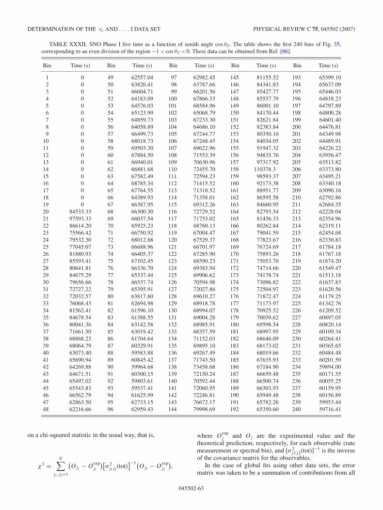
DETERMINATION OF THE νe AND . . . . I DATA SET PHYSICAL REVIEW C 75, 045502 (2007)
TABLE XXXII. SNO Phase I live time as a function of zenith angle cos θZ . The table shows the first 240 bins of Fig. 35,corresponding to an even division of the region −1 < cos θZ < 0. These data can be obtained from Ref. [86].
Bin Time (s) Bin Time (s) Bin Time (s) Bin Time (s) Bin Time (s)
1 0 49 62557.04 97 62982.45 145 81155.52 193 65399.102 0 50 63826.41 98 63787.66 146 84341.83 194 65637.093 0 51 66604.71 99 66201.56 147 85427.77 195 65446.034 0 52 64183.09 100 67866.33 148 85537.79 196 64818.235 0 53 64576.03 101 68584.96 149 86001.10 197 64797.896 0 54 65123.99 102 65068.79 150 84170.44 198 64800.287 0 55 64859.73 103 67233.30 151 82621.84 199 64601.408 0 56 64058.89 104 64686.10 152 82383.84 200 64476.819 0 57 66499.73 105 67244.77 153 80350.16 201 64349.98
10 0 58 68018.73 106 67248.45 154 84034.05 202 64489.9111 0 59 69503.30 107 69622.96 155 91947.32 203 64226.2212 0 60 67884.50 108 71553.39 156 94835.76 204 63956.4713 0 61 66940.01 109 70630.96 157 97317.92 205 63513.8214 0 62 66881.68 110 72455.70 158 110378.3 206 63373.8015 0 63 67582.49 111 72594.23 159 98593.37 207 63495.2116 0 64 68785.34 112 71415.52 160 92173.38 208 63340.1817 0 65 67764.55 113 71318.52 161 88951.77 209 63090.1618 0 66 64389.93 114 71358.01 162 86595.58 210 62792.8619 0 67 66387.95 115 69312.26 163 84660.95 211 62684.3520 84533.33 68 66300.30 116 72729.52 164 82793.54 212 62228.0421 97593.33 69 66037.54 117 71753.02 165 81456.33 213 62354.9622 86614.20 70 65925.23 118 68760.13 166 80262.84 214 62319.1123 75566.42 71 66750.92 119 67004.47 167 79041.59 215 62454.6824 79532.30 72 68012.68 120 67529.37 168 77823.67 216 62330.8325 77045.07 73 66688.96 121 66701.97 169 76724.69 217 61784.1826 81880.93 74 66405.37 122 67285.90 170 75893.26 218 61767.1827 85593.41 75 67102.45 123 68590.23 171 75053.70 219 61874.2028 80641.81 76 66336.70 124 69383.94 172 74714.66 220 61549.4729 84675.29 77 65337.44 125 69906.62 173 74178.74 221 61513.1830 79656.66 78 66537.74 126 70594.98 174 73096.82 222 61637.8331 72727.22 79 65395.91 127 72027.86 175 72504.97 223 61620.5632 72032.57 80 63817.60 128 69610.27 176 71872.47 224 61179.2533 76068.43 81 62694.98 129 68918.78 177 71173.97 225 61342.7634 81562.41 82 61596.10 130 68994.07 178 70925.52 226 61209.5235 84678.54 83 61388.55 131 69004.28 179 70039.62 227 60897.0536 80041.36 84 63142.58 132 68985.91 180 69598.54 228 60820.1437 71661.50 85 63019.42 133 68357.59 181 68997.95 229 60109.3438 68868.23 86 61704.64 134 71152.03 182 68646.09 230 60264.4139 68064.79 87 60329.91 135 69895.10 183 68173.02 231 60365.6540 63073.40 88 59583.88 136 69267.49 184 68019.66 232 60484.4841 65690.94 89 60845.42 137 71743.50 185 67635.93 233 60201.5942 64269.88 90 59964.68 138 73458.68 186 67184.90 234 59894.0043 64671.51 91 60300.15 139 72150.24 187 66659.48 235 60171.5544 65497.02 92 59803.61 140 70592.44 188 66500.74 236 60055.2545 65543.83 93 59537.41 141 72060.95 189 66303.93 237 60159.9546 66562.79 94 61625.99 142 72246.81 190 65949.48 238 60156.8947 62863.50 95 62733.15 143 76672.17 191 65782.26 239 59953.4448 62216.66 96 62959.43 144 79998.69 192 65350.60 240 59716.41
on a chi-squared statistic in the usual way, that is,
χ2 =N∑
j1,j2=1
(Oj1 − O
expj1
)[σ 2
j1j2(tot)
]−1(Oj2 − O
expj2
),
where Oexpj and Oj are the experimental value and the
theoretical prediction, respectively, for each observable (ratemeasurement or spectral bin), and [σ 2
j1j2(tot)]−1 is the inverseof the covariance matrix for the observables.
In the case of global fits using other data sets, the errormatrix was taken to be a summation of contributions from all
045502-63
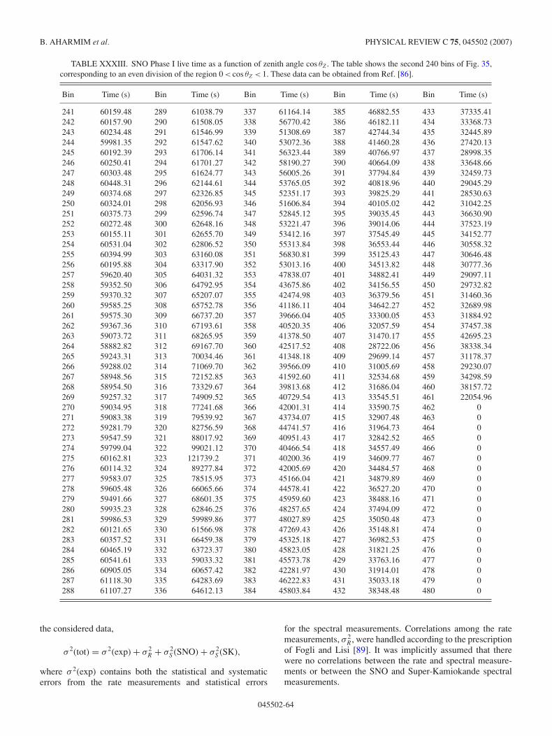
B. AHARMIM et al. PHYSICAL REVIEW C 75, 045502 (2007)
TABLE XXXIII. SNO Phase I live time as a function of zenith angle cos θZ . The table shows the second 240 bins of Fig. 35,corresponding to an even division of the region 0 < cos θZ < 1. These data can be obtained from Ref. [86].
Bin Time (s) Bin Time (s) Bin Time (s) Bin Time (s) Bin Time (s)
241 60159.48 289 61038.79 337 61164.14 385 46882.55 433 37335.41242 60157.90 290 61508.05 338 56770.42 386 46182.11 434 33368.73243 60234.48 291 61546.99 339 51308.69 387 42744.34 435 32445.89244 59981.35 292 61547.62 340 53072.36 388 41460.28 436 27420.13245 60192.39 293 61706.14 341 56323.44 389 40766.97 437 28998.35246 60250.41 294 61701.27 342 58190.27 390 40664.09 438 33648.66247 60303.48 295 61624.77 343 56005.26 391 37794.84 439 32459.73248 60448.31 296 62144.61 344 53765.05 392 40818.96 440 29045.29249 60374.68 297 62326.85 345 52351.17 393 39825.29 441 28530.63250 60324.01 298 62056.93 346 51606.84 394 40105.02 442 31042.25251 60375.73 299 62596.74 347 52845.12 395 39035.45 443 36630.90252 60272.48 300 62648.16 348 53221.47 396 39014.06 444 37523.19253 60155.11 301 62655.70 349 53412.16 397 37545.49 445 34152.77254 60531.04 302 62806.52 350 55313.84 398 36553.44 446 30558.32255 60394.99 303 63160.08 351 56830.81 399 35125.43 447 30646.48256 60195.88 304 63317.90 352 53013.16 400 34513.82 448 30777.36257 59620.40 305 64031.32 353 47838.07 401 34882.41 449 29097.11258 59352.50 306 64792.95 354 43675.86 402 34156.55 450 29732.82259 59370.32 307 65207.07 355 42474.98 403 36379.56 451 31460.36260 59585.25 308 65752.78 356 41186.11 404 34642.27 452 32689.98261 59575.30 309 66737.20 357 39666.04 405 33300.05 453 31884.92262 59367.36 310 67193.61 358 40520.35 406 32057.59 454 37457.38263 59073.72 311 68265.95 359 41378.50 407 31470.17 455 42695.23264 58882.82 312 69167.70 360 42517.52 408 28722.06 456 38338.34265 59243.31 313 70034.46 361 41348.18 409 29699.14 457 31178.37266 59288.02 314 71069.70 362 39566.09 410 31005.69 458 29230.07267 58948.56 315 72152.85 363 41592.60 411 32534.68 459 34298.59268 58954.50 316 73329.67 364 39813.68 412 31686.04 460 38157.72269 59257.32 317 74909.52 365 40729.54 413 33545.51 461 22054.96270 59034.95 318 77241.68 366 42001.31 414 33590.75 462 0271 59083.38 319 79539.92 367 43734.07 415 32907.48 463 0272 59281.79 320 82756.59 368 44741.57 416 31964.73 464 0273 59547.59 321 88017.92 369 40951.43 417 32842.52 465 0274 59799.04 322 99021.12 370 40466.54 418 34557.49 466 0275 60162.81 323 121739.2 371 40200.36 419 34609.77 467 0276 60114.32 324 89277.84 372 42005.69 420 34484.57 468 0277 59583.07 325 78515.95 373 45166.04 421 34879.89 469 0278 59605.48 326 66065.66 374 44578.41 422 36527.20 470 0279 59491.66 327 68601.35 375 45959.60 423 38488.16 471 0280 59935.23 328 62846.25 376 48257.65 424 37494.09 472 0281 59986.53 329 59989.86 377 48027.89 425 35050.48 473 0282 60121.65 330 61566.98 378 47269.43 426 35148.81 474 0283 60357.52 331 66459.38 379 45325.18 427 36982.53 475 0284 60465.19 332 63723.37 380 45823.05 428 31821.25 476 0285 60541.61 333 59033.32 381 45573.78 429 33763.16 477 0286 60905.05 334 60657.42 382 42281.97 430 31914.01 478 0287 61118.30 335 64283.69 383 46222.83 431 35033.18 479 0288 61107.27 336 64612.13 384 45803.84 432 38348.48 480 0
the considered data,
σ 2(tot) = σ 2(exp) + σ 2R + σ 2
S (SNO) + σ 2S (SK),
where σ 2(exp) contains both the statistical and systematicerrors from the rate measurements and statistical errors
for the spectral measurements. Correlations among the ratemeasurements, σ 2
R , were handled according to the prescriptionof Fogli and Lisi [89]. It was implicitly assumed that therewere no correlations between the rate and spectral measure-ments or between the SNO and Super-Kamiokande spectralmeasurements.
045502-64
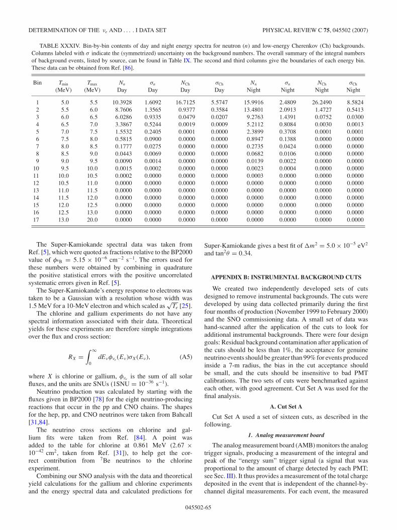
DETERMINATION OF THE νe AND . . . . I DATA SET PHYSICAL REVIEW C 75, 045502 (2007)
TABLE XXXIV. Bin-by-bin contents of day and night energy spectra for neutron (n) and low-energy Cherenkov (Ch) backgrounds.Columns labeled with σ indicate the (symmetrized) uncertainty on the background numbers. The overall summary of the integral numbersof background events, listed by source, can be found in Table IX. The second and third columns give the boundaries of each energy bin.These data can be obtained from Ref. [86].
Bin Tmin Tmax Nn σn NCh σCh Nn σn NCh σCh
(MeV) (MeV) Day Day Day Day Night Night Night Night
1 5.0 5.5 10.3928 1.6092 16.7125 5.5747 15.9916 2.4809 26.2490 8.58242 5.5 6.0 8.7606 1.3565 0.9377 0.3584 13.4801 2.0913 1.4727 0.54133 6.0 6.5 6.0286 0.9335 0.0479 0.0207 9.2763 1.4391 0.0752 0.03004 6.5 7.0 3.3867 0.5244 0.0019 0.0009 5.2112 0.8084 0.0030 0.00135 7.0 7.5 1.5532 0.2405 0.0001 0.0000 2.3899 0.3708 0.0001 0.00016 7.5 8.0 0.5815 0.0900 0.0000 0.0000 0.8947 0.1388 0.0000 0.00007 8.0 8.5 0.1777 0.0275 0.0000 0.0000 0.2735 0.0424 0.0000 0.00008 8.5 9.0 0.0443 0.0069 0.0000 0.0000 0.0682 0.0106 0.0000 0.00009 9.0 9.5 0.0090 0.0014 0.0000 0.0000 0.0139 0.0022 0.0000 0.0000
10 9.5 10.0 0.0015 0.0002 0.0000 0.0000 0.0023 0.0004 0.0000 0.000011 10.0 10.5 0.0002 0.0000 0.0000 0.0000 0.0003 0.0000 0.0000 0.000012 10.5 11.0 0.0000 0.0000 0.0000 0.0000 0.0000 0.0000 0.0000 0.000013 11.0 11.5 0.0000 0.0000 0.0000 0.0000 0.0000 0.0000 0.0000 0.000014 11.5 12.0 0.0000 0.0000 0.0000 0.0000 0.0000 0.0000 0.0000 0.000015 12.0 12.5 0.0000 0.0000 0.0000 0.0000 0.0000 0.0000 0.0000 0.000016 12.5 13.0 0.0000 0.0000 0.0000 0.0000 0.0000 0.0000 0.0000 0.000017 13.0 20.0 0.0000 0.0000 0.0000 0.0000 0.0000 0.0000 0.0000 0.0000
The Super-Kamiokande spectral data was taken fromRef. [5], which were quoted as fractions relative to the BP2000value of φ8B = 5.15 × 10⁻⁶ cm−2 s−1. The errors used forthese numbers were obtained by combining in quadraturethe positive statistical errors with the positive uncorrelatedsystematic errors given in Ref. [5].
The Super-Kamiokande’s energy response to electrons wastaken to be a Gaussian with a resolution whose width was1.5 MeV for a 10-MeV electron and which scaled as
√Te [25].
The chlorine and gallium experiments do not have anyspectral information associated with their data. Theoreticalyields for these experiments are therefore simple integrationsover the flux and cross section:
RX =∫ ∞
0dEνφνe
(Eν)σX(Eν), (A5)
where X is chlorine or gallium, φνeis the sum of all solar
fluxes, and the units are SNUs (1SNU = 10−36 s−1).Neutrino production was calculated by starting with the
fluxes given in BP2000 [78] for the eight neutrino-producingreactions that occur in the pp and CNO chains. The shapesfor the hep, pp, and CNO neutrinos were taken from Bahcall[31,84].
The neutrino cross sections on chlorine and gal-lium fits were taken from Ref. [84]. A point wasadded to the table for chlorine at 0.861 MeV (2.67 ×10−42 cm2, taken from Ref. [31]), to help get the cor-rect contribution from 7Be neutrinos to the chlorineexperiment.
Combining our SNO analysis with the data and theoreticalyield calculations for the gallium and chlorine experimentsand the energy spectral data and calculated predictions for
Super-Kamiokande gives a best fit of �m2 = 5.0 × 10⁻⁵ eV2
and tan2θ = 0.34.
APPENDIX B: INSTRUMENTAL BACKGROUND CUTS
We created two independently developed sets of cutsdesigned to remove instrumental backgrounds. The cuts weredeveloped by using data collected primarily during the firstfour months of production (November 1999 to February 2000)and the SNO commissioning data. A small set of data washand-scanned after the application of the cuts to look foradditional instrumental backgrounds. There were four designgoals: Residual background contamination after application ofthe cuts should be less than 1%, the acceptance for genuineneutrino events should be greater than 99% for events producedinside a 7-m radius, the bias in the cut acceptance shouldbe small, and the cuts should be insensitive to bad PMTcalibrations. The two sets of cuts were benchmarked againsteach other, with good agreement. Cut Set A was used for thefinal analysis.
A. Cut Set A
Cut Set A used a set of sixteen cuts, as described in thefollowing.
1. Analog measurement board
The analog measurement board (AMB) monitors the analogtrigger signals, producing a measurement of the integral andpeak of the “energy sum” trigger signal (a signal that wasproportional to the amount of charge detected by each PMT;see Sec. III). It thus provides a measurement of the total chargedeposited in the event that is independent of the channel-by-channel digital measurements. For each event, the measured
045502-65
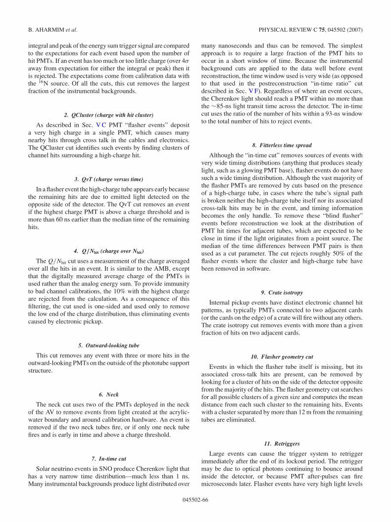
B. AHARMIM et al. PHYSICAL REVIEW C 75, 045502 (2007)
integral and peak of the energy sum trigger signal are comparedto the expectations for each event based upon the number ofhit PMTs. If an event has too much or too little charge (over 4σ
away from expectation for either the integral or peak) then itis rejected. The expectations come from calibration data withthe 16N source. Of all the cuts, this cut removes the largestfraction of the instrumental backgrounds.
2. QCluster (charge with hit cluster)
As described in Sec. V C PMT “flasher events” deposita very high charge in a single PMT, which causes manynearby hits through cross talk in the cables and electronics.The QCluster cut identifies such events by finding clusters ofchannel hits surrounding a high-charge hit.
3. QvT (charge versus time)
In a flasher event the high-charge tube appears early becausethe remaining hits are due to emitted light detected on theopposite side of the detector. The QvT cut removes an eventif the highest charge PMT is above a charge threshold and ismore than 60 ns earlier than the median time of the remaininghits.
4. Q/Nhit (charge over Nhit)
The Q/Nhit cut uses a measurement of the charge averagedover all the hits in an event. It is similar to the AMB, exceptthat the digitally measured average charge of the PMTs isused rather than the analog energy sum. To provide immunityto bad channel calibrations, the 10% with the highest chargeare rejected from the calculation. As a consequence of thisfiltering, the cut used is one-sided and used only to removethe low end of the charge distribution, thus eliminating eventscaused by electronic pickup.
5. Outward-looking tube
This cut removes any event with three or more hits in theoutward-looking PMTs on the outside of the phototube supportstructure.
6. Neck
The neck cut uses two of the PMTs deployed in the neckof the AV to remove events from light created at the acrylic-water boundary and around calibration hardware. An event isremoved if the two neck tubes fire, or if only one neck tubefires and is early in time and above a charge threshold.
7. In-time cut
Solar neutrino events in SNO produce Cherenkov light thathas a very narrow time distribution—much less than 1 ns.Many instrumental backgrounds produce light distributed over
many nanoseconds and thus can be removed. The simplestapproach is to require a large fraction of the PMT hits tooccur in a short window of time. Because the instrumentalbackground cuts are applied to the data well before eventreconstruction, the time window used is very wide (as opposedto that used in the postreconstruction “in-time ratio” cutdescribed in Sec. V F). Regardless of where an event occurs,the Cherenkov light should reach a PMT within no more thanthe ∼85-ns light transit time across the detector. The in-timecut uses the ratio of the number of hits within a 93-ns windowto the total number of hits to reject events.
8. Fitterless time spread
Although the “in-time cut” removes sources of events withvery wide timing distributions (anything that produces steadylight, such as a glowing PMT base), flasher events do not havesuch a wide timing distribution. Although the vast majority ofthe flasher PMTs are removed by cuts based on the presenceof a high-charge tube, in cases where the tube’s signal pathis broken neither the high-charge tube itself nor its associatedcross-talk hits may be in the event, and timing informationbecomes the only handle. To remove these “blind flasher”events before reconstruction we look at the distribution ofPMT hit times for adjacent tubes, which are expected to beclose in time if the light originates from a point source. Themedian of the time differences between PMT pairs is thenused as a cut parameter. The cut rejects roughly 50% of theflasher events where the cluster and high-charge tube havebeen removed in software.
9. Crate isotropy
Internal pickup events have distinct electronic channel hitpatterns, as typically PMTs connected to two adjacent cards(or the cards on the edge) of a crate will fire without any others.The crate isotropy cut removes events with more than a givenfraction of hits on two adjacent cards.
10. Flasher geometry cut
Events in which the flasher tube itself is missing, but itsassociated cross-talk hits are present, can be removed bylooking for a cluster of hits on the side of the detector oppositefrom the majority of the hits. The flasher geometry cut searchesfor all possible clusters of a given size and computes the meandistance from each such cluster to the remaining hits. Eventswith a cluster separated by more than 12 m from the remainingtubes are eliminated.
11. Retriggers
Large events can cause the trigger system to retriggerimmediately after the end of its lockout period. The retriggermay be due to optical photons continuing to bounce aroundinside the detector, or because PMT after-pulses can firemicroseconds later. Flasher events have very high light levels
045502-66
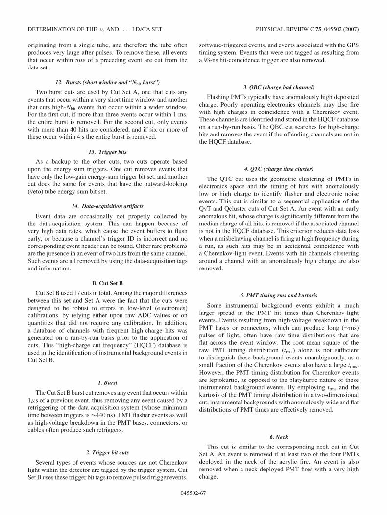
DETERMINATION OF THE νe AND . . . . I DATA SET PHYSICAL REVIEW C 75, 045502 (2007)
originating from a single tube, and therefore the tube oftenproduces very large after-pulses. To remove these, all eventsthat occur within 5µs of a preceding event are cut from thedata set.
12. Bursts (short window and “Nhit burst”)
Two burst cuts are used by Cut Set A, one that cuts anyevents that occur within a very short time window and anotherthat cuts high-Nhit events that occur within a wider window.For the first cut, if more than three events occur within 1 ms,the entire burst is removed. For the second cut, only eventswith more than 40 hits are considered, and if six or more ofthese occur within 4 s the entire burst is removed.
13. Trigger bits
As a backup to the other cuts, two cuts operate basedupon the energy sum triggers. One cut removes events thathave only the low-gain energy-sum trigger bit set, and anothercut does the same for events that have the outward-looking(veto) tube energy-sum bit set.
14. Data-acquisition artifacts
Event data are occasionally not properly collected bythe data-acquisition system. This can happen because ofvery high data rates, which cause the event buffers to flushearly, or because a channel’s trigger ID is incorrect and nocorresponding event header can be found. Other rare problemsare the presence in an event of two hits from the same channel.Such events are all removed by using the data-acquisition tagsand information.
B. Cut Set B
Cut Set B used 17 cuts in total. Among the major differencesbetween this set and Set A were the fact that the cuts weredesigned to be robust to errors in low-level (electronics)calibrations, by relying either upon raw ADC values or onquantities that did not require any calibration. In addition,a database of channels with frequent high-charge hits wasgenerated on a run-by-run basis prior to the application ofcuts. This “high-charge cut frequency” (HQCF) database isused in the identification of instrumental background events inCut Set B.
1. Burst
The Cut Set B burst cut removes any event that occurs within1µs of a previous event, thus removing any event caused by aretriggering of the data-acquisition system (whose minimumtime between triggers is ∼440 ns). PMT flasher events as wellas high-voltage breakdown in the PMT bases, connectors, orcables often produce such retriggers.
2. Trigger bit cuts
Several types of events whose sources are not Cherenkovlight within the detector are tagged by the trigger system. CutSet B uses these trigger bit tags to remove pulsed trigger events,
software-triggered events, and events associated with the GPStiming system. Events that were not tagged as resulting froma 93-ns hit-coincidence trigger are also removed.
3. QBC (charge bad channel)
Flashing PMTs typically have anomalously high depositedcharge. Poorly operating electronics channels may also firewith high charges in coincidence with a Cherenkov event.These channels are identified and stored in the HQCF databaseon a run-by-run basis. The QBC cut searches for high-chargehits and removes the event if the offending channels are not inthe HQCF database.
4. QTC (charge time cluster)
The QTC cut uses the geometric clustering of PMTs inelectronics space and the timing of hits with anomalouslylow or high charge to identify flasher and electronic noiseevents. This cut is similar to a sequential application of theQvT and Qcluster cuts of Cut Set A. An event with an earlyanomalous hit, whose charge is significantly different from themedian charge of all hits, is removed if the associated channelis not in the HQCF database. This criterion reduces data losswhen a misbehaving channel is firing at high frequency duringa run, as such hits may be in accidental coincidence witha Cherenkov-light event. Events with hit channels clusteringaround a channel with an anomalously high charge are alsoremoved.
5. PMT timing rms and kurtosis
Some instrumental background events exhibit a muchlarger spread in the PMT hit times than Cherenkov-lightevents. Events resulting from high-voltage breakdown in thePMT bases or connectors, which can produce long (∼ms)pulses of light, often have raw time distributions that areflat across the event window. The root mean square of theraw PMT timing distribution (trms) alone is not sufficientto distinguish these background events unambiguously, as asmall fraction of the Cherenkov events also have a large trms.However, the PMT timing distribution for Cherenkov eventsare leptokurtic, as opposed to the platykurtic nature of theseinstrumental background events. By employing trms and thekurtosis of the PMT timing distribution in a two-dimensionalcut, instrumental backgrounds with anomalously wide and flatdistributions of PMT times are effectively removed.
6. Neck
This cut is similar to the corresponding neck cut in CutSet A. An event is removed if at least two of the four PMTsdeployed in the neck of the acrylic fire. An event is alsoremoved when a neck-deployed PMT fires with a very highcharge.
045502-67
B. AHARMIM et al. PHYSICAL REVIEW C 75, 045502 (2007)
7. FGC (flasher geometry cut)
The FGC is the predecessor to the cut of Cut Set A with thesame name. The primary difference between them is in clusteridentification; this cut requires more PMT hits in a cluster.
8. QQP (two-charge cut)
This is a two-dimensional cut that uses the total channelcharges (from summing the charges in all hit channels) andthe integral charge from the AMB, both averaged over allPMT hits, as the cut parameters. This cut is effective againstelectrical noise, which normally has very low integral charges.Electrical discharge events, which have very high depositedcharge, would saturate the AMB integral charge channelbecause of its limited dynamic range. In such instances, thiscut identifies such discharge events by imposing additional cutcriteria on the pulse height measured by the AMB.
9. Correlated channel count rates
Electronics boards in which several adjacent channels hadhigh count rates are flagged so that events created by pickupfrom the data-acquisition readout can be removed. Electricalnoise pickup events may have a disproportional number of hitsin a single crate. Events with such concentration of hits in acrate are also removed.
10. Veto tube cut
Muons and muon-related events, as well as any event thatproduces light external to the phototube support sphere, arecut by using a combination of the veto PMTs in the neckregion of the AV, the outward-looking PMTs installed on theoutside of the phototube support sphere, and a set of 23 PMTssuspended between the phototube support sphere and the rockof the cavity.
[1] K. Eguchi et al., Phys. Rev. Lett. 90, 021802 (2003).[2] B. T. Cleveland et al., Astrophys. J. 496, 505 (1998).[3] J. N. Abdurashitov et al., Phys. Rev. C 60, 055801 (1999).[4] W. Hampel et al., Phys. Lett. B447, 127 (1999).[5] S. Fukuda et al., Phys. Rev. Lett. 86, 5651 (2001).[6] M. Altmann et al., Phys. Lett. B490, 16 (2000).[7] J. N. Bahcall, M. H. Pinsonneault, and S. Basu, Astrophys. J.
555, 990 (2001).[8] A. S. Brun, S. Turck-Chieze, and J. P. Zahn, Astrophys. J. 525,
1032 (2001).[9] N. Hata and P. Langacker, Phys. Rev. D 52, 420 (1995).
[10] K. M. Heeger and R. G. H. Robertson, Phys. Rev. Lett. 77, 3720(1996).
[11] B. Pontecorvo, Zh. Eksp. Teor. Fiz. 33, 549 (1957).[12] Z. Maki, M. Nakagawa, and S. Sakata, Prog. Theor. Phys. 28,
870 (1962).[13] L. Wolfenstein, Phys. Rev. D 17, 2369 (1978).[14] S. P. Mikheyev and A. Smirnov, Nuovo Cimento C 9, 17
(1986).[15] H. H. Chen, Phys. Rev. Lett. 55, 1534 (1985).[16] SNO Collaboration, Phys. Rev. Lett. 87, 071301 (2001).[17] SNO Collaboration, Phys. Rev. Lett. 89, 011301 (2002).[18] SNO Collaboration, Phys. Rev. Lett. 89, 011302 (2002).[19] J. Boger et al. (SNO Collaboration), Nucl. Instrum. Methods A
449, 172 (2000).[20] B. A. Moffat et al., Nucl. Instrum. Methods A 554, 255
(2005).[21] M. R. Dragowsky et al., Nucl. Instrum. Methods A 481, 284
(2002).[22] N. J. Tagg et al., Nucl. Instrum. Methods A 489, 178 (2002).[23] A. W. P. Poon et al., Nucl. Instrum. Methods A 452, 115
(2000).[24] J. F. Beacom and P. Vogel, Phys. Rev. Lett. 83, 5222 (1999).[25] G. L. Fogli, E. Lisi, A. Palazzo, and F. L. Villante, Phys. Rev. D
63, 113016 (2001).[26] F. L. Villante, G. Fiorentini, and E. Lisi, Phys. Rev. D 59, 013006
(1999).[27] M. G. Boulay, Ph.D. thesis, Queens University, 2001 (unpub-
lished).[28] M. S. Neubauer, Ph.D. thesis, University of Pennsylvania, 2001
(unpublished).
[29] K. Heeger, Ph.D. thesis, University of Washington, 2002(unpublished).
[30] C. E. Ortiz, A. Garcia, R. A. Waltz, M. Bhattacharya, and A. K.Komives, Phys. Rev. Lett. 85, 2909 (2000).
[31] J. N. Bahcall, Neutrino Astrophysics (Cambridge UniversityPress, Cambridge, 1989).
[32] M. Butler, J. W. Chen, and X. Kong, Phys. Rev. C 63, 035501(2001).
[33] S. Nakamura et al., Nucl. Phys. A707, 561 (2002).[34] A. Kurylov, M. J. Ramsey-Musolf, and P. Vogel, Phys. Rev. C
65, 055501 (2002).[35] S. Nakamura, T. Sato, V. Gudkov, and K. Kubodera, Phys. Rev.
C 63, 034617 (2001).[36] K. Kubodera and S. Nozawa, Int. J. Mod. Phys. E 3, 101
(1994).[37] W. R. Nelson, H. Hirayama, and D. W. O. Rogers, SLAC Report
No. 265, 1985 (unpublished).[38] Subsequent to the results published in Refs. [16–18], we found
that EGS4 needed a small correction to allow for the neglect ofMott terms in the electron scattering cross section and otherapproximations in the treatment of multiple scattering [90]. Theeffects of the Mott terms on the analyses presented here werefound to be negligible.
[39] M. D. Lay, Ph.D. thesis, University of Oxford, unpublished(1995).
[40] MCNP 4A, A Monte Carlo N-Particle Transport Code System,Radiation Shielding Information Center, Los Alamos NationalLaboratory, Los Alamos, Nov. 1993 (unpublished).
[41] J. C. Wang, G. L. Jensen, and J. B. Czirr, Nucl. Sci. Eng. 113,77 (1993).
[42] P. A. Aarnio et al., prepared for International Conference onMonte Carlo Simulation in High Energy and Nuclear Physics-MC 93, Tallahassee, FL, 22–26 Feb. 1993.
[43] W. Buchmuller and G. Ingelman, Hamburg, Germany: DESY(1992), p.1566.
[44] B. A. Moffat, Ph.D. thesis, Queens University, 2001 (unpub-lished).
[45] R. Ford, Ph.D. thesis, Queens University, 1999 (unpublished).[46] J. C. Zwinkels, W. F. Davidson, and C. X. Dodd, Appl. Opt. 29,
3240 (1990).[47] L. P. Boivin et al., Appl. Opt. 25, 877 (1986).
045502-68
DETERMINATION OF THE νe AND . . . . I DATA SET PHYSICAL REVIEW C 75, 045502 (2007)
[48] R. C. Smith and K. S. Baker, Appl. Opt. 20, 177 (1981).[49] T. I. Quickenden and J. A. Irvin, J. Chem. Phys. 72, 4416 (1980).[50] R. M. Pope and E. S. Fry, Appl. Opt. 36, 8710 (1997).[51] D. F. Cowen et al., IEEE Trans. Nucl. Sci. 42, 925 (1995).[52] N. K. McCauley, Ph.D. thesis, University of Oxford, 2001
(unpublished).[53] A.W. P. Poon et al., SNO Internal Memo, 2000 (unpublished).[54] M. Moorhead and X. Chen, SNO Internal Memo, SNO-STR-
00-004, 2000 (unpublished).[55] P. Wittich, Ph.D. thesis, University of Pennsylvania, 2000
(unpublished).[56] C. Jillings, Ph.D. thesis, Queens University, 2000 (unpublished).[57] A. S. Hamer, Ph.D. thesis, Queens University, 2000 (unpub-
lished).[58] P. C. Bergbusch, Ph.D. thesis, University of British Columbia,
2000 (unpublished).[59] V. L. Rusu, Ph.D. thesis, University of Pennsylvania, 2003
(unpublished).[60] T. C. Andersen et al., Nucl. Instrum. Methods A 501, 399 (2003).[61] T. C. Andersen et al., Nucl. Instrum. Methods A 501, 386 (2003).[62] I. Blevis et al., Nucl. Instrum. Methods A 517, 139 (2004).[63] R. K. Taplin, Ph.D. thesis, Oxford University, 1998 (unpub-
lished).[64] X. Chen, Ph.D. thesis, Oxford University, 1997 (unpublished).[65] G. McGregor, Ph.D. thesis, Oxford University, 2002 (unpub-
lished).[66] N. E. Holden and D. C. Hoffman, Pure Appl. Chem. 72, 1525
(2000).[67] V. Agrawal, T. K. Gaisser, P. Lipari, and T. Stanev, Phys. Rev.
D 53, 1314 (1996).[68] S. Fukuda et al., Phys. Rev. Lett. 85, 3999 (2000).[69] C. H. Llewellyn Smith, Phys. Rep. 3, 261 (1972).[70] A. Fasso, A. Ferrari, P. R. Sala, and J. Ranft, in Proceedings of
the Monte Carlo 2000 Conference, Lisbon, Portugal, 2000.[71] M. Conrad, Oxygen Isotope Compositions of Sudbury Neutrino
Observatory Heavy Water, Earth Sciences Division, LawrenceBerkeley National Laboratory, 2001 (unpublished).
[72] A. B. Balantekin and F. Loreti, AIP Conf. Proc. 243, 1143(1992).
[73] B. Aharmim et al. (SNO Collaboration), Phys. Rev. D 70,093014 (2004) [arXiv:hep-ex/0407029].
[74] J. D. Hallidy, 17O Measurement in Bruce Heavy Water Sampleswith 17O NMR, Atomic Energy of Canada Limited, 1997(unpublished).
[75] E. Kerstel, 17O Analysis of Ontario Hydro Heavy Water,Center for Isotope Research, University of Groningen, 2001(unpublished).
[76] W. C. Haxton and R. G. H. Robertson, Phys. Rev. C 59, 515(1999).
[77] F. James and M. Roos, Comput. Phys. Commun. 10, 343(1975).
[78] J. N. Bahcall, M. Pinsonneault, and S. Basu, Astrophys. J. 555,990 (2001).
[79] S. P. Mikheyev and A. Y. Smirnov, in ’86 Massive Neutrinosin Astrophysics and in Particle Physics, Proceedings of theMoriond Workshop, edited by O. Fackler and J. Tran ThanhVan (Editions Frontieres, Gif-sur-Yvette, 1986), p. 335.
[80] A. J. Baltz and J. Weneser, Phys. Rev. D 37, 3364 (1988).[81] E. Kh. Akhmedov, M. A. Tortola, and J. W. F. Valle, JHEP 05
(2004) 057.[82] J. N. Bahcall, P. I. Krastev, and A. Y. Smirnov, Phys. Rev. D 62,
093004 (2000).[83] In our more recent publications [90,91], based on data from
SNO Phase II in which NaCl was dissolved within the heavywater, we were able to use the derived fluxes and spectra fromthe signal extraction process, rather than the summed spectra asdiscussed in this article. This was possible because of the betterdiscrimination between neutrons and electrons provided by theγ cascade from neutron capture on Cl.
[84] J. N. Bahcall, http://www.sns.ias.edu/∼jnb, 2001.[85] E. Lisi, A. Marrone, D. Montanino, A. Palazzo, and S. T. Petcov,
Phys. Rev. D 63, 093002 (2001).[86] Data can be directly downloaded from http://sno.phy.
queensu.ca/sno/prlwebpage/.[87] A. M. Dziewonski and D. L. Anderson, Phys. Earth Planet. Inter.
25, 297 (1981).[88] J. N. Bahcall, P. I. Krastev, and A. Yu. Smirnov, JHEP 05 (2001)
015.[89] G. L. Fogli and E. Lisi, Astropart. Phys. 3, 185 (1995).[90] S. B. Aharmim et al., Phys. Rev. C 72, 055502 (2005).[91] S. N. Ahmed et al., Phys. Rev. Lett. 92, 181301
(2004).
045502-69