v. 2.0.3 September 2008

William Henning, lead author

i

Acknowledgements

The writing of these guidelines has involved a myriad of resources. Besides the author’s personal experience with different manufacturers’ hardware and software for classical real-time (RT) Global Navigation Satellite Systems (GNSS) positioning for over a dozen years, the internet was the primary source for definitive documents and discussions. Additionally, many agencies have published single-base guidelines of some sort over the years to aid their users in the application of the technology and to provide consistency with the results. The following are gratefully acknowledged as sources for research and information:

• National Geodetic Survey (NGS)– publications and internal documents • NGS – Corbin , VA. Laboratory and Training Center • Major GNSS hardware/software manufacturers’ sites • National Oceanic and Atmospheric Administration (NOAA) Space Weather

Prediction Center • Bureau of Land Management • U.S. Forest Service • Institute of Navigation (ION) proceedings • California Department of Transportation • Florida Department of Transportation • Michigan Department of Transportation • New York State Department of Transportation • North Carolina Department of Transportation • Vermont Agency of Transportation • Institution of Surveyors Australia - The Australian Surveyor technical papers • British Columbia, Canada, Guidelines for RTK • New Zealand technical report on GPS guidelines • Intergovernmental Committee on Surveying and Mapping, Australia– Standards &

Practices for Control Surveys • University of New South Wales, Sydney Australia - Engineering • University of Calgary – Geomatics • Bundesamt für Kartographie und Geodäsie (BKG) – Germany

The author wishes to especially recognize two individuals who have brought tireless encouragement, education and support to all they touch. Alan Dragoo introduced the author as a much younger man to GPS many years ago and remains a readily accessible source of practical knowledge for so many. Dave Doyle has taken geodetic knowledge from the text books and made it understandable and practical to everyone for decades. Both are what it means to be a true professional and to give back of themselves to our rich geospatial heritage.

ii

Table of Contents

Acknowledgements…………………………………………………... i

Table of Contents………………………………………………….…. ii

Notation and Acronyms……………………………………………... iii

I. Introduction……………………………………………………… 1

II. Equipment……………………………………………………….. 4

III. Software & Firmware………………………………………....... 11

IV. Before Beginning Work……………………………………….. 17

V. Field Procedures……………………………………………….. 25

VI. Further Work in the Office……………………………………. 40

VII. Contrast to Real-time Networks (RTN)………………………..42

VIII. Classical Real-time Positioning Glossary……………………44

References…………………………………………………………. 75

Appendix A – Vermont Case Study………………………………. 77

Appendix B – Differencing & Ambiguity Resolution……………. 92

iii

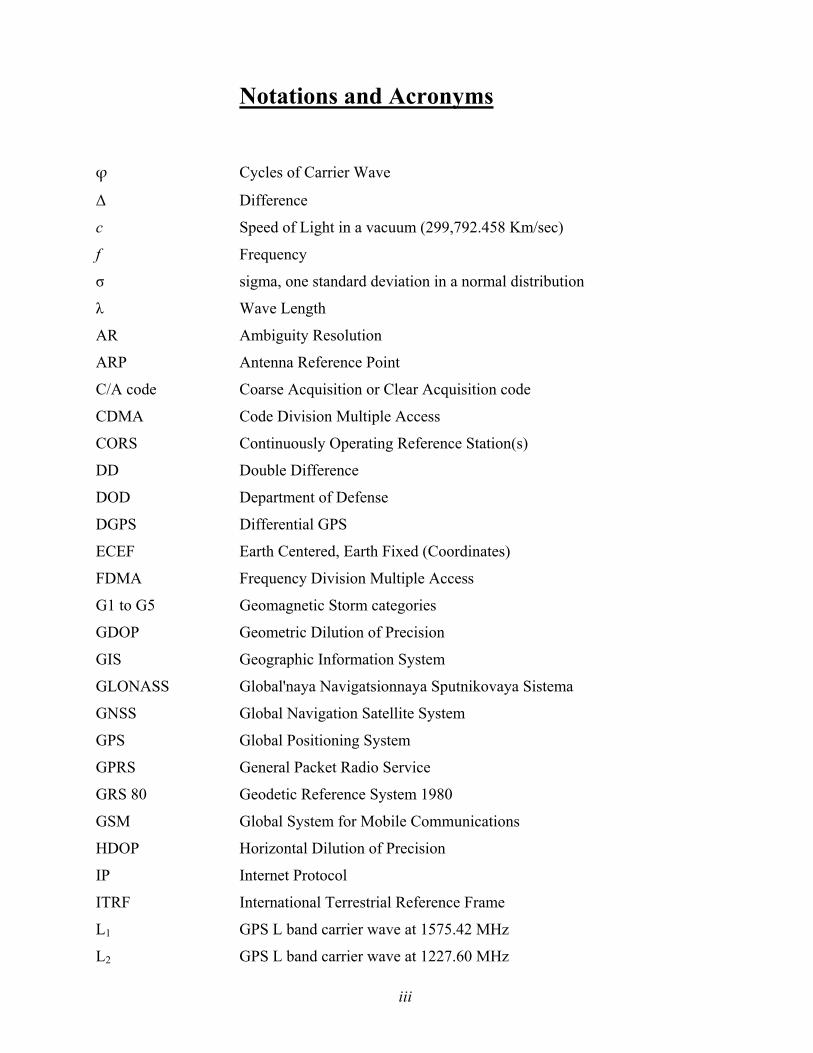
Notations and Acronyms

ϕ Cycles of Carrier Wave

Δ Difference

c Speed of Light in a vacuum (299,792.458 Km/sec)

f Frequency

σ sigma, one standard deviation in a normal distribution

λ Wave Length

AR Ambiguity Resolution

ARP Antenna Reference Point

C/A code Coarse Acquisition or Clear Acquisition code

CDMA Code Division Multiple Access

CORS Continuously Operating Reference Station(s)

DD Double Difference

DOD Department of Defense

DGPS Differential GPS

ECEF Earth Centered, Earth Fixed (Coordinates)

FDMA Frequency Division Multiple Access

G1 to G5 Geomagnetic Storm categories

GDOP Geometric Dilution of Precision

GIS Geographic Information System

GLONASS Global'naya Navigatsionnaya Sputnikovaya Sistema

GNSS Global Navigation Satellite System

GPS Global Positioning System

GPRS General Packet Radio Service

GRS 80 Geodetic Reference System 1980

GSM Global System for Mobile Communications

HDOP Horizontal Dilution of Precision

IP Internet Protocol

ITRF International Terrestrial Reference Frame

L1 GPS L band carrier wave at 1575.42 MHz

L2 GPS L band carrier wave at 1227.60 MHz

iv

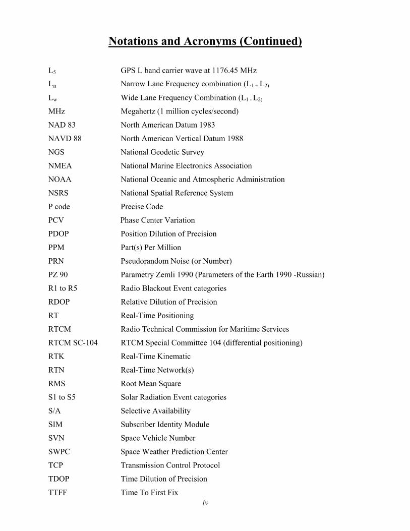
Notations and Acronyms (Continued)

L5 GPS L band carrier wave at 1176.45 MHz

Ln Narrow Lane Frequency combination (L1 + L2)

Lw Wide Lane Frequency Combination (L1 - L2)

MHz Megahertz (1 million cycles/second)

NAD 83 North American Datum 1983

NAVD 88 North American Vertical Datum 1988 NGS National Geodetic Survey

NMEA National Marine Electronics Association

NOAA National Oceanic and Atmospheric Administration

NSRS National Spatial Reference System

P code Precise Code

PCV Phase Center Variation

PDOP Position Dilution of Precision

PPM Part(s) Per Million

PRN Pseudorandom Noise (or Number)

PZ 90 Parametry Zemli 1990 (Parameters of the Earth 1990 -Russian)

R1 to R5 Radio Blackout Event categories

RDOP Relative Dilution of Precision

RT Real-Time Positioning

RTCM Radio Technical Commission for Maritime Services

RTCM SC-104 RTCM Special Committee 104 (differential positioning)

RTK Real-Time Kinematic

RTN Real-Time Network(s)

RMS Root Mean Square

S1 to S5 Solar Radiation Event categories

S/A Selective Availability

SIM Subscriber Identity Module

SVN Space Vehicle Number

SWPC Space Weather Prediction Center

TCP Transmission Control Protocol

TDOP Time Dilution of Precision

TTFF Time To First Fix

v

Notations and Acronyms (Concluded)

UERE User Equivalent Range Error

UHF Ultra High Frequency

UTM Universal Transverse Mercator

VDOP Vertical Dilution of Precision

VHF Very High Frequency

WGS 84 World Geodetic System 1984

1

I. Introduction

These user guidelines are intended to provide a practical method to obtain consistent,

accurate three-dimensional positions using classical, single-base real-time (RT) techniques. Due

to the rapidly changing environment of Global Navigation Satellite System (GNSS) positioning,

it is understood that this documentation will be dynamic and would be best served to remain in

digital form. Improvements to GNSS hardware and software, increased wireless communication

capabilities and additional satellite constellations in production or planned will yield

significantly increased capabilities in easier, faster and more accurate data for the RT positioning

world in the near future. These guidelines are not meant to exclude other accepted practices that

users have found to produce accurate results, but will augment the basic knowledge base to

increase confidence in RT positioning.

Classical (single-base) Real-Time Kinematic (RTK) positioning or “RT” positioning as

commonly shortened, is a powerful technology employing GNSS technology to produce and

collect three-dimensional (3-D) positions relative to a fixed (stationary) base station with

expected relative accuracies in each coordinate component on the order of a centimeter, using

minimal epochs of data collection. Baseline vectors are produced from the antenna phase center

(APC) of a stationary base receiver to the APC of the rover antenna using the Earth-Centered,

Earth-Fixed (ECEF) X,Y,Z Cartesian coordinates of the World Geodetic System 1984 (WGS 84)

datum, which is the reference frame in which the Department of Defense (DoD) Navstar Global

Positioning System (GPS) system broadcast orbits are realized (differential X,Y,Z vectors in

other reference frames would be possible if different orbits were used). Some current technology

may also incorporate the Russian Federation Global'naya Navigatsionnaya Sputnikovaya Sistema

(GLONASS) constellation into the computations, whose orbits are defined in the Parametry

Zemli 1990 (Parameters of the Earth 1990- PZ 90.02) datum. The coordinates of the point of

interest at the rover position are then obtained by adding the vector (as a difference in Cartesian

coordinates) to the station coordinates of the base receiver, and applying the antenna height

above the base station mark and also the height of the rover pole. Usually, the antenna reference

point (ARP) is used as a fixed vertical reference. Phase center variation models, which include a

horizontal and vertical offset constant, are typically applied in the firmware to position the

electrical phase center of the antenna, which varies by satellite elevation and azimuth.

Because of the variables involved with RT however, the reliability of the positions

obtained are much harder to verify than static or rapid static GNSS positioning. The myriad of

2

variables involved require good knowledge and attention to detail from the field operator.

Therefore, experience, science and art are all part of using RT to its best advantage.

RT positioning of important data points can not be done reliably without some form of

redundancy. As has been shown in the NOAA Manual NOS NGS-58 document “GPS Derived

Ellipsoid Heights” (Zilkoski, et. al., 1997), and NOAA Manual NOS NGS-59 draft document

“GPS Derived Orthometric Heights” (Zilkoski, et. al., 2005), GNSS positions can be expected to

have more accurate values when one position that is obtained at a particular time of day is

averaged with a redundant position obtained at a time staggered by 3 or 4 hours. The different

satellite geometry commonly produces different results at the staggered times. The position, all

other conditions being equal, is usually most accurately obtained by simple averaging of the two

(or more) positions thus obtained. Redundant observations are covered in the Accuracy Classes

of the Field Procedures section, where most of the RT Check List items, found below, are also

discussed.

An appreciation of the many variables involved with RT positioning will result in better

planning and field procedures. In the coming years when a modernized GPS constellation and a

more robust GLONASS constellation will be joined by Compass (China), Galileo (European

Union) and possibly other GNSS, there could be in excess of 115 satellites accessible. Accurate,

repeatable positions could become much easier at that time.

NOTES: The term “user” in this document refers to a person who uses RT GNSS

surveying techniques and/or analyzes RT GNSS data to determine three dimensional position

coordinates and metadata using RT methods.

Outside of the Summary sections, important concepts or procedures are designated with

an asterisk, italicized, bolded and underlined, e.g., * Redundancy is critical for important point

positions using RT

A Typical RT Checklist

Knowledge of these concepts covered in the following sections of this document is necessary for expertise at the rover: • PDOP • Multipath • Baseline RMS • Number of satellites • Elevation mask (or cut-off angle) • Base accuracy- datum level, local level • Base security

3

• Redundancy, redundancy, redundancy • PPM – iono, tropo models, orbit errors • Space weather- ‘G”, ‘S”, “R” levels • Geoid quality • Calibration • Bubble adjustment • Latency, update rate • Fixed and float solutions

4

II. Equipment A typical current-configured classical RT set up might use the following equipment: BASE:

1 - dual frequency + GLONASS GNSS base receiver

1- dual frequency + GLONASS ground plane and/or choke ring antenna

1- GNSS antenna cable

1- fixed height tripod

1- lead-acid battery with power lead to receiver. (Note: typical power input level on GNSS

receivers is in the range of 10.5 volts – 28 volts. Users frequently use a 12 volt lawn tractor

battery to keep the carrying weight down.)

Data transmission can be done by one of the following:

a) Broadcast Radio

UHF (0.3 GHz – 3.0 GHz) = 25 watt- 35 watt base radio, Federal Communications Commission

(FCC) licensed two to four channels, lead acid battery, power cable, antenna mast, antenna tripod

or mount for base tripod, data cable. Range is typically 5 km - 8 km (3 miles -5 miles)

* Regardless of the type of external battery used, it should supply at least 12 volts and should

be fully charged. An underpowered battery can severely limit communication range.

Note: A full-size whip antenna option will enhance communications. It can produce a higher

signal to noise ratio and therefore, a longer usable communication range. Also, to greatly extend

range in linear surveys (highways, transmission lines, etc.), a directional antenna for the

broadcast radio should be considered.

Or

b) TCP/IP data connection

CDMA (SIM/Cell/CF card) = wireless data modem, card or phone with static IP address, battery

pack and cable, data cable from receiver or Bluetooth, whip antenna. With the availability of cell

coverage, the range is limited only by the ability to resolve the ambiguities.

5

ROVER:

1-dual frequency GPS + GLONASS integral receiver/antenna, internal batteries

1- carbon fiber rover pole (two sections fixed height), circular level vial

Note: the condition of the rover pole should be straight and not warped or bent in any

manner.

1 – rover pole bipod or tripod with quick release legs

1- data collector, internal battery and pole mount bracket

1- datalink between Receiver and Data Collector, encompassing:

a) Cable

OR

b) Bluetooth wireless connection

Data Reception by one of the following:

a) Internal UHF radio (receive only) with whip antenna

OR

b) CDMA/SIM/Cell/CF card = wireless data modem with static IP address, battery pack

and cable, data cable from receiver or Bluetooth, whip antenna.

Various peripherals, such as laser range finders, inclinometers, electronic compasses, etc. are

also available and may prove useful for various applications.

Note: Single frequency GPS RT is possible. While this application would mean reduced

hardware expense, it also would mean longer initialization times, less robustness, shorter

baselines and would preclude frequency combinations. Thus, L1 RT positioning is not a preferred

solution, and will not be further addressed as a unique application in this document. The general

principles and best methods for RT field work still apply, however, and should be applied for L1

work as well. .

6

The base station should use a ground plane or choke ring antenna, while the rover typically operates with a smaller antenna (usually integrated with the rover receiver) for ease of use.

* Adjust the base and rover circular level vial before every campaign. * As a good practice or if the circular level vial is not adjusted, it is still possible to eliminate the possible plumbing error by taking two locations on a point with the rover pole rotated 180˚ between each location. From SECO ( http://www.surveying.com/tech_tips/details.asp?techTipNo=13 ): ADJUSTMENT OF THE CIRCULAR VIAL: 1. Set up and center bubble as precisely as possible. 2. Rotate center pole 180 degrees. If any part of the bubble goes out of the black circle adjustment is necessary. 3. Move quick release legs until bubble is half way between position one and position two. 4. With a 2.5 mm allen wrench turn adjusting screws until bubble is centered. Recommended

7

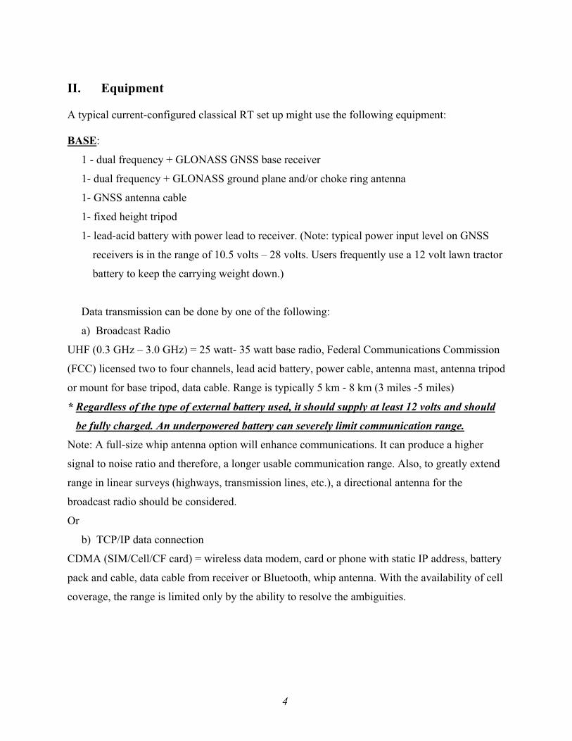
procedure is to tighten the screw that is most in line with the bubble. Caution: very small movements work best. 5. Repeat until bubble stays entirely within circle. A rover pole with an adjusted standard 40 minute vial located about midpoint of the length should introduce a maximum leveling error of no more than 2.5 mm (less than 0.01 feet). It should be noted that 10 minute vials are available. Diagram II-1 - Typical circular vial assembly for the Rover pole TYPICAL RT SET UPS

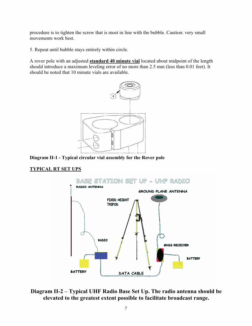
Diagram II-2 – Typical UHF Radio Base Set Up. The radio antenna should be elevated to the greatest extent possible to facilitate broadcast range.

8

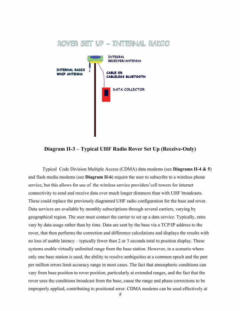
Diagram II-3 – Typical UHF Radio Rover Set Up (Receive-Only)

Typical Code Division Multiple Access (CDMA) data modems (see Diagrams II-4 & 5)

and flash media modems (see Diagram II-6) require the user to subscribe to a wireless phone

service, but this allows for use of the wireless service providers’cell towers for internet

connectivity to send and receive data over much longer distances than with UHF broadcasts.

These could replace the previously diagramed UHF radio configuration for the base and rover.

Data services are available by monthly subscriptions through several carriers, varying by

geographical region. The user must contact the carrier to set up a data service. Typically, rates

vary by data usage rather than by time. Data are sent by the base via a TCP/IP address to the

rover, that then performs the correction and difference calculations and displays the results with

no loss of usable latency – typically fewer than 2 or 3 seconds total to position display. These

systems enable virtually unlimited range from the base station. However, in a scenario where

only one base station is used, the ability to resolve ambiguities at a common epoch and the part

per million errors limit accuracy range in most cases. The fact that atmospheric conditions can

vary from base position to rover position, particularly at extended ranges, and the fact that the

rover uses the conditions broadcast from the base, cause the range and phase corrections to be

improperly applied, contributing to positional error. CDMA modems can be used effectively at

9

extended ranges in RT networks (RTN) where the atmospheric and orbital errors are interpolated

to the site of the rover. Cell phones and stand alone Subscriber Identity Module (SIM) cards (see

Diagram II-7) in Global System for Mobile Communication (GSM) networks use similar

methods as CDMA data modems to send data. Many current GNSS receivers have integrated

communication modules.

Rather than communicating with a dynamic address as is the case in many internet

scenarios, static IP addresses provide a reliable connection and are the recommended

communication link configuration. Static addresses are linked with the same address every time

the data modems connect and are not in use when there is no connection. However, there is a

cost premium for this service. Contact the wireless service provider for the actual rates.

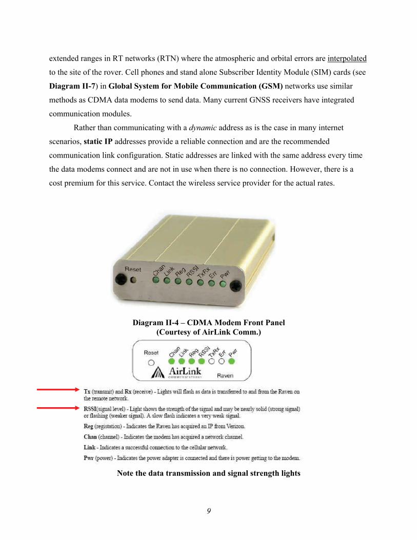
Diagram II-4 – CDMA Modem Front Panel

(Courtesy of AirLink Comm.)

Note the data transmission and signal strength lights

10

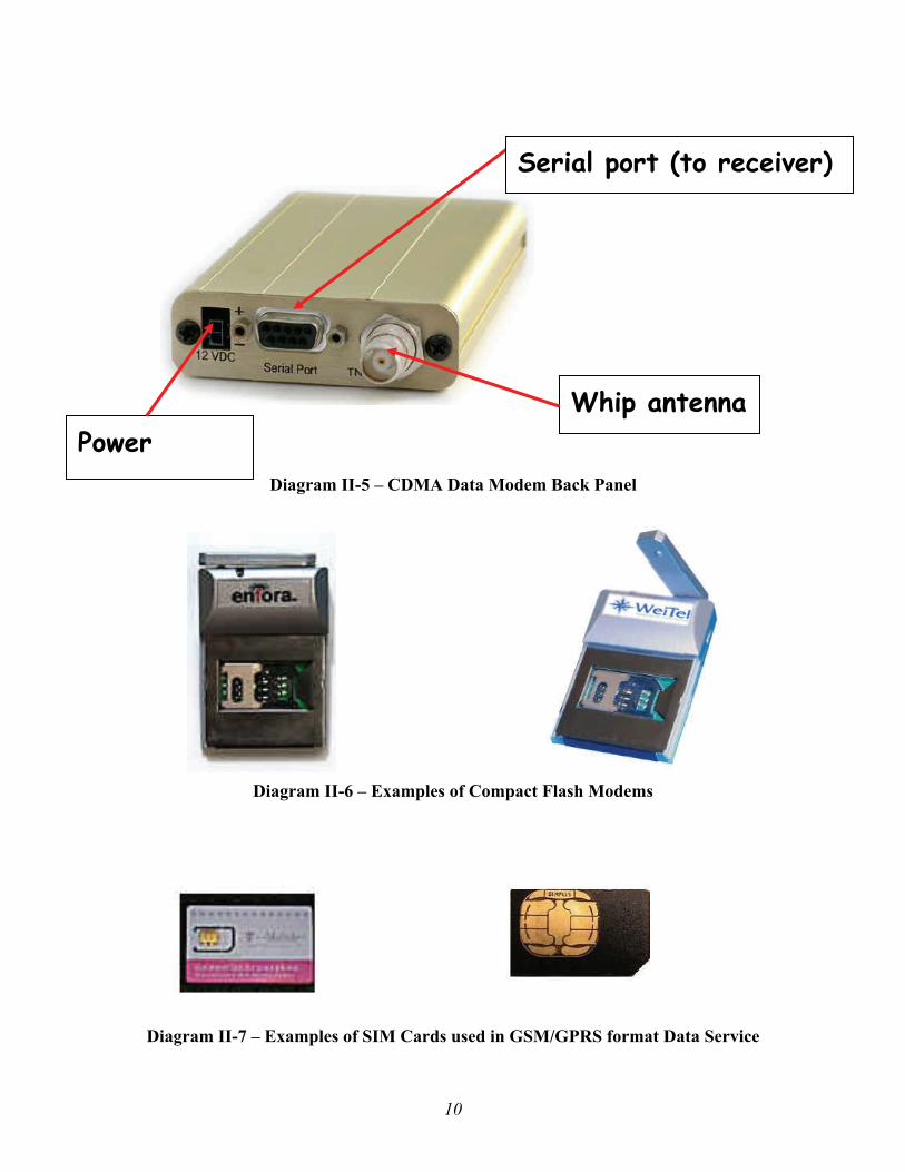
Diagram II-5 – CDMA Data Modem Back Panel

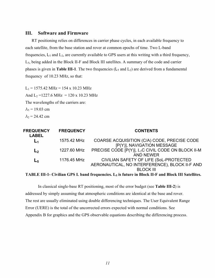
Diagram II-6 – Examples of Compact Flash Modems

Diagram II-7 – Examples of SIM Cards used in GSM/GPRS format Data Service

Whip antenna Power

Serial port (to receiver)

11

III. Software and Firmware

RT positioning relies on differences in carrier phase cycles, in each available frequency to

each satellite, from the base station and rover at common epochs of time. Two L-band

frequencies, L1 and L2, are currently available to GPS users at this writing with a third frequency,

L5, being added in the Block II-F and Block III satellites. A summary of the code and carrier

phases is given in Table III-1. The two frequencies (L1 and L2) are derived from a fundamental

frequency of 10.23 MHz, so that:

L1 = 1575.42 MHz = 154 x 10.23 MHz

And L2 =1227.6 MHz = 120 x 10.23 MHz

The wavelengths of the carriers are: λ1 = 19.03 cm

λ2 = 24.42 cm

FREQUENCY

LABEL FREQUENCY CONTENTS

L1 1575.42 MHz COARSE ACQUISITION (C/A) CODE, PRECISE CODE [P(Y)], NAVIGATION MESSAGE

L2 1227.60 MHz PRECISE CODE [P(Y)], L2C CIVIL CODE ON BLOCK II-M AND NEWER

L5 1176.45 MHz CIVILIAN SAFETY OF LIFE (SoL-PROTECTED AERONAUTICAL, NO INTERFERENCE), BLOCK II-F AND

BLOCK III TABLE III-1- Civilian GPS L band frequencies. L5 is future in Block II-F and Block III Satellites.

In classical single-base RT positioning, most of the error budget (see Table III-2) is

addressed by simply assuming that atmospheric conditions are identical at the base and rover.

The rest are usually eliminated using double differencing techniques. The User Equivalent Range

Error (UERE) is the total of the uncorrected errors expected with normal conditions. See

Appendix B for graphics and the GPS observable equations describing the differencing process.

12

ERROR VALUE Ionosphere 4.0 METERS Ephemeris 2.1 METERS

Clock 2.1 METERS Troposphere 0.7 METERS

Receiver 0.5 METERS Multipath 1.0 METERS TOTAL 10.4 METERS

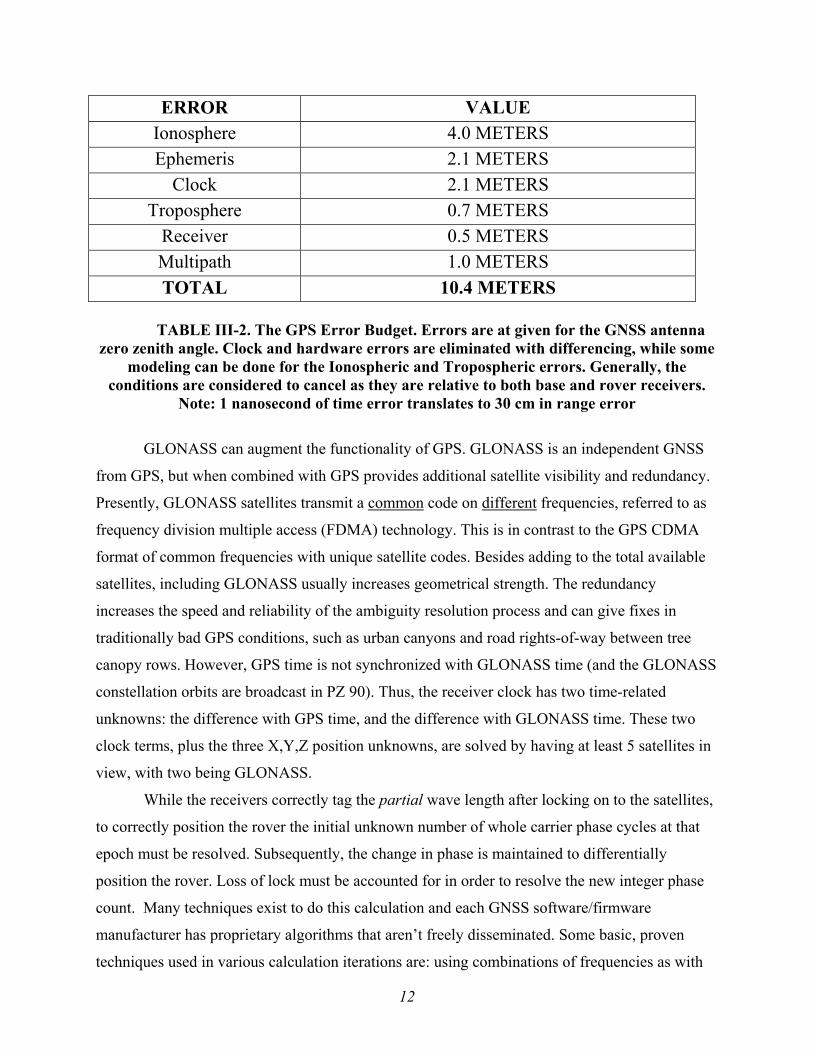
TABLE III-2. The GPS Error Budget. Errors are at given for the GNSS antenna

zero zenith angle. Clock and hardware errors are eliminated with differencing, while some modeling can be done for the Ionospheric and Tropospheric errors. Generally, the

conditions are considered to cancel as they are relative to both base and rover receivers. Note: 1 nanosecond of time error translates to 30 cm in range error

GLONASS can augment the functionality of GPS. GLONASS is an independent GNSS

from GPS, but when combined with GPS provides additional satellite visibility and redundancy.

Presently, GLONASS satellites transmit a common code on different frequencies, referred to as

frequency division multiple access (FDMA) technology. This is in contrast to the GPS CDMA

format of common frequencies with unique satellite codes. Besides adding to the total available

satellites, including GLONASS usually increases geometrical strength. The redundancy

increases the speed and reliability of the ambiguity resolution process and can give fixes in

traditionally bad GPS conditions, such as urban canyons and road rights-of-way between tree

canopy rows. However, GPS time is not synchronized with GLONASS time (and the GLONASS

constellation orbits are broadcast in PZ 90). Thus, the receiver clock has two time-related

unknowns: the difference with GPS time, and the difference with GLONASS time. These two

clock terms, plus the three X,Y,Z position unknowns, are solved by having at least 5 satellites in

view, with two being GLONASS.

While the receivers correctly tag the partial wave length after locking on to the satellites,

to correctly position the rover the initial unknown number of whole carrier phase cycles at that

epoch must be resolved. Subsequently, the change in phase is maintained to differentially

position the rover. Loss of lock must be accounted for in order to resolve the new integer phase

count. Many techniques exist to do this calculation and each GNSS software/firmware

manufacturer has proprietary algorithms that aren’t freely disseminated. Some basic, proven

techniques used in various calculation iterations are: using combinations of frequencies as with

13

wide laning, narrow laning, and iono free, Kalman filtering, and single/double/triple

differencing. These will be briefly discussed in this section to give the user an appreciation of the

complexity of calculations being done at the rover receiver and being displayed in the data

collector, initially in typically under 10 seconds and with only a second (or perhaps up to three

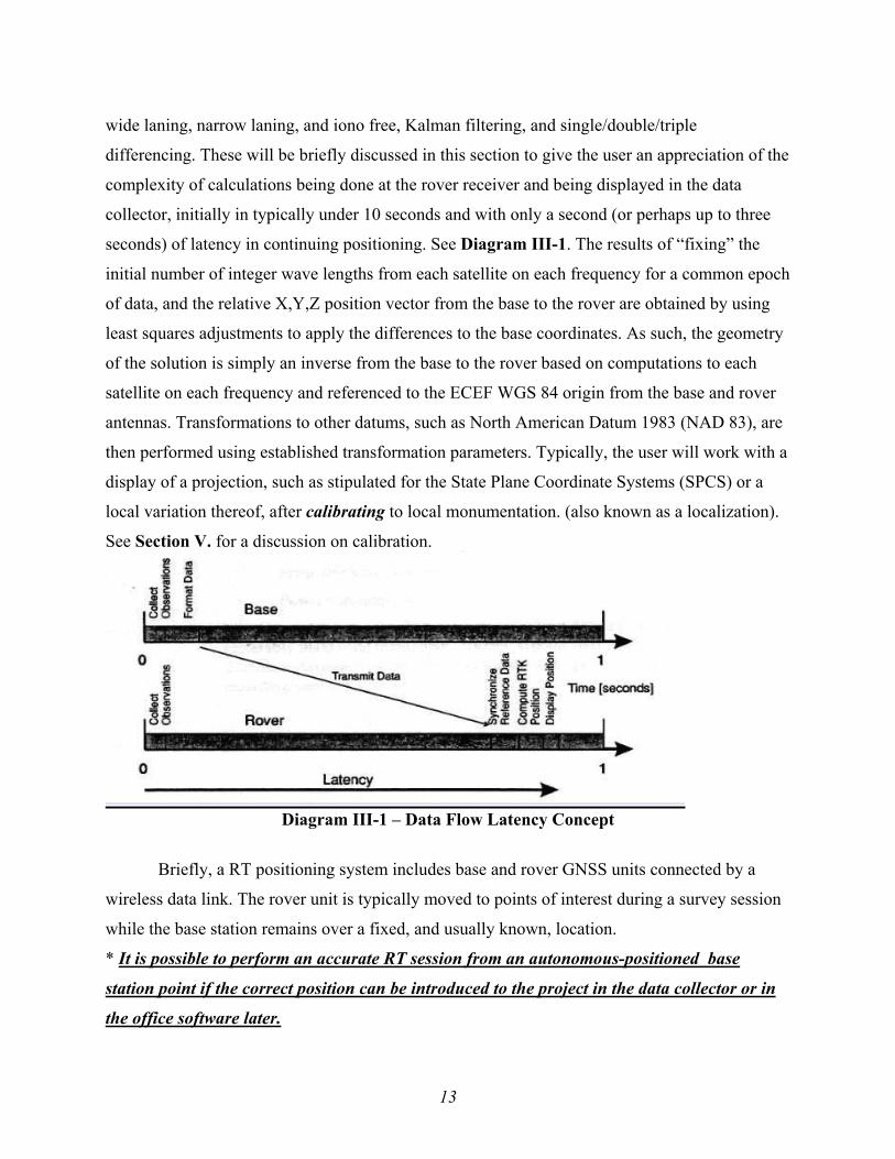
seconds) of latency in continuing positioning. See Diagram III-1. The results of “fixing” the

initial number of integer wave lengths from each satellite on each frequency for a common epoch

of data, and the relative X,Y,Z position vector from the base to the rover are obtained by using

least squares adjustments to apply the differences to the base coordinates. As such, the geometry

of the solution is simply an inverse from the base to the rover based on computations to each

satellite on each frequency and referenced to the ECEF WGS 84 origin from the base and rover

antennas. Transformations to other datums, such as North American Datum 1983 (NAD 83), are

then performed using established transformation parameters. Typically, the user will work with a

display of a projection, such as stipulated for the State Plane Coordinate Systems (SPCS) or a

local variation thereof, after calibrating to local monumentation. (also known as a localization).

See Section V. for a discussion on calibration.

Diagram III-1 – Data Flow Latency Concept

Briefly, a RT positioning system includes base and rover GNSS units connected by a

wireless data link. The rover unit is typically moved to points of interest during a survey session

while the base station remains over a fixed, and usually known, location.

* It is possible to perform an accurate RT session from an autonomous-positioned base

station point if the correct position can be introduced to the project in the data collector or in

the office software later.

14

The autonomous base position is usually taken by selecting the position displayed after

the coordinates “settle down” or start to show less variation from interval to interval- typically 30

seconds or less. Since the rover-generated positions are the result of a vector relative to the base

station, the translation of the autonomous base position to a known position simply shifts the 3-D

vectors to originate at the new coordinates and the field firmware or office software updates the

RT positions accordingly.

The base antenna should be located to optimize a clear view of the sky (Meyer, et al

2002).

*In fact, it is much better to establish a new, completely open sky view site for the base than it

is to try to occupy an existing reliable, well known monument with a somewhat obscured sky

view.

Processing is based on common satellites, and the fact that the rover will usually be in

varying conditions of obstruction to the sky means that it will not always be locked on the total

available satellites. Therefore, the base antenna site must be optimized to look at all the possible

satellites. The rover antenna will often be obstructed by trees or buildings in such a way that the

signals are interrupted and a reinitialization process is performed. Each rover project site could

conceivably use a different subset of the total in view constellation because of the obstructions.

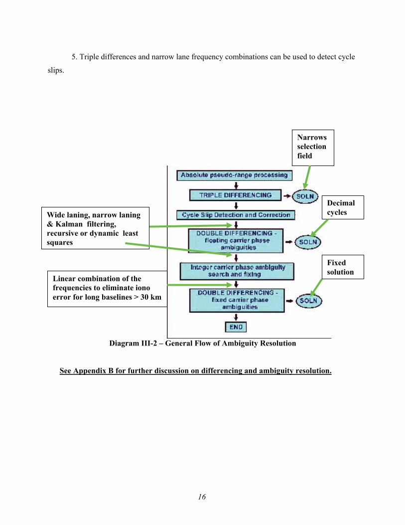
Explained in an extremely general way, the rover might progress through the following

algorithms in an iterative process to get a fixed ambiguity resolution. (Also, see Diagram III-2):

1. Use pseudorange and carrier phase observables to estimate integer ambiguities.

Multipath can cause pseudorange noise which will limit this technique. Typically, this can

achieve sub meter positions. Kalman filtering or recursive least square selection sets can aid in

narrowing the selection set.

2. Achieve a differential float ambiguity solution (this is a decimal carrier phase count,

rather than a whole number of cycles). Estimates are run through measurement noise reduction

filters. Differencing reduces or eliminates satellite clock errors, receiver clock errors, satellite

hardware errors, receiver hardware errors, and cycle slips.

3. Integer ambiguity search is started. Frequency combinations narrow the field of

candidates. The more satellites, the more robust the integer search:

The wide lane wave length, Lw, is the difference of the two GPS frequencies, L1-L2. So,

“c” (speed of light) ÷ (1575.42 MHz – 1227.60 MHz) or 299,792.458 Km/sec ÷ 347.82 MHz =

0.862 m effective wave length. This longer wave length is more readily resolved compared to the

15

L1 frequency wave length of 0.190 m, or L2 frequency wave length of 0.240 m. However, the

wide lane combination adds about 6 times the “noise” to the observable, and about 1.28 times to

the ionospheric effect.

The narrow lane wave length, Ln, is the sum of the two GPS frequencies, L1 + L2.

So, c (speed of light) ÷ (1575.42 MHz + 1227.60 MHz) or 299,792.458 Km/sec

÷ 2803.02 MHz = 0.107 m wave length. The narrow wave length makes the ambiguity hard to

resolve for this combination, but helps detect cycle slips, compute Doppler frequencies and to

validate the integer resolution.

The “Ionosphere free” or, as commonly called, “L3” linear combination of the

frequencies can eliminate most of the ionosphere error (phase advance, group code delay) in the

observables but shouldn’t be relied on for the final solution for short baselines because of the

additional noise introduced into the solution. The time delay of the signal is proportional to the

inverse of the frequency squared - that is, higher frequencies are less affected by the ionosphere,

and hence the ionospheric time delay for L1 observations (1575.42MHz) is less than for L2

observations (1227.60MHz). The L3 wavelength is 48.44 m. However, the L2 ionospheric error

effect is approximately 1.646 times that of L1 and noise is also increased. Still, double

differenced L3 combinations can provide the most accurate solution on extended baseline

lengths.

4. The integer ambiguity is fixed and initialization of sub-centimeter level positioning

begins. Covariance matrices can be stored in certain rover configurations to enable post

campaign adjustment in the office software (assuming redundancy or baseline connections).

Continual fixed ambiguity analysis is performed at the rover to verify the integer count. Ratio of

the best to next best solution is evaluated. It is interesting to note that the confidence of a correct

integer fix is stated by most GNSS hardware manufacturers at 99.9 percent (even though an

incorrect set of integer ambiguities can appear to the layman to be a better statistical choice!).

RMS values of the solution and vector are produced. Once initialized, a subsequent loss of

initialization and integer search is considerably enhanced when two or more satellites have been

continuously tracked throughout. One or two surviving double-differenced integers bridge over

the loss of initialization. This then significantly reduces the number of potential integer

combinations and speeds a final integer solution, whereas complete loss of lock starts the

ambiguity resolution process over again at step 1.

16

5. Triple differences and narrow lane frequency combinations can be used to detect cycle

slips.

Diagram III-2 – General Flow of Ambiguity Resolution

See Appendix B for further discussion on differencing and ambiguity resolution.

Linear combination of the frequencies to eliminate iono error for long baselines > 30 km

Wide laning, narrow laning & Kalman filtering, recursive or dynamic least squares

Narrows selection field

Decimal cycles

Fixed solution

17

IV. Before Beginning Work

An awareness of the expected field conditions can help produce successful campaigns.

Although the conditions at all rover locations can not be known beforehand- especially for

multipath and obstructions- satellite availability and geometry, space weather, and atmospheric

conditions can be assessed.

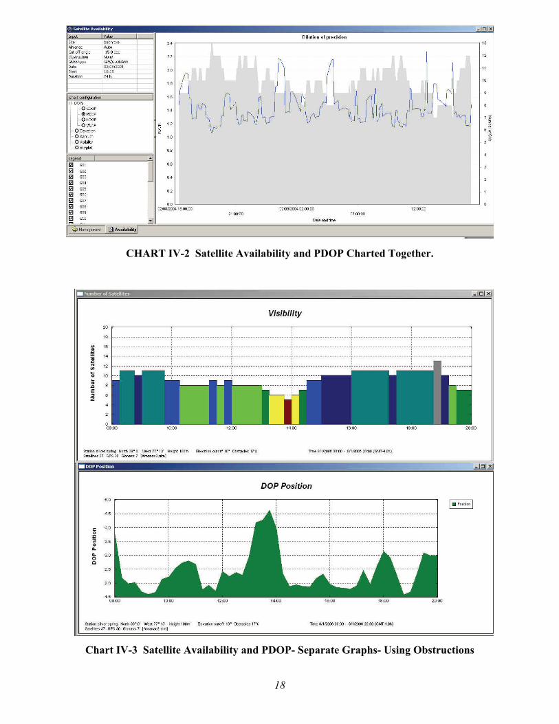
All major GNSS hardware and software providers include a mission planning tool or module

charting the sky plot and path of the satellites, the number of satellites and the different DOP

across a time line (see Charts IV-1, 2 and 3). Additionally, elevation masks and obstructions

can be added to give a realistic picture of the conditions at the base location. The user should

expect that these would be the optimum conditions and those that the rover will experience will

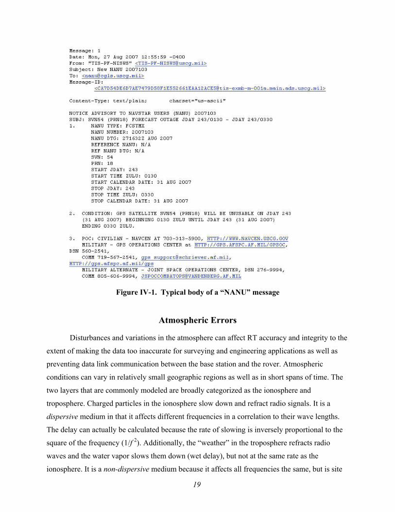
be less than ideal. For current satellite outages, the U.S. Coast Guard sends out a Notice

Advisory to Navstar Users (NANU). Users can subscribe to this free mailing at:

http://cgls.uscg.mil/mailman/listinfo/nanu . See Figure IV-1 for an example.

Atmospheric conditions are difficult to predict and, as a result, the user may expect

occasional surprises in the form of loss of radio communication or inability to initialize to a fixed

position. Predicting atmospheric conditions for any particular area is problematic at best, but the

task of how to approach this problem appears to be underway by space weather scientists and

professionals. GNSS users will benefit by this heightened interest in how space weather affects

our lives. For a wealth of information on the topic the reader is referred to the NOAA Space

Weather Prediction Center (SWPC) web site at: http://www.sec.noaa.gov/

An effort is made herein, however, to summarize some conditions and how we may get timely

information which may affect our RT field work.

Chart IV-1 Typical Satellite Sky Plots –with and without Site Obstructions

18

CHART IV-2 Satellite Availability and PDOP Charted Together.

Chart IV-3 Satellite Availability and PDOP- Separate Graphs- Using Obstructions

19

Figure IV-1. Typical body of a “NANU” message

Atmospheric Errors

Disturbances and variations in the atmosphere can affect RT accuracy and integrity to the

extent of making the data too inaccurate for surveying and engineering applications as well as

preventing data link communication between the base station and the rover. Atmospheric

conditions can vary in relatively small geographic regions as well as in short spans of time. The

two layers that are commonly modeled are broadly categorized as the ionosphere and

troposphere. Charged particles in the ionosphere slow down and refract radio signals. It is a

dispersive medium in that it affects different frequencies in a correlation to their wave lengths.

The delay can actually be calculated because the rate of slowing is inversely proportional to the

square of the frequency (1/f 2). Additionally, the “weather” in the troposphere refracts radio

waves and the water vapor slows them down (wet delay), but not at the same rate as the

ionosphere. It is a non-dispersive medium because it affects all frequencies the same, but is site

20

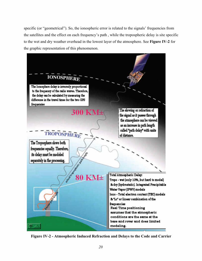
specific (or “geometrical”). So, the ionospheric error is related to the signals’ frequencies from

the satellites and the effect on each frequency’s path , while the tropospheric delay is site specific

to the wet and dry weather overhead in the lowest layer of the atmosphere. See Figure IV-2 for

the graphic representation of this phenomenon.

Figure IV-2 - Atmospheric Induced Refraction and Delays to the Code and Carrier

21

Unlike networked solutions for RT positioning, in classical (single-base) RT positioning

there is minimal atmospheric modeling because it is assumed that both the base station and the

rover are experiencing nearly identical atmospheric conditions. Therefore, the errors will be

relative to both and would not adversely affect the baseline between them as long as baseline

distances are kept relatively short (≤ 20 km) so that atmospheric conditions are not expected to

differ between base and rover. However, a correct ambiguity resolution must be achieved to

provide centimeter-level precision. Atmospheric conditions can cause enough signal “noise” to

prevent initialization or, worse, can result in an incorrect ambiguity resolution. Additionally,

moderate to extreme levels of space storm events as shown on the NOAA Space Weather

Prediction Center (SWPC) Space Weather Scales (see link below) could cause poor, intermittent

or loss of, radio or wireless communication.

Ionospheric Error Discussion

Sun spots (emerging strong magnetic fields) are the prime indicators of solar activity

contributing to increased ionospheric (and possibly tropospheric) disturbance. They are relatively

predictable and run in approximately 11 year cycles. The last minimum was in 2006/2007 and

the next maximum is expected around 2011. During an interval encompassing the solar

maximum, users can expect inability to initialize, loss of satellite communications, loss of

wireless connections and radio blackouts, perhaps in random areas and time spans. Therefore, it

is critical to understand these conditions. The charged particles in the ionosphere affect radio

waves proportional to the "total electron content" (TEC) along the wave path. TEC is the total

number of free electrons along the path between the satellite and GNSS receiver. In addition,

TEC varies according to solar and geomagnetic conditions at time of day, geographic location

and season. As we go up the sunspot number scale to the next solar maximum, the effects on

GNSS signals will increase and there will be more problems even at mid latitudes which are not

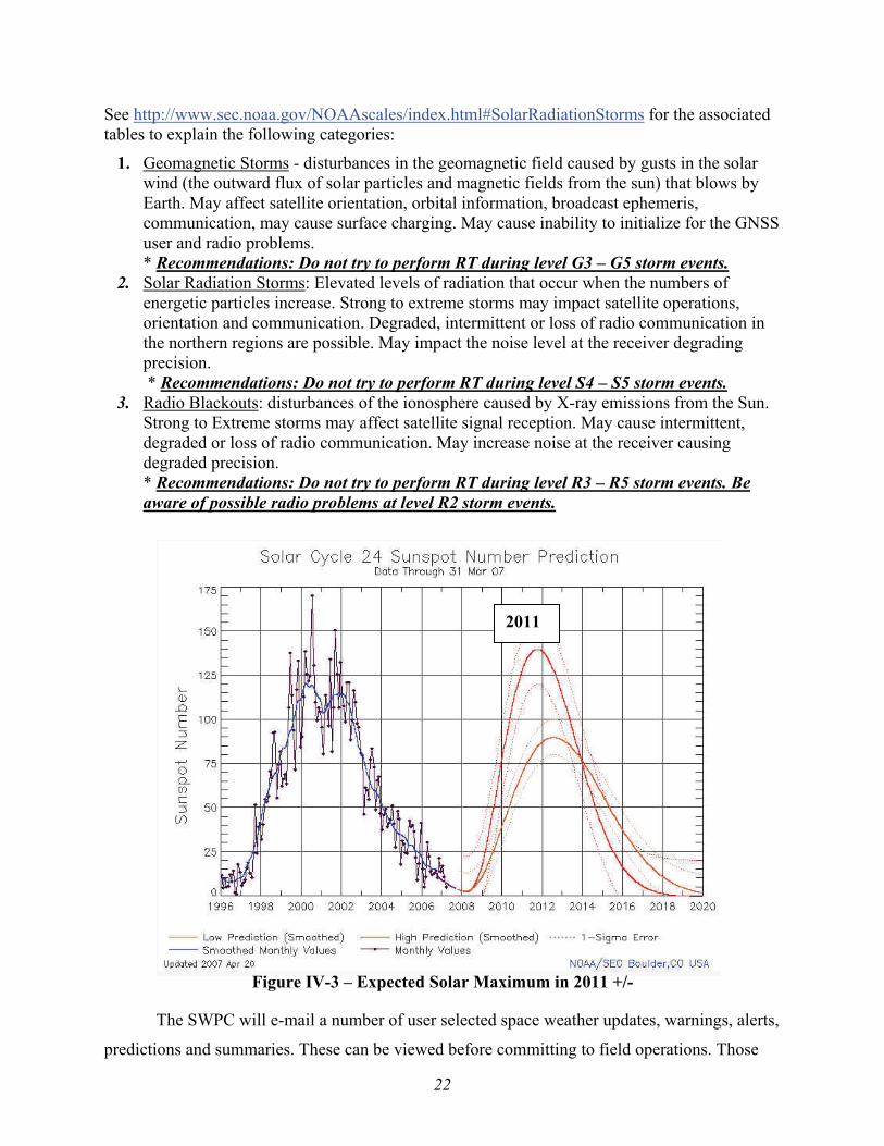
present now. See Figure IV-3 for the plot of the immediate past, present and predicted solar

cycle.

The following is a summary of space weather conditions and how they may impact RT

users as extracted from NOAA’s SWPC. The SWPC provides warnings in three different

categories: Geomagnetic Storm, Solar Radiation Storm and Radio Blackout. Each of these has a

range from mild to severe, such as G1(mild) through G5(severe), and S1-S5 and R1-R5

inclusive.

22

See http://www.sec.noaa.gov/NOAAscales/index.html#SolarRadiationStorms for the associated tables to explain the following categories:

1. Geomagnetic Storms - disturbances in the geomagnetic field caused by gusts in the solar wind (the outward flux of solar particles and magnetic fields from the sun) that blows by Earth. May affect satellite orientation, orbital information, broadcast ephemeris, communication, may cause surface charging. May cause inability to initialize for the GNSS user and radio problems. * Recommendations: Do not try to perform RT during level G3 – G5 storm events.

2. Solar Radiation Storms: Elevated levels of radiation that occur when the numbers of energetic particles increase. Strong to extreme storms may impact satellite operations, orientation and communication. Degraded, intermittent or loss of radio communication in the northern regions are possible. May impact the noise level at the receiver degrading precision. * Recommendations: Do not try to perform RT during level S4 – S5 storm events.

3. Radio Blackouts: disturbances of the ionosphere caused by X-ray emissions from the Sun. Strong to Extreme storms may affect satellite signal reception. May cause intermittent, degraded or loss of radio communication. May increase noise at the receiver causing degraded precision. * Recommendations: Do not try to perform RT during level R3 – R5 storm events. Be aware of possible radio problems at level R2 storm events.

Figure IV-3 – Expected Solar Maximum in 2011 +/-

The SWPC will e-mail a number of user selected space weather updates, warnings, alerts,

predictions and summaries. These can be viewed before committing to field operations. Those

2011

23

interested should submit the requests from the SWPC web site as referenced above. However, it

must be remembered that conditions change rapidly and can not always be predicted, even short

term. The user can be aware of these conditions if field problems arise so that error sources can

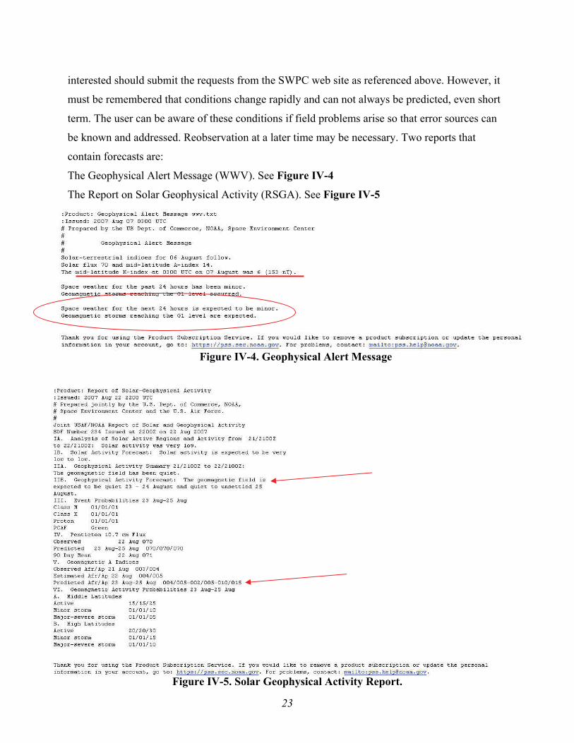
be known and addressed. Reobservation at a later time may be necessary. Two reports that

contain forecasts are:

The Geophysical Alert Message (WWV). See Figure IV-4

The Report on Solar Geophysical Activity (RSGA). See Figure IV-5

Figure IV-4. Geophysical Alert Message

Figure IV-5. Solar Geophysical Activity Report.

24

Tropospheric Delay Discussion While tropospheric models are available as internal program components, they do not

account for the highly variable local fluctuations in the wet and dry components. The dry, or

hydrostatic component comprises 90 percent of the troposphere and can be well modeled

(approximately 1 percent error). The wet component as water vapor is the other 10 percent, but

can not be easily modeled (10 percent – 20 percent error). Position calculation residuals result

from modeling the corrections at the base versus using the “real” conditions at the rover. Also, it

should be stated that tropospheric correction models introduce approximately 1mm per meter of

height difference between base and rover in delay errors, which is probably not being modeled

[Beutler, et al., 1989]. These contribute to a distance dependent error (along with the ionospheric

conditions and ephemerides, which also decorrelate with distance from the base). The

tropospheric error mainly contributes to the error in height.

* The single most important guideline to remember about the weather with RT

positioning is to never perform RT in obviously different conditions from base to rover.

This would include storm fronts, precipitation, temperature or atmospheric pressure. Either wait

for the conditions to become homogenous or move the base to a position that has similar

conditions to the rovers intended location(s).

In RT positioning there exists a distance correlated error factor, i.e. the further apart the

two receivers, the greater the inconsistent atmospheric conditions and orbital variations will

affect a computed precision. These residual biases arise mainly because the satellite orbit errors

and the atmospheric biases are not eliminated when calculating a position using the observations

from two receivers. Their effect on relative position determination is greater for long baselines

than for short baselines. Most GNSS hardware manufacturers specify a 1 part per million

(ppm) constant to account for this error (i.e. 1 mm/km). Therefore, this is correlated to the

baseline distance. The signals traveling close to the horizon have the longest path through the

atmosphere and therefore the errors introduced are hardest to correct, introducing the most noise

to the position solution. Unfortunately, by raising the mask even higher than 15˚, the loss of data

becomes a problem for the integrity of the solution and may contribute to higher than desired

PDOP.

* It is helpful to partially mitigate the worst effects of atmospheric delay and refraction by setting an elevation mask( cut off angle) of 12°- 15° to block the lower satellites signals which have the longest run through the atmosphere.

25

V. Field Procedures The control of a classical RT positioning survey is always in the hands of the rover. Because of the variables involved with RT therefore, this section is the core to achieving accurate positions from RT. The following are all terms that must be understood and/or monitored by RTK field technicians:

Accuracy versus Precision

Multipath

Position Dilution of Precision (PDOP)

Root Mean Square (RMS)

Site Calibrations (a.k.a. Localizations)

Latency

Signal to Noise Ratio (S/N or C/N0)

Float and Fixed Solutions

Elevation Mask

Geoid Model

Additionally, the following are concepts that should be understood.

Please see the RT positioning glossary (herein) for brief definitions:

Carrier Phase

Code Phase

VHF/UHF Radio Communication

CDMA/SIM/Cellular TCP/IP Communication

Part Per Million (PPM) Error

WGS 84 versus NAD 83

GPS and GLONASS Constellations

Almost all of the above were facets of satellite positioning that “the GPS guru” back in

the office worried about with static GPS positioning. Field technicians usually worried about

getting to the station on time, setting up the unit, pushing the ON button and filling out a simple

log sheet. Plenty of good batteries and cables were worth checking on also. While the field tech

still needs plenty of batteries and cables, she or he now needs to have an awareness of all the

important conditions and variables in order to get good RT results – because in RT positioning,

“It Depends” is the answer to most questions.

26

Accuracy versus Precision An important concept to understand when positioning to a specified quality is the

difference between “accuracy” and “precision”. The actual data collection or point stake out is

displayed in the data collector based on a system precision which shows the spread of the results

(RMS) at a certain confidence level and the calculated 2-D and height (horizontal and vertical)

solution relative to the base station in the user’s reference frame. In other words, it is the ability

to repeat a measurement internal to the measurement system. Accuracy, on the other hand, is the

level of the alignment to what is used as a datum, i.e. to externally defined standards. The

“realization” of a datum is its physical, usable manifestation. Therefore, it can be “realized” by

published coordinates on passive monumentation such as is found in the NGS Integrated Data

Base (NGS IDB), by locally set monuments or by assumed monuments. Accuracy can also be

from alignment to active monumentation such as from the NGS Continuously Operating

Reference Station (CORS) network or a local RTN. The geospatial professional must make the

choice of what is held as “truth” for the data collection. It is expected that the same datum,

realized at the same control system monumentation, is held from the design stage through

construction for important projects. A professional surveyor, or other qualified geospatial

professional, should be involved to assess the datum and its realization for any application. The

alignment to the selected truth shows the accuracy of survey. For example, as stated in draft

document for GPS derived orthometric heights (Zilkoski, et al, 2005), accuracy at the datum

level (North American Vertical Datum of 1988 - NAVD 88), is less accurate then the local

accuracy between network stations. Ties were shown at a 5 cm level to the national datum, while

local accuracies can be achieved to the 2 cm level. Subsequent project work done with classical

surveying instruments (but still in NAVD 88) could be done at much higher precision at the

millimeter level, but the accuracy of the tie to the national datum is still 5 cm at best. Because

RT positions are being established without the benefit of an internal network adjustment,

accuracy at any one point is an elusive concept. By basing the survey on proven control

monumentation with a high degree of integrity, monitoring the precision as the work proceeds

and checking points with known values before, during and after each RT session, the user can get

a sense of the accuracy achieved. It can be seen that if the base station is correctly set up over a

monument whose coordinates are fully accepted as truth, correct procedures are used, and

environmental conditions are consistent, then the precision shown would indeed indicate project

accuracy. (Remember though, that this is only accuracy within the datum, and does not speak to

the accuracy of the datum itself)

27

Multipath

Multipath error can not be detected in the rover or modeled in the RT processing.

Basically, anything which can reflect a satellite signal can cause multipath and induce error into

a coordinate calculation. When a reflected signal reaches the receiver’s antenna, the path is

interpreted as if it was a direct path from the satellite, even though it really took a longer time by

being reflected. This then would trick the receiver into using the longer time (or therefore, longer

distance) in its solution matrix to resolve the ambiguities for that satellite. This bias in

time/distance introduces noise to the solution (much like a “ghost” on a television with a bad

rabbit ears antenna) and can cause incorrect ambiguity fixes or noisy data (as may be evidenced

by higher than expected RMS). Multipath is cyclical (over 20 minutes -25 minutes typically) and

static occupations can use sophisticated software to model it correctly in post processed mode.

The rapid point positioning techniques of RT prevent this modeling. Trees, buildings, tall

vehicles nearby, water, metal power poles, etc. can be sources of multipath. GNSS RT users

should always be aware of these conditions.

*Areas with probable multipath conditions should not be used for RT positioned

control sites -especially not for a base station position.

Because the typical RT occupation will only be anywhere from a few seconds to a few

minutes, there is not enough time to model the multipath present at any point. Indeed, the

firmware in the rover receiver and data collector will not address this condition and will continue

to display the false precision as if it was not present. Besides contributing to the noise in the

baseline solution, multipath can cause an incorrect integer ambiguity resolution and thus give

gross errors in position- particularly the vertical component. It has been seen to give height errors

in excess of 2 dm because of incorrect ambiguity fixes and noise. Multipath isn’t always

apparent and it’s up to the common sense of the RT user to prevent or reduce its effects. Getting

redundant observations with different satellite geometry might help to mitigate multipath error.

28

Multipath Conditions can cause unacceptable errors by introducing noise and even incorrect ambiguity resolution because of signal delay.

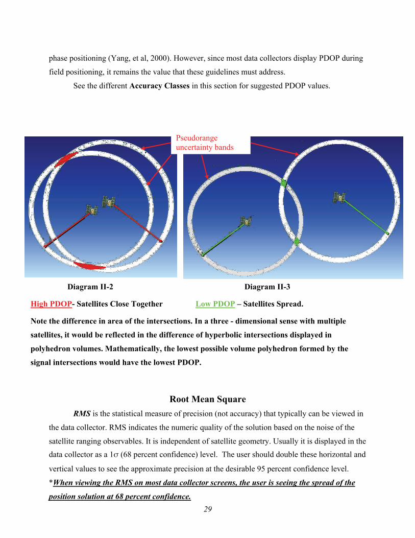
Position Dilution of Precision PDOP is a unitless value reflecting the geometrical configuration of the satellites in

regard to horizontal and vertical uncertainties. Stated in a simplified way, DOP is the ratio of the

positioning accuracy to the measurement accuracy. Error components of the observables are

multiplied by the DOP value to get an error value compounded by the weakness in the

geometrical position of the satellites as can be shown relative to the intersection of their signals.

This is depicted in Diagrams II-2 and 3. Therefore, lower DOP values should indicate better

precision, but cannot be zero, as this would indicate that a user would get a perfect position

solution regardless of the measurement errors. Under optimal geometry with a large numbers of

satellites available (generally 13 or more), PDOP can actually show (usually very briefly) as a

value less than one, indicating that the RMS average of the position error is smaller than the

measurement standard deviation. PDOP is related to horizontal and vertical DOP by:

PDOP2 =HDOP2 + VDOP2. Another DOP value – Relative Dilution of Precision (RDOP) has

been researched as a better indicator for the effects of satellite geometry on differential carrier

29

phase positioning (Yang, et al, 2000). However, since most data collectors display PDOP during

field positioning, it remains the value that these guidelines must address.

See the different Accuracy Classes in this section for suggested PDOP values.

Diagram II-2 Diagram II-3

High PDOP- Satellites Close Together Low PDOP – Satellites Spread.

Note the difference in area of the intersections. In a three - dimensional sense with multiple

satellites, it would be reflected in the difference of hyperbolic intersections displayed in

polyhedron volumes. Mathematically, the lowest possible volume polyhedron formed by the

signal intersections would have the lowest PDOP.

Root Mean Square

RMS is the statistical measure of precision (not accuracy) that typically can be viewed in

the data collector. RMS indicates the numeric quality of the solution based on the noise of the

satellite ranging observables. It is independent of satellite geometry. Usually it is displayed in the data collector as a 1σ (68 percent confidence) level. The user should double these horizontal and

vertical values to see the approximate precision at the desirable 95 percent confidence level.

*When viewing the RMS on most data collector screens, the user is seeing the spread of the

position solution at 68 percent confidence.

Pseudorange uncertainty bands

30

Site Calibrations (a.k.a. Localizations)

Site calibrations should be performed whenever the user wants to constrain the project area

to the realization of a datum at local monumentation. In areas where the control is known to

relate accurately to other monumentation and to the user’s datum, and has been confidently used

[such as is the case with SPCS projections at undisturbed high order stations in the National

Spatial Reference System (NSRS)], the base station can simply occupy one of the trusted control

monuments and begin the RT survey. The alignment to the national datum is known (if the

monument is known to be undisturbed) and the relative accuracy of the control is higher than the

results that could be obtained from the RT survey. However, even working in an NAD 83 SPCS

it obviously does not mean all monuments that are the realization of that datum are to be trusted.

In such cases, and in all cases where other datums or other particular local coordinates or

elevations are to be held, a site calibration should be performed.

*RT calibrations allow the user to transform the coordinates of the control monumentation

positioned by their RT-derived positions in the WGS 84 datum, to the user datum (even if it’s

assumed) as realized by the user’s coordinates on the monuments.

In other words, the user’s firmware is performing a rotation, translation and scale

transformation from the WGS 84 datum realized in the broadcast satellite ephemeris to a local

datum realized on physical monuments visited in the field survey.

Note: GLONASS satellite ephemerides used by the RT survey are transformed from PZ 90

to WGS 84.

Before performing a calibration, the project site should be evaluated and after control

research and retrieval, the monumentation coordinates to be used for the calibration should be

uploaded to the field data collector. * To have confidence in a site calibration, the project site must be surrounded by at least 4 trusted vertical control monuments and 4 trusted horizontal control monuments which to the greatest extent possible, form a rectangle.

The monuments can be both horizontal and vertical control stations, but should be of sufficient

accuracy to be internally consistent to the other calibration control at a level greater than the

required RT project accuracy. Adding more trusted control that meet these criteria will add to

31

confidence in the calibration, especially if they can be spaced throughout the project area. For the

limiting accuracy of RT field work, most GNSS software and hardware manufacturers state their

RT positioning accuracies as 1 cm + 1 ppm horizontal and 2 cm + 1 cm ppm vertical (at the 68 percent or 1σ level). This is further substantiated by ISO testing standards under current

development in ISO/PRF 17123-8. Thus, for a calibration control spacing of 20 km, the

calibration adjustment statistics might be recommended to show less than a 2 cm horizontal

residual and less than a 4 cm vertical residual at a 95 percent confidence (twice the confidence of

the RT work done with 68 percent confidence). Site calibrations can be performed in the field by

a competent RT user and imported into the office GNSS software, or performed in the office

and uploaded to the data collector. The firmware/software will yield horizontal and vertical

residuals which must be reviewed to check for outliers. It can be seen that this is a good way to

assess the relative accuracy of all the existing project control.

*It is critical that all project work is done using the same correct and verified calibration. Different calibrations can result in substantially different position coordinates

Latency

Latency is the delay for the received satellite signal data and correction information at the

base to be wirelessly broadcast, received by the rover radio, transferred to the rover receiver,

have corrections computed and applied for the current common epoch, sent to the data collector

and displayed for the user. The position the user views on the data collector can be up to 5

seconds old, but typically an effective latency of 2 or 3 seconds is the maximum experienced.

The data can be updated (or sampled) at a much higher rate, say 5 Hz, but the usable coordinate

is usually produced at .33 to 1 Hz.

Signal to Noise Ratio Receivers must process GNSS signals through background noise. This can be from

atmospheric conditions, radio frequency interference or from hardware circuitry. Since GNSS

signals are relatively weak (the total transmitted power from a satellite is less than 45 w!), it is

important to use data that doesn’t fall below acceptable noise levels (a common level is given as

30 dB). Signal-to-noise ratio (SNR) can be an indicator of multipath if other contributing noise

factors, such as antenna gain, can be removed. The signal-to-noise ratio compares the level of the

GNSS signal to the level of background noise. The higher the ratio, the less obtrusive is the

32

background noise. We usually refer to the signal to noise ratio by the abbreviation S/N or SNR

(or sometimes carrier signal amplitude over 1 Hz = C/N0). It is usually based on a decibel (dB)

base 10 logarithmic scale. Most GNSS firmware in the data collectors are capable of displaying

this value on some kind of scale. Unfortunately, unlike GPS code and phase observables, a

standard practice for computing and reporting SNR has not been established. Thus, the value and

the units used for reporting it differ among manufacturers. At this time it is not possible to give

independent numerical values to the SNR for all receiver brands. Therefore, the only

recommendation made is to refer to each manufacturer’s reference material and support system

to try to ascertain a minimum SNR (or C/N0 ). Some considerations to ponder include:

1. NMEA message type GSV supposedly shows C/N0 in dB.

2. Current Rinex 2.10+ versions allow the SNR to be reported in the original observations.

3. Comparison of SNR between satellites can show the source of the cleanest data.

See Langley (1997)

Float and Fixed Ambiguities In the quest to resolve the ambiguous number of whole carrier cycles between each

satellite and each GNSS receiver’s antenna, which will be added to the partial cycle which the

receivers’ record after locking on to the satellites, many iterations of least squares adjustments

are performed. A first list of candidates produces a set of partial whole cycle counts, that is, a

decimal number to each satellite for each frequency. This decimal cycle count is said to be the

“float” solution – one that still has not yet forced the number of whole cycles to take an integer

value. Usually while stationary, the positional RMS and horizontal and vertical precisions will

slowly decrease as the rover receiver iterates solutions. The user will see these indicators go from

several meters down to submeter. Sometimes the solution rapidly goes to fixed and these

iterations are not seen.

*The user must be aware of the solution state and should wait until the solution is displayed as

fixed before taking RT locations

As soon as the solution is “fixed” and the best initial whole number of cycles has been

solved, the data collector will display survey grade position precision at the sub-centimeter level.

33

Elevation Mask

Because GNSS satellite signals have the longest paths through the atmosphere at low

elevations from the horizon, it is advantageous to set a cut off angle to eliminate this noisy data.

The base station and rover are typically set to an elevation mask of between 12˚ and 15˚. In

addition to this mask, individual satellites can be switched to inactive in the firmware. This may

be of some advantage where there are many satellites available but due to obstructions, a certain

satellite may be at a higher noise level and be a detriment to a robust solution. Typically, the

satellites can be viewed graphically in a data collector screen.

The Hybrid Geoid Model

The NGS has for a number of years provided a hybrid geoid model from which users of

GPS could take the field-produced NAD 83 ellipsoid heights and compute NAVD 88

orthometric heights in the continental USA and Alaska. The hybrid geoid model gives a distance

or separation between the two surfaces defined as NAD 83 and NAVD 88. Although this model

has been consistently updated, densified and improved, residuals in interpolation based on the

resolution of the model are to be expected. As of this writing, users can expect relative elevation

accuracy of 4.8 cm (2 sigma) internal accuracy, which includes GPS observation error. Error in

the geoid is expected at about 2 cm (2 sigma) at about 10 km wavelength. Nothing can really be

said about absolute accuracy because of the very irregular data spacing (some regions are very

sparse while others are saturated). Hence, while the apparent local accuracy might look good,

that may be due to the fact that only a few points were available and were easily fit. That being

said, many parts of the USA are extremely well served by applying the hybrid geoid model.

Height Modernization practices (see http://www.ngs.noaa.gov/heightmod/ ) can produce 2 cm

local orthometric height accuracy from static GPS procedures. It is incumbent upon the GNSS

RT user to know the resolution and accuracy of the local geoid model for his or her project area.

In the user’s data collector, manufacturer’s RT algorithms can apply the hybrid geoid model with

or without an inclined plane produced from a calibration. *For best vertical results, it is recommended to apply the current hybrid geoid model in addition to a calibration of the vertical control.

34

Communication Links

It is important to reiterate that user expertise and knowledge enables accurate data

collection where inexperience may yield less than satisfactory results. A prime example is

communication integrity. When radio or cellular communication becomes intermittent or erratic

but does not fail, positional data can degrade in accuracy. The exact reasons for the lowering of

accuracy appear unclear due to proprietary firmware algorithms, but perhaps are related to the

variation in the latency of data reception. Regardless, this condition should be handled with

caution if the point accuracy is of any importance. Also, there are areas where cell voice

coverage is strong but data communication is intermittent (and vice versa). Furthermore, if the

rover firmware takes an extended time (much longer than a normal fix time) to resolve the

ambiguities and display a fixed position , there could be an incorrect cycle count resolution and

the accuracy would be insufficient for surveying or engineering applications. As with multipath,

there is no specific indication in the data collector that there is a bad fix except perhaps an

increase in RMS error. The good news is that the receiver is constantly doing QA/QC on the

ambiguity resolution strength. Indeed, it is stated in various GNSS equipment manufacturers’

literature that newer receivers use better RTK algorithms and as a result produce better accuracy

over longer baselines and lower elevation masks with a higher signal to noise ratio and, one

would assume, more robust ambiguity resolution. (See Appendix A for a case study of

positioning over various baseline lengths in Vermont by NGS Geodetic Advisor Dan Martin,

using newer GNSS units). As a good practice, therefore:

*To collect important positional data, the communication link should be continuous and

the GNSS solution should become fixed in a ‘normal’ amount of time and should remain

fixed for the duration of the data collection at the point.

Checks on Known Points

Single-Base RT field work requires knowing that each base set up is done correctly - otherwise,

the errors will be biases in the every data point from the set up. Before beginning new point data

collection, a check shot should be taken on a known point. This should provide a method of

35

detecting set up blunders, such as incorrect antenna heights or base coordinates. It also provides

a check on the initialization or ambiguity resolution. Periodic checks on known points should

also be done as work progresses. Finally, a check should be done before the end of the set up.

The user should decide what points in their project area are suitable for checks. For work in the

higher accuracy classes it is recommended to check known and trusted high stability monuments

such as those of high integrity found in the NGS data base. If none are available near a particular

project, perhaps a point previously located from such a monument could be used as verification

that the RT set up is of the desired accuracy. It is possible to travel with a vehicle and keep the

rover initialized. Magnetic antenna mounts are available to keep the antenna accessible to the sky

and thus to the satellites. It should be noted however that passing under a bridge or overpass or

traversing a tunnel will cause loss of lock at the rover, requiring a reinitialization.

Generally,

*To collect important positional data, known and trusted points should be checked with the same initialization as subsequent points to be collected.

Accuracy Classes

The term “accuracy” in this case, actually refers to the precision from a base station

correctly set over a monument held as truth. The accuracy of the rover positions will be less than

the accuracy of the base station’s alignment to the user’s datum.

*It is important to know what accuracy is needed before performing the RT field work.

Besides the previously stated guideline for continuous communication and fixed ambiguities, for

these guidelines it is required that the equipment be in good working condition. This means:

no loose tripod legs, the actual fixed height has been checked (worn fixed height pole feet,

unseated pole feet and variability in the height settings in those fixed height poles using dowels

to hold a particular height can yield biases of millimeters to even a centimeter in base heights),

strong batteries are used, the units perform to manufacturers specs (ISO 2008), the level bubbles

have been adjusted (see Section II.), there are no blunders in data collection or entered pole

heights, the rover and base are GPS dual frequency with or without GLONASS, and are

receiving observables with a cut off angle (elevation mask) of 12° to 15°, the base has been

positioned in as open a site as possible with no multipath or electrical interference, that it

occupies an adjusted control point within the site calibration (if any), and its coordinates have

36

been correctly entered as the base position.

Accuracy Classes Rationale

Listed below are data collection parameters to achieve various accuracies with a strong

amount of confidence (95 percent level). These have been developed from years of best practices

from the experiences of many RT users and also reflected in some existing guidelines (e.g.

Caltrans 2006). The rationale for publishing these guidelines without extensive controlled

scientific testing is correlated to their use life and the needs of the user community. To run

controlled experimentation with the plethora of variables associated with RT positioning would

take an inordinate amount of time and effort and indeed, would produce results that would be

outdated by the time of their release. To meet the needs of the large RT user community in a

timely manner, the decision was made to employ best practices that could be adjusted, if needs

be, to meet actual valid field location results. Additionally, the changing GNSS constellations

and other new or improving technologies require a dynamic stance with these guidelines. New

signals, frequencies and satellite constellations will undoubtedly change the recommended

procedures and accuraciy classes that follow. Finally, the rapid growth of RTN stresses the need

to port these single-base guidelines to those for users of the networked solutions rather than

spend extensive time in research for single-base applications.

37

Guidelines and Procedures for Different Real-Time Accuracy Classes

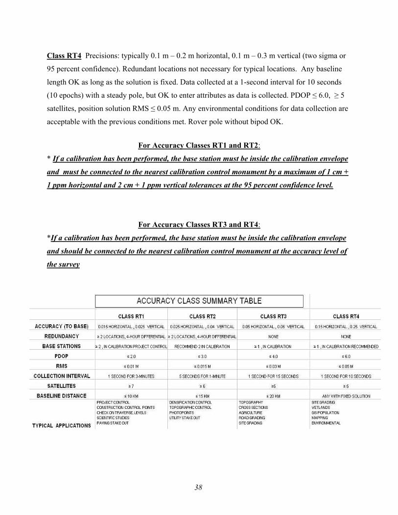
Note: Empirically, it has recently become evident that newer GNSS hardware and firmware using new algorithms might produce the various following accuracies over much longer baseline distances. Additionally, redundant positions at staggered times are showing a much closer numerical comparison than previously seen. This may mean that the Class RT1 accuracies could be obtained using the criteria for Class RT2, etc. Regardless of this, the user should at least be able to achieve the desired accuracy by using the appropriate criteria herein.

Class RT1 Precisions: typically 0.01 m – 0.02 m horizontal, 0.02 m – 0.04 m vertical (two

sigma or 95 percent confidence), two or more redundant locations with a staggered time interval

of 4-hours from different bases adjusted in the project control, each RT location differs from the

average no more than the accuracy requirement. Discard outliers and reobserve if necessary.

Base stations should use fixed height tripods. Baselines ≤ 10 KM (6 miles). Data collected at a 1-

second interval for 3 minutes (180 epochs), PDOP ≤ 2.0, ≥ 7 satellites, position solution RMS ≤

0.01 m. No multipath conditions observed. Rover range pole must be firmly set and leveled with

a shaded bubble before taking data. Use fixed height Rover pole with bipod or tripod for

stability.

Class RT2 Precisions: typically 0.02 m – 0.04 m horizontal, 0.03 m – 0.05 m vertical (two

sigma or 95 percent confidence), two or more redundant locations staggered at a 4-hour interval,

two different bases recommended, bases are within the project envelope, each location differs

from the average no more than the accuracy requirement. Discard outliers and reobserve if

necessary. Base stations should use fixed height tripods. Baselines ≤ 15 KM (9 miles) Data

collected at a 5-second interval for one minute (12 epochs). PDOP ≤ 3.0, ≥ 6 satellites, position

solution RMS ≤ 0.015 m. No multipath conditions observed. Rover range pole must be level

before taking data. Use fixed height Rover pole with bipod or tripod for stability.

Class RT3 Precisions: typically 0.04 m – 0.06 m horizontal, 0.04 m – 0.08 m vertical (two

sigma or 95 percent confidence). Redundant locations not necessary for typical locations,

important vertical features such as pipe inverts, structure inverts, bridge abutments, etc. should

have elevations obtained from leveling or total station locations, but RT horizontal locations are

acceptable. Baselines ≤ 20 KM (12 miles) Data collected at a 1-second interval for 15 seconds

(15 epochs) with a steady pole (enter attribute information before recording data). PDOP ≤ 4.0,

≥ 5 satellites, position solution RMS ≤ 0.03 m. Minimal multipath conditions. OK to use Rover

pole without bipod, try to keep pole steady and level during the location.

38

Class RT4 Precisions: typically 0.1 m – 0.2 m horizontal, 0.1 m – 0.3 m vertical (two sigma or

95 percent confidence). Redundant locations not necessary for typical locations. Any baseline

length OK as long as the solution is fixed. Data collected at a 1-second interval for 10 seconds

(10 epochs) with a steady pole, but OK to enter attributes as data is collected. PDOP ≤ 6.0, ≥ 5

satellites, position solution RMS ≤ 0.05 m. Any environmental conditions for data collection are

acceptable with the previous conditions met. Rover pole without bipod OK.

For Accuracy Classes RT1 and RT2:

* If a calibration has been performed, the base station must be inside the calibration envelope

and must be connected to the nearest calibration control monument by a maximum of 1 cm +

1 ppm horizontal and 2 cm + 1 ppm vertical tolerances at the 95 percent confidence level.

For Accuracy Classes RT3 and RT4:

*If a calibration has been performed, the base station must be inside the calibration envelope

and should be connected to the nearest calibration control monument at the accuracy level of

the survey

39

For Accuracy Classes requiring redundant locations, in addition to obtaining a redundant

location at a staggered time, use this procedure for each location to prevent blunders:

1. Move at least 30 m from the location to create different multipath conditions, invert the rover

pole antenna for 5 seconds, or temporarily disable all satellites in the data collector to force a

reinitialization, then relocate the point after reverting to the proper settings.

2. Manually check the two locations to verify that the coordinates are within the accuracy desired

or inverse between the locations in the data collector to view the closure between locations. Each

location should differ from the average by no more than the required accuracy.

3. Optionally, after losing initialization, use an “initialization on a known point” technique in the

data collector. If there was a gross error in the obtained location, initialization will not occur.

4. For vertical checks, change the antenna height by a decimeter or two and relocate the point.

(Don’t forget to change the rover’s pole height in the data collector!)

Quick Field Summary:

Set the base at a wide open site Set rover elevation mask between 12° & 15° The more satellites the better The lower the PDOP the better The more redundancy the better Beware multipath Beware long initialization times Beware antenna height blunders Survey with “fixed” solutions only Always check known points before, during and after new location sessions Keep equipment adjusted for highest accuracy Communication should be continuous while locating a point Precision displayed in the data collector is usually at the 68 percent level (or

1σ), which is only about half the error spread to get 95 percent confidence Have back up batteries & cables RT doesn’t like tree canopy or tall buildings

40

VI. Further Work in the Office RT baselines can be viewed and analyzed in most major GNSS software. The data is

imported into the software with the field parameters and project configuration intact. At this

point a recalibration can be done or the field calibration (if any) can be reviewed and left

unaltered.

* If the site calibration is changed in the office, resulting in new coordinates on all located

points, the new calibration information must be uploaded to the data collector before any

further field work is done for that project.

Communication between field and office is critical to coordinate integrity and consistency of

the project.

*If the data is collected with covariance matrices and there is redundancy or connecting

points, a post campaign adjustment can also be performed (although at less accuracy than

with static network observations).

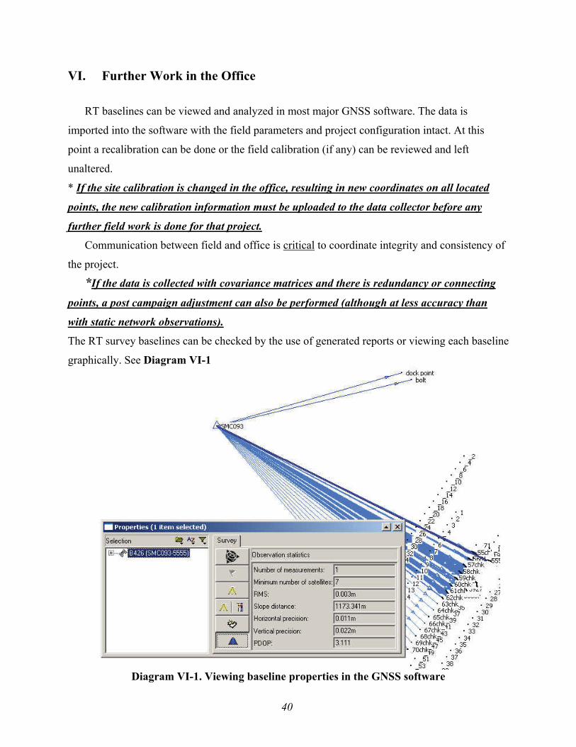
The RT survey baselines can be checked by the use of generated reports or viewing each baseline

graphically. See Diagram VI-1

Diagram VI-1. Viewing baseline properties in the GNSS software

41

* Entering in the correct coordinates of field checked stations will let the user actually adjust all the RT located points holding those known values.

(See “Appendix A” for a case field study by the Vermont Agency of Transportation under the

direction of NGS Geodetic Advisor Dan Martin)

Additional properties to office check in the RT data include:

• Antenna heights (height blunders are unacceptable and can even produce horizontal

error) (Meyer, et.al, 2005).

• Antenna types

• RMS values

• Redundant observations

• Horizontal & vertical precision

• PDOP

• Base station coordinates

• Number of satellites

• Calibration (if any) residuals

42

VII. Contrast to RTN Positioning

With the convergence of maturing technologies such as wireless Internet communication,

later generation GNSS hardware and firmware, and augmented satellite constellations, RT

positioning is becoming a preferred method of data acquisition, recovery and stake out to many

users in diverse fields. NGS is moving toward “active” monumentation via the CORS network

and its online positioning user service (OPUS). This is a departure from the traditional delivery

of precise geodetic control from passive monumentation. Currently, network solutions for RT

positioning are sweeping across the United States. The cost to benefit ratio and ease of use are

two main factors driving this rapid growth. As can be seen from the following list, the RTN

administrators span a wide sector of all GNSS users. Some examples of the RTN administrators

that are part of this rapidly expanding GNSS application are State Departments of Transportation

(DOT), Value Added GNSS Vendors, GNSS Manufacturers, Spatial Reference Centers,

Geodetic Surveys, Academic Institutions, Scientific Groups, County Governments, City

Governments, Private Survey/Engineering Companies and Agricultural Cooperatives

Benefits to the user of an RTN over classical RT positioning include:

1. No user base station is necessary. Therefore, there are no security issues with the base, no

control recovery is necessary to establish its position, and the user needs only half the equipment

to produce RT work. Additionally, there is no lost time setting up and breaking down the base

station equipment and radio.

2. The first order ppm error is eliminated (or drastically reduced) because ionospheric,

tropospheric and orbital errors are interpolated to the site of the rover.

3. The network can be positioned to be aligned with the NSRS with high accuracy. The users

will then be collecting positional data that will fit together seamlessly. This is important to all

users of geospatial data, such as GIS professionals who may deal with such regional issues as

emergency management and security issues.

4. Datum readjustments or changes can be done transparently to the user with no post campaign

work. New datum adjustments to NAD 83 or even transformations to another geodetic datum

such as the International Terrestrial Reference Frame (ITRF) are done at the network level and

are broadcast to the users.

5. With some business models, the user can share in the network profits by installing a network

reference station and getting a share of the subscription fees imposed upon other network users.

43

6. Different formats and accuracies are readily available. GIS data, environmental resource data,

mapping grade data, etc. can be collected with one or two foot accuracy while surveyors and

engineers can access the network with centimeter level accuracy. RTCM, CMR+ and other

binary formats can be user selected.

7. The RTN can be quality checked and monitored in relation to the NSRS using NGS programs

such as OPUS and TEQC from UNAVCO.

Drawbacks to the user of an RTN compared to classical RT positioning include:

1. Network subscription fees. These may be prohibitive for small companies.

2. Limited wireless data access.

3. Interpolation issues. Network spacing, communication and error modeling must be handled

optimally.

4. Work outside the network envelope (extrapolation of corrections) degrades accuracy.

5. The network solution may not fit to local control. Calibration may be necessary.

6. Coordinate metadata. Is the network datum the user’s required datum?

NGS has an important role to play in this new positioning solution, both in providing

support for these networks as well as protecting the public interest. In addition, NGS plans to

encourage RTN to successfully align to the NSRS within a certain tolerance (to be determined)

by connections to the CORS network. Following this document, NGS will develop user

guidelines and administrative guidelines for RTN in the effort to keep the produced positions

homogenous and accurate for all levels of geospatial professionals.

44

VIII. Classical Real Time Positioning Glossary Note: The definitions of the terms found below are adapted to fit the area of real time positioning and are not meant to be a rigorous, fully complete definition as found in the NGS Geodetic Glossary.

-A-

Autonomous Positioning

A single receiver position relative to a GNSS datum as realized by the satellites. No additional error modeling is done beyond broadcast models. A current civil user can expect better than 10 m accuracy under normal conditions autonomously.

Accuracy

The degree to which a particular RT point location measurement relates to the “truth”. In classical RT this is the defined by the horizontal and/or vertical positional error ellipse (or covariance matrix) at 95 percent (2σ) confidence level directly related to the base station as the representative of the datum. The base accuracy should always be known relative to the project datum.

Acquisition

The process of locking onto a satellite's available C/A and P code. A receiver acquires all available satellites when it is first powered up, then acquires additional satellites as they become available and continues tracking them until they become unavailable.

Algorithm

A special, logical method used to solve a certain type of mathematical problem. A set of programmed instructions to obtain an end result.

Almanac

A data file that contains the approximate orbit information of all satellites, which is transmitted by each satellite within its Navigation Message every 12.5 minutes (GPS). It is transmitted from the satellite to a receiver, where it facilitates rapid satellite signal acquisition within the receivers

45

by providing the receiver an approximate search area to acquire the satellite’s signals. Almanac data is kept current within a receiver to facilitate "hot starts" by permitting the Doppler Shift of each satellite signal to be determined and configuring each tracking channel for this Doppler-shifted carrier frequency. Doppler can detect cycle slips by tracking the path of the satellite relative to the receiver’s antenna.

Ambiguity / Ambiguity Resolution

Carrier phase measurements are made in relation to a cycle or wavelength of the L1 or L2 carrier waves. While the receiver can tag the partial cycle after locking on to a satellite, it can not directly know the whole number of cycles preceding that tag. This “ambiguity” of whole cycles must be solved in order to correctly calculate the distance from the satellite. The process or algorithm for determining the value for the ambiguities is “Ambiguity Resolution”. This can be done while the rover is moving which is known as “on the fly” AR (which requires dual frequency receiver capabilities). The number of cycles is different for each frequency to each satellite at each epoch. Once the ambiguity is removed using double differencing and other techniques, the initial count of the number of cycles can be maintained and differential positioning can be achieved by tracking the difference in cycles at the rover. Precisions by using the carrier phase can reach the millimeter level. Each sine wave length of the L1 frequency is 19.4 cm and that of the L2 is 24.2 cm. If there is signal obstruction or loss of communication, a "cycle slip" occurs, causing the new ambiguity after the cycle slip to be different from the value before. Cycle slip repair restores the continuity of carrier cycle counts and ensures that there is only one ambiguity for each satellite-receiver pair. Repair is aided through triple differencing and also Doppler tracking.

Antenna, GNSS

That part of the GNSS receiver hardware which receives and sometimes amplifies the incoming L-Band signals. Antennas vary in shape and size, but most these days use so-called "microstrip" or "patch" antenna elements. The base station should employ a ground plane antenna to help mitigate multipath. Fixed reference stations frequently use a "choke-ring" geodetic antenna to mitigate any multipath signals.

Antenna Phase Center

The electrical point, within or outside an antenna, at which the GNSS signal is measured. The realization of the phase center is determined by the set of antenna phase center variations (PCV) corrections that have been defined/adopted by NGS to account for the nonideal electrical response as a function of elevation and azimuth angles. The L1 and L2 phase centers are not identical. Traditionally, the NGS has modeled the phase center based on a relative variation from an antenna used as the reference. Current technology enables absolute phase center modeling to be performed rather than being relative to another antenna.

46

Antenna Reference Point

The point on the exterior of the antenna to which NGS references the antenna phase center position. It is usually the bottom of the antenna mount. Most RT firmware will use this height input to compute the actual modeled phase center using PCV models from the NGS or other sources.

Antenna Splitter

An attachment which can be used to split the antenna signal, so that it may be fed to two GNSS receivers. Such a configuration forms the basis of a Zero Baseline test.

Anti-Spoofing (AS)

Is a policy of the DoD by which the GPS P-Code is encrypted (by the additional modulation of a so-called W-Code to generate a new "Y-Code"), to protect the militarily important P-Code signals from being "spoofed" through the transmission of false GPS signals by an adversary during times of war. Hence civilian GPS receivers are unable to make direct P-Code pseudo-range measurements and must use proprietary (indirect) signal tracking techniques to make measurements on the L2 carrier wave (for both pseudo-range and carrier phase). All dual-frequency instrumentation must therefore overcome AS using these special signal tracking and measurement techniques. AS applies to the GPS constellation only.

47

Attribute

A characteristic which describes a feature (a point, line or polygon). Attributes are part of the data fields linked to the geospatial location of the Feature. Typically it is associated with geospatial data gathering for inclusion within Geographic Information Systems (GIS).

- B -

Baseline

A Baseline is a computed 3-D vector for a pair of stations for which simultaneous GPS data have been collected. It is mathematically expressed as a vector of Cartesian Earth Centered Earth Fixed (ECEF) X,Y,Z coordinate differences between the base or reference station and the rover or unknown station.

Base Station

Also called a Reference Station. In GNSS RT positioning, this is a receiver that is set up on a known location (at what ever accuracy) specifically to collect data for differentially correcting data files of the rover receiver. In the case of pseudo-range-based Differential GNSS (DGPS) the base station calculates the error for each satellite and, through differential correction, improves the accuracy of GNSS positions collected at the rover receiver. For GNSS RT Surveying techniques, the receiver data from the base station is combined with the data from the other receiver to form double-differenced observations, from which the baseline vector is determined.

Bias

All GNSS signals are affected by biases and errors. Biases are systematic errors that cause the observed measurements to be different from truth by a predictable or systematic amount, such as the lengthening of the signal path due to tropospheric refraction. Biases must somehow be accounted for in the data processing if high accuracy is sought. In classical RT positioning, many of the biases are treated as the same at the base station and the rover. Unmodeled biases such as multipath are outliers in the observables contributing to the position solution. One nanosecond of time delay is equivalent to 30 cm in range error.

Blunder

A gross error that prevents the desired position accuracy from being achieved. As opposed to systematic errors, such as a mal-adjusted circular vial level at the base station, or random errors

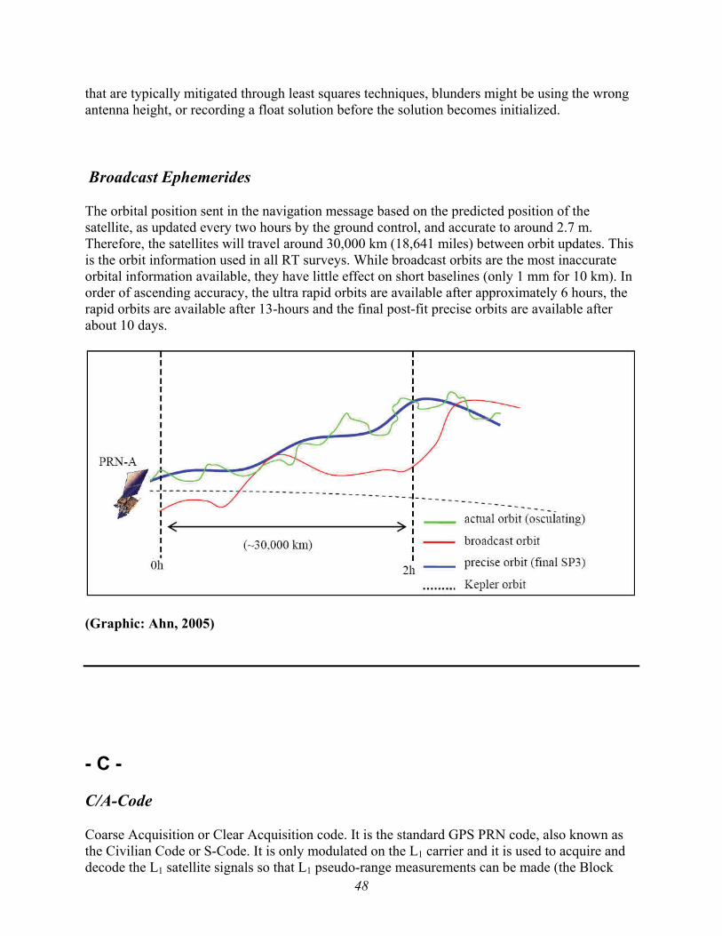
48

that are typically mitigated through least squares techniques, blunders might be using the wrong antenna height, or recording a float solution before the solution becomes initialized.

Broadcast Ephemerides

The orbital position sent in the navigation message based on the predicted position of the satellite, as updated every two hours by the ground control, and accurate to around 2.7 m. Therefore, the satellites will travel around 30,000 km (18,641 miles) between orbit updates. This is the orbit information used in all RT surveys. While broadcast orbits are the most inaccurate orbital information available, they have little effect on short baselines (only 1 mm for 10 km). In order of ascending accuracy, the ultra rapid orbits are available after approximately 6 hours, the rapid orbits are available after 13-hours and the final post-fit precise orbits are available after about 10 days.

(Graphic: Ahn, 2005)

- C -

C/A-Code

Coarse Acquisition or Clear Acquisition code. It is the standard GPS PRN code, also known as the Civilian Code or S-Code. It is only modulated on the L1 carrier and it is used to acquire and decode the L1 satellite signals so that L1 pseudo-range measurements can be made (the Block

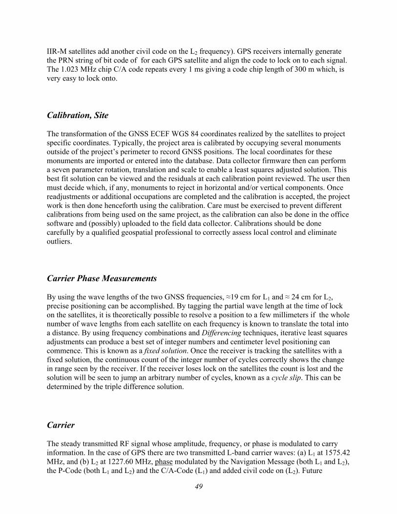
49

IIR-M satellites add another civil code on the L2 frequency). GPS receivers internally generate the PRN string of bit code of for each GPS satellite and align the code to lock on to each signal. The 1.023 MHz chip C/A code repeats every 1 ms giving a code chip length of 300 m which, is very easy to lock onto.

Calibration, Site

The transformation of the GNSS ECEF WGS 84 coordinates realized by the satellites to project specific coordinates. Typically, the project area is calibrated by occupying several monuments outside of the project’s perimeter to record GNSS positions. The local coordinates for these monuments are imported or entered into the database. Data collector firmware then can perform a seven parameter rotation, translation and scale to enable a least squares adjusted solution. This best fit solution can be viewed and the residuals at each calibration point reviewed. The user then must decide which, if any, monuments to reject in horizontal and/or vertical components. Once readjustments or additional occupations are completed and the calibration is accepted, the project work is then done henceforth using the calibration. Care must be exercised to prevent different calibrations from being used on the same project, as the calibration can also be done in the office software and (possibly) uploaded to the field data collector. Calibrations should be done carefully by a qualified geospatial professional to correctly assess local control and eliminate outliers.

Carrier Phase Measurements

By using the wave lengths of the two GNSS frequencies, ≈19 cm for L1 and ≈ 24 cm for L2, precise positioning can be accomplished. By tagging the partial wave length at the time of lock on the satellites, it is theoretically possible to resolve a position to a few millimeters if the whole number of wave lengths from each satellite on each frequency is known to translate the total into a distance. By using frequency combinations and Differencing techniques, iterative least squares adjustments can produce a best set of integer numbers and centimeter level positioning can commence. This is known as a fixed solution. Once the receiver is tracking the satellites with a fixed solution, the continuous count of the integer number of cycles correctly shows the change in range seen by the receiver. If the receiver loses lock on the satellites the count is lost and the solution will be seen to jump an arbitrary number of cycles, known as a cycle slip. This can be determined by the triple difference solution.

Carrier

The steady transmitted RF signal whose amplitude, frequency, or phase is modulated to carry information. In the case of GPS there are two transmitted L-band carrier waves: (a) L1 at 1575.42 MHz, and (b) L2 at 1227.60 MHz, phase modulated by the Navigation Message (both L1 and L2), the P-Code (both L1 and L2) and the C/A-Code (L1) and added civil code on (L2). Future

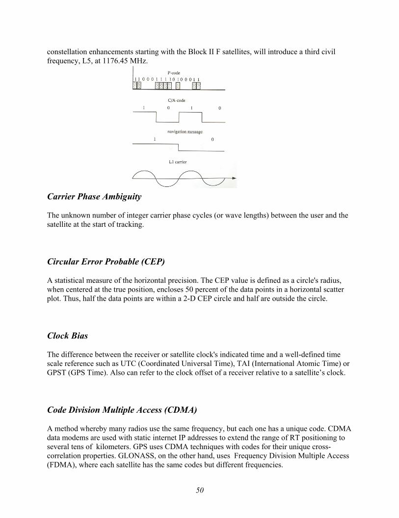
50

constellation enhancements starting with the Block II F satellites, will introduce a third civil frequency, L5, at 1176.45 MHz.

Carrier Phase Ambiguity

The unknown number of integer carrier phase cycles (or wave lengths) between the user and the satellite at the start of tracking.

Circular Error Probable (CEP)

A statistical measure of the horizontal precision. The CEP value is defined as a circle's radius, when centered at the true position, encloses 50 percent of the data points in a horizontal scatter plot. Thus, half the data points are within a 2-D CEP circle and half are outside the circle.

Clock Bias

The difference between the receiver or satellite clock's indicated time and a well-defined time scale reference such as UTC (Coordinated Universal Time), TAI (International Atomic Time) or GPST (GPS Time). Also can refer to the clock offset of a receiver relative to a satellite’s clock.

Code Division Multiple Access (CDMA)

A method whereby many radios use the same frequency, but each one has a unique code. CDMA data modems are used with static internet IP addresses to extend the range of RT positioning to several tens of kilometers. GPS uses CDMA techniques with codes for their unique cross-correlation properties. GLONASS, on the other hand, uses Frequency Division Multiple Access (FDMA), where each satellite has the same codes but different frequencies.

51

Code Phase

GPS measurements based on the C/A-Code. The term is sometimes restricted to the C/A- or P-Code pseudo-range measurement when expressed in units of cycles.

Constellation

Refers to either the specific set of satellites used in calculating a position, or all the satellites visible to a GNSS receiver at one time.

Control Point

Also called a control station or geodetic control station. A monumented point to which coordinates have been assigned by the use of terrestrial or satellite surveying techniques. The coordinates may be expressed in terms of a satellite reference coordinate system (such as WGS 84, or PZ 90), or a local geodetic datum. The official geodetic national horizontal datum for the United States is NAD 83 and the official vertical datum is NAVD 88.

Cut-off Angle

The minimum acceptable satellite elevation angle (above the horizon) to avoid the most noise in the GNSS signals due to atmospheric delay and refraction or possibly multipath conditions. Typically, cut off angles are set between 12˚ and 15˚ for RT surveying. Also called Elevation Mask.

Cycle Slip

A discontinuity of an integer number of cycles in the carrier phase count resulting from a loss of lock in the tracking loop of a GPS receiver. This corrupts the carrier phase measurement, causing the unknown Ambiguity value to be different after the cycle slip compared with its value before the slip. It requires a reinitialization of the receiver to repair the slip of the unknown number of "missing" cycles and the RT observations corrected by that amount.

Covariance (Matrix)

A measure of the correlation of errors between two observations or derived quantities. Also refers to an off-diagonal term in a variance-covariance matrix.

52

A covariance matrix is a matrix that defines the variance and covariance of an observation. The elements of the diagonal are the variance and all elements on either side of the diagonal are the covariance. Graphically, this matrix can define an error ellipse for the baseline or point position. ____________________________________________________________________

- D -

Data Collector

Also known as a data logger or data recorder. A handheld, relatively lightweight data entry computer, usually ruggedized. It stores the RT data collected in the field. In static GNSS surveying, the receiver is typically the repository for the data unless directed elsewhere. Also, it can be used to store additional data obtained by a GNSS receiver, such as Attribute information on a Feature whose coordinates are captured for a GIS project. Most collectors have coordinate geometry capability as well as the ability to perform calibrations, set elevation masks, block satellites, view satellite positions, change datums and units in the display. Modern data collectors are frequently touch screen capable and internet capable.

Datum (Geodetic)

Simply stated, a geodetic datum is defined by a reference surface, an origin, an orientation, gravity and a scale. For example, the NAD 83 datum is defined by the Geodetic Reference System 1980 (GRS 80) ellipsoid, at an origin near the center of the mass of the earth, with axes oriented through the pole, equator and at right angles, with a scale unit based on the international meter. The realization of the datum is through monumentation of some sort on, above or below the earth. The realization of WGS 84 is the GPS satellites themselves along with the ground control segment. We access WGS 84 through the satellites. All RT work is done in this datum and transformed by seven parameters (shifts X,Y,Z, rotations X,Y,Z and scale) to, for example, the displayed datum projection we view in the data collector. The elevations are obtained through a transformation from WGS 84 ellipsoid heights to NAD 83 ellipsoid heights where the geoid model can be applied to yield NAVD 88 orthometric heights. Alternatively, site calibrations create an inclined plane (that could be used with the geoid model as well) that is the result of the transformation of the RT WGS 84 positions to local control monumentation coordinates. (see Calibration).

Differential GPS (DGPS)

A code based technique to improve GPS accuracy (but not as accurately as carrier phase positioning) that uses computed pseudo-range errors measured at a known base station location to improve the measurements made by other GPS receivers within the same general geographic area. It may be implemented in RT through the provision of a communication link between the GPS receivers, transmitting the correction information in the industry-standard RTCM format, or

53

various proprietary formats. It may be implemented in single-base station mode, in the so-called Local Area DGPS (LADGPS), or using a network of base stations, as in the Wide Area DGPS (WADGPS) implementation.

Differential Positioning

Also known as relative positioning. Precise measurement of the relative positions of two receivers tracking the same GNSS signals. Usually associated with code based GPS positioning, but may be considered terminology for the more precise carrier phase-based baseline determination technique associated with GNSS Surveying.

Dilution of Precision (DOP)

An indicator of the effect of satellite geometry on positioning errors. Positions derived with a higher DOP value generally yield less accurate measurements than those derived with lower DOP. There are a variety of DOP indicators, such as GDOP (Geometric DOP), PDOP (Position DOP), HDOP (Horizontal DOP), VDOP (Vertical DOP), etc.

GDOP Uncertainty of all parameters (latitude, longitude, height, clock offset)

PDOP

Uncertainty of 3D parameters (latitude, longitude, height). This is the measure most frequently used as a guide in RT positioning. It is a unitless figure of merit expressing the relationship between the error in user position and the error in satellite position, which is a function of the configuration of satellites from which signals are derived in positioning. Geometrically, PDOP is proportional to 1 divided by the volume of the polyhedron formed by lines running from the receiver to the observed satellites. Small values, such as "2", are good for positioning while higher values produce less accurate position solutions. Small PDOP is associated with widely separated satellites. The UERE multiplied by the PDOP would give the expected, uncorrected position error.

HDOP

Uncertainty of 2D parameters (latitude, longitude)

VDOP

Uncertainty of height parameter

54

TDOP

Uncertainty of clock offset parameter

Doppler Shift

The apparent change in the frequency of a signal caused by the relative motion of the satellite and receiver. This can be used to detect cycle slips.

Double-Difference

A data processing procedure by which the pseudo-range or carrier phase measurements made simultaneously by two GNSS receivers are combined (differenced) so that, for any measurement epoch, the observations from one receiver to two satellites are subtracted from each other to remove that receiver's clock error (or bias) and hardware error. Two receivers to one satellite eliminate that satellite’s clock errors and hardware errors. The difference of these two single differences is then the double difference. It also significantly reduces the effect of unmodeled atmospheric biases and orbit errors. The resulting set of Double-Differenced observables (for all independent combinations of two-satellite-two-receiver combinations) can be processed to solve for the baseline (linking the two receivers) components and, in the case of ambiguous (unknown) carrier phase measurements, the integer ambiguity parameters. All high precision positioning techniques use some form of Double-Difference processing: pseudo-range, unambiguous carrier phase “fixed" solution (i.e., after the double-differenced ambiguity values have been estimated and applied to the original carrier measurements), or ambiguous carrier phase data within a "free" solution.

Dual-Frequency

Refers to the instrumentation that can make measurements on both GPS L-Band frequencies, or to the measurements themselves (e.g., L1 and L2 pseudo-range or carrier phase measurements). Dual-frequency measurements are useful for high precision RT because the Ionospheric Delay bias can be determined, and the data corrected for it. In the case of Double-Differenced carrier phase, dual-frequency observations can account for the residual ionospheric bias (for case of long baselines), and aid in Ambiguity Resolution. All "top-of-the-line" GPS receivers are of the dual-frequency variety, and are comparatively expensive because of the special signal processing techniques that must be implemented to make measurements on the L2 carrier under the policy of AS. RT positioning can be done with L1 only with limited range.

55

- E –

Earth-Centered, Earth-Fixed (ECEF) Coordinates

A reference to a (X, Y, Z) three-dimensional Cartesian coordinate frame attached to the Earth’s mantle, at certain epoch t, and the following definitions:

1. Origin: At the geocenter (Earth’s center of mass including atmosphere and oceans)

2. Z-axis: Directed toward the conventional definition of the North Pole, or more precise, towards the Conventional Terrestrial Pole (CTP) as defined by the International Earth Rotation Service (IERS). (Approximately coincides with the Mean Pole of rotation).

3. X-axis: Passes through the point of zero longitude (approximately on the Greenwhich meridian) as defined by the IERS.

4. Y-axis: Forms a right-handed coordinate system with the X- and Y-axes.

There are many realizations of this ideal ECEF frame frequently used by the geodetic-surveying community (e.g. ITRF97, ITRF2000, ITRF2005, WGS 84, etc.). The scale along the three Cartesian axes are given in linear units based on the modern definition of the international unit of length (the meter) = the distance traveled by light in a vacuum in 1/299,792,458 of a second.

The orbits of the GNSS satellite constellations are given in different ECEF frames and the user should be aware that the differences between them may be negligible or, to the contrary, appropriate transformations between frames must be implemented. This process is generally performed by the internal receiver software that gives the final results a pre-specified ECEF coordinate frame.

Z

Y X

Zero Meridian

Conventional Equatorial Plane

Orthogonal to “Z” axis

Geocenter

Conventional Terrestrial Pole

56

Elevation Mask

See Cut-Off Angle.

Ellipsoid Height (See Height, Ellipsoid)

Ephemeris (Ephemerides)

The file of values giving a particular satellite's position and velocity at any instant in time. The Broadcast Ephemeris for a satellite is the prediction of the current satellite position and velocity determined by the Master Control Station, uploaded by the Control Segment to the GPS satellites, and transmitted to the user receiver in the Data Message. The Precise Ephemerides are post-processed values derived by, for example, the International GNSS Service (IGS), and available to users post-mission via the Internet. Broadcast Ephemeris data is sufficient for short baseline RTK work, i.e. for baselines under 30 Km. Ephemeris errors are largely mitigated by double-differenced observables from carrier phase measurements when the receivers are up to a few tens of kilometers apart. Broadcast Ephemeris errors are typically around 2.7 m, while Precise Ephemeris errors are at the 1-2 cm level.

Epoch

A specific instant in time. RT GPS carrier phase measurements are made at a given interval (e.g. every 1 second) or epoch rate.

Error ellipse

A statistical measure of the positional error at a given point computed from the propagation of all errors contributing to the position, shown graphically in the GNSS software. Most modern GNSS receivers and data collector firmware can generate and save the position covariance matrix RT mode to import into software. Redundant and connected baselines can then be adjusted and error statistics generated. This is an excellent method to analyze the integrity of RTK results.

57

- F -

Federal Radionavigation Plan (FRP)

Congressionally mandated, joint DoD and US Department of Transportation (DoT) effort to reduce the proliferation and overlap of federally funded radionavigation systems. The FRP is designed to delineate policies and plans for US government-provided radionavigation services. Produced annually.

Fixed Ambiguity Estimates

Carrier phase ambiguity estimates which are set to a given number and held constant. Usually they are set to integers or values derived from linear combinations of integers. In an iterative, least squares process, the receiver performs algorithms to resolve the integer number of initial epoch wave lengths or cycles to each satellite on each frequency. The resolution of this ambiguity is necessary to perform differential carrier phase positioning. Once these are resolved, the ambiguities are said to be “fixed”.

Float Ambiguity

The estimated number of cycles and partial (decimal) cycles to each satellite on each frequency. The float ambiguity estimates are iterated through algorithms to produce a solution for the whole cycle count necessary to achieve centimeter level RT differential positioning. Float ambiguities are sometimes the only solution possible for long baselines (100+ km), but are considered adequate at those distances.

Frequency

The number of waves passing a specific point within a unit period of time, expressed in Hertz (cycles per second). E.g., the L1 frequency is 1.57542 million cycles per second or 1575.42 MHz.

Frequency Modulation (FM)

A method of encoding information in a carrier signal by altering the frequency while amplitude remains constant. The GPS carrier frequencies are modulated with the C/A code, P-code and navigation message.

58

- G – Galileo

The European Union’s satellite navigation system. Projected to be operational after 2010.

Geodetic Survey

Surveys for the establishment of control networks (comprised of active or passive Reference or Control Points), which are the basis for accurate positioning and navigation under, on or over the surface of the earth. May be carried out using either terrestrial or satellite positioning (e.g. GPS) techniques. “Geodetic” surveys imply that refraction, curvature of the earth, atmospheric conditions and gravity are taken into account in the measurements rather than “plane” surveys in which these factors are generally ignored. The outcome is a network of stations which are a physical realization of the Geodetic Datum or Reference System.

Geographic Information System (GIS)

A computer-based system that is capable of collecting, managing and analyzing geospatial data. It includes the networking systems, personnel, software, hardware and communication media to integrate the data. Generally speaking, it is a tabular database hot-linked to a graphical display of points, lines and polygons. Layers of data types of many different accuracies are represented separately or together. It has the ability to provide answers to data queries and can perform spatial analysis topologies from graphical and tabular data. RT techniques are frequently used with many facets of GIS, such as populating a utility infrastructure or locating photopoints for photogrammetric applications.

Geoid (Gravimetric), Geoid (Hybrid)

The equipotential surface (homogenous gravitational acceleration value) that most closely approximates global Mean Sea Level. Local mean sea level diverges from this surface due to factors such as constant winds, currents, salinity, etc. A conversion surface is applied to the Gravimetric Geoid (e.g., USGG 2003) to obtain the Hybrid Geoid Model (e.g., Geoid 03) which is used to convert the NAD 83 (our official national horizontal geodetic datum) ellipsoid heights from GNSS surveys into NAVD 88 (our official national vertical datum) orthometric heights.

59

Geoid Height

The separation distance between the ellipsoid (GRS 80) and the hybrid geoid model surface (e.g., Geoid 06). The combination of the NAD 83 ellipsoid height from GNSS observations and this value enables a NAVD 88 orthometric height to be produced. The geoid height is positive away from the earth center and negative towards it (it is below the ellipsoid across the CONUS). The RT user should have this model loaded into the data collector to be used whether a calibration is performed or not.

Geometric Dilution of Precision (GDOP)

See Dilution of Precision. An indicator of the geometrical strength of a GPS constellation used for a position/time solution (horizontal, vertical & time).

Global Navigation Satellite System (GNSS)

This is an umbrella term used to describe a generic satellite-based navigation/positioning system. It was coined by international agencies such as the International Civil Aviation Organization (ICAO) to refer to both GPS and GLONASS, as well as any augmentations to these systems, and to any future civilian developed satellite system. For example, the Europeans refer to GNSS-1 as being the combination of GPS and GLONASS, but GNSS-2 is the blueprint for an entirely new system. Future constellations may include China’s Compass, Europe’s Galileo, Japan’s QZSS, etc.

Global'naya Navigatsionnaya Sputnikovaya Sistema / Global Orbiting Navigation Satellite System (GLONASS)

This is the Russian Federation counterpart to GPS. It is designed to consist of a constellation of 24 satellites (though the number is presently less due to difficulties in funding for the system) transmitting on a variety of frequencies in the ranges from 1597-1617 MHz and 1240-1260 MHz (each satellite transmits on two different L1 and L2 frequencies). GLONASS provides worldwide coverage, however its accuracy performance is optimized for northern latitudes, where it is better than GPS's SPS. GLONASS positions are referred to a different datum than GPS, i.e. PZ90 rather than WGS84.

Global Positioning System (GPS)

A system for providing precise location which is based on data transmitted from a constellation of 30+ satellites. It comprises three segments: (a) the Control Segment, (b) the Space Segment,

60

and (c) the User Segment. The GPS constellation is a realization of the WGS 84 datum and is maintained by the Department of Defense. Users access the satellite specific codes and the L-band carrier signals to obtain positions using multilateration or for navigation.

GPS Surveying

Conventional static GPS surveying has the following characteristics: - The GNSS revceivers are all stationary. - GNSS data are collected in the receivers over an observation session, typically ranging in length from 20 minutes to several hours. - The results are obtained after post processing. - The positioning is obtained from relative positioning. - A variety of processing and error mitigation algorithms can be employed, including frequency combinations. - Mostly associated with the traditional surveying and mapping functions. - This method gives the highest accuracy and most reliability for GNSS positioning.

RT GPS surveying has the following characteristics: - One receiver is stationary for an entire campaign. One or more receivers are “rovers” that briefly visit points to be recovered or located. - GPS data are computed in the rover and displayed in the data collector in a few seconds or minutes. - The point of interest is obtained from relative positioning from the stationary receiver. - initialization is done “on the fly”. - Accuracy/precision is at the centimeter or two level which is sufficient for most surveying and engineering applications.

Additionally, GPS can be used for kinematic applications (navigation).

GPS Time (GPST)

GPST is a form of Atomic Time, as is, for example, Coordinated Universal Time (UTC). GPST is "steered" over the long run to keep within one microsecond of UTC. The major difference is that while "leap seconds" are inserted into the UTC time scale every 18 months or so to keep UTC approximately synchronized with the earth's rotational period (with respect to the sun), GPST has no leap seconds. At the integer second level, GPST matched UTC in 1980, but because of the leap seconds inserted since then, GPST is now ahead of UTC by 14 seconds (plus a fraction of a microsecond that varies from day to day). The relationship between GPST and UTC is transmitted within the Navigation Message.

61

Grid

A map coordinate system that projects the surface of the earth onto a flat surface such as a state plane or Universal Transverse Mercator (UTM) projection. Mapping grids have square zones for position measurements and can be based on strict Cartesian coordinates to maintain distances or more commonly, a conformal basis to maintain shapes.

Ground plane

A large flat metal surface, or electrically charged field, surrounding a GPS antenna used to shield the phase center from reflected signals.

- H -

Height (Ellipsoid)

Height above or below a mathematically defined ellipsoid (e.g., GRS 80 or WGS 84) that approximates the surface of the Earth. The height coordinate determined from GNSS observations is related to the surface of the WGS 84 reference ellipsoid. The WGS 84 ellipsoid height is natively displayed in RT GNSS positioning in a translation from the original computed ECEF X,Y,Z coordinates to latitude, longitude and ellipsoid height. However, data collection firmware can transform this into an orthometric height by use of the geoid model or by calibration to several known vertical bench marks.

Height (Orthometric)

The Orthometric Height is the height of a station on the earth's surface, measured as a distance curved along the local plumb line and normal to gravity from the reference surface to that station. The official US vertical datum is NAVD 88. Heights above or below that datum can be obtained through GNSS methods by using the current hybrid geoid model and the ellipsoid heights.

H = C / g = True Orthometric Height.

g is the average gravity along the plumb line which is impossible to know. Therefore, we use Helmert heights which approximate the average gravity by using surface gravity (g) and a constant value. C is the geopotential number which is a unitless value of the difference in gravitational acceleration or potential between two equipotential surfaces.

H = C / (g + 0.0424 H0) = Helmert Orthometric Height

62

Hertz

A unit used to measure a wave's frequency, one cycle per second. The three GPS frequencies are 1575.42 MHz, 1227.60 MHz and 1176.45 MHz (future). GLONASS uses unique frequencies in the L band for each satellite.

- I -

I/O

Abbreviation for Input/Output.

Ionosphere, Ionospheric Delay

The Ionosphere is that band of atmosphere extending from about 50 to 1000 km above the earth in which the sun's radiation frees electrons from the gas molecules (typically oxygen and nitrogen) present creating ions. The free electrons affect the speed and direction of the GNSS signals. The Ionospheric group delay is frequency-dependent (“dispersive”) and inversely proportional to the frequency. Therefore, the higher the frequency, the less is the ionospheric effect. A linear combination of the two GPS frequencies can substantially eliminate first order iono delay errors. The magnitude of the Ionospheric Delay is a function of the latitude of the receiver, the season, the time of day, and the level of solar activity. RT positioning assumes identical ionospheric conditions for base and rover and thus the error terms are neglected. The residual errors are baseline distance correlated, typically combined with the tropospheric error residuals and orbital errors into a 1-PPM error factor.

Ionosphere-Free Combination

A linear combination of the GPS L1 and L2 carrier phase measurements which provides an estimate of the carrier phase observation on one frequency with the effects of the ionosphere removed. It provides a different ambiguity value (non-integer) than a simple measurement on that frequency. However, there still remain unmodeled ionospheric errors of between 1 – 3 cm due to conditions such as the bending of the signal.

63

The ionosphere-free L1 carrier phase combination (in units of L1 wavelengths) is: f(L1)ion-free = a1.f(L1) + a2.f(L2)

with a1 = f12 /( f12 - f22 ) and a2 = - f1 . f2 / (f12 - f22) , f1 and f2 are the frequencies of the L1 and L2 carrier waves respectively. (A similar expression can be developed for the ionosphere-free L2 carrier phase.) The ionosphere-free pseudo-range combination (in metric units) is: Pion-free = b1.P(L1) + b2.P(L2) Iono-Free Carrier Phase Observation with

b1 = f12 / (f12 - f22) and b2 = - f22/ (f12 - f22) .

International Global Navigation Satellite System Service (IGS)

An initiative of the International Association of Geodesy, as well as several other scientific organizations, that was established as a service at the beginning of 1994. The IGS comprises of many component civilian agencies working cooperatively to operate a permanent global GNSS tracking network, to analyze the recorded data and to disseminate the results to users via the Internet. The range of "products" of the IGS include precise post-mission GPS satellite ephemerides, tracking station coordinates, earth orientation parameters, satellite clock corrections, tropospheric and ionospheric models. Although these were originally intended for the geodetic community as an aid to carrying out precise surveys for monitoring crustal motion, the range of users has since expanded dramatically, and the utility of the IGS is such that it is vital to the definition and maintenance of the International Terrestrial Reference System (and its various "frame realizations" ( ITRF96,ITRF2000, ITRF2005 etc.).

International Terrestrial Reference System (ITRS)

The most precise, geocentric, globally-defined coordinate system or datum of the earth. It is a more accurate than the WGS84 Datum. The various "frames" (such as ITRF2000, etc.) are realizations of the ITRS for a particular epoch in time, consisting of a set of 3-D coordinates and velocities for hundreds of geodetic stations around the world (all coordinates of fixed stations on the earth change with time due to plate tectonics). Although some of the stations are Satellite Laser Ranging (SLR) stations, or Very Long Baseline Interferometry (VLBI) stations, the vast majority are GNSS tracking stations of the IGS network. The ITRS is managed by the International Earth Rotation and Reference System Service (IERS) – a scientific organization with a Central Bureau in Frankfurt, Germany.

64

- J -

- K – Kalman Filter

An iterative mathematical procedure for estimating dynamically changing positions, such as the position and/or velocity of a rover, from observations. The a priori dynamic condition is usually input – walking, car, plane, etc. to help the program develop appropriate weighting and to remove outliers from its solution sets.

Kinematic Positioning

The user's GPS antenna is moving. In GPS, this term is typically used with precise carrier phase positioning, and the term “differential or dynamic positioning” is used with pseudorange positioning. Applications of Kinematic RT positioning include topography across open terrain, road profiling and shoreline locations. It can produce a line or a series of points by setting the observation parameters to automatically log locations at user selected distance and/or time intervals.

- L -

L1 Frequency

The 1575.42MHz GPS carrier frequency which contains the C/A-Code, the encrypted P-Code (or Y-Code) and the Navigation Message. Commercial GPS navigation receivers can track only the L1 carrier to make pseudo-range (and sometime carrier phase and Doppler frequency) measurements, while the P code can only be accessed for military applications.

L2 Frequency

The 1227.60MHz GPS carrier frequency which contains only the encrypted P-Code (or Y-Code) and the Navigation Message. Military Y-Code capable receivers can, in addition to making L1 measurements, make pseudo-range measurements on the L2 carrier. The combination of the two measurements (on L1 and L2) permits the Ionospheric Delay to be corrected for, since the ionosphere affects the different frequencies inversely to the square of their frequency. Dual-frequency GPS receivers intended for surveying applications can make L2 measurements using proprietary signal processing techniques. Such measurements are essential if the Ionospheric Delay on carrier phase is to be corrected (especially on baselines of length greater than about 20-

65

30km) and/or where fast Ambiguity Resolution is needed. Other combinations include wide lane (L1 – L2) and narrow lane (L1 + L2).

L-Band

The group of radio frequencies extending from 390MHz to 1550MHz. The GPS carrier frequencies L1 and L2 are in the L-Band.

Latency

The age or time lapse in corrections used in RT GPS. The longer the time lapse between the corrections, the less accurate they become at the rover.

- M -

Multipath

Interference caused by reflected GPS signals arriving at the receiver, typically as a result of nearby structures or other reflective surfaces. The reflected signal is delayed causing an apparent longer distance to the satellite. May be mitigated to some extent through appropriate antenna design, antenna placement and special filtering algorithms within GPS receivers in static observations, but not for the brief time on point for RT positioning. Usually the noise effect on RT positioning is a few centimeters unless it causes an incorrect ambiguity resolution, which might result in decimeters of error.

- N – NAD 83 The North American Datum of 1983. The official national horizontal datum for the United States as stated in the Federal Register / Vol. 60, No. 157, Docket No. 950728196--5196-011. NAD 83 is a three dimensional datum with the coordinates of points usually expressed in latitude, longitude and ellipsoid height. The current realization, NAD 83(CORS 96), is defined in terms of a 14 parameter Helmert transformation from the International Terrestrial Reference Frame of 1996. The NAD 83 origin located near the center of mass of the earth is biased relative to that of the ITRF by about 2.24 meters.

66

Narrow Lane Observable

The GPS observable obtained by summing the carrier-phase observations of a single epoch measured in cycles, on the L1 and L2 frequencies. That is L1 + L2.The effective wavelength of the narrow-lane observable is 10.7 centimeters. The narrow-lane observable can help resolve carrier-phase ambiguities.

Navigation Message

Contains the satellite's broadcast ephemeris, satellite clock bias correction parameters, constellation almanac information and satellite health. A 1500 bit message modulated on the L1 and L2 GPS signal broadcast approximately every 12.5 minutes.

NAVD 88

The North American Vertical Datum of 1988.

NAVSTAR

The GPS satellite system of the DoD. NAVSTAR is an acronym for “NAVigation Satellite Timing and Ranging”.

NMEA

National Marine Electronics Association, a U.S. standards body that defines message structure, content and protocols to allow electronic equipment installed within ships and boats to communicate with each other. GPS receivers can be configured to output various types of messages in the "NMEA format". The NMEA GSV message type should contain signal to noise ratio information and the GGA message contains the raw position..

Noise

An interfering signal that tends to mask the desired signal at the receiver output and which can be caused by space and atmospheric phenomena, can be human made, or can be caused by receiver circuitry. Also called White Noise.

67

- O -

OEM

Original Equipment Manufacturer. Typically GPS receiver "boardsets", “chip sets” or "engines" that a product developer can embed within some application or hardware package.

On-The-Fly (OTF)

This is a form of Ambiguity Resolution (AR) which does not require that the rover receiver remain stationary for any length of time. Hence this AR technique is suitable for initializing RTK Positioning. For many applications this introduces considerable flexibility. If a loss of lock occurs, the rover can reinitialize wherever it is located without revisiting a known point.

Oscillator

A device that generates a signal of a given frequency within the receiver.

Outage

Defined as a loss of availability of positional display data and computation, due to either there not being enough satellites visible to calculate a position (at least 5 are needed), or the value of the PDOP indicator is greater than some user specified value which prevents locations from being taken.

- P -

P-Code

The Precise or Protected code. A pseudorandom string of bits that is used by GPS receivers to determine the range to the transmitting GPS satellite on the GPS L1 and L2 carrier at a chip rate of 10.23MHz (approximately 10 times the resolution of the C/A code), which repeats about every 267 days. Each one-week segment of this code is unique to a GPS satellite and is reset each week. Under the policy of the DoD, the P-code is replaced by an encrypted Y-code when Anti-Spoofing is active. Y-code is intended to be available only to authorized (primarily military) users.

68

Phase Center

The apparent center of signal reception at an antenna. The electrical phase center of an antenna is not constant but is dependent upon the observation angle and azimuth to the satellite. The L1 and L2 phase centers are at different locations.

Position

The 3-D coordinates of a point, usually given in the form of latitude, longitude, and ellipsoidal height, though it may be provided in the 3-D Cartesian form (ECEF X,Y,Z), or any other transformed map or geodetic reference system. An estimate of error is often associated with a position.

Position Dilution of Precision (PDOP)

See Dilution of Precision. Measure of the geometrical strength of the GPS satellite configuration for 3-D positioning.

Post-Processed GNSS

In post-processed GNSS the base and user (or roving or mobile) receivers have no data communication link between them. Instead, each receiver records the satellite observations that will allow the processing of double-differenced observables (in the case of carrier phase-based positioning) at a later time. Data processing software is used to combine and process the data collected from these receivers.

Precise Positioning Service (PPS)

The most accurate absolute positioning possible with GPS navigation receivers, based on the dual-frequency encrypted P-Code. Available to the military users of GPS. Typical accuracy is of the order of 30 cm.

Precision

The degree of repeatability that measurements of the same quantity display, and is therefore a means of describing the quality of the data with respect to random errors. Precision is traditionally measured using the standard deviation and therefore is shown in the RMS error on the data collector screen. It can be thought of as the parameters of the positional error.

69

Pseudo-Random Noise (PRN )Number

A number assigned by the GPS system designers to a given set of binary signals with random noise-like properties. It is generated by mathematical algorithm or "code", consisting of a repeated pattern of 1's and 0's. The C/A-Code and the P-Code are examples of PRN codes. Each GPS satellite transmits a unique C/A-Code and P-Code sequence (on the same L1 and L2 frequencies), and hence a satellite may be identified according to its "PRN number", e.g. PRN2 or PRN14 are particular GPS satellites.

Pseudo-Range

A distance measurement based on the alignment of a satellite's time tagged transmitted code (may be the C/A-Code or the encrypted P-Code) and the local receiver's generated reference code (for that PRN satellite number), that has not been corrected for clock bias. Hence a pseudo-range measurement is a distance measurement biased by a time error. The C/A-Code pseudo-range measurements may have a spread of meters. The pseudorange is obtained by multiplying the apparent difference in time by “c” (the speed of light).

- R -

Range

The distance between two points, such as between a satellite and a GNSS receiver. Can be called Topocentric or Geometric range.

Real-time Kinematic (RTK or RT)

The relative positioning procedure whereby carrier phase observables and corrections for each L1 and L2 signal to each common satellite are transmitted in RT from a reference or base station to the user's rover receiver. The rover receiver processes the data in RT. Centimeter level accuracy is achieved without any post processing.

70

Reference Station

A ground station at a known location used to derive differential corrections. The reference station receiver tracks all satellites in view, corrects pseudorange errors, and then transmits the corrections with the carrier phase observables to the rover. Since all positions calculated are from vectors relative to the reference station, an autonomous position can be used in the field. When the true position is entered into the project, either in the field or office, all rover positions are updated to be relative to that position. Also called a base station.

Relative Positioning

The determination of relative positions between two or more receivers which are simultaneously tracking the same GNSS signals. One receiver is generally referred to as the reference or base station, whose coordinates are usually known in the project datum. The second receiver (rover) moves to various points to be recovered or located. Its coordinates are determined relative to the base station. In carrier phase-based positioning this results from the determination of the delta X,Y,Z coordinates applied as a baseline vector, which is added to the base station’s coordinates to generate the rover's coordinates.

Relative Precision

Precision is defined as a measure of the spread of a set of numbers around a number determined by the set (e.g. the mean). This is typically shown in a normal distribution as the standard deviation (σ) with respect to the mean. This is reflected in the data collector screen as the RMS. Relative precision shows the range of the components (X, Y, Z or N, E, up) between one station and other.

Root Mean Square (RMS)

Mathematically, it is the square root of the average of the sum of the squared residuals from the computed value. The RMS error approximates the 68 percent confidence level. Double the value to get the approximate 95 percent confidence level of the RT position. It is not related to satellite geometry, but rather is a geometry-free position solution spread of results.

Rover

Any mobile GPS receiver collecting data during a field session. The receiver's position is computed in the rover receiver relative to a stationary GNSS receiver at a base station.

71

Radio Technical Commission for Maritime Services (RTCM)

RTCM Special Committee 104 develops standard message types for use in differential GNSS positioning. The message content has been defined and hence when the RTCM-104 standard (version 3.1 is the latest) is implemented within a user receiver, it is able to decode and apply the differential corrections to its raw data in order to generate an error corrected coordinate.

- S -

Satellite Constellation

The orbiting satellites and their broadcast signals. The GNSS refers to the entire array of available satellites. GPS, GLONASS, Galileo and Compass are some individual constellations that can be used for positioning, navigation and timing – either collectively as they become available or individually.

Selective Availability (S/A)

Intentional degradation of the autonomous position capability of the GPS for civilian use by the U.S. military. This is accomplished by artificially "dithering" the clock error in the satellites. S/A was activated on 25 March 1990, and was “turned down” on the 1st May 2000 (midnight Washington D.C. time).

Signal to Noise Ratio (SNR, S/N, C/N0)

The ratio of incoming signal strength to the amount of interfering noise as measured in decibels on a logarithmic scale. Measurements have reliability if the SNR is 30 or greater.

Single Difference A GPS observable formed by arithmetically differencing carrier phases that are simultaneously measured by a pair of receivers tracking the same satellite, or by a single receiver tracking a pair of satellites. The between-receiver's single difference procedure removes all satellite clock and

72

hardware errors or conversely, the between-satellite’s single difference procedure removes the receiver’s clock and hardware errors. (see Appendix B)

Spatial Decorrelation

The increase in positional errors due to the increase in distance between the user and the reference station. When calculating differential corrections, the greater the distance between the two, the greater the error residual in the corrections. Errors that are thus correlated are commonly expressed in parts per million (PPM). These are primarily dispersive (frequency dependent) as in the ionospheric advance and refractive delay, and non-dispersive (geometrical) as in the tropospheric delay and refraction and in the orbital errors.

Standard Positioning Service (SPS)

The civilian absolute positioning accuracy obtained by using the pseudo-range data obtained with the aid of a standard single or dual frequency C/A-Code GPS receiver. Autonomous positioning currently yields around 10 m accuracy with SA turned down.

- T –

TDOP Time Dilution of Precision. See DOP

Triple-Difference

A linear combination of double-difference carrier phase observables by which the cycle ambiguity parameters can be eliminated and which is less affected by unrepaired cycle slips than double-differences. A triple-differenced observable is created by differencing two consecutive double-differences (the same pair of receivers and the same pair of satellites, but separated in time). A useful observable for obtaining approximate baseline solutions or for detecting cycle slips in the double-differenced observables.

73

Troposphere, Tropospheric Delay

The Troposphere is the neutral atmosphere from the earth’s surface to around 50 km altitude. The Tropospheric Delay on GPS signals is of the non-dispersive variety because it is not frequency-dependent and hence impacts on both the L1 and L2 signals by the same amount (unlike that within the Ionosphere). The wet and dry components of the Troposphere cause the signal refraction and delay, with the wet component be responsible for approximately 10 percent of the total delay, but being hard to model correctly. The dry or hydrostatic component is more easily modeled. Various Tropospheric models (Saastamoinen, Modified Hopfield, etc.) have been developed to estimate the delay as a function of the satellite elevation angle, receiver height, and “weather” components such as temperature, pressure and humidity. Zenith total delay (ZTD) is between 2 and 3 meters, but increases as the satellite is closer to the horizon to a factor of 5. RT processing essentially ignores differences in tropospheric conditions between the rover and base and therefore residual errors increase with baseline length. RT should not be performed with adverse or differing tropospheric conditions – such as when a weather front is passing through the project.

Time-To-First-Fix (TTFF)

The actual time required by a GPS receiver to achieve a position solution. The time will vary with site conditions, receiver type and whether the rover has carried any satellites from a previous loss of lock.

- U - Ultra High Frequency (UHF)

Radio frequencies in the band from 300 MHz to 3,000 MHz

User Equivalent Range Error (UERE)

Any error contributing to the error budget of autonomous GPS receiver positioning, expressed as an equivalent error in the range between a user's antenna and a satellite. UERE errors originate from different sources and thus are independent of each other. The total UERE is the square root of the sum of the squares of the individual errors. A prediction of maximum anticipated total UERE (minus ionospheric error) is provided in each satellite's navigation message as the user range accuracy (URA).

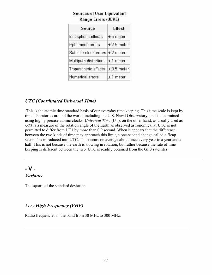
74

UTC (Coordinated Universal Time)

This is the atomic time standard basis of our everyday time keeping. This time scale is kept by time laboratories around the world, including the U.S. Naval Observatory, and is determined using highly precise atomic clocks. Universal Time (UT), on the other hand, as usually used as UT1 is a measure of the rotation angle of the Earth as observed astronomically. UTC is not permitted to differ from UT1 by more than 0.9 second. When it appears that the difference between the two kinds of time may approach this limit, a one-second change called a "leap second" is introduced into UTC. This occurs on average about once every year to a year and a half. This is not because the earth is slowing in rotation, but rather because the rate of time keeping is different between the two. UTC is readily obtained from the GPS satellites.

- V - Variance

The square of the standard deviation

Very High Frequency (VHF)

Radio frequencies in the band from 30 MHz to 300 MHz.

75

- W – Wide-Lane Observable The GPS observable obtained by differencing the carrier-phase observations of a single epoch measured, in cycles, on the L1 and L2 frequencies. That is, L1 – L2. The effective wavelength is 86.2 centimeters. It can be useful in resolving carrier-phase ambiguities.

World Geodetic System 1984 (WGS84)

A global geodetic datum defined and maintained by the DoD. As the control segment coordinates and the broadcast ephemerides are expressed in this datum, the GNSS positioning results are said to be in the WGS84 datum. Autonomously , WGS 84 differs from NAD 83 by over a meter. Augmentation of the constellations will enable users to see this difference with handheld units in the near future. The WGS84, PZ 90 and the ITRS are compatible at the few centimeters level. However, the ITRS is a more precise realization of an ECEF terrestrial reference system as shown in the iterations of the ITRF.

76

References

1) Ahn, Yong Won (M.Sc. thesis), (2005), Analysis of NGS CORS Network for GPS RTK Performance Using External NOAA Tropospheric Corrections Integrated with a Multiple Reference Station Approach, UCGE Report 20211.

2) Beutler, G., Bauersima, I., Gurtner, W., Rothacher, M., Schildknecht, T. & Geiger, A., (1989). Atmospheric refraction and other important biases in GPS carrier phase observations. In monograph 12, Atmospheric Effects on Geodetic Space Measurements, F.K.Brunner (ed.), School of Geomatic Engineering (formerly Surveying), The University of New South Wales, 15-44.

3) Caltrans/Division of Right of Way and Land Surveys, Surveys Manual, (2006).webpage http://www.dot.ca.gov/hq/row/landsurveys/SurveysManual/Manual_TOC.html

4) Caroline Erickson (M.Sc. thesis),(1992), Investigations of C/A Code and Carrier Measurements and Techniques for Rapid Static GPS Surveys, UCGE Report No. 20044. http://www.geomatics.ucalgary.ca/Papers/Thesis/GL/92.20044

5) Dao, Thi Hong Diep, (2005). Performance Evaluation of Multiple Reference Station GPS RTK for a Medium Scale Network. UCGE Report 20214. http://www.geomatics.ucalgary.ca/links/GradTheses.html

6) Gutman, S., T. Fuller-Rowell and D. Robinson (2003). Using NOAA Atmospheric Models to Improve Ionospheric and Tropospheric Corrections, U.S. Coast Guard Differential GPS Symposium, June 2003, Portsmouth, USA http://www.gpsmet.noaa.gov/jsp/downloads/NOAA_Atmospheric_Corrections.ppt.

7) International Organization for Standardization (ISO) TC 172/SC 6 (2008).Optics And Optical Instruments- Field Procedures For Testing Geodetic And Surveying Instruments - Part 8: GNSS Field Measurement Systems In Real-Time Kinematic (RTK), http://www.iso.org/iso/iso_catalogue/catalogue_tc/catalogue_detail.htm?csnumber=42213

8) Landau, H. and Euler, H. J., (1992), On-The-Fly Ambiguity Resolution for Precise Differential Positioning, ION GPS-92 Proceedings, Albuquerque, New Mexico, pp. 607-613.

9) Langley, R.B., (1997), GPS Receiver System Noise, GPS World, Vol. 8, No. 6, pp.40-45 G_____ ______ 344:_ *_____ _C_ _________ __________ 5_ 8_____ 10) Leick, A., (2004), Wiley, GPS Satellite Surveying, 3rd Edition 11) Mader, G. (1990): Ambiguity Function Techniques for GPS Phase Initialization and

Kinematic Solutions. Proceedings of the Second International Symposium on Precise Positioning with the Global Positioning System, Ottawa, Canada, Sept. 1990.

12) Meyer, T.H., Bean, J.E., Ferguson, C.R. & Naismith, J.M. (2002), The Effect of Broadleaf Canopies on Survey-Grade Horizontal GPS/GLONASS Measurements, Surveying and Land Information Science 62(4), 215–224.

13) Meyer, T. H., Hiscox, A.(2005), Position Errors Caused By GPS Height of Instrument Blunders, webpage http://digitalcommons.uconn.edu/thmeyer_articles/4/

14) New York State Department of Transportation/Land Surveying section, (2005), Land Surveying Standards and Procedures Manual. webpage https://www.nysdot.gov/portal/page/portal/divisions/engineering/design/design-services/land-survey/standards-procedures

15) NOAA (2005) Space Weather Prediction Center. webpage. http://www.sec.noaa.gov

15) Remondi, B. W., (1984), Using the Global Positioning System (GPS) phase observable for relative geodesy: modeling, processing, and results, PhD Thesis, University of Texas at Austin.

77

16) Remondi, B. W., Performing Centimeter-Level Surveys in Seconds with GPS Carrier Phase: Initial Results, Journal of The Institute of Navigation, Vol. 32, No. 4, Winter 1985-6

17) Yang X., Brock R., RDOP Surface for GPS Relative Positioning, United States Patent 6057800, issued May 2, 2000, web page http://www.patentstorm.us/patents/6057800-fulltext.html

18) Zilkoski, D.; D'onofrio, J.; Frakes, S. (1997). NOAA Technical Memorandum NOS-NGS-58 Guidelines for Establishing GPS-Derived Ellipsoid Heights (Standards: 2 cm and 5 cm) Version 4.3, November 1997, webpage http://www.ngs.noaa.gov/PUBS_LIB/NGS-58.html 19) Zilkoski, D.; Carlson, E.; Smith, C., (2005). Draft Guidelines for Establishing GPS-Derived

Orthometric Heights (Standards: 2 cm and 5 cm) Version 1.4. webpage http://www.ngs.noaa.gov/PUBS_LIB/pub_index.html

APPENDIX A AbstractReal Time Kinematic (RTK) surveying has been in use now for over a decade. However, there

is minimal documentation available relative to suggested field procedures designed to produce

positions of specific accuracies. Additionally, the methods for transmitting and receiving RTK

corrections have expanded to include the use of cellular modems, thus overcoming the distance

dependency of traditional UHF radio broadcasts and most manufactures support the collection

and processing of Global Navigation Satellite Systems (GNSS) such as GLONASS. The below

describes a case study into the use of single base RTK GNSS corrections being generated by the

VT CORS Network and accessed with a cellular modem. The Vermont CORS Network is

briefly described. Occupation time, baseline length, and field procedures are discussed and

compared. The results of this case study indicate that the guidelines listed for RT1, RT2, RT3,

and RT4 will in fact produce the stated accuracies.

Introduction

In the fall of 2006, the Vermont Agency of

Transportation began an ambitious effort to

establish a state-wide network of

Continuously Operating GNSS Reference

Stations (CORS). This CORS infrastructure

would be designed to provide both archived

data for post-processing as well as real-time

corrections (single baseline) to support Real

Time Kinematic (RTK) surveys. By the

spring of 2007 the first eleven stations were

in place and available for real-time

applications. The Vermont CORS network

is being designed to have a station spacing

of approximately 40km to 50km. (See figure

1)

The GNSS antenna’s for the CORS were

positioned relative to NAD83

CORS96(Epoch 2002) by submitting

numerous 12-hour datasets to the NGS’

Online User Positioning Service (OPUS).

The OPUS solutions for each station were

combined and then averaged to establish the

position of the GNSS Antenna Reference

Point (ARP).

Field Testing Procedure

Stations to be occupied

RTK observations were taken on existing

control stations that are part of the National

Spatial Reference System

Figure 1 - Current configuration of VT CORS

Network

(NSRS). The published coordinates from

the new national readjustment (NAD83

NSRS2007) would be used as truth.

Whenever possible, stations that also had a

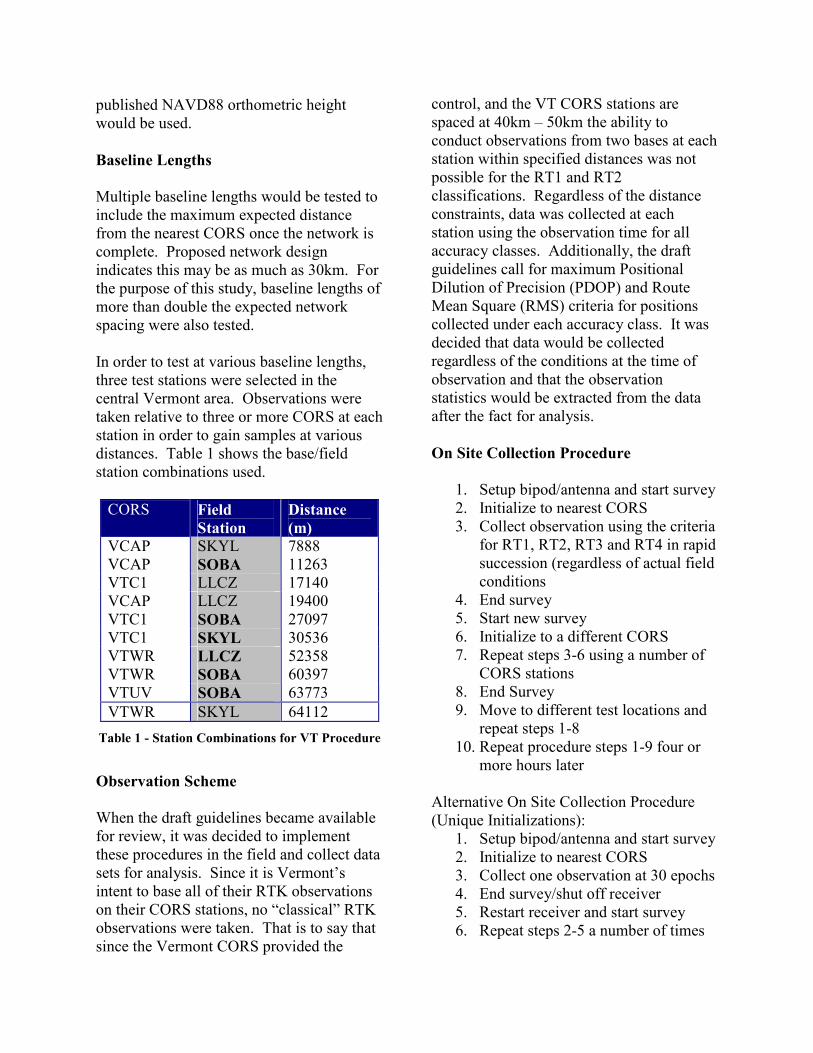
published NAVD88 orthometric height

would be used.

Baseline Lengths

Multiple baseline lengths would be tested to

include the maximum expected distance

from the nearest CORS once the network is

complete. Proposed network design

indicates this may be as much as 30km. For

the purpose of this study, baseline lengths of

more than double the expected network

spacing were also tested.

In order to test at various baseline lengths,

three test stations were selected in the

central Vermont area. Observations were

taken relative to three or more CORS at each

station in order to gain samples at various

distances. Table 1 shows the base/field

station combinations used.

CORS Field

Station

Distance

(m)

VCAP SKYL 7888

VCAP SOBA 11263

VTC1 LLCZ 17140

VCAP LLCZ 19400

VTC1 SOBA 27097

VTC1 SKYL 30536

VTWR LLCZ 52358

VTWR SOBA 60397

VTUV SOBA 63773

VTWR SKYL 64112

Table 1 - Station Combinations for VT Procedure

Observation Scheme

When the draft guidelines became available

for review, it was decided to implement

these procedures in the field and collect data

sets for analysis. Since it is Vermont’s

intent to base all of their RTK observations

on their CORS stations, no “classical” RTK

observations were taken. That is to say that

since the Vermont CORS provided the

control, and the VT CORS stations are

spaced at 40km – 50km the ability to

conduct observations from two bases at each

station within specified distances was not

possible for the RT1 and RT2

classifications. Regardless of the distance

constraints, data was collected at each

station using the observation time for all

accuracy classes. Additionally, the draft

guidelines call for maximum Positional

Dilution of Precision (PDOP) and Route

Mean Square (RMS) criteria for positions

collected under each accuracy class. It was

decided that data would be collected

regardless of the conditions at the time of

observation and that the observation

statistics would be extracted from the data

after the fact for analysis.

On Site Collection Procedure

1. Setup bipod/antenna and start survey 2. Initialize to nearest CORS 3. Collect observation using the criteria

for RT1, RT2, RT3 and RT4 in rapid

succession (regardless of actual field

conditions

4. End survey 5. Start new survey 6. Initialize to a different CORS 7. Repeat steps 3-6 using a number of

CORS stations

8. End Survey 9. Move to different test locations and

repeat steps 1-8

10. Repeat procedure steps 1-9 four or more hours later

Alternative On Site Collection Procedure

(Unique Initializations):

1. Setup bipod/antenna and start survey 2. Initialize to nearest CORS 3. Collect one observation at 30 epochs 4. End survey/shut off receiver 5. Restart receiver and start survey 6. Repeat steps 2-5 a number of times

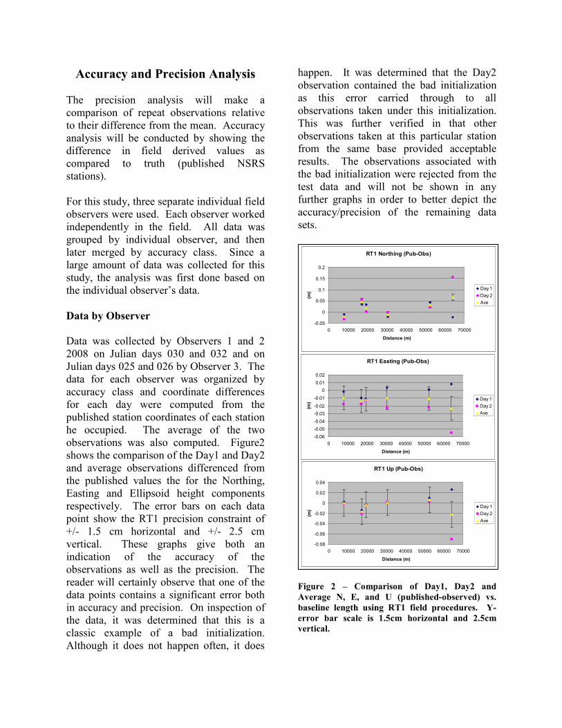
Accuracy and Precision Analysis

The precision analysis will make a

comparison of repeat observations relative

to their difference from the mean. Accuracy

analysis will be conducted by showing the

difference in field derived values as

compared to truth (published NSRS

stations).

For this study, three separate individual field

observers were used. Each observer worked

independently in the field. All data was

grouped by individual observer, and then

later merged by accuracy class. Since a

large amount of data was collected for this

study, the analysis was first done based on

the individual observer’s data.

Data by Observer

Data was collected by Observers 1 and 2

2008 on Julian days 030 and 032 and on

Julian days 025 and 026 by Observer 3. The

data for each observer was organized by

accuracy class and coordinate differences

for each day were computed from the

published station coordinates of each station

he occupied. The average of the two

observations was also computed. Figure2

shows the comparison of the Day1 and Day2

and average observations differenced from

the published values the for the Northing,

Easting and Ellipsoid height components

respectively. The error bars on each data

point show the RT1 precision constraint of

+/- 1.5 cm horizontal and +/- 2.5 cm

vertical. These graphs give both an

indication of the accuracy of the

observations as well as the precision. The

reader will certainly observe that one of the

data points contains a significant error both

in accuracy and precision. On inspection of

the data, it was determined that this is a

classic example of a bad initialization.

Although it does not happen often, it does

happen. It was determined that the Day2

observation contained the bad initialization

as this error carried through to all

observations taken under this initialization.

This was further verified in that other

observations taken at this particular station

from the same base provided acceptable

results. The observations associated with

the bad initialization were rejected from the

test data and will not be shown in any

further graphs in order to better depict the

accuracy/precision of the remaining data

sets.

Figure 2 – Comparison of Day1, Day2 and

Average N, E, and U (published-observed) vs.

baseline length using RT1 field procedures. Y-

error bar scale is 1.5cm horizontal and 2.5cm

vertical.

RT1 Northing (Pub-Obs)

-0.05

0

0.05

0.1

0.15

0.2

0 10000 20000 30000 40000 50000 60000 70000

Distance (m)

(m)

Day 1

Day 2

Ave

RT1 Easting (Pub-Obs)

-0.06

-0.05

-0.04

-0.03

-0.02

-0.01

0

0.01

0.02

0 10000 20000 30000 40000 50000 60000 70000

Distance (m)

(m)

Day 1

Day 2

Ave

RT1 Up (Pub-Obs)

-0.08

-0.06

-0.04

-0.02

0

0.02

0.04

0 10000 20000 30000 40000 50000 60000 70000

Distance (m)

(m)

Day 1

Day 2

Ave

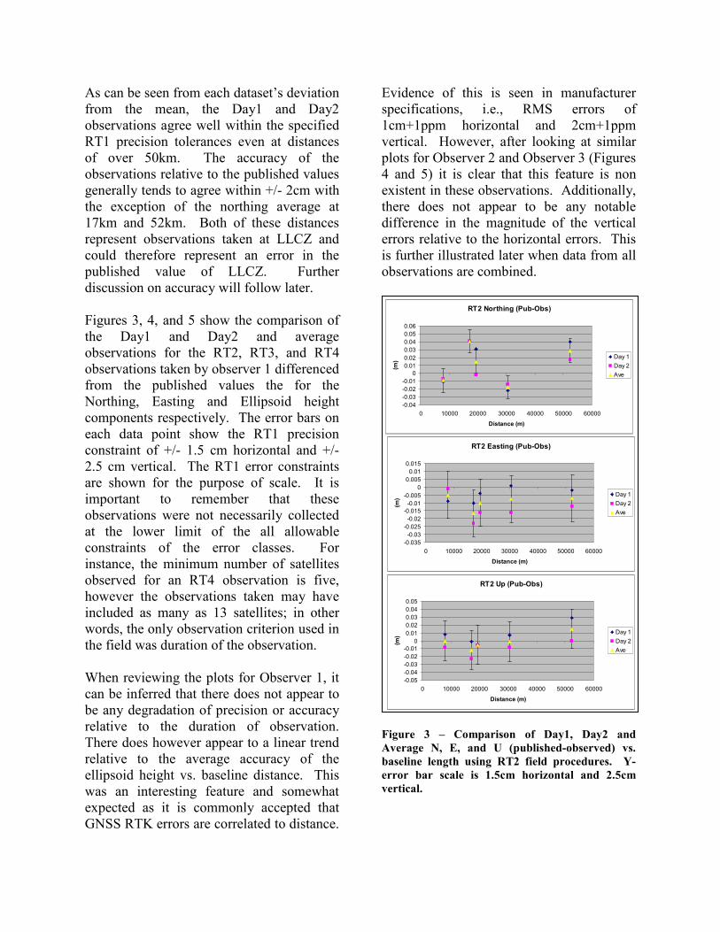
As can be seen from each dataset’s deviation

from the mean, the Day1 and Day2

observations agree well within the specified

RT1 precision tolerances even at distances

of over 50km. The accuracy of the

observations relative to the published values

generally tends to agree within +/- 2cm with

the exception of the northing average at

17km and 52km. Both of these distances

represent observations taken at LLCZ and

could therefore represent an error in the

published value of LLCZ. Further

discussion on accuracy will follow later.

Figures 3, 4, and 5 show the comparison of

the Day1 and Day2 and average

observations for the RT2, RT3, and RT4

observations taken by observer 1 differenced

from the published values the for the

Northing, Easting and Ellipsoid height

components respectively. The error bars on

each data point show the RT1 precision

constraint of +/- 1.5 cm horizontal and +/-

2.5 cm vertical. The RT1 error constraints

are shown for the purpose of scale. It is

important to remember that these

observations were not necessarily collected

at the lower limit of the all allowable

constraints of the error classes. For

instance, the minimum number of satellites

observed for an RT4 observation is five,

however the observations taken may have

included as many as 13 satellites; in other

words, the only observation criterion used in

the field was duration of the observation.

When reviewing the plots for Observer 1, it

can be inferred that there does not appear to

be any degradation of precision or accuracy

relative to the duration of observation.

There does however appear to a linear trend

relative to the average accuracy of the

ellipsoid height vs. baseline distance. This

was an interesting feature and somewhat

expected as it is commonly accepted that

GNSS RTK errors are correlated to distance.

Evidence of this is seen in manufacturer

specifications, i.e., RMS errors of

1cm+1ppm horizontal and 2cm+1ppm

vertical. However, after looking at similar

plots for Observer 2 and Observer 3 (Figures

4 and 5) it is clear that this feature is non

existent in these observations. Additionally,

there does not appear to be any notable

difference in the magnitude of the vertical

errors relative to the horizontal errors. This

is further illustrated later when data from all

observations are combined.

Figure 3 – Comparison of Day1, Day2 and

Average N, E, and U (published-observed) vs.

baseline length using RT2 field procedures. Y-

error bar scale is 1.5cm horizontal and 2.5cm

vertical.

RT2 Northing (Pub-Obs)

-0.04

-0.03

-0.02

-0.01

0

0.01

0.02

0.03

0.04

0.05

0.06

0 10000 20000 30000 40000 50000 60000

Distance (m)

(m)

Day 1

Day 2

Ave

RT2 Easting (Pub-Obs)

-0.035

-0.03

-0.025

-0.02

-0.015

-0.01

-0.005

0

0.005

0.01

0.015

0 10000 20000 30000 40000 50000 60000

Distance (m)

(m)

Day 1

Day 2

Ave

RT2 Up (Pub-Obs)

-0.05

-0.04

-0.03

-0.02

-0.01

0

0.01

0.02

0.03

0.04

0.05

0 10000 20000 30000 40000 50000 60000

Distance (m)

(m)

Day 1

Day 2

Ave

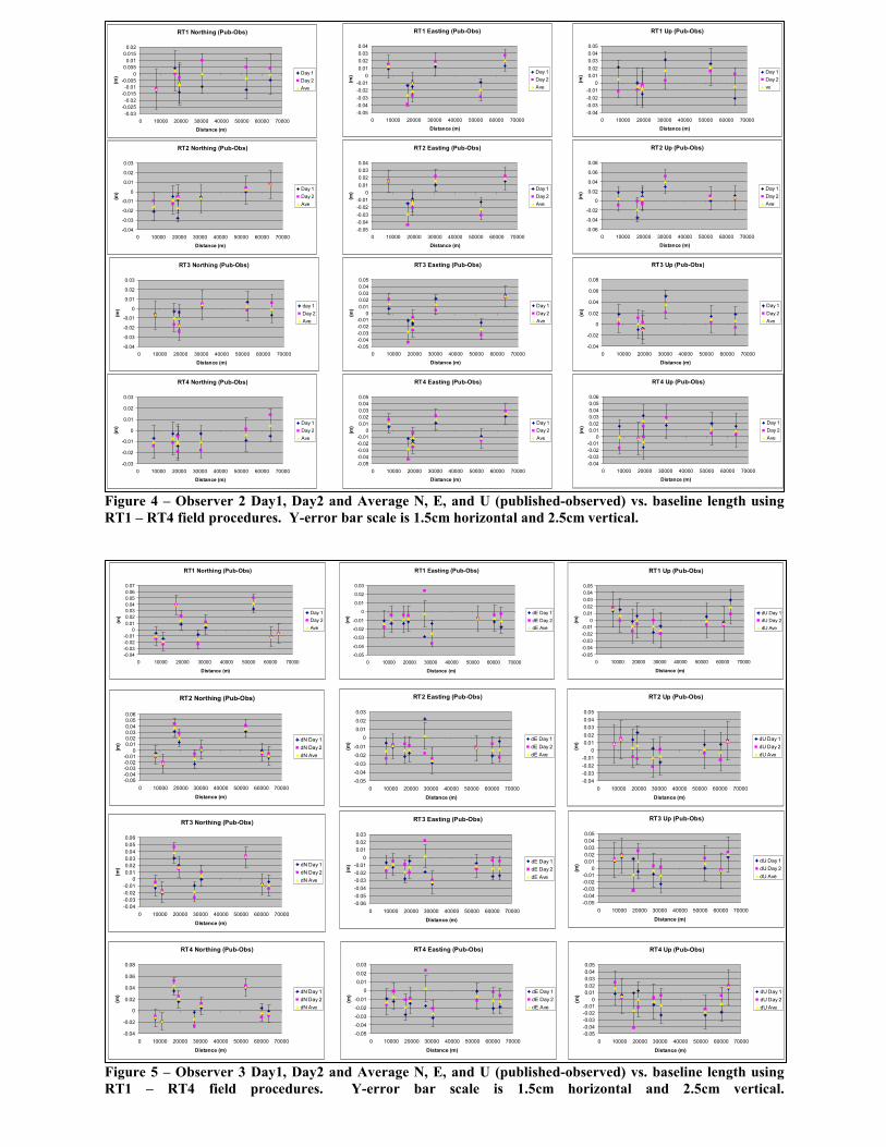
RT1 Northing (Pub-Obs)

-0.03

-0.025

-0.02

-0.015

-0.01

-0.005

0

0.005

0.01

0.015

0.02

0 10000 20000 30000 40000 50000 60000 70000

Distance (m)

(m)

Day 1

Day 2

Ave

RT1 Easting (Pub-Obs)

-0.05

-0.04

-0.03

-0.02

-0.01

0

0.01

0.02

0.03

0.04

0 10000 20000 30000 40000 50000 60000 70000

Distance (m)

(m)

Day 1

Day 2

Ave

RT1 Up (Pub-Obs)

-0.04

-0.03

-0.02

-0.01

0

0.01

0.02

0.03

0.04

0.05

0 10000 20000 30000 40000 50000 60000 70000

Distance (m)

(m)

Day 1

Day 2

ve

RT2 Northing (Pub-Obs)

-0.04

-0.03

-0.02

-0.01

0

0.01

0.02

0.03

0 10000 20000 30000 40000 50000 60000 70000

Distance (m)

(m)

Day 1

Day 2

Ave

RT2 Easting (Pub-Obs)

-0.05

-0.04

-0.03

-0.02

-0.01

0

0.01

0.02

0.03

0.04

0 10000 20000 30000 40000 50000 60000 70000

Distance (m)

(m)

Day 1

Day 2

Ave

RT2 Up (Pub-Obs)

-0.06

-0.04

-0.02

0

0.02

0.04

0.06

0.08

0 10000 20000 30000 40000 50000 60000 70000

Distance (m)

(m)

Day 1

Day 2

Ave

RT3 Northing (Pub-Obs)

-0.04

-0.03

-0.02

-0.01

0

0.01

0.02

0.03

0 10000 20000 30000 40000 50000 60000 70000

Distance (m)

(m)

day 1

Day 2

Ave

RT3 Easting (Pub-Obs)

-0.05

-0.04

-0.03

-0.02

-0.01

0

0.01

0.02

0.03

0.04

0.05

0 10000 20000 30000 40000 50000 60000 70000

Distance (m)

(m)

Day 1

Day 2

Ave

RT3 Up (Pub-Obs)

-0.04

-0.02

0

0.02

0.04

0.06

0.08

0 10000 20000 30000 40000 50000 60000 70000

Distance (m)

(m)

Day 1

Day 2

Ave

RT4 Northing (Pub-Obs)

-0.03

-0.02

-0.01

0

0.01

0.02

0.03

0 10000 20000 30000 40000 50000 60000 70000

Distance (m)

(m)

Day 1

Day 2

Ave

RT4 Easting (Pub-Obs)

-0.05

-0.04

-0.03

-0.02

-0.01

0

0.01

0.02

0.03

0.04

0.05

0 10000 20000 30000 40000 50000 60000 70000

Distance (m)

(m)

Day 1

Day 2

Ave

RT4 Up (Pub-Obs)

-0.04

-0.03

-0.02

-0.01

0

0.01

0.02

0.03

0.04

0.05

0.06

0 10000 20000 30000 40000 50000 60000 70000

Distance (m)

(m)

Day 1

Day 2

Ave

Figure 4 – Observer 2 Day1, Day2 and Average N, E, and U (published-observed) vs. baseline length using

RT1 – RT4 field procedures. Y-error bar scale is 1.5cm horizontal and 2.5cm vertical.

Figure 5 – Observer 3 Day1, Day2 and Average N, E, and U (published-observed) vs. baseline length using

RT1 – RT4 field procedures. Y-error bar scale is 1.5cm horizontal and 2.5cm vertical.

RT1 Easting (Pub-Obs)

-0.05

-0.04

-0.03

-0.02

-0.01

0

0.01

0.02

0.03

0 10000 20000 30000 40000 50000 60000 70000

Distance (m)

(m)

dE Day 1

dE Day 2

dE Ave

RT1 Northing (Pub-Obs)

-0.04

-0.03

-0.02

-0.01

0

0.01

0.02

0.03

0.04

0.05

0.06

0.07

0 10000 20000 30000 40000 50000 60000 70000

Distance (m)

(m)

Day 1

Day 2

Ave

RT2 Northing (Pub-Obs)

-0.05-0.04-0.03-0.02-0.01

0

0.010.020.030.04

0.050.06

0 10000 20000 30000 40000 50000 60000 70000

Distance (m)

(m)

dN Day 1

dN Day 2

dN Ave

RT1 Up (Pub-Obs)

-0.05

-0.04

-0.03

-0.02

-0.01

0

0.01

0.02

0.03

0.04

0.05

0 10000 20000 30000 40000 50000 60000 70000

Distance (m)

(m)

dU Day 1

dU Day 2

dU Ave

RT2 Easting (Pub-Obs)

-0.05

-0.04

-0.03

-0.02

-0.01

0

0.01

0.02

0.03

0 10000 20000 30000 40000 50000 60000 70000

Distance (m)

(m)

dE Day 1

dE Day 2

dE Ave

RT2 Up (Pub-Obs)

-0.04

-0.03

-0.02

-0.01

0

0.01

0.02

0.03

0.04

0.05

0 10000 20000 30000 40000 50000 60000 70000

Distance (m)

(m)

dU Day 1

dU Day 2

dU Ave

RT3 Northing (Pub-Obs)

-0.04

-0.03

-0.02

-0.01

0

0.01

0.02

0.03

0.04

0.05

0.06

0 10000 20000 30000 40000 50000 60000 70000

Distance (m)

(m)

dN Day 1

dN Day 2

dN Ave

RT3 Easting (Pub-Obs)

-0.06

-0.05

-0.04

-0.03

-0.02

-0.01

0

0.01

0.02

0.03

0 10000 20000 30000 40000 50000 60000 70000

Distance (m)

(m)

dE Day 1

dE Day 2

dE Ave

RT3 Up (Pub-Obs)

-0.05

-0.04

-0.03

-0.02

-0.01

0

0.01

0.02

0.03

0.04

0.05

0 10000 20000 30000 40000 50000 60000 70000

Distance (m)

(m)

dU Day 1

dU Day 2

dU Ave

RT4 Northing (Pub-Obs)

-0.04

-0.02

0

0.02

0.04

0.06

0.08

0 10000 20000 30000 40000 50000 60000 70000

Distance (m)

(m)

dN Day 1

dN Day 2

dN Ave

RT4 Easting (Pub-Obs)

-0.05

-0.04

-0.03

-0.02

-0.01

0

0.01

0.02

0.03

0 10000 20000 30000 40000 50000 60000 70000

Distance (m)

(m)

dE Day 1

dE Day 2

dE Ave

RT4 Up (Pub-Obs)

-0.05

-0.04

-0.03

-0.02

-0.01

0

0.01

0.02

0.03

0.04

0.05

0 10000 20000 30000 40000 50000 60000 70000

Distance (m)

(m)

dU Day 1

dU Day 2

dU Ave

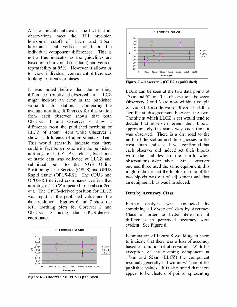
Also of notable interest is the fact that all

observations meet the RT1 precision

horizontal cutoff of 1.5cm and 2.5cm

horizontal and vertical based on the

individual component differences. This is

not a true indicator as the guidelines are

based on a horizontal (resultant) and vertical

repeatability at 95%. However it allows us

to view individual component differences

looking for trends or biases.

It was noted before that the northing

difference (published-observed) at LLCZ

might indicate an error in the published

value for this station. Comparing the

average northing differences for this station

from each observer shows that both

Observer 1 and Observer 3 show a

difference from the published northing of

LLCZ of about +4cm while Observer 2

shows a difference of approximately -1cm.

This would generally indicate that there

could in fact be an issue with the published

northing for LLCZ. As a check, two hours

of static data was collected at LLCZ and

submitted both to the NGS Online

Positioning User Service (OPUS) and OPUS

Rapid Static (OPUS-RS). The OPUS and

OPUS-RS derived coordinates verified that

northing of LLCZ appeared to be about 2cm

out. The OPUS-derived position for LLCZ

was input as the published value and the

data replotted. Figures 6 and 7 show the

RT1 northing plots for Observer 2 and

Observer 3 using the OPUS-derived

coordinate.

RT1 Northing (Pub-Obs)

-0.045

-0.04

-0.035

-0.03

-0.025

-0.02

-0.015

-0.01

-0.005

0

0.005

0 10000 20000 30000 40000 50000 60000 70000

Distance (m)

(m)

Day 1

Day 2

Ave

Figure 6 – Observer 2 (OPUS as published)

RT1 Northing (Pub-Obs)

-0.05

-0.04

-0.03

-0.02

-0.01

0

0.01

0.02

0.03

0.04

0.05

0 10000 20000 30000 40000 50000 60000 70000

Distance (m)

(m)

Day 1

Day 2

Ave

Figure 7 – Observer 3 (OPUS as published)

LLCZ can be seen at the two data points at

17km and 52km. The observations between

Observers 2 and 3 are now within a couple

of cm of truth however there is still a

significant disagreement between the two.

The site at which LLCZ is set would tend to

dictate that observers orient their bipods

approximately the same way each time it

was observed. There is a dirt road to the

north of the station and thick grasses to the

west, south, and east. It was confirmed that

each observer did indeed set their bipods

with the bubbles to the north when

observations were taken. Since observer

one and three used the same equipment, this

might indicate that the bubble on one of the

two bipods was out of adjustment and that

an equipment bias was introduced.

Data by Accuracy Class

Further analysis was conducted by

combining all observers’ data by Accuracy

Class in order to better determine if

differences in perceived accuracy were

evident. See Figure 8.

Examination of Figure 8 would again seem

to indicate that there was a loss of accuracy

based on duration of observation. With the

exception of the northing component at

17km and 52km (LLCZ) the component

residuals generally fall within +/- 2cm of the

published values. It is also noted that there

appear to be clusters of points representing

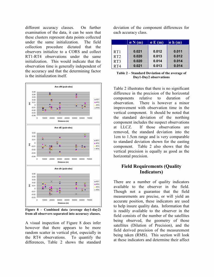
different accuracy classes. On further

examination of the data, it can be seen that

these clusters represent data points collected

under the same initialization. The field

collection procedure dictated that the

observers initialize to a CORS and collect

RT1-RT4 observations under the same

initialization. This would indicate that the

observation time is generally independent of

the accuracy and that the determining factor

is the initialization itself.

Figure 8 – Combined data (average day1-day2)

from all observers separated into accuracy classes.

A visual inspection of Figure 8 does infer

however that there appears to be more

random scatter in vertical plot, especially in

the RT4 observations. To quantify the

differences, Table 2 shows the standard

deviation of the component differences for

each accuracy class.

σ N (m) σ E (m) σ h (m)

RT1 0.021 0.012 0.011

RT2 0.020 0.013 0.012

RT3 0.020 0.014 0.014

RT4 0.021 0.013 0.014

Table 2 – Standard Deviation of the average of

Day1-Day2 observations

Table 2 illustrates that there is no significant

difference in the precision of the horizontal

components relative to duration of

observation. There is however a minor

improvement with observation time in the

vertical component. It should be noted that

the standard deviation of the northing

component includes the suspect observations

at LLCZ. If those observations are

removed, the standard deviation into the

1cm to 1.5cm range and is very comparable

to standard deviation shown for the easting

component. Table 2 also shows that the

vertical precision is equally as good as the

horizontal precision.

Field Requirements (Quality

Indicators)

There are a number of quality indicators

available to the observer in the field.

Though not a guarantee that the field

measurements are precise, or will yield an

accurate position, these indicators are used

to help insure quality data. Information that

is readily available to the observer in the

field consists of the number of the satellites

being observed, the geometry of those

satellites (Dilution of Precision), and the

field derived precision of the measurement

being taken (RMS). This section will look

at these indicators and determine their affect

Ave dN (pub-obs)

-0.04

-0.03

-0.02

-0.01

0

0.01

0.02

0.03

0.04

0.05

0 10000 20000 30000 40000 50000 60000 70000

Distance (m)

(m)

RT1

RT2

RT3

RT4

Ave dE (pub-obs)

-0.04

-0.03

-0.02

-0.01

0

0.01

0.02

0.03

0 10000 20000 30000 40000 50000 60000 70000

Distance (m)

(m)

RT1

RT2

RT3

RT4

Ave dh (pub-obs)

-0.03

-0.02

-0.01

0

0.01

0.02

0.03

0.04

0.05

0 10000 20000 30000 40000 50000 60000 70000

Distance (m)

(m)

RT1

RT2

RT3

RT4

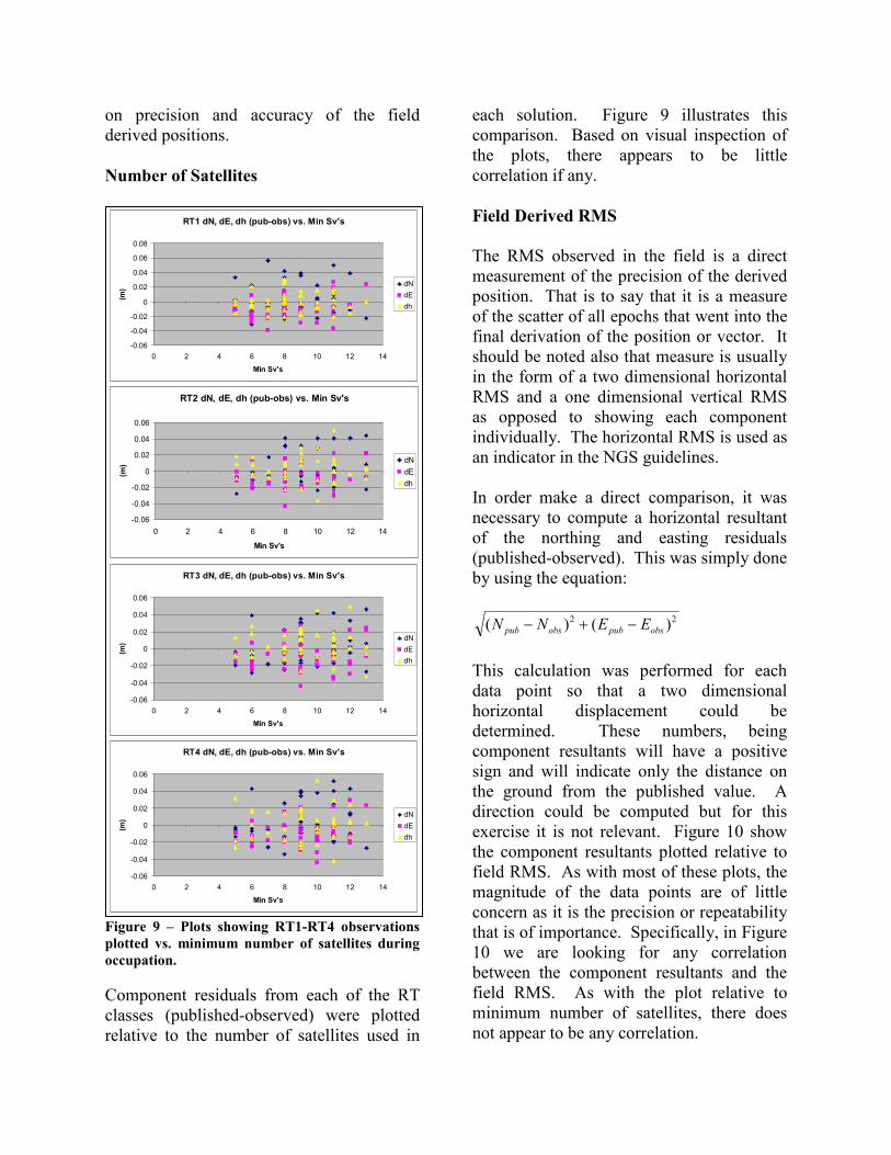
on precision and accuracy of the field

derived positions.

Number of Satellites

Figure 9 – Plots showing RT1-RT4 observations

plotted vs. minimum number of satellites during

occupation.

Component residuals from each of the RT

classes (published-observed) were plotted

relative to the number of satellites used in

each solution. Figure 9 illustrates this

comparison. Based on visual inspection of

the plots, there appears to be little

correlation if any.

Field Derived RMS

The RMS observed in the field is a direct

measurement of the precision of the derived

position. That is to say that it is a measure

of the scatter of all epochs that went into the

final derivation of the position or vector. It

should be noted also that measure is usually

in the form of a two dimensional horizontal

RMS and a one dimensional vertical RMS

as opposed to showing each component

individually. The horizontal RMS is used as

an indicator in the NGS guidelines.

In order make a direct comparison, it was

necessary to compute a horizontal resultant

of the northing and easting residuals

(published-observed). This was simply done

by using the equation:

22 )()( obspubobspub EENN −+−

This calculation was performed for each

data point so that a two dimensional

horizontal displacement could be

determined. These numbers, being

component resultants will have a positive

sign and will indicate only the distance on

the ground from the published value. A

direction could be computed but for this

exercise it is not relevant. Figure 10 show

the component resultants plotted relative to

field RMS. As with most of these plots, the

magnitude of the data points are of little

concern as it is the precision or repeatability

that is of importance. Specifically, in Figure

10 we are looking for any correlation

between the component resultants and the

field RMS. As with the plot relative to

minimum number of satellites, there does

not appear to be any correlation.

RT1 dN, dE, dh (pub-obs) vs. Min Sv's

-0.06

-0.04

-0.02

0

0.02

0.04

0.06

0.08

0 2 4 6 8 10 12 14

Min Sv's

(m)

dN

dE

dh

RT2 dN, dE, dh (pub-obs) vs. Min Sv's

-0.06

-0.04

-0.02

0

0.02

0.04

0.06

0 2 4 6 8 10 12 14

Min Sv's

(m)

dN

dE

dh

RT3 dN, dE, dh (pub-obs) vs. Min Sv's

-0.06

-0.04

-0.02

0

0.02

0.04

0.06

0 2 4 6 8 10 12 14

Min Sv's

(m)

dN

dE

dh

RT4 dN, dE, dh (pub-obs) vs. Min Sv's

-0.06

-0.04

-0.02

0

0.02

0.04

0.06

0 2 4 6 8 10 12 14

Min Sv's

(m)

dN

dE

dh

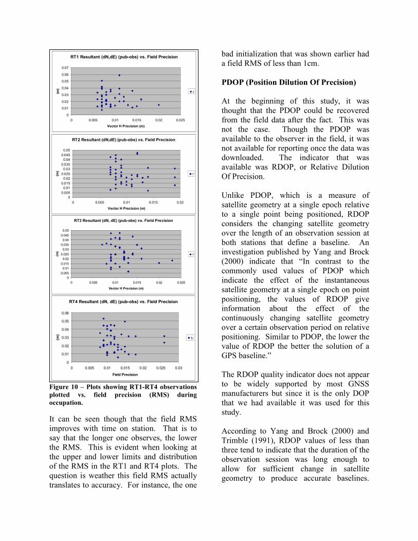
Figure 10 – Plots showing RT1-RT4 observations

plotted vs. field precision (RMS) during

occupation.

It can be seen though that the field RMS

improves with time on station. That is to

say that the longer one observes, the lower

the RMS. This is evident when looking at

the upper and lower limits and distribution

of the RMS in the RT1 and RT4 plots. The

question is weather this field RMS actually

translates to accuracy. For instance, the one

bad initialization that was shown earlier had

a field RMS of less than 1cm.

PDOP (Position Dilution Of Precision)

At the beginning of this study, it was

thought that the PDOP could be recovered

from the field data after the fact. This was

not the case. Though the PDOP was

available to the observer in the field, it was

not available for reporting once the data was

downloaded. The indicator that was

available was RDOP, or Relative Dilution

Of Precision.

Unlike PDOP, which is a measure of

satellite geometry at a single epoch relative

to a single point being positioned, RDOP

considers the changing satellite geometry

over the length of an observation session at

both stations that define a baseline. An

investigation published by Yang and Brock

(2000) indicate that “In contrast to the

commonly used values of PDOP which

indicate the effect of the instantaneous

satellite geometry at a single epoch on point

positioning, the values of RDOP give

information about the effect of the

continuously changing satellite geometry

over a certain observation period on relative

positioning. Similar to PDOP, the lower the

value of RDOP the better the solution of a

GPS baseline.”

The RDOP quality indicator does not appear

to be widely supported by most GNSS

manufacturers but since it is the only DOP

that we had available it was used for this

study.

According to Yang and Brock (2000) and

Trimble (1991), RDOP values of less than

three tend to indicate that the duration of the

observation session was long enough to

allow for sufficient change in satellite

geometry to produce accurate baselines.

RT1 Resultant (dN,dE) (pub-obs) vs. Field Precision

0

0.01

0.02

0.03

0.04

0.05

0.06

0.07

0 0.005 0.01 0.015 0.02 0.025

Vector H Precision (m)

(m)

r

RT2 Resultant (dN,dE) (pub-obs) vs. Field Precision

0

0.005

0.01

0.015

0.02

0.025

0.03

0.035

0.04

0.045

0.05

0 0.005 0.01 0.015 0.02

Vector H Precision (m)

(m)

r

RT3 Resultant (dN, dE) (pub-obs) vs. Field Precision

0

0.005

0.01

0.015

0.02

0.025

0.03

0.035

0.04

0.045

0.05

0 0.005 0.01 0.015 0.02 0.025

Vector H Precision (m)

(m)

r

RT4 Resultant (dN, dE) (pub-obs) vs. Field Precision

0

0.01

0.02

0.03

0.04

0.05

0.06

0 0.005 0.01 0.015 0.02 0.025 0.03

Field Precision

(m)

h

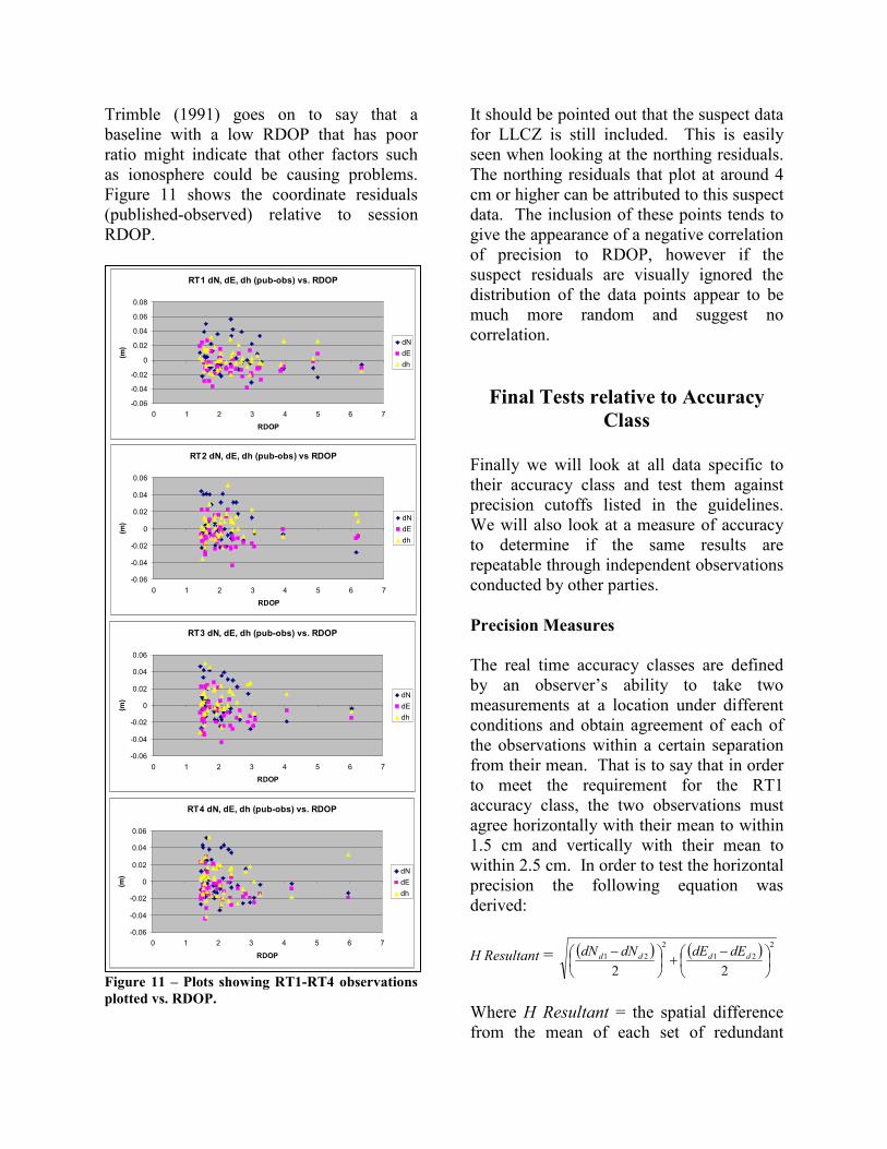
Trimble (1991) goes on to say that a

baseline with a low RDOP that has poor

ratio might indicate that other factors such

as ionosphere could be causing problems.

Figure 11 shows the coordinate residuals

(published-observed) relative to session

RDOP.

Figure 11 – Plots showing RT1-RT4 observations

plotted vs. RDOP.

It should be pointed out that the suspect data

for LLCZ is still included. This is easily

seen when looking at the northing residuals.

The northing residuals that plot at around 4

cm or higher can be attributed to this suspect

data. The inclusion of these points tends to

give the appearance of a negative correlation

of precision to RDOP, however if the

suspect residuals are visually ignored the

distribution of the data points appear to be

much more random and suggest no

correlation.

Final Tests relative to Accuracy

Class

Finally we will look at all data specific to

their accuracy class and test them against

precision cutoffs listed in the guidelines.

We will also look at a measure of accuracy

to determine if the same results are

repeatable through independent observations

conducted by other parties.

Precision Measures

The real time accuracy classes are defined

by an observer’s ability to take two

measurements at a location under different

conditions and obtain agreement of each of

the observations within a certain separation

from their mean. That is to say that in order

to meet the requirement for the RT1

accuracy class, the two observations must

agree horizontally with their mean to within

1.5 cm and vertically with their mean to

within 2.5 cm. In order to test the horizontal

precision the following equation was

derived:

H Resultant = ( ) ( ) 2

21

2

21

22

−+

− dddd dEdEdNdN

Where H Resultant = the spatial difference

from the mean of each set of redundant

RT1 dN, dE, dh (pub-obs) vs. RDOP

-0.06

-0.04

-0.02

0

0.02

0.04

0.06

0.08

0 1 2 3 4 5 6 7

RDOP

(m)

dN

dE

dh

RT2 dN, dE, dh (pub-obs) vs RDOP

-0.06

-0.04

-0.02

0

0.02

0.04

0.06

0 1 2 3 4 5 6 7

RDOP

(m)

dN

dE

dh

RT3 dN, dE, dh (pub-obs) vs. RDOP

-0.06

-0.04

-0.02

0

0.02

0.04

0.06

0 1 2 3 4 5 6 7

RDOP

(m)

dN

dE

dh

RT4 dN, dE, dh (pub-obs) vs. RDOP

-0.06

-0.04

-0.02

0

0.02

0.04

0.06

0 1 2 3 4 5 6 7

RDOP

(m)

dN

dE

dh

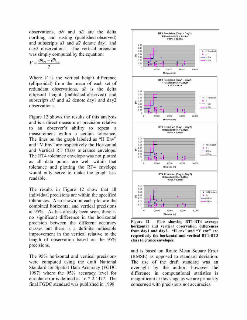
observations, dN and dE are the delta

northing and easting (published-observed)

and subscripts d1 and d2 denote day1 and

day2 observations. The vertical precision

was simply computed by the equation:

2

21 dd dhdhV

−=

Where V is the vertical height difference

(ellipsoidal) from the mean of each set of

redundant observations, dh is the delta

ellipsoid height (published-observed) and

subscripts d1 and d2 denote day1 and day2

observations.

Figure 12 shows the results of this analysis

and is a direct measure of precision relative

to an observer’s ability to repeat a

measurement within a certain tolerance.

The lines on the graph labeled as “H Env”

and “V Env” are respectively the Horizontal

and Vertical RT Class tolerance envelope.

The RT4 tolerance envelope was not plotted

as all data points are well within that

tolerance and plotting the RT4 envelope

would only serve to make the graph less

readable.

The results in Figure 12 show that all

individual precisions are within the specified

tolerances. Also shown on each plot are the

combined horizontal and vertical precisions

at 95%. As has already been seen, there is

no significant difference in the horizontal

precision between the different accuracy

classes but there is a definite noticeable

improvement in the vertical relative to the

length of observation based on the 95%

precisions.

The 95% horizontal and vertical precisions

were computed using the draft National

Standard for Spatial Data Accuracy (FGDC

1997) where the 95% accuracy level for

circular error is defined as 1σ * 2.4477. The

final FGDC standard was published in 1998

Figure 12 – Plots showing RT1-RT4 average

horizontal and vertical observation differences

from day1 and day2. “H env” and “V env” are

respectively the horizontal and vertical RT1-RT3

class tolerance envelopes.

and is based on Route Mean Square Error

(RMSE) as opposed to standard deviation.

The use of the draft standard was an

oversight by the author; however the

difference in computational statistics is

insignificant at this stage as we are primarily

concerned with precisions not accuracies.

RT1 Precision (Day1 - Day2)H Resultant 95% = 0.014m

V 95% = 0.009m

0

0.01

0.02

0.03

0.04

0.05

0.06

0.07

0 20000 40000 60000 80000

Distance (m)

(m)

H Resultant

h

H Env

V Env

RT2 Precision (Day1 - Day2)H Resultand 95% = 0.012m

V 95% = 0.010

0

0.01

0.02

0.03

0.04

0.05

0.06

0.07

0 20000 40000 60000 80000

Distance (m)

(m)

H Resultant

h

H Env

V Env

RT3 Precision (Day1 - Day2)H Resultant 95% = 0.012m

V 95% = 0.012m

0

0.01

0.02

0.03

0.04

0.05

0.06

0.07

0 20000 40000 60000 80000

Distance (m)

(m)

H Resultant

h

H Env

V Env

RT4 Precision (Day1 - Day2)H Resultant 95% = 0.013m

V 95% = 0.016m

0

0.01

0.02

0.03

0.04

0.05

0.06

0.07

0 20000 40000 60000 80000

Distance (m)

(m)

H Resultant

h

H Env

V Env

Transitioning Precision Measures to

Accuracy Measures

The accuracy of a measurement is defined

by how closely the measurement compares

to truth. In this case study, measurements

were taken at points with know coordinates

so accuracy can be tested by comparing our

measurements to these known values. More

importantly, we can measure the scatter of

the data for each accuracy class collected by

different observers. By doing this, we can

determine any observer’s ability to be within

some statistical horizontal radius and

vertical separation from each other. In lieu

of a known value, the average of all

observers’ measurements would best

represent truth. Figure 13 shows the average

radial error for each observation set (Day1,

Day2). Figure 14 shows the corresponding

average vertical error for each observation

set.

Horizontal Resultant (pub-obs) Average Day1-Day2

0

0.01

0.02

0.03

0.04

0.05

0.06

0 10000 20000 30000 40000 50000 60000 70000

Distance (m)

(m)

RT1r

RT2r

RT3r

RT4r

Figure 13 – Plot showing RT1-RT4 average radial

error (Published – Average Day1, Day2).

dh (pub-obs) Average Day1-Day2

-0.03

-0.02

-0.01

0

0.01

0.02

0.03

0.04

0.05

0 10000 20000 30000 40000 50000 60000 70000

Distance (m)

(m)

RT1h

RT2h

RT3h

RT4h

Figure 14 – Plot showing RT1-RT4 average

vertical error (published – Average Day1, Day2).

As before, the larger residuals at LLCZ have

been left in the analysis but as previously

indicated, these observations may contain an

equipment bias. Table 3 shows the

horizontal and vertical 2σ error estimates

from the data contained in figures 13 and 14.

2σ Horizontal

(m)

2σ Vertical

(m)

RT1 0.024663 0.020933

RT2 0.021754 0.023475

RT3 0.020684 0.027002

RT4 0.025223 0.027488

Table 3 – Horizontal and Vertical 2σ Error

Estimates (Average of Day1-Day2 observations)

Table 4 shows the horizontal 2σ error

estimates if the large residuals at LLCZ are

removed from the analysis.

2σ Horizontal (m)

RT1 0.010786

RT2 0.011772

RT3 0.013639

RT4 0.014448

Table 4 – Horizontal 2σ Error Estimates (Average

of Day1-Day2 observations) with Large LLCZ

Residuals Removed

Tables 3 and 4 are showing the observers’

ability to produce the same radial error. For

instance, table 4 indicates that observations

taken under RT1 criterion will produce a

radial error that is within 0.011 meters of

similar observations 95% of the time. These

numbers directly correspond to the expected

accuracy of one observer’s coordinate

determination relative to another observer’

coordinate determination.

As was seen previously, the precision of the

vertical component decreases slightly as

observations are shortened. Also, now that

the suspect data at LLCZ has been removed

(Table 4), a slight decrease in horizontal

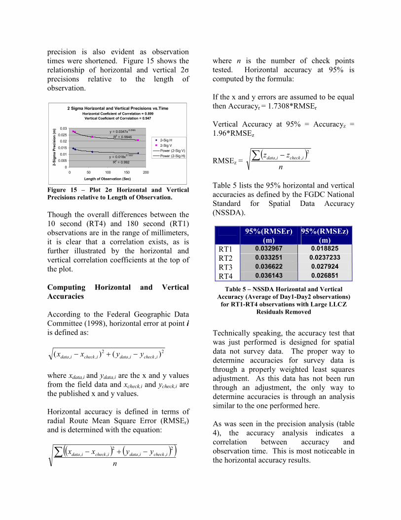
precision is also evident as observation

times were shortened. Figure 15 shows the

relationship of horizontal and vertical 2σ

precisions relative to the length of

observation.

2 Sigma Horizontal and Vertical Precisions vs.Time

Horizontal Coeficient of Correlation = 0.899

Vertical Coeficient of Correlation = 0.947

y = 0.0347x-0.0965

R2 = 0.9946

y = 0.018x-0.1007

R2 = 0.992

0

0.005

0.01

0.015

0.02

0.025

0.03

0 50 100 150 200

Length of Observation (Sec)

2-Sigma Precision (m)

2-Sig H

2-Sig V

Power (2-Sig V)

Power (2-Sig H)

Figure 15 – Plot 2σ Horizontal and Vertical

Precisions relative to Length of Observation.

Though the overall differences between the

10 second (RT4) and 180 second (RT1)

observations are in the range of millimeters,

it is clear that a correlation exists, as is

further illustrated by the horizontal and

vertical correlation coefficients at the top of

the plot.

Computing Horizontal and Vertical

Accuracies

According to the Federal Geographic Data

Committee (1998), horizontal error at point i

is defined as:

2

,,

2

,, )()( icheckidataicheckidata yyxx −+−

where xdata,i and ydata,i are the x and y values

from the field data and xcheck,i and ycheck,i are

the published x and y values.

Horizontal accuracy is defined in terms of

radial Route Mean Square Error (RMSEr)

and is determined with the equation:

( ) ( )( )n

yyxx icheckidataicheckidata∑ −+− 2

,,

2

,,

where n is the number of check points

tested. Horizontal accuracy at 95% is

computed by the formula:

If the x and y errors are assumed to be equal

then Accuracyr = 1.7308*RMSEr

Vertical Accuracy at 95% = Accuracyz =

1.96*RMSEz

RMSEz = ( )

n

zz icheckidata∑ − 2

,,

Table 5 lists the 95% horizontal and vertical

accuracies as defined by the FGDC National

Standard for Spatial Data Accuracy

(NSSDA).

95%(RMSEr)

(m)

95%(RMSEz)

(m)

RT1 0.032967 0.018825

RT2 0.033251 0.0237233

RT3 0.036622 0.027924

RT4 0.036143 0.026851

Table 5 – NSSDA Horizontal and Vertical

Accuracy (Average of Day1-Day2 observations)

for RT1-RT4 observations with Large LLCZ

Residuals Removed

Technically speaking, the accuracy test that

was just performed is designed for spatial

data not survey data. The proper way to

determine accuracies for survey data is

through a properly weighted least squares

adjustment. As this data has not been run

through an adjustment, the only way to

determine accuracies is through an analysis

similar to the one performed here.

As was seen in the precision analysis (table

4), the accuracy analysis indicates a

correlation between accuracy and

observation time. This is most noticeable in

the horizontal accuracy results.

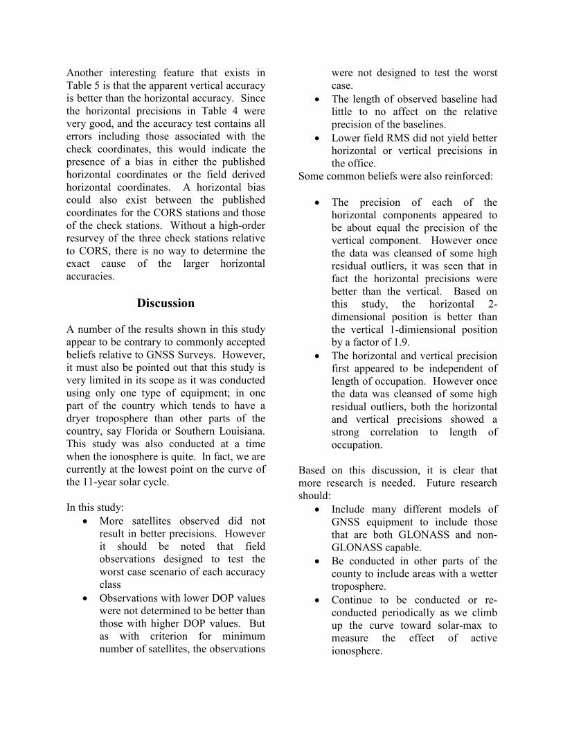
Another interesting feature that exists in

Table 5 is that the apparent vertical accuracy

is better than the horizontal accuracy. Since

the horizontal precisions in Table 4 were

very good, and the accuracy test contains all

errors including those associated with the

check coordinates, this would indicate the

presence of a bias in either the published

horizontal coordinates or the field derived

horizontal coordinates. A horizontal bias

could also exist between the published

coordinates for the CORS stations and those

of the check stations. Without a high-order

resurvey of the three check stations relative

to CORS, there is no way to determine the

exact cause of the larger horizontal

accuracies.

Discussion

A number of the results shown in this study

appear to be contrary to commonly accepted

beliefs relative to GNSS Surveys. However,

it must also be pointed out that this study is

very limited in its scope as it was conducted

using only one type of equipment; in one

part of the country which tends to have a

dryer troposphere than other parts of the

country, say Florida or Southern Louisiana.

This study was also conducted at a time

when the ionosphere is quite. In fact, we are

currently at the lowest point on the curve of

the 11-year solar cycle.

In this study:

• More satellites observed did not

result in better precisions. However

it should be noted that field

observations designed to test the

worst case scenario of each accuracy

class

• Observations with lower DOP values

were not determined to be better than

those with higher DOP values. But

as with criterion for minimum

number of satellites, the observations

were not designed to test the worst

case.

• The length of observed baseline had

little to no affect on the relative

precision of the baselines.

• Lower field RMS did not yield better

horizontal or vertical precisions in

the office.

Some common beliefs were also reinforced:

• The precision of each of the

horizontal components appeared to

be about equal the precision of the

vertical component. However once

the data was cleansed of some high

residual outliers, it was seen that in

fact the horizontal precisions were

better than the vertical. Based on

this study, the horizontal 2-

dimensional position is better than

the vertical 1-dimiensional position

by a factor of 1.9.

• The horizontal and vertical precision

first appeared to be independent of

length of occupation. However once

the data was cleansed of some high

residual outliers, both the horizontal

and vertical precisions showed a

strong correlation to length of

occupation.

Based on this discussion, it is clear that

more research is needed. Future research

should:

• Include many different models of

GNSS equipment to include those

that are both GLONASS and non-

GLONASS capable.

• Be conducted in other parts of the

county to include areas with a wetter

troposphere.

• Continue to be conducted or re-

conducted periodically as we climb

up the curve toward solar-max to

measure the effect of active

ionosphere.

Conclusions

As the use of RTK positioning continues to

increase, so does the need for development

of standards, specifications, and guidelines

designed to meet specific levels of precision

and accuracy. The results shown in this case

study are very encouraging relative to the

ability to produce observations of high

precision with “Single Base RTK”. In fact

the results far exceeded the author’s

expectations relative to the NGS Accuracy

Classes. Further research may show that

some of the observation criterion listed such

as minimum number of satellites, PDOP,

and RMS may be relaxed or may be shown

to have little to no effect on one’s ability to

produce precise RTK measurements.

The case study reported here shows that

Single Base RTK observations can be taken

over significantly long distances up to (60

km) and still produce results that meet or

approach the precision levels of much

shorter observations. It is also shown that

the duration or length of observation is a

definite factor in the precision of RTK

measurements. Finally, it can be concluded

that if:

• Observations are designed with

proper redundancy to remove

systematic errors (tropo, iono) and

detect bad initializations;

• The data is analyzed to detect and

remove statistical outliers;

Single Base RTK observations that meet or

exceed the precision criterion of the NGS

Single Base Guidelines for RT1, RT2, RT3,

and RT4 accuracy classes is achievable

carried out under normal field conditions

similar to those experienced during this case

study.

References

FGCD. 1997. Draft Geospatial Positioning

Accuracy Standards Part 3: National

Standard for Spatial Data Accuracy. May

1997. Federal Geographic Data Committee,

590 National Center, Reston, VA, 20192

Federal Geographic Data Committee. 1998.

Geospatial Positioning Accuracy Standards

Part 3: National Standard for Spatial Data

Accuracy. 1998. Federal Geographic Data

Committee, 590 National Center, Reston,

VA, 20192

Trimble 1991. Trimvec-Plus GPS Survey

Software, User’s Manual and Technical

Reference Guide. September, 1991, P 3-12.

Yang, X., and R. Brock. 2000. RDOP

Surface for GPS Relative Positioning.

United States Patent Claim 6057800,

[http://www.patentstory.us/patents/6057800

-fulltext.html]

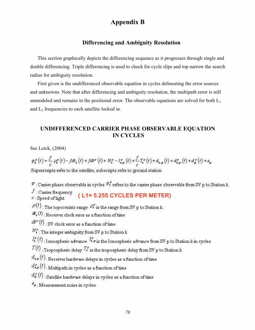
78

Appendix B

Differencing and Ambiguity Resolution This section graphically depicts the differencing sequence as it progresses through single and

double differencing. Triple differencing is used to check for cycle slips and top narrow the search

radius for ambiguity resolution.

First given is the undifferenced observable equation in cycles delineating the error sources

and unknowns. Note that after differencing and ambiguity resolution, the multipath error is still

unmodeled and remains in the positional error. The observable equations are solved for both L1

and L2 frequencies to each satellite locked in. UNDIFFERENCED CARRIER PHASE OBSERVABLE EQUATION

IN CYCLES

See Leick, (2004)

( L1= 5.255 CYCLES PER METER)

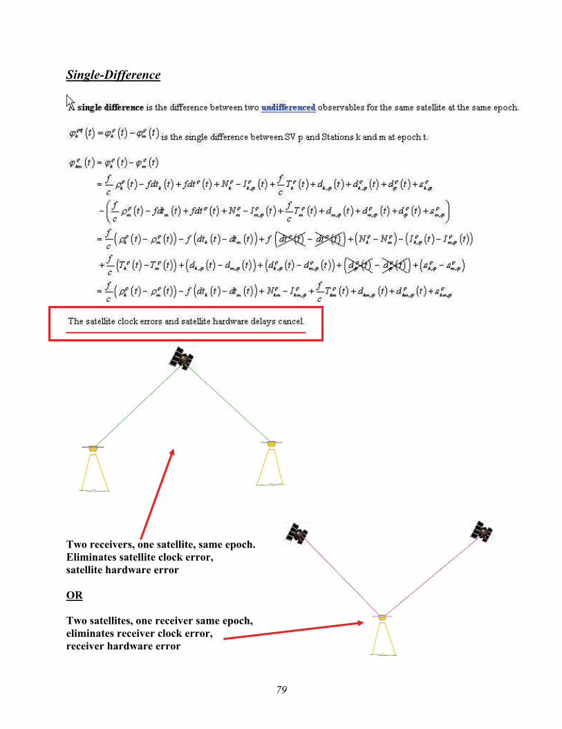
79

Single-Difference

Two receivers, one satellite, same epoch. Eliminates satellite clock error, satellite hardware error OR Two satellites, one receiver same epoch, eliminates receiver clock error, receiver hardware error

80

Double-Differenced Phase Solution

Double differencing: two receivers, two satellites, same epoch (two Single Differences). Eliminates receiver clock error, receiver hardware error, reduces other errors

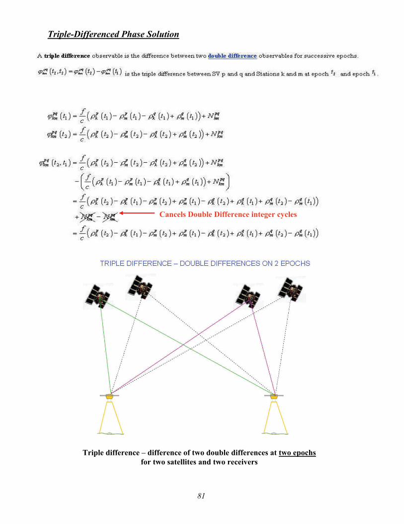
81

Triple-Differenced Phase Solution

Triple difference – difference of two double differences at two epochs for two satellites and two receivers

Cancels Double Difference integer cycles

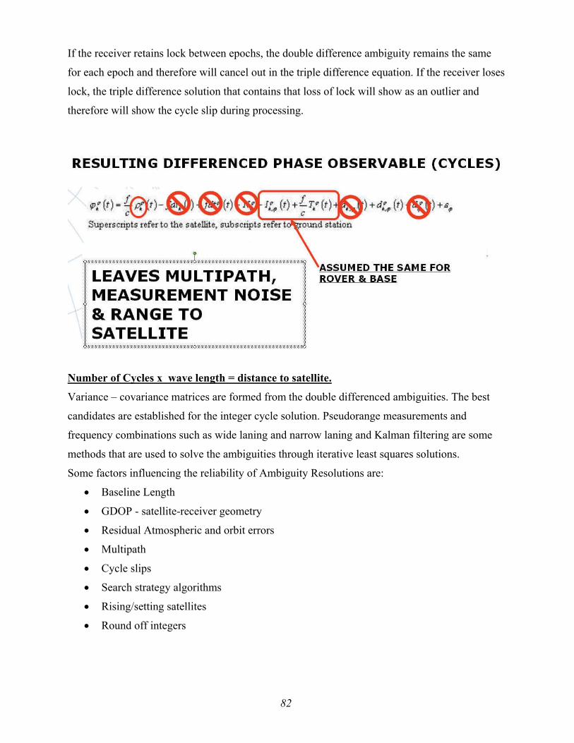
82

If the receiver retains lock between epochs, the double difference ambiguity remains the same

for each epoch and therefore will cancel out in the triple difference equation. If the receiver loses

lock, the triple difference solution that contains that loss of lock will show as an outlier and

therefore will show the cycle slip during processing.

Number of Cycles x wave length = distance to satellite.

Variance – covariance matrices are formed from the double differenced ambiguities. The best

candidates are established for the integer cycle solution. Pseudorange measurements and

frequency combinations such as wide laning and narrow laning and Kalman filtering are some

methods that are used to solve the ambiguities through iterative least squares solutions.

Some factors influencing the reliability of Ambiguity Resolutions are:

• Baseline Length

• GDOP - satellite-receiver geometry

• Residual Atmospheric and orbit errors

• Multipath

• Cycle slips

• Search strategy algorithms

• Rising/setting satellites

• Round off integers

83

Statistically, the ratio of the best to next best solution is constantly monitored in conjunction

with change or increase in the RMS. This then gives assurance of the correct ambiguity

resolution as the session proceeds after initialization to a fixed solution. Most major GNSS

hardware/software manufacturers give their ambiguity resolution confidence at 99.9 percent.