Using Low-energy 8Li Beta-detected NMR to Probe the ...
190
Using Low-energy 8 Li Beta-detected NMR to Probe the Magnetism of Transition Metals by Terry J. Parolin B.Sc., McGill University, 2000 M.S., CarnegieMellon University, 2002 A THESIS SUBMITTED IN PARTIAL FULFILLMENT OF THE REQUIREMENTS FOR THE DEGREE OF DOCTOR OF PHILOSOPHY in The Faculty of Graduate Studies (Chemistry) THE UNIVERSITY OF BRITISH COLUMBIA (Vancouver) December, 2011 c Terry J. Parolin 2011
Transcript of Using Low-energy 8Li Beta-detected NMR to Probe the ...
Using Low-energy 8Li Beta-detectedNMR to Probe the Magnetism of
Transition Metalsby
Terry J. Parolin
B.Sc., McGill University, 2000M.S., CarnegieMellon University, 2002
A THESIS SUBMITTED IN PARTIAL FULFILLMENT OFTHE REQUIREMENTS FOR THE DEGREE OF
DOCTOR OF PHILOSOPHY
in
The Faculty of Graduate Studies
(Chemistry)
THE UNIVERSITY OF BRITISH COLUMBIA
(Vancouver)
December, 2011
c© Terry J. Parolin 2011
Abstract
Low-energy, beta-radiation-detected nuclear magnetic resonance (β-NMR)
is applied to probe the magnetism of Au and Pd. The measurements were
carried out at the TRIUMF β-NMR facility using optically spin-polarized8Li+ as the probe.
The behaviour of 8Li+ in Au was investigated using samples in the form
of a foil and a 100 nm film evaporated onto a MgO (100) substrate. The re-
sults are in overall agreement with those obtained previously in Ag, Cu, and
Al. Narrow, temperature-independent resonances are observed and assigned
to ions stopping in the octahedral interstitial and substitutional lattice sites;
the latter appearing only for temperatures above 150 K which is attributed
to a thermally-activated site change. The spin-lattice relaxation rate of sub-
stitutional site ions is less than half as fast at ambient temperature as that
in the other simple metals. The rate is independent of external field for
fields greater than 15 mT. A Korringa analysis for the substitutional ions
indicates no significant electron enhancement over that of a free electron
gas. For all four metals, the enhancements obtained are smaller than those
for the host nuclei. No depth dependence was found for the resonances in
Au.
The highly exchange-enhanced metal Pd was studied using samples in
the form of a foil and a 100 nm film evaporated onto a SrTiO3 (100) sub-
strate. Strongly temperature-dependent, negative shifts are observed that
scale with the temperature dependence of the host susceptibility between
room temperature and 110 K. The resonances appear as two partially re-
solved lines that exhibit similar behaviour with temperature. The linewidths
are broad and double upon cooling. The data are indicative of ions stop-
ping in a site of cubic symmetry. The spin-lattice relaxation rate increases
ii
Abstract
linearly with increasing temperature and eventually saturates at higher tem-
peratures, consistent with the prediction from spin fluctuation theory. In
contrast to the simple metals, large Korringa enhancements are obtained in
this host. Ferromagnetic dynamical scaling is observed to hold above 110
K. Features below this temperature indicate that the Li ions locally induce
a further enhancement of the static susceptibility. The temperature depen-
dence of the modified susceptibility is in keeping with the prediction for
a weak itinerant ferromagnet just above the Curie temperature; however,
there is no evidence of static order.
iii
Preface
A figure in Chapter 2 contains data that has been published: T.J. Parolin,
J. Shi, Z. Salman, K.H. Chow, P. Dosanjh, H. Saadaoui, Q. Song, M.D.
Hossain, R.F. Kiefl, C.D.P. Levy, M.R. Pearson, and W.A. MacFarlane.
NMR of Li Implanted in a Thin Film of Niobium. Physical Review B 80,
174109 (2009). I assisted in much of the data collection, and performed
the majority of the data analysis. I wrote the manuscript. Co-authors
either assisted in data collection, helped in the execution of the beta-NMR
experiments, or prepared/characterized the samples.
A version of Chapter 3 has been published: T.J. Parolin, Z. Salman, K.H.
Chow, Q. Song, J. Valiani, H. Saadaoui, A. O’Halloran, M.D. Hossain, T.A.
Keeler, R.F. Kiefl, S.R. Kreitzman, C.D.P. Levy, R.I. Miller, G.D. Morris,
M.R. Pearson, M. Smadella, D. Wang, M. Xu, and W.A. MacFarlane. High
Resolution β-NMR Study of 8Li+ Implanted in Gold. Physical Review B
77, 214107 (2008). I participated in the collection of some of the data. I
carried out all the data analysis, with the exception of a sub-set of data that
had been previously analyzed. I was responsible for writing the manuscript
and creating the figures. I designed a substrate holder for use in the growth
of a sample. Co-authors either assisted in data collection, helped in the
execution of the beta-NMR experiments, performed sample characterization,
or preformed simulations that aided the interpretation of data.
A version of Chapter 4 was presented at a conference and published in the
proceedings: T.J. Parolin, Z. Salman, J. Chakhalian, D. Wang, T.A. Keeler,
M.D. Hossain, R.F. Kiefl, K.H. Chow, G.D. Morris, R.I. Miller, and W.A.
MacFarlane. β-NMR of Palladium Foil. Physica B 374-375, 419–422 (2006)
[Proceedings of the 10th International Conference on Muon Spin Rotation,
Relaxation and Resonance, Oxford, UK, 2005]. I collected and analyzed all
iv
Preface
the data. I wrote the manuscript, and prepared and presented the associated
poster. Co-authors either assisted in the collection of additional data or
helped in the execution of the beta-NMR experiments.
A version of Chapter 5 has been published: T.J. Parolin, Z. Salman, J.
Chakhalian, Q. Song, K.H. Chow, M.D. Hossain, T.A. Keeler, R.F Kiefl,
S.R. Kreitzman, C.D.P. Levy, R.I. Miller, G.D. Morris, M.R. Pearson, H.
Saadaoui, D. Wang, and W.A. MacFarlane. β-NMR of Isolated Lithium
in Nearly Ferromagnetic Palladium. Physical Review Letters 98, 047601
(2007). I assisted in the collection of the data, perfomed all the data anal-
ysis, conducted sample characterization, and wrote the manuscript. Co-
authors either assisted with data collection, helped in the execution of the
beta-NMR experiments, prepared samples, or provided additional sample
characterization.
The respective publishers grant permission for this material to be incor-
porated into this thesis.
v
Table of Contents
Abstract . . . . . . . . . . . . . . . . . . . . . . . . . . . . . . . . . ii
Preface . . . . . . . . . . . . . . . . . . . . . . . . . . . . . . . . . . iv
Table of Contents . . . . . . . . . . . . . . . . . . . . . . . . . . . . vi
List of Tables . . . . . . . . . . . . . . . . . . . . . . . . . . . . . . ix
List of Figures . . . . . . . . . . . . . . . . . . . . . . . . . . . . . . x
Acknowledgments . . . . . . . . . . . . . . . . . . . . . . . . . . . xii
Dedication . . . . . . . . . . . . . . . . . . . . . . . . . . . . . . . . xiii
1 Introduction . . . . . . . . . . . . . . . . . . . . . . . . . . . . . 1
1.1 Magnetic susceptibilities of transition metals . . . . . . . . . 2
1.2 Conventional NMR of metals . . . . . . . . . . . . . . . . . . 7
1.2.1 Knight shift . . . . . . . . . . . . . . . . . . . . . . . 9
1.2.2 Spin-lattice relaxation and the Korringa relation . . . 17
1.3 Enhanced paramagnetism and the spin fluctuation model . . 21
1.3.1 Further notes on the susceptibility of Pd . . . . . . . 35
1.4 An alternative: implanted probes . . . . . . . . . . . . . . . 37
2 The β-NMR Technique (at TRIUMF) . . . . . . . . . . . . . 48
2.1 Introduction . . . . . . . . . . . . . . . . . . . . . . . . . . . 48
2.2 Production and polarization of 8Li . . . . . . . . . . . . . . . 48
2.2.1 Isotope production . . . . . . . . . . . . . . . . . . . 48
2.2.2 Polarization of the 8Li nuclear spin . . . . . . . . . . 49
vi
Table of Contents
2.3 The β-NMR spectrometer . . . . . . . . . . . . . . . . . . . . 54
2.3.1 Some comments on beam spot tuning . . . . . . . . . 57
2.4 Data collection and analysis . . . . . . . . . . . . . . . . . . 58
2.4.1 Resonance spectra . . . . . . . . . . . . . . . . . . . . 59
2.4.2 Spin-lattice relaxation spectra . . . . . . . . . . . . . 63
2.5 Additional considerations for resonance spectra . . . . . . . . 66
2.5.1 Lineshapes and rf power-broadening . . . . . . . . . . 66
2.5.2 Demagnetization correction . . . . . . . . . . . . . . . 67
2.5.3 Quadrupole splitting . . . . . . . . . . . . . . . . . . 69
3 β-NMR of 8Li in Gold . . . . . . . . . . . . . . . . . . . . . . . 72
3.1 Introduction . . . . . . . . . . . . . . . . . . . . . . . . . . . 72
3.2 Results . . . . . . . . . . . . . . . . . . . . . . . . . . . . . . 72
3.3 Discussion . . . . . . . . . . . . . . . . . . . . . . . . . . . . 81
3.4 Conclusions . . . . . . . . . . . . . . . . . . . . . . . . . . . . 88
4 8Li β-NMR of Palladium Foil . . . . . . . . . . . . . . . . . . 89
4.1 Introduction . . . . . . . . . . . . . . . . . . . . . . . . . . . 89
4.2 Results and discussion . . . . . . . . . . . . . . . . . . . . . . 89
4.3 Conclusions . . . . . . . . . . . . . . . . . . . . . . . . . . . . 97
5 β-NMR of 8Li in a Bulk Palladium Film . . . . . . . . . . . 98
5.1 Introduction . . . . . . . . . . . . . . . . . . . . . . . . . . . 98
5.2 Results . . . . . . . . . . . . . . . . . . . . . . . . . . . . . . 98
5.3 Discussion . . . . . . . . . . . . . . . . . . . . . . . . . . . . 116
5.4 Conclusions . . . . . . . . . . . . . . . . . . . . . . . . . . . . 123
6 Summary and Future Prospects . . . . . . . . . . . . . . . . 125
Bibliography . . . . . . . . . . . . . . . . . . . . . . . . . . . . . . . 132
Appendices
A Basics of Beta Decay . . . . . . . . . . . . . . . . . . . . . . . . 152
vii
Table of Contents
A.1 General concepts . . . . . . . . . . . . . . . . . . . . . . . . . 152
A.2 Fermi’s theory of beta decay . . . . . . . . . . . . . . . . . . 155
A.3 Parity violation in beta decay . . . . . . . . . . . . . . . . . 160
A.4 Decay of 8Li . . . . . . . . . . . . . . . . . . . . . . . . . . . 164
B Ion Implantation in Metals . . . . . . . . . . . . . . . . . . . . 166
B.1 General concepts of ion implantation in solids . . . . . . . . 166
B.1.1 Damage produced by ion implantation . . . . . . . . 171
B.2 Simulations of 8Li+ implantation profiles using TRIM.SP . . 173
viii
List of Tables
3.1 Summary of 8Li+ K, Ahf , and K in the simple metals . . . . 86
A.1 General classification of beta decay transitions . . . . . . . . 158
A.2 Physical properties of the 8Li nucleus . . . . . . . . . . . . . . 165
ix
List of Figures
1.1 Magnetic susceptibilities of selected d metals . . . . . . . . . 8
1.2 Comparison of the temperature dependence of 105K and χPd 14
1.3 Sites of cubic symmetry in the fcc lattice . . . . . . . . . . . . 43
2.1 Optical pumping scheme for 8Li and schematic of polarizer
layout . . . . . . . . . . . . . . . . . . . . . . . . . . . . . . . 51
2.2 Components of the β-NMR spectrometer . . . . . . . . . . . 56
2.3 Representative resonsance spectrum . . . . . . . . . . . . . . 62
2.4 Representative spin-lattice relaxation spectra . . . . . . . . . 64
2.5 Representative high-field resonance spectra with quadrupole
splitting . . . . . . . . . . . . . . . . . . . . . . . . . . . . . . 70
3.1 Spectra recorded in Au foil as a function of rf power at room
temperature . . . . . . . . . . . . . . . . . . . . . . . . . . . . 74
3.2 Determination of the Knight shift in a Au film . . . . . . . . 75
3.3 Resonances recorded in Au foil as a function of temperature . 77
3.4 Temperature dependence of the Knight shifts, linewidths, and
resonance amplitudes in Au foil . . . . . . . . . . . . . . . . . 78
3.5 Resonances recorded in Au foil at low temperature for low rf
power . . . . . . . . . . . . . . . . . . . . . . . . . . . . . . . 80
3.6 Comparison of spin-lattice relaxation spectra recorded in a
Au film and foil at room temperature . . . . . . . . . . . . . 82
4.1 Resonances recorded in Pd foil as a function of temperature . 90
4.2 Representative fits to resonances in Pd foil and the resulting
Knight shifts as a function of temperature . . . . . . . . . . . 92
x
List of Figures
4.3 K − χ plot for resonances in Pd foil . . . . . . . . . . . . . . 94
4.4 Temperature dependence of the linewidths and resonance am-
plitudes recorded in Pd foil . . . . . . . . . . . . . . . . . . . 96
5.1 Resonances recorded in a Au-capped 100 nm Pd film as a
function of temperature . . . . . . . . . . . . . . . . . . . . . 100
5.2 Representative fits to resonances in the Pd film . . . . . . . . 101
5.3 Comparison of the temperature dependence of the Knight
shifts in the Pd film and foil . . . . . . . . . . . . . . . . . . . 103
5.4 K − χ plot for resonances in the Pd film . . . . . . . . . . . . 105
5.5 Linewidths, and resonance amplitudes and areas in the Pd
film as a function of temperature . . . . . . . . . . . . . . . . 107
5.6 Linewidths in the Pd film as a fuction of temperature on a
semi-logarithmic scale . . . . . . . . . . . . . . . . . . . . . . 109
5.7 Representative spin-lattice relaxation spectra recorded in Pd
foil and temperature dependence of 1/T1T . . . . . . . . . . . 111
5.8 Demonstration of ferromagnetic dynamical scaling of Kcav and
T−11 in Pd . . . . . . . . . . . . . . . . . . . . . . . . . . . . . 113
5.9 Comparison of T−11 as a function of temperature from 8Li
β-NMR of Pd with that reported from 105Pd NMR . . . . . . 115
5.10 Korringa ratio as a function of temperature in Pd . . . . . . . 118
5.11 Temperature dependence of |Kcav|−1 . . . . . . . . . . . . . . 121
A.1 Typical energy distribution of beta-electrons . . . . . . . . . . 153
A.2 Diagramatic illustration of parity violation in β-decay . . . . 162
B.1 Representative 8Li+ stopping profile . . . . . . . . . . . . . . 170
B.2 Representative results of TRIM.SP simulations of 8Li+ im-
plantation into Pd films . . . . . . . . . . . . . . . . . . . . . 176
B.3 Quadratic interpolation of the range and straggling for 8Li+
implanted into Pd . . . . . . . . . . . . . . . . . . . . . . . . 177
xi
Acknowledgments
This would not have been possible without the contribution of many people
over the course of numerous years. I would be greatly remiss if I did not
attempt to acknowledge as many of them as possible.
First, I must acknowledge my supervisor Prof. Andrew MacFarlane for
his overall guidance, patience, and staunch commitment to quality. Just as
importantly, I would like to thank the members of the beta-NMR collabora-
tion. Profs. Rob Kiefl and Kim Chow for their dedication to the technique,
and overall interest in my projects. I especially would like to thank Zaher
Salman for teaching me a lot, as well as Gerald Morris for his contribution to
the design and continual improvement of the beta-NMR facility at TRIUMF.
I would like to thank all of my fellow group members for their assistance in
experiments: Susan Song, Dong Wang, Hassan Saadaoui, Masrur Hossein,
Todd Keeler, Mike Smadella, and Oren Ofer. I would also like to recognize
the numerous TRIUMF staff for their important contributions to the beta-
NMR experiments: Phil Levy, Matt Pearson, Rahim Abasalti, Deepak Vyas,
Syd Kreitzman, Donald Arseneau, Suzannah Daviel, and Bassam Hitti; as
well as the ISAC operations staff.
It’s a pleasure for me acknowledge Hanns-Ulrich Habermeier, Gunther
Richter, Jacques Chakhalian, Alina Kulpa, and Pinder Dosanjh for prepar-
ing samples. Also, Anita Lam for her assistance in X-ray characterization.
I express my thanks to my family for their emotional and financial sup-
port over the years. I would also like to thank several friends for similar
support— particularly toward the very end when life got real tough: Marta,
Matt, Janna, Dolores, Nonie, David, and Ryan. Finally, I owe a big thanks
to Prof. Chris Orvig.
xii

Dedication
In memory of my mother and father.
xiii
Chapter 1
Introduction
Most elements in the Periodic Table are metals that are characterized by
the presence of itinerant conduction electrons, yet they still show a diver-
sity of many other properties. One in particular is magnetism. The origins
of magnetic ordering have attracted enormous amounts of theoretical and
experimental work over time, originally stemming from the desire to under-
stand the ferromagnetism of the 3d elements Fe, Co, and Ni, see e.g., Ref. [1].
Perhaps the ultimate question that needs to be answered when considering
magnetism is why and how does it occur in some metals but not in others?
When it does occur in a given metal, how does it vary with temperature or
pressure; or in the case of alloys, with the concentration of the constituents?
There is a need for experimental techniques that can sensitively measure
the magnetism of real materials— whether they be metals or not— with
greater precision and sophistication. Specifically, measurements that offer
greater insight into magnetism with atomic scale resolution are highly de-
sirable. Nuclear magnetic resonance (NMR) is particularly powerful in this
regard; but has its limitations, especially in light of the increasing focus on
materials at ever smaller length scales. The work presented here reports on
the application of an exotic variant of NMR, called beta-radiation-detected
NMR (β-NMR) in which implanted radioactive ions are used to probe the
magnetism of materials. The focus is on the application of this technique to
the study of metals, in particular Pd, a metal that is an “enhanced” para-
magnet. Results are also presented from the β-NMR of Au, a member of
the non-magnetic group 11 or “noble metals,” and as such provides a stark
contrast to Pd. Taken together, the results demonstrate the utility of this
technique for the study of magnetism in metals.
1
1.1. Magnetic susceptibilities of transition metals
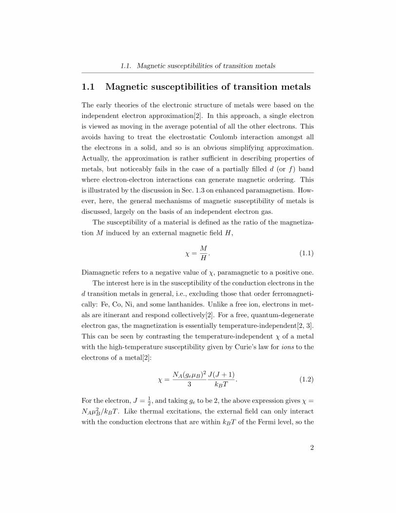
1.1 Magnetic susceptibilities of transition metals
The early theories of the electronic structure of metals were based on the
independent electron approximation[2]. In this approach, a single electron
is viewed as moving in the average potential of all the other electrons. This
avoids having to treat the electrostatic Coulomb interaction amongst all
the electrons in a solid, and so is an obvious simplifying approximation.
Actually, the approximation is rather sufficient in describing properties of
metals, but noticeably fails in the case of a partially filled d (or f) band
where electron-electron interactions can generate magnetic ordering. This
is illustrated by the discussion in Sec. 1.3 on enhanced paramagnetism. How-
ever, here, the general mechanisms of magnetic susceptibility of metals is
discussed, largely on the basis of an independent electron gas.
The susceptibility of a material is defined as the ratio of the magnetiza-
tion M induced by an external magnetic field H,
χ =M
H. (1.1)
Diamagnetic refers to a negative value of χ, paramagnetic to a positive one.
The interest here is in the susceptibility of the conduction electrons in the
d transition metals in general, i.e., excluding those that order ferromagneti-
cally: Fe, Co, Ni, and some lanthanides. Unlike a free ion, electrons in met-
als are itinerant and respond collectively[2]. For a free, quantum-degenerate
electron gas, the magnetization is essentially temperature-independent[2, 3].
This can be seen by contrasting the temperature-independent χ of a metal
with the high-temperature susceptibility given by Curie’s law for ions to the
electrons of a metal[2]:
χ =NA(geµB)2
3
J(J + 1)
kBT. (1.2)
For the electron, J = 12 , and taking ge to be 2, the above expression gives χ =
NAµ2B/kBT . Like thermal excitations, the external field can only interact
with the conduction electrons that are within kBT of the Fermi level, so the
2
1.1. Magnetic susceptibilities of transition metals
fraction of electrons that contribute to χ is[3] T/TF . Scaling the result for χ
by this ratio, the magnetization of the conduction electrons thus follows[3]
M ≈ NAµ2B
kBTFH, (1.3)
which is independent of temperature.
An accurate expression for the susceptibility of the conduction electrons
was given by Pauli (who corectly treated them with Fermi-Dirac statistics)[2,
3], and so is termed the Pauli spin susceptibilty χP , or Pauli paramagnetism.
A simple but useful way to derive it[4] is to neglect the orbital response of
the electrons to the external field (i.e., consider the spin only)[2, 4]. Then,
to lowest order, the effect of the applied field is to shift the relative energy
distribution of electrons with up and down spins[4]. The total energy of
the electrons is now the kinetic energy plus the magnetic contribution of
±µBH[3]. The electrons will adjust such that the chemical potential of the
spin up and spin down electrons will be equal, i.e., the bands will have the
same EF [3, 4]. Because the gyromagnetic ratio of the electron is negative,
there will be a net increase in the density of electron orbitals anti-parallel to
the field, resulting in a moment parallel to the field[3, 4]. If N+(−) denotes
the concentration of electrons with moments parallel(anti-parallel), then the
magnetization density is[2, 3]
M = µB(N+ −N−). (1.4)
In terms of the shifted density of states D(E), the electron concentrations
are given by
N± =
∫
D±(E)f(E)dE, (1.5)
where f(E) is the Fermi function. Since the Fermi energy sets the scale for
the change in D(E), and µBH ∼ 10−4EF (even for Tesla fields) the density
of states can be expanded leading to[2]
N± =1
2
∫
D(E)f(E)dE ± 1
2µBH
∫
D′(E)f(E)dE, (1.6)
3
1.1. Magnetic susceptibilities of transition metals
where D′(E) represents the first derivative. Substituting into Eq. (1.4), the
magnetization density is thus[2]
M = µ2BH
∫
D′(E)f(E)dE, (1.7)
which can be recast as
M = µ2BH
∫
D(E)
(
− ∂f
∂E
)
dE. (1.8)
As T → 0, f(E) approaches an inverted step function at EF [4, 5], and its
derivative is well approximated by the negative of the Dirac delta-function:
−∂f/∂E = δ(E − EF ), which leads to[2, 4, 5]
M = µ2BHD(EF ). (1.9)
By means of Eq. (1.1) the Pauli susceptibility is thus
χP = µ2BD(EF ); (1.10)
i.e., it is linearly proportional to the density of states at the Fermi level.1
The above derivation is made for T ≪ TF — basically, practical temperatures[5]—
and is valid until T ≈ TF ∼ 104 K[2].
In the noble metals, like Cu, Ag, and Au, the Fermi energy lies just
above the d band in the s band; χP is accordingly small in these metals[4].
In fact, in general, χP for most metals is quite small in comparison to the
susceptibility of free ions. For an ion with unpaired spins, the tendency for
spin moment alignment with a field is reduced by thermal disorder (Curie’s
law); while the paramagnetic susceptibility of the conduction electrons is
greatly supressed by the exclusion principle[2]. For instance, [Eq. (1.2)] for
a paramagnetic ion of spin 12 at room temperature, χ ∼ 10−3 emu/mol; while
for typical transition metals [Eq. (1.3)], χP ∼ 10−5 emu/mol, i.e., hundreds
of times smaller[2].
The magnetization of a Curie-law paramagnet follows an inverse-T de-
1The density of states at the Fermi level will be denoted by DF .
4
1.1. Magnetic susceptibilities of transition metals
pendence; while, in contrast, it was stated above that the magnetization of
metals is essentially independent of T . The latter is an oversimplification;
many metals do show a temperature-dependent χP , although often, but not
always, over ranges of absolute T spanning a couple orders of magnitude.
Since the d band is narrow with a higher density of states and DF ∼ kBT
when the Fermi level is in this band, χP is not only larger than for met-
als where EF lies in the s band, but it also leads to a T -dependent χP [4].
The temperature dependence of χP is a consequence of the structure in the
Dd(E), as well as electron interactions (Sec. 1.3).
In addition to χP , there are other sources of magnetism in a transition
metal that arise from the orbital susceptibility of the electrons χorb.2 De-
pending on the metal, this susceptibility may be neglible or considerable in
relation to the spin susceptibility. In the above discussion of χP , only the
spin of the electrons was considered, and the charge was neglected. How-
ever, the external field couples to the orbital motion of the electronic charge
and this gives rise to a diamagnetic response, i.e., M that is antiparallel to
H[2]. For a free electron gas, Landau found[2, 3, 4]
χL = −1
3χP ; (1.11)
termed the Landau diamagnetism.
The energy of these orbital levels can be found only by using a quantum
mechanical approach (as Landau did for the free electron gas); however,
evaluating the orbital motion of electrons in a periodic potential of a crys-
talline lattice, i.e., Bloch electrons, in the presence of the applied field is
quite complicated[2, 4, 6, 7]. The potential can alter the orbital motion of
the electrons, sometimes generating a paramagnetic contribution, and also
sometimes introducing a contribution from spin-orbit (s-o) coupling[6]. Un-
like χP , which is independent of applied field, the orbital effects are second-
order in field. While the above Landau diamagnetism can be considered
appropriate for nearly free electrons like those of the s band, when a realis-
2The paramagnetism arising from the magnetic moments of the nuclei is ∼ 10−3 timessmaller than that from the electrons[3, 9], and is negligible.
5
1.1. Magnetic susceptibilities of transition metals
tic d band structure is considered, the orbital susceptibility may acquire a
paramagnetic contribution if the d band is partially filled. This effect (first
pointed out by Kubo and Obata[8]) can be considered as the itinerant elec-
tron analog of the van Vleck susceptibility of ions[4, 5]: the applied field
causes interband mixing of the electronic states below and above the Fermi
level[4, 9], similar to the mixing of low lying excited states into the ground
state by the applied field in free ions[2, 4]. This contribution, denoted χvv, is
thus greatest when the Fermi level lies in the middle of the d band, as there
are then many states which can be combined by the applied field[7]. As
outlined below, NMR provides one means of separating the contributions of
χvv and χP from the total susceptibility. Another is a magnetomechanical
technique[9]. Such measurements found large values of the orbital param-
agnetism relative to the spin magnetism in metals like V and Nb, and as
expected, the opposite for the metals Pt and Pd[9, 10].
Calculations of χorb have been performed for transition metals by a gen-
eralization of the complicated expressions in combination with calculated
band structures, including the effects of s-o coupling[7, 11]. The latter is a
relativistic correction to the orbital susceptibility. The s-o coupling is gener-
ally regarded as an atomic property, and so it is often assumed that atomic
values largely apply to the solid state. Its importance for the d metals thus
follows that expected from trends in atomic s-o coupling down a group, i.e.,
it is weak in Ni, moderate in Pd, and strongest in Pt[7] as a consequence of
the increasing relativistic motion of electrons with increasing nuclear charge.
In addition to χL and χvv and its s-o contributions, the orbital susceptibility
also includes a diamagnetic contribution χdia from the filled electron levels
of the cores of the ions (or atoms) in the lattice[5, 7, 9, 10, 11]. This dia-
magnetism is analogous to that of the filled electron levels in a paramagnetic
ion, and is termed the Langevin (or Larmor) susceptibility[2, 5]. In many
cases, the diamagnetic and paramagnetic parts of χorb compensate, and χorb
is overall small[7, 10, 11].
In considering the paramagnetism of a metal where the Fermi level lies
in the d band, the total susceptibility is conventionally decomposed into the
6
1.2. Conventional NMR of metals
sum of four major contributions[12], namely
χ(T ) = χs + χd(T ) + χvv + χdia, (1.12)
where χP has been split into individual contributions from the s and d
bands. Only that of the d band explicitly varies with T . The other three
contributions are independent of T , although in some cases χvv can show a
dependence on T [4]. It is emphasized that the above is an approximation
which is valid in the limit of completely independent s and d bands, i.e., in
the limit of vanishing s−d hybridization. In spite of this, it is at least a good
starting point for the discussion of the susceptibility of transition metals.
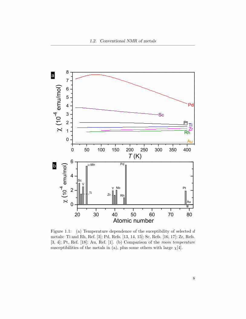
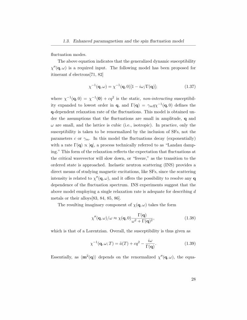
The total susceptibilities of select d metals as a function of temperature are
displayed in Fig. 1.1 showing a representative range of behaviour. In the
group 11 (noble) metals where the d band is completely filled and DF lies
in the sp band, χP is small compared to the diamagnetic contribution and
the overall observed susceptibility is negative[1, 7]. In stark contrast, the
susceptibility of Pd is quite large. As the total contribution from χorb is at
most a few percent, the large paramagnetism is due to the contribution of
the d electrons and makes Pd rather unique among the transition metals.
The origin of this large paramagnetism is discussed in greater detail in Sec.
1.3 below.
1.2 Conventional NMR of metals
As in the study of molecules, conventional NMR has been an invaluable tool
in advancing the knowledge of the magnetic properties of solids. This is
particulary true because it is a technique that can yield information about a
sample on a local, or atomic, level. Two important experimental quantities
measured by NMR are the frequency shift, and the (longitudinal) spin-lattice
relaxation rate. These are outlined below with reference to examples of NMR
in transiton metals.
7
1.2. Conventional NMR of metals
Figure 1.1: (a) Temperature dependence of the suceptibility of selected dmetals: Ti and Rh, Ref. [3]; Pd, Refs. [13, 14, 15]; Sc, Refs. [16, 17]; Zr, Refs.[3, 4]; Pt, Ref. [18]; Au, Ref. [1]. (b) Comparison of the room temperature
susceptibilities of the metals in (a), plus some others with large χ[4].
8
1.2. Conventional NMR of metals
1.2.1 Knight shift
In conventional NMR, application of a static external magnetic field H0
causes the degenerate nuclear magnetic levels of a spin I > 0 nucleus to be
split into (2I+1) magnetic sublevels[2]; this is known as the nuclear Zeeman
splitting. The levels can be designated by the nuclear spin quantum number
mI , with the axis of quantization taken to be along the direction of H0. The
splitting between each sublevel is ∆EmI = γnhH0, where γn is the nuclear
gyromagnetic ratio which is proportional to the nuclear magnetic moment.
Application of an alternating, radio frequency, magnetic field H1 transverse
to H0 results in resonant absorption that is detected to give a spectrum[2].
The allowed transitions occur for ∆mI = ±1, at an angular frequency[20]
hω = ∆EmI = hγnH0. (1.13)
In a metal, the nuclei are found to resonate at frequencies shifted from
Larmor frequency νL (= γnH0) for the free nucleus due to the interaction
with the conduction electrons. This shift was first reported on by W. Knight
and co-workers[22], and so is termed the Knight shift K[5, 12, 19, 20, 21].
It arises from the conduction electron (para)magnetism through the Fermi
contact interaction, i.e., χP [Eq. (1.10)] effectively producing an additional
field at the nucleus that adds to the applied field. This is a quantum me-
chanical interaction, since it originates from two particles being “at the same
place”[5]. As such, this extra field experienced by the nucleus is termed the
contact hyperfine (hf) field, and it is usually an order of magnitude larger
than the chemical shifts observed in metal salts[20].
The Hamiltonian for the Fermi contact interaction for nuclear spin Ii
with electron spin Sj reads
He−n =8π
3γeγnh
2∑
i,j
Ii · Sjδ(rij), (1.14)
where γe is the electronic gyromagnetic ratio, and rij are the position co-
ordinates of the nucleus and electron. Since it is only electrons of s symmetry
9
1.2. Conventional NMR of metals
that have a finite probability of being found at the nucleus (i.e., they have
no node at the nucleus), the hyperfine field from the contact interaction
involves the square of the s-wavefunction at the nucleus ψs(0) normalized
to the atomic volume, averaged over electrons on the Fermi surface (and so
this interaction is intrinsically isotropic);
K =8π
3〈|ψs(0)|2〉FχP . (1.15)
For this result, the Knight shift is defined as a fractional shift, K ≡ ∆H/H0;
where ∆H is the extra field at the nucleus, and the dependence on H0 is
thus normalized out. In terms of experimentally measured frequencies,
K =ν
ν0− 1. (1.16)
Here ν is the resonance frequency in the metal, and ν0 is the reference
frequency relative to which K is determined. It is therefore important that
the reference be nonmetallic and nonmagnetic. Usually, diamagnetic ionic
salts (or solutions of them) of the nucleus of interest are used; ν0 is then
typically very close to νL, differing by the chemical shift which is small
in comparison to shifts arising from the paramagnetic contributions of the
conduction electrons. Values of K are typically expressed in per cent or
parts per million (ppm), depending on their magnitude.
Eq. (1.15) can be re-expressed in terms of a constant times the suscep-
tibility
K = Ahfχi. (1.17)
The term Ahf is the hyperfine coupling constant that represents the addi-
tional hf field at the nucleus. The above equation indicates that a knowledge
of both the electronic magnetic susceptibility and the extent of its coupling
to the nucleus is required to quantitatively understand the Knight shifts in
metals. Often Ahf is estimated from the hf splitting measured in the free
atom, but this is at best a first approximation. In principle, χ can be mea-
sured by magnetometry, e.g., using a SQUID, or estimated from values of
the electronic contribution to the specific heat; however, such measurements
10
1.2. Conventional NMR of metals
give the macroscopic, bulk susceptibility which contains other contributions
beside χP . The attractiveness of the NMR technique is that it can probe
samples at the microscopic level, and reveal the differing hf fields experienced
by various nuclei in the material.
In Eq. (1.17), the Pauli susceptibility has been replaced by χi, since
in the study of transition metals, the measured shift is decomposed into
contributions from the various terms in Eq. (1.12); each with a distinct
coupling constant. As previously mentioned, the diamagnetic component is
small in comparison to the others, and often assumed to be of equivalent
magnitude to the atomic chemical shift of the diamagnetic reference salt
(although deviations are not uncommon)[5]. Equations (1.12) and (1.17)
indicate that for metals with filled d bands like the simple metals, K will be
essentially temperature-independent. In metals with near half-filled d bands
(e.g., V and Nb), the orbital paramagnetic susceptibility is large and gives
the dominant contribution to the observed shift[12, 21]. This shift may be
T -dependent with ∂K(T )/∂χ(T ) usually positive[12]. In these cases, the
contributions from χs and χd largely cancel[12, 23]. This arises from the
mechanism by which χd affects K, and is crucial for metals with nearly
filled d bands (e.g., Pt and Pd); the shifts are observed to be strongly T -
dependent and negative[12, 21].
The d wavefunctions vanish at the nucleus, so their effect on the spin
density is due to the mechanism of “core-polarization”[12], whereby the spin
polarization of the unfilled d shells is mixed into the core s electron wave-
functions. An analogous situation is encountered for hf fields of atoms or
paramagnetic ions, i.e., a configuration interaction that mixes excited states
into the ground state[12, 21, 24, 25]. This indirect polarization takes place
through an electron-exchange interaction like that occurring between elec-
trons in the d band that is responsible for the enhanced susceptibility of Pd
discussed below. This is like saying that s electrons with spin parallel to the
polarized d electrons experience a reduced electrostatic repulsion due to the
Pauli principle and are overall less repelled by one another than by electrons
with spins antiparallel[24]. The result is differing spatial distributions of the
core electrons of opposite spin; s electrons with spins parallel to the d elec-
11
1.2. Conventional NMR of metals
trons are attracted away from the nucleus, indirectly giving rise to a negative
spin density (i.e., antiparallel to the d polarization) at the origin producing
a negative contact hf coupling[21, 24]. The small number of valence (i.e.,
non-core) s electrons are polarized indirectly by the d spins also, but give
a positive contribution at the origin[24]. The contribution from χs of the
valence electrons is therefore considered the direct contact interaction, and
yields a positive shift. As DsF is small (and practically T -independent), the
contribution from χd(T ) can cancel or exceed the direct contribution[12];
this is especially true in transition metals with large susceptibilities, like Pt
and Pd.
The dipolar coupling between the electron and nuclear spins can add
to the field at the nucleus, and hence to the shift. The contribution from
the coupling of the nuclear moment to the electron spin of a d or p orbital
electron can thus be anisotropic and depends on the direction of H0 relative
to the crystalline axes[12, 20, 21]. For cubic metals, these couplings gives
no contribution, but may be non-zero at sites where the symmetry of the
spin density is reduced. As conventional NMR is frequently performed on
powdered samples rather than single crystals, any anisotropy of the elec-
tronic dipolar-nuclear coupling can give rise to structure of the resonance
line. However, the dipolar coupling field is normally an order of magnitude
smaller than the contact or core-polarization contributions, and generally
produces a broadening of the resonance[20, 21].
The temperature dependence of K from 195Pt NMR was reported by
Clogston et al.[26]. The measured shifts were used in combination with
the measured total χ of Pt to separate the different contributions in Eq.
(1.12). They observed a linear dependence of K with χ (from room T
and below) and displayed this in a K − χ plot (or “Jaccarino-Clogston”
plot) in which T is an implicit parameter[12]. The shifts3 were found to be
negative and ∼ −3% in the T range investigated. The analysis thus involved
3These early metal NMR measurements were performed in field-swept mode, i.e., thefield was varied with the transverse radio-frequency field held constant. The K valuescorrespond to Eq. (1.16) with the frequencies replaced by the resonant fields for the metalsample and the reference.
12
1.2. Conventional NMR of metals
estimations of χs and χdia. The s electrons were treated as free electron-like,
and s − d (and s − s) exchange interactions were neglected. Accordingly,
χs was taken to be small and T -independent; χdia was estimated on the
basis of the susceptibilities of Pt salts; χvv was determined by a method
of extrapolation of the data on the K − χ plot, and found to contribute
∼ 15 of the observed K, but positive in magnitude (and not dependent on
T ). Overall, the negative χdia together with the small, positive χs nearly
cancel the contribution from χvv, an indication that the observed shifts,
with ∂K(T )/∂χ(T ) < 0, must be dominated by the d spins. This was taken
as clear support for the model of polarization of the core s electrons by
the d spins as the mechanism for the large, negative, T -dependent shifts
in metals with nearly filled d bands[12]. In a later NMR study of Pt a
K − χ plot analysis was performed for temperatures extending to ∼ 1300
K[27] and the results were in agreement with the earlier report[26], especially
with respect to the cancellation of the diamagnetic and orbital paramagnetic
contributions, reinforcing the importance of the d electrons.
Subsequently, Seitchik, Gossard, and Jaccarino performed a similar study
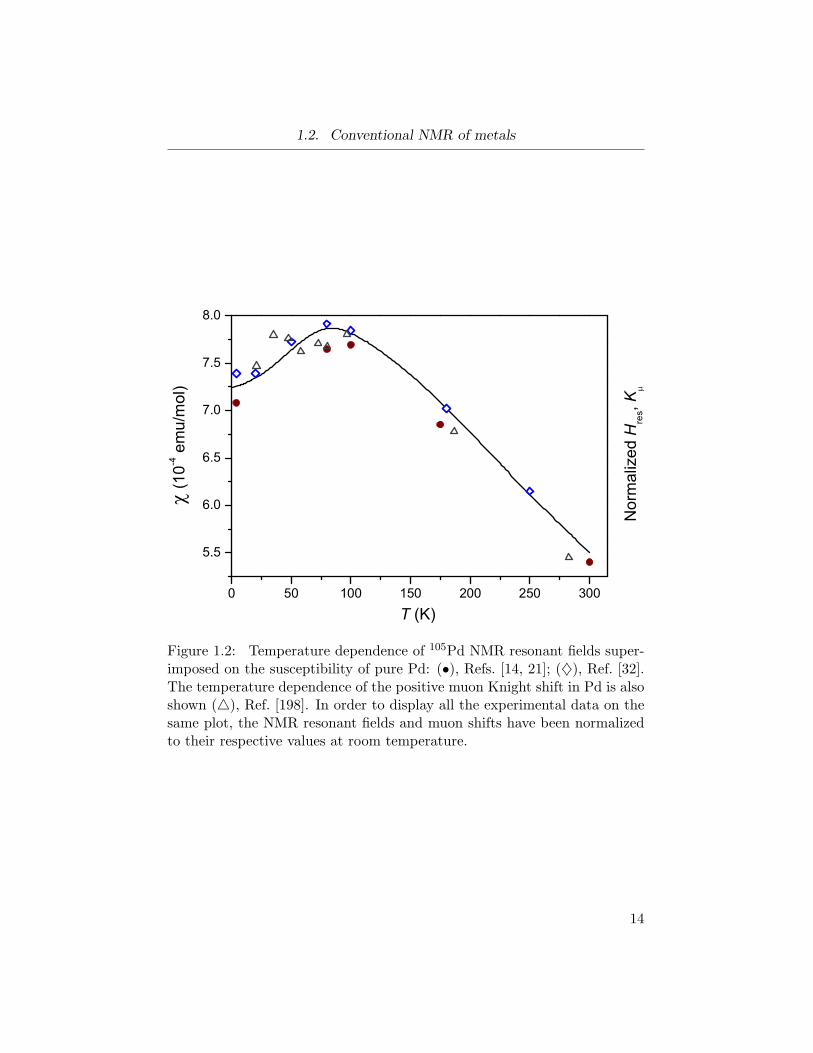
of Pd metal, the first observation of 105Pd NMR[14]. As in Pt, T -dependent,
negative Knight shifts were observed that scaled linearly with the suscepti-
bility, including its maximum at around 85 K (see Fig. 1.2). The Knight shift
was observed to vary between -3% to -4% over the T range; however, unlike
in the analysis for Pt, the nuclear moment of 105Pd was not known very ac-
curately at the time, and so the zero of shift could not be determined with
great certainty. This precluded the graphical determination of χvv from the
K−χ plot. Instead, it was estimated to be ∼ 25×10−6 emu/mol, along with
χs (6 × 10⁻⁶ emu/mol) and χdia (−25 × 10−6 emu/mol). Their estimated
value of the orbital susceptibility is similar to the values later reported[7, 9];
however, more recent fully relativistic calculations[11] put χvv ∼ 40 × 10−6
emu/mol.
The sum of the above three estimates amount to just ∼ 1% of the total
χ of Pd. Nonetheless, χs and χvv were determined to give a contribution
of +0.36% each to the observed K, independent of T . Thus, analogous to
Pt, it was concluded that the enhanced d spin contribution dominates the
13
1.2. Conventional NMR of metals
Figure 1.2: Temperature dependence of 105Pd NMR resonant fields super-imposed on the susceptibility of pure Pd: (•), Refs. [14, 21]; (♦), Ref. [32].The temperature dependence of the positive muon Knight shift in Pd is alsoshown (△), Ref. [198]. In order to display all the experimental data on thesame plot, the NMR resonant fields and muon shifts have been normalizedto their respective values at room temperature.
14
1.2. Conventional NMR of metals
observed Knight shifts through core-polarization and is responsible for the
temperature dependence of K. Although χs is a tiny fraction of the total
χ, Ashf was evaluated to be an order of magnitude larger than Ad
hf , so the
direct contact contribution is not entirely negligible.
More recently, Krieger and Voitlander performed a calculation of K for
Pd[28]. They evaluated the contribution from all s, p, and d levels and in-
deed found that polarization of core electrons gives the majority, negative
contribution, as the direct contact contribution is +0.18%. Their total K
(for T = 0) is -3.34%, which is adequate compared with the 4 K experimental
result of -4.1(5)%[21] considering the uncertainty in the zero of shift. How-
ever, no (positive) orbital contribution to K was included in the calculations
of Ref. [28], which only reduces the agreement with experiment.
The hyperfine field, as a low energy property, is a quantity that provides
a strict test for first-principles calculations. Generally, calculated values are
smaller than experimental ones. The dominance of the core-polarization
contribution in strong paramagnets is also found in magnetically ordered
metals, like Fe. Reducing the discrepancy with experiment requires treat-
ment of this contribution beyond what is typically achievable with common
ab initio methods[11, 29, 30]. Additionally, s− d hybridization is increased
in the 4d and 5d metals, which can make a contribution irrespective of the
exchange coupling. For instance, Terakura et al. pointed out that the direct
contact contribution in Pd should be both larger and negative (∼ −1%) due
to s− d hybridization[31].
Takigawa and Yasuoka also carried out measurements of the resonant
fields in metallic Pd, but for more T points[32] (select values from their
measurements are also shown in Fig. 1.2). They report results very simi-
lar to those of Seitchik et al. upon decomposing the shift into the various
contributions. Just as in the earlier study, they considered the dominant
contribution to be from the core-polarization from d electrons and allowed
for this to be the only T -dependent term. Using values of the hyperfine
fields from first-principles band structure calculations[33], they estimated
the direct contribution to be +0.12%, but used a very similar value for the
diamagnetic contribution and the same (+0.36%) orbital contribution as
15
1.2. Conventional NMR of metals
Seitchik et al.[14]. From the T -dependence of their shifts, these authors[32]
determined a comparable d spin (i.e., core-polarization) hf coupling, but a
smaller direct coupling than in Ref. [14]; however, the coupling constants
extracted agree with the earlier report that Ashf is an order of magnitude
larger than Adhf .
In considering more appropriate values for the 105Pd reference frequency,
van der Klink and Brom[5] performed an analysis of the contributions to K
that leads to a total shift of -3.44%. They employ a direct contribution
based on requiring Ashf be of similar order to that of Pt, and obtain +0.62%
with an orbital contribution of +0.36%. The latter value is the same as in
the earlier two studies[14, 32], but the direct part required is a factor of
2 larger. Although this is the most modern analysis, estimations based on
comparison to values for Pt are questionable; a larger direct contribution is
expected for increased s− d hybridization.
Given that there is really only “one” (i.e., total) χ, it is apparent that any
such decomposition of experimental K’s requires considerable estimation by
means of calculation or comparison to other metals. However, a rather clear
consensus on the sign and order of magnitude for the three contributions (s,
d, and orbital) is broadly found.
NMR has also been extensively applied to the study of metallic alloys.
In particular, those formed from a magnetic impurity in an otherwise non-
magnetically ordered host (e.g., CuFe) have been of interest with respect
to the mechanism(s) and degree of polarization of the host by the magnetic
moment of the impurities[34]. These systems are not discussed in detail
here, but one result from the NMR of such alloys is worth mentioning in
regard to adventitious contamination of a metal sample by dilute, mag-
netic impurities: K of the host nuclei is not affected by the presence of the
magnetic impurities[26, 35]; the resonance line is instead broadened pro-
portional to the impurity susceptibility. This also holds for a host with an
enhanced susceptibility, like Pt, as evidenced from 195Pt NMR in samples
alloyed with dilute (< 0.1 at.%) Co; the shift was not found to vary, while
the linewidth showed a linear increase with increasing Co concentration[36].
In such (dilute) systems, the linewidth of the host resonance was calculated
16
1.2. Conventional NMR of metals
to approach a Lorentzian lineshape[37], which was indeed observed in the
NMR of CuMn[35] and PtCo[36] alloys.
1.2.2 Spin-lattice relaxation and the Korringa relation
In order to discuss the spin-lattice relaxation, the generalized magnetic sus-
ceptibility must be recalled:
χ(q, ω) = χ′(q, ω) + iχ′′(q, ω), (1.18)
where χ′(q, ω) and χ′′(q, ω) are the real and imaginary components, respec-
tively. χ(q, ω) defines the response of the system to a generalized exciting
field that varies periodically with angular frequency ω and with a spatially
periodic fluctuation of wavevector q (|q| = 2π/λi). The uniform, static
limit of the real component is identified with the Pauli susceptibility (of
non-interacting electrons), cf. Eq. (1.10),
χ′(0, 0) =1
2γ2
e h2DF . (1.19)
As discussed above, the Knight shift is proportional to the real component,
while it is the imaginary (dissipative) component that is important for the
spin-lattice relaxation rate.
For transition metals, the Fermi contact interaction produces a large hf
field at the nucleus, and so the spin-lattice relaxation process occurs predom-
inantly through this interaction. Specifically, the longitudinal relaxation of
the nuclear magnetization (in non-magnetically ordered metals) that arises
from transverse fluctuations associated with Eq. (1.14). The general mech-
anism is that of mutual spin-flip scattering of an electron off the nucleus. A
Bloch s electron in the initial state of wave vector k with spin orientation
se undergoes a transition to the final state k′, s′e, and the nucleus simulta-
neously makes a transition from state mI to m′I [19, 20]. The nucleus gives
the electron an energy small in comparison with kBT , so only electrons near
EF with empty states nearby in energy can participate in the relaxation[20].
The relaxation rate thus depends on temperature through the width of the
17
1.2. Conventional NMR of metals
“tail” of the Fermi distribution[20]. The number of available states increases
as the width with increasing T , so the rate is directly proportional to T . The
observation of a spin relaxation linear with temperature is one important
method of establishing that a material (i.e., solid) is metallic[38].
The transverse fluctuations on which the relaxation rate depend are given
by an integral over wavevectors of the imaginary part of the dynamical
susceptibility[12, 39, 40],
1
T1=
32
9γ2
n〈|ψs(0)|2〉2FkBT1
ωL
∫
q2χ′′(q, ωL)dq. (1.20)
In the above expression, the frequency of interest is specifically the nuclear
Larmor frequency, which corresponds to the low frequency limit for typical
electronic magnetic fluctuations. The integral can be evaluated for a free
electron gas:1
ωL
∫
q2χ′′(q, ωL)dq = 2π3γ2e h
3D2F . (1.21)
Substitution of this result into Eq. (1.20) results in
1
T1T=
64
9π3h3kBγ
2eγ
2n〈|ψs(0)|2〉2FD2
F . (1.22)
Since the relaxation depends on the electron-nuclear contact interaction,
〈|ψs(0)2|〉F is the same as that appearing in Eq. (1.15),
〈|ψs(0)2|〉2F =9
64π2
K2
χ2P
. (1.23)
Inserting this quantity into Eq. (1.22) gives
1
T1T= K2kBπh
3γ2eγ
2n
D2F
χ2P
. (1.24)
Using χP given by χ′(0, 0) from Eq. (1.19) yields a very useful relation in
NMR:
T1T =h
4πkBK2
(
γe
γn
)2
. (1.25)
The above expression shows that the relaxation rate due to the conduction
18
1.2. Conventional NMR of metals
electrons is inversely proportional to the square of the shift, or by exten-
sion [Eq. (1.17)], to the square of the hf coupling. Eq. (1.25) is known as
the Korringa relation[5, 19, 20, 21, 41], which upon re-arrangement can be
expressed as a dimensionless ratio
K =T1TK
2
S0, (1.26)
where S0 is a single constant into which all the constants in Eq. (1.25) have
been incorporated, and is specific to a given nucleus (through γn).
The Korringa relation provides a convenient way to estimate the shift
given a measurement of the relaxation rate, or vice-versa[20]; however, it is
emphasized that the relation is strictly valid for non-interacting electrons.
In such an ideal case the ratio K as defined in Eq. (1.26) is unity, but for
real metals deviations are observed. These are often attributed to the break-
down of the relation due to neglect of electron-electron interactions on the
dynamic susceptibility[5], although only the electron-nuclear mechanism is
considered, so the neglect of other relaxation processes may also contribute
to deviations[20]. Values of K different from 1 are found even for the “sim-
ple” metals such as the alkalis or the noble metals[5, 20]. For instance, K is
1.6 for Li, and 1.9 for Cu[21]. For metals with strong electronic correlations,
significant deviations from ideality are found; e.g., for Pd K = 9.4[21]. In
this regard, K is frequently used as a phenomenological measure of the ten-
dency toward magnetic ordering. As defined in Eq. (1.26), K > 1 is taken to
be indicative of ferromagnetic correlations, and K < 1 of anti-ferromagnetic
correlations.4
An additional aspect of the spin-lattice relaxation rate of the transition
metals (those with EF in the d band) that must be taken into account is
the orbital degeneracy factor (viz. eg and t2g levels)[12, 42]. This factor,
denoted Fd, represents a reduction, or “inhibition,” of the relaxation due to
4Often the inverse of Eq. (1.26) is used, in which case the type of ordering attributedto the magnitude of K is reversed.
19
1.2. Conventional NMR of metals
the core polarization by an amount
Fd =1
3f2 +
1
2(1 − f)2, (1.27)
where, here, f is the fractional character of the triply degenerate orbital
at EF ; Fd correspondingly varies from 0.2 to 0.5. For Pd, calculations[33]
give f = 0.78. A similar dependence on the atomic orbital admixture also
applies to the orbital or dipolar contributions to the relaxation rate[42, 43].
The conduction electron mechanism is generally taken to be the dominant
source of nuclear spin relaxation with the orbital contribution playing a
less important role (except for metals with a half-filled band where it can be
significant); the dipolar contribution is most generally the least effective[43].
Thus, for the case of T−11 dominated by d electrons the Korringa relation
is more specifically written as,
(T1T )−1d =
4πkB
h
(
γn
γe
)2
K2cpFdK(α0). (1.28)
Here the inverse of the enhancement K−1 has been replaced by the term
K(α0). In this way the Korringa factor is used to quantify the degree of
electron-electron interactions in a metal. This was originally considered by
Moriya[39] for metals where d electron interactions give rise to large suscep-
tibility enhancements (citing Pd as a specific example), but can equally be
applied to simple metals since even these metals show deviations from ideal-
ity (K = 1)[44, 45]. The quantity α0 thus reflects the degree of susceptibility
enhancement (it can be taken to be equivalent to the Stoner parameter I0,
discussed in Sec. 1.3 below) and varies from 0 to 1[39, 44, 45]. According
to the present definition of K, α0 → 1 as the enhancement increases. This
theory is strictly valid for the ground state, i.e., for T ≃ 0. However, care
must be taken when applying this approach to real systems, since it was later
shown that crystallographic disorder or non-magnetic impurities can alter K(typically be increasing T−1
1 ), thus making definitive conclusions about the
degree of enhancement difficult[46, 47]. Additionally, all other mechanisms
of relaxation (e.g., orbital) must also be taken into account before drawing
20
1.3. Enhanced paramagnetism and the spin fluctuation model
any conclusions about electron interactions from the Korringa ratio[48].
1.3 Enhanced paramagnetism and the spin
fluctuation model
Referring to Fig. 1.1, it is seen that Pd has a very large and temperature-
dependent magnetic susceptibility in contrast to the other metals. Note
the temperature-independent and overall diamagnetic susceptibility of Au,
typical of the noble metals. Pd has the largest χ of any transition metal
that does not order magnetically in the pure, bulk state. The peculiar max-
imum or “knee” at T ≈ 85 K prompted the authors of one of the earliest
measurements of its susceptibility to state that their results “proved to be
much more interesting than was expected”[49]. As seen in Fig. 1.1(a), Sc
also exhibits such a maximum for T ≈ 30 K. The susceptibilities of these
two metals and that of Pt are characteristic of what is known as exchange-
enhanced paramagnetism. Fig. 1.1(b) shows that Pd, followed by Sc, are
the most exchange-enhanced of the nonmagnetic d-metals[50] (α-Mn orders
antiferromagnetically at low T ); however, there are also many metallic alloys
and compounds that fall into this class of magnetic materials (examples are
given below). Sc possess a hexagonal close-packed (hcp) crystal structure
giving rise to anisotropy of its susceptibility, i.e., χc 6= χa[16, 17], which in
this case arises from the orbital motion of the electrons caused by the s-o
coupling[51] (the data in Fig. 1.1 is for a polycrystalline sample).5 The crys-
tal structures of alloys/compounds are also often complex. By comparison,
Pd crystallizes in the face-centred cubic (fcc) lattice structure, which greatly
simplifies matters.
It is emphasized that neither Pd, nor Sc, in their pure bulk states, show
any type of magnetic ordering at any temperature. This is in contrast to the
well-known magnetic 3d metals[1]: Fe, Co, and Ni that order ferromagneti-
cally below their respective Curie temperatures TC ; Mn and Cr order anti-
5Sc is also like V and Nb in regards to the orbital term dominating, thus producing ananisotropic K[23].
21
1.3. Enhanced paramagnetism and the spin fluctuation model
ferromagnetically below their respective Neel temperatures TN .6 Nonethe-
less, on account of their high susceptibilities, an intriguing characteristic of
many enhanced paramagnetic materials is the ease with which they may
be promoted to order magnetically via some external parameter, such as
the application of an external magnetic field, doping with small amounts of
magnetic impurities, or a change in lattice constant. This imparts a degree
of potentially useful “tunability” to their magnetic behaviour. For the par-
ticular case of Pd, the ease of inducing ferromagnetic ordering has been well
documented over many decades. Thus, the ground state of pure Pd can be
considered proximal to a ferromagnetic instability, i.e., it is often described
as a nearly ferromagnetic metal. Similarly, this statement holds for Sc and
to a lesser extent for Pt. Strong paramagnets such as these require treat-
ment analogous to systems that show magnetic ordering; a summary of this
theory is now given.
Historically, the development of the theory of metallic magnetism fo-
cussed on the 3d ferromagnets with the emphasis on calculating their TC
values from first principles[1]. In contrast to isolated moments in insu-
lators (where the Heisenberg model[2, 4] works well), a model based on
well-defined, localized moments fails for metals. This is because the elec-
trons responsible for the magnetism are the intinerant, conduction electrons
that arise from the strong hybridization between neighbouring atoms in a
metal, i.e., the band structure[1]. One of the earliest attempts to incorpo-
rate features of the band structure was a theory proposed by Stoner[53]. As
discussed below, this theory is not correct at finite T , but has merits for
understanding the T = 0 magnetic properties of metals and introduced a
highly useful concept for discussing exchange enhancement.
To start, the susceptibility at T = 0 is considered. Eq. (1.10) shows
that χP is directly proportional to DF . By performing a detailed band-
structure calculation, one can evaluate DF and thus obtain a value of χP .
6The heavier lanthanides, Gd–Tm, also undergo transitions to magnetically orderedstates. A coupling between the highly localized, unpaired 4f electrons mediated by thespd conduction electrons is responsible for the magnetism of these elements[52], and isequivalent to the mechanism of magnetic ordering in many dilute alloys.
22
1.3. Enhanced paramagnetism and the spin fluctuation model
For metals like Pd, such a computation will yield a susceptibility that is
too small in comparison with that measured experimentally for T → 0.
The simplest phenomenological approach is to assume the presence of a
molecular exchange field, denoted by the positive constant I0[1, 54]. This
is a hypothesized internal interaction that acts like an effective magnetic
field that tends to align the spins parallel to each other[3]; in other words,
it increases the spin polarization. So, in the presence of an applied field H0,
the magnetization will follow
M = χ0(H0 + I0M), (1.29)
where χ0 is the susceptibility in the absence of the exchange, i.e., the non-
interacting susceptibility[54]. The exchange field can thus be seen as a source
of positive feedback, that for large enough I0χ0, can induce a spontaneous
magnetic polarization even in the absence of an applied field[54]. Ultimately,
the exchange interaction has its origin in the repulsion due to the Coulomb
interaction (spin-independent) together with the Pauli exclusion principle
(spin-dependent)[2, 4, 54].
At this simplest level of an intraatomic exchange interaction, the suscep-
tibility can be calculated by what is known as the random-phase approxima-
tion (RPA)[2, 55], leading to the expression for the enhanced susceptibility[56],
χ(q, ω) =χ0(q, ω)
1 − Iχ0(q, ω). (1.30)
The term I in the denominator above is known as the Stoner parameter; it
is given by the product I0DF , and defines the Stoner enhancement factor,
S = (1 − I)−1, (1.31)
Thus, in the “static” limit (q → 0, ω → 0), the interacting susceptibility is
that of the Pauli susceptibility [Eq. (1.10)] enhanced by the factor S, i.e.,
χP = Sχ0[1, 4, 56].
Additionally, Eq. (1.31) further provides a quite general condition for
23
1.3. Enhanced paramagnetism and the spin fluctuation model
characterizing the proximity to a magnetic instability; namely, as I → 1,
S → ∞, or alternatively, χ → ∞ signaling the onset of ordering. I ≥ 1 is
thus known as the Stoner criterion[1, 4]. In this regard, Stoner’s criterion is
the simplest condition for a magnetic instability. It is only concerned with
the value of the DOS directly at EF , thus neglecting the structure of the rest
of the DOS; and it is for T = 0, so any possibile effect of finite temperature
on the DOS is also neglected[57].
For Pd, the susceptibility enhancement over that from band structure
calculations[58, 59] usually leads to S ∼ 9 (I ≃ 0.9).7 The Pauli sus-
ceptibility directly depends on DF , and so provides a strong test for such
calculations[60]. This is very true for Pd as EF lies in a region at the top
of the d band where the density of states (DOS) is a rapidly decreasing
function of energy. EF lies just above a sharp peak in the DOS (∼ 25
meV)[58, 59, 60, 61, 62]. DF is accordingly high and very sensitive to the
position of EF [63]. Considering the transition metals, the parameter I for
Pd is only exceeded by those of the 3d ferromagnets and Sc[1, 63]. Indeed,
the fcc band structure is shared by the ferromagnet Ni; however, the key
difference is that in the paramagnetic state EF of Ni lies even closer to the
sharp peak at the top of the band[1].
From theory, the enhancement of the static susceptibility of Pd is strongest
around q ∼ 0 and ω ∼ 0, and decreases quickly with increasing q (with a
Lorentzian form) or ω toward χ0[56, 64, 65, 66]. This is the typical be-
haviour for a ferromagnet. In contrast, antiferromagnetic order is charac-
terized by enhancements at a finite wavevector Q 6= 0[1]; see e.g., Refs.
[51, 65, 66, 67, 68]. I0 is found to have a weak dependence on q, and is
regarded as a local atomic property[1, 63] (and typically taken temperature-
independent). This means the susceptibility is uniformly enhanced[1].
While the “Stoner model” of intinerant electron magnetism[69] in com-
bination with ab initio band structure calculations is quite good for the
ground state (i.e., T = 0); problems are encountered in the application
to finite temperatures[70]. Most notably, the model fails to correctly pre-
dict the transition temperature[1, 71]. For example, the Stoner model pre-
7The more precise values commonly employed for Pd are S = 9.4 or I ≃ 0.89.
24
1.3. Enhanced paramagnetism and the spin fluctuation model
dicts TC values for the 3d ferromagnets that are at least four times larger
than experiment[70]. This is because the disapperance of the static, or-
dered magnetic moments must occur from single particle excitations (spin-
flips) requiring too high an energy ∼ TF [1]. Additionally, the model fails to
adequately describe the Curie-Weiss (CW) behaviour of the susceptibility
frequently observed above the transition temperature; while in the ordered
state, it also does not properly describe the temperature dependence of the
magnetization[71].
Eventually the viewpoint shifted to a focus on collective excitations;
Doniach and Engelsberg showed that such collective modes make corrections
to the energy calculated in the single-particle Stoner (RPA) model when
the exchange enhancement is large[72]. Known as spin fluctuations, they
represent long wavelength, low energy, collective excitations of enhanced
spin density. The characteristic energy is thus reduced by the low energy
of the spin fluctuations as compared to the single-particle excitations (by a
factor S)[72, 73], leading to a renormalization of the finite T susceptibility
and other thermodynamic properties[72, 73]. In particular, better agreement
with experiment is obtained for TC by treating the transition as fluctuation-
driven, and the CW behaviour at high T is also correctly predicted[74, 75].
The spin fluctuations are also known to inhibit Bardeen-Cooper-Schrieffer
(BCS) type superconductivity[76], and are invoked to explain the absence
of superconductivity in elements such as Pd and Sc in their equilibrium
states[77].
With time, an increasing number of structurally ordered alloys were dis-
covered that exhibit very large enhancement factors, e.g., TiBe2 for which
S ∼ 60[67]. Other well-known examples include Ni3Al (and the related
Ni3Ga), ZrZn2, Sc3In, MnSi, and (Sc,Y,Lu)Co2. Several of these systems
order ferromagnetically, but the TCs are rather low (often of the order of
tens of Kelvin); while those that do not order are clearly strongly enhanced
paramagnets, i.e., nearly ferromagnetic. All are metallic, and the intinerant
electrons are responsible for the magnetic properties. In the paramagnetic
state, χ often exhibits an initial quadratic temperature dependence at low
temperature; while at higher temperatures, the susceptibilities are univer-
25
1.3. Enhanced paramagnetism and the spin fluctuation model
sally seen to transition to a CW behaviour that is observable over a wide T
range[71, 78]. Moreover, for those systems that do order, the effective mag-
netic moment µeff obtained from the Curie constant is always larger than
the saturated moment µsat obtained below TC [71, 78]. The term “weak” (or
unsaturated) ferromagnet is used to describe these materials. The Heisen-
berg local moment description is invalidated by the ratio µeff/µsat ≫ 1;
while again, the high characteristic energy scale of the Stoner model makes
it inappropriate[71, 78]. From the 1970s onward, the importance of spin
density fluctuations was becoming clear, and increasing efforts were made
to self-consistently incorporate spin fluctuation (SF) corrections to the RPA
ground state for intinerant electron magnets. Such a theoretical framework
was notably advanced by Moriya and co-workers[71], and Lonzarich and co-
workers[54, 78]. The basic notions of the model are sketched below[79, 80]
(essentially following the formulation of Ref. [54]).
Spin fluctuation effects can be incorporated into the equation for magne-
tization by means of the Ginzburg-Landau framework of phase transitions[81].
In this approach the free energy F is expanded as a power series of an or-
der parameter (that may fluctuate about a mean value). This formalism
is strictly valid near the phase transition. For the case of a transition to a
magnetically ordered state, F is expanded in terms of the magnetization M,
F(M) = F0 +a
2M2 +
b
4M4 +
g
6M6 + · · · . (1.32)
The term F0 represents the free energy of the non-interacting system. The
magnetic equation of state in the limit of T → 0 takes the form,
H =∂F(M)
∂M= aM + bM3 + gM5 − c∇2M. (1.33)
The expansion (Landau) coefficients a, b, c, and g are taken to be inde-
pendent of M in the case of weak ferromagnets/enhanced paramagnets. The
coefficient a represents the inverse of the enhanced susceptibility from the
Stoner (RPA) model, i.e., in the absence of the fluctuations: a = (χ−10 −I0).8
8This means that a is technically T -dependent through the (Stoner) single-particle
26
1.3. Enhanced paramagnetism and the spin fluctuation model
In the paramagnetic state, a is postive; while it changes to negative in the
ferromagnetic state. The coefficient b may be of either sign. In the case that
it is positive, the higher-order term (with coefficient g) is often neglected as
this term is small for weak magnets; however, in the case of negative b this
term must be retained. The term involving the coefficient c represents the
spatial gradient of the magnetization. It is added to take into account spatial
variations of the fluctuations, and is thus related to the q dependence of the
susceptibility. In essence, the fluctuations are assumed to vary in real space
on a scale longer than the electron interactions; this lowest-order gradient
term is introduced to account for the non-locality. The sign of c is positive in
the case of ferromagnetism, and negative in the case of antiferromagnetism.
The temperature dependence of the magnetic equation of state is taken
to arise from the thermally-induced spin fluctuations. They can be viewed as
introducing a random magnetization of zero mean to each term on the right-
hand side of Eq. (1.33). The terms non-linear in M generate corrections
due to the added magnetization. The effect of the SFs is thus to impart a
temperature dependence to the susceptibility, i.e., a renormalization of the
T = 0 coefficients[74]:
a→ a(T ) = (χ−10 − I0) +
5
3b〈m2〉 +
35
9g〈m2〉2, (1.34)
and
b→ b(T ) = b+14
3g〈m2〉. (1.35)
The quantity 〈m2〉 ≡ ξ2 represents the sum contribution from the thermal
variance of the Fourier components of the spin density fluctuation, ξ2 =∑
q〈m2(q)〉; 〈m2(q)〉 is calculated from
〈m2(q)〉 =2
π
∫
∞
0Nωχ
′′(q, ω)dω, (1.36)
where Nω is the Bose function. The coefficient b is identified as the mode-
mode coupling parameter which describes the coupling amongst the spin
excitations; due to the high energy involved, this dependence is typically ignored.
27
1.3. Enhanced paramagnetism and the spin fluctuation model
fluctuation modes.
The above equation indicates that the generalized dynamic susceptibility
χ′′(q, ω) is a required input. The following model has been proposed for
itinerant d electrons[71, 82]
χ−1(q, ω) = χ−1(q, 0)[1 − iω/Γ(q)]; (1.37)
where χ−1(q, 0) = χ−1(0) + cq2 is the static, non-interacting susceptibil-
ity expanded to lowest order in q, and Γ(q) = γmqχ−1(q, 0) defines the
q-dependent relaxation rate of the fluctuations. This model is obtained un-
der the assumptions that the fluctuations are small in amplitude, q and
ω are small, and the lattice is cubic (i.e., isotropic). In practice, only the
susceptibility is taken to be renormalized by the inclusion of SFs, not the
parameters c or γm. In this model the fluctuations decay (exponentially)
with a rate Γ(q) ∝ |q|, a process technically referred to as “Landau damp-
ing.” This form of the relaxation reflects the expectation that fluctuations at
the critical wavevector will slow down, or “freeze,” as the transition to the
ordered state is approached. Inelastic neutron scattering (INS) provides a
direct means of studying magnetic excitations, like SFs, since the scattering
intensity is related to χ′′(q, ω), and it offers the possibility to resolve any q
dependence of the fluctuation spectrum. INS experiments suggest that the
above model employing a single relaxation rate is adequate for describing d
metals or their alloys[83, 84, 85, 86].
The resulting imaginary component of χ(q, ω) takes the form
χ′′(q, ω)/ω ≈ χ(q, 0)Γ(q)
ω2 + Γ(q)2, (1.38)
which is that of a Lorentzian. Overall, the susceptibility is thus given as
χ−1(q, ω;T ) = a(T ) + cq2 − iω
Γ(q). (1.39)
Essentially, as 〈m2(q)〉 depends on the renormalized χ′′(q, ω), the equa-
28

1.3. Enhanced paramagnetism and the spin fluctuation model
tions can be solved self-consistently.9 Thus, the model yields an equation
for the temperature dependence of the susceptibility in terms of the T = 0
parameters, a, b, g, c, and γm. These can, in principle, be obtained from ex-
periment. The parameters a, b (and g) can be obtained from the T = 0 limit
of magnetization measurements (i.e., as a function of external field), while c
and γm can be determined from inelastic neutron scattering measurements,
or in some cases by NMR as well (see below).
As emphasized by Moriya[71], the CW form of the high-T susceptibil-
ity observed over a broad range of temperatures in enhanced paramagnets
(or equivalently, weak magnets above the transition temperature) originates
from thermal disorder. From T = 0, the mean-square amplitude of the spin
fluctuations ξ2 increases essentially linearly with T [74, 75], but is bounded
by a saturation value determined by the band structure. The temperature
at which the amplitude is considered saturated is denoted by Tsf ; above this
point, the spin fluctuations are treated as analogous to local moments. So,
according to the SF model, the paramagnetic state contains some degree of
short-range order, albeit fluctuating, in sharp contrast to the Stoner model,
where the state above TC is nonmagnetic.
The SF model has largely been accepted as the present theoretical ba-
sis for treating weak intinerant magnetism. The model can satisfacto-
rily account for many observed properties in materials close to magnetic
instabilities[54, 71, 78, 87], such as the transition temperature, the temper-
ature dependence of the magnetization or susceptibility, the ratio µeff/µsat,
the electronic contribution to the specific heat, and the influence of the
magnetism on the resistivity. The model allows for quantitative predictions
to be made once the Landau coefficients are known or approximated. The
SF model can equally be applied to the finite-T behaviour of the “strong”
3d ferromagnets as well[75], where notably the overly large values of TC
from the Stoner theory are considerably reduced to be in broadly better
agreement with experiment[1, 88]. The importance of SF effects has also
been stressed in the phenomenon of metamagnetism (external field-induced
9The model is commonly referred to as the self-consistent renormalization (SCR) theoryof spin fluctuations.
29
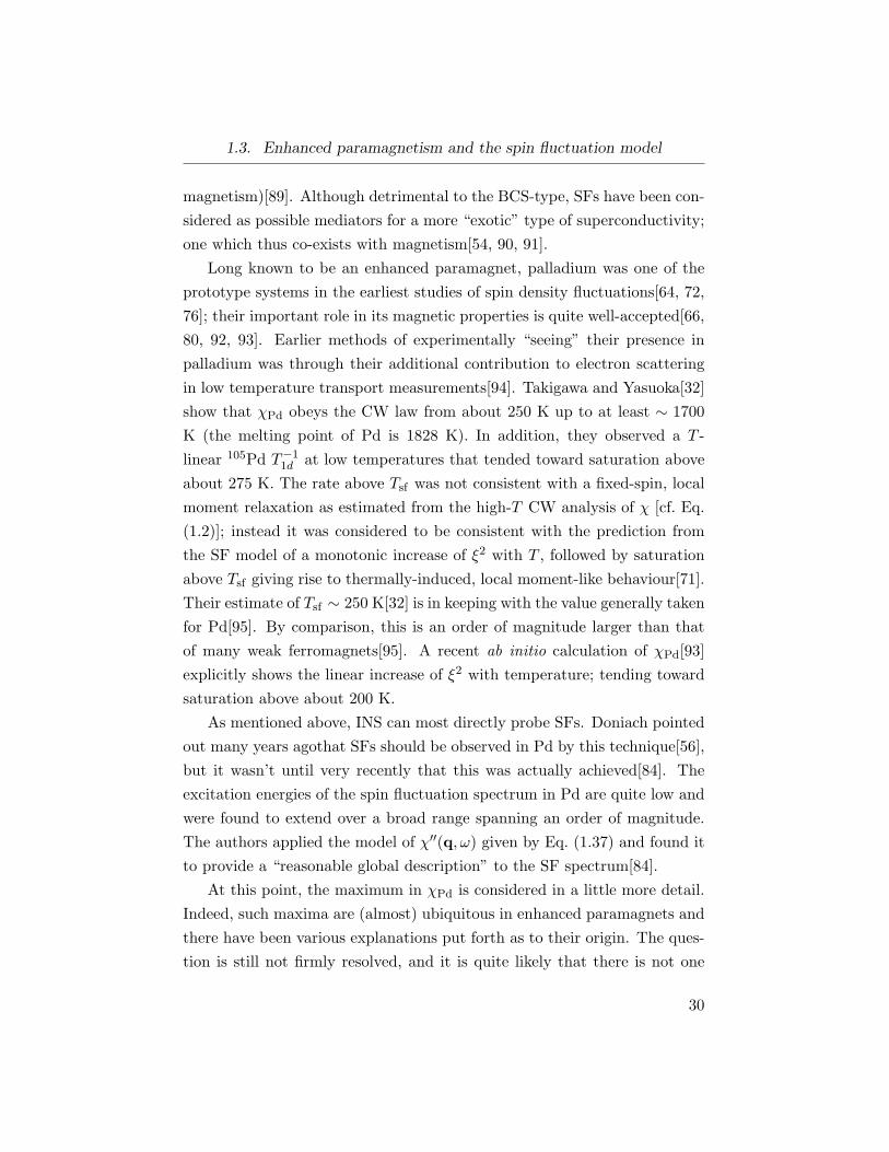
1.3. Enhanced paramagnetism and the spin fluctuation model
magnetism)[89]. Although detrimental to the BCS-type, SFs have been con-
sidered as possible mediators for a more “exotic” type of superconductivity;
one which thus co-exists with magnetism[54, 90, 91].
Long known to be an enhanced paramagnet, palladium was one of the
prototype systems in the earliest studies of spin density fluctuations[64, 72,
76]; their important role in its magnetic properties is quite well-accepted[66,
80, 92, 93]. Earlier methods of experimentally “seeing” their presence in
palladium was through their additional contribution to electron scattering
in low temperature transport measurements[94]. Takigawa and Yasuoka[32]
show that χPd obeys the CW law from about 250 K up to at least ∼ 1700
K (the melting point of Pd is 1828 K). In addition, they observed a T -
linear 105Pd T−11d at low temperatures that tended toward saturation above
about 275 K. The rate above Tsf was not consistent with a fixed-spin, local
moment relaxation as estimated from the high-T CW analysis of χ [cf. Eq.
(1.2)]; instead it was considered to be consistent with the prediction from
the SF model of a monotonic increase of ξ2 with T , followed by saturation
above Tsf giving rise to thermally-induced, local moment-like behaviour[71].
Their estimate of Tsf ∼ 250 K[32] is in keeping with the value generally taken
for Pd[95]. By comparison, this is an order of magnitude larger than that
of many weak ferromagnets[95]. A recent ab initio calculation of χPd[93]
explicitly shows the linear increase of ξ2 with temperature; tending toward
saturation above about 200 K.
As mentioned above, INS can most directly probe SFs. Doniach pointed
out many years agothat SFs should be observed in Pd by this technique[56],
but it wasn’t until very recently that this was actually achieved[84]. The
excitation energies of the spin fluctuation spectrum in Pd are quite low and
were found to extend over a broad range spanning an order of magnitude.
The authors applied the model of χ′′(q, ω) given by Eq. (1.37) and found it
to provide a “reasonable global description” to the SF spectrum[84].
At this point, the maximum in χPd is considered in a little more detail.
Indeed, such maxima are (almost) ubiquitous in enhanced paramagnets and
there have been various explanations put forth as to their origin. The ques-
tion is still not firmly resolved, and it is quite likely that there is not one
30
1.3. Enhanced paramagnetism and the spin fluctuation model
universal origin.
One line of thought attributes the maxima to T -dependent corrections to
the susceptibility due to scattering of electrons on the Fermi surface in the
presence of strong electron interactions[96, 97, 98, 99, 100, 101]. However,
throughout the years, there were often disagreements as to the exact form
and degree of importance of these corrections.
Within the SF model, a maximum in the susceptibility can arise if the
mode coupling parameter b is negative[71, 78]. Additionally, Yamada has
highlighted the role of negative mode-mode coupling in metamagnetism[89],
and in potential magnetovolume anomalies[102]. In such a case, Eq. (1.32)
must be carried out to include the M6 term[54]. This was recently illus-
trated by the susceptibilities of Ni3Al and Ni3Ga. The former is a weak
ferromagnet, while the latter does not order and is instead a strongly en-
hanced paramagnet. Smith found that the magnetization and susceptibility
of Ni3Al can be described using an expansion involving just the two Landau
parameters a and positive b (g ≡ 0); while the susceptibility of Ni3Ga was
best decribed with b negative, thus requiring all three parameters[79]. The
extended form of the expansion is a means of incorportating any low tem-
perature corrections; viewed as altering the effective interaction between the
fluctuation modes[103].
Within the SF model, the expansion coefficients can be derived micro-
scopically from the form of the band structure[71, 78]. This opens the
possibility of calculating these parameters ab initio[67, 80, 104, 105]. The
band structure itself is material-specific, and so features in the electronic
dispersion may play a role. For instance, if there are peaks, or singularities,
in the DOS close to EF , these can result in divergent quantities making ap-
plication of the model problematic[67]. The non-interacting DOS controls
the q dependence of the generalized susceptibility, and so directly influences
the SF spectrum[104].
According to the Stoner theory, χ(T ) of an enhanced paramagnet follows
a T 2 variation with a coefficient that is determined by the difference between
the second and first derivatives of DF with respect to E[58, 59, 69]. A DOS
that gives rise to a positive second derivative can lead to χ(T ) initially in-
31
1.3. Enhanced paramagnetism and the spin fluctuation model
creasing with T , thus exhibiting a maximum[69]. This criterion is indeed
found from the DOS of Pd[58, 59, 69], while DF itself decreases by approx-
imately 6% between 0 K and room temperature (due to thermal vibrations
of the atoms, i.e., phonons)[61]. Within the SF model, the mode coupling
parameter b is also determined by this same difference in the derivatives of
DF [71, 78, 106], where a positive second derivative is generally indicative of
a negative b. Thus, within this model, the maximum in χPd may require the
use of the extended expansion, as mentioned above. However, EF of Pd lies
just above a peak in the DOS. A strongly peaked DOS near the band edge
(dictated by the lattice structure) has been identified as being an important
condition for stabilizing ferromagnetism in general[57, 107]. In particular,
EF appears in a region of the DOS that is rapidly varying and near to an
inflection point[80, 109]. In calculations, this results in extreme sensitivity
of results to the placement of EF [58, 59, 60, 108, 109]. The second derivative
of DF is correspondingly a difficult quantity to calculate precisely[59, 80].
At the maximum, χPd is ∼ 10% larger than at T ≃ 0. It is conceivable
that such a small increase requires only a weak temperature dependence,
as, e.g., that found for DF [61]. For instance, in TiBe2, EF lies just below a
sharp peak in the DOS and it was concluded that the enhanced χ(T ) (which
varies more strongly with T than that of Pd) could be adequately described
by a T -dependent EF accompanied by thermal “smearing” of the DOS[67].
The possibility has been suggested that χPd(T ) can be completely described
within the Stoner (single particle) model for enhanced paramagnets if a
very accurate band structure is employed[109]. One method of improving
the agreement of the Stoner susceptibility with experiment is to allow for the
effective, mean-field exchange parameter I0 to be temperature-dependent.
In the past, such an approach has indeed been considered for the suscep-
tibility of enhanced paramagnets like Ni3Ga[110] and Pd[108, 111]. Most
recently, Zellermann et al.[109] employed this approach and succeeded in
reproducing χPd(T ) up to 800 K with the maximum appearing about 20 K
lower than experiment. In this case, it is found that the interaction param-
eter needs only a thermal variation ∼ 1% up to room T [109, 111], indicative
of the general adequacy of the Stoner model[109]. A weakly T -dependent
32
1.3. Enhanced paramagnetism and the spin fluctuation model
I0 may be viewed as an alternative way of dealing with small uncertainties
in the DOS and thus DF and its derivatives. In Ref. [109], the small varia-
tion of this quantity was interpreted as due to a renormalizing effect of the
collective thermal excitations; highlighting the close relation between the
single particle and collective effects, as the latter is strongly dependent on
the former.
In light of this, it is interesting to mention the renormalizing effects that
are attributed to the zero-point (zp) fluctuations in the spin fluctuation
models. In the earlier treatments[71, 78], they were assumed to produce a
T -independent renormalization of the interaction constant, I0 → I0; which
may be equivalently viewed as a renormalization of the DOS[78]. Subse-
quently, recent elaborations on the SF model have considered the role of the
zp fluctuations in more detail and have emphasized their influence on the
mode coupling parameter in particular[87, 112, 113, 115, 116, 117]. Miyai
and Ohkawa have argued that the CW susceptibility observed in itinerant
ferromagnets (especially those with on-site interactions strong enough that
the moments can be considered as “almost localized”) stems not only from
thermal spin fluctuations, but also from a temperature-dependent mean-
field interaction which occurs when there is a sharp peak in the DOS in the
vicinity of EF [118].
To close, the use of NMR to probe the spin fluctuation spectrum of a
metal is briefly summarized. In Sec. 1.2.2 above, T−11 was shown to de-
pend on the transverse fluctuations of the imaginary part of the dynamical
susceptibility [cf. Eq. (1.20)][39],
1
T1T=γ2
nkB
µ2Bh
∑
q
|Ahf(q)|2χ′′(q, ωL)
ωL. (1.40)
For definiteness Ahf(q) is taken to be independent of q. As the NMR fre-
quency is small, one can take the limit ωL → 0. Similarly, for the case of
q, one considers small values around the critical wavevector, as required
by the SF theories (q ∼ 0 for a ferromagnetic instability). Using the form
described by Eq. (1.38) leads to χ′′(q, ωL)/ωL ∝ χ(T )/Γ0; where χ(T ) is
33
1.3. Enhanced paramagnetism and the spin fluctuation model
the static uniform susceptibility [i.e., χ(0, 0)], and Γ0 represents the energy
scale of the SF spectrum.
As (T1T )−1 is typically dominated by the d electron (SF) contribution,
if the corresponding K − χ plot is found to be linear (at least over some T
range), then Kd(T ) ∝ χd(T ) and
(T1T )−1d ≃ κKd(T ) + y; (1.41)
where y is a constant off-set that accounts for the contributions from all
other less important relaxation processes. Ignoring the constants gives κ ∝(γ2
nAdhf)/Γ0 (recalling the Ad
hf can be determined from the slope of the K−χplot). This implies that a plot of 1/(T1T )d vs. Kd with T as the implicit
variable directly yields a slope that is inversely proportional to the energy
width of the SF spectrum. This linearity is a consequence of the dynamic
properties of metals close to, or possessing, a magnetically-ordered state (an
analogous scaling exists for antiferromagnets)[71, 119]. This behaviour is
clearly distinct from the Korringa relation [Eq. (1.26)], which is applicable
to simple metals that are far from a magnetic instability. The dynamical
scaling predicts a diverging zero-field T−11 as the critical T is approached,
reflecting the divergence in χ(T ) as the ordered state is approached[119].
The earliest report of 1/(T1T )d scaling with χd was from Ti NMR of
TiBe2[120], and has later been observed in a variety of metallic systems with
ferromagnetic[121, 122, 123, 124, 125, 126] and antiferromagnetic[85, 127]
SFs; the former including Pd[32]. The quantity Γ0 is equivalent to the
product cγm, and is expressed as a temperature denoted T0[71, 113]. The use
of NMR in this regard has encountered a very well-known issue associated
with the implementation of the SF theory itself; namely, the need to define
a cut-off wavevector qc. This quantity enters directly in converting Γ0 to
T0, or vice-versa. For instance, Corti et al. obtained a value of T0 from
Si NMR of MnSi that was a factor of four smaller than the value obtained
from INS[123]. The authors could obtain agreement if the value of qc used in
converting Γ0 was made four times larger than prescribed by the standard
SF model[123]. A similar conclusion about the need for a larger qc was
34
1.3. Enhanced paramagnetism and the spin fluctuation model
also recently reported from NMR measurements in a different system[125].
Since the SF models are based on small q expansions, the need to use a
large qc signifies a problem with the SF model in its original form. This is a
notable difficulty in applying the SF models as there is no exact definition of
qc[80, 86, 105], and the results are sensitive to the q range employed[71, 109].
1.3.1 Further notes on the susceptibility of Pd
It is noted that χPd does not show any dependence on applied field[128, 129,
130, 131], and that this is valid for fields as high as 40 T[95]. A tiny non-
linearity, i.e., increase, at high fields and low temperatures was reported
with a correction factor ∼ 10−14/G2[128]. This amounts to less than 1%
correction, and can safely be neglected[129, 130]. This is consistent with the
absence of a metamagnetic transition for Pd, in accord with calculations[92,
132, 133]. In Ref. [132] the critical field for this transition was predicted to
be ∼ 300 T.
The electronic structure, and therefore the magnetism of Pd is very sen-
sitive to the underlying lattice structure[134]. Since EF lies in a strongly
varying part of the DOS, even tiny changes in the lattice parameter can
have a large effect on DF [62]. One notable consequence of this is the
prediction that pure Pd will be ferromagnetic for a lattice expansion ∼5%[135, 136, 137, 138]. An expanded lattice results in a narrowing of the d
band and thus increased DF that, together with the high value of I0, will
satisfy the Stoner criterion for ferromagnetism. One experimental result at-
tributed to this effect was reported for thin Pd layers expitaxially strained
in the form of Au/Pd/Au sandwiches. Although the strained Pd did not
exhibit ferromagnetism, the low temperature susceptibility was significantly
enhanced: S ∼ 102 − 104[139]. It was concluded that the anisotropic nature
of the strain due to the two-dimensional nature of the samples plays an im-
portant role in this enhancement[140, 141, 142, 143]. In this regard, it has
been suggested that a strained lattice will also significantly reduce the criti-
cal field necessary for a metamagnetic transition[132]. Indeed, according to
Hjelm[133], lattice expansions of 2–5% cause the magnetization to increase
35
1.3. Enhanced paramagnetism and the spin fluctuation model
strongly as the applied field is increased from 0 to 50 T; for an expansion
of 5%, he predicts the critical field to be only 10 T. The potential influence
of lattice deformation on the susceptibility is important to keep in mind
when studying thin films of Pd, e.g., the β-NMR measurements presented
in Chapter 5.
Briefly, it is well-documented that the susceptibility of Pd is also sensi-
tive to the presence of impurities; in particular, all non-magnetic impurities
are known to cause χ(T ) to decrease. Overall, as the impurity concentra-
tion is increased, the magnitude of χ is reduced and the maximum becomes
less pronounced; eventually for sufficient impurity concentration, the maxi-
mum is completely eliminated and the susceptibility becomes temperature-
independent[11, 144, 145, 146, 147, 148, 149]. In general, the susceptibility
is reduced by a few per cent for every at.% of impurity. For example, in the
case of dilute Ag impurities, the initial reduction in the susceptibility is by
about 3% per at.% Ag, and the maximum in χ is essentially eliminated for
∼ 5 at.%[11, 148]. This reduction in the susceptibility applies to impurities
in the form of substitutional alloys, as well as interstitial impurities. The
latter is best illustrated by the susceptibilities of the hydrides[15, 150], as
Pd readily absorbs H (or deuterium) into the octahedral interstices. The
susceptibility is reduced by approximately 1.5% for each % of H(D) ab-
sorbed, essentially independent of temperature[150]. As the concentration
is increased above 60%, the maximum in χ is eliminated, resulting in a
T -independent susceptibility that eventually becomes diamagnetic[15]. A
similar reduction in χ has also been observed when B is introduced into
the octahedral sites[151]. A notable exception is dilute Rh impurities. In
the concentration range between 1 and 10 at.%, these substitutional alloys
show enhanced susceptibilities compared to that of the pure host, with a χ
that increases continually upon cooling below room temperature[13, 148].
Alloys with Rh concentrations between 3 and 8 at.% exhibit a susceptibility
at 4 K that is almost twice as large as that of Pd[148]. However, as the Rh
concentration is increased above 10 at.%, the susceptibilities of the alloys
again become reduced in comparison to Pd[13].
In contrast, since the susceptibility of Pd is so strongly enhanced, it has
36
1.4. An alternative: implanted probes
long been known that magnetic impurities like Fe and Ni readily generate a
ferromagnetic polarization of the conduction electrons, even in very dilute
concentrations[152]. A single magnetic impurity is sufficient to generate a
region of ferromagnetic polarization that encompasses a significant number
of surrounding host atoms. The localized moment together with the mo-
ment induced on the atoms within the polarized region (or “cloud”) give
rise to what is termed a “giant moment”[152, 153]. Fe impurities give rise
to the largest giant moments in Pd, with reported values of the effective
moment in the range of 7–15µB, depending on the concentration[153]. Neu-
tron diffraction measurements estimate the spatial extent of an Fe-induced
giant moment to be of the order of a nanometer in Pd[154]. A similar effect
occurs when magnetic impurities are introduced into Pt, but the size of the
giant moments are about half as large[153]. Thus, for sufficient concentra-
tions of magnetic impurities, the giant moments can percolate throughout
the volume of the host giving rise to a highly dilute alloy that can or-
der ferromagnetically. For Fe in Pd this occurs for concentrations ∼ 0.1
at.%[152, 155]. At this low concentration, TC is only around 5 K, but it
increases sub-linearly with increasing Fe, and appears to saturate at about
400 K in the more concentrated alloys (∼ 20 at.%)[155]. In the case of Ni,
a higher concentration ∼ 2 at.% is required to to drive Pd ferromagnetic;
however, in this case it is not isolated Ni atoms, but rather small Ni clusters
that are responsible for the induced ferromagnetism[156].
1.4 An alternative: implanted probes
While NMR is an attractive method to study the electronic structure of
materials (as it is in the study of molecules and liquids), it is not without
limitations. Specifically, signal-to-noise, i.e., low sensitivity imposes restric-
tions. In conventional NMR the signal is detected through changes in the
population of nuclear spin levels; the initial polarization produced by an ex-
ternal magnetic field and follows a thermal (Boltzmann) distribution. The
signal is frequently detected via the voltage induced in a pick-up coil (that
scales with ωL). As the degree of nuclear polarization is low, detection us-
37
1.4. An alternative: implanted probes
ing a macroscopic circuit requires there be a large number of spins; typically
∼ 1018. Besides the requirement of a sufficient amount of sample, in the
case of metals (i.e., conductors) there is a second consideration. The radio-
frequency (rf) magnetic field used to induce the spin population changes
can only penetrate into a metal a certain distance which is both material-
and frequency-dependent and is called the rf “skin depth”[157]. For metals,
this is typically of the order of microns. Consequently, NMR experiments
on metallic systems are most generally performed on samples in the form of
randomly-oriented powders.
In some cases, using fine-powdered samples can be desirable, since at very
small length scales the electronic structure is often distinct from that of the
macroscopic scale, and NMR can be used as an effective tool to study such
“finite-size effects” (see e.g., Ref. [5]). However, in real devices, materials
are often used in the form of thin films or multilayers. In this geometry both
a free surface and interfaces exist. Most generally, one can expect that the
electronic structure of a material will also be distinct from that of the bulk in
the vicinity of a surface or interface[158]. The change may be localized to a
single atomic layer, or it may exhibit a “healing length” in which it recovers
back to the bulk state over a distance of spanning several layers, perhaps in
an oscillatory fashion. While NMR does probe the electronic structure of
a material with atomic scale resolution, there is inherently a small number
of spins in the surface or interfacial regions, and this severely limits the
application of the technique to such samples. In the field of materials, NMR
is largely restricted to be a bulk probe of matter. This is troublesome
since there is an ever growing interest in materials of reduced dimensions
(i.e., size) for applications in electronics and catalysis, etc. Analogous to
powders, as a film becomes thinner, the surface or interface becomes an
increasing fraction of the total volume and in many cases the electronic
modification is intimately connected with this increase. There have been
some successful applications of NMR to the study of the interface between
two different metals[159], but such studies are certainly quite rare. One
method of extending the technique to the study of surfaces is to perform
NMR measurements on adsorbates that have been pre-polarized[160].
38
1.4. An alternative: implanted probes
A powerful alternative to conventional NMR in this regard is the use of
radioactive probes[161]. The outstanding advantage to such techniques lies
in the method of detection. Broadly, in these spectroscopies the signal is
detected through high-energy radiation emitted by a radioactive nucleus as
it undergoes decay. This in turn improves the signal-to-noise by orders of
magnitude. Consequently, far fewer spins are required making nuclear probe
techniques well suited for the study of samples consisting of a small number
of atoms. The probe nuclei are either implanted into the sample, or in some
cases, incorporated directly during synthesis. Frequently, this allows for the
possibility of studying condensed matter in a depth-resolved manner. The
implanted probes are sensitive to the local electronic structure of the host
through the various hyperfine interactions, in a fashion analogous to the hf
interactions of the host nuclei in conventional NMR (discussed above in Sec.
1.2).
In the present investigations one such nuclear technique, namely that of
beta-detected nuclear magnetic resonance β-NMR, has been applied to the
study of metallic paramagnetism. The technical and experimental details
are presented in Chapter 2 and Appendices A and B. Briefly, a low-energy
beam of 8Li+ (I = 2) is optically polarized in-flight and subsequently im-
planted into a sample. A variable, static, external magnetic field is applied
longitudinal to the nuclear spin and a magnetic resonance is detected by
the application of a small, transverse, rf magnetic field. The technique re-
lies on the anisotropic distribution of electrons emitted in beta-decay of the
probes. When the rf field is on resonance with the nuclear spin splitting,
the polarization is destroyed as the spin precesses in the rf field resulting
in a loss of the measured beta-electron count rate asymmetry. β-NMR can
be performed using ∼ 106 implanted spins; so, the probes are in the highly
dilute limit and interactions between them can be safely neglected.
The technique of β-NMR is very similar to the technique of muon spin
rotation/relaxation spectroscopy µSR[161, 162]. Typical µSR involves the
implantation of 2–4 MeV positive muons into a sample. In contrast, the
β-NMR spectrometer used for the present studies was specifically designed
to permit electrostatic deceleration of the low energy (∼ 30 keV) ion beam,
39
1.4. An alternative: implanted probes
and thus allow for variable implantation depths. This translates into the
ability to perform measurements on small length scales; for many materials
this ranges between ∼ 10 − 102 nm. Thus, systematic investigations as
a function of distance from a free surface, or from a buried interface are
readily possible. In this regard, low-energy β-NMR[163] is similar to low-
energy µSR[164]. As the static external field is not used to generate nuclear
spin polarization, the technique can in principle be performed for any value
of the applied field, including zero field (which in the case of I > 12 allows
for low-energy beta-detected nuclear quadrupole resonance β-NQR[165]).
One of the earliest, and still employed, applications of the β-NMR prin-
ciple is for the determination of the nuclear magnetic[166] or quadrupole
moments of an isotope[167]. The total hf field sensed by the implanted
probe is made up of contributions analogous to those of the host nuclei in
conventional NMR[161]: Fermi contact, as well as orbital, dipolar, and po-
tentially electric field gradients (EFGs). The Fermi contact interaction is
expected to be the source of the largest hf field at the nucleus and originates
from the coupling of the probe to the host electrons. For the case of a light
ion like 8Li+ in a transition metal, the dominant coupling is expected to
arise between the Li 2s orbital and the d band of the host[168]. In this way
a Knight shift and T−11 due to this coupling can be defined. The former
can be evaluated according to Eq. (1.16) using ν0 measured in a suitable
reference material, i.e., a diamagnetic insulator. Measurements of T−11 can
be made without the need for an rf magnetic field by monitoring the loss
of probe polarization with time following implantation. The dipolar inter-
action is discussed below, while the perturbation due to a EFG is discussed
in the following Chapter. For a light probe, the orbital interaction arises
from the motion of its electrons and is thus analogous to the chemical shift
in conventional NMR. Specifically, from 6,7Li NMR, these shifts are small;
typically in the range of -10 to +10 ppm[169].
The coupling between the probe and host can be quantified by a hf
40
1.4. An alternative: implanted probes
coupling constant defined as
Ahf =geµBNA
z
K
χP. (1.42)
In this form, Ahf is expressed in units of kG/µB. The variable z represents
the co-ordination number of the probe’s final stopping site in the host lattice,
so Ahf is a quantity that is expressed per atomic neighbour. This highlights
an important difference between conventional NMR and implanted probe
techniques like β-NMR, where following implantation, a light ion may come
to rest at distinct lattice sites in the host. For instance, it may occupy a reg-
ular lattice site arising from host vacancies created during the implantation
process, in which case it is considered a substitutional impurity. Alterna-
tively, it may remain in an interstitial site. This is an advantage of using
implanted nuclear probes as they offer access to the electronic structure of
the interstitial regions— which are more difficult to study by conventional
NMR. The strength of the hybridization is, in the simplest picture, a function
of z and the distance between the probe and the neighbouring host atoms,
in addition to the details of the electronic structure of the probe and host.
The NMR observables K, T−11 , linewidths, and (where applicable) EFGs,
will thus depend sensitively on the probe’s stopping site. Additionally, Ahf
is sensitive to factors like the degree of electronic screening in the immediate
vincinity of the probe by the electrons of the host, and to the extent of local
host lattice relaxation around the probe. Results from measurements of the
hf field at implanted probes provide stringent tests for electronic structure
calculations[170, 171, 172]. One can perform a Korringa analysis [i.e., Eq.
(1.26)] on the Knight shift and T−11 measured for an implanted probe and
compare the degree of electronic enhancement at the probe with that for the
matrix nuclei obtained by conventional NMR (when available)[173, 174]. For
the case of 8Li, S0 = 1.20 × 10⁻⁵ s K in Eq. (1.26).
One of the main challenges in interpreting results from a light implanted
probe is thus the unambiguous determination of the final stopping site(s).
Muons are interstitial probes and heavy ions are generally substitutional,
but lighter nuclei like 8Li and 12B can possibly occupy both interstitial and
41
1.4. An alternative: implanted probes
substitutional sites. In this respect, the dipolar interaction can be useful.
Specifically, the nuclear dipole-dipole interaction between the probe spin
and host spins may be the dominant mechanism giving rise to a broadening
of the resonance. The magnitude of the interaction depends on the lattice
site, as well as the crystallographic orientation. By using single crystal
samples the direction of H0 can be varied with respect to the crystal axes
and the resulting linewidths compared with those predicted from van Vleck’s
expression for dipolar line broadening due to unlike spins[20, 175],
σ2dip =
1
3γ2
Iγ2S h
2S(S + 1)∑
i
(3 cos2 θ − 1)2
r6i, (1.43)
where r is the distance vector from the probe spin I and the host spin S,
θ the angle between r and H0, and the sum runs over a given number of
neighbouring lattice shells. However, if the host spins possess a quadrupole
moment, the above equation does not necessarily hold because the presence
of a charged probe generates an EFG on the surrounding host nuclei that in-
fluences the orientational dependence of the dipolar widths[176]. Eq. (1.43)
is applicable only for sufficiently strong H0, i.e., such that the magnetic Zee-
man energy is larger than the electric quadrupole energy for the neighbour-
ing host spins[176, 177]. The dipole-dipole interaction provides the basis for
an alternative method by which the stopping site can indeed be unambigu-
ously determined. Briefly, when the host spins are quadrupolar, the EFG
induced by the probe permits the possibility that, for particular finite values
of H0, the energy of the |∆mI | = 1 transition for the probe and host spins
are equal. When this condition is satisfied, the probe and host spins can
undergo mutual spin flips resulting in the transfer of polarization from the
probe to the host spin system, a process termed cross-relaxation[178, 179].
The resonance-like loss of probe polarization at specific values of H0 pro-
vides a “fingerprint” of the stopping site for a given crystal orientation with
respect to the applied field.
In the application of implanted probe NMR to the study of fcc metals
resonances are almost always observed without satellites, being indicative
42
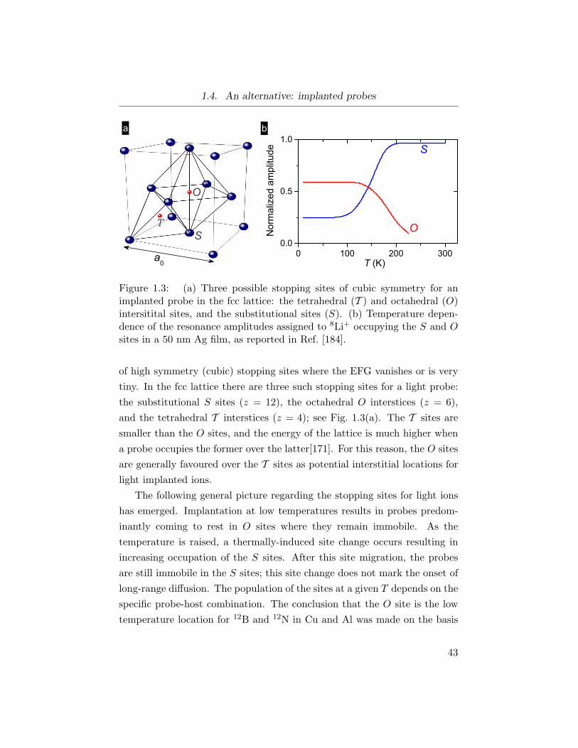
1.4. An alternative: implanted probes
Figure 1.3: (a) Three possible stopping sites of cubic symmetry for animplanted probe in the fcc lattice: the tetrahedral (T ) and octahedral (O)intersitital sites, and the substitutional sites (S). (b) Temperature depen-dence of the resonance amplitudes assigned to 8Li+ occupying the S and Osites in a 50 nm Ag film, as reported in Ref. [184].
of high symmetry (cubic) stopping sites where the EFG vanishes or is very
tiny. In the fcc lattice there are three such stopping sites for a light probe:
the substitutional S sites (z = 12), the octahedral O interstices (z = 6),
and the tetrahedral T interstices (z = 4); see Fig. 1.3(a). The T sites are
smaller than the O sites, and the energy of the lattice is much higher when
a probe occupies the former over the latter[171]. For this reason, the O sites
are generally favoured over the T sites as potential interstitial locations for
light implanted ions.
The following general picture regarding the stopping sites for light ions
has emerged. Implantation at low temperatures results in probes predom-
inantly coming to rest in O sites where they remain immobile. As the
temperature is raised, a thermally-induced site change occurs resulting in
increasing occupation of the S sites. After this site migration, the probes
are still immobile in the S sites; this site change does not mark the onset of
long-range diffusion. The population of the sites at a given T depends on the
specific probe-host combination. The conclusion that the O site is the low
temperature location for 12B and 12N in Cu and Al was made on the basis
43
1.4. An alternative: implanted probes
of dipolar linewidths[180, 181]. By means of the cross-relaxation method,
a definitive assignment of 12B to the O site in Cu and Al was made[182],
as well as its thermal migration to the S in Cu[179]. On account of the
r−6 dependence of σdip it was concluded that 12B and 12N in the O site
of Cu or Al produces a local lattice expansion ∼ 10%[181, 183]. Similarly,
when a smaller ion occupies the S site, a local lattice contraction may be
expected[179], as was indeed reported for 12B in ZnSe[177]. The local lattice
relaxation about an implanted ion is thus a significant factor contributing
to the hf interactions sensed by the probe[168, 170, 171, 181, 183].
Results from 8Li β-NMR of fcc metals Ag[184], Cu[185], Al[186], and
Ni[172] have been interpreted in terms of these site occupations as a func-
tion of temperature. At low T , resonances at two dinstinct frequencies are
observed. The higher frequency resonance is assigned to ions in the O sites,
since as T is increased, this resonance gradually decreases in amplitude con-
comitant with an increase in the amplitude of the lower frequency line, thus
assigned to S ions. In many hosts, for T on the order of room temperature,
only resonances from ions in the S site are observed. This is illustrated in
Fig. 1.3(b) by the normalized amplitudes of the resonances recorded in a Ag
film as a function of T [184]. Correspondingly, this site change behaviour is
manifest in the spin-lattice relaxation rates: T−11 is observed to be linear
with T— consistent with the Korringa mechansim described in Sec. 1.2.2
above— with a gradual decrease in slope over the T interval where the ions
undergo the O → S site change[185, 186, 187]. The occupation of S sites
arises from ions that have encountered a host vacancy created during the im-
plantation process, since this resonance can be observed even at low T . It is
pointed out that the site change may not be due to migration of the Li itself;
instead, S sites may be generated through combination with a thermally-
migrating host vacancy created during the ion implantion. Regardless, the
supply of host vacancies available to a probe most generally must have been
created during the implantation process as the energy required for the for-
mation of an intrinsic self-vacancy in metals is quite high[188].
The goal of the research presented herein is to apply the technique of low-
energy β-NMR to study of the magnetism of pure transition metals, thereby
44
1.4. An alternative: implanted probes
demonstrating the utility of this technique in extending the application of
NMR for investigations of this important property. Specifically, to illustrate
the applicability of β-NMR to the study of magnetism in systems where
conventional NMR is difficult or most generally not possible, like samples in
the form of films, or for metals like Pd. To this end, results of 8Li β-NMR
of non-magnetic Au are also presented and serve as a contrast to those of
the enhanced paramagnetism of Pd. The samples studied are chosen to be
representative of the bulk properties of these metals in order to establish a
firm understanding of the behaviour of the 8Li+ probe in the bulk metallic
state. The term bulk is employed here to mean samples sufficiently thick
that no finite-size effects are expected (in general, greater than ∼ 10 nm).
This serves as an important prerequisite to any future β-NMR investigations
of samples of reduced geometry.
In the case of Au, the study completes the 8Li β-NMR of the group 11
(or noble metals) and the results can be compared with those obtained in
Ag[184] and Cu[185]. There exists no previous 8Li β-NMR study of Au as
a function of temperature. In Ref. [166] a resonance and T−11 measurement
were made at room T towards the determination of the 8Li magnetic dipole
moment; a separate room T measurement of T−11 was also later reported for
8Li in this host[189]. A β-NMR study of Au using 12B was performed for
temperatures in the range of 100 – 300 K[173].
The study of these simple, non-magnetic metals in their pure, bulk form
is important as they are often used as spacer layers in magnetic multilayer
heterostructures. For example, the magnetic coupling between two ferro-
magnetic layers separated by a non-magnetic metal layer can be tuned by
changing the thickness of the latter. Such heterostructures can thus be used
for spin-dependent transport applications. The depth resolution capabilities
of low-energy β-NMR make it quite well-suited for the study of the mag-
netic interactions in such multilayers. Indeed, the spatial dependence of the
induced magnetism in a Ag layer in contact with a ferromagnetic Fe layer
has already been successfully studied by low-energy β-NMR[190].
Owing to its chemical inertness, Au is frequently used as a capping layer
for thin film samples. A powerful application of low-energy β-NMR is the
45
1.4. An alternative: implanted probes
study of magnetism at surfaces by implanting the probes in a thin, non-
magnetic metal overlayer and monitoring the magnetic behaviour proximally[191].
This has recently been accomplished for the case of a Ag overlayer on a high-
temperature superconductor[192]. The more frequent use of Au protective
layers make it potentially more attractive for such studies. A detailed study
of the 8Li resonances in pure Au is thus clearly required for such an appli-
cation.
A very different situation is to be expected in the case of an enhanced
paramagnet like Pd. The electronic structure of this metal is highly sensitive
to its lattice structure, and recently ferromagnetism has been reported for
samples in the form of thin films[193] and small particles[194]. Conventional
NMR of Pd is most generally not feasible in these cases, and so low-energy
β-NMR is an ideal alternative. However, this same sensitivity of Pd requires
an initial clear understanding of the response of this metal to the implanted
ion itself.
Just as in the case of Au, there have previously been only two room
temperature β-NMR measurements of 8Li in Pd, i.e., Refs. [166, 189]. Based
on their determination of the 8Li magnetic moment, the authors of Ref. [166]
concluded that K is negative for this probe in Pd, and that K at 300 K is
≃ 6. The remaining implanted probe studies of Pd have been performed
with 12B and 12N[195, 196] or µ+[197, 198]. In Ref. [196], the 12B and 12N
measurements were performed for temperatures in the range of 100 – 600 K
and a linear K − χ scaling was observed for both probes; the shift of 12N
was found to be positive for all T , while that for 12B changed from negative
to positive at T ≈ 400 K. Additionally, for both probes the observed shifts
were notably enhanced over that predicted from the measured T−11 and the
Korringa relation. In the case of µ+, the reported shifts are negative[197,
198]. In Ref. [198] data were collected for T extending up to 900 K, and
an overall linear K − χ scaling was also observed, except for T below the
maximum, where the shifts do not appear to track the decrease in χ as
closely. The results of the positive muon K for T below room temperature
are also included for comparison in Fig. 1.2.
A close similarity between the magnitude of K in Pd and the magnitude
46
1.4. An alternative: implanted probes
of the hf field in Ni as a function of the impurity valence for Cu, Al, Sn,
and µ+ has been observed experimentally[170, 197]. This similarity illus-
trates that the hf fields in a strongly enhanced paramagnet are physically
similar[170]. Calculations predict the hf field for 8Li impurities at all three
cubic lattice sites in Ni to be negative[171]. Indeed, in the β-NMR of 8Li
in Ni, two resonances were observed both with negative K, being assigned
to ions in the O and S sites[172]. Briefly, the negative hf field at a non-
transition impurity in a ferromagnetic host can largely be rationalized in
terms of a core polarization-like process for the bonding electrons between
the probe and host via the s− d hybridization[170].
The above serves as a general summary of important aspects of the β-
NMR of metals. The following Chapter is devoted to further details of the
technique.
47
Chapter 2
The β-NMR Technique (at
TRIUMF)
2.1 Introduction
In the previous chapter, the advantages of using implanted radioactive ions
as probes of matter in over-coming the limitations of convention NMR to
study thin films, or surfaces and interfaces was discussed. As β-NMR is a
rather “exotic” technique, the present chapter is devoted to a description of
this spectroscopy with respect to the TRIUMF facility.
The most basic requirement of β-NMR is the ability to produce an iso-
topically pure beam of the desired radioactive ion. This need is met at the
TRIUMF’s ISAC (Isotope Separator and ACcelerator) facility. Following a
brief sketch of the production of the radioactive ion beam (RIB), the prin-
ciples of the optical polarization of the 8Li probe will be described, and
then the basics of β-NMR data collection and analysis will be detailed.
This chapter ends with a discussion of three topics important to β-NMR:
rf power-broadening of resonances, the macroscopic demagnetization correc-
tion to the shift of a resonance, and the effect of a quadrupolar interaction
on the resonance spectrum.
2.2 Production and polarization of 8Li
2.2.1 Isotope production
RIBs are produced at ISAC using the 500 MeV proton beam from the TRI-
UMF cyclotron (the actual accelerated species are H− ions; the electrons
48
2.2. Production and polarization of 8Li
are stripped by graphite foils before the protons enter the beam line). The
proton beam is used to drive a secondary RIB using the ISOL (isotope
separation on-line) technique. The high-energy protons bombard a target
(typically SiC or Ta) and induce various spallation reactions. The isotopes
produced diffuse out of the target, promoted by maintaining the target at
a high temperature (∼ 2500 ◦C). The nuclides are then ionized by contact
with a heated tungsten extraction tube (this works well for species with low
ionization energies, like the alkalis). The target is typically held at a voltage
of 28–30 keV. The nuclides thus escape the target with this energy, having
a spread of 1–2 eV. This small energy spread is important for subsequent
transport and optical polarization with high efficiencies. The production
of radioactive isotopes is accompanied by high radiation fields, and there-
fore, the entire target stations are located underground, shielded from the
experiment hall.
After extraction from the target and ionization, a beam of the desired
isotope is obtained using mass separators. These are essentially a series
of magnetic fields that causes a deflection of the ions’ path based on their
mass-to-charge ratio. This occurs in stages; in the first a coarse separation
is achieved, while in the second, a pair of magnets provides a very high
resolution of mass separation. The resolution of the ISAC mass separators
is more than enough for a light isotope like 8Li (there are no stable isobars
with this mass number for which 8Li is the longest-lived radioactive species).
Upon exiting the mass separators, the ion beam is then directed above
ground to the appropriate experiment station. Transport of the beam is
accomplished using electrostatic focussing and “steering” elements. The
entire beam line is maintained under high vacuum.
2.2.2 Polarization of the 8Li nuclear spin
β-NMR relies on the ability to regularly achieve a high degree of nuclear
polarization. In this regard, the process of polarizing the probes underpins
the technique. The radioactive ion beam for β-NMR is polarized by optical
pumping using circularly polarized light; a process suggested by A. Kastler
49
2.2. Production and polarization of 8Li
in the early 1950s, that is particularly suited to atoms like alkalis[199, 200].
At ISAC this nuclear polarization is accomplished using in-flight, collinear
optical pumping[201]. The overall process involves three main steps[201]:
neutralization of the 8Li+ ions; optical pumping of the neutral atoms using
a counter-propagating, circularly polarized, resonant laser beam; followed
by re-ionization of the atoms. The important points of the process are
described below, aided by the optical pumping scheme for the 8Li atom and
the layout of the ISAC polarizer, shown in Fig. 2.1 (a) and (b), respectively.
The 8Li+ ions are first neutralized resulting in a beam of 8Li0 (valence
electron configuration 2s1). This is achieved by passing the beam through
a cell of Na vapour, typically held at about 480◦C. 8Li+ has a large cross
section for charge exchange with Na[163], and under typical conditions the
beam is neutralized with ∼ 50% efficiency. The neutral beam then drifts
through the optical pumping region (1.7 m in length) in the presence of a
small, longitudinal magnetic holding field of 1 mT, maintaining the nuclear
polarization axis. Situated in the drift region is an electrostatic deflection
plate that removes any ions that exit the Na cell without becoming neutral-
ized.
Atomic excitation occurs along the drift region through the interaction
of the beam with the counter-propagating laser that is right- or left-handed
circularly polarized with respect to the magnetic holding field/beam mo-
mentum axis. Atomic excitation occurs by irradiating the Li D1 transition
between the 2S 12
ground state and the 2P 12
first excited state that occurs
at a wavelength of 671 nm. The optical pumping is carried out by a single-
frequency dye laser that is itself pumped by a Nd:YAG laser. The laser
laboratory is located under the experiment hall and the light is directed
by mirrors up to the beam line. A linear polarizer in combination with
a remotely-controlled quater-wave plate allow for switching of the helicity
(positive or negative) of the excitation light (i.e., right- or left-handed cir-
cular polarization) before it enters the beam line.
As shown in Fig. 2.1(a), both the 2S 12
ground state and 2P 12
first excited
state are split by interaction of the single valence electronic spin with the8Li nuclear spin (I = 2) giving rise to two hyperfine levels that correspond
50
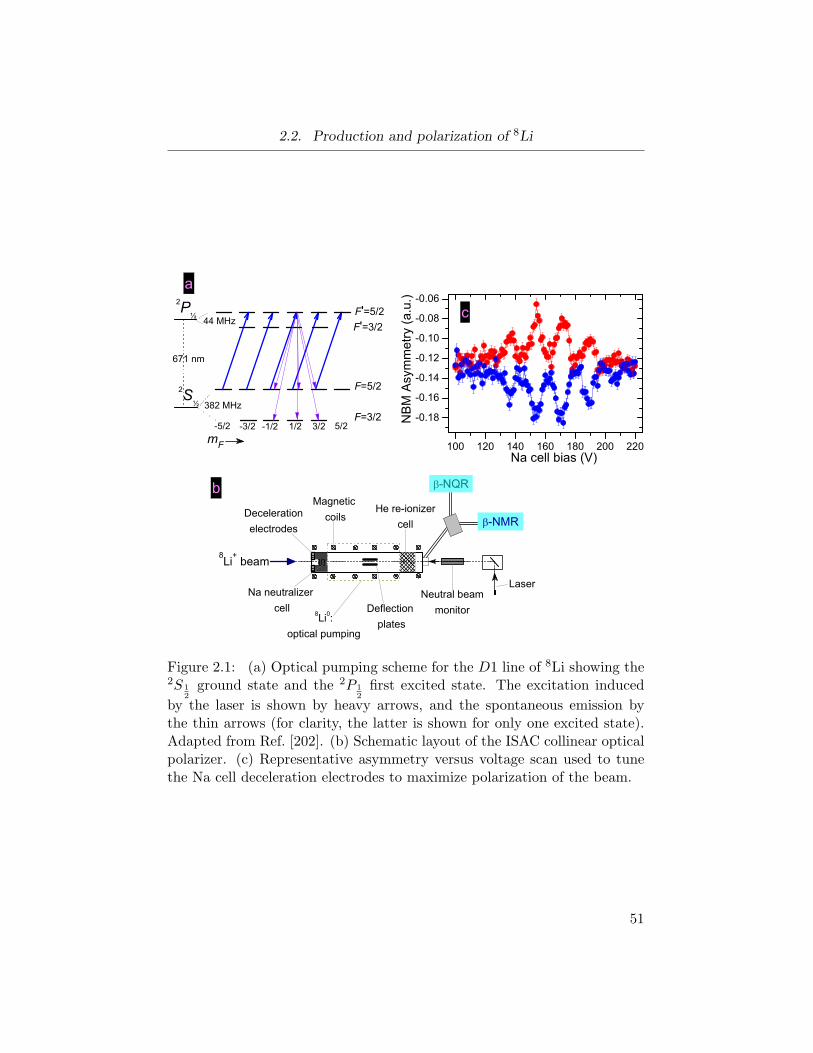
2.2. Production and polarization of 8Li
Figure 2.1: (a) Optical pumping scheme for the D1 line of 8Li showing the2S 1
2ground state and the 2P 1
2first excited state. The excitation induced
by the laser is shown by heavy arrows, and the spontaneous emission bythe thin arrows (for clarity, the latter is shown for only one excited state).Adapted from Ref. [202]. (b) Schematic layout of the ISAC collinear opticalpolarizer. (c) Representative asymmetry versus voltage scan used to tunethe Na cell deceleration electrodes to maximize polarization of the beam.
51
2.2. Production and polarization of 8Li
to the spin state of the valence electron: F = (I + J); F (′) = 32 ,
52 . The
splitting is 382 MHz in the ground state and 44 MHz for the excited state.
In the presence of the ∼ 10 G external holding field, the hyperfine levels
are further split into four (F = 32) and six (F = 5
2) sublevels, according
to their magnetic quantum numbers mF . Since the field is small, these
sublevels are almost degenerate with respect to the hyperfine splitting[202].
Absorption of a photon of, e.g., positive helicity, excites the Li atom from
the ground state according to the selection rule ∆mF = +1, and the atoms
decay by spontaneous emission according to the selection rule ∆mF = 0,±1.
After many cycles of excitation and emission, the angular momentum carried
by the absorbed photons is transferred to the atoms[199, 200, 202]. The
resonant atoms are thus “pumped” towards increasing atomic (and nuclear)
polarization, i.e., increasing mF . The lifetime for spontaneous fluorescence
of the excited state is about 50 ns, which is short compared to the transit
time through the optical pumping region (∼ µs). Consequently, when the
atoms reach the end of this region, they have undergone multiple pumping
cycles and are highly polarized; the majority occupy the (F = 52 ,mF = +5
2)
state corresponding to the nuclear spin state mI = +2[163, 202], which
is antiparallel to the beam momentum. Thus, if the excitation light is of
negative helicity (∆mF = −1), the nuclear spin state is mI = −2, parallel
to the beam momentum as a result of pumping to the (F = 52 ,mF = −5
2)
state [i.e., for this case the heavy arrows in Fig. 2.1(a) point to the left].
The last step is to re-ionize the beam by passing it through a cell of
He gas, ionizing the 8Li0 with an efficiency of ∼ 50%. This allows for elec-
trostatic steering/focussing of the now spin-polarized 8Li+ beam. The nu-
clear polarization is preserved during the stripping process. Two 45-degree
electrostatic bends that preserve the longitudinal nuclear polarization are
located immeditately after the He cell. Any Li not re-ionized are unaffected
by the first of these bends, and instead continue in a straight path into
the neutral beam monitor (NBM). This apparatus is comprised of a metal
foil in a 20 mT longitudinal holding field. There is an aperture in the foil
through which the laser beam passes into the beam line. Two detectors in
a backward-forward geometry (same as that of the β-NMR spectrometer
52
2.2. Production and polarization of 8Li
described in following Section), are used to monitor the polarization and
relative intensity of the neutral beam, and as such, the NBM provides an
important diagnostic of the 8Li+ beam used in the experiments.
A couple of important aspects of the optical pumping process also deserve
mention. In order to maximize the nuclear polarization, pumping of both
hyperfine levels of the 2S 12
ground state simultaneously is required, and this
is achieved by modulating the frequency of the laser[201, 202]. The laser is
passed through an electro-optic modulator (EOM) operating at the hyperfine
splitting to generate first-order sidebands at that frequency and broaden
the effective bandwidth of the pumping light. Additionally, the resonant
absorption frequencies of the Li atoms become Doppler-broadened since they
are emitted from the target with a distribution of thermal energies. For an
ion beam of energy Ei, with a width of ∆Ei, the Doppler width of the
absorption frequency ∆ν∗ can be described by[163] ∆ν∗/ν∗ ∝ ∆Ei/√Ei.
Recall from above, for the 8Li beam Ei=28–30 keV with ∆Ei ≈ 2 eV, and so
accelerating the beam reduces the relative Doppler broadening thus reducing
the required laser power[163]. However, Doppler broadening also occurs due
to the multiple collisions with the Na atoms of the neutralizer which can
be ∼ 100 MHz[201]. This broadening is significant enough to prevent the
resolution of the first excited state hyperfine splitting[202]. To overcome
this, after the laser passes through the first EOM, it then passes through
two more EOMs operating in series at 28 and 19 MHz which generate higher-
order sidebands. The result is multiple sidebands with a spacing ∼ 10 MHz,
and this allows for the Doppler-broadened absorption spectrum to be covered
by the excitation light[201].
In order to maintain a high degree of nuclear polarization the laser fre-
quency must remain stable over the course of spectra collection. This is ac-
complished by the use of an interferometry (etalon) feed-back system based
on the frequency difference between the dye laser and a frequency-stabilized
HeNe laser. This prevents the excitation frequency from drifting more than
a few MHz per day[201]. Once the laser is tuned and stabilized, the atomic
beam energy is fine-tuned in order to match the Doppler shifted absorption
resonance to the laser frequency. This is done by scanning the beam en-
53
2.3. The β-NMR spectrometer
ergy through the use of deceleration electrodes located at the entrance of
the Na cell. Fig. 2.1(c) shows an example of such a scan, where the asym-
metry from the two laser helicities (proportional to the optically-generated
nuclear polarization) measured at the NBM is plotted against the deceler-
ation bias voltage applied to the electrodes. The multiple peaks originate
from scanning of the ground state hyperfine levels across the sidebands of
the excitation laser; the largest peaks corresponding to the pumping of both
levels[201, 202], which determines the bias value for maximal polarization.
Should the laser need to be re-tuned, the Na cell bias scan is re-performed to
determine the new optimal voltage. The example in Fig. 2.1(c) is quite typi-
cal; the applied deceleration voltage is generally ∼ 0.1 kV, a small correction
to the nominal Li beam energy.
The continuous-wave laser power used is typically ∼ 100 mW. Nuclear
polarization ∼ 70% is routinely obtained; while values as high as 80% are
attainable, but at the expense of overall ion beam intensity. This value of
the nuclear polarization produced is expressed in terms of the normalized
nuclear magnetic sublevel population[202]
P =1
I
∑
m
mpm, (2.1)
where m is the nuclear magnetic quantum number and pm is the population
of the corresponding sublevel. The vector polarization being defined with
respect to the longitudinal holding field taken along the z direction. As
described in the next Section, the same longitudinal geometry applies to
the spectrometer; the optically-generated nuclear polarization along this
direction is denoted by P0.
2.3 The β-NMR spectrometer
The spectrometer is of longitudinal design, i.e., the beam axis (and nu-
clear polarization) are collinear with the external magnetic field H0; see Fig.
2.2(a). The spectrometer operates under ultra-high vacuum (UHV,<∼ 10−9
Torr). This is an important requirement, otherwise the Li ions (and emitted
54
2.3. The β-NMR spectrometer
β-electrons) would stop in contaminant, residual gases (easily condensed at
cryogenic temperatures). This spectrometer is also known as the “high-field”
spectrometer as H0 can be as large as 9 T. The field is produced by a high-
homogeneity superconducting solenoid. Broadly, in addition to the solenoid,
the other important components of the spectrometer are the He cold-finger
cyrostat (3–310 K), a coil to apply the radio-frequency H1 (associated fre-
quency generator and amplifier), and two fast plastic scintillator detectors.
The layout of the spectrometer is sketched in Fig. 2.2(a); a schematic may
be found in Ref. [163]. Side-view images of the spectrometer, and an axial
view image of the cryostat (outside the UHV chamber) are also displayed in
Fig. 2.2.
The two detectors are located upstream (backward) B, and downstream
(forward) F of the sample. As the probes’ momentum is longitudinal to
H0, the ions must enter the spectrometer and reach the sample by passing
through a 1.5 cm aperture in the B detector. Both detectors are made from
(Bicron BC412) plastic. Note Fig. 2.2(a) is not to scale; in reality the B
detector is outside the solenoid, further away from the sample than the F
detector. Thus, the solid angles subtended by the detectors are different,
resulting in different efficiencies. However, the presence of a high magnetic
field has a focussing effect on both the incoming 8Li+ and the emitted betas,
resulting in a circular motion of the particles perpendicular to the field; i.e.,
a helical trajectory[157] that confines them along the axis of the solenoid.
This effectively increases the solid angle of the B detector such that the
efficiencies of the two detectors are similar when the applied field is above
about 1 T.
These are telescope scintillator detectors. The photons generated when
β-electrons strike the plastic are transmitted via lucite light-guides to pho-
tomultiplier tubes (PMTs). These in turn convert the optical signal into an
electrical pulse to be digitized for computer storage. The detectors and their
light-guides are housed in stainless steel, with thin stainless steel windows
(0.05 mm thick) through which the MeV β-electrons can easily pass. This
casing isolates the detectors from the UHV.
The cryostat is attached to a motorized bellows that allows it to be
55
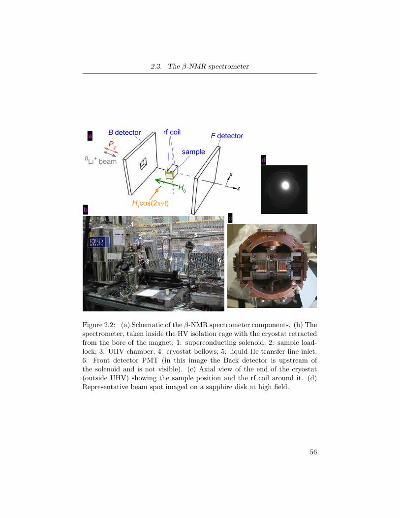
2.3. The β-NMR spectrometer
Figure 2.2: (a) Schematic of the β-NMR spectrometer components. (b) Thespectrometer, taken inside the HV isolation cage with the cryostat retractedfrom the bore of the magnet; 1: superconducting solenoid; 2: sample load-lock; 3: UHV chamber; 4: cryostat bellows; 5: liquid He transfer line inlet;6: Front detector PMT (in this image the Back detector is upstream ofthe solenoid and is not visible). (c) Axial view of the end of the cryostat(outside UHV) showing the sample position and the rf coil around it. (d)Representative beam spot imaged on a sapphire disk at high field.
56
2.3. The β-NMR spectrometer
retracted from, or inserted into, the bore of the superconducting solenoid.
This allows access to the sample through a load-lock such that samples may
be changed without the need to vent the entire UHV chamber. The sample
holder port in the cryostat is keyed such that only the front of the sample
faces the ion beam.
As mentioned in the previous Chapter, an important capability of the
β-NMR spectrometer is the electrostatic deceleration of the 8Li+ beam,
thereby allowing for variable implantation depth and thus depth-resolved
measurements. Deceleration is accomplished by placing the entire spectrom-
eter and associated electronics on a high-voltage platform that is electrically
isolated from ground. The bias voltage is thus an adjustable electrostatic
barrier (up to 30 kV) that the Li ions must overcome, reducing their momen-
tum before they reach the sample. For safety purposes, the platform and
components on it, are housed in an interlocked “cage,” portions of which
are visible in Fig. 2.2(b).
2.3.1 Some comments on beam spot tuning
As discussed above, after exiting the He re-ionization cell of the polarizer
the beam is transported and focussed onto the sample by means of the
electrostatic beamline optics. Directly upstream of the spectrometer is a
series of three variable-width collimators through which the beam passes
before travelling through the B detector hole and the final Einzel lens. This
Einzel lens and the strong fields of the solenoid are used to focus the beam
onto the sample. Ideally, a tightly-focussed and centred beam spot is desired.
Typically, the beam spot is circular and ranges between 2–3 mm in diameter.
For a given ion energy, the size and location of the beam spot are quite
sensitive to the applied Einzel lens voltage (≤ 20 kV) and the external field.
When the external field is high (> 0.3 T), the Einzel voltage is restricted
due to electric discharge problems; since experiments with the β-NMR spec-
trometer frequently utilize large H0, it is the solenoid that provides most of
the final focussing.
Time is invested at the outset of all experiments to ensure the optics
57
2.4. Data collection and analysis
of the entire beam line are tuned to provide the best beam spot under a
variety of conditions, e.g., various fields and/or platform biases. To verify
the position and size of the beam spot relative to the sample, images of the
spot striking a crystalline sapphire disk (which is found to scintillate) are
taken using a CCD (charge-coupled device) camera. The sapphire disk is
mounted at the end of the cryostat and can be rotated in front of the sample
when the cryostat is retracted [not shown in Fig. 2.2(c)]. The camera is
mounted upstream of the sample, normal to the beam axis. Images of the
beam spot are recorded by reflecting the scintillation light toward the camera
using a mirror also mounted inside the beam line. An example of such an
image is shown in Fig. 2.2(d). By removing the scintillator disk, and using
illumination provided by LED lights located inside the beam line, similar
images of the sample itself may be collected. The camera software allows
for quantitative comparisons of the sample and beam spot centres.
In general, when the spectrometer bias is raised to lower the incident en-
ergy, the spot tends to become more diffuse. The combination of magnetic
field from the solenoid and the beam energy determine the beam envelope
function which oscillates along the trajectory toward the sample. A beam
transport simulation program has been developed at ISAC that can success-
fully predict combinations of “magic fields” and final energies for which the
beam envelope is a minimum (a node) at the the plane of the sample. For
this reason, spectra are collected at particular combinations of H0 and ELi.
2.4 Data collection and analysis
In this Section, a general description of the procedures for recording reso-
nance spectra (a function of frequency), and spin-lattice relaxation spectra
(a function of time) are described. However, for both types of spectra, the
important observable is the asymmetry A in the detector counts. As men-
tioned previously, this asymmetry is a result of the nonconservation of parity
in β-decay, and is thus pivotal to β-NMR.
In Fig. 2.2(a), the large, static external field H0 defines the polarization
axis z to which the 8Li+ nuclear polarization is collinear. As described above,
58
2.4. Data collection and analysis
depending on the helicity of the laser light, the ions are either implanted with
their polarization parallel or antiparallel to their momentum. For 8Li the
β-electrons are emitted preferentially opposite to the nuclear polarization.
Referring to Eq. A.9 [and Fig. A.2(b)], for the longitudinal geometry of the
β-NMR spectrometer (detection angles 0◦ and 180◦), the β-electron count
distribution in the two dectors follows[202, 203]
NF (B) = αF (B)[1 ±AP ], (2.2)
whereNF (B) is the number of counts at a given detector, A for 8Li is −13 [201],
and the constant αF (B) is an experimental factor that takes into account the
detector geometry and efficiencies.
The measured asymmetry in the β-electron counts is thus directly pro-
portional to the nuclear polarization. The resulting normalized count asym-
metry is defined as
A+(−) =NF −NB
NF +NB, (2.3)
where A+(−) is the asymmetry of the individual helicities. To produce a
single spectrum, the separate helicities are combined according to
A = A+ −A−. (2.4)
Data is recorded in the two helicities to overcome differences in the geome-
tries of the two detectors, allowing for a better defined asymmetry. Multiple
scans are accumulated alternately in the two helicities in order to improve
signal-to-noise. The scans in a given helicity are averaged prior to com-
bination into a single spectrum. Individual scans in either helicity can be
viewed separately and those that are of poor quality are discarded prior to
averaging.
2.4.1 Resonance spectra
In order to record spectra as a function of frequency ν, a small, oscillating
rf field H1 is applied normal to the polarization direction, along x; see Fig.
59
2.4. Data collection and analysis
2.2(a). Here, resonance data are collected with the rf applied continuously
(continuous-wave, cw-rf mode). In this mode, the Li ions are implanted
continuously and the frequency is stepped at regular intervals through the
desired range around νL. The frequency is stepped slowly (∼ 1 s/value)
compared to the 8Li lifetime in order to avoid distortions to the resonance
due to ions persisting in the sample from previous frequency steps; when
δω/δt ≪ ∆ν/τ , where ∆ν is the linewidth, there will be no hysteretic
distortion[204]. As such, a given frequency is applied for a time corre-
sponding to many cycles (continuous-wave), H1(t) = H1 cos(ωt)x, where
the angular frequency ω equivalent to 2πν; H1 is typically tens of µT. In
contrast to modern, conventional NMR measurements which are typically
performed using pulsed methods, the amplitude of H1 available with the β-
NMR spectrometer is limited, so the cw-mode gives better signal-to-noise,
especially for broad resonances.
The rf (from frequency generator and amplifier) is applied via a non-
resonant coil (approximately Helmholtz; impedance of 50 Ohms) that strad-
dles the sample; see Fig. 2.2(c). The rf power Prf determines the amplitude
of the applied field: H1 ∝ √Prf . The power is monitored at a power-meter
attached via a directional coupler before the rf coil, and via a pick-up an-
tenna coil adjacent to the sample.
The polarization of implanted ions depends on the 8Li lifetime τ and
processes that cause relaxation of the polarization, i.e., T1. For a continuous
beam of ions that are implanted at a constant rate R, the polarization in
the sample averaged over all times approaches an equilibrium value,
P =P0R
∫
∞
0 e−t/τe−t/T1dt
R ∫
∞
0 e−t/τdt(2.5)
=P0
1 + (τ/T1), (2.6)
where P0 is the initial nuclear spin polarization [Eq. (2.1)]. The β-electron
counts are proportional to this polarization through Eq. (2.2) and yield the
observed asymmetry per frequency step A+(−)(ν) from Eq. (2.3). When
the rf field is on resonance with the 8Li in the sample it induces precession
60
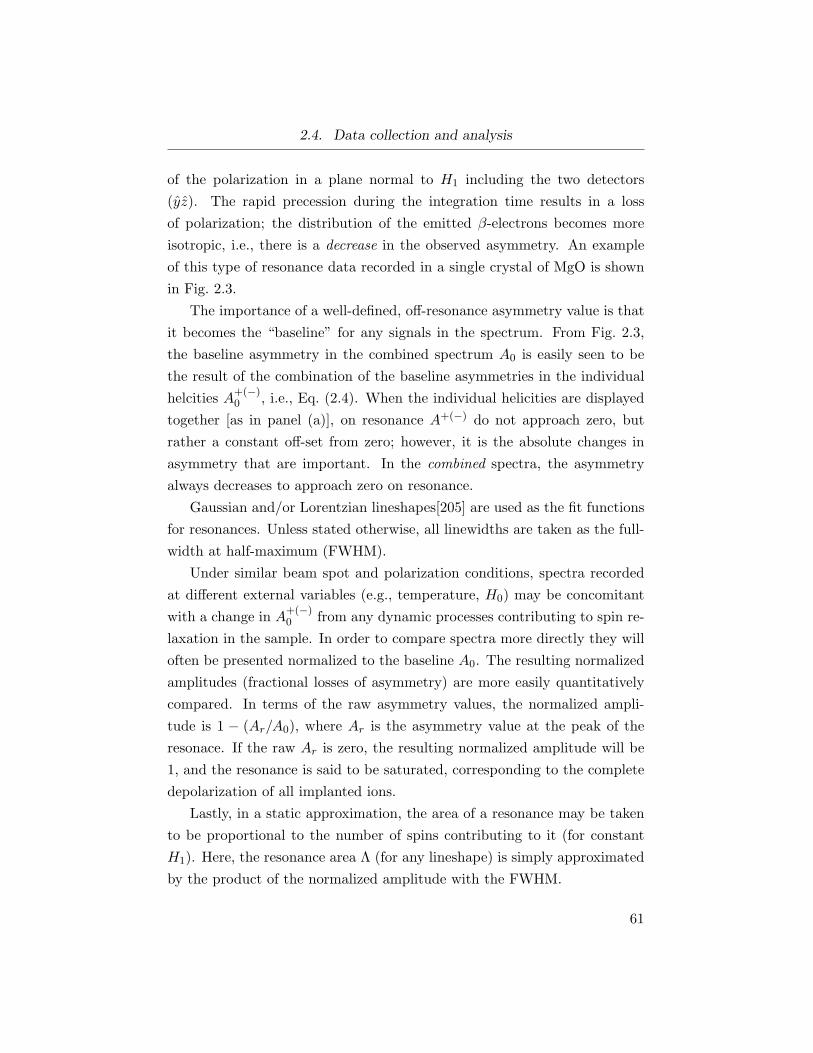
2.4. Data collection and analysis
of the polarization in a plane normal to H1 including the two detectors
(yz). The rapid precession during the integration time results in a loss
of polarization; the distribution of the emitted β-electrons becomes more
isotropic, i.e., there is a decrease in the observed asymmetry. An example
of this type of resonance data recorded in a single crystal of MgO is shown
in Fig. 2.3.
The importance of a well-defined, off-resonance asymmetry value is that
it becomes the “baseline” for any signals in the spectrum. From Fig. 2.3,
the baseline asymmetry in the combined spectrum A0 is easily seen to be
the result of the combination of the baseline asymmetries in the individual
helcities A+(−)0 , i.e., Eq. (2.4). When the individual helicities are displayed
together [as in panel (a)], on resonance A+(−) do not approach zero, but
rather a constant off-set from zero; however, it is the absolute changes in
asymmetry that are important. In the combined spectra, the asymmetry
always decreases to approach zero on resonance.
Gaussian and/or Lorentzian lineshapes[205] are used as the fit functions
for resonances. Unless stated otherwise, all linewidths are taken as the full-
width at half-maximum (FWHM).
Under similar beam spot and polarization conditions, spectra recorded
at different external variables (e.g., temperature, H0) may be concomitant
with a change in A+(−)0 from any dynamic processes contributing to spin re-
laxation in the sample. In order to compare spectra more directly they will
often be presented normalized to the baseline A0. The resulting normalized
amplitudes (fractional losses of asymmetry) are more easily quantitatively
compared. In terms of the raw asymmetry values, the normalized ampli-
tude is 1 − (Ar/A0), where Ar is the asymmetry value at the peak of the
resonace. If the raw Ar is zero, the resulting normalized amplitude will be
1, and the resonance is said to be saturated, corresponding to the complete
depolarization of all implanted ions.
Lastly, in a static approximation, the area of a resonance may be taken
to be proportional to the number of spins contributing to it (for constant
H1). Here, the resonance area Λ (for any lineshape) is simply approximated
by the product of the normalized amplitude with the FWHM.
61
2.4. Data collection and analysis
Figure 2.3: Representative resonance spectra recorded in a (100) crystalof MgO for H0 = 4 T at room temperature. Top panel shows the averagedspectra in the separate helicities and the bottom panel shows the spectrumafter combination.
62
2.4. Data collection and analysis
The beam spot is quite sensitive to instabilities throughout the beam
line, such as transient spikes in the voltages applied to electrostatic transport
elements, or small fluctuations in temperature at the Na vapourizer. These
can cause the beam spot to shift position on the sample during the collection
period of a cw-rf mode spectrum, i.e., multiple frequency scans in each
helicity generally requiring tens of minutes. Variations in the beam spot
on the sample may give rise to fluctuations in the polarization, introducing
significant noise or distortions into a spectrum, sometimes making it difficult
to define a flat off-resonance A0, or identify resonances of small amplitude.
2.4.2 Spin-lattice relaxation spectra
The spin-lattice relaxation rate T−11 ≡ λ is extracted from spectra that
monitor the polarization of the implated ions as a function of time in the
absence of the rf field. These time-differential spectra follow the same prin-
ciples of detection as those described above for resonances: The counts from
the two detectors can be used to generate an asymmetry that is directly pro-
portional to the Li nuclear polarization P (t). Again, spectra are recorded
in the individual helicities, then separate helicity spectra are averaged and
subsequently combined [Eqs. (2.3) and (2.4)].
The beam is introduced in short pulses of length δ. Fig. 2.4 shows an
example of these time spectra for δ = 0.5 s and δ = 4.0 s. Following the
beam pulse, a counting period of 10 s is used; however, in general, few Li
survive for longer than 8 s (making measurements of T1 ≫ τ difficult). This
cycle is repeated every 15 s until sufficient events are accumulated, typically
requiring 15–30 mins. A+(−)(t) is measured with a typical time resolution
of 10 ms. A pulsed beam is generated by the use of an electrostatic “kicker”
located near the target that deflects the beam either into the beam line or
to a beam dump. A pulse length of 4 s represents a balance between one
which is too short (δ = 0.5 s) or one which is unnecessarily long.
To fit data for δ = 4.0 s, a general spin relaxation function f(t, t′;λ) is as-
63
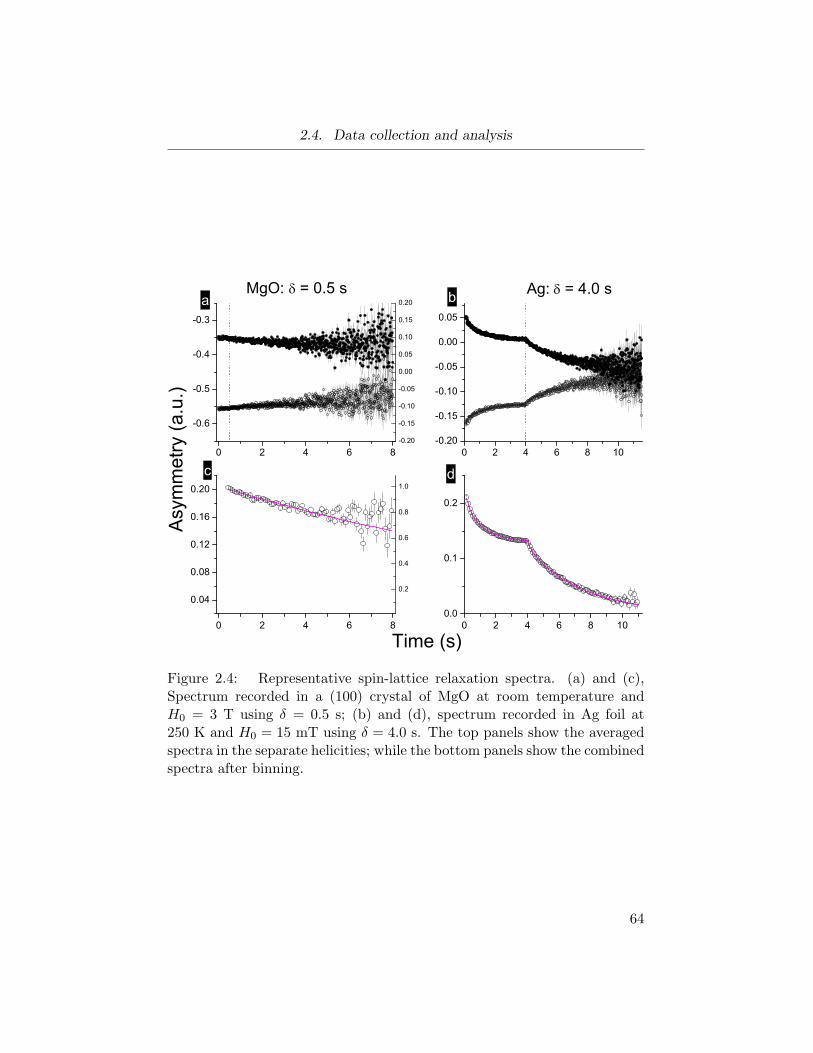
2.4. Data collection and analysis
Figure 2.4: Representative spin-lattice relaxation spectra. (a) and (c),Spectrum recorded in a (100) crystal of MgO at room temperature andH0 = 3 T using δ = 0.5 s; (b) and (d), spectrum recorded in Ag foil at250 K and H0 = 15 mT using δ = 4.0 s. The top panels show the averagedspectra in the separate helicities; while the bottom panels show the combinedspectra after binning.
64
2.4. Data collection and analysis
sumed for the ions implanted at t′, then the average polarization follows[206]
P (t) =
∫ t
0e−(t−t′)/τ f(t,t′;λ)dt′
∫ t
0e−t/τ dt
t ≤ δ
∫ δ
0e−(δ−t′)/τ f(t,t′;λ)dt′
∫ δ
0e−t/τ dt
t > δ.
(2.7)
One example of f(t, t′;λ) is the biexponential form[206],
f(t, t′;λ) = A1e−λ1(t−t′) +A2e
−λ2(t−t′). (2.8)
For instance, the Ag spectrum in Fig. 2.4(d) was fit using two components
according to the above two equations. The second component is a small
amplitude, faster relaxing one that is often needed to properly account for
T−11 data at short times in many materials.
In contrast, the MgO spectrum in Fig. 2.4(c) was fit to a single expo-
nentially relaxing component after the beam pulse only
A = Aδe−λ(t−δ), (2.9)
where Aδ is the asymmetry at the trailing edge of the beam pulse. The above
equation can also be generalized to multiple components; however, the MgO
spectrum shown could be fit satisfactorily to a single relaxing component.
Notice that the relaxation in MgO is slow (practically non-relaxing) even
at room temperature, as expected for a non-magnetic insulator with no
conduction electrons.
The combined spectra in panels (c) and (d) of Fig. 2.4 are presented after
the data in the time histograms has been further averaged. This process is
termed “binning,” and it mainly serves to ease in the visual inspection of the
spectra. An integer time factor is chosen over which the data is averaged. In
both spectra in question, this binning factor was 10; the A(t) data recorded
with 10 ms bins now appears in 100 ms bins (steps). Although seldom done,
binning can also be done for resonances where the averaging is done for the
asymmetry values over an interval of frequency. Clearly, this improves the
65
2.5. Additional considerations for resonance spectra
statistics per bin, but the resolution in time or frequency is compromised.
Care is always taken to choose a binning factor that is not too large, so as
to avoid “binning over” any fine structure in a spectrum.
2.5 Additional considerations for resonance
spectra
Here, some additional experimental details that are important to the inter-
pretation of resonance spectra are summarized.
2.5.1 Lineshapes and rf power-broadening
As mentioned above, Gaussian or Lorentzian lineshapes have been used to
fit the resonances obtained in the present β-NMR experiments. They are
both phenomenological, simple choices of lineshapes that can be used to
describe an absorption resonance.
In the absence of other broadening mechanisms, the line broadening in a
solid is dominated by the local magnetic field produced by the surrounding
nuclear magnetic dipoles. An expression for this broadening due to unlike
spins was given in Sec. 1.4 in Eq. (1.43) and is termed the van Vleck dipolar
linewidth. It is technically derived from consideration of the second mo-
ment of an absorption line due to magnetic broadening from unlike nuclear
spins, and is proportional to the width of a Gaussian lineshape. The second
moment of a Lorentzian lineshape is undefined. The Gaussian lineshape
is thus expected to describe a β-NMR resonance when the only source of
broadening is the local magnetic fields due to the host nuclear dipoles[161].
However, in the cw-mode employed here, larger amplitudes of H1 (i.e.,
Prf) leads to power-broadening of the resonances. This broadening is temperature-
independent (in contrast to the broadening due to dilute magnetic impuri-
ties). The broadening due to H1 gives rise to resonances that are better
described by Lorentzian lineshapes. This can be seen by transformation
into the rotating reference frame[20, 207], a frame rotating about z at the
rf frequency 2πν. Application of the H1 causes the spins to precess about
66
2.5. Additional considerations for resonance spectra
an effective field that is comprised of the now static H1 and a contribution
from H0. The applied rf is such that H1 is of azimuthal orientation in the
rotating frame; the spins are considered to be tipped through an angle φ by
the rf excitation. The effective field about which the spins precess can be
obtained from geometric considerations (cotφ) which yields the form of a
Lorentzian. The higher the rf power, the greater the width of the Lorentzian
γH1.
In the limit of low Prf , an approximation for including the contribution
from the power-broadening to a Gaussian lineshape is
σ2 ≈ σ20 + (γH1)2 + λ2, (2.10)
where σ0 is used to denote the intrinsic width from the host nuclear dipoles,
and λ = τ−1 + T−11 . For the metals studied here (i.e., Au and Pd) λ is
at least two orders of magnitude smaller than σ0. This point highlights an
important difference between present β-NMR measurements and the conven-
tional NMR of molecules in solution. In the latter case, the rapid motion
of the molecules leads to an averaging of local fields. In such cases, the
Fourier transform of the decay in pulsed NMR measurements will yield the
absorption resonance. The β-NMR resonances considered here cannot be
obtained through a Fourier transform of the spin-lattice relaxation signal.
The above equation is a means of approximating a small Lorentzian broad-
ening to a Gaussian lineshape. It is not rigorously valid when the width of
the Lorentzian component becomes comparable to the width of the Gaussian
component. In such cases, the lineshape becomes one which is a convolution
of a Gaussian with a Lorentzian, which is described by the Voigt function.
2.5.2 Demagnetization correction
In the previous Chapter, the relative frequency shift of the implanted Li
probes in metals was discussed as arising predominately from the coupling
to the conduction electrons, and as such is interpreted as the Knight shift.
Another contribution to this shift arises from the macroscopic demagnetizing
field that adds to the local field inside a magnetized material. This is a
67
2.5. Additional considerations for resonance spectra
classical field that originates from the surface of the sample, and hence is
geometry-dependent[21, 162]. For spherical samples, the demagnetization
contribution is exactly zero. Thus, in conventional NMR, shifts measured in
non-spherical samples can show an orientation dependence of the shift with
respect to H0[21], e.g., Ref. [208]. In terms of β-NMR in metal films, this
contribution to the Li shift is significant when the host metal has a large χ
(as in the case of Pd), or is ferromagnetic.
The demagnetization contribution is also approximately zero for thin
films when H0 is parallel to the plane of the film. However, for H0 normal
to the film plane, as in β-NMR, the demagnetization contribution is maxi-
mal. Correcting for the demagnetization can be done by noting the analogy
between this field and the depolarizing field effect on the local electric field
in a polarizable medium[3, 191]. The correction for thin film samples in
β-NMR is discussed in detail in Ref. [191].
The total local magnetic field Ht can be divided into four parts:
Htot = H0 +HD +HL +Hloc, (2.11)
where H0 is the applied field, HD the demagnetizing field, and HL the field
due to the Lorentz cavity. The field Hloc is the local field, taken as that
dominated by the immediate atomic neighbours of the site under consider-
ation, and is the quantity of interest. The Lorentz cavity is an imaginary
sphere (boundary) placed around an atom; the magnetization outside the
cavity can be treated in classical continuum theory, while that inside must
be treated atomically. Isolating the last three terms on the right-hand side
of the above equation and dividing by H0 gives,
(Htot −H0)/H0 = [(HD +HL)/H0] +Hloc/H0. (2.12)
In this equation, the left-hand side gives the observed relative shift, and
the second term on the right-hand side corresponds to the corrected shift
due only to the local contribution(s). By taking account of the quantity
(HD +HL)/H0, the measured shift can corrected.
68
2.5. Additional considerations for resonance spectra
In the following cgs units are used. For a spherical Lorentz cavity, HL =
4πM/3, while HD = −NM . Here M is the bulk magnetization, and N is
the dimensionless, geometry-dependent demagnetization factor that ranges
from 0 to 4π.10 By treating a thin film as an infinite slab with H0 normal
to the plane, N = 4π. Corrections to this value of N because of the finite
size of the sample are proportional to the thickness to lateral dimension
aspect ratio ξfilm. Samples for β-NMR are ∼ 1 cm2 and at most hundreds of
nanometers thick, thus ξfilm ∼ 10−5, and the corrections can be neglected.
Combining the above expressions yields
(HD +HL)/H0 = [−4π + (4π/3)]M/H0. (2.13)
Noting that M/H0 = χ, where specifically, it is χv the volume susceptibilty
of the host expressed in emu/cm3 that must be used. Substituting this result
into Eq. (2.12), the demagnetization-corrected Knight shift is given by:
Kc = K +8π
3χv. (2.14)
It is Kc that must be used when applying Eqs. (1.26) or (1.42) to extract
values of the hyperfine coupling constant or the Korringa ratio.
2.5.3 Quadrupole splitting
In the previous Chapter, the possible cubic stopping sites in the fcc lattice
were discussed and it was stated that at these sites, the EFG at the im-
planted probe is zero. In general, for stopping sites of non-cubic symmetry,
the EFG will be non-vanishing resulting in a quadrupole splitting of the
spectrum. The data of this thesis were all collected using large H0 where
the quadrupole interaction can be expected to be a perturbation on the Zee-
man interaction (as measured by νQ/νL ≪ 1). In this case, the quadrupole
interaction lifts the degneracy of the nuclear transitions— in particular for
β-NMR— the | ± 2〉 → | ± 1〉 transition.
As a consequence, facile identification of such quadrupolar resonances
100 to 1 in SI units.
69
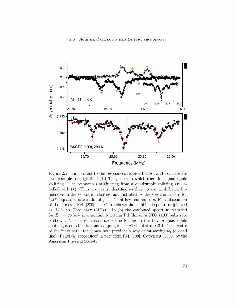
2.5. Additional considerations for resonance spectra
Figure 2.5: In contrast to the resonances recorded in Au and Pd, here aretwo examples of high field (4.1 T) spectra in which there is a quadrupolesplitting. The resonances originating from a quadrupole splitting are la-belled with (⋆). They are easily identified as they appear at different fre-quencies in the separate helicities, as illustrated by the spectrum in (a) for8Li+ implanted into a film of (bcc) Nb at low temperature. For a discussionof the sites see Ref. [209]. The inset shows the combined spectrum [plottedas A/A0 vs. Frequency (MHz)]. In (b) the combined spectrum recordedfor ELi = 28 keV in a nominally 50 nm Pd film on a STO (100) substrateis shown. The larger resonance is due to ions in the Pd. A quadrupolesplitting occurs for the ions stopping in the STO substrate[204]. The centreof the inner satellites shown here provides a way of estimating ν0 (dashedline). Panel (a) reproduced in part from Ref. [209]. Copyright (2009) by theAmerican Physical Society.
70
2.5. Additional considerations for resonance spectra
can be made through inspection of the spectra in the separate helicities. This
is illustrated by the spectrum recorded in a highly oriented Nb (110) film at
3 K shown in Fig. 2.5(a). The satellites that appear at different frequencies
in the opposite helicities can be assigned to ions stopping at a site with
a non-vanishing EFG and are marked by (⋆). In this example, the larger
amplitude resonance that appears at the same frequency in both helicities
is from ions stopping in an (essentially) cubic site. Upon combination of the
helicities [inset, Fig. 2.5(a)], the quadrupolar resonances contribute to a five
line spectrum from 8Li+ in two distinct sites[209].
Often crystalline SrTiO3 (STO) is employed as the substrate for thin
metal films in β-NMR. In particular, STO is well lattice-matched to Pd[210].
Quadrupole satellites are also seen in high H0 spectra for 8Li in STO, regard-
less of temperature[204]. As an example, a (combined) spectrum recorded
at full implantation energy in a nominally 50 nm Pd film deposited onto
a (100) single crystal of STO at 4.1 T is shown in Fig. 2.5(b). The inner
quadrupole satellites from ions in the STO are marked by (⋆), while the
larger resonance is from ions stopping in the metal layer. This spectrum
serves to illustrate that the centre of the satellites in STO can be used to
determine ν0. This highlights the use of substrates like STO or MgO as in
situ reference materials for the determination of the Knight shift. However,
comparison of Figs. 2.3(b) and 2.5(b) illustrates that MgO is the preferable
substrate for this purpose, as the centre of the quadrupole satellites from
STO is less precisely determined.
Inspection of Fig. 2.5 shows, for a given helicity, the size of the quadrupole
splitting determined by νQ is tens of kHz in Nb, and hundreds of kHz in
STO, but in both cases νQ/νL ≪ 1, so the quadrupole interaction can in-
deed be treated as a first-order perturbation on the Zeeman interaction, i.e.,
the “high-field limit.”
With this summary of the technical details completed, the results of 8Li
β-NMR of gold and palladium will now be discussed in turn.
71
Chapter 3
β-NMR of 8Li in Gold
3.1 Introduction
The application of low energy 8Li β-NMR to study the electronic and mag-
netic properties of multilayers and heterostructures requires an understand-
ing of the behaviour of the probe in simple materials. Such investigations
also assist in the overall development of the technique. The Pauli spin
susceptibility of the group 11 metals (Cu, Ag, Au) is not temperature-
dependent. Thus, the behaviour of 8Li in these simpler metals can be con-
trasted with the results presented later for 8Li in Pd.
In the Introduction the use of thin metal overlayers for proximal magne-
tometry experiments was discussed. The inertness and high density of Au
make it an attractive candidate for such experiments, and as a thin protec-
tive capping layer, it may also serve as an in situ reference for Knight shift
measurements (for samples where no magnetic coupling is to be expected).
An important prerequisite is to establish the behaviour of 8Li in bulk Au. An
initial β-NMR study of 8Li in Au found two resonances with temperature-
dependent amplitudes[211], very similar to results from Ag[184]. In this
Chapter, significantly more details of the behaviour of 8Li in Au are pre-
sented. A comparison of the hyperfine coupling constants for 8Li in Au is
made with previously reported results for this probe in the other two group
11 metals, Ag[184] and Cu[185], and in Al[186].
3.2 Results
Data is presented from measurements on two distinct samples of Au to
verify that the results are intrinsic. The first is a 100 nm film deposited on a
72
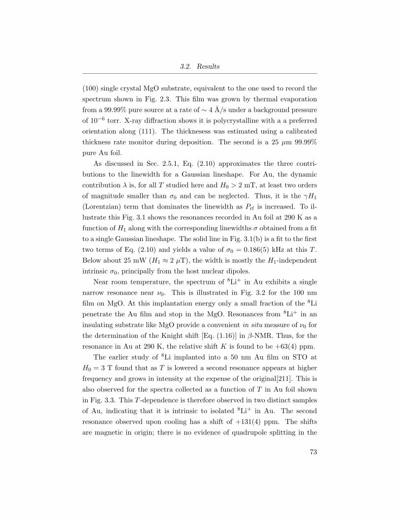
3.2. Results
(100) single crystal MgO substrate, equivalent to the one used to record the
spectrum shown in Fig. 2.3. This film was grown by thermal evaporation
from a 99.99% pure source at a rate of ∼ 4 A/s under a background pressure
of 10−6 torr. X-ray diffraction shows it is polycrystalline with a a preferred
orientation along (111). The thicknesess was estimated using a calibrated
thickness rate monitor during deposition. The second is a 25 µm 99.99%
pure Au foil.
As discussed in Sec. 2.5.1, Eq. (2.10) approximates the three contri-
butions to the linewidth for a Gaussian lineshape. For Au, the dynamic
contribution λ is, for all T studied here and H0 > 2 mT, at least two orders
of magnitude smaller than σ0 and can be neglected. Thus, it is the γH1
(Lorentzian) term that dominates the linewidth as Prf is increased. To il-
lustrate this Fig. 3.1 shows the resonances recorded in Au foil at 290 K as a
function of H1 along with the corresponding linewidths σ obtained from a fit
to a single Gaussian lineshape. The solid line in Fig. 3.1(b) is a fit to the first
two terms of Eq. (2.10) and yields a value of σ0 = 0.186(5) kHz at this T .
Below about 25 mW (H1 ≈ 2 µT), the width is mostly the H1-independent
intrinsic σ0, principally from the host nuclear dipoles.
Near room temperature, the spectrum of 8Li+ in Au exhibits a single
narrow resonance near ν0. This is illustrated in Fig. 3.2 for the 100 nm
film on MgO. At this implantation energy only a small fraction of the 8Li
penetrate the Au film and stop in the MgO. Resonances from 8Li+ in an
insulating substrate like MgO provide a convenient in situ measure of ν0 for
the determination of the Knight shift [Eq. (1.16)] in β-NMR. Thus, for the
resonance in Au at 290 K, the relative shift K is found to be +63(4) ppm.
The earlier study of 8Li implanted into a 50 nm Au film on STO at
H0 = 3 T found that as T is lowered a second resonance appears at higher
frequency and grows in intensity at the expense of the original[211]. This is
also observed for the spectra collected as a function of T in Au foil shown
in Fig. 3.3. This T -dependence is therefore observed in two distinct samples
of Au, indicating that it is intrinsic to isolated 8Li+ in Au. The second
resonance observed upon cooling has a shift of +131(4) ppm. The shifts
are magnetic in origin; there is no evidence of quadrupole splitting in the
73
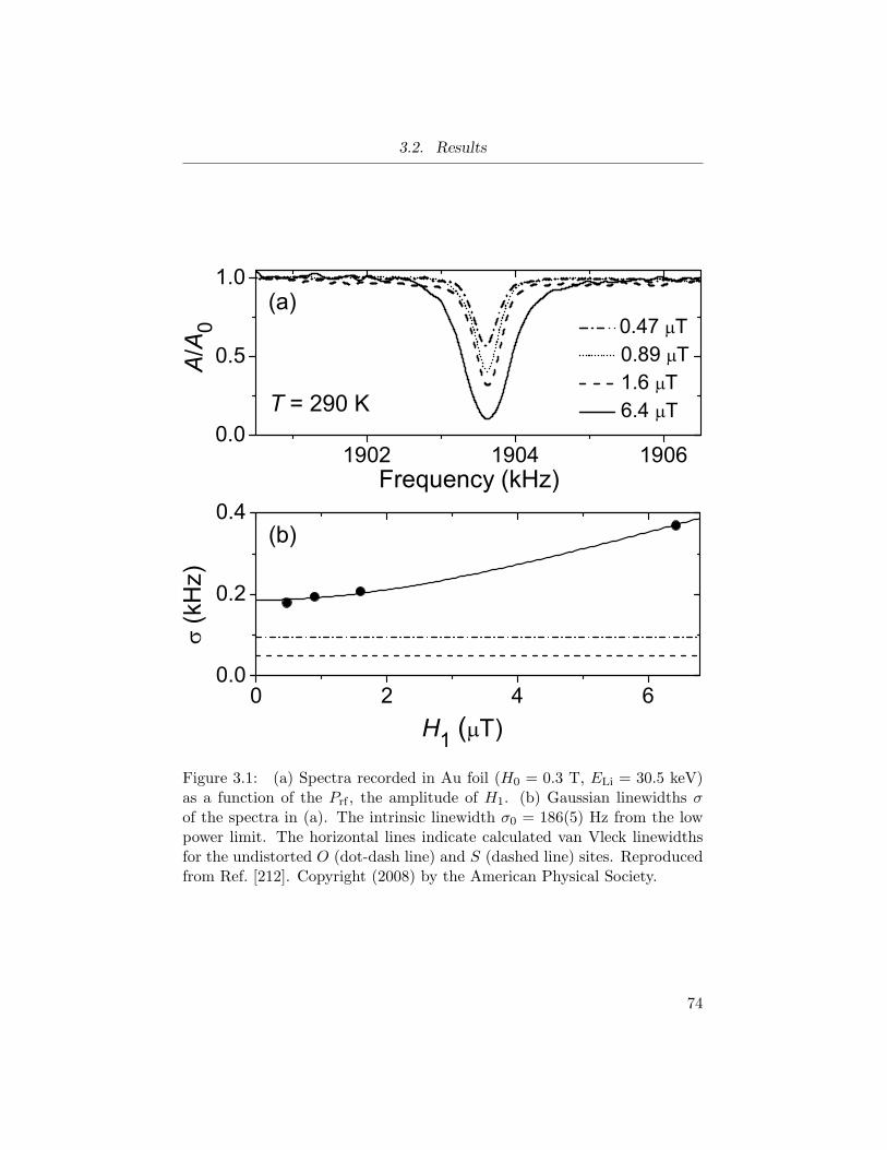
3.2. Results
Figure 3.1: (a) Spectra recorded in Au foil (H0 = 0.3 T, ELi = 30.5 keV)as a function of the Prf , the amplitude of H1. (b) Gaussian linewidths σof the spectra in (a). The intrinsic linewidth σ0 = 186(5) Hz from the lowpower limit. The horizontal lines indicate calculated van Vleck linewidthsfor the undistorted O (dot-dash line) and S (dashed line) sites. Reproducedfrom Ref. [212]. Copyright (2008) by the American Physical Society.
74
3.2. Results
Figure 3.2: Typical high field spectra of 8Li+ implanted into 100 nmAu/MgO (H1 ∼ 3 µT) showing the large resonance in Au and its Knight shiftrelative to the resonance in MgO. Each spectrum is fit to two Lorentzians.Reproduced in part from Ref. [212]. Copyright (2008) by the AmericanPhysical Society.
75
3.2. Results
separate helicities. By analogy with the behaviour of (i) the T -dependence of
the resonances and (ii) the relative magnitudes of K in the other group 11 fcc
metals[184, 185], the resonances in Au are provisionally assigned to ions in
the octahedral interstitial O site (high frequency line), and the substitutional
S site (lower frequency line). These spectra were recorded with H1 ∼ 5
µT and are found to fit well to Lorentzian lineshapes due to the rf power-
broadening; cf. Fig. 3.1(b). From these fits, the T -dependence of K, the
linewidths (FWHM), and the normalized amplitudes are given in Fig. 3.4.
The shifts are T -independent, consistent with Knight shifts. The linewidths
are relatively constant with T , with the O line slightly broader than the S
line. It is noted that the S widths agree fairly well with the full width (2σ)
obtained from the fit in Fig. 3.1(b) for H1 = 5 µT.
The amplitudes of the two resonances show a cross-over centred at T ≈200 K, a somewhat higher temperature than the similar cross-over observed
in Ag[184] (≈ 150 K), and much higher than the one observed in Cu[185]
(≈ 50 K). As the temperature is further decreased below about 50 K, the
narrow O resonance is observed to decrease in amplitude; a similar reduction
of the O resonance is seen in Cu[185], but not in Ag[184].
To investigate the possible depth-dependence of the resonances from e.g.,
a near-surface effect, spectra were collected for several incident energies cor-
responding to mean implantation depths of 10 to 95 nm, according to the
TRIM.SP simulations (see Appendix B). No significant depth dependence
of either signal (e.g., width, position) is observed. Spectra recorded in the
film at 4.1 T and room temperature for ELi = 13 keV and ELi = 28 keV
are compared in Fig. 3.2. At 13 keV essentially no ions should be implanted
into the substrate (cf. Fig. B.1), yet a signal from Li in the MgO is still
observed, although of reduced amplitude. This is expected as a small area
of two diagonal corners of the substrate were masked during the film depo-
sition and remain uncovered by the Au. This indicates the beam spot was
not entirely focussed on the Au. At this T , the spectrum is dominated by
the signal from ions in the S sites. From Lorentzian fits to the spectra, the
linewidths and K for this site are not appreciably different despite ELi, and
thus R, differing by a factor of 2.
76
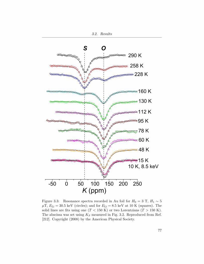
3.2. Results
Figure 3.3: Resonance spectra recorded in Au foil for H0 = 3 T, H1 ∼ 5µT, ELi = 30.5 keV (circles); and for ELi = 8.5 keV at 10 K (squares). Thesolid lines are fits using one (T < 150 K) or two Lorentzians (T > 150 K).The abscissa was set using KS measured in Fig. 3.2. Reproduced from Ref.[212]. Copyright (2008) by the American Physical Society.
77
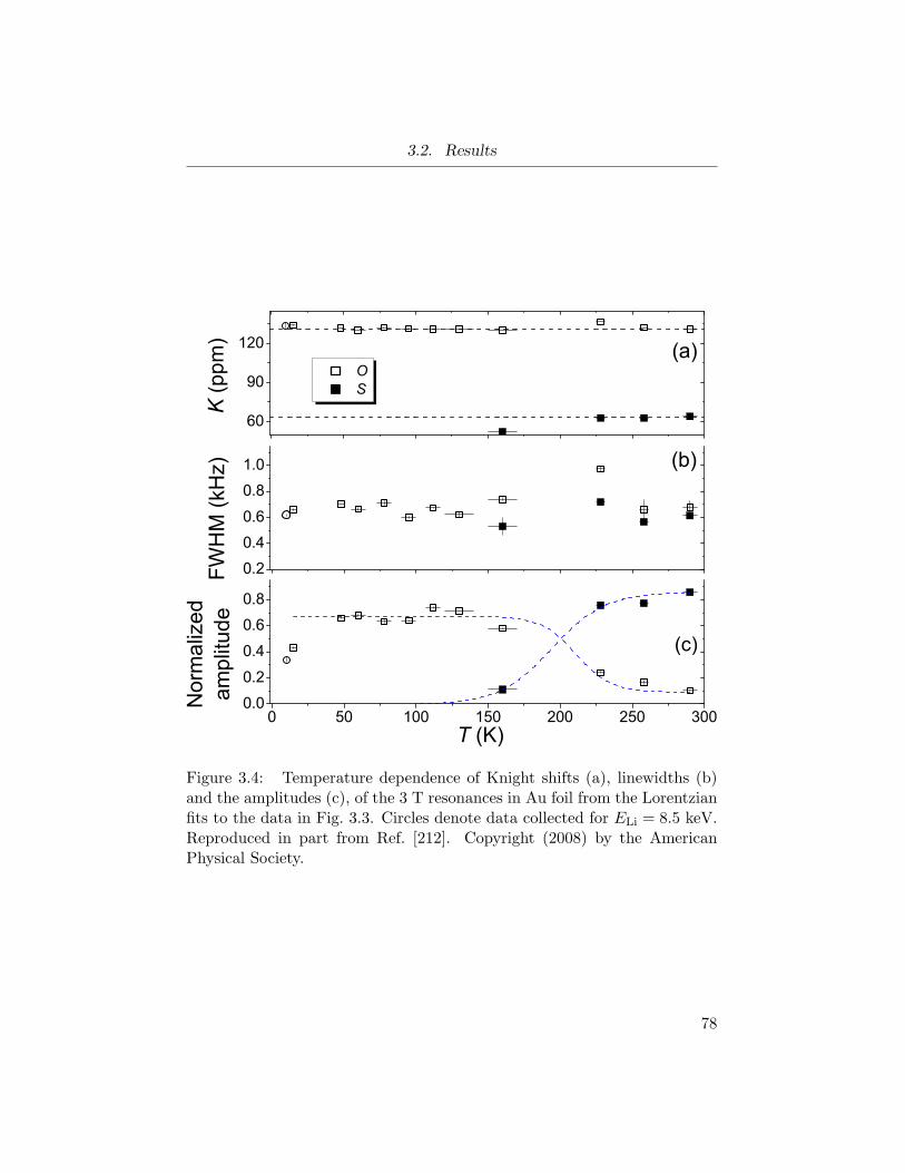
3.2. Results
Figure 3.4: Temperature dependence of Knight shifts (a), linewidths (b)and the amplitudes (c), of the 3 T resonances in Au foil from the Lorentzianfits to the data in Fig. 3.3. Circles denote data collected for ELi = 8.5 keV.Reproduced in part from Ref. [212]. Copyright (2008) by the AmericanPhysical Society.
78
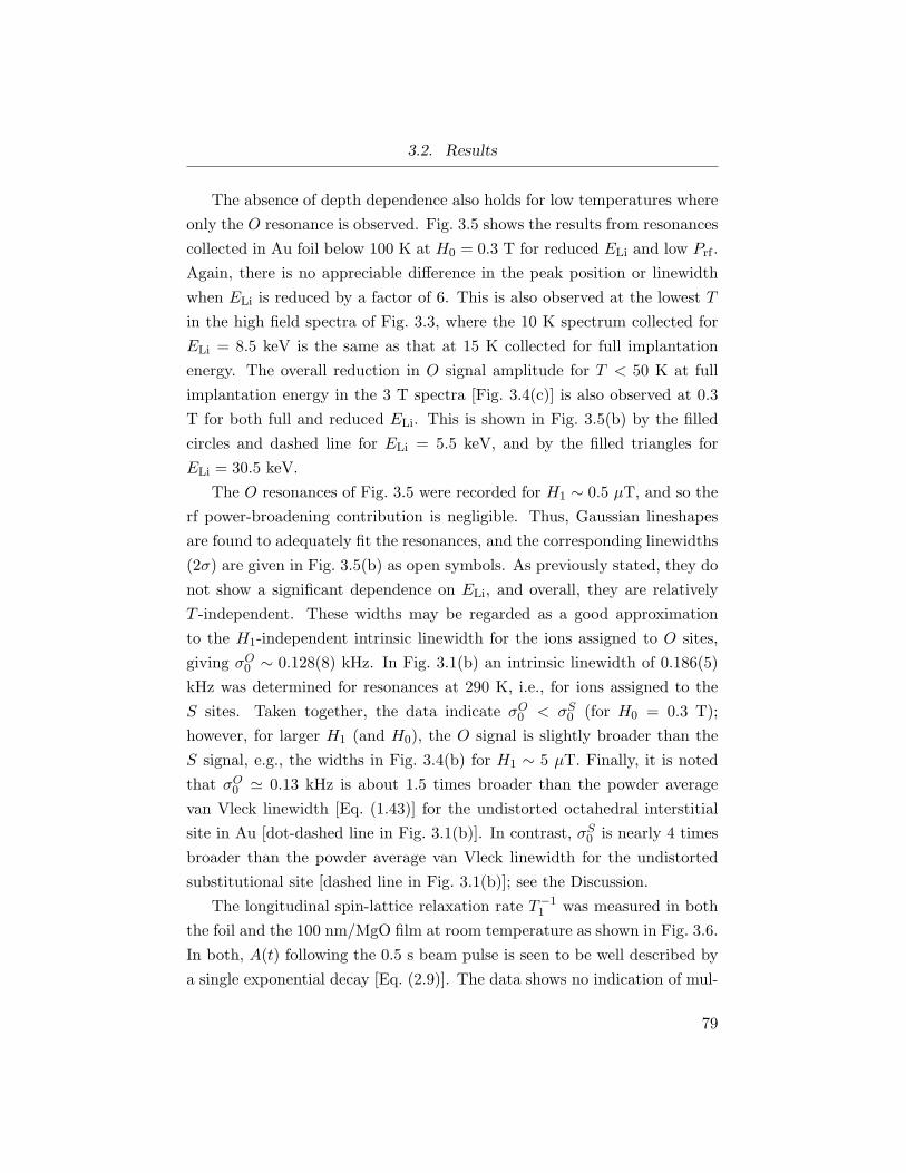
3.2. Results
The absence of depth dependence also holds for low temperatures where
only the O resonance is observed. Fig. 3.5 shows the results from resonances
collected in Au foil below 100 K at H0 = 0.3 T for reduced ELi and low Prf .
Again, there is no appreciable difference in the peak position or linewidth
when ELi is reduced by a factor of 6. This is also observed at the lowest T
in the high field spectra of Fig. 3.3, where the 10 K spectrum collected for
ELi = 8.5 keV is the same as that at 15 K collected for full implantation
energy. The overall reduction in O signal amplitude for T < 50 K at full
implantation energy in the 3 T spectra [Fig. 3.4(c)] is also observed at 0.3
T for both full and reduced ELi. This is shown in Fig. 3.5(b) by the filled
circles and dashed line for ELi = 5.5 keV, and by the filled triangles for
ELi = 30.5 keV.
The O resonances of Fig. 3.5 were recorded for H1 ∼ 0.5 µT, and so the
rf power-broadening contribution is negligible. Thus, Gaussian lineshapes
are found to adequately fit the resonances, and the corresponding linewidths
(2σ) are given in Fig. 3.5(b) as open symbols. As previously stated, they do
not show a significant dependence on ELi, and overall, they are relatively
T -independent. These widths may be regarded as a good approximation
to the H1-independent intrinsic linewidth for the ions assigned to O sites,
giving σO0 ∼ 0.128(8) kHz. In Fig. 3.1(b) an intrinsic linewidth of 0.186(5)
kHz was determined for resonances at 290 K, i.e., for ions assigned to the
S sites. Taken together, the data indicate σO0 < σS
0 (for H0 = 0.3 T);
however, for larger H1 (and H0), the O signal is slightly broader than the
S signal, e.g., the widths in Fig. 3.4(b) for H1 ∼ 5 µT. Finally, it is noted
that σO0 ≃ 0.13 kHz is about 1.5 times broader than the powder average
van Vleck linewidth [Eq. (1.43)] for the undistorted octahedral interstitial
site in Au [dot-dashed line in Fig. 3.1(b)]. In contrast, σS0 is nearly 4 times
broader than the powder average van Vleck linewidth for the undistorted
substitutional site [dashed line in Fig. 3.1(b)]; see the Discussion.
The longitudinal spin-lattice relaxation rate T−11 was measured in both
the foil and the 100 nm/MgO film at room temperature as shown in Fig. 3.6.
In both, A(t) following the 0.5 s beam pulse is seen to be well described by
a single exponential decay [Eq. (2.9)]. The data shows no indication of mul-
79
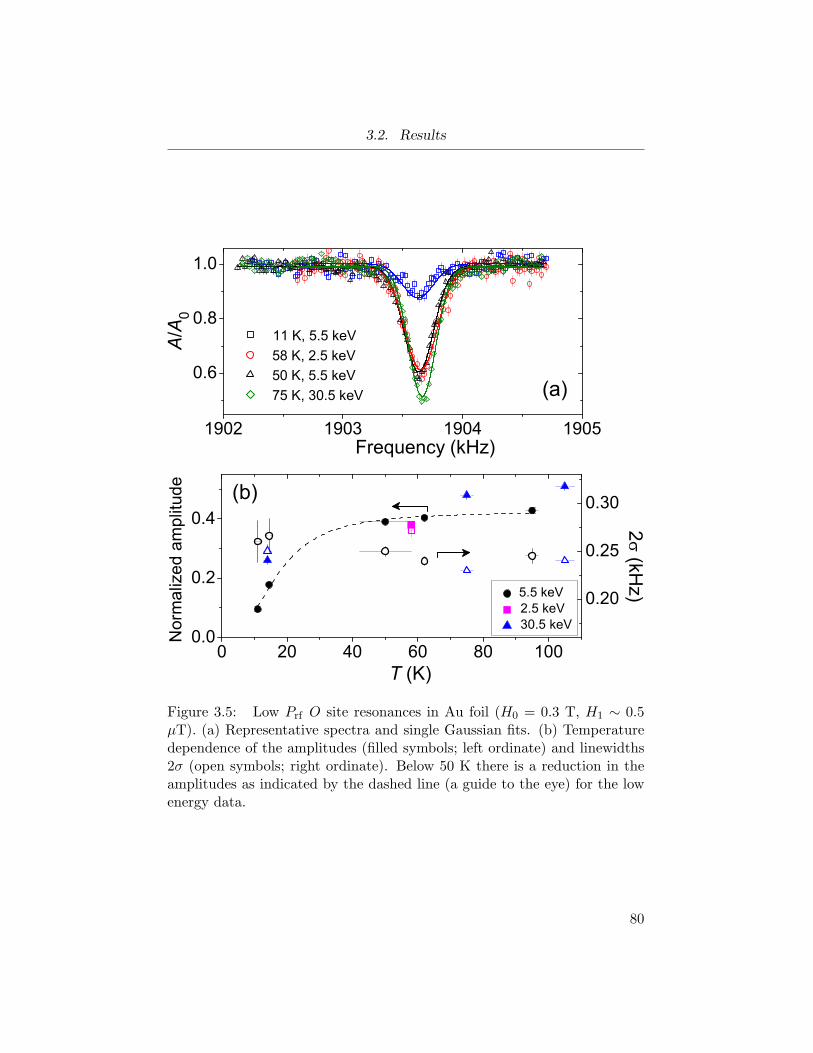
3.2. Results
Figure 3.5: Low Prf O site resonances in Au foil (H0 = 0.3 T, H1 ∼ 0.5µT). (a) Representative spectra and single Gaussian fits. (b) Temperaturedependence of the amplitudes (filled symbols; left ordinate) and linewidths2σ (open symbols; right ordinate). Below 50 K there is a reduction in theamplitudes as indicated by the dashed line (a guide to the eye) for the lowenergy data.
80
3.3. Discussion
tiple relaxing components[213], consistent with the absence of quadrupole
splitting in the spectra and the assignment of the ions to the cubic S sites.
For the 100 nm film spectrum, ELi = 13 keV, and as discussed above, the
fraction of ions penetrating into the MgO substrate is negligible. However,
as illustrated in Fig. 2.4(c), the relaxation rate in MgO is 2.6 times slower, so
the small fraction of Li that may stop in exposed corners of the substrate are
neglected (i.e., a small, non-relaxing background). The agreement between
the two samples is quite good, indicating there is no sample dependence.
The average of the two rates, T−11 = 0.127(7) s−1, is taken as the field-
independent (Korringa) rate at this temperature.
3.3 Discussion
To begin, the similarities in the temperature dependence of the resonances
of 8Li+ in Au and Ag are noted. In both metals, at high field, two narrow
resonances, positively shifted from νL with nearly T -independent positions,
but strongly T -dependent amplitudes are observed [cf. Fig. 1.3(b)]. This
is also found for 8Li in polycrystalline Cu, but in this case the resonances
are broad and not well resolved[185]. This is due to the order-of-magnitude
larger γ of the two Cu isotopes giving rise to much larger dipolar linewidths;
similar unresolved lines are observed for 8Li in Al[186]. The two resonances
have been provisionally assigned to ions stopping in two inequivalent cubic
sites of the host lattice. Specifically, for all three metals the high tempera-
ture (smaller K) line is attributed to ions in the substitutional S site, and
the low temperature (larger K) line to those in the octahedral interstitial O
site. This is reasonable, simply based on the relative sizes of the three cubic
sites in the fcc lattice (S > O > T ). These assignments are motivated by
analogy to results from 12B cross-relaxation in Cu[179, 182]. Further, the
site assignments in the group 11 metal hosts are corroborated by the recent
measurements[172] and calculations[171] for 8Li in isostructural Ni. In this
picture, the T -dependent resonance amplitudes result from the thermally-
activated O → S site transition, since the smaller O site is metastable and
the larger S site is a lower energy configuration for the ions. In Au, the
81
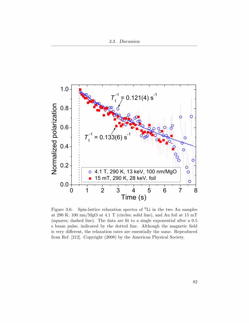
3.3. Discussion
Figure 3.6: Spin-lattice relaxation spectra of 8Li in the two Au samplesat 290 K: 100 nm/MgO at 4.1 T (circles; solid line), and Au foil at 15 mT(squares; dashed line). The data are fit to a single exponential after a 0.5s beam pulse, indicated by the dotted line. Although the magnetic fieldis very different, the relaxation rates are essentially the same. Reproducedfrom Ref. [212]. Copyright (2008) by the American Physical Society.
82
3.3. Discussion
ions evidently have sufficient thermal energy for this migration (within the
lifetime of the Li) for T above ≈ 150 K. Recall, from the discussion in Chap-
ter 1 that this site transition may be related to the onset of mobility of the
vacancies created during the athermal implantion of the probes. Although
these defects are known to become mobile typically at higher temperatures
(known as stage III annealing[188]), the ion implantation process may lower
the energy barrier to their mobility. Note from Fig. 3.4(b) that, for the
temperatures bracketing the region of this site change, the linewidths show
no indication of motional narrowing.
The dipolar linewidth is site-dependent, but uncertainty in the extent
of local lattice distortion (relaxation) around the implanted 8Li makes it
difficult to use for definitive site assignments. However, such calculations are
in reasonable agreement[180, 214] with the assignments for light, beta-active
ions implanted in Cu. Because of the small 197Au nuclear moment, small
dipolar widths are expected. Indeed, it is only because they are small that
such closely spaced resonances can be resolved, in contrast to the cases of
Cu and Al mentioned above. The widths of the narrow 8Li resonances in Au
are larger than the dipolar (van Vleck) widths calculated for an undistorted
lattice [Fig. 3.1(b)].
The origin of the additional linewidth is not clear. For example, the
widths in Fig. 3.4(b) show no temperature dependence and are similar for
both S and O resonances, thus they are not due to residual (ppm level)
magnetic impurities in the Au, which would yield temperature- (and field-)
dependent widths. The broadening likely arises from a local distortion of the
Au lattice about the 8Li as the dipolar width is dominated by the contribu-
tion from the nearest neighbours. A decrease of the distance to the nearest
neighbour Au dipoles would increase the dipolar width. This possibility has
been reported for other implanted probes, e.g., 12B in ZnSe[177]. Alterna-
tively, the linewidth may reflect a contribution from a narrow, unresolved
quadrupolar powder pattern if the 8Li site is not perfectly cubic. Slightly
noncubic sites (with associated EFGs) could result from a small, symmetry-
breaking, local lattice distortion caused by the 8Li or, as has been suggested
for 12B in fcc metals[180], the EFG from close-by point defects created dur-
83
3.3. Discussion
ing the implantation of the probe (see Appendix B).
The finding that σO0 < σS
0 (at 0.3 T) is opposite to what is expected on
the basis of the calculated dipolar widths in Fig. 3.1(b) of 0.095 kHz for the
undistorted O sites, and 0.049 kHz for the undistorted S sites. This situa-
tion perhaps arises from opposite local host lattice relaxations surrounding
the Li ions at each site, as reported for 12B in Cu[179]: a local contraction
about ions in S sites causing increased linewidths, and a local expansion of
the lattice about ions in O sites, as σO0 is just slightly broader than the cal-
culated van Vleck width, yet narrower in comparison to σS0 . This scenario
is based on measurements at a single H0. At 3 T and for larger H1, the O
resonances are slightly broader than the S resonances [Fig. 3.4(b)]. The H1-
independent intrinsic linewidths may be H0-dependent and this dependence
may be different for each site[176, 177]. As mentioned in the Introduc-
tion this arises because the implanted ions act as charged impurities that
create EFGs sensed by the host nuclei potentially influencing their dipolar
fields[176]. Thus, a detailed knowledge of σ0 of either site awaits measure-
ments at various external fields. For the remainder of this discussion, it will
be assumed that these site assignments are correct, noting that most of the
comparisons will not be drastically altered if another subset of the three
cubic sites is chosen (the major difference being the coordination of the site
z).
For T < 50 K there is a reduction in the O resonance amplitude. Prelim-
inary data strongly suggests that this reduction is due to a small fraction of
ions associated with implantation-created defects that cause a quadrupolar
broadening which cannot be resolved for the amplitudes of H1 employed for
the present measurements.
The raw Knight shifts are corrected for the contribution due to demag-
netization using Eq. (2.14) for χP = 1.21 × 10⁻⁶ emu/cm3[21], yielding the
corrected shifts KcO = +141(4) ppm and Kc
S = +73(5) ppm— overall small
corrections. The ratio of the shifts for the two sites is then KcO/K
cS ∼ 2,
corresponding to a splitting of 68(6) ppm. As χP for Au is T -independent,
the shifts are likewise in the range of 10–290 K [Fig. 3.4(a)]. The splitting
between the S and O lines observed in the polycrystalline Au foil is the same
84
3.3. Discussion
as that measured previously in a more highly oriented 50 nm film[211], in-
dicating that K, and thus Ahf , is predominantly isotropic, as expected for a
cubic host. The site-dependence of the shift is attributed to different hyper-
fine coupling constants as a result of hybridization of the 8Li+ 2s orbital with
the host s band, i.e., 2s − 6s hybridization. Using Eq. (1.42), AShf = 2.8(2)
kG/µB (z = 12), and AOhf = 10.7(3) kG/µB (z = 6).
These values are compared to those for 8Li in the other simple metals
in Table 3.1. For a given site, Ahf varies by no more than a factor of
2. The origin of the difference in Ahf between different hosts depends on
details of the local electronic structure. As discussed in Chap. 1, Ahf is
sensitive to several factors like the band structure of the host, the local
electronic screening, and the extent of lattice relaxation around the probe.
The strength of the hybridization is, in the simplest picture, a function of
z and the distance between the probe and the neighbouring host atoms.
Comparing the O site, z is half as big, but the distance to the nearest
neighbours is less. If this were the only consideration, similarAhfs for Au and
Ag would be expected, on the basis that the lattice constants are essentially
the same, instead the coupling constants for Au are about half the values
for Ag (and χP for these two metals only differs by about 20%). Table 3.1
also lists the ratio AOhf/A
Shf , which is found to be similar for all three metals,
although it is slightly larger for Au than Ag and Cu, in accordance with the
trend in the lattice constants (Cu<Ag≈Au). First-principles calculations for
a nonmagnetic defect in a nonmagnetic host, like 8Li in these three metals,
would be very useful to compare with the results of β-NMR.
At high fields, the T−11 is dominated by the Korringa mechanism. At
room T , T−11 of 8Li in Ag[184] and Cu[185] is nearly 3 times faster than in Au.
The present, average room T relaxation time in Au (Fig. 3.6), T1 = 7.9(4)
s, is half the 17(3) s reported by Koenig et al.[189], but double the 4(1)
s measured by Haskell and Madansky[166]. It is within the range of the
reported times, but the origin of the discrepancy is not certain, especially
since previous results differ from each other by a factor of 4. In light of
the sample-independence seen in Fig. 3.6, it is concluded that the present
value of 7.9(4) s is the most reliable to date for 8Li in Au. The authors of
85
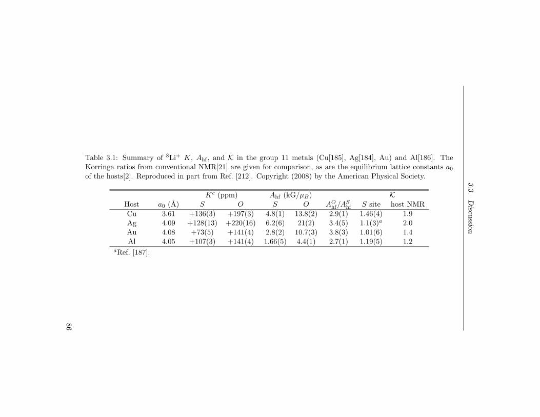
3.3
.D
iscussio
n
Table 3.1: Summary of 8Li+ K, Ahf , and K in the group 11 metals (Cu[185], Ag[184], Au) and Al[186]. TheKorringa ratios from conventional NMR[21] are given for comparison, as are the equilibrium lattice constants a0
of the hosts[2]. Reproduced in part from Ref. [212]. Copyright (2008) by the American Physical Society.
Kc (ppm) Ahf (kG/µB) KHost a0 (A) S O S O AO
hf/AShf S site host NMR
Cu 3.61 +136(3) +197(3) 4.8(1) 13.8(2) 2.9(1) 1.46(4) 1.9Ag 4.09 +128(13) +220(16) 6.2(6) 21(2) 3.4(5) 1.1(3)a 2.0Au 4.08 +73(5) +141(4) 2.8(2) 10.7(3) 3.8(3) 1.01(6) 1.4Al 4.05 +107(3) +141(4) 1.66(5) 4.4(1) 2.7(1) 1.19(5) 1.2
aRef. [187].
86
3.3. Discussion
Ref. [189] note that in both of the previous studies (using MeV recoil ions)
the temperature of the Au samples was not controlled during irradiation;
however, they conclude that contamination of the sample surface was the
most likely reason for the faster 4(1) s relaxation time reported in the earliest
study. A relaxation time of 3.3(3) s is also reported in Ref. [189] for 8Li in
Ag foil at room T , which agrees very well with measurements using the
TRIUMF β-NMR spectrometer for 8Li in a Ag film.[184]. Determination
of relaxation times that are significantly longer than the probe lifetime τ
is difficult. The present measurement using 8Li+ polarized in two helicities
accurately determines the baseline corresponding to the thermal equilibrium
polarization, even though the relaxation is too slow to reach this value during
the experiment.
The average T−11 value can be combined with Kc
S in Eq. (1.26) to yield
K = 1.01(6) for 8Li in Au at 290 K. This result is remarkably close to the
ideal value of 1, and as will be shown in the following chapters, very different
from that measured in a strongly enhanced metal like Pd. The K values for
the simple metal hosts are given in Table 3.1. They all reveal reductions in
enhancement for 8Li in comparison to the host nuclei (conducted at cryo-
genic temperatures to improve signal-to-noise). The “disenhancement” is
largest for Ag. The KAu is slightly larger (or similar to11) that for the 8Li
probe. Ions in S sites should have approximately the same spatial Fourier
transform Ahf(q) as the host nuclei. It can be concluded that the presence
of the 8Li+ does not strongly influence K, e.g., via electron scattering. A
study comparing K measured for 12B in the group 11 metals (assigned to O
sites) with that of the host nuclei found near equal values for Cu and Ag,
but a larger enhancement for Au[173]. The possibility was suggested that
this “Au anomaly” was specific to that probe[173]. The lack of enhancement
for 8Li in Au supports that proposal.
11Preliminary results from T−11 measurements in Au foil as a function of temperature
at 15 mT suggest KS ∼ 1.2, and KO ∼ 1.4.
87
3.4. Conclusions
3.4 Conclusions
To summarize the β-NMR has been used to study the behaviour of low
energy 8Li+ implanted in bulk Au. Two narrow resonances corresponding
to two cubic stopping sites are found. These are assigned to 8Li ions in
the octahedral interstitial O, and substitutional S sites. As expected for
a simple metal, the Knight shifts for ions in these sites are independent
of temperature, as are the resonance linewidths. A transition from the
metastable O site to the S site is observed centred at about 190 K. Values
for the intrinsic linewidths of the two resonances are also reported, with
both being broader than the van Vleck width for the undistorted sites, with
the additional width being greater for the S site. No evidence for a depth
dependence to these narrow resonances is found for implantation depths in
the range of 10–95 nm. The spectra in Au are very similar to those in Ag,
but with smaller shifts, and a considerably slower spin-lattice relaxation rate
for the S site. The Korringa ratio for S site ions in Au is not significantly
enhanced above the free electron gas value of one, and is also not very
different from the value obtained from Au NMR. K for substitutional 8Li
in the other simple metals also shows no significant enhancement over the
respective host values; instead, there is a disenhancement in Cu and in Ag
that is greater than in Au.
The T−11 is found to be highly field-independent for external fields greater
than at least 15 mT at 290 K.
Overall, the data show that 8Li probes the intrinsic electronic structure
of Au, and the behaviour of the probe in this host is quite similar to that
in the other simple metals. The results of 8Li β-NMR of Au are straight-
forwardly interpreted making this metal an excellent candidate for future
β-NMR studies of, e.g., magnetic multilayer heterostructures.
88
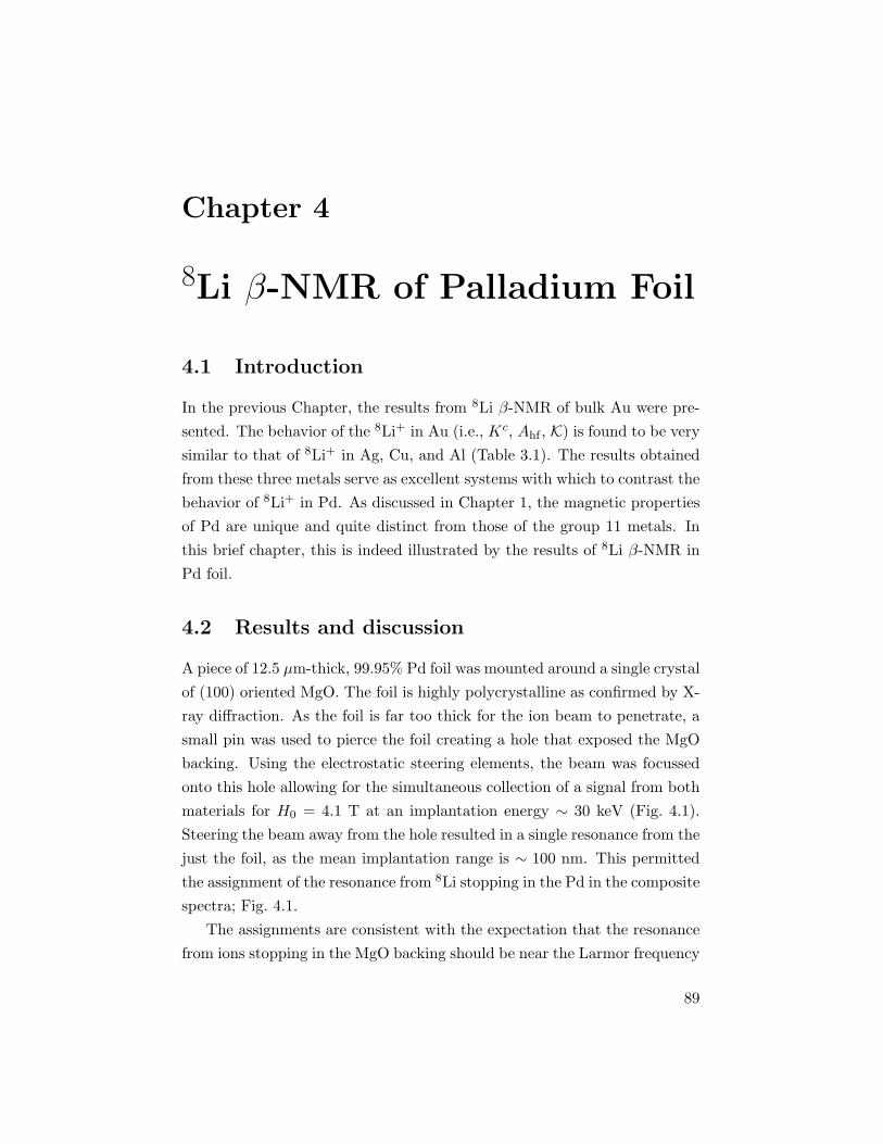
Chapter 4
8Li β-NMR of Palladium Foil
4.1 Introduction
In the previous Chapter, the results from 8Li β-NMR of bulk Au were pre-
sented. The behavior of the 8Li+ in Au (i.e., Kc, Ahf , K) is found to be very
similar to that of 8Li+ in Ag, Cu, and Al (Table 3.1). The results obtained
from these three metals serve as excellent systems with which to contrast the
behavior of 8Li+ in Pd. As discussed in Chapter 1, the magnetic properties
of Pd are unique and quite distinct from those of the group 11 metals. In
this brief chapter, this is indeed illustrated by the results of 8Li β-NMR in
Pd foil.
4.2 Results and discussion
A piece of 12.5 µm-thick, 99.95% Pd foil was mounted around a single crystal
of (100) oriented MgO. The foil is highly polycrystalline as confirmed by X-
ray diffraction. As the foil is far too thick for the ion beam to penetrate, a
small pin was used to pierce the foil creating a hole that exposed the MgO
backing. Using the electrostatic steering elements, the beam was focussed
onto this hole allowing for the simultaneous collection of a signal from both
materials for H0 = 4.1 T at an implantation energy ∼ 30 keV (Fig. 4.1).
Steering the beam away from the hole resulted in a single resonance from the
just the foil, as the mean implantation range is ∼ 100 nm. This permitted
the assignment of the resonance from 8Li stopping in the Pd in the composite
spectra; Fig. 4.1.
The assignments are consistent with the expectation that the resonance
from ions stopping in the MgO backing should be near the Larmor frequency
89
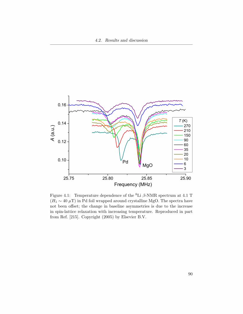
4.2. Results and discussion
Figure 4.1: Temperature dependence of the 8Li β-NMR spectrum at 4.1 T(H1 ∼ 40 µT) in Pd foil wrapped around crystalline MgO. The spectra havenot been offset; the change in baseline asymmetries is due to the increasein spin-lattice relaxation with increasing temperature. Reproduced in partfrom Ref. [215]. Copyright (2005) by Elsevier B.V.
90
4.2. Results and discussion
(νL = 25.836 MHz at 4.1 T). It is immediately apparent that the shift
of the Pd signal is quite large (compared to the simple metals), negative,
and T -dependent. The spectra are also quite broad and thus required a
relatively large H1 in order to obtain a signal of resonable amplitude. The
spectra shown in Fig. 4.1 are not offset; the decreasing off-resonance, baseline
asymmetry A0 as T is increased is consistent with the linear increase of T−11
with increasing T in metals (Chapter 1). Scanning a larger frequency range
at 270 K revealed no additional resonances, indicating that the spectrum is
not quadrupolar and that the stopping site(s) is(are) cubic.
The Pd spectra broaden considerably as the sample is cooled. As T is
lowered the line becomes more asymmetric, appearing as a main resonance
with a small amplitude, high frequency shoulder. This change in lineshape
may be due to multiple low-T stopping sites with similar resonance frequen-
cies. The Pd signal is described by two overlapping Gaussians (it will be
seen in the following Chapter that the use of two lines for the Pd signal
is indeed appropriate). The choice of Gaussian instead of Lorentzian line-
shapes is empirical; however, regardless of the lineshape used, an additional
Lorentzian needed to be included to account for the small amplitude, broad
component centred between the Pd and MgO signals. A single Lorentzian
is used to describe the MgO signal. Examples of these fits are shown in Fig.
4.2(a).
Using Eq. (1.16) with the MgO resonance frequency as ν0, the raw K(T )
obtained for the two Pd lines are shown in Fig. 4.2(b). As a convention in
this thesis, the more negatively shifted line is denoted as 1. The K values for
both lines show a similar trend with T , spanning a range of ≈ 800 ppm. The
resonance frequencies scale with H0, as expected for Knight shifts, further
ruling out a quadrupolar origin of the splitting. For instance, at 270 K and
H0 = 2.2 T, fitting the Pd signal to a single lineshape yields K ≈ −994(14)
ppm, consistent with the values observed at 4.1 T. Although these two lines
are reminiscent of the tentatively assigned O and S resonances in the group
11 metals, there are differences in the case of Pd; this is discussed further
in the next Chapter.
It is possible that the proximal field from the foil is influencing the res-
91
4.2. Results and discussion
Figure 4.2: (a) Representative fits; the Pd signal is fit using using twooverlapping Gaussian lineshapes (solid lines), a single Lorentzian lineshapeis used to fit the MgO signal (dash-dot line), and an additional Lorentzianlineshape is added to account for the broad background (dotted line). (b)The resulting K as a function of T for the two Pd lines.
92
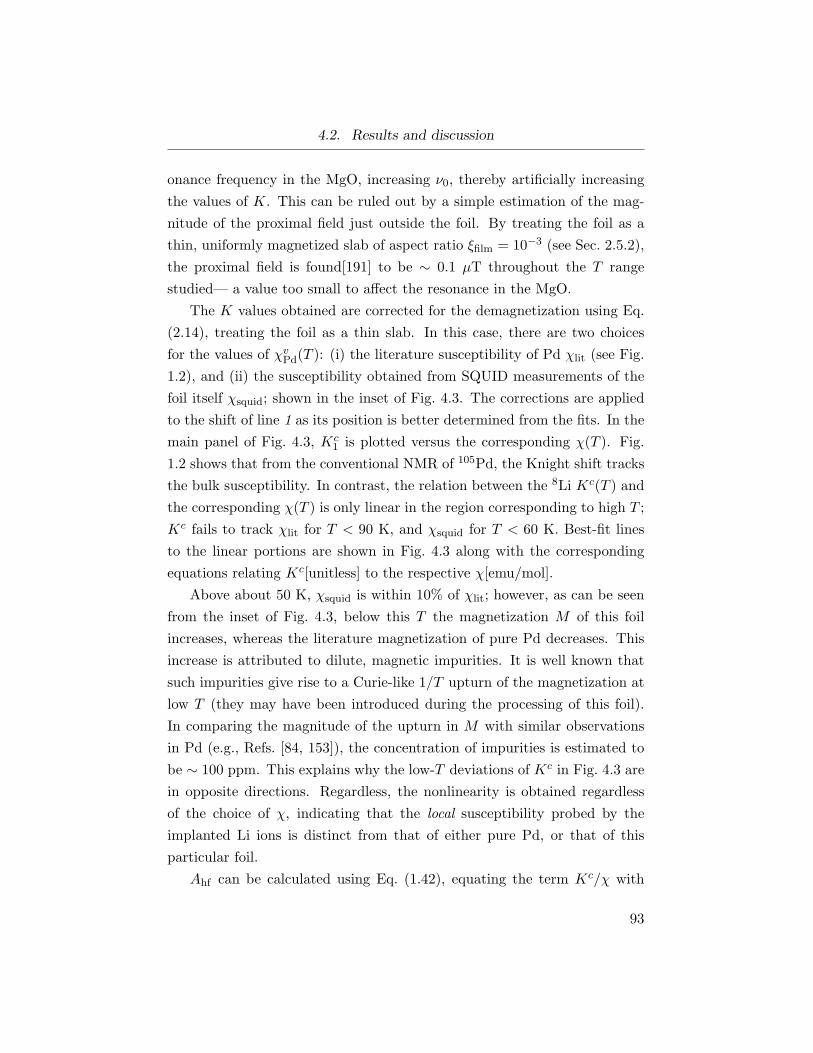
4.2. Results and discussion
onance frequency in the MgO, increasing ν0, thereby artificially increasing
the values of K. This can be ruled out by a simple estimation of the mag-
nitude of the proximal field just outside the foil. By treating the foil as a
thin, uniformly magnetized slab of aspect ratio ξfilm = 10−3 (see Sec. 2.5.2),
the proximal field is found[191] to be ∼ 0.1 µT throughout the T range
studied— a value too small to affect the resonance in the MgO.
The K values obtained are corrected for the demagnetization using Eq.
(2.14), treating the foil as a thin slab. In this case, there are two choices
for the values of χvPd(T ): (i) the literature susceptibility of Pd χlit (see Fig.
1.2), and (ii) the susceptibility obtained from SQUID measurements of the
foil itself χsquid; shown in the inset of Fig. 4.3. The corrections are applied
to the shift of line 1 as its position is better determined from the fits. In the
main panel of Fig. 4.3, Kc1 is plotted versus the corresponding χ(T ). Fig.
1.2 shows that from the conventional NMR of 105Pd, the Knight shift tracks
the bulk susceptibility. In contrast, the relation between the 8Li Kc(T ) and
the corresponding χ(T ) is only linear in the region corresponding to high T ;
Kc fails to track χlit for T < 90 K, and χsquid for T < 60 K. Best-fit lines
to the linear portions are shown in Fig. 4.3 along with the corresponding
equations relating Kc[unitless] to the respective χ[emu/mol].
Above about 50 K, χsquid is within 10% of χlit; however, as can be seen
from the inset of Fig. 4.3, below this T the magnetization M of this foil
increases, whereas the literature magnetization of pure Pd decreases. This
increase is attributed to dilute, magnetic impurities. It is well known that
such impurities give rise to a Curie-like 1/T upturn of the magnetization at
low T (they may have been introduced during the processing of this foil).
In comparing the magnitude of the upturn in M with similar observations
in Pd (e.g., Refs. [84, 153]), the concentration of impurities is estimated to
be ∼ 100 ppm. This explains why the low-T deviations of Kc in Fig. 4.3 are
in opposite directions. Regardless, the nonlinearity is obtained regardless
of the choice of χ, indicating that the local susceptibility probed by the
implanted Li ions is distinct from that of either pure Pd, or that of this
particular foil.
Ahf can be calculated using Eq. (1.42), equating the term Kc/χ with
93
4.2. Results and discussion
Figure 4.3: Demagnetization-corrected shifts Kc of line 1 versus χPd. Tem-perature is implicit, and decreases from left to right. The shifts were cor-rected for using, and subsequently plotted against, either the literature bulksusceptibility χlit, or the susceptibility of the same β-NMR foil sample χsquid.The latter was obtained from the magnetization measured in a SQUID at4.1 T (inset). In the high T region, Kc(T ) is linear with the respective χ(T )as shown by the best-fit lines.
94
4.2. Results and discussion
the slopes from the linear fits in Fig. 4.3, and assuming only octahedral
interstitial stopping sites (z = 6). The result is -1.28(5) kG/µB using χlit,
and -0.90(7) kG/µB using χsquid.
The linewidths and amplitudes of the Gaussians used to fit the Pd signals
are shown in Fig. 4.4. Focussing first on the widths [panel (a)], both lines
are relatively broad, and broaden further upon cooling. The sharp increase
in width occurs for both lines when T is less than about 50 K. This is the T
range where χsquid begins to deviate from χlit, likely due to dilute magnetic
impurities. These impurity moments are probably randomly distributed
throughout the foil, as are the final stopping sites of the Li ions. As a
consequence, when averaged over all distances, the impurity magnetization
gives rise to an inhomogeneous broadening, but does not affect the resonance
frequency, as mentioned in Sec. 1.2.1. Indeed, the increase in linewidth as
T → 0 is of the same order of magnitude as that calculated for dipolar
broadening following Ref. [37] by assuming 100 ppm of Fe impurities with
effective moments of 14µB[153]. Such an impurity concentration is consistent
with the quoted purity of this foil.
The corresponding amplitudes [panel (b)] decrease nearly linearly with
T . However, below 50 K where the Curie-like increase in the widths occurs,
there is scatter and the behaviour of the amplitudes is less obvious. This
is particularly the case for line 2, which shows a larger reduction in am-
plitude than that expected compared to its equality with line 1 above 50
K. For a constant H1, a broader line will have a smaller amplitude. The
significant broadening of such small signals increases the uncertainty in the
amplitudes, but inspection of Fig. 4.2(a) shows that at low T , the broad
component overlaps line 2. As temperature decreases, the widths increase
and amplitudes decrease, and it becomes less appropriate to treat the broad
component and line 2 separately. This likely leads to the peculiar behaviour
of the amplitude of line 2 and increasing the uncertainties in its K at low
T [Fig. 4.2(b)]. The inclusion of the broad component partly accounts for
the Pd lines not being described by pure Gaussians, and is attributed to the
magnetic impurities producing a pseudo-Lorentzian lineshape, i.e., increas-
ing the spectral weight in the “tails” of the Guassians[37]. Nonetheless, the
95
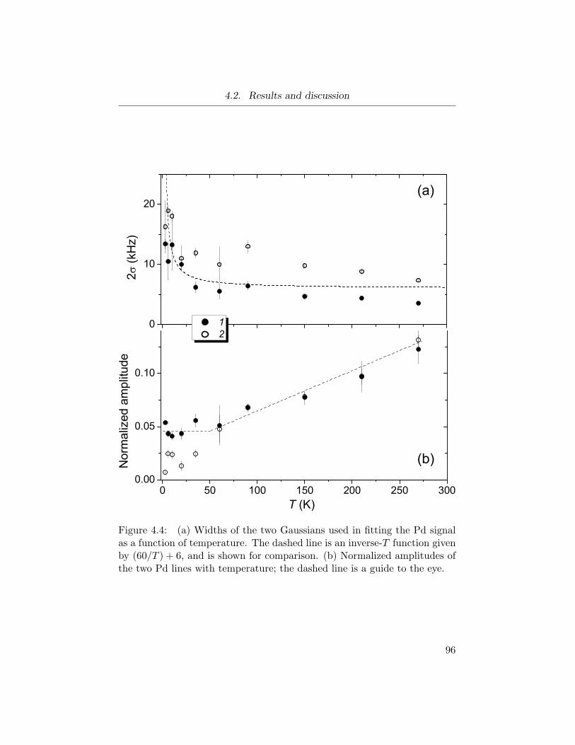
4.2. Results and discussion
Figure 4.4: (a) Widths of the two Gaussians used in fitting the Pd signalas a function of temperature. The dashed line is an inverse-T function givenby (60/T ) + 6, and is shown for comparison. (b) Normalized amplitudes ofthe two Pd lines with temperature; the dashed line is a guide to the eye.
96
4.3. Conclusions
present analysis is retained, particularly since the discussion of K is confined
to line 1, which has little overlap with the broad component. Moreover, in
light of the presence of dilute magnetic impurities, the present analysis is
quite satisfactory for an initial overview of the behaviour of 8Li in Pd.
Finally, the Korringa relation [Eq. (1.26)] can be applied to the above re-
sults. Using the ambient temperature relaxation rate measured previously[189]
(0.33 s−1), and taking K = 1 at 270 K, |Kc| is predicted to be ∼ 120
ppm, only about a quarter of what is observed. Similarly, for Kc = −428.5
ppm predicts a T1 ∼ 0.2 s, an order of magnitude faster than actually ob-
served. Combining this Kc with the relaxation rate gives K ∼ 13, about
1.5 times that measured for the host nuclei by conventional NMR[21] at 4
K (KPd = 9.4). Thus, even the smallest shift for 8Li in Pd is much larger
than expected from the Korringa relation; not surprising given that Pd is
far from being a simple metal.
4.3 Conclusions
In this short Chapter the general features of 8Li β-NMR in (bulk) Pd foil
were presented. In contrast to the shifts observed in noble metals or Al,
strongly T -dependent Knight shifts are observed in Pd, that are much larger
than the T−11 predicts. The resonance is relatively broad, and exhibits a
strong T -dependent width. At high temperature the shifts scale with sus-
ceptibility of pure Pd, but at low temperature this scaling no longer holds,
and is most likely a manifestation of the unique magnetic properties of this
host in response to the presence of the probe itself.
In order to verify that these intriguing results are truly intrinsic to 8Li+
in bulk Pd, the β-NMR of 8Li+ in a 100 nm film grown from a higher purity
Pd source was subsequently studied, and this is the topic of the following
Chapter.
97
Chapter 5
β-NMR of 8Li in a Bulk
Palladium Film
5.1 Introduction
In the previous Chapter, a brief study of the 8Li in a microns-thick Pd foil
sample revealed an unexpected low-temperature behaviour of the Knight
shift that is likely linked to the unique magnetic properties of Pd. In order
to verify that these results are indeed intrinsic to 8Li+ in bulk Pd, a 100
nm film of Pd was studied. By comparison to the findings in Au (Chapter
3), it is expected that a film of such thickness should give β-NMR results
similar to that of the 12.5 µm foil. Additionally, at low temperatures, the
magnetization of the foil indicated the presence of magnetic impurities that
broadened the linewidths of the resonances in that sample. This was avoided
for this film as it was grown from a higher purity source, and subsequently
protected by a Au capping layer.
Resonances are presented from this film, and the spin-lattice relaxation
rate is measured as a function of temperature in the foil. A combined anal-
ysis of the two data sets is presented in order to gain a more detailed un-
derstanding of the β-NMR of 8Li+ in bulk Pd. This is an important pre-
requisite to follow-up experiments to examine the possibility of studying
size-dependent magnetic properties of thin Pd films by β-NMR.
5.2 Results
The sample consists of a nominally 100 nm thick Pd film grown via e-beam
evaporation from a 99.99% source onto an epitaxially polished (100) STO
98
5.2. Results
substrate at 60–80 ◦C. The growth rate was ∼ 0.5 A/s under a background
pressure of ∼ 10−8 Torr. It was subsequently capped in situ with nomi-
nally 10 nm of Au. The thicknesses being established by a quartz crystal
growth-rate monitor. The Pd is found to be polycrystalline, but with a
(111) texture along the film normal as determined from X-ray diffraction
(thus less polycrystalline than the foil).
Resonances were recorded at an external field of 4.1 T for an implantation
energy of 11 keV and H1 ∼ 30 µT. For this ELi the TRIM.SP simulation of
the stopping profile indicates that no ions should stop in the STO substrate
[cf. Figs. B.2(b) and B.3]. Spectra were collected in the temperature range
of 8.5 K–270 K and are displayed in Fig. 5.1(a). The signals from Li in
the two layers could be assigned based on their relative amplitudes, and the
expected K in the respective metals (Chapters 3 and 4). The assignments
were confirmed by recording a spectrum for ELi = 0.9 keV for which the
signal assigned to ions in the Au is of larger amplitude compared to that
assigned to ions stopping in the Pd.
As expected from the measurements in the 12.5 µm foil presented in
the previous Chapter, the Pd signal is strongly T -dependent with a large,
negative K. The amplitude of the Pd signal also decreases with decreasing
T , as observed in the foil. As seen in the data of Chapter 3, the position
of the resonance from ions in the Au does not change with T , nor does its
amplitude. This is best seen in the normalized spectra in the inset of Fig.
5.1(b). It is noted that the Au signal is quite broad; however, this is not
discussed here, keeping the focus on exclusively the Pd resonances.
The Pd resonances from this film clearly appear as two partly resolved
lines throughout the entire T range studied. This a posteriori justifies the
use of two signals in fitting the resonances in the Pd foil in Chapter 4. As
discussed further below, in contrast to the foil spectra, there is no Curie-like
broadening of the resonances at low T , consistent with the higher purity
of this sample. The spectra were thus fit using two Lorentzian lineshapes
to account for the Pd signal, and a single Lorentzian lineshape for the Au
signal. This is illustrated for three representative spectra in Fig. 5.2. Close
inspection of these spectra shows that the choice of Lorentzians is motivated
99
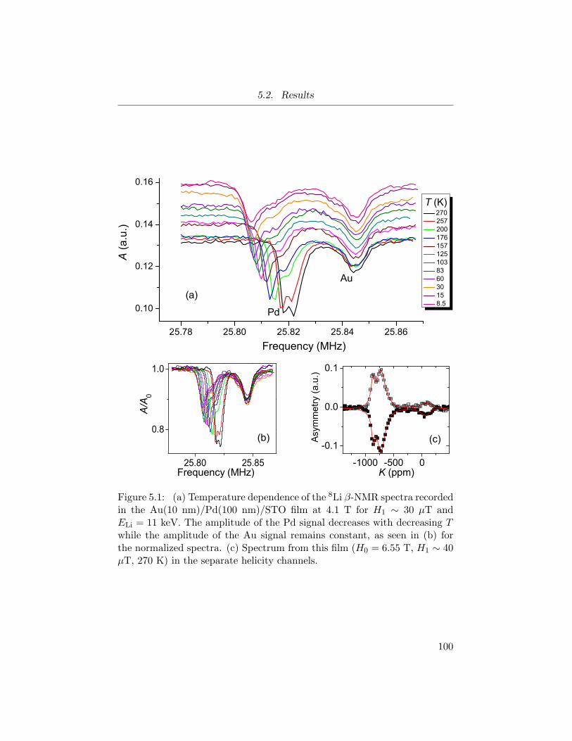
5.2. Results
Figure 5.1: (a) Temperature dependence of the 8Li β-NMR spectra recordedin the Au(10 nm)/Pd(100 nm)/STO film at 4.1 T for H1 ∼ 30 µT andELi = 11 keV. The amplitude of the Pd signal decreases with decreasing Twhile the amplitude of the Au signal remains constant, as seen in (b) forthe normalized spectra. (c) Spectrum from this film (H0 = 6.55 T, H1 ∼ 40µT, 270 K) in the separate helicity channels.
100
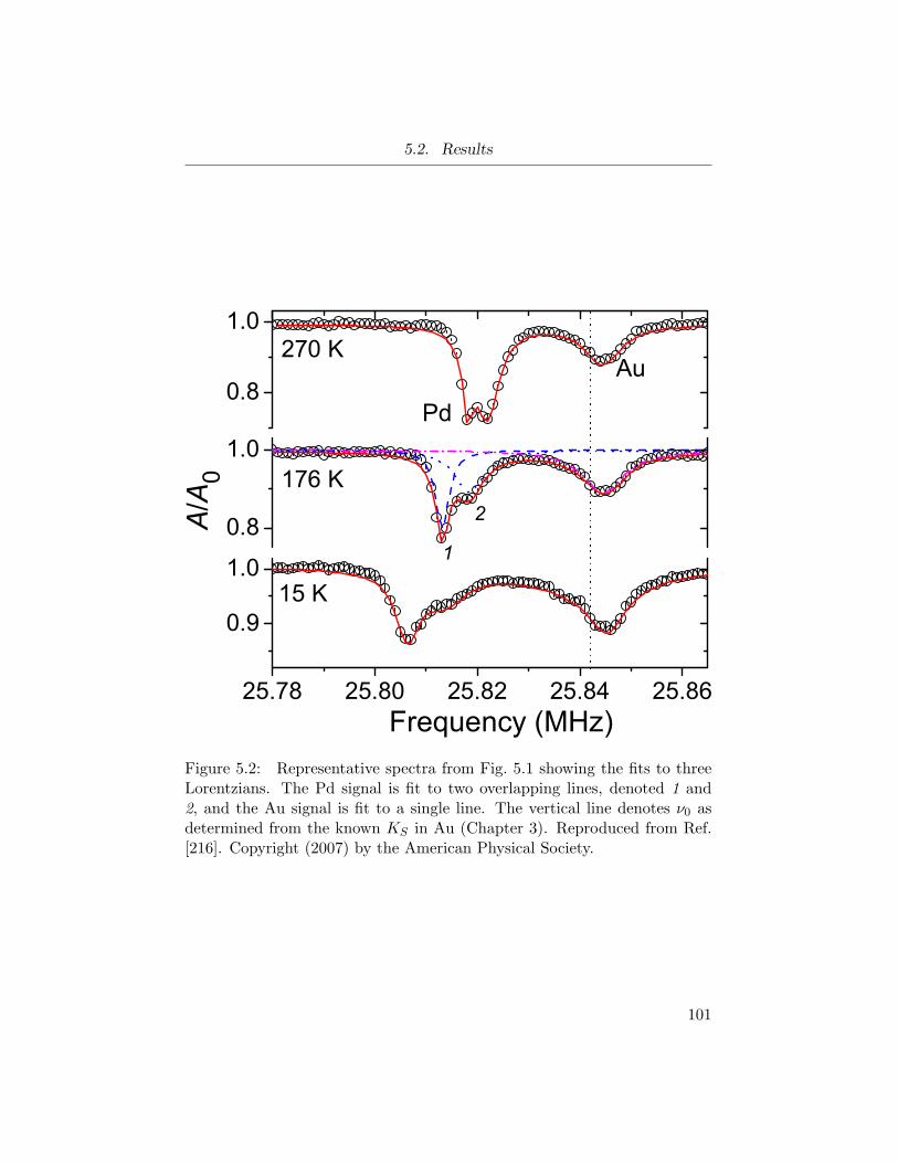
5.2. Results
Figure 5.2: Representative spectra from Fig. 5.1 showing the fits to threeLorentzians. The Pd signal is fit to two overlapping lines, denoted 1 and2, and the Au signal is fit to a single line. The vertical line denotes ν0 asdetermined from the known KS in Au (Chapter 3). Reproduced from Ref.[216]. Copyright (2007) by the American Physical Society.
101
5.2. Results
by the high rf power, but also to account for the small, high frequency tail
of the Pd signal. This is analogous to the high frequency broad component
observed in the foil spectra, but in the present resonances it is of reduced
amplitude and no additional lineshape was needed in the fits. It is noted
that in comparison, the low frequency end of the signal exhibits a sharper
cut-off. Random, dilute magnetic impurities are expected to produce sym-
metrically broadened resonances[37]. The asymmetric shape of these signals
instead suggests the shifts are distributed towards smaller values. As the
temperature is decreased, the frequency difference (i.e., splitting) between
the two lines comprising the resonances remains essentially constant.
Based on the results in Chap. 3, for T > 150 K, the Au signal would be
expected to appear as two resolved resonances attributed to ions stopping
in the S and O sites. However, as stated above, the resonance from the
Au is broad, and the two lines are not resolved. Additionally, near room
temperature the resonance from the Au is predominantly from ions assigned
to the S site. Using the established value of K for this site (+63 ppm) and
the frequency of the Au signal in this film at 270 K, a value of the reference
frequency ν0 was determined (vertical line in Fig. 5.2).
With the value of ν0 fixed, raw K values for the two Pd lines were
calculated using Eq. (1.16) and are shown in Fig. 5.3(a). The spectra show
no indication of a quadrupolar interaction in the individual helicities, e.g.,
Fig. 5.1(c). The K values of both Pd lines for H0 = 6.55 T at 270 K
[e.g., Fig. 5.1(c)] and 70 K are essentially equal to the shift values at 4.1
T, consistent with magnetic Knight shifts, as was concluded from the foil
resonances. The values of K for the two lines in the foil are also plotted in
panel (a) of Fig. 5.3. The similarity between the shifts from the two samples
is immediately evident; the magnitude of the shifts and their variation with
T are consistent between the two samples.
As the splitting between lines 1 and 2 in the film is small in comparison
to the shifts (∼ 200 ppm) and does not show any appreciable dependence
on T ; taking the average shift Kav simplifies the analysis, and this is plotted
Fig. 5.3(b). For the sake of comparison, Kav of the two lines from the foil
is also shown in Fig. 5.3(b). The magnitude and temperature dependence
102
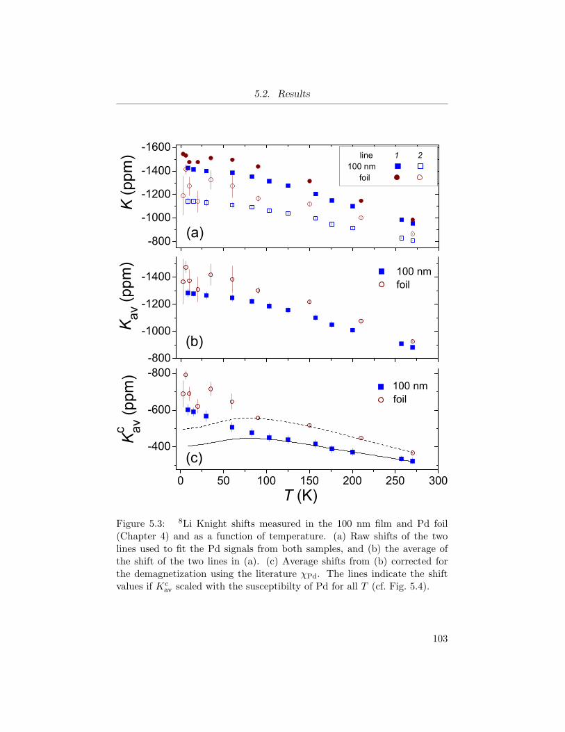
5.2. Results
Figure 5.3: 8Li Knight shifts measured in the 100 nm film and Pd foil(Chapter 4) and as a function of temperature. (a) Raw shifts of the twolines used to fit the Pd signals from both samples, and (b) the average ofthe shift of the two lines in (a). (c) Average shifts from (b) corrected forthe demagnetization using the literature χPd. The lines indicate the shiftvalues if Kc
av scaled with the susceptibilty of Pd for all T (cf. Fig. 5.4).
103
5.2. Results
of the two Kav(T ) are very similar as the values for the 100 nm are at most
about 10% smaller than those for the foil. This is most significant below 60
K where, due to the broadening attributed to dilute magnetic impurities,
the uncertainties and scatter in the shifts in the foil, especially of line 2,
are the largest. Overall, the agreement in the shifts from the two samples
can be considered quantitative. The small discrepancy is largely attributed
to systematics, particularly the broadening in the foil producing unresolved
lines, and the indirect determination of ν0 for the film data.
The Kav values are subsequently corrected for the effect of demagnetiza-
tion using Eq. (2.14). The choice of χ is clearly important here. In contrast
to a sample of foil, it is not feasible to measure the magnetization of this thin
film using SQUID magnetometry as the magnetization would be dominated
by the signal from the massive STO substrate. The susceptibility obtained
from the magnetization of the lower purity foil (inset of Fig. 4.3) is obviously
not appropriate. As the raw shifts are very similar in this film to those in
the bulk foil, the literature susceptibility of pure Pd χPd (Fig. 1.2) is used
in Eq. (2.14). The resulting corrected values are plotted in panel (c) of Fig.
5.3, where Kcav from the foil is also shown for comparison.
The corrected shifts from the film exhibit a monotonic increase toward
larger negative values upon cooling. At the lowest T Kcav has increased by a
factor ∼ 2 over the value near room T . The low temperature susceptibility
probed by the Li ions is not proportional to χPd, while at higher temper-
atures it scales linearly with χPd. This behaviour is seen in both the foil
and the film, and thus, is intrinsic to 8Li+ in Pd. Focussing on the film,
below about 110 K, Kcav increases roughly linearly with decreasing T . At
the lowest T , Kcav is about -200 ppm larger than if the scaling with χPd
were maintained, which is well outside the statistical errors. This low-T
deviation is not entirely surprising as χPd is very sensitive to the presence
of structural perturbations (like the 8Li probes), particularly for T in the
region of the susceptibility maximum and below. Thus, it seems reasonable
that for T < T ∗ ≃ 110 K a low temperature “defect” state is formed for8Li+ in Pd. In this T range, the local suceptibility sensed by the Li χloc
differs from that of χPd— it is notably enhanced over that of the pure host.
104
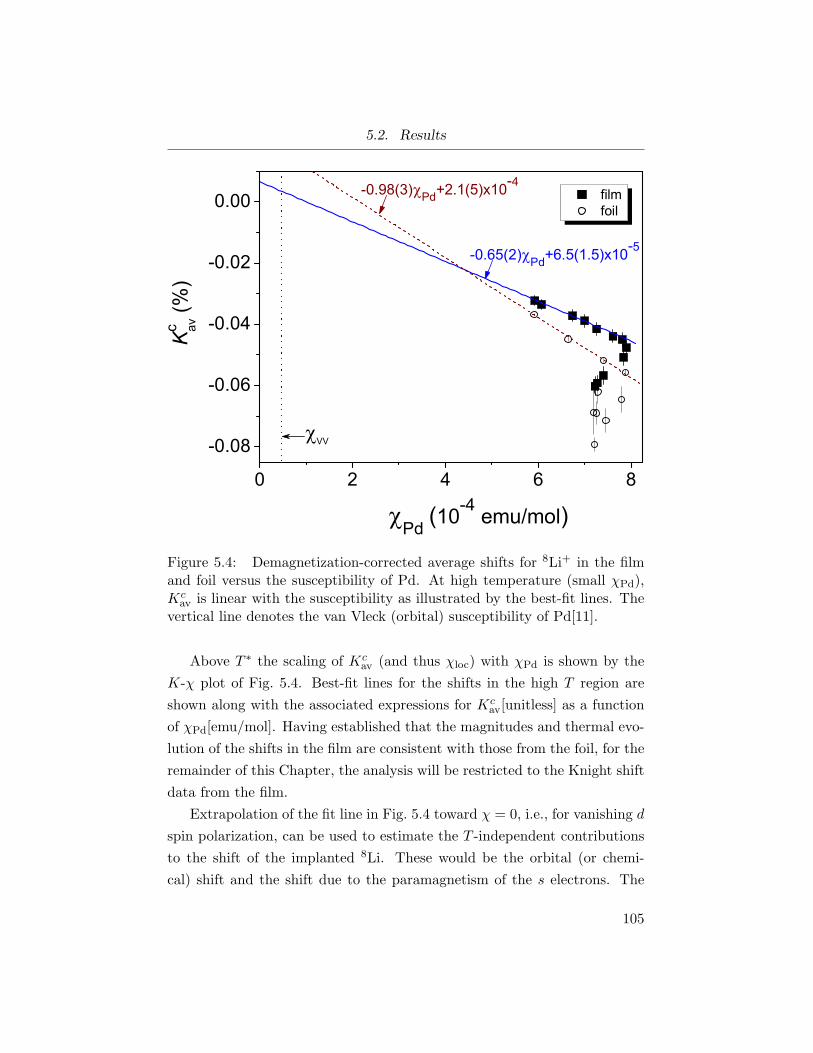
5.2. Results
Figure 5.4: Demagnetization-corrected average shifts for 8Li+ in the filmand foil versus the susceptibility of Pd. At high temperature (small χPd),Kc
av is linear with the susceptibility as illustrated by the best-fit lines. Thevertical line denotes the van Vleck (orbital) susceptibility of Pd[11].
Above T ∗ the scaling of Kcav (and thus χloc) with χPd is shown by the
K-χ plot of Fig. 5.4. Best-fit lines for the shifts in the high T region are
shown along with the associated expressions for Kcav[unitless] as a function
of χPd[emu/mol]. Having established that the magnitudes and thermal evo-
lution of the shifts in the film are consistent with those from the foil, for the
remainder of this Chapter, the analysis will be restricted to the Knight shift
data from the film.
Extrapolation of the fit line in Fig. 5.4 toward χ = 0, i.e., for vanishing d
spin polarization, can be used to estimate the T -independent contributions
to the shift of the implanted 8Li. These would be the orbital (or chemi-
cal) shift and the shift due to the paramagnetism of the s electrons. The
105
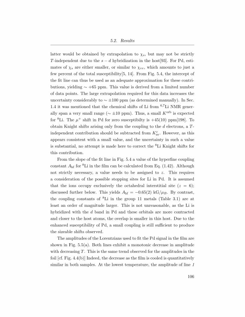
5.2. Results
latter would be obtained by extrapolation to χs, but may not be strictly
T -independent due to the s− d hybridization in the host[93]. For Pd, esti-
mates of χs are either smaller, or similar to χvv, which amounts to just a
few percent of the total susceptibility[5, 14]. From Fig. 5.4, the intercept of
the fit line can thus be used as an adequate approximation for these contri-
butions, yielding ∼ +65 ppm. This value is derived from a limited number
of data points. The large extrapolation required for this data increases the
uncertainty considerably to ∼ ±100 ppm (as determined manually). In Sec.
1.4 it was mentioned that the chemical shifts of Li from 6,7Li NMR gener-
ally span a very small range (∼ ±10 ppm). Thus, a small Korb is expected
for 8Li. The µ+ shift in Pd for zero susceptibilty is +45(10) ppm[198]. To
obtain Knight shifts arising only from the coupling to the d electrons, a T -
independent contribution should be subtracted from Kcav. However, as this
appears consistent with a small value, and the uncertainty in such a value
is substantial, no attempt is made here to correct the 8Li Knight shifts for
this contribution.
From the slope of the fit line in Fig. 5.4 a value of the hyperfine coupling
constant Ahf for 8Li in the film can be calculated from Eq. (1.42). Although
not strictly necessary, a value needs to be assigned to z. This requires
a consideration of the possible stopping sites for Li in Pd. It is assumed
that the ions occupy exclusively the octahedral interstitial site (z = 6);
discussed further below. This yields Ahf = −0.65(2) kG/µB. By contrast,
the coupling constants of 8Li in the group 11 metals (Table 3.1) are at
least an order of magnitude larger. This is not unreasonable, as the Li is
hybridized with the d band in Pd and these orbitals are more contracted
and closer to the host atoms, the overlap is smaller in this host. Due to the
enhanced susceptibility of Pd, a small coupling is still sufficient to produce
the sizeable shifts observed.
The amplitudes of the Lorentzians used to fit the Pd signal in the film are
shown in Fig. 5.5(a). Both lines exhibit a monotonic decrease in amplitude
with decreasing T . This is the same trend observed for the amplitudes in the
foil [cf. Fig. 4.4(b)] Indeed, the decrease as the film is cooled is quantitatively
similar in both samples. At the lowest temperature, the amplitude of line 1
106
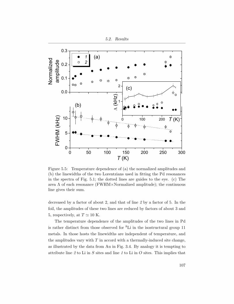
5.2. Results
Figure 5.5: Temperature dependence of (a) the normalized amplitudes and(b) the linewidths of the two Lorentzians used in fitting the Pd resonancesin the spectra of Fig. 5.1; the dotted lines are guides to the eye. (c) Thearea Λ of each resonance (FWHM×Normalized amplitude); the continuousline gives their sum.
decreased by a factor of about 2, and that of line 2 by a factor of 5. In the
foil, the amplitudes of these two lines are reduced by factors of about 3 and
5, respectively, at T ≃ 10 K.
The temperature dependence of the amplitudes of the two lines in Pd
is rather distinct from those observed for 8Li in the isostructural group 11
metals. In those hosts the linewidths are independent of temperature, and
the amplitudes vary with T in accord with a thermally-induced site change,
as illustrated by the data from Au in Fig. 3.4. By analogy it is tempting to
attribute line 2 to Li in S sites and line 1 to Li in O sites. This implies that
107
5.2. Results
the temperature range for which the Li site change occurs in Pd is higher
than room T . Thus, if the measurements could be extended to higher T it
would be expected that the amplitude of line 2 would continue to increase,
eventually saturating at some T , while the amplitude of line 1 would decrease
and eventually disappear completely. A difficulty with this scenario is the
small difference in K for lines 1 and 2. In the group 11 metals, K for the S
and O signals differs by a factor ∼ 2 (Table 3.1), while K for the two lines
of Pd differs by only a factor of ∼ 1.2. Moreover, for a site change which
occurs above room T , it is unlikely that the S sites would have appreciable
occupancy at the lowest temperatures and this line would not be expected
to be observed for all T . The S and O sites are sufficiently distinct that Li
occupying these sites should have clearly different shifts, as seen for Li in
the group 11 metals; however, the unique magnetic properties of Pd may
modify the shift of one or both sites such that the splitting between them
is reduced. Nonetheless, the Li is taken to be stopping in only the O sites
throughout the entire T range (see the Discussion). It is noted that absence
of the exact knowledge of the stopping site(s) does not preclude important
conclusions from being made.
The linewidths of the two Lorentzians are given in Fig. 5.5(b). They
are strongly temperature-dependent, exhibiting an increase upon cooling.
As found for the resonances from the foil [Fig. 4.4(a)], the width of line 2 is
always greater than that of line 1. However, unlike the foil, they do not show
the pronounced Curie-like impurity contribution at low T . This is consistent
with this film being of higher purity. The linewidths in this film are also
essentially equivalent to the values in the foil (for T above 60 K): ∼ 3 − 5
kHz and ∼ 7 − 12 kHz for lines 1 and 2, respectively. Put differently, the
widths of both lines double upon cooling from room temperature to 8 K. In
panel (c) of Fig. 5.5, the area of the two lines as a function of temperature is
shown. Below 250 K, they are essentially equal and approximately constant
with T . Thus, the decrease in amplitude is proportional to the increase
in width, and the number of spins contributing to each site is essentially
constant; this is further evidence against a thermally-induced site change.
In Fig. 5.6 the linewidths are re-plotted against T on a logarithmic scale
108
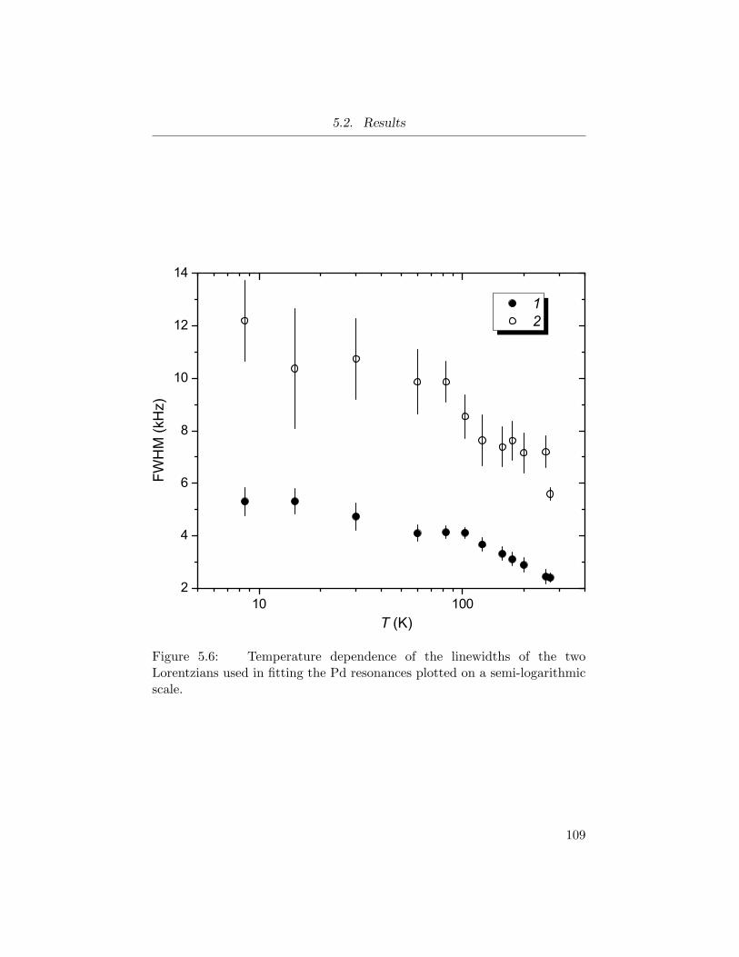
5.2. Results
Figure 5.6: Temperature dependence of the linewidths of the twoLorentzians used in fitting the Pd resonances plotted on a semi-logarithmicscale.
109
5.2. Results
providing a different perspective on their thermal variation. Such a pro-
nounced T -dependence indicates a contribution from a mechanism other
than static dipolar broadening from the host nuclei which is T -independent.
The powder-average, intrinsic (van Vleck) linewidths for undistorted O and
S sites in Pd are calculated to be 0.097 kHz and 0.051 kHz, respectively
[Eq. (1.43)]. These are essentially equal to those in Au. The only isotope of
Pd with a nuclear spin (105Pd) has a gyromagnetic ratio ∼ 4 times that of197Au, but has only a 22.3% natural abundance. The differences basically
cancel, so in the simplest estimate, the linewidths due to the static dipolar
broadening in Pd and Au are roughly the same. The linewidths observed
in Pd are thus indicative of a broadening due to inhomogeneities in the T -
dependent local magnetic field at the 8Li probes. Indeed, for larger H0 (6.55
T), the linewidths are broader, but based on the limited data, they do not
broaden in proportion to the change in applied field.
Turning to the spin-lattice relaxation rates, measurements of T−11 were
not performed in this film in order to avoid contamination from ions stopping
in the Au capping layer. Instead, the data were collected in a piece of the
same foil discussed in the previous Chapter. The data was collected for
H0 = 4.1 T, ELi = 28 keV, using a beam pulse of width δ = 4 s.
Representative time spectra spanning the T range studied are shown in
Fig. 5.7(a) along with the corresponding fits to Eqs. (2.7) and (2.8) as these
spectra were found to require two relaxing components to adequately decribe
the data. One component was constrained to be a small fraction (between
5 and 10%) of the total asymmetry, and have a relaxation rate an order of
magnitude faster than the majority component. A possible origin for this
small component is the fraction of ions that are backscattered, a second
is surface contamination. Regardless, the fits demonstrate that these time
spectra are well described by a single majority component. Thus, in spite
of the resonance spectra being comprised of two partially resolved lines, all
implanted ions can be taken to relax at the same rate for a given T . This is
not unreasonable since the shifts of the two lines differ by only ∼ 20%, and
so any small difference in the relaxation rates is not likely to be resolved in
the data.
110
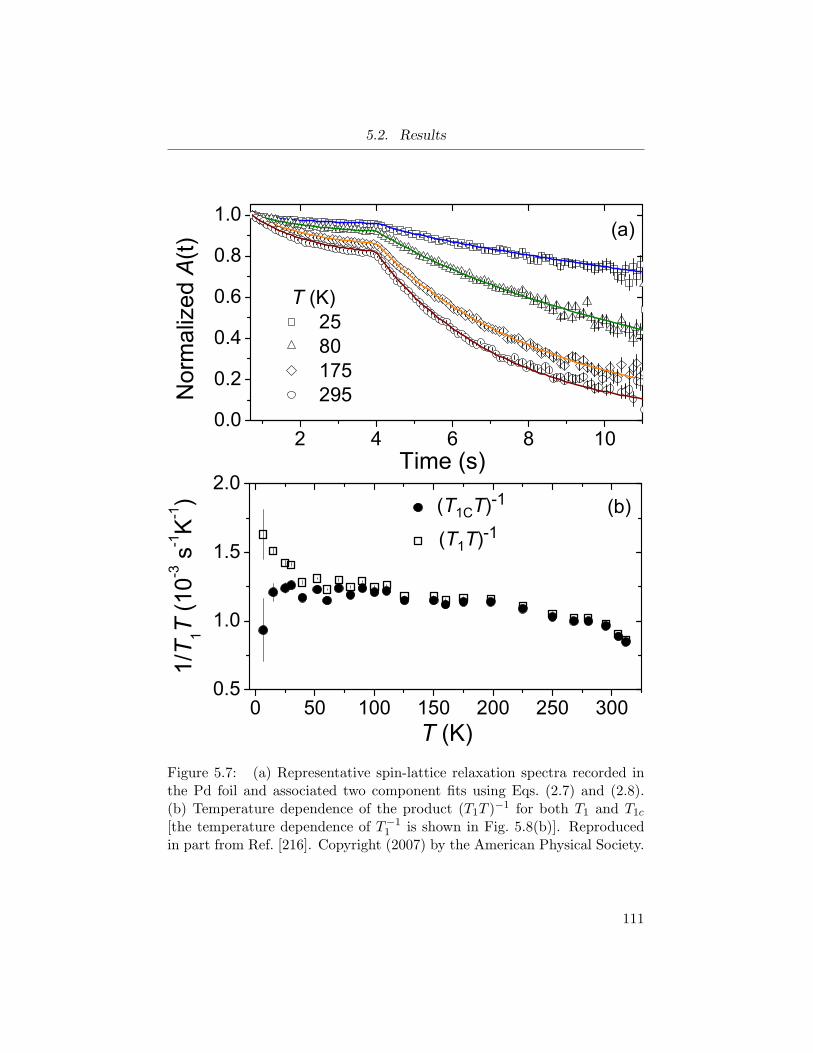
5.2. Results
Figure 5.7: (a) Representative spin-lattice relaxation spectra recorded inthe Pd foil and associated two component fits using Eqs. (2.7) and (2.8).(b) Temperature dependence of the product (T1T )−1 for both T1 and T1c
[the temperature dependence of T−11 is shown in Fig. 5.8(b)]. Reproduced
in part from Ref. [216]. Copyright (2007) by the American Physical Society.
111
5.2. Results
The resulting rates for the majority fraction as a function of T are dis-
played in Fig. 5.8(b). The rates exhibit an overall increase with increasing
T . This is also reflected by the essentially constant nature of 1/T1T over
most of the T range in Fig. 5.7(b). At a temperature just above T ∗, T−11
becomes sub-linear. However, for T ≤ 110 K, a linear fit to the rates yields
T−11 = 1.22(2)×10−3 s−1K−1T +4.5(9)×10−3 s−1 [solid line in Fig. 5.8(b)].
Note the rate obtained at room T is in very good agreement with the one re-
ported previously for 8Li in Pd at ambient temperature by Koenig et al.[189].
In order to isolate only the temperature-dependent contribution to T−11 , the
small T -independent term below T ∗ is subtracted and the resulting rates
denoted by T−11c . Since the T−1
1 data were collected over a T range spanning
two orders of magnitude, the effect of this correction is most significant only
at the lowest T where it removes the increase seen in 1/T1T . This is readily
seen in the temperature dependence of 1/T1cT that is also plotted in Fig.
5.7(b).
Measurements of 105Pd T−11 show that the rate is linear below about
150 K; whereas, above this T it becomes non-linear and appears to saturate
near room T [32]. This was discussed in Sec. 1.3 as being consistent with spin
fluctuation theory which predicts a thermal increase in the SF amplitudes
until a saturation is reached at Tsf whereupon they behave as effective local
moments with some degree of short-range order. The 8Li rates exhibit a
saturation consistent with the accepted value of Tsf ∼ 250 K for Pd[32, 95].
Very good agreement between these β-NMR rates and T−11d reported from
105Pd NMR[32] is evidenced in Fig. 5.9. The non-linearity of T−11 at high T is
thus characteristic of the nearly ferromagnetic nature of this host; however,
for T above room temperature, the limited data suggest a further decrease
in T−11 . This may be an indication of the onset of a thermally-actived site
change of the 8Li. The site at higher temperature would be characterized
by a smaller |K|, and hence a smaller slope, analogous to the decrease in
the slope of T−11 seen in the simple metals[185, 186, 187]. This observation
lends support to the belief that below room temperature the Li stopping
site does not change.
Nuclear spin-lattice relaxation rates provide an important test of spin
112
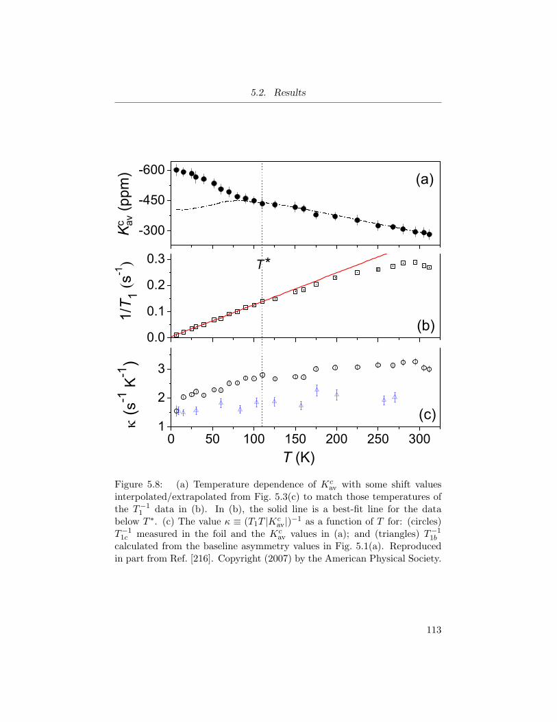
5.2. Results
Figure 5.8: (a) Temperature dependence of Kcav with some shift values
interpolated/extrapolated from Fig. 5.3(c) to match those temperatures ofthe T−1
1 data in (b). In (b), the solid line is a best-fit line for the databelow T ∗. (c) The value κ ≡ (T1T |Kc
av|)−1 as a function of T for: (circles)T−1
1c measured in the foil and the Kcav values in (a); and (triangles) T−1
1b
calculated from the baseline asymmetry values in Fig. 5.1(a). Reproducedin part from Ref. [216]. Copyright (2007) by the American Physical Society.
113
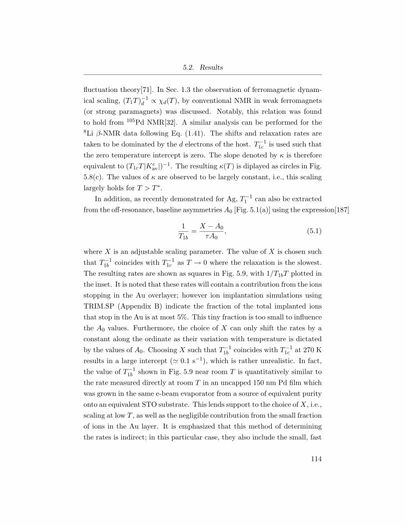
5.2. Results
fluctuation theory[71]. In Sec. 1.3 the observation of ferromagnetic dynam-
ical scaling, (T1T )−1d ∝ χd(T ), by conventional NMR in weak ferromagnets
(or strong paramagnets) was discussed. Notably, this relation was found
to hold from 105Pd NMR[32]. A similar analysis can be performed for the8Li β-NMR data following Eq. (1.41). The shifts and relaxation rates are
taken to be dominated by the d electrons of the host. T−11c is used such that
the zero temperature intercept is zero. The slope denoted by κ is therefore
equivalent to (T1cT |Kcav|)−1. The resulting κ(T ) is diplayed as circles in Fig.
5.8(c). The values of κ are observed to be largely constant, i.e., this scaling
largely holds for T > T ∗.
In addition, as recently demonstrated for Ag, T−11 can also be extracted
from the off-resonance, baseline asymmetriesA0 [Fig. 5.1(a)] using the expression[187]
1
T1b=X −A0
τA0, (5.1)
where X is an adjustable scaling parameter. The value of X is chosen such
that T−11b coincides with T−1
1c as T → 0 where the relaxation is the slowest.
The resulting rates are shown as squares in Fig. 5.9, with 1/T1bT plotted in
the inset. It is noted that these rates will contain a contribution from the ions
stopping in the Au overlayer; however ion implantation simulations using
TRIM.SP (Appendix B) indicate the fraction of the total implanted ions
that stop in the Au is at most 5%. This tiny fraction is too small to influence
the A0 values. Furthermore, the choice of X can only shift the rates by a
constant along the ordinate as their variation with temperature is dictated
by the values of A0. Choosing X such that T−11b coincides with T−1
1c at 270 K
results in a large intercept (≃ 0.1 s−1), which is rather unrealistic. In fact,
the value of T−11b shown in Fig. 5.9 near room T is quantitatively similar to
the rate measured directly at room T in an uncapped 150 nm Pd film which
was grown in the same e-beam evaporator from a source of equivalent purity
onto an equivalent STO substrate. This lends support to the choice ofX, i.e.,
scaling at low T , as well as the negligible contribution from the small fraction
of ions in the Au layer. It is emphasized that this method of determining
the rates is indirect; in this particular case, they also include the small, fast
114
5.2. Results
Figure 5.9: Comparison of the temperature dependence of (T1cT )−1 of 8Liin Pd foil (line, left ordinate) with the reported d electron contribution tothe relaxation rate from 105Pd NMR (circles; right ordinate)[32]. The ratesdetermined from the baseline asymmetry values T−1
1b from the resonancespectra in the film are also shown (squares; left ordinate). Inset: 1/T1bT(10−3 s−1 K−1) plotted over the same temperature range.
115
5.3. Discussion
component. Nonetheless, A0 values can in principle provide an alternative
way of obtaining T−11 [187], so it is interesting to compare these rates with
those determined directly. The rates obtained directly from the time spectra
in the foil are considered more reliable; however, the discrepancy between
the two sets provides motivation for further investigation. To this end, κ
calculated using T−11b and the corresponding Kc
av are also plotted as triangles
in Fig. 5.8(c). A close examination shows that for both sets of values κ begins
to decreases when the temperature is lowered below about 175 K.
5.3 Discussion
The observed resonances are comprised of two partially resolved lines that
exhibit similar thermal evolution of their shifts, widths and amplitudes.
Inspection of the resonances in the separate helicities does not indicate a
quadrupolar origin. By comparison with other fcc metals, one is lead to the
conclusion that the Li ions predominantly come to rest in the O sites over
the whole T range employed. This implies that there is a slight difference
in the hf interaction for a fraction of the ions although they all occupy the
same crystallographic lattice site.
This proposal is further substantiated by preliminary results from 8Li
β-NMR of a 100 nm (111)-oriented single crystal film of Pd grown epitaxi-
ally on an equivalent STO substrate[210]. The resonances from this sample
(not shown) exhibit identical relative shifts as a function of temperature,
but more importantly, they appear as a single, narrower line as opposed to
two overlapping ones. The resonance labelled 2 in the foil and the polycrys-
talline film discussed here is essentially absent in the single crystal spectra.
The major difference between polycrystalline and single crystal specimens
is the greater degree of orientation and lack of grain boundaries in the lat-
ter. Thus, it is suggested here that the two lines observed in polycrystalline
samples arise from ions are indeed in the same sites (O), but are distinct
as a consequence of the orientational heterogeneity. This implies the local
magnetic field probed by the 8Li depends on the orientation of the lattice
with respect to H0, albeit slightly. The two lines can then arise as a result of
116
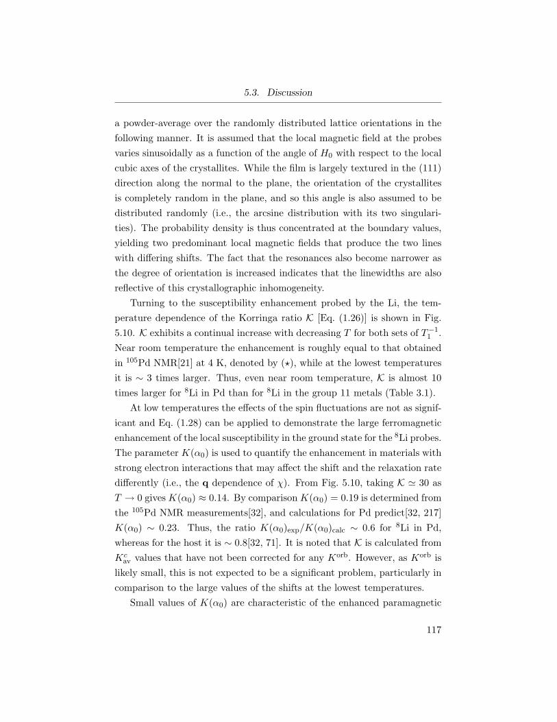
5.3. Discussion
a powder-average over the randomly distributed lattice orientations in the
following manner. It is assumed that the local magnetic field at the probes
varies sinusoidally as a function of the angle of H0 with respect to the local
cubic axes of the crystallites. While the film is largely textured in the (111)
direction along the normal to the plane, the orientation of the crystallites
is completely random in the plane, and so this angle is also assumed to be
distributed randomly (i.e., the arcsine distribution with its two singulari-
ties). The probability density is thus concentrated at the boundary values,
yielding two predominant local magnetic fields that produce the two lines
with differing shifts. The fact that the resonances also become narrower as
the degree of orientation is increased indicates that the linewidths are also
reflective of this crystallographic inhomogeneity.
Turning to the susceptibility enhancement probed by the Li, the tem-
perature dependence of the Korringa ratio K [Eq. (1.26)] is shown in Fig.
5.10. K exhibits a continual increase with decreasing T for both sets of T−11 .
Near room temperature the enhancement is roughly equal to that obtained
in 105Pd NMR[21] at 4 K, denoted by (⋆), while at the lowest temperatures
it is ∼ 3 times larger. Thus, even near room temperature, K is almost 10
times larger for 8Li in Pd than for 8Li in the group 11 metals (Table 3.1).
At low temperatures the effects of the spin fluctuations are not as signif-
icant and Eq. (1.28) can be applied to demonstrate the large ferromagnetic
enhancement of the local susceptibility in the ground state for the 8Li probes.
The parameter K(α0) is used to quantify the enhancement in materials with
strong electron interactions that may affect the shift and the relaxation rate
differently (i.e., the q dependence of χ). From Fig. 5.10, taking K ≃ 30 as
T → 0 gives K(α0) ≈ 0.14. By comparison K(α0) = 0.19 is determined from
the 105Pd NMR measurements[32], and calculations for Pd predict[32, 217]
K(α0) ∼ 0.23. Thus, the ratio K(α0)exp/K(α0)calc ∼ 0.6 for 8Li in Pd,
whereas for the host it is ∼ 0.8[32, 71]. It is noted that K is calculated from
Kcav values that have not been corrected for any Korb. However, as Korb is
likely small, this is not expected to be a significant problem, particularly in
comparison to the large values of the shifts at the lowest temperatures.
Small values of K(α0) are characteristic of the enhanced paramagnetic
117
5.3. Discussion
Figure 5.10: Temperature dependence of the Korringa ratio K calculatedfor Kc
av and T1c or T1b. The dashed line is a guide to the eye. (⋆) denotesthe value reported from 105Pd NMR at 4 K[21].
118
5.3. Discussion
state of nearly, or weakly, ferromagnetic metals, i.e., for enhancements of
the susceptibility that are confined to a small region around q ≃ 0. More-
over, they are an indication of the absence of any localized moments. By
contrast, for systems with localized impurity moments, K(α0) ∼ 1 and the
susceptibility is enhanced uniformly in q-space[71]. The 8Li data yield a
small K(α0) implying the susceptibility is enhanced in a small region of q-
space. The localized nature in q-space means the enhancement is extended
in real space.
The variation of K(α0) has been calculated for various values of α0[44,
45, 217]. Recall that α0 is a phenomenological measure of electron-electron
interactions, such that the Stoner enhancement factor can be approximated
as S ≈ (1 − α0)−1. The above K(α0) values for 8Li in Pd of ≈ 0.12 − 0.14
correspond to α0 ≈ 0.95 − 0.96, yielding S ∼ 20 − 25. Thus, the local
susceptibility probed by 8Li χloc is enhanced by a factor of at least 2 over
that of the pure host (as T → 0).
In Ref. [196], K of Li at O sites in Pd is reported from calculation to
be ∼ −700 ppm at 0 K. This agrees fairly well with the present low-T Kcav.
However, no details of the calculation were provided, so it is not known
what value of χPd was used to generate this shift and the agreement may
be fortuitous. It is reasonable that the deviation of the shifts from the host
susceptibility below T ∗ is related to the presence of the 8Li+ probe. No
observation of such an enhancement by any other implanted probe in this
metal has been reported to date.
In addition to the electronic modification of the host arising from the
hybridization of the Li 2s orbital with the d band, the local lattice relaxation
about the probe needs to be taken into consideration as a major factor in
determining χloc. Indeed, in keeping with the assumed assignment of the Li
probes to the O sites, a local expansion of the host lattice is thus expected as
discussed in Sec. 1.4. Importantly for Pd, a lattice expansion is predicted to
lead to a ferromagnetic ground state[135, 136, 137, 138, 139, 140]. Moreover,
Hjelm predicts that a lattice expansion will also significantly decrease the
critical field for a metamagnetic transition, concomitant with an increasing
orbital susceptibility with increasing applied field[133]. By comparison to
119
5.3. Discussion
the reported lattice expansions of octahedral interstitial H, B, and C in
Pd[218], Li can be estimated to produce an expansion ∼ 10%, sufficient to
substantially enhance the susceptibility.
Further, due to the anisotropy of the elastic constants of Pd, the magni-
tude of the expansion is expected to depend on crystallographic orientation[221].
However, the expansion must maintain the cubic symmetry of the stopping
site as there is no evidence for a quadrupole splitting due to an EFG at the Li
site. It is possible that the site is slightly non-cubic producing a small EFG
that gives rise to an unresolved, T -independent broadening of the resonances.
Regardless, this anisotropy is in keeping with the suggested origin of the two
resonance lines in polycrystalline specimens, although no anisotropy of the
resonances has been observed for 8Li in other cubic metals. The source of
this proposed anisotropic hf field must not depend strongly on temperature
as the splitting between the lines is approximately constant throughout the
temperature range. One possible origin is the spin-orbit interaction which,
due to the orbital motion of the electrons in the presence of a magnetic
field, can impart a preferred direction to the susceptibility[219, 220]. This
may further be related to the specific geometry of the crystallites. Slight
differences in the temperature dependence of the local lattice relaxation may
also contribute to the inhomogeneity of χloc that is evidenced through the
temperature dependence of the linewidths.
Furthermore, the volume dependence of the susceptibility of enhanced
magnetic metals is generally attributed to the volume dependence of the
Stoner parameter (i.e., of I)[222, 223, 224, 225] which is taken to be a local
atomic property, so this is consistent with the perturbation being confined
to a region of the Pd lattice in the immediate vicinity of the Li. Recall,
Zellermann et al. suggest that a small temperature dependence of I0 (∼ 1%)
is sufficient to account for the entire temperature dependence of χPd[109].
Thus, it is not unreasonable to consider a small enhancement of this param-
eter for, at least, the the Pd atoms nearest to the Li as a major contribution
to χloc.
A more intriguing characteristic of χloc is found by examination of the
temperature behaviour of the inverse of the shifts. In Fig. 5.11 |Kcav|−1
120
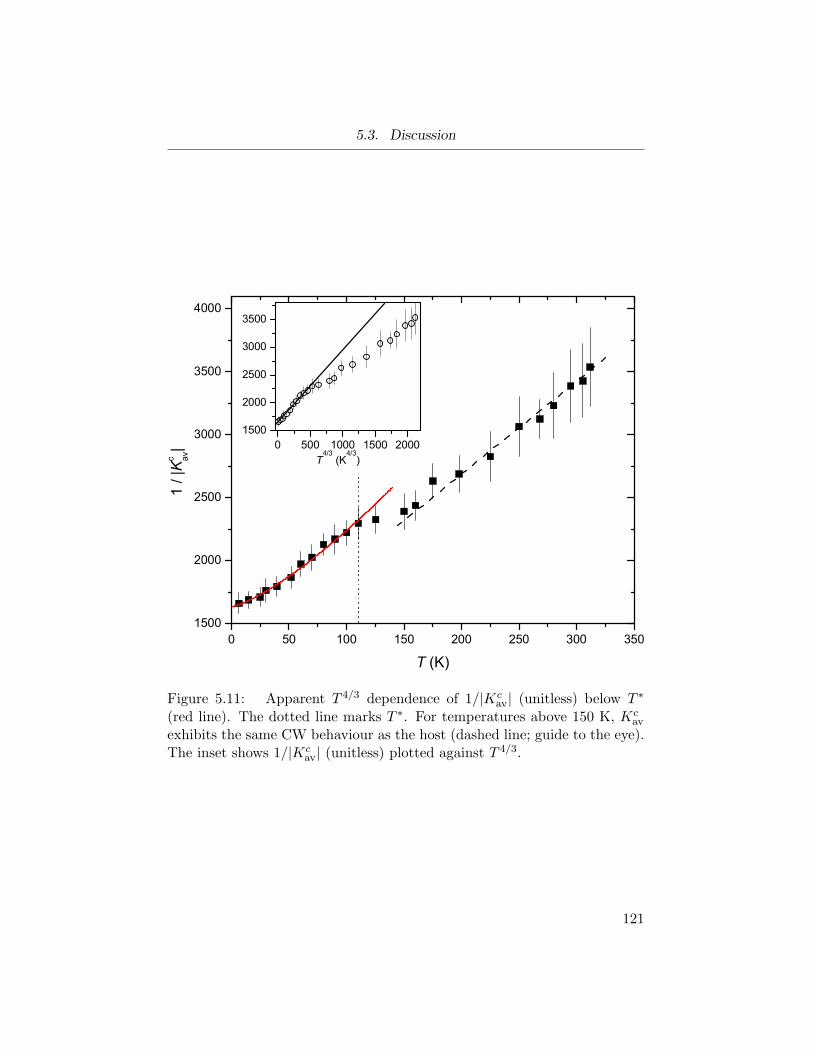
5.3. Discussion
Figure 5.11: Apparent T 4/3 dependence of 1/|Kcav| (unitless) below T ∗
(red line). The dotted line marks T ∗. For temperatures above 150 K, Kcav
exhibits the same CW behaviour as the host (dashed line; guide to the eye).The inset shows 1/|Kc
av| (unitless) plotted against T 4/3.
121
5.3. Discussion
(taken ∝ χ−1loc) is plotted as a function of T . For temperatures above
≈ 150 K, the inverse shifts are seen to follow the CW behaviour of the
host susceptibility[32]; however, for T < T ∗, they appear to be well de-
scribed by a behaviour ∝ T 4/3 as illustrated by the red line and in the inset.
This holds most strongly for temperatures below 50 K. Such a temperature
dependence is predicted from spin fluctuation theory for χ−1 of an itiner-
ant ferromagnet (in 3 dimensions) over a wide range of T just above the
transition temperature[54, 79, 87, 226]. This has also been experimentally
observed by magnetometry in several weak metallic ferromagnets where TC
was tuned via chemical doping[227, 228, 229]. For instance, the temper-
ature behaviour shown in Fig. 5.11 is identical with that reported in Ref.
[227] for Nb-doped ZrZn2 for a Nb concentration slightly above the criti-
cal concentration for which TC is suppressed to zero. The present results
strongly point to enhanced spin fluctuations in the region about the Li that
further enhance the propensity for ferromagnetic order, although there is no
evidence for static ordering.
The Li may be characterized as “nucleating” a region in its vicinity that
is even closer to ferromagnetic order than the enhanced paramagnetic host.
This is similar to “droplets” of local order in an otherwise non-ordered back-
ground that are theoretically predicted to be induced by defects in metals
that are proximal to magnetic groundstates[230]. The clear distinction here
is that there is no evidence of any longe-range ferromagnetic order induced
by the Li. The notion of a droplet of locally stronger enhancement may
indeed be a useful way to view the present results, in some ways analogous
to the concept of a magnetic polaron[231]. While the spin-lattice relaxation
rates show a linear increase with increasing T , consistent with the Korringa
mechansim, they are far slower than predicted from Kc using the Korringa
relation. This is surprising since a stronger local enhancement of the sus-
ceptibility would be predicted to give rise to stronger fluctuations thereby
increasing T−11 , particularly at lower temperatures. However, as pointed
out by Lederer[232] for the case of an isolated magnetic impurity in a nearly
ferromagnetic host, a local breakdown of the Korringa relation can be ex-
pected. This is due to the differing q dependence of K and T−11 . The shift
122
5.4. Conclusions
is sensitive to the static uniform susceptibility which, as discussed above,
is consistent with a large ferromagnetic enhancement in the region q ≃ 0.
Referring to Eq. (1.40), it is seen that T−11 depends on a sum over all q
components, and is less affected by the small region around q = 0 where the
uniform susceptibility is most enhanced. Thus, a stronger local enhancement
of the suceptibility need not correspond to faster relaxation rates. This is
equivalently manifest by the change in κ below T ∗.
5.4 Conclusions
In this Chapter a more detailed analysis of the behaviour of 8Li+ in a high-
purity, 100 nm Pd film was presented. The Knight shifts scale with χPd as
the temperature is lowered from room temperature down to T ∗ = 110 K.
This behaviour is similar to that observed in the foil indicating the behaviour
is intrinsic to 8Li in Pd. The resonances appear as two partially resolved
signals throughout the T range, but do not exhibit the thermal variation in
amplitudes (areas) of the resonances observed in other fcc metals. The two
lines are not assigned to 8Li stopping in distinct lattice sites, but are instead
taken to arise from ions in O sites that experience a subtly different hf fields
as a consequence of the lattice orientation. A powder-average of crystallite
orientations with respect to H0 is suggested to give rise to a local hf field
probability distribution that is concentrated at two values.
The linewidths are too broad to be solely from host nuclear dipoles, and
must be of magnetic origin. They are strongly dependent on temperature,
doubling as T is lowered from room temperature down to 8 K. However,
they do not show any sign of a Curie-like increase at the lowest temperatures
due to dilute magnetic impurities as in the case of the foil. The resonance
amplitudes decrease monotonically with decreasing T . This is simply a
consequence of the line broadening as the resonance areas remain essentially
constant.
Spin-lattice relaxation rates measurements in the foil, and extracted from
the resonance baseline asymmetries in the film, reveal an initial linear in-
crease with T at low temperatures, with an eventual saturation at higher
123
5.4. Conclusions
temperatures. The rates in the foil have a temperature dependence that is
identical to the d contribution to T−11 reported from conventional NMR of
the host. The data is observed to satisfy the relation predicted for ferro-
magnetic SFs of (T1T )−1 ∝ Kcav(T ) for T > T ∗.
Correspondingly, the local susceptibility probed by Li is enhanced over
that of the host below T ∗, and for T → 0 this corresponds to a Stoner
enhancement that is a factor of at least 2 greater than the pure host suscep-
tibility. The origin of this enhancement is not definite at present. However,
the importance of a local lattice expansion about the putative interstitial
ions, and an increase in the electron interaction parameter on the neighbour-
ing Pd atoms are pointed out in this regard. The inverse of the shifts for
T < T ∗ can be described by a T 4/3 variation which is expected for intinerant
ferromagnetic metals in a range of temperatures just above TC . This can
be viewed as the Li inducing a region locally that is closer to ferromagnetic
order— a droplet of “super-enhancement.” However, the spin-lattice relax-
ation rates do not exhibit a corresponding enhancement. This intriguing
observation requires further study, e.g., as a function of applied field, and
calls for ab initio calculations specifically treating the response of Pd to such
isolated defects.
124
Chapter 6
Summary and Future
Prospects
The results presented here describe the successful application of the β-NMR
technique to study the magnetism of transition metals. In particular, two
metals at the extremes of paramagnetism; namely, non-magnetic Au and
strongly exchange-enhanced, nearly ferromagnetic Pd. These results serve
as clear demonstrations of the power of this implanted probe technique for
studying materials typically not accessible by conventional NMR. Both met-
als were studied in the form of macroscopic foils, and also as thin films. The
latter samples illustrate the advantage of the TRIUMF low-energy β-NMR
facility using in-flight, optical polarization of the ions. Most other imple-
mentations of the β-NMR technique rely on polarized ions produced by
nuclear reactions which are subsequently implanted at MeV energies, thus
precluding their application to the study of thin film samples. This is a
testament to the immense potential of low-energy β-NMR for investigating
the magnetism of materials in reduced geometries, with the capability of
depth-resolved measurements when desired.
In a broader context, this work expands the knowledge of the hyperfine
interaction of implanted probes, as previous use of 8Li as a β-NMR probe
in either Au and Pd was scarce. First-principle calculations of the hyperfine
fields at impurities are stringent tests of theory. It is thus desirable to
test existing theories with as many probe-host combinations as possible.
Only in this way can potential deficiencies in present theories be identified
and improvements attempted, which may ultimately lead to new and more
accurate predictions. Calculations of the hf interaction of 8Li in the group 11
125
Chapter 6. Summary and Future Prospects
metals and Pd would certainly be desirable, not only in light of the present
results, but also in aiding the direction future studies.
Overall, the behaviour of 8Li in Au is very similar to that observed in the
other simple metals. Two distinct, narrow resonances are observed whose
frequencies do not show any dependence on temperature, in keeping with
the temperature-independent Pauli susceptibility. Only single resonances
are observed with no indication of quadrupole splitting, indicative of well-
defined, crystallographic stopping sites of cubic symmetry. Similar to the
case of the other three metals, these are taken to be the octahedral inter-
stitial and substitutional lattice sites. The resonance from ions in the latter
site appears only for temperatures greater than about 150 K, and is at-
tributed to a thermally-induced site change from the metastable interstitial
site. The linewidths are quite narrow and are not dependent on tempera-
ture (they broaden slightly in the T range of the site change). Such narrow
lines are also observed in Ag, but not in Al or polycrystalline Cu where
the two resonances are so broad they cannot be resolved. On the basis of
the present data, a comparison of the observed widths (in the limit of small
H1) with the calculated rigid-lattice dipolar widths is highly suggestive of a
local expansion about the interstitial ions and a local contraction about the
substitutional ions. No dependence on the mean implantation depth of the
probes was found for the resonances in Au.
The spin-lattice relaxation rate is independent of applied field for fields
greater than at least 15 mT. The rate at room temperature is less than half
as fast as that in the other three metals, and this is a notable distinction for
Au. Application of the Korringa relation for the substitutional ions yields a
ratio that is little enhanced over that predicted for a free-electron gas, i.e.,
K ≈ 1, and this is also the case for the other three metals. Except for Al
where they are equal, the 8Li enhancement values are slightly smaller than
those reported for the host nuclei by conventional NMR; the “disenhance-
ment” being greatest for Ag. Thus, the Li is not generating any significant
electronic correlations in its vicinity in these metals, signifying that it is
indeed probing their intrinsic electronic structure.
Preliminary T−11 data as a function of temperature in Au (not included
126
Chapter 6. Summary and Future Prospects
herein) are indicative of a rate that increases linearly with T , in keeping with
the Korringa mechanism of relaxation due to conduction electron spin-flip
scattering. The slope decreases in the T range of the site change. This is
analogous to what is observed in the other three simple metals. A study
of the intrinsic linewidths should be carried out as a function of larger H0
to be certain that the values are determined in the high-field limit where
the quadrupolar interaction for the host spins is not a complication. In this
regard, given that 197Au is 100% abundant (I = 32), it may be interesting to
attempt cross-relaxation measurements with 8Li in this host as well, which
have already been undertaken for 8Li in Cu[233].
The inertness of Au makes it prevalant as a protective capping layer
for many samples. Given its tendency to form flatter films[234] and its
higher density (i.e., greater stopping power), Au is an appealing candidate
for proximal magnetometry by 8Li β-NMR. Indeed, the induced magnetic
polarization of Au layers in contact with 3d ferromagnet layers is a topic
that has received little experimental attention[235]. The larger spin-orbit
coupling of Au can be expected to result in a magnetic coupling at the
interfaces that is distinct from that of other simple metals.
Turning to the results in Pd, the enhanced paramagnetism of this metal
makes β-NMR of this host more complicated, but simultaneously richer than
the simple metals. The results obtained are far from being fully understood,
and more work is needed; first-principle calculations would clearly be bene-
ficial in this regard.
The measured Knight shifts are negative for all temperatures studied,
and this is consistent with calculations of the hf field at 8Li in ferromagnetic
hosts like Ni as a consequence of the strong spin polarization from the d
electrons. The shifts track the temperature-dependent susceptibility of the
host for T > T ∗ ≈ 110 K, which is in keeping with the results of other
implanted probes like µ+ and 12B, as well as conventional NMR. However,
below this temperature the scaling breaks down; the local susceptibility
probed by the 8Li thus includes a contribution representing the response of
the host to the isolated defect and is no longer representative of the pure
host. Such a deviation from the host χ is hardly seen in the muon Knight
127
Chapter 6. Summary and Future Prospects
shifts in Pd. The previous 12B (and 12N) β-NMR measurements of Pd did
not extend below 100 K, so this appears to be a rare observation by NMR
of the temperature evolution of such a “defect” state in this metal. While
not a huge effect, the local susceptibility at the probe below T ∗ is greater
(∼ 30%) than that of the pure host and is consistent with the temperature
dependence expected for a weak ferromagnet in three dimensions just above
TC ; although, there is no evidence for static ordering.
The resonances appear as two partially resolved lines, but there is no
indication of a quadrupolar splitting. The amplitudes of the resonances
decrease with decreasing T due to line broadening. The resonances are
significantly broader than predicted for host spin dipolar broadening point-
ing to a likely magnetic origin. The behaviour is not in keeping with the
thermally-induced site changes observed in the isostructural simple metals.
Assignment of the lattice location(s) for the implanted ions is correspond-
ingly difficult; the analysis presented here assumes only the octahedral in-
terstitial site is occupied to any appreciable extent. The observation of two
resonances from the same stopping site leads to the suggestion that the hf
interaction is anisotropic; the pair of resonances arise due to an average over
the random distribution of crystallite orientations with respect to H0.
The spin-lattice relaxation rates measured in a foil sample initially in-
crease with increasing T , but become sub-linear above T ∗ tending to satu-
rate near room temperature. This is in keeping with the spin fluctuation-
dominated relaxation reported from 105Pd conventional NMR. Additionally,
below T ∗ where the shifts indicate a local enhancement of the static sus-
ceptibility, T−11 remains slower than expected. Above room T , T−1
1 further
decreases analogous to that observed in the T range of the the thermally-
induced site changes in the fcc simple metals. Higher temperature mea-
surements would be useful, but this requires a high temperature oven not
presently available. If the T−11 is instead calculated using the baseline asym-
metries from the resonances in a 100 nm film, a similar behaviour with T
is observed, but a stronger saturation occurs at a lower T (≃ 175 K) to a
rate that is roughly half as fast as that measured in the foil. Thus, a con-
sistent determination of both K and T−11 in the same film sample is a more
128
Chapter 6. Summary and Future Prospects
desirable situation.
Nonetheless, the shifts and relaxation rates could be analyzed analogous
to conventional NMR data to show that the prediction from spin fluctuation
theory of ferromagnetic dynamical scaling holds for 8Li β-NMR of Pd. This
demonstrates that β-NMR can be used to study the spin fluctuation (SF)
spectra of enhanced, or weakly, magnetic materials in a manner analogous
to conventional NMR. µSR can be used to probe the spin dynamics in such
systems[236], but the technique of β-NMR has not been applied for this
purpose. In this regard, the information obtained are complementary to that
from conventional NMR or inelatic neutron scattering, since light implanted
probes can access the interstitial regions and the presence of the probe itself
may affect the SFs locally. These additional perspectives on SFs can be
valuable in testing and refining theory, and thus further the understanding of
the role of these magnetic excitations of a given material and the occurance
of magnetism in general. For example, a possible initial candidate for this
type of study by β-NMR is the well-known, prototypical weak ferromagnet
Ni3Al. This system crystallizes in a structure that is analogous to the fcc
lattice of a pure metal, and recently susceptibility[228] and 27Al NMR[124]
were used to study the evolution of the SF spectrum following C intercalation
into the octahedral interstices.
Clearly further β-NMR of Pd is still in order. The onset of the intriguing
enhancement of the susceptibility is near 100 K, a relatively high temper-
ature in comparison to other “low temperature” phenomena. The Li may
be viewed as inducing a region of enhanced spin fluctuations that is locally
closer to ferromagnetic order than the pure host, described as a “droplet” of
super-enhancement. By all other reports, non-magnetic impurities cause a
reduction in the susceptibility of Pd. Thus, the origin of this effect certainly
deserves further investigation, and may also provide new insights into the
origin of the maximum observed in the susceptibility of the pure host.
Immediate future measurements should be extended to lower tempera-
tures, as well as carried out as a function of H0, particularly for lower values
than employed here. Systematic studies of the shifts, linewidths, and T−11
as a function of applied field may be useful in elucidating the origin of the
129
Chapter 6. Summary and Future Prospects
Li’s influence on the susceptibility. Also, the use of single crystal specimens
of different orientation, or alternatively, rotating a single crystal with re-
spect to H0, would be useful in addressing the proposed anisotropy of the
hf interaction.
Finally, some future extensions of β-NMR of Pd are mentioned. The
first involves the use of Pd layers in 8Li proximal magnetometry, or in stud-
ies of induced magnetic polarization. While more complicated than simple
metals like Ag or Au, magnetic polarization of Pd is far more facile. It is
also likely to yield a much more fascinating spatial response for which low-
energy β-NMR, with its depth resolution capability, is ideally equipped to
study. Indeed, it has been long known that Pd in contact with a ferromag-
netic substrate becomes polarized ferromagnetically, and that in many cases
this polarization extends a considerable distance from the interface[237, 238,
239, 240, 241, 242, 243]. It is quite conceivable that β-NMR could easily
address many aspects of these systems, like the temperature, applied field,
and distance dependence of this magnetic coupling. Rather analogous to
the magnetic proximity effect, is the proximity effect from a superconduc-
tor. There is considerable interest in understanding how the occurrence
of superconductivity is influenced at the interface between a superconduc-
tor and a ferromagnet, or equally an enhanced paramagnet[244]. A recent
example is such a study in Pd/Nb bilayers[245].
The second potential extension involves the study of Pd samples of re-
duced size. Owing to the strong dependence of the susceptibility on the
lattice structure, rather dramatic effects in the β-NMR of Pd can be ex-
pected for samples of thin films or supported nanocrystals[246]. In fact,
preliminary 8Li β-NMR results of thinner Pd films reveal a remarkable re-
duction in the Knight shift as a function of thickness[247]; cf. Fig. 2.5(b).
Further studies along this line would certainly be a valuable contribution
towards the understanding of magnetism at the nanoscale. In this regard,
the giant enhancement of the susceptibility observed for epitaxially strained
thin Pd in Au/Pd/Au sandwiches is recalled[139]. A multilayer comprised
of several repeating units of these sandwiches could easily be studied by low-
energy β-NMR, and the results would be of use in clarifying the influence
130
Chapter 6. Summary and Future Prospects
of lattice strain on the susceptibility.
131
Bibliography
[1] J. Kubler, Theory of Itinerant Electron Magnetism (Clarendon, Oxford,
2000).
[2] N.W. Ashcroft and N.D. Mermin, Solid State Physics (Holt-Saunders,
Philadelphia, 1976).
[3] C. Kittel, Introduction to Solid State Physics, 6th ed. (Wiley, New York,
1986).
[4] R.M. White, Quantum Theory of Magnetism, 2nd ed. (Springer-Verlag,
Berlin, 1983).
[5] J.J. van der Klink and H.B. Brom, Prog. Nucl. Magn. Reson. Spectrosc.
36, 89 (2000).
[6] P.K. Misra and L. Kleinman, Phys. Rev. B 5, 4581 (1972).
[7] M. Yasui, T. Takahashi, and J. Callaway, J. Phys.: Condens. Matter
3, 2679 (1991).
[8] The original reference for this is: R. Kubo and Y. Obata, J. Phys. Soc.
Jpn. 11, 547 (1956).
[9] R. Huguenin, G.P. Pells, and D.N. Baldock, J. Phys. F 1, 281 (1971).
[10] J. Benkowitsch and H. Winter, Z. Phys. B 50, 217 (1983).
[11] M. Deng, H. Freyer, J. Voitlander, and H. Ebert, J. Phys.: Condens.
Matter 13, 8551 (2001).
132
Bibliography
[12] V. Jaccarino, in Proceedings of the International School of Physics,
Enrico Fermi, Course XXXVII: Theory of Magnetism in Transition
Metals, edited by W. Marshall (Academic, New York, 1967), pp. 335–
385.
[13] A.J. Manuel and J.M.P. St. Quinton, Proc. R. Soc. London Ser. A 273,
412 (1963).
[14] J.A. Seitchik, A.C. Gossard, and V. Jaccarino, Phys. Rev. 136, A1119
(1964).
[15] H.C. Jamieson and F.D. Manchester, J. Phys. F 2, 323 (1972).
[16] F.H. Spedding and J.J. Croat, J. Chem. Phys. 58, 5514 (1973).
[17] R.J. Stierman, K.A. Gschneidner, Jr., T.-W.E. Tsang, F.A. Schmidt,
P. Klavins, R.N. Shelton, J. Queen, and S. Legvold, J. Magn. Magn.
Mater. 36, 249 (1983).
[18] N. Inoue and T. Sugawara, J. Phys. Soc. Jpn. 44, 440 (1978).
[19] J. Winter, Magnetic Resonance in Metals (Clarendon, Oxford, 1971).
[20] C.P. Slichter, Principles of Magnetic Resonance, 3rd. ed. (Springer-
Verlag, Berlin, 1990).
[21] G.C. Carter, L.H. Bennett, and D.J. Kahan, Metallic Shifts in NMR,
Progress in Materials Science Vol. 20, edited by B. Chalmers, J.W.
Christian, and T.B. Massalski (Pergamon Press, Oxford, 1977), Pt. 1.
[22] C.H. Townes, C. Herring, and W.D. Knight, Phys. Rev. 77, 852 (1950).
[23] W. Gotz and H. Winter, J. Phys.: Condens. Matter 5, 1707 (1993).
[24] A. Abragam and B. Bleaney, Electron Paramagnetic Resonance of
Transition Metal Ions (Clarendon, Oxford, 1970).
[25] G.D. Gaspari, W.-M. Shyu, and T.P. Das, Phys. Rev. 134, A852 (1964).
133
Bibliography
[26] A.M. Clogston, V. Jaccarino, and Y. Yafet, Phys. Rev. 134, A650
(1964).
[27] M. Shaham, U. El-Hanany, and D. Zamir, Phys. Rev. B 17, 3513 (1978).
[28] R. Krieger and J. Voitlander, Z. Phys. B 40, 39 (1980).
[29] H. Akai and T. Kotani, Hyperfine Interact. 120-121, 3 (1999).
[30] M. Battocletti and H. Ebert, Phys. Rev. B 64, 094417 (2001).
[31] K. Terakura, N. Hamada, T. Oguchi, and T. Asada, J. Phys. F 12,
1661 (1982).
[32] M. Takigawa and H. Yasuoka, J. Phys. Soc. Jpn. 51, 787 (1982).
[33] T. Asada, K. Terakura, and T. Jarlborg, J. Phys. F 11, 1847 (1981);
corrigendum: 14, 1989 (1984).
[34] J.B. Boyce and C.P. Slichter, Phys. Rev. Lett. 32, 61 (1974).
[35] J. Owen, M. Browne, W.D. Knight, and C. Kittel, Phys. Rev. 102,
1501 (1956).
[36] L.D. Graham and D.S. Schreiber, Phys. Rev. Lett. 17, 650 (1966).
[37] R.E. Walstedt and L.R. Walker, Phys. Rev. B 9, 4857 (1974).
[38] e.g., L.L. Lumata, K.Y. Choi, J.S. Brooks, A.P. Reyes, P.L. Kuhns, G.
Wu, and X.H. Chen, J. Phys.: Condens. Matter 22, 295601 (2010).
[39] T. Moriya, J. Phys. Soc. Jpn. 18, 516 (1963).
[40] W.W. Warren, Jr., G.F. Brennert, and U. El-Hanany, Phys. Rev. B 39,
4038 (1989).
[41] The original reference to this is: J. Korringa, Physica 16, 601 (1950).
[42] Y. Yafet and V. Jaccarino, Phys. Rev. 133, A1630 (1964).
[43] Y. Obata, J. Phys. Soc. Jpn. 18, 1020 (1963).
134
Bibliography
[44] A. Narath and H.T. Weaver, Phys. Rev. 175, 373 (1968).
[45] R.W. Shaw, Jr. and W.W. Warren, Jr., Phys. Rev. B 3, 1562 (1971).
[46] B.S. Shastry and E. Abrahams, Phys. Rev. Lett. 72, 1933 (1994).
[47] H.-O. Lee and H.-Y. Choi, Phys. Rev. B 62, 15120 (2000).
[48] e.g., R.E. Walstedt and Y. Yafet, Solid State Commun. 15, 1855 (1974).
[49] F.E. Hoare and J.C. Matthews, Proc. R. Soc. London Ser. A 212, 137
(1952).
[50] E. Sasioglu, C. Friedrich, and S. Blugel, Phys. Rev. B 83, 121101(R)
(2011).
[51] V. Thakor, J.B. Staunton, J. Poulter, S. Ostanin, B. Ginatempo, and
E. Bruno, Phys. Rev. B 68, 134412 (2003).
[52] e.g., I.D. Hughes, M. Dane, A. Ernst, W. Hergert, M. Luders, J. Poulter,
J.B. Staunton, A. Svane, Z. Szotek, and W.M. Temmerman, Nature
446, 650 (2007).
[53] E.C. Stoner, Proc. R. Soc. London Ser. A 154, 656 (1936); 165, 372
(1938).
[54] G.G. Lonzarich, in Electron: A Centenary Volume, edited by M. Spring-
ford (Cambridge University Press, Cambridge, 1997), Chap. 6.
[55] P.A. Wolff, Phys. Rev. 120, 814 (1960); T. Izuyama, D.-J. Kim, and
R. Kubo, J. Phys. Soc. Jpn. 18, 1025 (1963).
[56] S. Doniach, Proc. Phys. Soc. London 91, 86 (1967).
[57] J. Wahle, N. Blumer, J. Schlipf, K. Held, and D. Vollhardt, Phys. Rev.
B 58, 12749 (1998).
[58] O.K. Andersen, Phys. Rev. B 2, 883 (1970).
135
Bibliography
[59] F.M. Mueller, A.J. Freeman, J.O. Dimmock, and A.M. Furdyna, Phys.
Rev. B 1, 4617 (1970).
[60] T.J. Watson-Yang, B.N. Harmon, and A.J. Freeman, J. Magn. Magn.
Mater. 2, 334 (1976).
[61] A. Shabaev and D.A. Papaconstantopoulos, Phys. Rev. B 79, 064107
(2009).
[62] S.G. Das, D.D. Koelling, and F.M. Mueller, Solid State Commun. 12,
89 (1973).
[63] J.F. Janak, Phys. Rev. B 16, 255 (1977).
[64] J.R. Schrieffer, J. Appl. Phys. 39, 642 (1968).
[65] E. Stenzel and H. Winter, J. Phys. F 16, 1789 (1986).
[66] J.B. Staunton, J. Poulter, B. Ginatempo, E. Bruno, and D.D. Johnson,
Phys. Rev. B 62, 1075 (2000).
[67] T. Jeong, A. Kyker, and W.E. Pickett, Phys. Rev. B 73, 115106 (2006).
[68] D.A. Tompsett, R.J. Needs, F.M. Grosche, and G.G. Lonzarich, Phys.
Rev. B 82, 155137 (2010).
[69] M. Shimizu, Rep. Prog. Phys. 44, 21 (1981).
[70] O. Gunnarsson, J. Phys. F 6, 587 (1976).
[71] T. Moriya, Spin Fluctations in Itinerant Electron Magnetism (Springer-
Verlag, Berlin, 1985).
[72] S. Doniach and S. Engelsberg, Phys. Rev. Lett. 17, 750 (1966).
[73] M.T. Beal-Monod, S.-K. Ma, and D.R. Fredkin, Phys. Rev. Lett. 20,
929 (1968).
[74] K.K. Murata and S. Doniach, Phys. Rev. Lett. 29, 285 (1972).
136
Bibliography
[75] T.V. Ramakrishnan, Phys. Rev. B 10, 4014 (1974).
[76] N.F. Berk and J.R. Schrieffer, Phys. Rev. Lett. 17, 433 (1966).
[77] T. Takezawa, H. Nagara, and N. Suzuki, Phys. Rev. B 71, 012515
(2005); S.K. Bose, J. Phys.: Condens. Matter 20, 045209 (2008).
[78] G.G. Lonzarich and L. Taillefer, J. Phys. C 18, 4339 (1985).
[79] R.P. Smith, J. Phys.: Condens. Matter 21, 095601 (2009).
[80] P. Larson, I.I. Mazin, and D.J. Singh, Phys. Rev. B 69, 064429 (2004).
[81] D. Belitz, T.R. Kirkpatrick, and T. Vojta, Rev. Mod. Phys. 77, 579
(2005).
[82] The derivation of this model is given in the Appendix of Ref. [78].
[83] N.R. Bernhoeft, S.M. Hayden, G.G. Lonzarich, D.McK. Paul, and E.J.
Lindley, Phys. Rev. Lett. 62, 657 (1989).
[84] R. Doubble, S.M. Hayden, P. Dai, H.A. Mook, J.R. Thompson, and
C.D. Frost, Phys. Rev. Lett. 105, 027207 (2010).
[85] H. Nakamura, K. Yoshimoto, M. Shiga, M. Nishi, and K. Kakurai, J.
Phys.: Condens. Matter 9, 4701 (1997).
[86] e.g., V. Yushankhai, P. Thalmeier, and T. Takimoto, Phys. Rev. B 77,
125126 (2008).
[87] A. Ishigaki and T. Moriya, J. Phys. Soc. Jpn. 67, 3924 (1998).
[88] e.g., A.V. Ruban, S. Khemlevskyi, P. Mohn, and B. Johansson, Phys.
Rev. B 75, 054402 (2007).
[89] H. Yamada, Phys. Rev. B 47, 11211 (1993).
[90] I.F. Foulkes and B.L. Gyorffy, Phys. Rev. B 15, 1395 (1977); D. Fay
and J. Appel, ibid. 16, 2325 (1977); T. Jarlborg, Physica C 385, 513
(2003).
137
Bibliography
[91] P. Monthoux, D. Pines, and G.G. Lonzarich, Nature 450, 1177 (2007).
[92] P. Mohn and K. Schwarz, J. Magn. Magn. Mater. 104-107, 685 (1992).
[93] A.A. Povzner, A.G. Volkov, and A.N. Filanovich, Sov. Phys. Solid State
52, 2012 (2010) [Fiz. Tverd. Tela 52, 1879 (2010)].
[94] A. Khellaf and J.J. Vuillemin, J. Phys.: Condens. Matter 4, 1757
(1992); J.T. Schriempf, A.I. Schindler, and D.L. Mills, Phys. Rev. 187,
959 (1969); A.B. Kaiser and S. Doniach, Int. J. Magn. 1, 11 (1970);
R. Jullien, M.T. Beal-Monod, and B. Coqblin, Phys. Rev. B 9, 1441
(1974); A.P. Murani, Phys. Rev. Lett. 33, 91 (1974).
[95] K. Ikeda, S.K. Dhar, M. Yoshizawa, and K.A. Gschneidner, Jr., J.
Magn. Magn. Mater. 100, 292 (1991).
[96] S. Misawa, Phys. Lett. A 32, 153 (1970); 32, 541 (1970).
[97] G. Barnea, J. Phys. F 7, 315 (1977).
[98] G.M. Carneiro and C.J. Pethick, Phys. Rev. B 16, 1933 (1977).
[99] D.R. Grempel, Phys. Rev. B 27, 4281 (1983).
[100] E. Pamyatnykh, A. Poltavets, and M. Shabalin, J. Phys.: Condens.
Matter 9, 715 (1997).
[101] D.L. Maslov and A.V. Chubukov, Phys. Rev. B 79, 075112 (2009).
[102] H. Yamada and K. Terao, J. Phys.: Condens. Matter 6, 10805 (1994).
[103] S. Rowley, R. Smith, M. Dean, L. Spalek, M. Sutherland, M. Saxena,
P. Alireza, C. Ko, C. Liu, E. Pugh, S. Sebastian, and G. Lonzarich,
Phys. Status Solidi B 247, 469 (2010).
[104] A. Aguayo, I.I. Mazin, and D.J. Singh, Phys. Rev. Lett. 92, 147201
(2004).
[105] J. Kubler, Phys. Rev. B 70, 064427 (2004).
138
Bibliography
[106] e.g., A. Fujita, K. Fukamichi, J.-T. Wang, and Y. Kawazoe, Phys.
Rev. B 68, 104431 (2003).
[107] S. Sakai, R. Arita, and H. Aoki, Phys. Rev. Lett. 99, 216402 (2007).
[108] J.E. van Dam and O.K. Andersen, Solid State Commun. 14, 645
(1974).
[109] B. Zellermann, A. Paintner, and J. Voitlander, J. Phys.: Condens.
Matter 16, 919 (2004).
[110] C.J. Schinkel, F.R. de Boer, and B. de Hon, J. Phys. F 3, 1463 (1973).
[111] K.L. Liu, A.H. MacDonald, J.M. Daams, S.H. Vosko, and D.D.
Koelling, J. Magn. Magn. Mater, 12, 43 (1979).
[112] S.N. Kaul, J. Phys.: Condens. Matter 11, 7597 (1999).
[113] Y. Takahashi, J. Phys.: Condens. Matter 13, 6323 (2001).
[114] A.Z. Solontsov and D. Wagner, Phys. Rev. B 51, 12410 (1995).
[115] A. Solontsov, Int. J. Mod. Phys. B 19, 3631 (2005).
[116] V.P. Antropov and A. Solontsov, J. Appl. Phys. 109, 07E116 (2011).
[117] S. Hirooka, J. Phys.: Condens. Matter 12, 5669 (2000).
[118] E. Miyai and F.J. Ohkawa, Phys. Rev. B 61, 1357 (2000).
[119] A. Ishigaki and T. Moriya, J. Phys. Soc. Jpn. 65, 3402 (1996).
[120] H. Alloul and L. Mihaly, Phys. Rev. Lett. 48, 1420 (1982).
[121] K. Yoshimura, M. Mekata, M. Takigawa, Y. Takahashi, and H. Ya-
suoka, Phys. Rev. B 37, 3593 (1988).
[122] K. Yoshimura, T. Imai, T. Kiyama, K.R. Thurber, A.W. Hunt, and
K. Kosuge, Phys. Rev. Lett. 83, 4397 (1999).
139
Bibliography
[123] M. Corti, F. Carbone, M. Filibian, Th. Jarlborg, A.A. Nugroho, and
P. Carretta, Phys. Rev. B 75, 115111 (2007).
[124] B. Chen, H. Ohta, C. Michioka, Y. Itoh, and K. Yoshimura, Phys.
Rev. B 81, 134416 (2010).
[125] M. Majumder, K. Ghoshray, A. Goshray, B. Bandyopadhyay, and M.
Ghosh, Phys. Rev. B 82, 054422 (2010)
[126] e.g., B. Nowak, O. Zoga l, A. Pietraszko, R.E. Baumbach, M.B. Maple,
and Z. Henkie, Phys. Rev. B 79, 214411 (2009); C. Bourbonnais, P.
Wzietek, F. Creuzet, D. Jerome, P. Batail, and K. Bechgaard, Phys.
Rev. Lett. 62, 1532 (1989).
[127] e.g., C.-S. Lue and J.H. Ross, Jr., Phys. Rev. B 60, 8533 (1999).
[128] F.M. Muller, R. Gersdorf, and L.W. Roeland, Phys. Lett. A 31, 424
(1970).
[129] G.R. Stewart and B.L. Brandt, Phys. Rev. B 28, 2266 (1983).
[130] W. Joss, L.N. Hall, G.W. Crabtree, and J.J. Vuillemin, Phys. Rev. B
30, 5637 (1984).
[131] L.W. Roeland, J.C. Wolfrat, D.K. Mak, and M. Springford, J. Phys.
F 12, L267 (1982).
[132] T. Jarlborg and A.J. Freeman, Phys. Rev. B 23, 3577 (1981).
[133] A. Hjelm, Int. J. Mod. Phys. B 7, 275 (1993).
[134] E. Huger and K. Osuch, Eur. Phys. J. B 44, 145 (2005).
[135] H. Chen, N.E. Brener, and J. Callaway, Phys. Rev. B 40, 1443 (1989).
[136] V.L. Moruzzi and P.M. Marcus, Phys. Rev. B 39, 471 (1989).
[137] L. Fritsche, J. Noffke, and H. Eckardt, J. Phys. F 17, 943 (1987).
[138] S.C. Hong and J.I. Lee, J. Korean Phys. Soc. 52, 1099 (2008).
140
Bibliography
[139] M.B. Brodsky and A.J. Freeman, Phys. Rev. Lett. 45, 133 (1980).
[140] T. Jarlborg and A.J. Freeman, J. Appl. Phys. 53, 8041 (1982).
[141] Y. Kuk, L.C. Feldman, and P.J. Silverman, Phys. Rev. Lett. 50, 511
(1983).
[142] S.C. Hong, C.L. Fu, and A.J. Freeman, J. Appl. Phys. 63, 3655 (1988).
[143] cf. W. Gerhardt, F. Razavi, J.S. Schilling, D. Huser, and J.A. Mydosh,
Phys. Rev. B 24, 6744 (1981).
[144] D.J. Lam and K.M. Myles, J. Phys. Soc. Jpn. 21, 1503 (1966).
[145] T. Asada and K. Terakura, J. Phys. Soc. Jpn. 47, 1495 (1979).
[146] O. Loebich, Jr. and Ch.J. Raub, J. Less-Common. Met. 55, 67 (1977).
[147] T. Auerswald, H. Claus, and O. Meyer, Phys. Rev. B 43, 14232 (1991).
[148] R. Doclo, S. Foner, and A. Narath, J. Appl. Phys. 40, 1206 (1969).
[149] W. Sanger and J. Voitlander, Z. Phys. B 44, 283 (1981).
[150] R.J. Miller, T.O. Brun, and C.B. Satterthwaite, Phys. Rev. B 18, 5054
(1978).
[151] M.Mahnig and L.E. Toth, Phys. Lett. A 32, 319 (1970); H. Husemann
and H. Brodowsky, Z. Naturforsch. A 23, 1693 (1968).
[152] J. Crangle and W.R. Scott, J. Appl. Phys. 36, 921 (1965); G.J.
Nieuwenhuys, Adv. Phys. 24, 515 (1975).
[153] T. Herrmannsdorfer, S. Rehmann, W. Wendler, and F. Pobell, J. Low
Temp. Phys. 104, 49 (1996).
[154] G.G. Low and T.M. Holden, Proc. Phys. Soc. London 89, 119 (1966);
B.H. Verbeek, G.J. Nieuwenhuys, J.A. Mydosh, C. van Dijk, and B.D.
Rainford, Phys. Rev. B 22, 5426 (1980).
141
Bibliography
[155] S. Polesya, S. Mankovsky, O. Sipr, W. Meindl, C. Strunk, and H.
Ebert, Phys. Rev. B 82, 214409 (2010).
[156] e.g., N. Kioussis and J.W. Garland, Phys. Rev. Lett. 67, 366 (1991).
[157] J.D. Jackson, Classical Electrodynamics, 3rd ed. (Wiley, New York,
1999).
[158] e.g., A. Zangwill, Physics at Surfaces (Cambridge University Press,
Cambridge, 1988).
[159] e.g., J. Lu, P.L. Kuhns, M.J.R. Hoch, W.G. Moulton, and A.P. Reyes,
Phys. Rev. B 72, 054401 (2005); R.I. Salikhov, I.A. Garifullin, N.N.
Garif’yanov, L.R. Tagirov, K. Theis-Brohl, K. Westerholt, and H.
Zabel, Phys. Rev. Lett. 102, 087003 (2009).
[160] H.J. Jansch, P. Gerhard, and M. Koch, Proc. Nat. Acad. Sci. USA
101, 13715 (2004); A. Bifone, T. Pietrass, J. Kritzenberger, A. Pines,
and B.F. Chmelka, Phys. Rev. Lett. 74, 3277 (1995).
[161] E.B. Karlsson, Solid State Phenomena As Seen by Muons, Protons,
and Excited Nuclei (Clarendon, Oxford, 1995).
[162] A. Schenck, Muon Spin Rotation Spectroscopy: Principles and Appli-
cations in Solid State Physics (Adam Hilger, Bristol, 1985).
[163] R.F. Kiefl, G.D. Morris, P. Amaudruz, R. Baartman, J. Behr, J.H.
Brewer, J. Chakhalian, S. Daviel, J. Doornbos, S. Dunsiger, S.R. Kre-
itzman, T. Kuo, C.D.P. Levy, R. Miller, M. Olivo, R. Poutissou, G.W.
Wight, and A. Zelenski, Physica B 289-290, 640 (2000).
[164] e.g., E. Morenzoni, T. Prokscha, A. Suter, H. Luetkens, and R.
Khasanov, J. Phys.: Condens. Matter 16, S4583 (2004).
[165] Z. Salman, E.P. Reynard, W.A. MacFarlane, K.H. Chow, J.
Chakhalian, S. Kreitzman, S. Daviel, C.D.P. Levy, R. Poutissou, and
R.F. Kiefl, Phys. Rev. B 70, 104404 (2004).
142
Bibliography
[166] R.C. Haskell and L. Madansky, Phys. Rev. C 7, 1277 (1973).
[167] D. Borremans, D.L. Balabanski, K. Blaum,, W. Geithner, S. Gheysen,
P. Himpe, M. Kowalska, J. Lassen, P. Lievens, S. Mallion, R. Neugart,
G. Neyens, N. Vermeulen, and D. Yordanov, Phys. Rev. C 72, 044309
(2005).
[168] C.D. Gelatt, Jr., A.R. Williams, and V.L. Moruzzi, Phys. Rev. B 27,
2005 (1983).
[169] e.g., R. Bohmer, K.R. Jeffrey, and M. Vogel, Prog. Nucl. Magn. Reson.
Spectrosc. 50, 87 (2007).
[170] H. Akai, M. Akai, S. Blugel, B. Drittler, H. Ebert, K. Terakura, R.
Zeller, and P.H. Dederichs, Prog. Theor. Phys. Suppl. 101, 11 (1990).
[171] H. Fukuda and H. Akai, J. Phys. Soc. Jpn. 70, 2019 (2001).
[172] Y. Nojiri, K. Ishiga, T. Onishi, M. Sasaki, F. Ohsumi, T. Kawa, M.
Mihara, M. Fukuda, K. Matsuta, and T. Minamisono, Hyperfine Inter-
act. 120-121, 415 (1999).
[173] R. Pirlot, M. Cyamukungu, L. Grenancs, J. Lehmann, R. Coussement,
G. S’heeren, and K. Tompa, Hyperfine Interact. 80, 989 (1993).
[174] S.J. Blundell and S.F.J. Cox, J. Phys.: Condens. Matter 13, 2163
(2001).
[175] The original reference is: J.H. van Vleck, Phys. Rev. 74, 1168 (1948).
[176] O. Hartmann, Phys. Rev. Lett. 39, 832 (1977).
[177] B. Ittermann, G. Welker, F. Kroll, F. Mai, K. Marbach, and D. Peters,
Phys. Rev. B 59, 2700 (1999).
[178] H.-J. Stockmann, E. Jager, G. Sulzer, B. Ittermann, H. Ackermann, E.
Diehl, R. Dippel, B. Fischer, H.-P. Frank, and W. Seelinger, Hyperfine
Interact. 49, 235 (1989).
143
Bibliography
[179] M. Fullgrabe, B. Ittermann, H.-J. Stockmann, F. Kroll, D. Peters, and
H. Ackermann, Phys. Rev. B 64, 224302 (2001).
[180] T.K. McNab and R.E. McDonald, Phys. Rev. B 13, 34 (1976).
[181] T. Minamisono, Y. Nojiri, and K. Matsuta, Phys. Lett. A 94, 312
(1983).
[182] E. Jager, B. Ittermann, H.-J. Stockmann, K. Burkmann, B. Fischer,
H.-P. Frank, G. Sulzer, H. Ackermann, and P. Heitjans, Phys. Lett. A
123, 39 (1987).
[183] E. Jager, K. Burkmann, B. Fischer, H.-P. Frank, B. Ittermann, G.
Sulzer, H.-J. Stockmann, and H. Ackermann, Z. Phys. B 86, 389 (1992).
[184] G.D. Morris, W.A. MacFarlane, K.H. Chow, Z. Salman, D.J. Ar-
seneau, S. Daviel, A. Hatakeyama, S.R. Kreitzman, C.D.P. Levy, R.
Poutissou, R.H. Heffner, J.E. Elenewski, L.H. Greene, and R.F. Kiefl,
Phys. Rev. Lett. 93, 157601 (2004).
[185] Z. Salman, A.I. Mansour, K.H. Chow, M. Beaudoin, I. Fan, J. Jung,
T.A. Keeler, R.F. Kiefl, C.D.P. Levy, R.C. Ma, G.D. Morris, T.J.
Parolin, D. Wang, and W.A. MacFarlane, Phys. Rev. B 75, 073405
(2007).
[186] D. Wang, Z. Salman, K.H. Chow, I. Fan, M.D. Hossain, T.A. Keeler,
R.F. Kiefl, C.D.P. Levy, A.I. Mansour, G.D. Morris, M.R. Pearson, T.J.
Parolin, H. Saadaoui, M. Smadella, Q. Song, and W.A. MacFarlane,
Physica B 404, 920 (2009).
[187] M.D. Hossain, H. Saadaoui, T.J. Parolin, Q. Song, D. Wang, M.
Smadella, K.H. Chow, M. Egilmez, I. Fan, R.F. Kiefl, S.R. Kreitz-
man, C.D.P. Levy, G.D. Morris, M.R. Pearson, Z. Salman, and W.A.
MacFarlane, Physica B 404, 914 (2009).
[188] P. Ehrhart and H. Schultz, in Atomic Defects in Metals, edited by H.
Ullmaier, Landolt-Borstein, New Series, Group III, Vol. 25 (Springer-
Verlag, Heidelberg, 1991), Chap. 2.
144
Bibliography
[189] I. Koenig, D. Fick, S. Kossionides, P. Egelhof, K.-H. Mobius, and E.
Steffens, Z. Phys. A 318, 135 (1984).
[190] T.A. Keeler, Z. Salman, K.H. Chow, B. Heinrich, M.D. Hossain, B.
Kardasz, R.F. Kiefl, S.R. Kreitzman, C.D.P. Levy, W.A. MacFarlane,
O. Mosendz, T.J. Parolin, M.R. Pearson, and D. Wang, Phys. Rev. B
77, 144429 (2008).
[191] M. Xu, M.D. Hossain, H. Saadaoui, T.J. Parolin, K.H. Chow, T.A.
Keeler, R.F. Kiefl, G.D. Morris, Z. Salman, D. Wang, Q. Song, and
W.A. MacFarlane, J. Magn. Reson. 191, 47 (2008).
[192] H. Saadaoui, W.A. MacFarlane, Z. Salman, G.D. Morris, Q. Song,
K.H. Chow, M.D. Hossain, C.D.P. Levy, A.I. Mansour, T.J. Parolin,
M.R. Pearson, M. Smadella, D. Wang, and R.F. Kiefl, Phys. Rev. B
80, 224503 (2009).
[193] e.g., S.C. Hong, J.I. Lee, and R. Wu, Phys. Rev. B 75, 172402 (2007).
[194] e.g., Y. Oba, T. Sato, and T. Shinohara, Phys. Rev. B 78, 224417
(2008).
[195] K. Tompa, R. Pirlot, L. Grenacs, and J. Lehmann, Phys. Status Solidi
B 153, 721 (1989).
[196] M. Mihara, K. Matsuta, S. Kumashiro, M. Fukuda, S. Kosakai, Y.
Umemoto, M. Yoshikawa, R. Matsumiya, D. Nishimura, J. Komurasaki,
D. Ishikawa, M. Ogura, H. Akai, and T. Minamisono, Hyperfine In-
teract. 178, 73 (2007); M. Mihara, S. Kumashiro, K. Matsuta, Y.
Nakashima, H. Fujiwara, Y.N. Zheng, M. Ogura, H. Akai, M. Fukuda,
and T. Minamisono, ibid. 158, 361 (2004).
[197] J. Imazato, Y.J. Uemura, N. Nishida, R.S. Hayano, K. Nagamine, and
T. Yamazaki, J. Phys. Soc. Jpn. 48, 1153 (1980).
[198] F.N. Gygax, A. Hintermann, W. Ruegg, A. Schenck, and W. Studer,
Solid State Commun. 38, 1245 (1981).
145
Bibliography
[199] J. Brossel, A. Kastler, and J. Winter, J. Phys. Radium 13, 668 (1952).
[200] W.B. Hawkins and R.H. Dicke, Phys. Rev. 91, 1008 (1953).
[201] C.D.P. Levy, A. Hatakeyama, Y. Hirayama, R.F. Kiefl, R. Baartman,
J.A. Behr, H. Izumi, D. Melconian, G.D. Morris, R. Nussbaumer, M.
Olivo, M. Pearson, R. Poutissou, and G.W. Wight, Nucl. Instrum.
Methods B 204, 689 (2003).
[202] W. Widdra, M. Detje, H.-D. Ebinger, H.J. Jansch, W. Preyss, H. Re-
ich, R. Veith, D. Fick, M. Rockelein, and H.-G. Volk, Rev. Sci. Instrum.
66, 2465 (1995).
[203] Yu.G. Abov, A.D. Gulko, and F.S. Dzheparov, Sov. Phys. At. Nucl.
69, 1701 (2006) [Yad. Fiz. 69, 1737 (2006)].
[204] W.A. MacFarlane, G.D. Morris, K.H. Chow, R.A. Baartman, S.
Daviel, S.R. Dunsiger, A. Hatakeyama, S.R. Krietzman, C.D.P. Levy,
R.I. Miller, K.M. Nichol, R. Poutissou, E. Dumont, L.H. Greene, and
R.F. Kiefl, Physica B 326, 209 (2003).
[205] C.P. Poole, Jr. and H.A. Farach, Theory of Magnetic Resonance, 2nd
ed. (Wiley, New York, 1987).
[206] Z. Salman, R.F. Kiefl, K.H. Chow, M.D. Hossain, T.A. Keeler, S.R.
Kreitzman, C.D.P. Levy, R.I. Miller, T.J. Parolin, M.R. Pearson, H.
Saadaoui, J.D. Schultz, M. Smadella, D. Wang, and W.A. MacFarlane,
Phys. Rev. Lett. 96, 147601 (2006).
[207] S.R. Kreitzman, Hyperfine Interact. 65, 1055 (1990).
[208] S. Kazama and Y. Fukai, J. Less-Common Met. 53, 25 (1977).
[209] T.J. Parolin, J. Shi, Z. Salman, K.H. Chow, P. Dosanjh, H. Saadaoui,
Q. Song, M.D. Hossain, R.F. Kiefl, C.D.P. Levy, M.R. Pearson, and
W.A. MacFarlane, Phys. Rev. B 80, 174109 (2009).
[210] T. Wagner, G. Richter, and M. Ruhle, J. Appl. Phys. 89, 2606 (2001).
146
Bibliography
[211] W.A. MacFarlane, G.D. Morris, T.R. Beals, K.H. Chow, R.A. Baart-
man, S. Daviel, S.R. Dunsiger, A. Hatakeyama, S.R. Kreitzman, C.D.P.
Levy, R.I. Miller, K.M. Nichol, R. Poutissou, and R.F. Kiefl, Physica
B 326, 213 (2003).
[212] T.J. Parolin, Z. Salman, K.H. Chow, Q. Song, J. Valiani, H. Saadaoui,
A. O’Halloran, M.D. Hossain, T.A. Keeler, R.F. Kiefl, S.R. Kreitzman,
C.D.P. Levy, R.I. Miller, G.D. Morris, M.R. Pearson, M. Smadella, D.
Wang, M. Xu, and W.A. MacFarlane, Phys. Rev. B 77, 214107 (2008).
[213] e.g., A.F. McDowell, J. Magn. Reson. Ser. A 113, 242 (1995), and
references therein.
[214] F. Ohsumi, K. Matsuta, M. Mihara, T. Onishi, T. Miyake, M. Sasaki,
K. Sato, C. Ha, A. Morishita, T. Fujio, Y. Kobayashi, M. Fukuda, and
T. Minamisono, Hyperfine Interact. 120-121, 419 (1999).
[215] T.J. Parolin, Z. Salman, J. Chakhalian, D. Wang, T.A. Keeler, M.D.
Hossain, R.F. Kiefl, K.H. Chow, G.D. Morris, R.I. Miller, and W.A.
MacFarlane, Physica B 374-375, 419 (2006).
[216] T.J. Parolin, Z. Salman, J. Chakhalian, Q. Song, K.H. Chow, M.D.
Hossain, T.A. Keeler, R.F Kiefl, S.R. Kreitzman, C.D.P. Levy, R.I.
Miller, G.D. Morris, M.R. Pearson, H. Saadaoui, D. Wang, and W.A.
MacFarlane, Phys. Rev. Lett. 98, 047601 (2007).
[217] A. Narath and H.T. Weaver, Phys. Rev. B 3, 616 (1971).
[218] H.L.M. Bakker, M.J.C. de Jong, P.M. Oppeneer, R. Griessen, A. Lod-
der, R. Vis, and H. Brodowsky, J. Phys. F 16, 707 (1986).
[219] P.G. Averbuch and P.J. Segransan, Phys. Rev. B 4, 2067 (1971).
[220] E. Fawcett and V. Pluzhnikov, Physica 119B, 161 (1983).
[221] e.g., M. Doerr, S. Schonecker, A. Haase, E. Kampert, J.A.A.J. Paren-
boom, M. Richter, M. Rotter, M.S. Kim, and M. Loewenhaupt, J. Low
Temp. Phys. 159, 20 (2010).
147
Bibliography
[222] e.g., E. Fawcett, J.P. Maita, E. Bucher, and J.H. Wernick, Phys. Rev.
B 2, 3639 (1970).
[223] A.B. Kaiser and P. Fulde, Phys. Rev. B 37, 5357 (1988).
[224] A.B. Kaiser, A.M. Oles, and G. Stollhoff, Phys. Scr. 37, 935 (1988).
[225] A.S. Panfilov and I.V. Svechkarev, Int. J. Mod. Phys. B 7, 699 (1993).
[226] A.J. Millis, Phys. Rev. B 48, 7183 (1993).
[227] D.A. Sokolov, M.C. Aronson, W. Gannon, and Z. Fisk, Phys. Rev.
Lett. 96, 116404 (2006).
[228] B. Chen, C. Michioka, Y. Itoh, and K. Yoshimura, J. Phys. Soc. Jpn.
77, 103708 (2008).
[229] J. Yang, B. Chen, H. Ohta, C. Michioka, K. Yoshimura, H. Wang, and
M. Fang, Phys. Rev. B 83, 134433 (2011).
[230] A.J. Millis, D.K. Morr, and J. Schmalian, Phys. Rev. Lett. 87, 167202
(2001).
[231] e.g., P.-G. de Gennes, Phys. Rev. 118, 141 (1960); V.G. Storchak,
J.H. Brewer, R.L. Lichti, T.A. Lograsso, and D.L. Schlagel, Phys. Rev.
B 83, 140404(R) (2011).
[232] P. Lederer, Solid State Commun. 7, 209 (1969).
[233] A.I. Mansour, G.D. Morris, Z. Salman, K.H. Chow, T. Dunlop, J.
Jung, I. Fan, W.A. MacFarlane, R.F. Kiefl, T.J. Parolin, H. Saadaoui,
D. Wang, M.D. Hossain, Q. Song, M. Smadella, O. Mosendz, B. Kar-
dasz, and B. Heinrich, Physica B 401-402, 662 (2007).
[234] e.g., A.J. Francis and P.A. Salvador, J. Mater. Res. 22, 89 (2007).
[235] F. Wilhelm, M. Angelakeris, N. Jaouen, P. Poulopoulos, E.Th. Pa-
paioannou, Ch. Mueller, P. Fumagalli, A. Rogalev, and N.K. Flevaris,
Phys. Rev. B 69, 220404(R) (2004); T. Emoto, N. Hosoito, and T.
Shinjo, J. Magn. Magn. Mater. 189, 136 (1998).
148
Bibliography
[236] e.g., A. Yaouanc, P. Dalmas de Reotier, P.C.M. Gubbens, S. Sakarya,
G. Lapertot, A.D. Hillier, and P.J.C. King, J. Phys.: Condens. Matter
17, L129 (2005).
[237] U. Gradmann and R. Bergholz, Phys. Rev. Lett. 52, 771 (1984).
[238] J. Dorantes-Davila, H. Dreysse, and G.M. Pastor, Phys. Rev. Lett.
91, 197206 (2003); P.F. Carcia, A.D. Meinhaldt, and A. Suna, Appl.
Phys. Lett. 47, 178 (1985).
[239] E.E. Fullerton, D. Stoeffler, K. Ounadjela, B. Heinrich, Z. Celinski,
and J.A.C. Bland, Phys. Rev. B 51, 6364 (1995); Z. Celinski, B. Hein-
rich, J.F. Cochran, W.B. Muir, A.S. Arrott, and J. Kirschner, Phys.
Rev. Lett. 65, 1156 (1990).
[240] L. Cheng, Z. Altounian, D.H. Ryan, J.O. Strom-Olsen, M. Sutton,
and Z. Tun, Phys. Rev. B 69, 144403 (2004).
[241] H.H. Bertschat, H.-H. Blaschek, H. Granzer, K. Potzger, S. Seeger,
W.-D. Zeitz, H. Niehus, A. Burchard, D. Forkel-Wirth, and ISOLDE
Collaboration, Phys. Rev. Lett. 80, 2721 (1998).
[242] T. Manago, T. Ono, H. Miyajima, K. Kawaguchi, and M. Sohma, J.
Phys. Soc. Jpn. 68, 3677 (1999).
[243] Y.N. Kim, E.K. Lee, Y.B. Lee, H. Shim, N.H. Hur, and W.S. Kim, J.
Am. Chem. Soc. 126, 8672 (2004).
[244] e.g., D. Katayama, A. Sumiyama, and Y. Oda, Phys. Rev. B 68,
132502 (2003).
[245] A. Potenza, M.S. Gabureac, and C.H. Marrows, Phys. Rev. B 76,
014534 (2007); J. Appl. Phys. 103, 07C703 (2008).
[246] e.g., F. Silly and M.R. Castell, Phys. Rev. Lett. 94, 046103 (2005); F.
Silly, A.C. Powell, M.G. Martin, and M.R. Castell, Phys. Rev. B 72,
165403 (2005).
149
Bibliography
[247] T.J. Parolin, Z. Salman, J. Chakhalian, Q. Song, K.H. Chow, G.D.
Morris, M. Egilmez, I. Fan, M.D. Hossain, T.A. Keeler, R.F. Kiefl,
S.R. Kreitzman, C.D.P. levy, A.I. Mansour, R.I. Miller, M.R. Pearson,
H. Saadaoui, M. Smadella, D. Wang, M. Xu, and W.A. MacFarlane,
Physica B 404, 917 (2009).
[248] G. Friedlander, J.W. Kennedy, E.S. Macias, and J.M. Miller, Nuclear
and Radiochemistry, 3rd ed. (Wiley, New York, 1981).
[249] K. Heyde, Basic Ideas and Concepts in Nuclear Physics, 3rd ed. (In-
stitute of Physics, Bristol, 2004), Chap. 5.
[250] E. Segre, Nuclei and Particles, 2nd ed. (Benjamin/Cummings, Read-
ing, MA, 1977).
[251] H.J. Lipkin, Beta Decay for Pedestrians (Dover, Mineola, NY, 2004),
Chap. 2.
[252] S.G. Crane, S.J. Brice, A. Goldschmidt, R. Gukert, A. Hime, J.J.
Kitten, D.J. Vieira, and X. Zhao, Phys. Rev. Lett. 86, 2967 (2001).
[253] L.M. Chirovsky, W.P. Lee, A.M. Sabbas, J.L. Groves, and C.S. Wu,
Phys. Lett. B 94, 127 (1980).
[254] J. Sromicki, M. Allet, K. Bodek, W. Hajdas, J. Lang, R. Muller, S.
Navert, O. Naviliat-Cuncic, J. Zejma, and W. Haeberli, Phys. Rev. C
53, 932 (1996).
[255] N.E. Holden, in CRC Handbook of Chemistry and Physics, 78th ed.,
edited by D.R. Lide (CRC Press, Boca Raton, 1997), Sec. 11.
[256] P.D. Townsend, J.C. Kelly, and N.E.W. Hartley, Ion Implantation,
Sputtering and their Applications (Academic, London, 1976).
[257] E. Rauhala, in Handbook of Modern Ion Beam Materials Analysis,
edited by J.R. Tesmer and M. Nastasi (Materials Research Society,
Pittsburgh, 1995), Chap. 2.
150
Bibliography
[258] e.g., M. Ohring, The Materials Science of Thin Films (Academic, San
Diego, 1992), pp. 609–23.
[259] e.g., A. Meldrum, R.F. Haglund, Jr., L.A. Boatner, and C.W. White,
Adv. Mater. 13, 1431 (2001).
[260] e.g., J. Fassbender and J. McCord, J. Magn. Magn. Mater. 320, 579
(2008).
[261] J.A. Leavitt, L.C. McIntyre, Jr., and M.R. Weller, in Handbook of
Modern Ion Beam Materials Analysis, edited by J.R. Tesmer and M.
Nastasi (Materials Research Society, Pittsburgh, 1995), Chap. 4.
[262] e.g., M. Hohenstein, A. Seeger, and W. Sigle, J. Nucl. Mater. 169, 33
(1989).
[263] J. Gittus, Irradiation Effects in Crystalline Solids (Applied Science
Publishers, Essex, 1978).
[264] J.F. Ziegler, J.P. Biersack, and U. Littmark, The Stopping and Range
of Ions in Solids (Pergamon, New York, 1985).
[265] W. Eckstein, Computer Simulation of Ion-Solid Interactions
(Springer-Verlag, Berlin, 1991).
151
Appendix A
Basics of Beta Decay
A.1 General concepts
The use of beta-radioactive nuclei underlies the technique of β-NMR. Thus,
a review of the fundamentals of the beta decay process[248] is given here.
In β-decay the parent nucleus AZX is transformed into a daughter nucleus
of AZ+1X or A
Z−1X; thus, the total mass number A remains constant, but the
atomic number Z changes. Beta decay is subdivided into three types of
processes. In two of these a β-particle, or electron, is emitted from the nu-
cleus during the decay; in the third type, an extranuclear or orbital electron
is captured by the nucleus. (i) In β−-decay e− emission accompanies the
transformation of a neutron to a proton, and (Z → Z + 1); (ii) in β+-decay,
positrons e+ are emitted when the opposite occurs, a proton transforms to
a neutron and (Z → Z − 1); (iii) in electron capture[249] EC, an electron
from a bound atomic state (K,L,M,. . . ) is captured by a proton, a neutron
is formed, and again (Z → Z − 1). EC leaves the final atom in an excited
state and secondary emission of X-rays or Auger electrons is observed, the
latter are not considered β-particles. It is a decay of type (i) that is relevant
for β-NMR studies of this thesis.
Historically, β-decay was quite puzzling for several reasons. First, in
contrast to alpha decay where the α-particles are emitted in discrete energy
groups, the β-particles exhibit a continuous distribution of energy, extending
from zero to an upper maximum E0; see Fig. A.1. If E0 corresponds to the
energy difference between the initial (parent) nucleus and final (daughter)
nucleus states, then the continuous nature of the β-particle kinetic energy
spectrum seemed to violate the law of conservation of energy. Additionally,
β-decay seemed to violate the principle of conservation of angular momen-
152
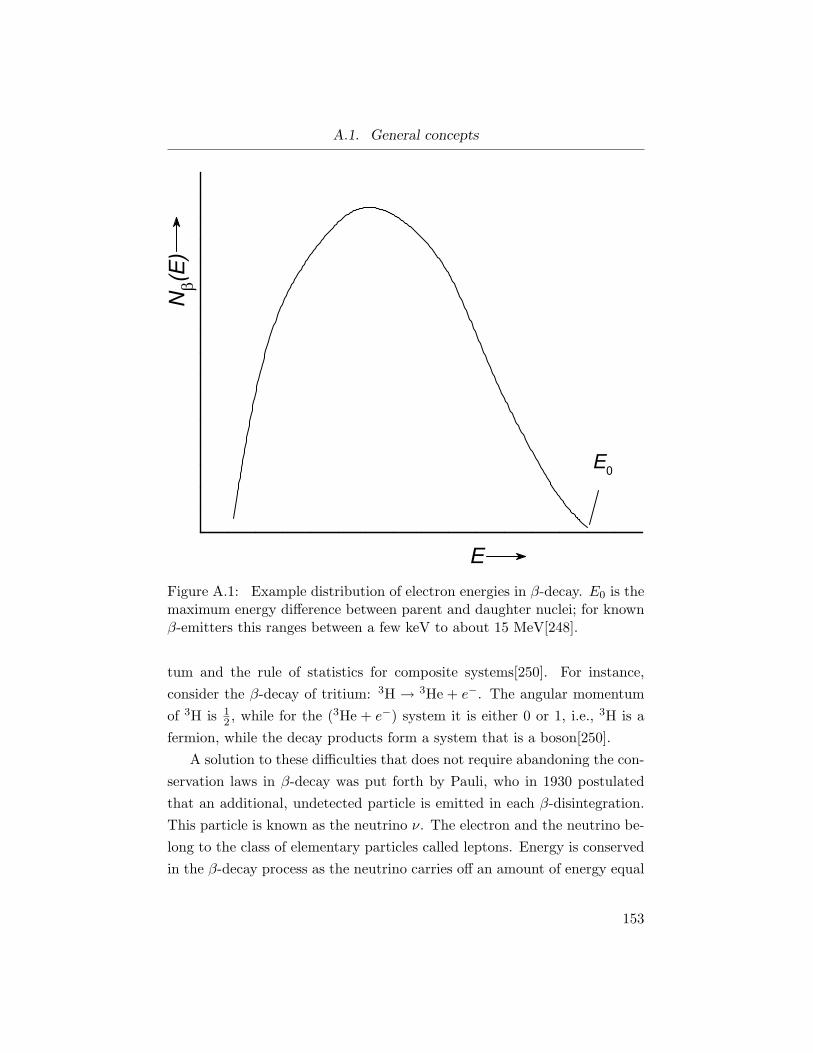
A.1. General concepts
Figure A.1: Example distribution of electron energies in β-decay. E0 is themaximum energy difference between parent and daughter nuclei; for knownβ-emitters this ranges between a few keV to about 15 MeV[248].
tum and the rule of statistics for composite systems[250]. For instance,
consider the β-decay of tritium: 3H → 3He + e−. The angular momentum
of 3H is 12 , while for the (3He + e−) system it is either 0 or 1, i.e., 3H is a
fermion, while the decay products form a system that is a boson[250].
A solution to these difficulties that does not require abandoning the con-
servation laws in β-decay was put forth by Pauli, who in 1930 postulated
that an additional, undetected particle is emitted in each β-disintegration.
This particle is known as the neutrino ν. The electron and the neutrino be-
long to the class of elementary particles called leptons. Energy is conserved
in the β-decay process as the neutrino carries off an amount of energy equal
153
A.1. General concepts
to the difference between the energy of a given β-electron and E0 (except
in EC where the emitted neutrino is monoenergetic)[250]. Additionally, to
preserve charge conservation the neutrino must have a charge of 0 (and thus
an extremely small magnetic moment, if any), and the balance of angular
momentum requires that the neutrino be a spin-12 fermion[250].
The neutrino thus has an associated antiparticle— the antineutrino ν—
with the same spin, charge, and mass as ν[250]. By definition νe is the second
particle emitted in β−-decay,12 and νe is the particle that accompanies β+-
decay and EC[250]. Thus, the elementary processes (i) and (ii) above are
written as:
n → p+ e− + νe (A.1)
p → n+ e+ + νe (A.2)
Free neutrons do decay as shown, and while the free proton is stable, it can
undergo decay inside a nucleus that as a whole can supply the necessary
energy.
The neutrino is a very elusive particle that is hard to detect, but one way
to study the neutrino is to investigate its interaction with other matter such
as in inverse β-decay processes[249, 250]. For instance, the reaction νe+p→n+ e+ was studied by using antineutrinos produced in a nuclear reactor to
bombard a substance containing hydrogen (like H2O). The emitted positrons
are immediately annihilated and the characteristic annihilation radiation is
observed. A small amount of Cd salt was added to the water, and the
emitted neutron is captured by the Cd with the subsequent emission of
characteristic gamma rays ∼ 10−5 s after the e+-annihilation radiation is
detected. This sequence is specific enough to be unambiguous and provided
experimental evidence (in 1953) for the existence of the neutrino[249, 250].
A second particularly important example is the study of the inverse EC
decay of 37Ar: 37Ar + e− → 37Cl + νe. By bombarding 37Cl with νe or νe
12The subscript e has been added to indicate that these neutrinos and antineutrinosare associated with β-decay (the electron); there are also neutrinos and antineutrinosassociated with the decay of the muon and the tau meson that are not identical to thoseemitted in β-decay[248, 249, 250]. This leads to the concept of neutrino “flavour.”
154
A.2. Fermi’s theory of beta decay
produced in a reactor 37Ar should be formed; however, the use of νe gave
a null result, demonstrating νe and νe are two different particles[249, 250].
A distinction between the neutrino and antineutrino is on the basis of their
helicities. The direction of spin of the νe is parallel to its momentum, while
the direction of spin of the νe is antiparallel to its momentum[250]. Thus,
the neutrino helicity is -1, it is a left-handed particle, while the antineutrino
has helicity of +1 and is a right-handed particle[250].
Lastly, the question of the rest mass of the neutrino mν is of fundamen-
tal significance to nuclear and astrophysics problems, more so than for beta
decay. Experimentally, precise measurements of mν are very difficult, and
only upper and lower limits are determined[249]. For many years, mν was
taken to be exactly zero[250]; however, it is now believed that mν is different
from zero, but still very tiny, e.g., < 20 eV/c2[249], or 0.00004 times the elec-
tron rest mass. The notion of a non-zero neutrino rest mass originated from
experiments designed to measure the flux of neutrinos originating from the
sun’s nuclear reactions that strike earth. The results of these measurements
(starting with R. Davis’ pioneering Homestake Mine experiment and later
supplemented/augmented by data from (Super)Kamiokande and the Sud-
bury Neutrino Observatory) supported theories proposed as early as 1969
that the (anti)neutrino can undergo oscillations in flavour[249], e.g., νµ → νe
(see footnote 12). For this to be the case the neutrino can not be truly
relativistic— it must have a finite rest mass. The value of mν has impor-
tant consequences for profound questions in cosmology, like (anti)neutrino
production during the Big Bang and other tests of models of the origin of
the universe[249].
A.2 Fermi’s theory of beta decay
Fermi formulated a quantitative theory of β-decay that includes Pauli’s (then
hypothetical) neutrino in 1934[248]. In 1957 experimental observations (see
following Section) required Fermi’s theory be modified[249], but many of his
results remained valid[250] and the theory provides the foundation for the
understanding of β-decay. The fundamental interaction that governs the
155
A.2. Fermi’s theory of beta decay
beta decay process is the weak interaction. By 1933 the quantum theory
of radiation was well established, so Fermi formulated his β-decay theory
by analogy with the electromagnetic interaction[248, 249, 250]. Just as
photons are created at the time of emission as a nucleus or molecule passes
from an excited state to the ground state, β±-particles and (anti)neutrinos
are created as the nucleus decays. Fermi’s theory provides a dynamical
description of this process explaining the shape of beta spectra (e.g., Fig.
A.1), the relation between E0 and the mean lifetime of the nucleus, and
allows β-decay transitions to be classified on the basis of selection rules[250].
Using time-dependent perturbation theory, the starting point for the
β-decay transition rate λ is Fermi’s golden rule
λ =2π
h|Hfi|2ρ, (A.3)
where Hfi is the weak interaction Hamiltonian matrix element between the
final and initial states, and ρ = dN/dE0 is the density of the final states,
i.e., the number of final states per unit of total decay energy (the “phase
space” term). Here, λ represents the total probability per unit time that a
β-particle is emitted. A detailed mathematical treatment can be found in
Ref. [250]. The final expression is
λ =g2m5
ec4
2π3h7 |Mfi|2f(Z, ǫ0), (A.4)
where g is a constant, Mfi is a number that stems from the overlap integral
over the parent and daughter nuclear wavefunctions. The function f(Z, ǫ0),
where ǫ0 = E0/mec2, is known as the Fermi function. It gives a correction
for the Coulomb interaction between the nucleons of the daughter nuclei and
the emitted electron. It gives rise to distortions of the β spectrum from an
otherwise “bell-shape”[249] mostly near the maximum energy region (e.g.,
Fig. A.1).
By defining a mean lifetime for the decaying nucleus as τ ≡ λ−1, and
noting that the half-life t 12
of the decaying nucleus is given by t 12
= τ ln 2,
156
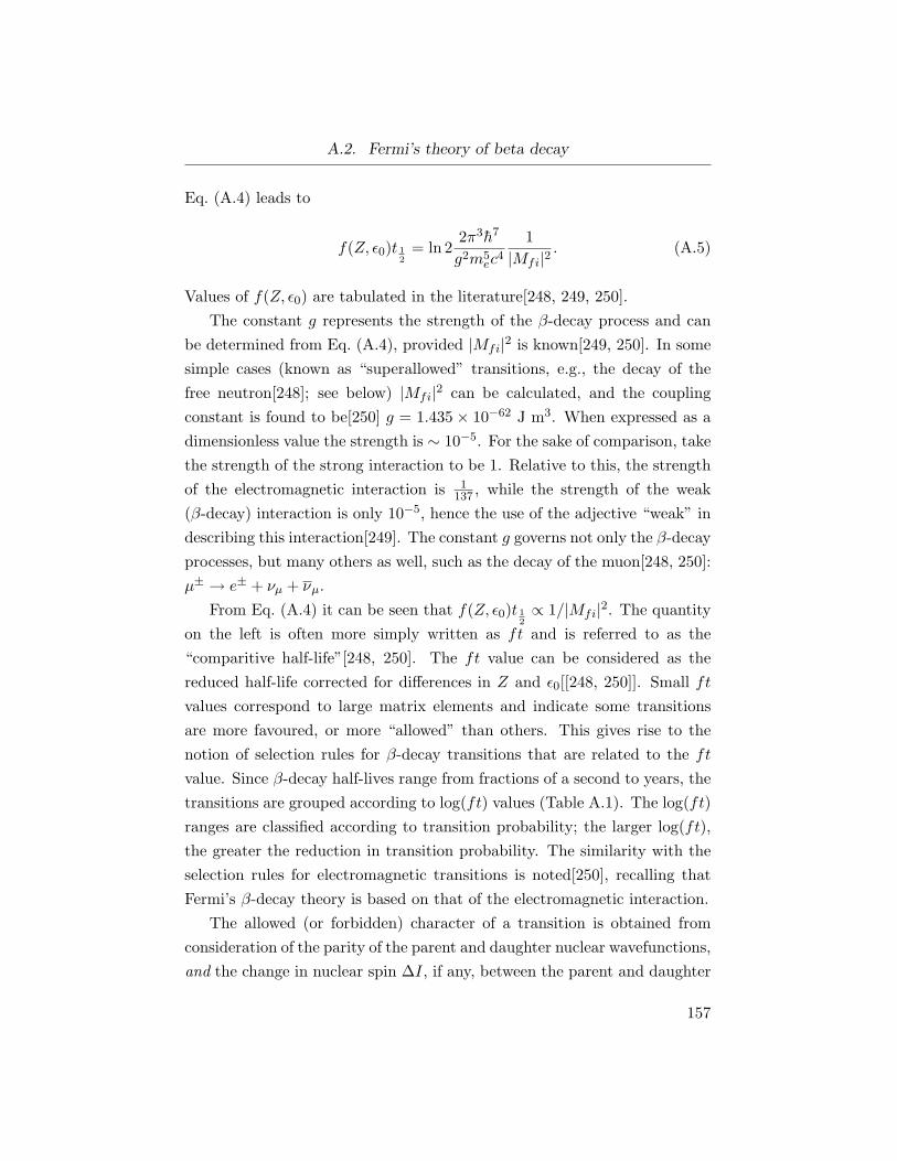
A.2. Fermi’s theory of beta decay
Eq. (A.4) leads to
f(Z, ǫ0)t 12
= ln 22π3h7
g2m5ec
4
1
|Mfi|2. (A.5)
Values of f(Z, ǫ0) are tabulated in the literature[248, 249, 250].
The constant g represents the strength of the β-decay process and can
be determined from Eq. (A.4), provided |Mfi|2 is known[249, 250]. In some
simple cases (known as “superallowed” transitions, e.g., the decay of the
free neutron[248]; see below) |Mfi|2 can be calculated, and the coupling
constant is found to be[250] g = 1.435 × 10−62 J m3. When expressed as a
dimensionless value the strength is ∼ 10−5. For the sake of comparison, take
the strength of the strong interaction to be 1. Relative to this, the strength
of the electromagnetic interaction is 1137 , while the strength of the weak
(β-decay) interaction is only 10−5, hence the use of the adjective “weak” in
describing this interaction[249]. The constant g governs not only the β-decay
processes, but many others as well, such as the decay of the muon[248, 250]:
µ± → e± + νµ + νµ.
From Eq. (A.4) it can be seen that f(Z, ǫ0)t 12∝ 1/|Mfi|2. The quantity
on the left is often more simply written as ft and is referred to as the
“comparitive half-life”[248, 250]. The ft value can be considered as the
reduced half-life corrected for differences in Z and ǫ0[[248, 250]]. Small ft
values correspond to large matrix elements and indicate some transitions
are more favoured, or more “allowed” than others. This gives rise to the
notion of selection rules for β-decay transitions that are related to the ft
value. Since β-decay half-lives range from fractions of a second to years, the
transitions are grouped according to log(ft) values (Table A.1). The log(ft)
ranges are classified according to transition probability; the larger log(ft),
the greater the reduction in transition probability. The similarity with the
selection rules for electromagnetic transitions is noted[250], recalling that
Fermi’s β-decay theory is based on that of the electromagnetic interaction.
The allowed (or forbidden) character of a transition is obtained from
consideration of the parity of the parent and daughter nuclear wavefunctions,
and the change in nuclear spin ∆I, if any, between the parent and daughter
157
A.2. Fermi’s theory of beta decay
Table A.1: General classification of beta decay transitions[249].
Type log(ft)
Superallowed ∼ 3Allowed 4–6First forbidden 6–10Second forbidden 10–13Third forbidden > 15Fourth forbidden[248] ∼ 23
nuclei. Thus, for β-decay, wavefunction parity and angular momentum form
the basis of the selection rules.
The first aspect arises because integrals in |Mfi|2 over the parent and
daughter wavefunctions have non-zero overlap only if the parity of the wave-
functions is unchanged, and vice-versa[249]. The second aspect arises in
considering restrictions on the value of the total angular momentum of
the leptons, recalling both the electron and neutrino have intrinsic spin
of 12 . The transition probability is greatest when the lepton wavefunctions
at the position of the nucleus [ψe(0) and ψν(0)] that enter into Hfi have
the greatest magnitude. A wavefunction of orbital angular momentum l
behaves as (Rn/λeC)l near the origin[251], where Rn is the nuclear radius
(∼ 10−15 m) and λeC is the Compton wavelength of the electron (3.9×10⁻¹³
m). Thus, the probability that the emitted leptons carry orbital angular
momentum is small and decreases rapidly with increasing l. The lepton
wavefunctions will be greatest at the origin for l = 0 when the leptons are
emitted with zero orbital angular momentum, i.e., “s-wave state” electrons
and (anti)neutrinos[248, 250]. However, for a relativistic particle, l is not a
constant of motion, but j the total angular momentum is[250]. The most
allowed transitions therefore occur when the leptons are emitted with a
minimum of orbital angular momentum je = jν = 12 [251].
The total amount of angular momentum carried away by the electron
and the neutrino is 0 if they are emitted with spins antiparallel, and it is 1
if they are emitted with spins parallel[250]. The former is a singlet state,
158
A.2. Fermi’s theory of beta decay
while the latter is a triplet state. In the case of singlet lepton emission the
spin of the nucleus cannot change, so
∆I = 0 (A.6)
without a change of wavefunction parity. This selection rule was proposed
by Fermi, F-transition[248, 249, 250]. If the leptons are emitted in a triplet
state
∆I = ±1, 0, but 0 → 0 forbidden (A.7)
again without a change in wavefunction parity. This selection rule was
proposed by G. Gamow and E. Teller, GT-transition[248, 249, 250].
The F and GT selection rules are not mutually exclusive[250]. For in-
stance, the decay of the free neutron mentioned above is a 12
+ → 12
+tran-
sition (Ii = If 6= 0; ∆I = 0) and so a mixture of F and GT processes
contribute. Thus, in lowest order[249] |Mfi|2 = |Mfi(F)|2 +g2GT
g2F|Mfi(GT)|2.
The 0+ → 0+ superallowed decays are uniquely F-transitions, and from their
study gF = g can be determined[249]. From the best determinations of the
coupling constant strengths gGTgF
= −1.259(4)[249].
The transitions classified as forbidden take place via the emission of
non-s-state leptons[248], because l cannot be restricted to zero[251]. The
emission of leptons with non-zero orbital angular momentum arises from
the fact that they are not emitted from a point source, but rather the finite
volume of the nucleus must be considered. The wavefunctions ψe(0) and
ψν(0) must be evaluated over the entire nuclear volume and this introduces
p-,d, and higher-wave states into the emission[248, 250]. As stated above,
as l increases, the probability of the β-transition rapidly decreases, and so
transitions with l = 1, 2, 3, . . . are classified as first, second, third,. . . for-
bidden transitions[248]. These transitions require that higher order terms
be considered in the expansion of the plane waves used for the lepton wave-
functions
eik·r = 1 + ik · r − (k · r)2
2+ · · · . (A.8)
Thus, the second term in Eq. (A.8) corresponds to l = 1, and if it is this term
159
A.3. Parity violation in beta decay
that is important in the interaction causing the transition, the leptons are
emitted in a p-wave state; the parent and daughter nuclei must have opposite
parity[248, 250]. The higher order terms of the plane waves introduce powers
of pe and pν into the matrix element[250]. Consequently, the matrix element
is no longer independent of the energy partition between the electron and
the (anti)neutrino (as it is for allowed transitions)[248], and so the shape of
the β spectrum for forbidden transitions is different from that of the typical,
allowed Fermi spectrum[250].
A.3 Parity violation in beta decay
The nonconservation of parity in β-decay was an important discovery and is
an aspect of this type of radioactive decay that is crucial to the implemen-
tation of the β-NMR technique. Processes governed by the weak interaction
(like β-decay) have nonconservation of parity in common, and this is a ma-
jor distinction between the weak interaction and the electromagnetic and
strong interactions as parity is conserved for processes involving the latter
two alone[250]. Parity (non)conservation can be described at various lev-
els of sophistication. One simple description is that if the mirror image
of a phenomenon is also a physically realizable phenomenon, then parity is
conserved[250]. Thus, parity conservation implies space-reflection symmetry
holds for a given phenomenon.
Consideration of space-reflection symmetry to the β-decay process re-
quires the distinction of two types of vector quantities. Space-reflection of
a given point is equivalent to inversion of the coordinates through the ori-
gin, i.e., (x, y, z) → (−x,−y,−z)[248, 250]. Vectors for which this change
of sign of space coordinates occurs are called “polar” vectors, examples
of which are linear momentum and electric field[248, 250]. On the other
hand, vectors such as angular momentum or magnetic field are character-
ized not only by direction, but also by a screw sense or handedness, and
they do not change sign under inversion[248, 250]. Vectors of this second
type are termed “axial” vectors (or “pseudovectors”).13 The product of any
13Axial vectors do not change sign because they are the result of the cross-product of
160
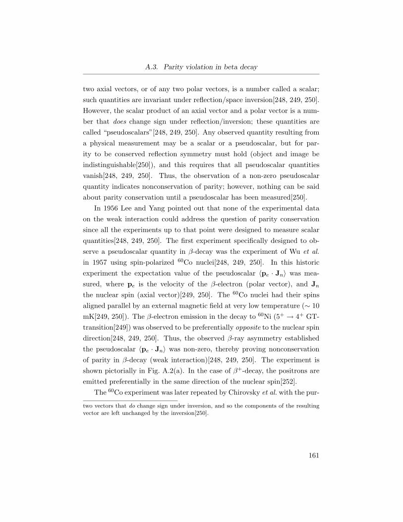
A.3. Parity violation in beta decay
two axial vectors, or of any two polar vectors, is a number called a scalar;
such quantities are invariant under reflection/space inversion[248, 249, 250].
However, the scalar product of an axial vector and a polar vector is a num-
ber that does change sign under reflection/inversion; these quantities are
called “pseudoscalars”[248, 249, 250]. Any observed quantity resulting from
a physical measurement may be a scalar or a pseudoscalar, but for par-
ity to be conserved reflection symmetry must hold (object and image be
indistinguishable[250]), and this requires that all pseudoscalar quantities
vanish[248, 249, 250]. Thus, the observation of a non-zero pseudoscalar
quantity indicates nonconservation of parity; however, nothing can be said
about parity conservation until a pseudoscalar has been measured[250].
In 1956 Lee and Yang pointed out that none of the experimental data
on the weak interaction could address the question of parity conservation
since all the experiments up to that point were designed to measure scalar
quantities[248, 249, 250]. The first experiment specifically designed to ob-
serve a pseudoscalar quantity in β-decay was the experiment of Wu et al.
in 1957 using spin-polarized 60Co nuclei[248, 249, 250]. In this historic
experiment the expectation value of the pseudoscalar 〈pe · Jn〉 was mea-
sured, where pe is the velocity of the β-electron (polar vector), and Jn
the nuclear spin (axial vector)[249, 250]. The 60Co nuclei had their spins
aligned parallel by an external magnetic field at very low temperature (∼ 10
mK[249, 250]). The β-electron emission in the decay to 60Ni (5+ → 4+ GT-
transition[249]) was observed to be preferentially opposite to the nuclear spin
direction[248, 249, 250]. Thus, the observed β-ray asymmetry established
the pseudoscalar 〈pe · Jn〉 was non-zero, thereby proving nonconservation
of parity in β-decay (weak interaction)[248, 249, 250]. The experiment is
shown pictorially in Fig. A.2(a). In the case of β+-decay, the positrons are
emitted preferentially in the same direction of the nuclear spin[252].
The 60Co experiment was later repeated by Chirovsky et al. with the pur-
two vectors that do change sign under inversion, and so the components of the resultingvector are left unchanged by the inversion[250].
161
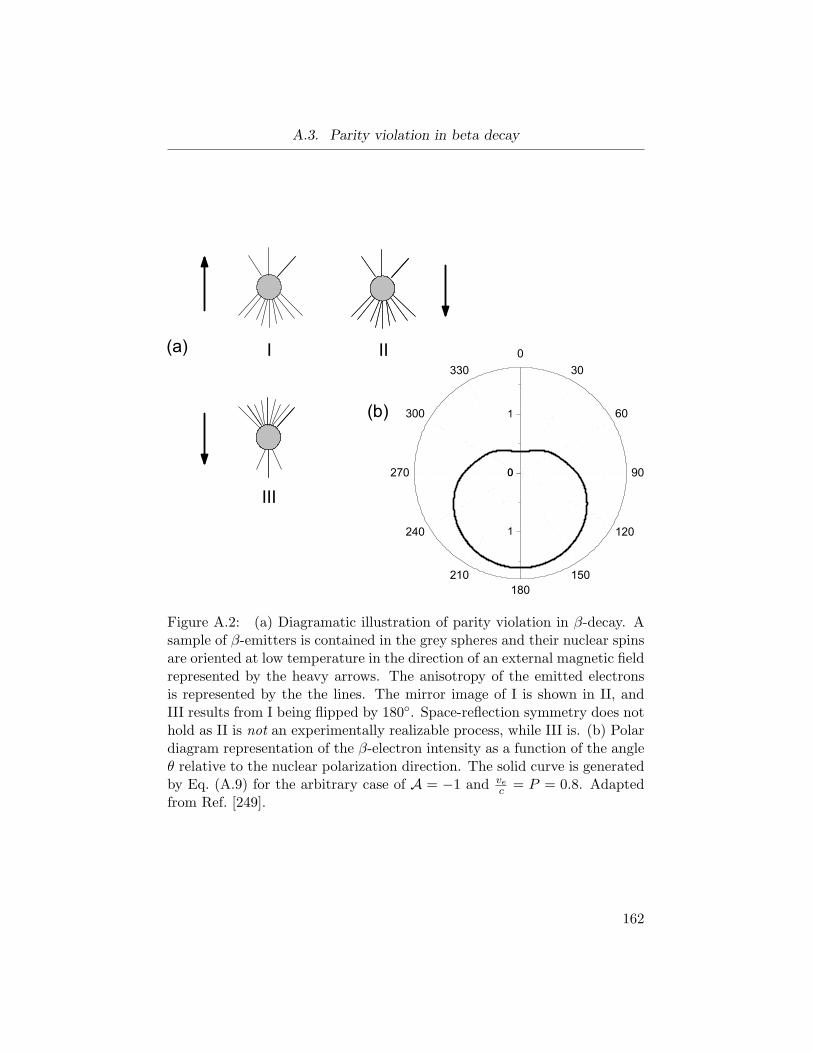
A.3. Parity violation in beta decay
Figure A.2: (a) Diagramatic illustration of parity violation in β-decay. Asample of β-emitters is contained in the grey spheres and their nuclear spinsare oriented at low temperature in the direction of an external magnetic fieldrepresented by the heavy arrows. The anisotropy of the emitted electronsis represented by the the lines. The mirror image of I is shown in II, andIII results from I being flipped by 180◦. Space-reflection symmetry does nothold as II is not an experimentally realizable process, while III is. (b) Polardiagram representation of the β-electron intensity as a function of the angleθ relative to the nuclear polarization direction. The solid curve is generatedby Eq. (A.9) for the arbitrary case of A = −1 and ve
c = P = 0.8. Adaptedfrom Ref. [249].
162
A.3. Parity violation in beta decay
pose of measuring the angular asymmetry of the β-electron distribution[253]
Nβ(θ) = 1 + AP (ve
c) cos θ. (A.9)
Nβ(θ) stands for the β-electron intensity as a function of the angle θ with
respect to the nuclear polarization vector, vec is the ratio of the velocity
of the β-electron to the speed of light, P the polarization of the nuclei,
and A is the beta-spin correlation or asymmetry coefficient. The parameter
A depends on the parent nucleus, i.e., the specific interaction causing the
decay[250]. For the case of 60Co, Atheory = −1, and the experimental results
are in excellent agreement, giving Aexp = −1.01(2)[253]. As an illustration
of the directional anisotropy of the β-radiation from an oriented nucleus,
Nβ(θ) is shown in Fig. A.2(b) for A = −1 and 0.8 for the other two terms.
The fundamental origin of parity violation is still not fully understood, and
β-decay experiments continue to provide details into parity violation for the
weak interaction[252]. Experiments of the type described above for 60Co
are usually conducted using a β-source in the form of a solid sample, and
as such are limited in precision due to effects of scattering or magnetic
deflection on the β-particle trajectories[252, 253]. Modern experiments aim
to overcome this limitation by using magneto-optic traps to confine “clouds”
of spin polarized β-active atoms, thereby allowing quantities such as A to
be extracted with even greater precision[252]. Since the 60Co experiment of
Wu et al. several other experiments have corroborated nonconservation of
parity in the weak interactions; for these processes nature can distinguish
between right and left[248].
Parity-nonconserving terms were omitted from the Hamiltonians for the
weak interactions until experiment showed they must be included[250], high-
lighting the historical importance of such experiments. It was by analogy to
the strong and electromagnetic interactions that these terms were initially
omitted[250]. For instance, in equations for the energy of the electromag-
netic field, scalar terms such as H2 and E2 are allowed, but a term such as
H ·E is a pseudoscalar which is not permissible (as it would change sign un-
der inversion)[250]. As mentioned, Fermi constructed his theory of β-decay
163
A.4. Decay of 8Li
by analogy to the electromagnetic interaction, and so the theory described in
Sec. A.2 is formulated on the assumption that parity is conserved[250]. How-
ever, it is important to note that the main results of Fermi’s theory regarding
β spectra shapes and lifetimes are essentially unaffected by the nonconserva-
tion of parity since his calculations involve only scalar quantities[248, 250].
A.4 Decay of 8Li
The β-emitter 8Li is used for the present β-NMR experiments. Some phys-
ical properties of this nucleus are given in Table A.2. It decays according
to8Li →8 Be + e− + νe. (A.10)
The ground state of the 8Li nucleus is of spin 2+ and it decays to a 2+ ex-
cited state of 8Be that is situated 2.9 MeV above its ground state[254]. This
decay is thus allowed by both F and GT selection rules (Sec. A.2); however,
as discussed below, it is dominated by the strength of the GT coupling[254].
The value of E0 for this decay is 13.1 MeV and log(ft) = 5.4[254], and is
thus an “allowed” transition. An advantage in using 8Li for β-NMR experi-
ments is that the high energy β-electrons are easy to discriminate from low
energy background radiation[254].
The excited daughter 8Be nucleus can relax to the ground state by the
emission of gamma radiation, after which it promptly disintegrates into two
α-particles (42He nuclei). The 8Be → 2α decay is termed “prompt” as t 12
is
just 7 × 10⁻¹⁷ s[255]. This means the daughter nuclei do not remain in the
sample which is another advantage of using 8Li for β-NMR.
The ground state of 8Li is a member of the isospin triplet: 8Li, 8Be,8B[254]. The concept of isospin (or isobaric spin) T is used in nuclear struc-
ture models and is based on the idea that the force acting on the proton
and neutron is independent of charge and therefore the two nucleons can be
considered as different quantum states of a single particle[248]. This is anal-
ogous to the quantum mechanical description of the two spin states of the
electron, i.e., “spin-up” or “spin-down.” Just as the electron may be assigned
164
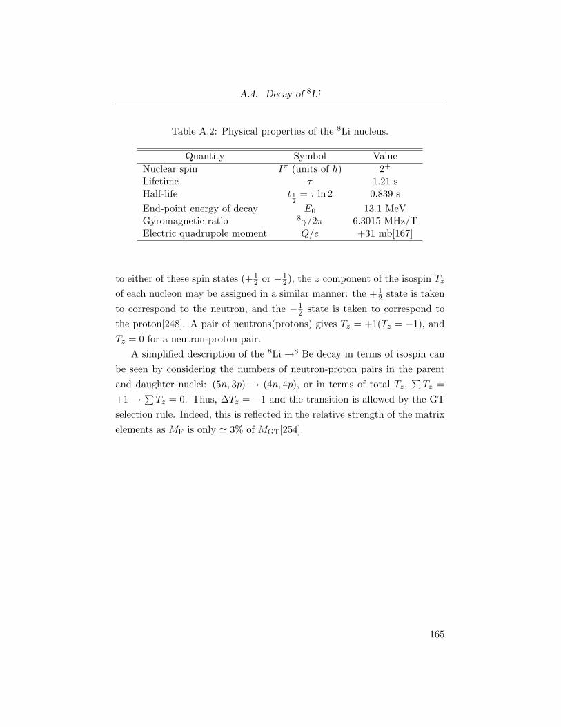
A.4. Decay of 8Li
Table A.2: Physical properties of the 8Li nucleus.
Quantity Symbol Value
Nuclear spin Iπ (units of h) 2+
Lifetime τ 1.21 sHalf-life t 1
2= τ ln 2 0.839 s
End-point energy of decay E0 13.1 MeVGyromagnetic ratio 8γ/2π 6.3015 MHz/TElectric quadrupole moment Q/e +31 mb[167]
to either of these spin states (+12 or −1
2), the z component of the isospin Tz
of each nucleon may be assigned in a similar manner: the +12 state is taken
to correspond to the neutron, and the −12 state is taken to correspond to
the proton[248]. A pair of neutrons(protons) gives Tz = +1(Tz = −1), and
Tz = 0 for a neutron-proton pair.
A simplified description of the 8Li →8 Be decay in terms of isospin can
be seen by considering the numbers of neutron-proton pairs in the parent
and daughter nuclei: (5n, 3p) → (4n, 4p), or in terms of total Tz,∑
Tz =
+1 → ∑
Tz = 0. Thus, ∆Tz = −1 and the transition is allowed by the GT
selection rule. Indeed, this is reflected in the relative strength of the matrix
elements as MF is only ≃ 3% of MGT[254].
165
Appendix B
Ion Implantation in Metals
B.1 General concepts of ion implantation in
solids
The processes governing the implantation of ions into solids (or passage
through them at sufficient energies) are complex, but generally well-understood
as this subject has been intensely studied since the early twentieth century[256,
257]. The earliest theoretical considerations of the stopping (slowing down)
of a projectile ion into a solid have evolved into modern computer simula-
tion programs that are both fast and quite accurate. Experiments on the
stopping of ions in solids provided data with which to test theories or aid
in computer simulation, and have given way to two major technological ap-
plications of ion implantation: microanalysis and controllable modification
of materials. Ion implantation allows for reproducible modification of sur-
face and near-surface properties of materials and is used frequently in device
fabrication. For example, it can be used to form alloys of desired composi-
tions without the loss of crystal structure and does not suffer from potential
miscibility problems associated with other alloying techniques[258]. An im-
portant example is the introduction of selective concentrations of dopant
atoms into semiconductors. On the other hand, high-energy ion bombard-
ment of materials can be employed to impart desired degrees of disorder to a
crystal, transform a crystalline lattice into a fully amorphous state, or create
regions of intermixing at the interface of two dissimilar crystals[258]. Ion
implantation can also be used to create nanometer sized clusters embedded
in various hosts to form nanocomposite materials[259], while both ion im-
plantation and irradiation can be employed for topographical patterning of
166
B.1. General concepts of ion implantation in solids
materials[260]. Ion beams— especially those of protons or α particles— are
also used to analyze the composition of materials as a function of depth be-
low the surface, for example, Rutherford backscattering spectrometry[261].
The 8Li ions used in these β-NMR experiments do not remain in the sam-
ples (nor do the daughter nuclei; see Appendix A); however, the processes
by which they lose energy and eventually stop in the hosts are important to
consider. In this Appendix, the mechanisms of ion implantation are briefly
summarized— mostly qualitatively. As well, the possible types of damage
that may be produced during the implantation are summarized. In the final
Section the computer simulation program TRIM.SP that has been used to
obtain the 8Li+ stopping distributions for the studies in this thesis is re-
viewed. In keeping with the topic of this thesis, the present survey focuses
on implantation into metallic hosts.
Two important aspects to consider are the scattering of the projectile ion
by collisions with the host atoms, and the energy transferred from the former
to the latter. These in turn affect the overall path length (i.e., mean stopping
depth) of the implanted ion, and the degree of damage to the host. The two
major modes of energy loss for the incident ions are the direct collisions
with the host nuclei, and the excitation of the electrons of the host. Both
of these processes are energy-dependent and so make varying contributions
along the path of the ion x: (dE/dx)loss = (dE/dx)nucl + (dE/dx)elec. An
overview of these two processes is given next, then more details are provided
in regards to the particular computer simulation program employed here.
The dominant mode of energy loss for implanted ions with energies less
than ∼ 0.5 MeV (pertinent to β-NMR) is through the elastic interactions
with the target nuclei. These nuclear collisions give rise to “Rutherford
scattering” as the electrostatic Coulomb repulsion from the screened nucleus
will deflect the ion. Being elastic in nature, both energy and momentum are
conserved, and these collisions are treated as two body events in a centre-
of-mass coordinate system. The important parameters being the energy
lost by the impinging ion, the cross-section for the energy transfer, and the
scattering angle Θ. If the mass of the impinging and target atoms differs
significantly, the scattering angle is small.
167
B.1. General concepts of ion implantation in solids
An important consideration in the evaluation of nuclear collision events
is the choice of the interatomic potential V (r), where r is the interatomic
separation. This repulsive potential is chosen such that the particles can
be assigned a definite radius, and thus predict Θ. The earliest treatments
used analytical expressions for V (r), typically containing a 1/r Coulombic
term multiplied by a screening term. As there is no definitive expression for
V (r) that is appropriate for all ion pairs at all energies, these functions are
often modified through the addition of empirically adjustable parameters.
With the advent of the computer, descriptions of V (r) spanning a wide
range of r can now be made numerically. Both head-on and glancing angle
collisions are considered by defining a total cross-section for energy transfer;
the probability of energy transfer (loss) for a given scattering angle can then
be related to the total cross-section.
The electronic energy losses occur through inelastic interactions with the
electron clouds of the target. As the energy of the impinging ion increases,
the energy loss due to elastic (nuclear) collisions decreases (essentially ∝1/E), and the inelastic (electronic) events dominate. At high velocities, the
projectile ion is fully stripped of its electrons. This occurs when the ion’s
velocity is greater than the Bohr velocity of the target atom electrons. In
this regime, the rate of energy loss is related to the closeness of the ion to the
target atoms and thereby the number of electronic excitations it can produce,
i.e., proportional to the degree of “penetration” through the target electron
shells. The electronic energy losses do not cause significant deflection of
the ion. It is emphasized that this type of energy loss is important for ion
energies greater than hundreds of keV/amu, and so makes little contribution
to the much lower energy 8Li+ stopping in the studies of this thesis.
Upon considering the above mechanisms for energy loss of a projectile
ion, the total distance (path length) travelled by the ion until it is brought
to rest in a given target can be predicted. This is expressed through the
mean range R and the range straggling ∆R. First, it is noted that overall
a crystalline target may be treated in a similar fashion as an amorphous
one. The reason for the similarity is because the range is determined by
averaging over many individual events. The range is defined as the mean
168
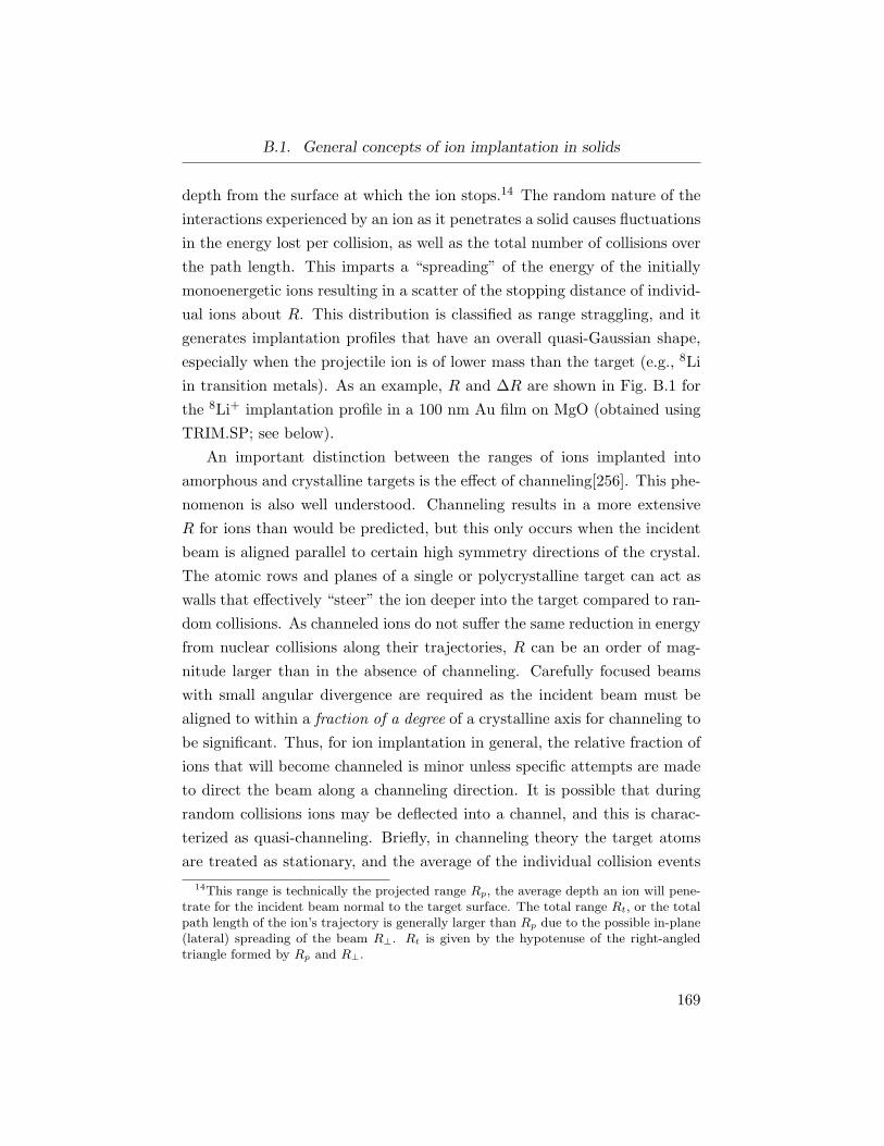
B.1. General concepts of ion implantation in solids
depth from the surface at which the ion stops.14 The random nature of the
interactions experienced by an ion as it penetrates a solid causes fluctuations
in the energy lost per collision, as well as the total number of collisions over
the path length. This imparts a “spreading” of the energy of the initially
monoenergetic ions resulting in a scatter of the stopping distance of individ-
ual ions about R. This distribution is classified as range straggling, and it
generates implantation profiles that have an overall quasi-Gaussian shape,
especially when the projectile ion is of lower mass than the target (e.g., 8Li
in transition metals). As an example, R and ∆R are shown in Fig. B.1 for
the 8Li+ implantation profile in a 100 nm Au film on MgO (obtained using
TRIM.SP; see below).
An important distinction between the ranges of ions implanted into
amorphous and crystalline targets is the effect of channeling[256]. This phe-
nomenon is also well understood. Channeling results in a more extensive
R for ions than would be predicted, but this only occurs when the incident
beam is aligned parallel to certain high symmetry directions of the crystal.
The atomic rows and planes of a single or polycrystalline target can act as
walls that effectively “steer” the ion deeper into the target compared to ran-
dom collisions. As channeled ions do not suffer the same reduction in energy
from nuclear collisions along their trajectories, R can be an order of mag-
nitude larger than in the absence of channeling. Carefully focused beams
with small angular divergence are required as the incident beam must be
aligned to within a fraction of a degree of a crystalline axis for channeling to
be significant. Thus, for ion implantation in general, the relative fraction of
ions that will become channeled is minor unless specific attempts are made
to direct the beam along a channeling direction. It is possible that during
random collisions ions may be deflected into a channel, and this is charac-
terized as quasi-channeling. Briefly, in channeling theory the target atoms
are treated as stationary, and the average of the individual collision events
14This range is technically the projected range Rp, the average depth an ion will pene-trate for the incident beam normal to the target surface. The total range Rt, or the totalpath length of the ion’s trajectory is generally larger than Rp due to the possible in-plane(lateral) spreading of the beam R⊥. Rt is given by the hypotenuse of the right-angledtriangle formed by Rp and R⊥.
169
B.1. General concepts of ion implantation in solids
Figure B.1: Stopping profile for 13 keV 8Li+ implanted into a 100 nmAu film on MgO. The mean range R = 44 nm, and the range straggling∆R ∼ ±25 nm. The small peaks in the curve are numerical noise due to therelatively small number of particles used in the simulation (1 × 10⁴).
170
B.1. General concepts of ion implantation in solids
is treated by replacing the rows of atoms by a continuous potential; yet,
precise predictions of R for channeled ions is difficult. Empirical corrections
to R determined for amorphous targets are often necessary.
B.1.1 Damage produced by ion implantation
As stated above, during the elastic nuclear collisions a projectile ion will
scatter off of the target atoms, and in doing so transfer some of its kinetic
energy to them over the length of the implantation trajectory, as well as
generate local heating. The energy may be sufficient to displace an atom of
the target material, disrupting the atomic order and impart some degree of
disorder to the lattice[188, 256]. This perturbation caused by the implanted
ion is referred to as radiation damage. The response of the target lattice is a
dynamic event, and at a given temperature, the perturbed atoms may rear-
range (relax) into various defect structures. Often these radiation-induced
defects may result in superior mechanical properties for a given material over
the original lattice, and may be thermodynamically difficult to produce by
other processing techniques. The disordered region is limited to the region
surrounding the implantation track. Just as the ranges of ions in solids have
been extensively studied for many years, so too have the effects of radiation
damage.
There are two broad classes of defects that result from radiation damage.
The first involves one or two disrupted target atoms. These are therefore
analogous to the point defects encountered normally in solids, i.e., vacancies
and interstitials. A vacancy is simply a missing atom (or ion) in a lattice,
and at finite T , there is always a thermodynamic equilibrium concentration
of such vacancies in otherwise “perfect” crystals as the entropy of the lattice
is increased by the presence of disorder[3]. For metals the energy required
to form a monovacancy Efv1 is typically 1 – 2 eV. As specific examples, Ef
v1
for Au is ∼ 0.9 eV, while for Pd it is ∼ 1.8 eV. The probability of a va-
cant lattice site is given by the Boltzmann factor at thermal equilibrium[3]
(exp[−Efv1/kBT ]). For Ef
v1 = 1 eV at 1000 K, the equilibrium concentration
of vacancies is ≃ 10−5, which for one mole of atoms is ∼ 1018 lattice sites.
171
B.1. General concepts of ion implantation in solids
There are two types of vacancy defects: (i) the Schottky defect is a lattice
vacancy in which the missing atom is considered to be transferred to the sur-
face of the crystal; (ii) in the Frenkel defect the missing atom is moved into
an interstitial lattice site not normally occupied by an atom. For this latter
defect the vacancy-interstitial pair thus remain in the bulk of the crystal.
The interstitial is an important defect as it perturbs the surrounding lattice
rather strongly and can significantly affect bulk properties. Vacancies also
provide a means for thermally-activated atomic transport in pure materials.
Much of the knowledge of the properties and behaviour of complex de-
fects in metals has come from the study of point defects. Since vacancies can
be formed at high temperatures, they may be studied under thermal equilib-
rium conditions by heating a sample, often to just below the melting point.
The high temperature concentration can then by quenched, or “frozen” into
the sample by rapid cooling. Point defects produced by quenching or ir-
radiation are formed under non-equilibrium conditions and are metastable
as they can be thermally annealed out of the sample. At certain tempera-
tures particular defects begin to migrate and can form complexes, undergo
annihilation reactions, or become trapped at grain boundaries, dislocations,
impurity atoms, etc. In simple metals, the interstitial defect generally be-
comes mobile at low temperatures (less than about 50 K), while for vacancies
this is nearer to room temperature.
A vast amount of data on the annealing properties of defects in met-
als has come from measurements of the electrical resistivity. The “recovery
curves” for many metals exhibit general features that are quite similar. Us-
ing copper as the prototype, the annealing of metals has been divided into
three principle characteristic stages, that are subdivided into five (I–V). It
should be noted that annealing of defects in insulators often corresponds to
these stages as well; however, in non-metallic systems, the charge state of
the lattice plays an important role in defect formation and stability. For
example, stage I (which itself is subdivided into five stages) is described by
interstitial migration and recombination with vacancies, while stage III cor-
responds to vacancy migration and agglomeration. Finally, although much
information has been obtained from resistivity measurements, techniques
172
B.2. Simulations of 8Li+ implantation profiles using TRIM.SP
like NMR, X-ray spectroscopy, and electron microscopy have further con-
tributed to the understanding of defect formation and dynamics.
The collisions between a projectile ion and the target atoms often result
in the displacement of the target atom from its regular lattice site creating
an interstitial and a vacancy, i.e., a Frenkel defect, or what is commonly
called a Frenkel pair. The displaced atom is referred to as the primary
knock-on atom (PKA), and it may in turn lose the energy transferred to
it by displacing other target atoms from their lattice sites. This gives rise
to the concept of “radiation damage cascades.” However, because these
damage cascades are formed under dynamic, non-equilibrium conditions,
the target lattice may not relax and the energy required to displace an
atom is greater than the equilibrium Efv1. Instead, the threshold energy for
atom displacement Ed must be considered. For most metals Ed is usually
in the range of ≈ 20–50 eV, and it is frequently both temperature- and
orientation-dependent[262, 263]. Values of Ed are directly measureable using
high voltage electron microscopy. If the energy transferred to a PKA is
less than Ed, the atom is not displaced and the energy goes into lattice
vibrations.
B.2 Simulations of 8Li+ implantation profiles
using TRIM.SP
Computer simulations of ion implantation based on the binary collision ap-
proximation using Monte Carlo calculations are available that can yield ion
range distributions for multilayered targets over a wide energy range[257].
One such program is TRIM (TRansport of Ions in Matter). A variation
of this code called TRIM.SP (the SP stands for sputtering)[265] has been
used to obtain the 8Li+ stopping distributions for the β-NMR studies in this
thesis. In this Section a brief summary of the basics of the TRIM method-
ology is given[264]. The program provides high computer efficiency without
sacrificing accuracy. It uses a specially developed analytical formulae to ac-
count for the nuclear scattering. As it uses a Monte Carlo method it can
173
B.2. Simulations of 8Li+ implantation profiles using TRIM.SP
more rigorously treat the elastic scattering events and explicitly treat sur-
faces and interfaces (the latter two being difficult to account for in analytical
treatments based on transport theory).
The simulations consist of following a large number of individual ions
(particles) in a specified target. These are referred to as “histories.” For each
history a particle is assigned an energy, a direction and starting position.
The path of the particles is changed as a result of nuclear collisions, while
they are assumed to move in straight free-flight paths between collisions.
The particles lose energy as a result of the nuclear and electronic mecha-
nisms, and the program is valid for incident ions with energies in the range of
0.1 keV to several MeV. TRIM considers the target to be completely amor-
phous with atoms in random positions (but maintaining a density specified
by the user), and so can not account for things such as channeling, isotopic
distributions, or variations in stoichiometry (where applicable). Recall that
overall range distributions for crystalline and amorphous materials are simi-
lar as it is the average of many particles undergoing many random collisions
that is important. The program provides data on implanted, reflected and
transmitted particles for planar targets.
Nuclear scattering is important for energy loss, but it also dominates
the spatial distribution of the ions as the trajectories are little deflected by
electronic loss events. This involves solving the scattering integral for Θ
that is dependent on V (r). Numerical solutions to this are not practical for
large numbers of histories or for personal computers. Instead the authors
of the TRIM code have developed a universal interatomic potential that is
a single analytic function. The universal V (r) adopted is then used in the
calculation of Θ by means of a formula that contains five fitting coefficients.
These fitting coefficients can be found for any choice of V (r), not just their
universal one. The authors report the 5-coefficient formula fits to within 2%
of the full scattering integral. The energy transferred during a collision is
proportional to Θ and the masses of the particle and target atoms.
The electronic and nuclear energy losses are taken to be independent of
one another. The neglect of correlations between the two increases computer
efficiency and does not drastically affect the mean (projected) range results
174
B.2. Simulations of 8Li+ implantation profiles using TRIM.SP
for low-energy, light ions. The incident particles lose energy in discrete
amounts in the nuclear collisions, but lose energy continuously from the
electronic interactions as the electrons act like a dissipative “fluid.” The
solid (target) is treated as an electronic plasma of appropriate density. The
electronic energy loss is proportional to the product of the distance traveled
between collisions and the electronic stopping cross-section. The authors
develop this using Lindhard’s approach to the perturbation of a charged
particle in an initially free electron gas of uniform density using density
functional theory. The electronic stopping power was determined for protons
in the plasma. This was used to obtain heavy ion stopping cross-sections by
means of the “scaling” formalism in which heavy ion stopping powers scale
proportional to proton stopping powers for identical velocities and targets.
As mentioned above, free surfaces or interfaces present no problems for
Monte Carlo simulations, and TRIM.SP can easily handle multilayered tar-
gets consisting of up to seven layers. The maximum thickness of a given
layer allowed is 5,000 nm. So, for the TRIM.SP simulations of the sub-
strates studied in this thesis, only the top-most 0.005 mm are considered.
Two types of TRIM.SP results for 8Li+ (particle of mass 8, charge +1)
implanted into Pd films are shown in Fig. B.2.
For the purposes of β-NMR, the TRIM.SP simulations are quite sat-
isfactory. For example, predictions of the maximum ELi for which only a
resonance from Li ions stopping in the metal layer will be observed [like
that shown in Fig. B.2(a)] is generally good to within a few keV. Again, the
simulations do not take channeling into account. Also, real samples may
not be continuous, or may not be of uniform thickness. The predictions of
TRIM.SP for 8Li+ implantation into Pd are summarized in Fig. B.3, where
quadratic interpolation curves have been added parameterizing R and ∆R
as a function of ELi. Note the implantation distributions become narrower
as ELi is reduced.
175
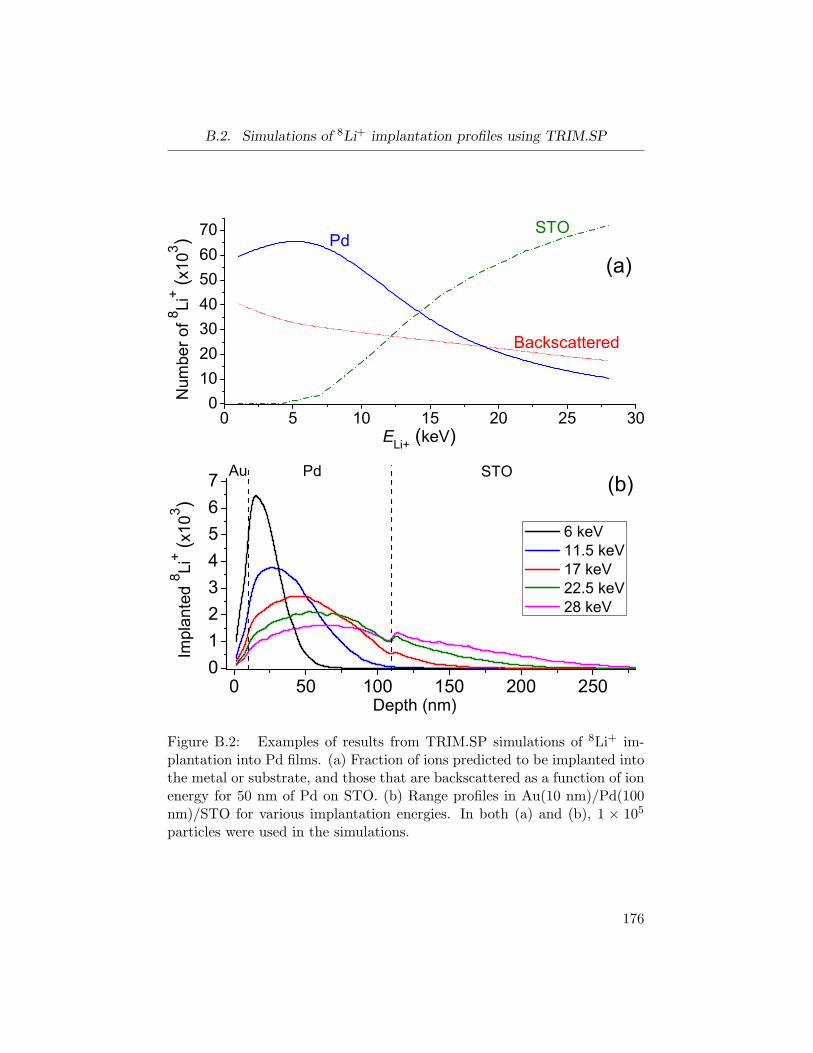
B.2. Simulations of 8Li+ implantation profiles using TRIM.SP
Figure B.2: Examples of results from TRIM.SP simulations of 8Li+ im-plantation into Pd films. (a) Fraction of ions predicted to be implanted intothe metal or substrate, and those that are backscattered as a function of ionenergy for 50 nm of Pd on STO. (b) Range profiles in Au(10 nm)/Pd(100nm)/STO for various implantation energies. In both (a) and (b), 1 × 10⁵
particles were used in the simulations.
176
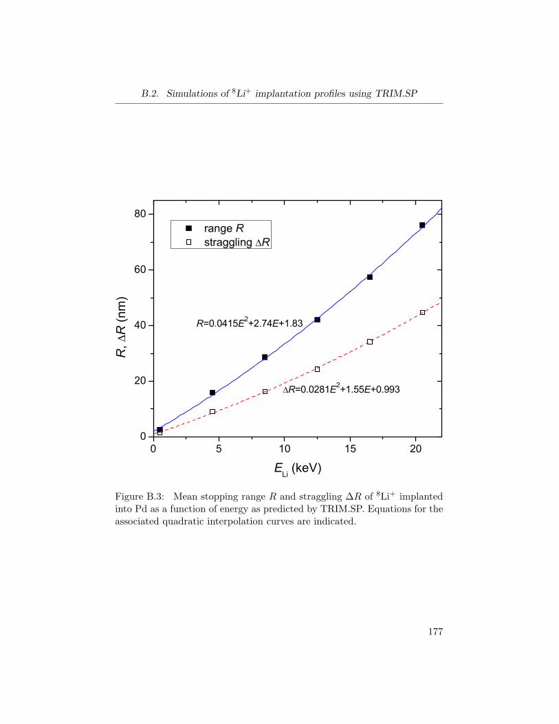
B.2. Simulations of 8Li+ implantation profiles using TRIM.SP
Figure B.3: Mean stopping range R and straggling ∆R of 8Li+ implantedinto Pd as a function of energy as predicted by TRIM.SP. Equations for theassociated quadratic interpolation curves are indicated.
177


![Probing the Relationship Between Detected Ion Intensity ... · as the power law function, I α Hm,whereI is the detected ion intensity,Hthefluence,and mthefittingparameter[3,4,6].At](https://static.fdocument.org/doc/165x107/5b4b10677f8b9a403d8ca20e/probing-the-relationship-between-detected-ion-intensity-as-the-power-law.jpg)