
UNIVERSIDAD COMPLUTENSE DE MADRIDm aster. Muchas gracias a J. Mariano L opez Castano~ por su ayuda...
256
UNIVERSIDAD COMPLUTENSE DE MADRID FACULTAD DE CIENCIAS FÍSICAS Departamento de Física Atómica, Molecular y Nuclear TESIS DOCTORAL Measurement of the neutrino mixing angle θ₁₃ in the Double Chooz experiment Medida del ángulo de mezcla de neutrinos θ₁₃ en el experimento Double Chooz MEMORIA PARA OPTAR AL GRADO DE DOCTOR PRESENTADA POR José Ignacio Crespo Anadón Directora Inés Gil Botella Madrid, 2016 © José Ignacio Crespo Anadón, 2015
Transcript of UNIVERSIDAD COMPLUTENSE DE MADRIDm aster. Muchas gracias a J. Mariano L opez Castano~ por su ayuda...
UNIVERSIDAD COMPLUTENSE DE MADRID
FACULTAD DE CIENCIAS FÍSICAS
Departamento de Física Atómica, Molecular y Nuclear
TESIS DOCTORAL
Measurement of the neutrino mixing angle θ₁₃ in the Double Chooz
experiment
Medida del ángulo de mezcla de neutrinos θ₁₃ en el experimento Double Chooz
MEMORIA PARA OPTAR AL GRADO DE DOCTOR
PRESENTADA POR
José Ignacio Crespo Anadón
Directora Inés Gil Botella
Madrid, 2016
© José Ignacio Crespo Anadón, 2015
Departamento de Fısica Atomica, Molecular y NuclearFacultad de Ciencias Fısicas
Measurement of the neutrinomixing angle θ13 in the
Double Chooz experiment
Medida del angulo de mezcla de neutrinos θ13
en el experimento Double Chooz
Tesis presentada por
Jose Ignacio Crespo Anadon
para optar al tıtulo de Doctor
Dirigida por
Dra. Ines Gil Botella
En Madrid, octubre de 2015


A mi familia.

Agradecimientos
En primer lugar quiero agradecer al CIEMAT, y en particular a Ines GilBotella, mi directora de tesis, el haberme dado la oportunidad de cumplir misueno de trabajar en Fısica de Partıculas. A Ines quiero agradecer especialmentesu constante apoyo a mi trabajo durante todos estos anos, y su apuesta por miformacion enviandome a reuniones de la colaboracion, conferencias, escuelas yestancias.
Quiero agradecer al “grupo de neutrinos” por haberme acogido. Gracias aCarmen Palomares por sus perspicaces observaciones sobre mis analisis y estatesis, y a Pau Novella por todo lo que he aprendido de el, tanto directamentecomo a traves del estudio de sus ejemplares programas. Tambien quiero agra-decer a Roberto Santorelli, que me enseno a dar mis primeros pasos en ROOT,y a Antonio Verdugo y Sergio Jimenez, por su ayuda en mi trabajo de fin demaster. Muchas gracias a J. Mariano Lopez Castano por su ayuda con los su-cesos accidentales y su explicacion de los sutilısimos factores de correccion. Sinsu magnıfico trabajo mis estudios de la eficiencia de deteccion de neutrones nohabrıan sido posibles. Y muchas gracias por hacer la convivencia siempre facilen todas las habitaciones que hemos compartido en reuniones y conferencias.Tengo una deuda de gratitud con Mariano y Diana Navas Nicolas por haberseencargado de los ultimos turnos de guardia para que yo pudiera centrarme enescribir la tesis.
Ha sido un privilegio compartir estos anos de Fısica con los miembros del de-partamento de Investigacion Basica en reuniones, seminarios y cafes cientıficos.Me siento muy afortunado de haber sido testigo de la emocion por el lanzamien-to del experimento AMS-02, el descubrimiento del boson de Higgs... He visitadomuchos lugares estos anos, pero hay algo que hace que trabajar en el CIEMATsea muy especial: la comunidad de becarios e ingenieros, personas inspiradoras;de todas ellas me llevo algo. Gracias por compartir la hora de la comida jun-tos y las conversaciones en la sobremesa. Y por los partidos de baloncesto, lasexcursiones, el cine, el Diplomacy, las cenas de Navidad y el amigo invisible...Atesoro grandes recuerdos de estos anos.
Hay unas personas que deben saber que esta tesis es tambien suya: mi familia.Esta tesis es un paso mas en mi vocacion cientıfica, que han apoyado regalando-me mis primeros libros sobre el espacio y la Fısica de Partıculas, trayendomeboletines de noticias cientıficas, revistas, acompanandome a conferencias... Mu-chas gracias por estar a mi lado y darme los medios para hacerla realidad. Latesis es la obra mas extensa que he escrito hasta ahora, y en una lengua que noes mi materna. Si ha sido posible es por ti, papa. Muchas gracias por ensenar-me la importancia del ingles desde muy pronto. Muchas gracias, mama, por tuayuda en los momentos mas duros de esta tesis de la mejor forma que podıas:
iii
iv
con comida (hecha con muchısimo amor). Estoy convencido de que esta tesis esmejor gracias a ti. Muchas gracias a mi hermano por ser un ejemplo de luchapara conseguir tus metas. Mi motivacion al escribir las partes sobre Fısica deneutrinos fue que algun dıa las leerıas. En el camino que ha llevado a esta tesishe aprendido muchas cosas, no solo de Fısica, y todo ha sido junto a ti, Sara.Muchas gracias por querer compartir tu vida conmigo, y por cosas mas munda-nas como ensenarme a conducir y practicamente regalarme un coche. Todo eltiempo ganado he podido invertirlo en mejorar mi trabajo, con una libertad dehorarios total que has soportado siempre con tu alegrıa. Muchas gracias por esasveces que te has encargado de todo lo demas para que yo me pudiera concentraren la tesis.
Para la realizacion de este trabajo he contado con una ayuda para personalinvestigador en formacion del Centro de Investigaciones Energeticas, Medioam-bientales y Tecnologicas; y financiacion de los programas FPA2010-15915 delMinisterio de Ciencia e Innovacion y FPA2013-40521 del Ministerio de Eco-nomıa y Competitividad. Asimismo, quiero agradecer las ayudas economicas delas organizaciones de la XXXIII Reunion Bienal de la Real Sociedad Espanolade Fısica en Santander (y el inmejorable alojamiento en el Palacio de la Mag-dalena), el XL International Meeting on Fundamental Physics en Benasque yla XXXIV Reunion Bienal de la Real Sociedad Espanola de Fısica en Valencia,que facilitaron mi asistencia a dichas conferencias.
Acknowledgements
The Double Chooz experiment is the result of a huge amount of work bymany people over many years. Although it is not possible to name them allhere, I have benefited so much from the good work that others did and theyhave my sincere gratitude.
During these years I had the pleasure to visit some of the institutions whichform the Double Chooz collaboration and learn personally from the physicistsin them.
I am thankful to the Double Chooz group at Nevis Laboratories for hostingme some weeks in June and July 2012. My understanding of the oscillationanalysis improved enormously there. And I felt privileged to live in the quaintNevis mansion.
I would like to thank Anatael Cabrera for inviting me to spend some weeks inNovember 2012 at the APC laboratory and sharing his scientific creativity andcontagious enthusiasm with me. Thanks also to Kazuhiro Terao for sharing hisknowledge on the neutron detection efficiency estimation for the first hydrogen-based analysis while at Paris.
I am deeply grateful to professors Masahiro Kuze and Masaki Ishitsuka,and to the Foreign Graduate Student Invitation Program of the Department ofPhysics of the Tokyo Institute of Technology for the opportunity to spend themonth of February 2013 there. The warm hospitality of them and the studentsYosuke Abe, Tomoyuki Konno, Ralitsa Sharankova made it an unforgettableexperience. The seeds of the new methods to estimate the neutron detectionefficiency were planted then. It was a pleasure to share this experience withJulia Haser.
I am thankful to Camillo Mariani, for hosting me again at Virginia Techin April 2013, and to Leonidas Kalousis for creating a welcoming atmosphere.Many thanks to Rachel Carr and Keith Crum for all the discussions about theoscillation analysis and for their superb documentation on the topic.
I am especially grateful to the “neutron detection efficiency working group”(Christian Buck, Anatael Cabrera, Antoine Collin, Zelimir Djurcic, Ines, JuliaHaser, Masaki Ishitsuka, Ralitsa Sharankova and Guang Yang). I had the priv-ilege to spend many hours in meetings with them, from which I learnt a lot ofphysics and improved my analyses as well.
Many thanks to the people at the chateau I had the pleasure to share adinner with during my on-site shifts. I am especially thankful to Didier Krynand Dave Reyna for making my first shift week (with the first off-off data) soenjoyable with their delicious food and card games.
v
vi
I want to acknowledge the financial support to attend the 37th InternationalConference on High Energy Physics (ICHEP 2014) in Valencia (Spain) and theInternational Neutrino Summer School (INSS 2014) in St. Andrews (Scotland)by the respective organizations.
Contents
List of Figures ix
List of Tables xv
Resumen 1
Abstract 5
Introduction 9
1 Neutrino physics 111.1 Neutrinos in the Standard Model . . . . . . . . . . . . . . . . . . 111.2 Neutrino oscillations . . . . . . . . . . . . . . . . . . . . . . . . . 14
1.2.1 Measurement of θ12 and ∆m221 . . . . . . . . . . . . . . . 18
1.2.2 Measurement of θ23 and |∆m232| . . . . . . . . . . . . . . 28
1.2.3 Measurement of θ13 . . . . . . . . . . . . . . . . . . . . . 311.3 Search for neutrino mass . . . . . . . . . . . . . . . . . . . . . . . 39
1.3.1 Kinematic limits . . . . . . . . . . . . . . . . . . . . . . . 391.3.2 Neutrinoless double beta decay . . . . . . . . . . . . . . . 401.3.3 Cosmology bounds . . . . . . . . . . . . . . . . . . . . . . 44
1.4 Open questions in neutrino oscillations . . . . . . . . . . . . . . . 45
2 The Double Chooz experiment 532.1 Experiment concept . . . . . . . . . . . . . . . . . . . . . . . . . 532.2 Electron antineutrino detection . . . . . . . . . . . . . . . . . . . 562.3 Detector design . . . . . . . . . . . . . . . . . . . . . . . . . . . . 59
2.3.1 Inner Detector . . . . . . . . . . . . . . . . . . . . . . . . 592.3.2 Outer Detector . . . . . . . . . . . . . . . . . . . . . . . . 612.3.3 Acquisition systems . . . . . . . . . . . . . . . . . . . . . 622.3.4 Calibration systems . . . . . . . . . . . . . . . . . . . . . 63
2.4 Signal simulation . . . . . . . . . . . . . . . . . . . . . . . . . . . 642.4.1 Antineutrino flux prediction . . . . . . . . . . . . . . . . . 652.4.2 Detector simulation . . . . . . . . . . . . . . . . . . . . . 71
3 Event reconstruction 753.1 Charge reconstruction . . . . . . . . . . . . . . . . . . . . . . . . 76
3.1.1 Improvement of single photoelectron efficiency . . . . . . 773.2 Photoelectron conversion . . . . . . . . . . . . . . . . . . . . . . . 803.3 Vertex reconstruction . . . . . . . . . . . . . . . . . . . . . . . . 83
vii
viii CONTENTS
3.4 Uniformity calibration . . . . . . . . . . . . . . . . . . . . . . . . 833.5 Energy conversion . . . . . . . . . . . . . . . . . . . . . . . . . . 843.6 Stability calibration . . . . . . . . . . . . . . . . . . . . . . . . . 863.7 Linearity calibration . . . . . . . . . . . . . . . . . . . . . . . . . 883.8 Energy scale in the Rate+Shape analysis . . . . . . . . . . . . . . 92
4 Antineutrino selections 954.1 Gadolinium selection . . . . . . . . . . . . . . . . . . . . . . . . . 95
4.1.1 Single trigger selection . . . . . . . . . . . . . . . . . . . . 974.1.2 Inverse beta-decay event selection . . . . . . . . . . . . . 994.1.3 Background vetoes and estimations . . . . . . . . . . . . . 104
4.2 Hydrogen selection . . . . . . . . . . . . . . . . . . . . . . . . . . 1194.2.1 Single trigger selection . . . . . . . . . . . . . . . . . . . . 1204.2.2 Inverse beta-decay event selection . . . . . . . . . . . . . 1214.2.3 Background vetoes and estimations . . . . . . . . . . . . . 129
5 Neutron detection efficiency 1455.1 Monte Carlo correction factor . . . . . . . . . . . . . . . . . . . . 1455.2 Neutron physics simulation . . . . . . . . . . . . . . . . . . . . . 1475.3 Neutron sources . . . . . . . . . . . . . . . . . . . . . . . . . . . . 149
5.3.1 Electron antineutrino source . . . . . . . . . . . . . . . . 1495.3.2 Californium-252 source . . . . . . . . . . . . . . . . . . . . 152
5.4 Neutron detection in the gadolinium selection . . . . . . . . . . . 1525.4.1 Gadolinium fraction . . . . . . . . . . . . . . . . . . . . . 1535.4.2 Neutron selection efficiency . . . . . . . . . . . . . . . . . 1565.4.3 Spill-in/out . . . . . . . . . . . . . . . . . . . . . . . . . . 1685.4.4 Summary . . . . . . . . . . . . . . . . . . . . . . . . . . . 169
5.5 Neutron detection in the hydrogen selection . . . . . . . . . . . . 1705.5.1 Hydrogen fraction . . . . . . . . . . . . . . . . . . . . . . 1705.5.2 Neutron selection efficiency . . . . . . . . . . . . . . . . . 1755.5.3 Spill . . . . . . . . . . . . . . . . . . . . . . . . . . . . . . 1795.5.4 Summary . . . . . . . . . . . . . . . . . . . . . . . . . . . 182
6 Oscillation analysis and measurement of θ13 1856.1 Reactor Rate Modulation analysis . . . . . . . . . . . . . . . . . 185
6.1.1 Gd results . . . . . . . . . . . . . . . . . . . . . . . . . . . 1896.1.2 H results . . . . . . . . . . . . . . . . . . . . . . . . . . . 1906.1.3 Combined Gd and H results . . . . . . . . . . . . . . . . . 195
6.2 Rate+Shape analysis . . . . . . . . . . . . . . . . . . . . . . . . . 2016.2.1 Gd results . . . . . . . . . . . . . . . . . . . . . . . . . . . 2046.2.2 H results . . . . . . . . . . . . . . . . . . . . . . . . . . . 2066.2.3 Spectral distortion . . . . . . . . . . . . . . . . . . . . . . 206
6.3 Two-detector outlook . . . . . . . . . . . . . . . . . . . . . . . . . 212
7 Conclusions 219
References 223
List of Figures
1.1 The two possible neutrino mass hierarchies. . . . . . . . . . . . . 191.2 Thermonuclear fusion reactions that produce neutrinos in the Sun. 201.3 Predicted energy spectra of the neutrino fluxes emitted by the Sun. 211.4 Solar neutrino flux measurements made by the SNO experiment. 251.5 Allowed regions on the tan2 θ12 −∆m2
21 plane from solar experi-ments, KamLAND and their combination. . . . . . . . . . . . . . 26
1.6 Solar electron neutrino survival probability as a function of theneutrino energy. . . . . . . . . . . . . . . . . . . . . . . . . . . . . 26
1.7 Ratio of the observed data in the KamLAND experiment to theno-oscillation prediction. . . . . . . . . . . . . . . . . . . . . . . . 27
1.8 Zenith angle distributions of the atmospheric neutrino candidatesobserved by Super-Kamiokande. . . . . . . . . . . . . . . . . . . . 30
1.9 The flavor composition of a 4 MeV reactor antineutrino flux as afunction of the distance to the reactor cores. . . . . . . . . . . . . 32
1.10 The CHOOZ detector. . . . . . . . . . . . . . . . . . . . . . . . . 341.11 Exclusion contours at 90% C.L. in the sin2(2θ13) −∆m2
31 planefrom the final analysis of the CHOOZ data. . . . . . . . . . . . . 35
1.12 Compilation of the first measurements of sin2(2θ13) by the reactorantineutrino experiments. . . . . . . . . . . . . . . . . . . . . . . 37
1.13 68% and 90% allowed regions on the sin2(2θ13) − δ plane fornormal hierarchy and inverted hierarchy. . . . . . . . . . . . . . . 38
1.14 The effective Majorana mass in neutrinoless double β decay as afunction of the lightest neutrino mass. . . . . . . . . . . . . . . . 43
1.15 Two-dimensional allowed regions from NuFit 2.0 to global datain 2014. . . . . . . . . . . . . . . . . . . . . . . . . . . . . . . . . 46
1.16 Allowed regions in the sin2(2θ)−∆m2 plane for MiniBooNE andLSND, and the upper limits from KARMEN and ICARUS ex-periments. . . . . . . . . . . . . . . . . . . . . . . . . . . . . . . . 50
2.1 Aerial view of the Double Chooz experimental site. . . . . . . . . 552.2 Top view layout of the experimental setups of the Double Chooz,
RENO and Daya Bay experiments. . . . . . . . . . . . . . . . . . 552.3 Feynman tree-level diagram for the inverse beta-decay reaction. . 562.4 Polynomial parametrization of the U-235 antineutrino spectrum,
inverse beta-decay cross-section and the detectable antineutrinospectrum. . . . . . . . . . . . . . . . . . . . . . . . . . . . . . . . 57
2.5 Double Chooz Far Detector schematic. . . . . . . . . . . . . . . . 60
ix
x LIST OF FIGURES
2.6 Block diagram of the readout and data acquisition systems in themain detector. . . . . . . . . . . . . . . . . . . . . . . . . . . . . 63
2.7 Sketch of the available deployment positions within the detectorusing the z axis and Guide Tube systems. . . . . . . . . . . . . . 65
2.8 Evolution of the fractional fission rates as a function of time cal-culated with the MURE code for a typical fuel cycle of a Choozreactor. . . . . . . . . . . . . . . . . . . . . . . . . . . . . . . . . 68
3.1 Example of a recorded digitized waveform from one readout chan-nel. . . . . . . . . . . . . . . . . . . . . . . . . . . . . . . . . . . . 76
3.2 Mean PMT multiplicity as a function of the reconstruction chargethreshold. Data from neutron captures on H using the Cf-252source. . . . . . . . . . . . . . . . . . . . . . . . . . . . . . . . . . 79
3.3 Fit to the energy spectrum of the Cf-252 neutrons captured on H. 803.4 Resolution of the neutron capture on H peak as a function of the
reconstruction charge threshold using the Cf-252 source. . . . . . 813.5 Gain as a function of the reconstructed charge for a typical read-
out channel. . . . . . . . . . . . . . . . . . . . . . . . . . . . . . . 823.6 Uniformity calibration maps made using neutrons captured on
hydrogen for the Gd selection. . . . . . . . . . . . . . . . . . . . . 853.7 Energy spectrum of the capture of neutrons on hydrogen from a
one-hour run taken with the Cf-252 source at the center of thedetector. . . . . . . . . . . . . . . . . . . . . . . . . . . . . . . . . 86
3.8 Ratio of the observed peak energy to the nominal energy as afunction of time after stability calibration for Po-212 and thecapture of spallation neutrons on H and on Gd. . . . . . . . . . . 87
3.9 Ratio of the peak visible energy in the DATA to that of theMC simulation after the application of the charge-non-linearitycorrection, plotted as a function of the average γ-ray energy, forcalibration sources at the center of the detector. . . . . . . . . . . 89
3.10 Energy resolution as a function of the peak visible energy forDATA and MC after the calibration. . . . . . . . . . . . . . . . . 91
4.1 Antineutrino selection flowchart. . . . . . . . . . . . . . . . . . . 964.2 Light noise and singles rates. . . . . . . . . . . . . . . . . . . . . 1004.3 Light noise cut variables: standard deviation of the PMTs charge
distribution versus standard deviation of the PMTs hit time dis-tribution for a DATA subsample. . . . . . . . . . . . . . . . . . . 100
4.4 Distribution of the light noise cut variable Qdiff for DATA. . . . 1014.5 Visible energy spectra of the triggers passing the muon veto be-
fore and after the light noise cuts are applied. . . . . . . . . . . . 1014.6 Delayed trigger visible energy spectra for IBD candidates in DATA
and MC in the gadolinium selection. . . . . . . . . . . . . . . . . 1024.7 Prompt-delayed trigger time interval for IBD candidates in DATA
and MC in the gadolinium selection. . . . . . . . . . . . . . . . . 1024.8 Prompt-delayed reconstructed vertices distance for IBD candi-
dates in DATA, MC and the off-time accidental sample withoutthe distance cut applied in the gadolinium selection. . . . . . . . 103
LIST OF FIGURES xi
4.9 Inner Veto PMT hit multiplicity and charge, Inner Detector-InnerVeto vertex distance and trigger time interval distributions usedin the definition of the IV veto. . . . . . . . . . . . . . . . . . . . 106
4.10 Correlation between the delayed trigger visible energy and theFV value before the FV veto is applied in the gadolinium selection.107
4.11 Delayed trigger reconstructed vertex distribution of IBD candi-dates before the FV veto is applied in the gadolinium selection. . 107
4.12 Prompt trigger energy, delayed trigger energy and prompt-delayedtrigger time interval distributions for the IBD candidates in thegadolinium selection before and after applying the backgroundvetoes, and for the rejected events by each veto. . . . . . . . . . . 108
4.13 Distribution of the highest 9Li/8He likelihood found for muon-prompt trigger pairs in the gadolinium selection. . . . . . . . . . 111
4.14 Prompt trigger energy spectrum of the 9Li/8He candidates mea-sured in the data. . . . . . . . . . . . . . . . . . . . . . . . . . . . 112
4.15 Lateral distance of the βn candidate prompt trigger vertex to themuon track. . . . . . . . . . . . . . . . . . . . . . . . . . . . . . . 112
4.16 Muon-prompt trigger time interval distribution used for the lowerlimit on the cosmogenic background rate in the gadolinium selec-tion. . . . . . . . . . . . . . . . . . . . . . . . . . . . . . . . . . . 113
4.17 Prompt trigger energy spectrum for the accidental background inthe gadolinium selection. . . . . . . . . . . . . . . . . . . . . . . . 117
4.18 Delayed trigger energy spectrum for the accidental backgroundin the gadolinium selection. . . . . . . . . . . . . . . . . . . . . . 117
4.19 Three-dimensional distribution of the input variables to the ANNclassifier: visible energy of the delayed trigger, time interval andthe reconstructed distance between the prompt and delayed trig-gers; for the IBD MC simulation and an accidental backgroundsample. . . . . . . . . . . . . . . . . . . . . . . . . . . . . . . . . 122
4.20 Distributions of the ANN input variables in the training samples. 1244.21 Artificial Neural Network classifier as a function of the input vari-
ables. . . . . . . . . . . . . . . . . . . . . . . . . . . . . . . . . . 1264.22 Distribution of the Artificial Neural Network classifier output. . . 1264.23 Distribution of the prompt-delayed reconstructed vertices dis-
tance in the hydrogen-based selection. . . . . . . . . . . . . . . . 1274.24 Delayed energy spectrum of the hydrogen-based selection. . . . . 1284.25 Distribution of the prompt-delayed trigger time interval in the
hydrogen-based selection. . . . . . . . . . . . . . . . . . . . . . . 1284.26 Prompt energy spectrum of the hydrogen-based selection before
the 1 MeV cut. . . . . . . . . . . . . . . . . . . . . . . . . . . . . 1294.27 Inner Detector-Inner Veto prompt and delayed trigger time in-
terval distributions. . . . . . . . . . . . . . . . . . . . . . . . . . . 1314.28 Correlation between the delayed trigger visible energy and the
FV value before the FV veto is applied in the hydrogen selection. 1324.29 Example of one PMT waveform showing 2 pulses within the flash-
ADC digitization window. . . . . . . . . . . . . . . . . . . . . . . 1334.30 Distribution of pulse start times from all Inner Detector PMTs
for a signal-like and a background-like prompt trigger. . . . . . . 134
xii LIST OF FIGURES
4.31 Distribution of pulse start times from all Inner Detector PMTsfor a prompt trigger with visible energy of 1.67 MeV which hasbeen tagged as ortho-positronium. . . . . . . . . . . . . . . . . . 135
4.32 Prompt energy spectrum of the IV-tagged events used to estimatethe shape of the fast neutron and stopping muon background inthe H selection. . . . . . . . . . . . . . . . . . . . . . . . . . . . . 137
4.33 Muon-prompt trigger time interval distribution used for the lowerlimit on the cosmogenic background rate in the hydrogen selection.139
4.34 Lateral distance of the cosmogenic βn candidate prompt triggervertex to the muon track in the hydrogen selection. . . . . . . . . 140
5.1 Neutron capture cross section as a function of the neutron kineticenergy for 157Gd, 155Gd, 1H and 12C. . . . . . . . . . . . . . . . 149
5.2 Intensities of the emitted γ ray energies in the radiative captureof a neutron by a Gd nucleus in Geant4 and NeutronTH. . . . . . 150
5.3 Energies and intensities of the emitted γ rays in the radiativecapture of a neutron by a 12C nucleus in Geant4 and NeutronTH. 150
5.4 Delayed energy spectra of the Californium-252 source used forthe measurement of the gadolinium fraction. . . . . . . . . . . . . 154
5.5 Deployment and reconstructed positions of the 252Cf source DATAduring the first calibration campaign. . . . . . . . . . . . . . . . . 155
5.6 Delayed energy spectra of the antineutrinos used for the measure-ment of the gadolinium fraction. . . . . . . . . . . . . . . . . . . 156
5.7 Inclusive neutron selection efficiency for the gadolinium analysisobtained with IBD neutrons. . . . . . . . . . . . . . . . . . . . . 158
5.8 Cumulative neutron selection efficiencies and correction factorsfor the gadolinium analysis as a function of the integrated volumeobtained with IBD neutrons. . . . . . . . . . . . . . . . . . . . . 161
5.9 Californium-252 source deployment positions during the secondcalibration campaign. . . . . . . . . . . . . . . . . . . . . . . . . 163
5.10 Neutron selection efficiencies for the Californium-252 source de-ployment positions along the Target axis during the second cali-bration campaign. . . . . . . . . . . . . . . . . . . . . . . . . . . 163
5.11 Reduction of the neutron selection efficiency as a function of thedistance to the Target center obtained from the antineutrino MCsimulation. . . . . . . . . . . . . . . . . . . . . . . . . . . . . . . 165
5.12 Neutron selection efficiency as a function of the distance to theTarget center obtained from the antineutrino DATA. . . . . . . . 166
5.13 Guide Tube californium-252 deployment positions used to com-pute the hydrogen fraction correction factor. . . . . . . . . . . . . 172
5.14 Delayed energy spectra of the Guide Tube californium-252 runsused to compute the Gamma Catcher hydrogen fraction. . . . . . 173
5.15 Delayed energy spectra of the IBD candidates reconstructed in-side the Gamma Catcher used to compute the hydrogen fraction. 174
5.16 Selected regions in the coincidence time-delayed energy plane bythe ANN cuts used in the neutron selection efficiency definition. . 177
5.17 Selected regions in the coincidence distance-delayed energy planeby the ANN cuts used in the neutron selection efficiency definition.177
5.18 Selected regions in the coincidence distance-time plane by theANN cuts used in the neutron selection efficiency definition. . . . 178
LIST OF FIGURES xiii
6.1 Daily rate of IBD candidates for the Gd-based and H-based νeselections since the beginning of data taking. . . . . . . . . . . . 188
6.2 Reactor Rate Modulation results for the Gd-based νe selection,treating the background rate as a free parameter. . . . . . . . . . 191
6.3 Reactor Rate Modulation results for the Gd-based νe selection,with the background rate constrained by its estimation. . . . . . 192
6.4 Reactor Rate Modulation results for the H-based νe selection,treating the background rate as a free parameter. . . . . . . . . . 193
6.5 Reactor Rate Modulation results for the H-based νe selection,with the background rate constrained by its estimation. . . . . . 194
6.6 Reactor Rate Modulation results for the combined Gd-based andH-based νe samples, treating the background rates as free param-eters. . . . . . . . . . . . . . . . . . . . . . . . . . . . . . . . . . . 197
6.7 Reactor Rate Modulation results for the combined Gd-based andH-based νe samples, with the background rates constrained bytheir estimations. . . . . . . . . . . . . . . . . . . . . . . . . . . . 199
6.8 Compilation of the measurements of sin2(2θ13) obtained with theReactor Rate Modulation analysis. . . . . . . . . . . . . . . . . . 200
6.9 Rate+Shape analysis results for the Gd-based νe selection. . . . 2056.10 Rate+Shape analysis results for the H-based νe selection. . . . . 2076.11 Prompt trigger visible energy spectrum in the vicinity of the dis-
tortion for the Gd sample, and the addition of the H-based sample.2096.12 Reactor Rate Modulation analysis applied to subsamples of the
Gd-based νe selection according to their prompt energy. . . . . . 2116.13 Expected precision of the Double Chooz Rate+Shape measure-
ment of sin2(2θ13) considering only IBD neutrons captured onGd, as a function of the elapsed time since the Far Detectorstarted the data taking. . . . . . . . . . . . . . . . . . . . . . . . 217
7.1 Summary of the most precise measurements of sin2(2θ13) by theDouble Chooz experiment. . . . . . . . . . . . . . . . . . . . . . . 220

xiv LIST OF FIGURES
List of Tables
1.1 Elementary fermion particles of the Standard Model. . . . . . . . 121.2 Left and right chirality projections of the elementary fermion
fields classified according to how they transform under the sym-metry group SU(3)C × SU(2)L ×U(1)Y. . . . . . . . . . . . . . . 13
1.3 Comparison between current reactor antineutrino experiments. . 341.4 Leading systematic uncertainties affecting the CHOOZ experi-
ment and their expectation in Double Chooz. . . . . . . . . . . . 351.5 Three-flavor neutrino oscillation parameters from NuFit 2.0 to
global data in 2014. . . . . . . . . . . . . . . . . . . . . . . . . . 47
2.1 Naturally occurring gadolinium isotopes. . . . . . . . . . . . . . . 582.2 Gamma-ray sources used for detector calibration. . . . . . . . . . 642.3 Mean energy released per fission of nuclide. . . . . . . . . . . . . 672.4 Reactor antineutrino flux normalization uncertainties. . . . . . . 712.5 Proton number, normalization correction and uncertainty for the
materials in which the antineutrinos interact. . . . . . . . . . . . 73
3.1 Best-fit values of the parameters of the parametrization of theenergy resolution. . . . . . . . . . . . . . . . . . . . . . . . . . . . 91
3.2 Summary of initialization values and uncertainties of the parame-ters of the visible energy of the MC simulation in the Rate+Shapefit. . . . . . . . . . . . . . . . . . . . . . . . . . . . . . . . . . . . 92
3.3 Initialization values and uncertainties of the coefficients of thequadratic polynomial which modelizes the visible energy of theMC simulation in the Rate+Shape fit for the two antineutrinoselections. . . . . . . . . . . . . . . . . . . . . . . . . . . . . . . . 93
4.1 Inefficiencies in the Gd-based νe selection due to the the background-oriented cuts and the associated correction factors to the normal-ization of the MC νe simulation. . . . . . . . . . . . . . . . . . . 97
4.2 Summary of the rates of the events passing the Gd-based νe se-lection. . . . . . . . . . . . . . . . . . . . . . . . . . . . . . . . . . 119
4.3 Inefficiencies in the H-based νe selection due to the the background-oriented cuts and the associated correction factors to the normal-ization of the MC νe simulation. . . . . . . . . . . . . . . . . . . 120
4.4 Summary of the rates of the events passing the H-based νe selection.143
xv
xvi LIST OF TABLES
5.1 Neutron selection efficiencies and correction factors for the gadolin-ium analysis computed with the νe source. . . . . . . . . . . . . . 159
5.2 Efficiency reduction factors along the axial and radial directionsof the Target volume computed with the νe source. . . . . . . . . 167
5.3 Compilation of the inputs and their uncertainties used to calcu-late the MC normalization correction factor due to the detectionefficiency for the Gd selection. . . . . . . . . . . . . . . . . . . . . 170
5.4 Neutron selection efficiencies and correction factors for the hy-drogen analysis computed with the νe source. . . . . . . . . . . . 180
5.5 Contributions to the νe normalization uncertainty of the H-basedselection due to the neutron migration between volumes. . . . . . 182
5.6 Compilation of the inputs and their uncertainties used to calcu-late the MC normalization correction factor due to the detectionefficiency for the H selection. . . . . . . . . . . . . . . . . . . . . 183
6.1 Comparison of the predicted and observed numbers of IBD can-didates in the Far Detector for the Gd-based and the H-based νeselections. . . . . . . . . . . . . . . . . . . . . . . . . . . . . . . . 186
6.2 Binning of the prompt trigger visible energy spectrum used inthe Rate+Shape analysis. . . . . . . . . . . . . . . . . . . . . . . 202
6.3 Normalization uncertainties relative to the signal prediction forthe Gd-based and H-based νe selections. . . . . . . . . . . . . . . 203
6.4 Input values and best-fit values, and their corresponding uncer-tainties, of the nuisance parameters of the Rate+Shape Gd analysis.204
6.5 Input values and best-fit values, and their corresponding uncer-tainties, of the nuisance parameters of the Rate+Shape H analysis.208
6.6 Summary of the background rates in the Gd-based νe selectionestimated in the Far Detector (FD) and the projected ones forthe Near Detector (ND). . . . . . . . . . . . . . . . . . . . . . . . 215
6.7 Summary of the estimated correlations between the Near and Fardetectors uncertainties. . . . . . . . . . . . . . . . . . . . . . . . . 216
Resumen
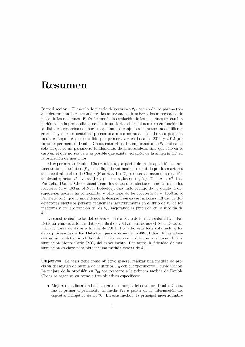
Introduccion El angulo de mezcla de neutrinos θ13 es uno de los parametrosque determinan la relacion entre los autoestados de sabor y los autoestados demasa de los neutrinos. El fenomeno de la oscilacion de los neutrinos (el cambioperiodico en la probabilidad de medir un cierto sabor del neutrino en funcion dela distancia recorrida) demuestra que ambos conjuntos de autoestados difierenentre sı, y que los neutrinos poseen una masa no nula. Debido a su pequenovalor, el angulo θ13 fue medido por primera vez en los anos 2011 y 2012 porvarios experimentos, Double Chooz entre ellos. La importancia de θ13 radica nosolo en que es un parametro fundamental de la naturaleza, sino que solo en elcaso en el que no sea cero es posible que exista violacion de la simetrıa CP enla oscilacion de neutrinos.
El experimento Double Chooz mide θ13 a partir de la desaparicion de an-tineutrinos electronicos (νe) en el flujo de antineutrinos emitido por los reactoresde la central nuclear de Chooz (Francia). Los νe se detectan usando la reaccionde desintegracion β inversa (IBD por sus siglas en ingles): νe + p → e+ + n.Para ello, Double Chooz cuenta con dos detectores identicos: uno cerca de losreactores (a ∼ 400 m, el Near Detector), que mide el flujo de νe donde la de-saparicion apenas ha comenzado, y otro lejos de los reactores (a ∼ 1050 m, elFar Detector), que lo mide donde la desaparicion es casi maxima. El uso de dosdetectores identicos permite reducir las incertidumbres en el flujo de νe de losreactores y en la deteccion de los νe, mejorando la precision en la medida deθ13.
La construccion de los detectores se ha realizado de forma escalonada: el FarDetector empezo a tomar datos en abril de 2011, mientras que el Near Detectorinicio la toma de datos a finales de 2014. Por ello, esta tesis solo incluye losdatos procesados del Far Detector, que corresponden a 489.51 dıas. En esta fasecon un unico detector, el flujo de νe esperado en el detector se obtiene de unasimulacion Monte Carlo (MC) del experimento. Por tanto, la fidelidad de estasimulacion es clave para obtener una medida exacta de θ13.
Objetivos La tesis tiene como objetivo general realizar una medida de pre-cision del angulo de mezcla de neutrinos θ13 con el experimento Double Chooz.La mejora de la precision en θ13 con respecto a la primera medida de DoubleChooz se organiza en torno a tres objetivos especıficos:
• Mejora de la linealidad de la escala de energıa del detector. Double Choozfue el primer experimento en medir θ13 a partir de la informacion delespectro energetico de los νe. En esta medida, la principal incertidumbre
1
2 RESUMEN
en la escala de energıa provenıa de la no-linealidad a baja energıa. Porello, reduciendo esta no-linealidad se reduce la incertidumbre en θ13.
• Estimacion de la eficiencia de deteccion de neutrones en el volumen del de-tector con nuevos metodos mas precisos. La incertidumbre en la eficienciade deteccion de los neutrones producidos en la reaccion νe+p→ e++n rep-resenta la mayor contribucion a la incertidumbre sistematica relacionadacon la deteccion de los νe. La estimacion precisa de esta eficiencia en losdatos reales y simulados, en todo el volumen del detector, es esencial paraminimizar la incertidumbre en la normalizacion de los antineutrinos, queafecta directamente a la incertidumbre en θ13.
• Ampliacion y desarrollo de la herramienta estadıstica para el analisis deoscilaciones en la fase con dos detectores. La herramienta para la medidade θ13 se desarrollo para la primera fase con el detector lejano unicamente.La inclusion del detector cercano permite realizar un analisis simultaneodel flujo de νe medido por los dos detectores, lo que representa la mejoracrucial en la precision de la medida de θ13 al producirse la cancelacion delas incertidumbres correlacionadas entre detectores.
Metodologıa El detector de Double Chooz es un calorımetro de centelladororganico lıquido dopado con gadolinio para facilitar la deteccion del neutron dela reaccion νe+p→ e+ +n. La interaccion de un νe en el detector se manifiestapor la coincidencia de dos senales, una que sigue inmediatamente a la interacciondel νe dada por la perdida de energıa cinetica del positron y su aniquilacion conun electron del detector (depositando una energıa en el rango 1−9 MeV), y otraque ocurre un tiempo despues debido a la captura radiativa del neutron en unnucleo. El tiempo entre senales y la energıa de la segunda senal dependen delnucleo que capture el neutron: ∼ 30µs para el Gd, que libera rayos γ con unaenergıa total de ∼ 8 MeV; y ∼ 200µs para el H, que libera un rayo γ de 2.2 MeV.La coincidencia de las dos senales permite discriminar la senal producida porlos sucesos de νe del ruido de fondo debido a otros procesos.
Se ha desarrollado una simulacion MC completa que predice el numero deνe en el detector. Esta simulacion incluye la emision de los νe en las desinte-graciones β− de los productos de fision en los reactores nucleares, que debe sermodelizada teniendo en cuenta las variaciones en la operacion de los reactoresy la evolucion del combustible nuclear, y la posterior interaccion de los νe en eldetector.
La colaboracion Double Chooz ha desarrollado dos selecciones de νe uti-lizando las capturas en Gd e H. La seleccion en Gd es la seleccion para la queoriginalmente se diseno el detector, y presenta la mejor relacion senal−ruido.Esta seleccion se ha optimizado respecto a aquella usada para los primeros re-sultados de θ13 de Double Chooz, aumentando la eficiencia de deteccion de νey reduciendo la contaminacion de fondos y las incertidumbres sistematicas. Laseleccion en H corresponde a un esfuerzo por obtener una medida de θ13 us-ando una muestra independiente y con mayor estadıstica. Debido a la bajaenergıa liberada en la captura del neutron, esta seleccion tiene una gran con-taminacion de coincidencias accidentales de la radiactividad ambiental. Unaestrategia basada en una red neuronal ha permitido reducir ampliamente estacontaminacion.
RESUMEN 3
Ambas selecciones de νe emplean asiduamente la energıa de los sucesos comocriterio de seleccion. Esta energıa se obtiene a partir de la recoleccion de la luzde centelleo por parte de tubos fotomultiplicadores, que la transforman en unpulso de corriente electrica que se digitaliza y posteriormente se reconstruye. Endicha reconstruccion se calibra la linealidad, la uniformidad y la estabilidad de larespuesta del detector. Para ello se usan fuentes de calibracion radioactivas quese introducen en el detector, la radiactividad natural y la inyeccion controladade luz dentro del detector.
La estimacion de la eficiencia de deteccion del neutron se realiza mediantedos fuentes: 252Cf y los neutrones producidos en la reaccion IBD. Esta eficienciaconsta de tres componentes: la fraccion de capturas de neutrones en el nucleoelegido respecto al total, la eficiencia de seleccion de capturas de neutrones enel detector, y el cambio en el numero de neutrones seleccionados por efectosde migracion de los neutrones en el detector. La eficiencia de seleccion debeestimarse en todo el volumen del detector: en el caso del 252Cf se obtiene a partirde la extrapolacion de medidas tomadas en zonas concretas del mismo; mientrasque los neutrones IBD, al estar distribuidos homogeneamente, proporcionan unamedida directa. Los efectos de migracion de neutrones se estiman comparandodistintas simulaciones MC.
La medida de θ13 usando solamente el Far Detector se obtiene de la com-paracion del numero de νe observados con el numero esperado dado por lasimulacion MC. Para mejorar la precision en θ13, la comparacion se realiza dedos formas: analizando la modulacion de la frecuencia de los sucesos de νe conla potencia de los reactores (analisis RRM por sus siglas en ingles), o analizandola forma y la normalizacion del espectro de positrones (analisis Rate+Shape).En la fase con dos detectores la medida de θ13 se obtiene fundamentalmente dela comparacion entre los datos del Near Detector con los del Far Detector. Paraello, es primordial determinar el grado de correlacion entre las incertidumbressistematicas de ambos detectores.
Resultados La reconstruccion de la energıa se ha mejorado a todos los niveles,obteniendo una respuesta mas lineal, homogenea y constante. En particular, laeficiencia de reconstruccion de senales de baja energıa ha aumentado un 4%. Losanalisis de la eficiencia de deteccion de neutrones han reducido la incertidumbrerelativa del 0.96% en la seleccion anterior en Gd a un 0.54% en la actual, y deun 1.25% en la seleccion anterior en H a un 0.42% en la actual. Ello, junto conlas mejoras en las selecciones de νe y el aumento en la cantidad de datos, hapermitido aumentar la precision de la medida de sin2(2θ13) mas de un 20% enel canal de Gd y mas de un 28% en el canal de H respecto a las medidas previasde Double Chooz.
El analisis RRM ha medido sin2(2θ13) = 0.090+0.034−0.035 en el canal de Gd, y
sin2(2θ13) = 0.095+0.038−0.039 en el canal de H. Al analizar simultaneamente ambos
canales se obtiene sin2(2θ13) = 0.088± 0.033.El analisis Rate+Shape ha medido sin2(2θ13) = 0.090+0.032
−0.029 en el canal deGd, y sin2(2θ13) = 0.124+0.030
−0.039 en el canal de H. Ademas se ha encontrado unadistorsion en el espectro de νe que sugiere la existencia de una nueva componenteen el espectro de los νe provenientes del reactor no tenida en cuenta por losmodelos del flujo actuales. No obstante, esta distorsion no afecta al valor deθ13, como demuestra el buen acuerdo con el resultado del analisis RRM.
4 RESUMEN
Gracias a las mejoras en la incertidumbre sistematica ya obtenidas y al usosimultaneo de los detectores cercano y lejano, se preve alcanzar una precisiondel 10 − 15% en sin2(2θ13) en el canal de Gd tras tres anos de toma de datoscon ambos detectores.
Conclusiones Los resultados presentados en esta tesis corresponden a las me-didas de θ13 mas precisas realizadas por el experimento Double Chooz hasta lafecha. Las mejoras en la escala de energıa, la seleccion de νe, y la estimacionde la eficiencia de deteccion de νe descritas en esta tesis demuestran la desta-cable precision alcanzable con un unico detector, y sientan la base sobre la queejecutar la medida con dos detectores. La medida con dos detectores mejorarasignificativamente la precision en θ13 debido a la supresion de las incertidum-bres sistematicas correlacionadas entre detectores, especialmente la del flujo delreactor que predomina sobre todas las demas.
Abstract
Introduction The neutrino mixing angle θ13 is one of the parameters thatrelate the neutrino flavor eigenstates to the mass eigenstates. The phenomenonof neutrino oscillations (the periodic change in the probability of measuring acertain neutrino flavor as a function of the distance traveled by the neutrino)proves that the flavor eigenstates are not aligned with the mass eigenstates, andthat neutrinos are massive particles. As a result of θ13 being a small angle,it was measured for the first time in 2011 and 2012 by several experiments,Double Chooz among them. The value of θ13 is important not only because itis a fundamental parameter of nature, but also because only if it is non-null CPviolation can occur in neutrino oscillations.
The Double Chooz experiment measures θ13 from the disappearance of elec-tron antineutrinos (νe) in the antineutrino flux emitted by the reactor cores ofthe Chooz nuclear power plant (France). The νe are detected using the inverseβ-decay reaction (IBD): νe + p → e+ + n. Two identical detectors are used:one close to the reactor cores (∼ 400 m, the Near Detector) which measures theνe flux where the disappearance has barely begun, and another away from thereactor cores (∼ 1050 m, the Far Detector) which measures the νe flux wherethe disappearance is almost maximal. As a consequence of the identicalnessbetween detectors, the uncertainties on the reactor νe flux and the detection ofthe νe are reduced, increasing the precision of the measurement of θ13.
The detectors were built in a phased approach: the Far Detector begun thedata taking in April 2011, and the Near Detector started the data taking bythe end of 2014. Hence, only the Far Detector data are covered in this thesis,totaling 489.51 run-days. In this one-detector phase, the expected νe flux in theFar Detector is obtained from a Monte Carlo (MC) simulation of the experiment.Therefore, the faithfulness of the simulation is crucial in order to measure θ13
accurately.
Objectives The general objective of the thesis is to provide a precision mea-surement of the neutrino mixing angle θ13 with the Double Chooz experiment.The improvement on the precision on θ13 with respect to the first Double Choozmeasurement is organized around three specific objectives:
• Improving the linearity of the energy scale of the detector. Double Choozwas the first experiment which measured θ13 using the energy spectrumof the νe. The main uncertainty on the energy scale of this measurementwas due to the energy scale non-linearity at low energy. Therefore, theuncertainty on θ13 can be brought down if the non-linearity is reduced.
5
6 ABSTRACT
• Precise estimation of the neutron detection efficiency in the detector vol-ume using new methods. The uncertainty on the detection of the neutronsproduced in the reaction νe+p→ e++n is the dominant systematic uncer-tainty on the detection of the νe. The precise estimation of the neutrondetection efficiency in the real and simulated data, in the full detectorvolume, is a fundamental step to minimize the uncertainty on the νe nor-malization, which affects directly the uncertainty on θ13.
• Expansion and development of the statistical tool for the oscillation anal-ysis in the two-detector phase. The statistical tool for measuring θ13 wasdeveloped for the first phase of the experiment, in which only the Far De-tector data is available. The addition of the Near Detector data allows tomeasure simultaneously the νe flux with the two detectors. This grants theexperiment the pivotal improvement on the precision of the measurementof θ13, since the correlated uncertainties between detectors are canceled.
Methods The Double Chooz detector is an organic liquid scintillator calorime-ter loaded with gadolinium to enhance the detection of the neutron from thereaction νe + p→ e+ + n. The interaction of one νe in the detector is revealedfrom the coincidence of two signals, a prompt one following the νe interactiongiven by the kinetic energy loss of the positron and its annihilation with anelectron from the detector (depositing an energy in the range 1 − 9 MeV), anda delayed one given by the radiative neutron capture on a nucleus. The timeinterval between signals and the energy of the second signal depend on the nu-cleus which captures the neutron: ∼ 30µs for Gd, which releases γ rays witha total energy of ∼ 8 MeV; and ∼ 200µs for H, which releases a single γ rayof 2.2 MeV. The coincidence of these two signals allows to discriminate the νeevents from other background events.
A full MC simulation of the experiment predicts the number of νe in thedetector. This simulation includes the emission of the νe in the β− decays of thefission products in the reactor cores, which must be modeled taking into accountthe variations due to the reactor operation and the nuclear fuel evolution, andthe νe interaction within the detector.
The Double Chooz collaboration has developed two νe selections using theneutron captures on Gd and on H. The Gd-based selection is the one for whichthe detector was originally designed, and features the best signal-to-backgroundratio. This selection has been optimized with respect to the one used in thefirst measurement of θ13 by Double Chooz, increasing the νe detection efficiencyand reducing the background contamination and the systematic uncertainties.The H-based selection is an endeavor to measure θ13 using an independent datasample with larger statistics. However, this selection has a sizable contaminationof accidental coincidences of the natural background radiation because of thelow energy released in the neutron capture. A selection strategy based on anartificial neural network has succeeded in reducing this contamination.
Both νe selections use the visible energy of the events as one of the mostimportant discriminating variables. The visible energy is obtained from thescintillation light collected by photomultiplier tubes, which transform it into anelectric current pulse which is digitized and then reconstructed offline. As apart of the reconstruction, the linearity, uniformity and stability of the detectorresponse are calibrated. In order to do so, radioactive sources deployed inside
ABSTRACT 7
of the detector, the natural radioactivity and controlled light injection in thedetector are used as calibration sources.
The neutron detection efficiency estimation is performed using two neutronsources: 252Cf and the neutrons produced in the IBD reaction. This efficiencyconsists of three components: the fraction of neutron captures in the chosennucleus with respect to the total neutron captures, the selection efficiency ofneutron captures within the detector, and the change in the number of selectedneutrons due to neutron migration effects in the detector. The selection effi-ciency must be evaluated in the full detector volume: in the case of 252Cf, itis inferred from the extrapolation of measurements at the source deploymentpositions; whereas the IBD neutrons produce a direct measurement since theyare homogeneously distributed. The neutron migration effects are estimatedfrom the comparison between MC simulations.
The measurement of θ13 using only the Far Detector is obtained from thecomparison of the number of νe observed to the one expected according to theMC simulation. In order to improve the precision on θ13, the comparison is madein two different ways: in the Reactor Rate Modulation (RRM) analysis, the νeinteraction rate is studied as a function of the reactor power; in the Rate+Shapeanalysis, the shape and the normalization of the positron spectrum are studied.In the two-detector phase, the measurement of θ13 is practically obtained fromthe comparison between the Near Detector data with the Far Detector data.Therefore, it is primordial to establish the degree of correlation between thesystematic uncertainties of both detectors.
Results The energy reconstruction has been improved in every aspect, achiev-ing a response more linear, homogeneous and constant. In particular, the ef-ficiency of the reconstruction of low energy signals has increased by 4%. Theanalyses of the neutron detection efficiency have reduced the relative uncer-tainty from 0.96% in the previous Gd-based selection to 0.54% in the currentone, and from 1.25% in the previous H-based selection to 0.42% in the currentone. These improvements together with the others in the νe selections and thedoubled statistics have made possible to increase the precision on sin2(2θ13) bymore than 20% in the Gd channel and more than 28% in the H channel withrespect to the previous measurements by Double Chooz.
The RRM analysis founds sin2(2θ13) = 0.090+0.034−0.035 in the Gd channel, and
sin2(2θ13) = 0.095+0.038−0.039 in the H channel. When the two channels are analyzed
simultaneously, the best fit is found at sin2(2θ13) = 0.088± 0.033.The Rate+Shape analysis founds sin2(2θ13) = 0.090+0.032
−0.029 in the Gd channel,and sin2(2θ13) = 0.124+0.030
−0.039 in the H channel. Moreover, a distortion in the νespectrum has been revealed, which suggests the existence of a new componentin the spectrum of the reactor νe which is not accounted for in the currentreactor-flux models. Nevertheless, this distortion does not affect the θ13 value,as it is demonstrated by the good agreement with the result from the RRManalysis.
As a consequence of the improvements on the systematic uncertainties al-ready obtained and the simultaneous use of the near and far detectors, a 10−15%precision on sin2(2θ13) in the Gd channel is expected after three years of datataking with both detectors.
8 ABSTRACT
Conclusions The results presented in this thesis correspond to the most pre-cise measurements of θ13 made by the Double Chooz experiment so far. Theimprovements on the energy scale, the νe selections, and the estimation of theνe detection efficiency described in this thesis demonstrate the remarkable pre-cision which has been achieved with only one detector, and pave the way tomeasure θ13 with two detectors. The measurement of θ13 in the two-detectorphase will improve significantly the precision on θ13 since the systematic uncer-tainties correlated between detectors are suppressed, especially the one on thereactor flux, which prevails over all the others.
Introduction
Since the beginning of philosophy, the αρχη, the ultimate substance of na-ture, has been a central question in our attempt to understand rationally thereality. Nowadays, the most precise answer to that question is given by theStandard Model of Elementary Particle Physics. The Standard Model has beenable to explain and predict phenomena in agreement with experimental mea-surements to an amazing precision. However, it is an incomplete theory sinceit does not include gravity. Moreover, the recent astrophysical and cosmologi-cal observations require the existence of two mysterious agents known as darkmatter and dark energy, for which the Standard Model offers no explanation.In addition, the Standard Model requires a relatively large number of inputparameters which must be determined exclusively by experiments. This has ledthe Standard Model to be regarded as an effective theory of nature, with newphysics awaiting to be discovered at higher energies.
So there is the incontestable success of the Standard Model over many yearsof experimental tests, and there is the conviction that there is physics beyondit; and in between, the neutrinos. As it will be explained in chapter 1, neutrinoswere included in the Standard Model as massless particles from the availabledata when the theory was developed. However, the observed phenomenon ofneutrino oscillations, in which the different types (flavors) of neutrinos trans-mute into each other periodically, requires them to be massive and mix amongthemselves; so that the original Standard Model implementation must be modi-fied. Even though the Standard Model is able to give masses to neutrinos in thesame way it gives masses to the other elementary particles, the fact that neutrinomasses are much smaller than the others suggests that a different mechanismmight be behind them. In any case, in order to describe the neutrino oscilla-tions, the number of fundamental parameters of the Standard Model must beenlarged. The neutrino mixing angle θ13 is one of these new parameters. Whatmakes θ13 special is that, unlike the other two neutrino mixing angles θ12 andθ23, it has been measured to be relatively small. In fact, when the researchthat has led to this thesis started, only an upper limit on its value had beenestablished. The measurement of θ13 is important not only because it is a funda-mental parameter of nature, but also because only if it is non-null CP violationcan take place in neutrino oscillations in vacuum, which might be related to theprevalence of matter over antimatter in our Universe, one of the observationsfor which the Standard Model does not provide a satisfactory answer.
The Double Chooz experiment, introduced in chapter 2, was designed tomeasure θ13 using the electron antineutrinos (νe) emitted from the two reactorcores of the Chooz nuclear power plant in France. For distances of the orderof a kilometer, the fraction of νe which oscillate into undetectable flavors is
9
10 INTRODUCTION
proportional to sin2(2θ13). In order to measure the disappearance of νe, twodetectors are used: the Near Detector at ∼ 400 m from the reactors, where theoscillation is almost undeveloped, and the Far Detector at ∼ 1050 m, where theoscillation is sizable. The νe are detected via the inverse-β decay reaction (IBD),νe + p→ e+ + n, in a liquid scintillator calorimeter loaded with gadolinium toenhance the detection of the neutron captures. The experiment followed a stagedapproach: the Far Detector started the data taking first in April 2011, and theNear Detector joined the data taking in December 2014. Only the Far Detectordata are covered in this thesis. In order to be able to measure θ13 preciselyduring the single-detector phase of the experiment, a detailed simulation topredict the number of νe in the detector was developed.
Chapter 3 describes the event reconstruction in Double Chooz. A specialemphasis is put on the energy reconstruction, since this variable plays a fun-damental role in the selection of the νe events and the measurement of θ13.In addition, the improvement of the linearity at low energies is reviewed, sincethis was one of my first contributions to the Double Chooz measurement of θ13
published in 2012 [1].The selection of νe events is explained in detail in chapter 4. The Double
Chooz collaboration has developed two selections depending on whether the IBDneutron is captured on a gadolinium or a hydrogen nucleus. In this chapter theestimation of the different backgrounds contaminating the selected samples isdescribed too.
Chapter 5 reviews the estimation of the neutron detection efficiency in theexperimental data and the Monte Carlo simulations. The neutron detection isthe dominant component of the νe detection systematic uncertainty for the Gd-based selection, and the next-to-leading uncertainty for the H-based selection.Therefore, a precise estimation is mandatory, since it conditionates the precisionon the measurement of θ13. The estimations using the IBD neutrons representmy central contributions to the Double Chooz measurements of θ13 in the Gdchannel, published in 2014 [2], and in the H channel, which is about to besubmitted for publication.
The two statistical analyses used to extract the value of θ13 from the dataare described in chapter 6. It also includes the projected sensitivity of DoubleChooz once the data from both Near and Far Detectors is analyzed, using theextension to two detectors of the statistical analysis which I contributed todevelop.
In chapter 7 the conclusions of this work are presented.Finally, some conventions used throughout this thesis:
• Natural units (~ = c = 1) are used unless stated otherwise.
• When the differentiation between actual data taken whith detector and thecorresponding one obtained from the Monte Carlo simulation is important,the capitalized DATA and MC are used, respectively.
• The term “neutrino(s)” is used sometimes to denote both neutrino(s) andantineutrino(s) when the distinction is not relevant or both apply.
• Uncertainties are given at 68% C.L. unless noted otherwise.
Chapter 1
Neutrino physics
This chapter is an overview of the basics of neutrino physics in order to con-textualize the measurement of the θ13 parameter pursued by the Double Choozexperiment. In section 1.1 neutrinos are introduced in the theoretical frame-work of the Standard Model. Section 1.2 discusses the phenomenon of neutrinoflavor oscillations, a consequence of the neutrinos being massive particles whichmix between themselves. In this section, the experimental determination of theparameters which drive the oscillations is also reviewed. Section 1.3 describesthe different methods being used in order to measure the mass of the neutrinos.Finally, section 1.4 lists the most important questions in neutrino oscillationsyet to be answered.
1.1 Neutrinos in the Standard Model
The Standard Model is a renormalizable relativistic quantum field theorydefined by the local gauge symmetry SU(3)C × SU(2)L × U(1)Y (see [3] foran introduction). The symmetry group SU(3)C, where the subscript C de-notes the color charge, determines the interaction between color-charged fields,known also as the strong interaction, which is described by the theory of quan-tum chromodynamics (QCD). The strong interaction is mediated by 8 masslessbosons, the gluons, with JP = 1−, where J is the spin in natural units andP is the parity. The symmetry group SU(2)L × U(1)Y, where L denotes theweak isospin of the left-handed fields and Y the weak hypercharge, describesthe dynamics of the electroweak interaction [4, 5, 6]. The electroweak symmetrySU(2)L×U(1)Y is spontaneously broken through the so-called Higgs mechanism[7, 8, 9] into U(1)EM, the symmetry group of the electromagnetic interaction,described by the theory of quantum electrodynamics (QED). The electroweaksymmetry breaking results in the intermediate vector bosons (JP = 1−) of theweak interaction, W+, W−, Z, acquiring mass (mW± = 80.385 ± 0.015 GeV,mZ = 91.1876 ± 0.0021 GeV [10]); while the photon, γ, the mediator of theelectromagnetic interaction, remains massless. Evidence of the breaking mech-anism has been found recently in the form of the predicted Higgs scalar boson(JP = 0+), discovered with a mass of 125.7± 0.4 GeV [10] by the ATLAS andCMS experiments at the LHC at CERN [11, 12].
The fermion fields (J = 1/2) are not predicted by the mathematical structure
11
12 CHAPTER 1. NEUTRINO PHYSICS
QGeneration
1st 2nd 3rd
+ 23
u c t
Quarks( 2.3+0.7−0.5 MeV ) ( 1275 ± 25MeV ) ( 173.21 ± 0.51 ± 0.71GeV )
− 13
d s b( 4.8+0.5
−0.3 MeV ) ( 95 ± 5MeV ) ( 4.18 ± 0.03GeV )
0 νe νµ ντ
Leptons( < 2 eV ) ( < 0.19MeV ) ( < 18.2MeV )
−1 e µ τ( 0.511MeV ) ( 105.658MeV ) ( 1776.82 ± 0.16MeV )
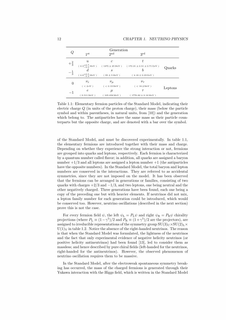
Table 1.1: Elementary fermion particles of the Standard Model, indicating theirelectric charge Q (in units of the proton charge), their mass (below the particlesymbol and within parentheses, in natural units, from [10]) and the generationwhich belong to. The antiparticles have the same mass as their particle coun-terparts but the opposite charge, and are denoted with a bar over the symbol.
of the Standard Model, and must be discovered experimentally. In table 1.1,the elementary fermions are introduced together with their mass and charge.Depending on whether they experience the strong interaction or not, fermionsare grouped into quarks and leptons, respectively. Each fermion is characterizedby a quantum number called flavor; in addition, all quarks are assigned a baryonnumber +1/3 and all leptons are assigned a lepton number +1 (the antiparticleshave the opposite numbers). In the Standard Model, the total baryon and leptonnumbers are conserved in the interactions. They are referred to as accidentalsymmetries, since they are not imposed on the model. It has been observedthat the fermions can be arranged in generations or families, consisting of twoquarks with charges +2/3 and −1/3, and two leptons, one being neutral and theother negatively charged. Three generations have been found, each one being acopy of the preceding one but with heavier elements. If neutrinos did not mix,a lepton family number for each generation could be introduced, which wouldbe conserved too. However, neutrino oscillations (described in the next section)prove this is not the case.
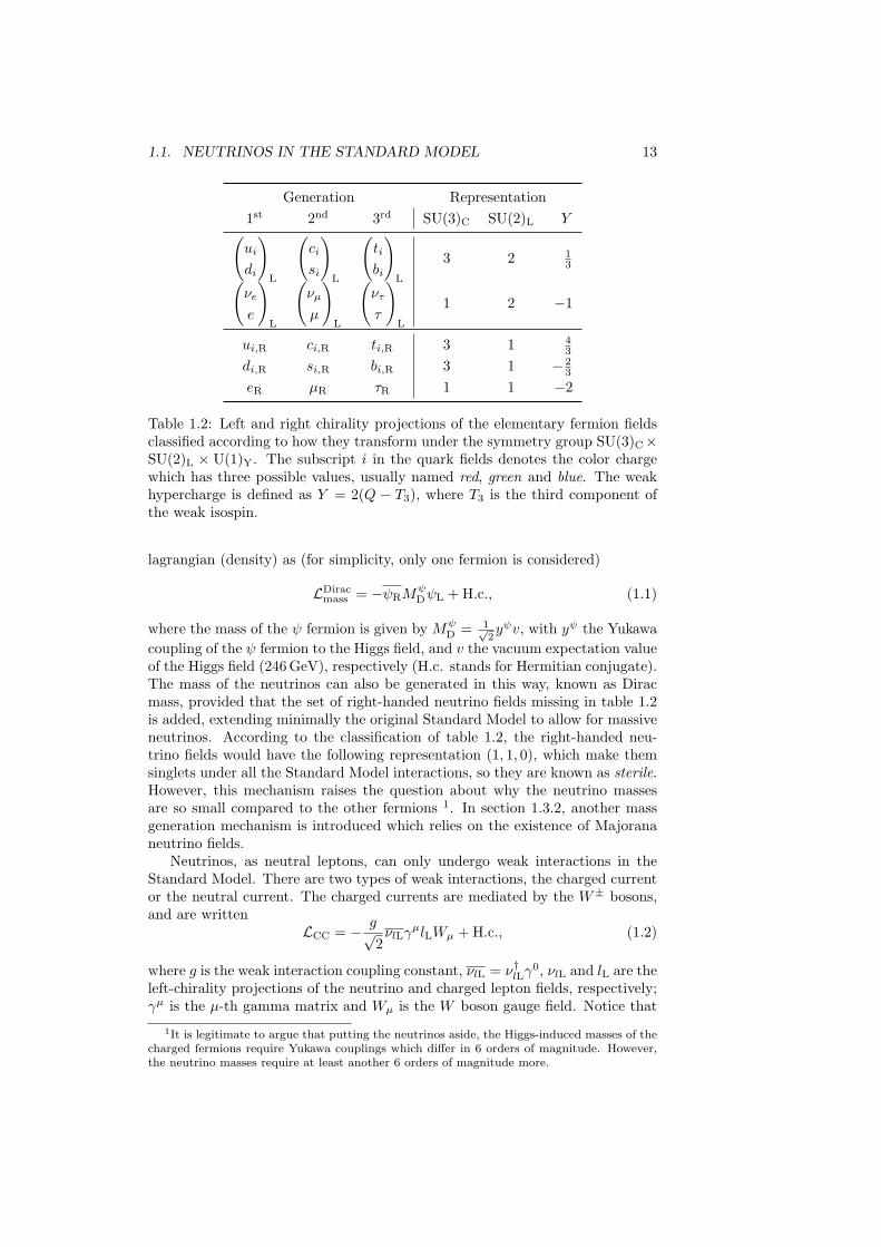
For every fermion field ψ, the left ψL = PLψ and right ψR = PRψ chiralityprojections (where PL ≡ (1−γ5)/2 and PR ≡ (1+γ5)/2 are the projectors), areassigned to irreducible representations of the symmetry group SU(3)C×SU(2)L×U(1)Y in table 1.2. Notice the absence of the right-handed neutrinos. The reasonis that when the Standard Model was formulated, the lightness of the neutrinosand the fact that only experimental evidence of negative helicity neutrinos (orpositive helicity antineutrinos) had been found [13], led to consider them asmassless; and hence described by pure chiral fields (left-handed for the neutrinos,right-handed for the antineutrinos). However, the observed phenomenon ofneutrino oscillation requires them to be massive.
In the Standard Model, after the electroweak spontaneous symmetry break-ing has occurred, the mass of the charged fermions is generated through theirYukawa interaction with the Higgs field, which is written in the Standard Model
1.1. NEUTRINOS IN THE STANDARD MODEL 13
Generation Representation1st 2nd 3rd SU(3)C SU(2)L Y(ui
di
)L
(ci
si
)L
(ti
bi
)L
3 2 13(
νe
e
)L
(νµ
µ
)L
(ντ
τ
)L
1 2 −1
ui,R ci,R ti,R 3 1 43
di,R si,R bi,R 3 1 − 23
eR µR τR 1 1 −2
Table 1.2: Left and right chirality projections of the elementary fermion fieldsclassified according to how they transform under the symmetry group SU(3)C×SU(2)L × U(1)Y. The subscript i in the quark fields denotes the color chargewhich has three possible values, usually named red, green and blue. The weakhypercharge is defined as Y = 2(Q − T3), where T3 is the third component ofthe weak isospin.
lagrangian (density) as (for simplicity, only one fermion is considered)
LDiracmass = −ψRM
ψDψL + H.c., (1.1)
where the mass of the ψ fermion is given by MψD = 1√
2yψv, with yψ the Yukawa
coupling of the ψ fermion to the Higgs field, and v the vacuum expectation valueof the Higgs field (246 GeV), respectively (H.c. stands for Hermitian conjugate).The mass of the neutrinos can also be generated in this way, known as Diracmass, provided that the set of right-handed neutrino fields missing in table 1.2is added, extending minimally the original Standard Model to allow for massiveneutrinos. According to the classification of table 1.2, the right-handed neu-trino fields would have the following representation (1, 1, 0), which make themsinglets under all the Standard Model interactions, so they are known as sterile.However, this mechanism raises the question about why the neutrino massesare so small compared to the other fermions 1. In section 1.3.2, another massgeneration mechanism is introduced which relies on the existence of Majorananeutrino fields.
Neutrinos, as neutral leptons, can only undergo weak interactions in theStandard Model. There are two types of weak interactions, the charged currentor the neutral current. The charged currents are mediated by the W± bosons,and are written
LCC = − g√2νlLγ
µlLWµ + H.c., (1.2)
where g is the weak interaction coupling constant, νlL = ν†lLγ0, νlL and lL are the
left-chirality projections of the neutrino and charged lepton fields, respectively;γµ is the µ-th gamma matrix and Wµ is the W boson gauge field. Notice that
1It is legitimate to argue that putting the neutrinos aside, the Higgs-induced masses of thecharged fermions require Yukawa couplings which differ in 6 orders of magnitude. However,the neutrino masses require at least another 6 orders of magnitude more.
14 CHAPTER 1. NEUTRINO PHYSICS
the flavor of the neutrino νl, with l = e, µ, τ , is assigned according to the chargedlepton l which accompanies it in the charged current interaction.
Neutral currents are mediated by the Z boson, and are written
LNC = − g
2 cos θWνlLγ
µνlLZµ, (1.3)
where θW is the weak mixing angle parameter, and Zµ is the Z boson gaugefield.
The existence of the (electron) neutrino was first postulated by Pauli in 1930[14]. According to Pauli, in order to explain the integer spin of nuclei 14N and6Li, and at the same time the apparent non-conservation of energy in the β de-cay; a light neutral fermion with spin 1/2 existed within the nucleus, which wasemitted along the electron in the β decay. Pauli’s proposal turned out to be twodifferent particles, the neutron, discovered by Chadwick in 1932 [15]; and theneutrino, “little neutral one” in Italian, named by Fermi, who formulated thefirst theory of β decay [16], which included this new particle. The discovery ofthe neutrino (to be precise, the electron antineutrino) was made by Reines andCowan in 1956, when they detected the electron antineutrinos emitted by theSavannah River nuclear reactor [17]. The existence of a second neutrino flavordifferent from the electron one, the muon neutrino, was hypothesized to explainthe muon decay modes [18, 19]. It was found in 1962 by Lederman, Schwartz,Steinberger et al. in an experiment at Brookhaven National Laboratory usinga neutrino beam produced by the decay in flight of pions [20]. The tau neu-trino was not directly observed until the year 2000 by the DONUT experimentat Fermi National Accelerator Laboratory [21]. However, given the recurrentneutrino-charged lepton symmetry, its existence could be anticipated since thediscovery of the tau lepton in 1975 by Perl et al. at the SPEAR e+e- collider atSLAC [22]. Moreover, the three-flavor neutrino paradigm was firmly establishedsince the analysis of the decay width of the Z boson by the ALEPH, DELPHI,L3 and OPAL detectors at LEP at CERN, which determined from the invisiblepartial width that the number of neutrinos 2 is 2.9840± 0.0082 [23].
1.2 Neutrino oscillations
In the three-flavor framework of massive neutrinos, the relationship betweenthe neutrino flavor eigenstates that participate in the weak interaction, |νl〉,with l = e, µ, τ , and the mass eigenstates, |νj〉, which describe the propagationin vacuum can be written
|νl〉 =3∑j=1
U∗lj |νj〉 , (1.4)
where the sum in j is over the three mass eigenstates with mass mj . U is a3 × 3 unitary matrix which will be non-diagonal if neutrinos mix, playing anequivalent role to the CKM (Cabibbo-Kobayashi-Maskawa) matrix in the quarksector [24, 25]. U is known as the Pontecorvo-Maki-Nakagawa-Sakata matrix,or PMNS for short [26, 27, 28].
2Specifically, the number of light neutrinos (mν < mZ/2) which experience weak interac-tions, also known as active neutrinos.
1.2. NEUTRINO OSCILLATIONS 15
Among the 9 parameters that define a 3 × 3 unitary matrix like U , 5 (3)phases can be absorbed in the redefinition of the neutrino fields if they areDirac (Majorana), so only 4 (6) remain as independent. The flavor and masseigenstates can be regarded as two bases of a vector space of dimension 3, soU would be the matrix to change of basis. Therefore, U can be parametrizedin terms of three Euler angles, θ12, θ23 and θ13, known as the neutrino mixingangles. In the case of Dirac neutrinos, the remaining parameter is a CP-violatingphase, δ, and the most general parametrization of U is:
U =
1 0 00 c23 s23
0 −s23 c23
c13 0 s13e−iδ
0 1 0−s13eiδ 0 c13
c12 s12 0−s12 c12 0
0 0 1
=
c12c13 s12c13 s13e−iδ
−s12c23 − c12s23s13eiδ c12c23 − s12s23s13eiδ s23c13
s12s23 − c12c23s13eiδ −c12s23 − s12c23s13eiδ c23c13
(1.5)
where cij ≡ cos(θij), sij ≡ sin(θij), with θij ∈ [0, π/2] and δ ∈ (−π, π]. In thecase of Majorana neutrinos, two additional CP-violating phases, α1 and α2 areneeded; so U must be multiplied by1 0 0
0 eiα1 00 0 eiα2
(1.6)
However, these two phases do not affect the neutrino oscillations as we will see.Let |νl(t)〉 be a neutrino after a time t, which originally was created with
flavor l, |νl(t = 0)〉 = |νl〉. According to equation 1.4, it can be expressed as
|νl(t)〉 =3∑j=1
U∗lj |νj(t)〉 , (1.7)
where |νj(t)〉 is the time-evolution of the mass eigenstate |νj〉. Following [29],we describe the mass eigenstate as a plane wave 3; its time-evolution is givenby the Scrodinger equation:
iddt|νj(t)〉 = Ej |νj〉 , (1.8)
where Ej =√|~pj |2 +m2
j . Therefore, equation 1.7 is written as
|νl(t)〉 =3∑j=1
U∗lje−iEjt |νj〉 . (1.9)
If the mass eigenstate |νj〉 is expressed as a sum of the flavor eigenstates byinverting equation 1.4,
|νl(t)〉 =∑
l′=e,µ,τ
3∑j=1
U∗lje−iEjtUl′j
|νl′〉 , (1.10)
3More sophisticated descriptions based on wave packets (e.g. [30]) or quantum field theory(e.g. [31]) arrive at the same neutrino oscillation probability, but the plane wave is instructivebecause of its simplicity.
16 CHAPTER 1. NEUTRINO PHYSICS
which shows that after a time t, |νl(t)〉 is found in a superposition of flavor eigen-states, with coefficients given by the factor within parentheses. The probabilityto detect a particular flavor l′, Pll′ , is given by
Pll′(t) =∣∣ 〈νl′ | νl(t)〉 ∣∣2 =
3∑j,k=1
U∗ljUl′jUlkU∗l′ke−i(Ej−Ek)t. (1.11)
Since all experiments made so far use ultrarelativistic neutrinos, the energyof the mass eigenstate |νj〉 can be approximated by
Ej ' E +m2j
2E, (1.12)
with E ' |~pj | the neutrino energy neglecting the mass contribution. Then,
Ej − Ek '∆m2
jk
2E, (1.13)
where∆m2
jk ≡ m2j −m2
k. (1.14)
Moreover, in the experiments the production time of the neutrino is not known(at least with enough precision), but the distance L between the source and thedetector can be measured precisely. For ultrarelativistic neutrinos, t ' L; sothe probability of equation 1.11 becomes
Pll′(L,E) =3∑
j,k=1
U∗ljUl′jUlkU∗l′k exp
(−i
∆m2jkL
2E
). (1.15)
Because e−ix = cosx − i sinx, the probability of detecting a neutrino offlavor l′ oscillates as a function of the distance traveled L or the neutrino en-ergy E, hence the name neutrino oscillations. For a fixed L/E, the oscillationfrequency is determined by ∆m2
jk. Therefore, the observation of neutrino oscilla-tion implies that ∆m2
jk 6= 0, that is, neutrinos are massive and non-degenerated(mj 6= mk). The amplitude of the oscillations depends on the magnitude of theU matrix elements; however, it can be shown that in the product U∗ljUl′jUlkU
∗l′k,
the Majorana phases of equation 1.6 cancel out, so the oscillation amplitude isonly a function of the three mixing angles, θ12, θ23, θ13, and the CP-violatingphase δ.
The neutrino oscillation experiments are designed so that L and E can beknown (within uncertainties); so the unknown physical parameters (mixing an-gles, squared-mass differences, CP-violating phase) can be inferred from themeasurement of the probability of detecting a flavor l′ in a neutrino flux createdwith a flavor l. If l = l′, the probability is called survival probability ; if l 6= l′, itis called transition probability.
So far, only neutrinos have been considered. The derivation for antineutrinosfollows along the sames lines of the neutrino case, except that the coefficientsof the antineutrino mass eigenstates in an expression analogous to equation 1.4are the complex conjugate of the neutrino ones. Consequently, it is useful to
1.2. NEUTRINO OSCILLATIONS 17
rewrite the oscillation probability in equation 1.15 as
Pll′(L,E) = δll′ − 4∑j>k
Re(U∗ljUl′jUlkU
∗l′k
)sin2
(∆m2
jkL
4E
)
± 2∑j>k
Im(U∗ljUl′jUlkU
∗l′k
)sin
(∆m2
jkL
2E
),
(1.16)
where the sign of the imaginary part is + for neutrinos and − for antineutrinos.Hence, the CP violation will be determined by magnitude of the imaginary part.Furthermore, since CPT symmetry requires the probabilities P (νl → νl) andP (νl → νl) to be equal, CP violation effects will appear only in the transitionprobabilities.
Under certain circumstances, such as when there are two squared-massdifferences, ∆m2
jk and ∆m2ik with i 6= j, which differ greatly in magnitude,
∆m2jk >> ∆m2
ik, so that is possible to find a L/E range in which one oscilla-tion has developed (∆m2
jk ∼ 1) while the other not, the three-neutrino mixingcan be approximated by a two-flavor mixing. A two-flavor approximation canalso be used if one of the mixing angles is much smaller than the others; or ifthe detector is only sensitive to one flavor l, so the other two flavors can be com-bined in an effective indistinguishable flavor x (e.g. if the detector only “sees”νe, the effective flavor νx = ε νµ +
√1− ε2 ντ can be defined, with ε ∈ [0, 1]).
In this case, the relationship between flavor eigenstates and mass eigenstates isreduced to (
|νl〉|νx〉
)=(
cos θ sin θ− sin θ cos θ
)(|ν1〉|ν2〉
), (1.17)
where only one mixing angle θ exists. Defining the unique squared-mass differ-ence
∆m2 ≡ m22 −m2
1, (1.18)
where m1 is taken as the lightest mass, so ∆m2 > 0; the transition probabilityreads
P 2νlx (l 6=x)(L,E) = sin2(2θ) sin2
(∆m2L
4E
), (1.19)
and the survival probability
P 2νll (L,E) = 1− Plx (l 6=x)(L,E). (1.20)
The oscillation probabilities just derived apply to the case in which the neu-trinos propagate in vacuum. If the neutrinos traverse a medium dense enoughso that matter effects become important, the propagation is affected by thecoherent forward elastic scattering with the particles composing medium [32].For electron neutrinos and antineutrinos, the charged current weak interactionwith a homogeneous gas of unpolarized electrons (
(−)ν e e
− CC−−→ (−)ν e e
−) induces apotential
VCC = ±√
2GFNe, (1.21)
where the sign is + for νe (− for νe), GF =√
2 g2
8m2W
is the Fermi couplingconstant, and Ne is the electron density in the medium. In addition, for the
18 CHAPTER 1. NEUTRINO PHYSICS
three flavors, the neutral current weak interaction with the f fermions (elec-trons, protons and neutrons) (
(−)ν l f
NC−−→ (−)ν l f) of a neutral medium induces the
potential
VNC = ∓− 12
√2GFNn, (1.22)
where the sign is − for neutrinos (+ for antineutrinos), and only depends on Nn,the neutron density in the medium, since the electron and proton contributionscancel each other out. As a result of these potentials, the mass eigenstates inmatter differ from those in the vacuum, and thereby the mixing angles do too.
Working in the two-flavor approximation, one flavor being e and another µor τ , the mixing angle in vacuum, θ, is replaced by the mixing angle in matterθm, which is related to the former by
tan 2θm =tan 2θ
1∓ 2√
2EGFNe∆m2 cos 2θ
, (1.23)
and their squared-mass difference becomes
∆m2m =
√(∆m2 cos 2θ ∓ 2
√2EGFNe)2 + (∆m2 sin 2θ)2, (1.24)
where the sign is − for neutrinos (+ for antineutrinos). No dependence onthe neutral current potential appears since it affects both flavors equally. Animportant consequence of the effect of matter on the neutrino oscillation is thatthere is a resonance on equation 1.23 if the electron density is
N rese = ±∆m2 cos 2θ
2√
2EGF
, (1.25)
where the sign is + for neutrinos (− for antineutrinos). This leads to a maximalmixing angle in matter (θm = π/4) regardless of the value of the mixing anglein vacuum, a phenomenon known as the MSW effect, after Mikheev, Smirnovand Wolfenstein [32, 33, 34].
To conclude this section, returning to the three-neutrino framework, threesquared-mass differences exist: ∆m2
21, ∆m232, ∆m2
31. However, only two areindependent: ∆m2
31 = ∆m232+∆m2
21. As it will be explained in the next section,experiments using the matter effects in the Sun show ∆m2
21 > 0. Consequently,there are two possibilities left depicted in figure 1.1: m1 is the lightest neutrinomass (∆m2
32 > 0), known as normal mass hierarchy ; or m3 is the lightest mass(∆m2
32 < 0), known as the inverted mass hierarchy.The next sections discuss the measurements of the three mixing angles and
the two squared-mass differences.
1.2.1 Measurement of θ12 and ∆m221
The first experiment that detected (unawarely) the consequences of neutrinooscillation was Bahcall and Davis’ experiment [36, 37], proposed in 1964. It waslocated in the Homestake mine at Lead (South Dakota, USA), and aimed todetect the neutrinos produced within the Sun in the thermonuclear fusion ofprotons into helium nuclei:
4p+ 2e− → 4He + 2νe (1.26)
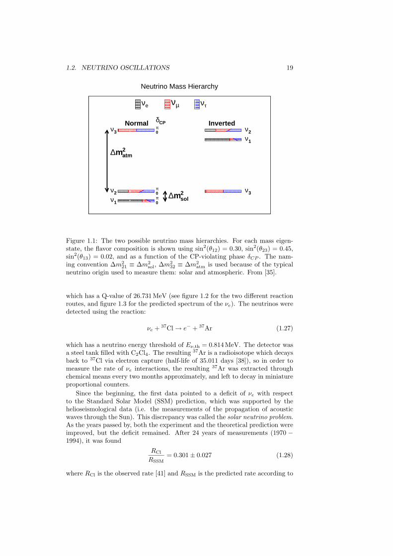
1.2. NEUTRINO OSCILLATIONS 19
eν µν τν
1ν2ν
3ν
1ν2ν
3ν
Normal InvertedCPδπ0
π0π0
atm2m∆
sol2m∆
Neutrino Mass Hierarchy
Figure 1.1: The two possible neutrino mass hierarchies. For each mass eigen-state, the flavor composition is shown using sin2(θ12) = 0.30, sin2(θ23) = 0.45,sin2(θ13) = 0.02, and as a function of the CP-violating phase δCP . The nam-ing convention ∆m2
21 ≡ ∆m2sol, ∆m2
32 ≡ ∆m2atm is used because of the typical
neutrino origin used to measure them: solar and atmospheric. From [35].
which has a Q-value of 26.731 MeV (see figure 1.2 for the two different reactionroutes, and figure 1.3 for the predicted spectrum of the νe). The neutrinos weredetected using the reaction:
νe + 37Cl→ e− + 37Ar (1.27)
which has a neutrino energy threshold of Eν,th = 0.814 MeV. The detector wasa steel tank filled with C2Cl4. The resulting 37Ar is a radioisotope which decaysback to 37Cl via electron capture (half-life of 35.011 days [38]), so in order tomeasure the rate of νe interactions, the resulting 37Ar was extracted throughchemical means every two months approximately, and left to decay in miniatureproportional counters.
Since the beginning, the first data pointed to a deficit of νe with respectto the Standard Solar Model (SSM) prediction, which was supported by thehelioseismological data (i.e. the measurements of the propagation of acousticwaves through the Sun). This discrepancy was called the solar neutrino problem.As the years passed by, both the experiment and the theoretical prediction wereimproved, but the deficit remained. After 24 years of measurements (1970 −1994), it was found
RCl
RSSM= 0.301± 0.027 (1.28)
where RCl is the observed rate [41] and RSSM is the predicted rate according to
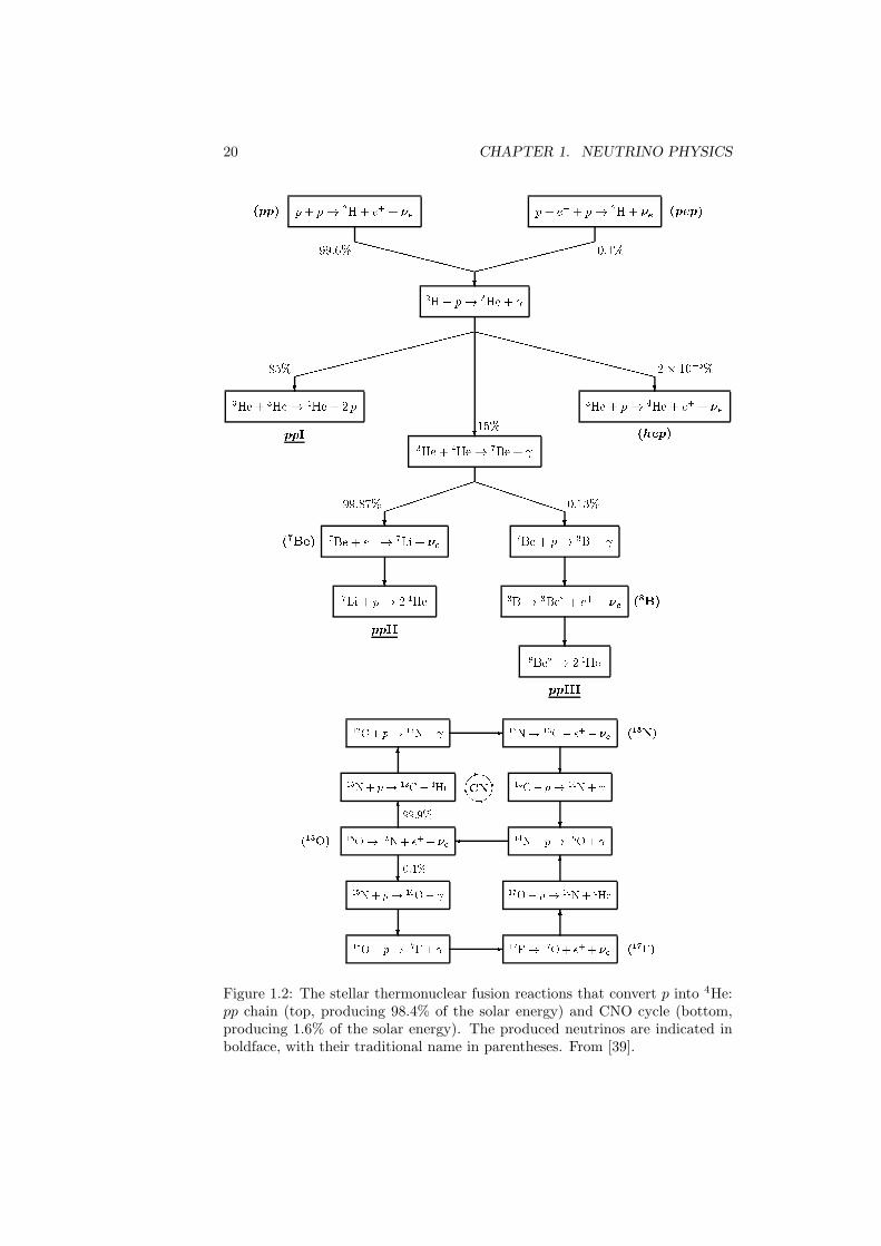
20 CHAPTER 1. NEUTRINO PHYSICS
(pp)
p+ p!
2
H + e
+
+
e
99.6%
X
X
X
X
X
X
X
X
X
X
X
X
(pep)
p+ e
+ p!
2
H +
e
0.4%
?
2
H+ p!
3
He +
85%
?
3
He +
3
He!
4
He + 2 p
ppI
X
X
X
X
X
X
X
X
X
X
X
X
X
X
X
X
XX
2 10
5
%
?
3
He + p!
4
He + e
+
+
e
(hep)
?
15%
3
He +
4
He!
7
Be +
99.87%
?
7
Be + e
!
7
Li +
e
(
7
Be)
?
7
Li + p! 2
4
He
ppII
P
P
P
P
P
P
P
P
P
0.13%
?
7
Be + p!
8
B +
?
8
B!
8
Be
+ e
+
+
e
(
8
B)
?
8
Be
! 2
4
He
ppIII
12
C + p!
13
N+
-
13
N!
13
C + e
+
+
e
(
13
N)
?
13
C + p!
14
N+
?
14
N+ p!
15
O+
15
O!
15
N+ e
+
+
e
(
15
O)
6
15
N + p!
12
C +
4
He
6
CN
-
?
6
?
15
N+ p!
16
O+
?
16
O+ p!
17
F +
-
17
F!
17
O+ e
+
+
e
(
17
F)
6
17
O+ p!
14
N+
4
He
6
99:9%
0:1%
Figure 1.2: The stellar thermonuclear fusion reactions that convert p into 4He:pp chain (top, producing 98.4% of the solar energy) and CNO cycle (bottom,producing 1.6% of the solar energy). The produced neutrinos are indicated inboldface, with their traditional name in parentheses. From [39].
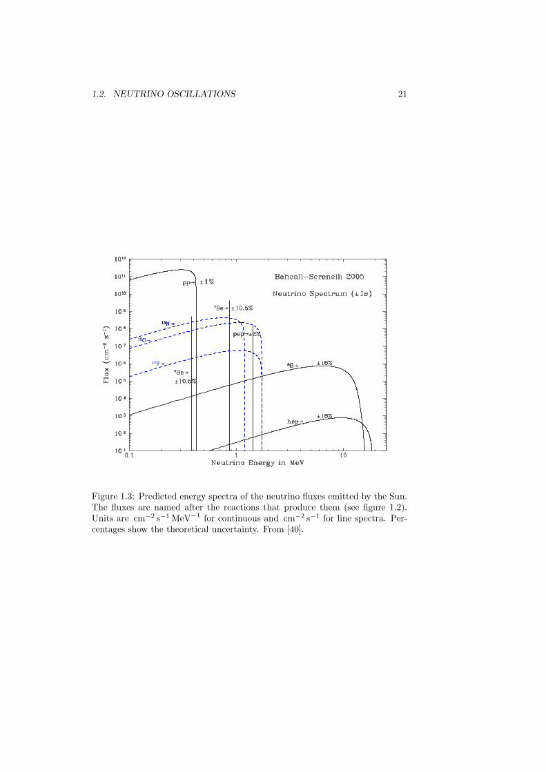
1.2. NEUTRINO OSCILLATIONS 21
Figure 1.3: Predicted energy spectra of the neutrino fluxes emitted by the Sun.The fluxes are named after the reactions that produce them (see figure 1.2).Units are cm−2 s−1 MeV−1 for continuous and cm−2 s−1 for line spectra. Per-centages show the theoretical uncertainty. From [40].
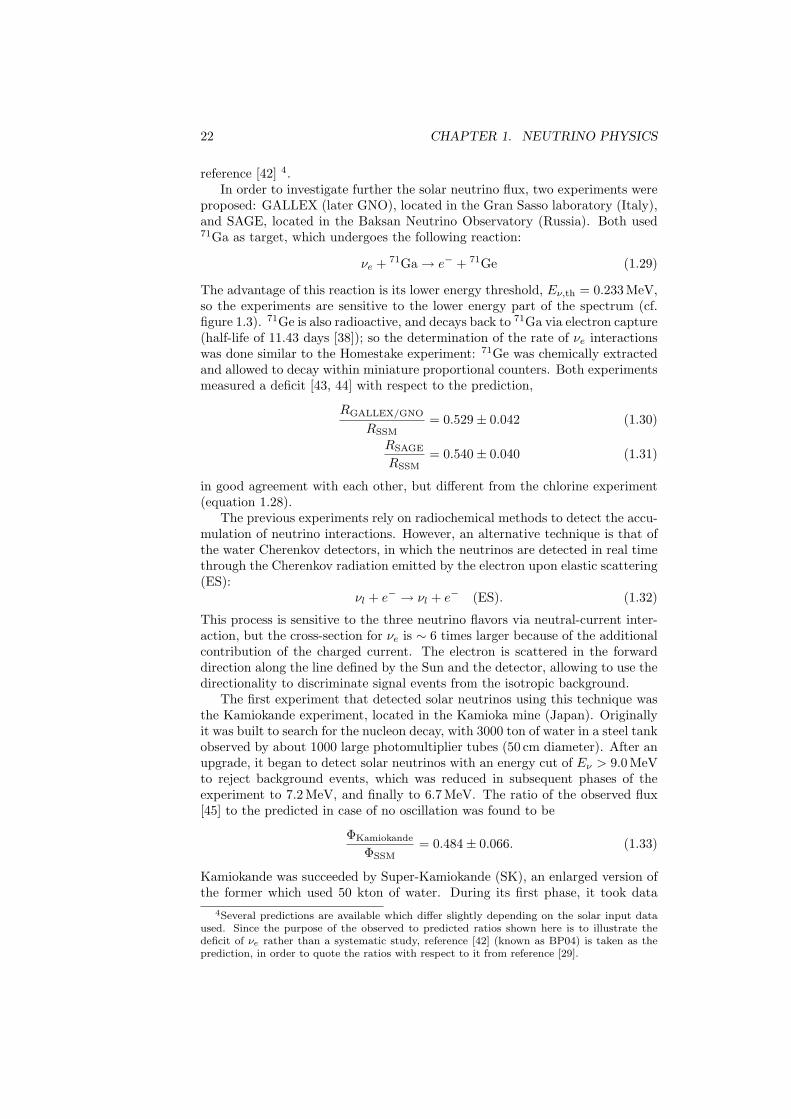
22 CHAPTER 1. NEUTRINO PHYSICS
reference [42] 4.In order to investigate further the solar neutrino flux, two experiments were
proposed: GALLEX (later GNO), located in the Gran Sasso laboratory (Italy),and SAGE, located in the Baksan Neutrino Observatory (Russia). Both used71Ga as target, which undergoes the following reaction:
νe + 71Ga→ e− + 71Ge (1.29)
The advantage of this reaction is its lower energy threshold, Eν,th = 0.233 MeV,so the experiments are sensitive to the lower energy part of the spectrum (cf.figure 1.3). 71Ge is also radioactive, and decays back to 71Ga via electron capture(half-life of 11.43 days [38]); so the determination of the rate of νe interactionswas done similar to the Homestake experiment: 71Ge was chemically extractedand allowed to decay within miniature proportional counters. Both experimentsmeasured a deficit [43, 44] with respect to the prediction,
RGALLEX/GNO
RSSM= 0.529± 0.042 (1.30)
RSAGE
RSSM= 0.540± 0.040 (1.31)
in good agreement with each other, but different from the chlorine experiment(equation 1.28).
The previous experiments rely on radiochemical methods to detect the accu-mulation of neutrino interactions. However, an alternative technique is that ofthe water Cherenkov detectors, in which the neutrinos are detected in real timethrough the Cherenkov radiation emitted by the electron upon elastic scattering(ES):
νl + e− → νl + e− (ES). (1.32)
This process is sensitive to the three neutrino flavors via neutral-current inter-action, but the cross-section for νe is ∼ 6 times larger because of the additionalcontribution of the charged current. The electron is scattered in the forwarddirection along the line defined by the Sun and the detector, allowing to use thedirectionality to discriminate signal events from the isotropic background.
The first experiment that detected solar neutrinos using this technique wasthe Kamiokande experiment, located in the Kamioka mine (Japan). Originallyit was built to search for the nucleon decay, with 3000 ton of water in a steel tankobserved by about 1000 large photomultiplier tubes (50 cm diameter). After anupgrade, it began to detect solar neutrinos with an energy cut of Eν > 9.0 MeVto reject background events, which was reduced in subsequent phases of theexperiment to 7.2 MeV, and finally to 6.7 MeV. The ratio of the observed flux[45] to the predicted in case of no oscillation was found to be
ΦKamiokande
ΦSSM= 0.484± 0.066. (1.33)
Kamiokande was succeeded by Super-Kamiokande (SK), an enlarged version ofthe former which used 50 kton of water. During its first phase, it took data
4Several predictions are available which differ slightly depending on the solar input dataused. Since the purpose of the observed to predicted ratios shown here is to illustrate thedeficit of νe rather than a systematic study, reference [42] (known as BP04) is taken as theprediction, in order to quote the ratios with respect to it from reference [29].
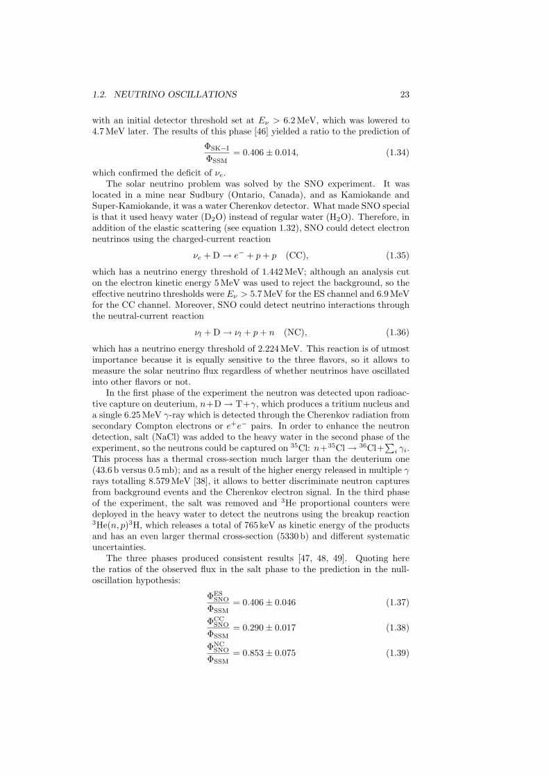
1.2. NEUTRINO OSCILLATIONS 23
with an initial detector threshold set at Eν > 6.2 MeV, which was lowered to4.7 MeV later. The results of this phase [46] yielded a ratio to the prediction of
ΦSK−I
ΦSSM= 0.406± 0.014, (1.34)
which confirmed the deficit of νe.The solar neutrino problem was solved by the SNO experiment. It was
located in a mine near Sudbury (Ontario, Canada), and as Kamiokande andSuper-Kamiokande, it was a water Cherenkov detector. What made SNO specialis that it used heavy water (D2O) instead of regular water (H2O). Therefore, inaddition of the elastic scattering (see equation 1.32), SNO could detect electronneutrinos using the charged-current reaction
νe + D→ e− + p+ p (CC), (1.35)
which has a neutrino energy threshold of 1.442 MeV; although an analysis cuton the electron kinetic energy 5 MeV was used to reject the background, so theeffective neutrino thresholds were Eν > 5.7 MeV for the ES channel and 6.9 MeVfor the CC channel. Moreover, SNO could detect neutrino interactions throughthe neutral-current reaction
νl + D→ νl + p+ n (NC), (1.36)
which has a neutrino energy threshold of 2.224 MeV. This reaction is of utmostimportance because it is equally sensitive to the three flavors, so it allows tomeasure the solar neutrino flux regardless of whether neutrinos have oscillatedinto other flavors or not.
In the first phase of the experiment the neutron was detected upon radioac-tive capture on deuterium, n+D→ T+γ, which produces a tritium nucleus anda single 6.25 MeV γ-ray which is detected through the Cherenkov radiation fromsecondary Compton electrons or e+e− pairs. In order to enhance the neutrondetection, salt (NaCl) was added to the heavy water in the second phase of theexperiment, so the neutrons could be captured on 35Cl: n+35Cl→ 36Cl+
∑i γi.
This process has a thermal cross-section much larger than the deuterium one(43.6 b versus 0.5 mb); and as a result of the higher energy released in multiple γrays totalling 8.579 MeV [38], it allows to better discriminate neutron capturesfrom background events and the Cherenkov electron signal. In the third phaseof the experiment, the salt was removed and 3He proportional counters weredeployed in the heavy water to detect the neutrons using the breakup reaction3He(n, p)3H, which releases a total of 765 keV as kinetic energy of the productsand has an even larger thermal cross-section (5330 b) and different systematicuncertainties.
The three phases produced consistent results [47, 48, 49]. Quoting herethe ratios of the observed flux in the salt phase to the prediction in the null-oscillation hypothesis:
ΦESSNO
ΦSSM= 0.406± 0.046 (1.37)
ΦCCSNO
ΦSSM= 0.290± 0.017 (1.38)
ΦNCSNO
ΦSSM= 0.853± 0.075 (1.39)
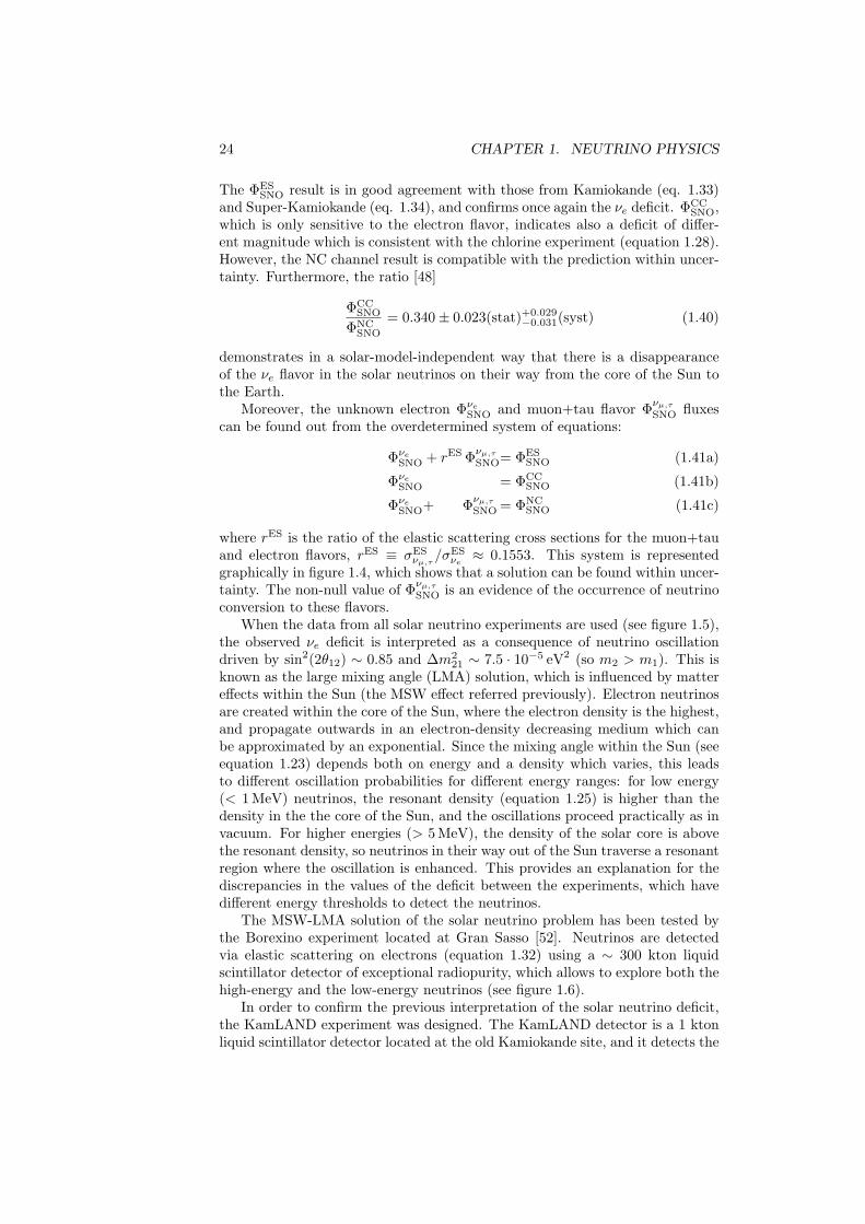
24 CHAPTER 1. NEUTRINO PHYSICS
The ΦESSNO result is in good agreement with those from Kamiokande (eq. 1.33)
and Super-Kamiokande (eq. 1.34), and confirms once again the νe deficit. ΦCCSNO,
which is only sensitive to the electron flavor, indicates also a deficit of differ-ent magnitude which is consistent with the chlorine experiment (equation 1.28).However, the NC channel result is compatible with the prediction within uncer-tainty. Furthermore, the ratio [48]
ΦCCSNO
ΦNCSNO
= 0.340± 0.023(stat)+0.029−0.031(syst) (1.40)
demonstrates in a solar-model-independent way that there is a disappearanceof the νe flavor in the solar neutrinos on their way from the core of the Sun tothe Earth.
Moreover, the unknown electron ΦνeSNO and muon+tau flavor Φνµ,τSNO fluxescan be found out from the overdetermined system of equations:
ΦνeSNO + rES Φνµ,τSNO= ΦESSNO (1.41a)
ΦνeSNO = ΦCCSNO (1.41b)
ΦνeSNO+ Φνµ,τSNO = ΦNCSNO (1.41c)
where rES is the ratio of the elastic scattering cross sections for the muon+tauand electron flavors, rES ≡ σES
νµ,τ /σESνe ≈ 0.1553. This system is represented
graphically in figure 1.4, which shows that a solution can be found within uncer-tainty. The non-null value of Φνµ,τSNO is an evidence of the occurrence of neutrinoconversion to these flavors.
When the data from all solar neutrino experiments are used (see figure 1.5),the observed νe deficit is interpreted as a consequence of neutrino oscillationdriven by sin2(2θ12) ∼ 0.85 and ∆m2
21 ∼ 7.5 · 10−5 eV2 (so m2 > m1). This isknown as the large mixing angle (LMA) solution, which is influenced by mattereffects within the Sun (the MSW effect referred previously). Electron neutrinosare created within the core of the Sun, where the electron density is the highest,and propagate outwards in an electron-density decreasing medium which canbe approximated by an exponential. Since the mixing angle within the Sun (seeequation 1.23) depends both on energy and a density which varies, this leadsto different oscillation probabilities for different energy ranges: for low energy(< 1 MeV) neutrinos, the resonant density (equation 1.25) is higher than thedensity in the the core of the Sun, and the oscillations proceed practically as invacuum. For higher energies (> 5 MeV), the density of the solar core is abovethe resonant density, so neutrinos in their way out of the Sun traverse a resonantregion where the oscillation is enhanced. This provides an explanation for thediscrepancies in the values of the deficit between the experiments, which havedifferent energy thresholds to detect the neutrinos.
The MSW-LMA solution of the solar neutrino problem has been tested bythe Borexino experiment located at Gran Sasso [52]. Neutrinos are detectedvia elastic scattering on electrons (equation 1.32) using a ∼ 300 kton liquidscintillator detector of exceptional radiopurity, which allows to explore both thehigh-energy and the low-energy neutrinos (see figure 1.6).
In order to confirm the previous interpretation of the solar neutrino deficit,the KamLAND experiment was designed. The KamLAND detector is a 1 ktonliquid scintillator detector located at the old Kamiokande site, and it detects the
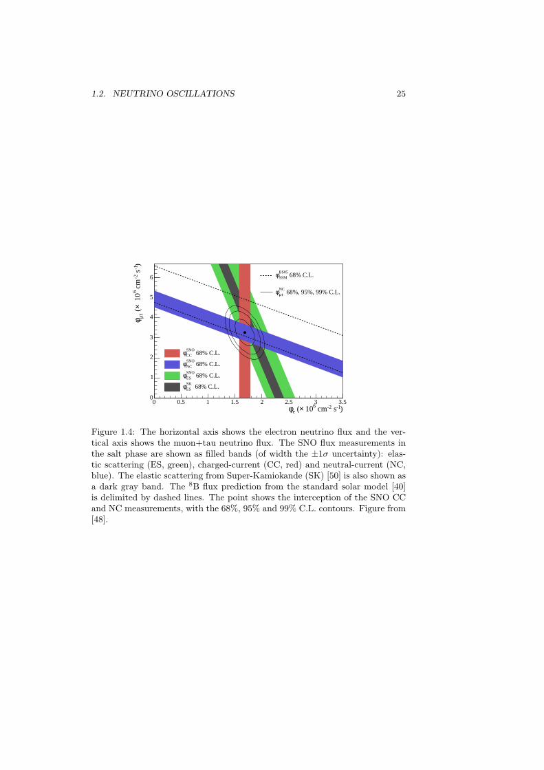
1.2. NEUTRINO OSCILLATIONS 25
)-1 s-2 cm6 10× (eφ0 0.5 1 1.5 2 2.5 3 3.5
)-1
s-2
cm
6 1
0×
( τµφ
0
1
2
3
4
5
6
68% C.L.CCSNOφ
68% C.L.NCSNOφ
68% C.L.ESSNOφ
68% C.L.ESSKφ
68% C.L.SSMBS05φ
68%, 95%, 99% C.L.τµNCφ
Figure 1.4: The horizontal axis shows the electron neutrino flux and the ver-tical axis shows the muon+tau neutrino flux. The SNO flux measurements inthe salt phase are shown as filled bands (of width the ±1σ uncertainty): elas-tic scattering (ES, green), charged-current (CC, red) and neutral-current (NC,blue). The elastic scattering from Super-Kamiokande (SK) [50] is also shown asa dark gray band. The 8B flux prediction from the standard solar model [40]is delimited by dashed lines. The point shows the interception of the SNO CCand NC measurements, with the 68%, 95% and 99% C.L. contours. Figure from[48].
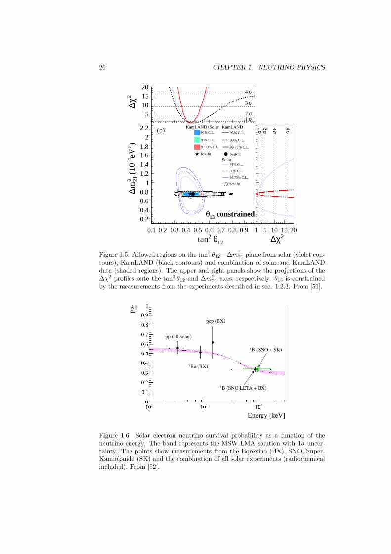
26 CHAPTER 1. NEUTRINO PHYSICS
0.1 0.2 0.3 0.4 0.5 0.6 0.7 0.8 0.9 1
0.20.40.60.8
11.21.41.61.8
22.2 (b)
constrained13θ
12θ 2tan
)2eV
-4 (
10212
m∆KamLAND+Solar KamLAND
Solar
95% C.L.
99% C.L.
99.73% C.L.
best-fit
95% C.L.
99% C.L.
99.73% C.L.
best-fit
95% C.L.
99% C.L.
99.73% C.L.
best-fit
5101520
σ1σ2
σ3
σ4
2 χ∆
5 10 15 20
σ1 σ2 σ3 σ4
2χ∆
Figure 1.5: Allowed regions on the tan2 θ12−∆m221 plane from solar (violet con-
tours), KamLAND (black contours) and combination of solar and KamLANDdata (shaded regions). The upper and right panels show the projections of the∆χ2 profiles onto the tan2 θ12 and ∆m2
21 axes, respectively. θ13 is constrainedby the measurements from the experiments described in sec. 1.2.3. From [51].
pp (all solar) !
7Be (BX)!
pep (BX)!
8B (SNO + SK)!
Energy [keV]!
P ee!
8B (SNO LETA + BX)!
3ν"
Figure 1.6: Solar electron neutrino survival probability as a function of theneutrino energy. The band represents the MSW-LMA solution with 1σ uncer-tainty. The points show measurements from the Borexino (BX), SNO, Super-Kamiokande (SK) and the combination of all solar experiments (radiochemicalincluded). From [52].

1.2. NEUTRINO OSCILLATIONS 27
(km/MeV)eν/E0L
20 30 40 50 60 70 80 90 100
Sur
viva
l Pro
babi
lity
0
0.2
0.4
0.6
0.8
1
eνData - BG - Geo best-fit oscillationν3-
Figure 1.7: Ratio of the observed data in the KamLAND experiment (aftersubtraction of backgrounds and νe produced in the Earth) to the no-oscillationprediction, as a function of L0/E; where L0 = 180 km is the flux-weightedaverage baseline to the reactor cores and E is the νe energy. The blue histogramshows the best fit to a three-flavor survival probability. From [51].
electron antineutrinos emitted from the Japanese nuclear reactors, at an averagedistance of 180 km (with a ∼ 2.5% contribution of Korean reactors and < 1% ofother foreign reactors). The νe are detected using the reaction νe+p→ e+ +n,which is also used by Double Chooz and it is discussed in detail in section 2.2.The survival probability of νe must be equal to that of νe by CPT symmetry,so the solar neutrino deficit can be reproduced using antineutrinos from nuclearreactors. The mean energy of reactor νe is ∼ 4 MeV, which made the experimentsensitive to oscillations driven by ∆m2
21 ∼ O(10−5 eV2), which is the squared-mass difference suggested by the combination of the solar experiments.
For the relevant length traveled by the antineutrinos at KamLAND, theoscillation due to ∆m2
31 is averaged out, and the three-flavor survival probabilitycan be approximated by
Pee(L,E) = cos4(θ13)P 2νee,m(L,E) + sin4(θ13), (1.42)
where P 2νee,m is the two-flavor survival probability in matter and is given by
P 2νee,m(L,E) = 1− sin2(2θ12,m) sin2
(∆m2
21,mL
4E
), (1.43)
where θ12,m and ∆m221,m are the θ12 mixing angle and the ∆m2
21 squared-massdifference in matter, respectively, which can be obtained from equations 1.23and 1.24 and replacing Ne by Ne cos2(2θ13).
KamLAND succeeded in observing an νe deficit. Indeed, it has been able tostudy the νe deficit as a function of the νe energy, demonstrating the oscillatorybehavior which is characteristic of neutrino oscillations, as figure 1.7 shows.
28 CHAPTER 1. NEUTRINO PHYSICS
The combination of the solar experiments, which constrain best θ12, and theKamLAND experiment, which constrains best ∆m2
21, produces the most precisemeasurements of θ12 and ∆m2
21 (see figure 1.5) [51, 10]:
sin2(2θ12) = 0.846± 0.021 (1.44)
∆m221 = (7.53± 0.18) · 10−5 eV2 (1.45)
Leaving θ13 as a free parameter or constraining it by the measurements fromthe experiments introduced in section 1.2.3 does not affect these values.
1.2.2 Measurement of θ23 and |∆m232|
The sequence of experiments that led to the measurement of the θ23 mixingangle and the ∆m2
32 squared-mass difference absolute value (since the sign isstill unknown) was initiated by the atmospheric neutrino anomaly. The atmo-spheric neutrinos are the neutrinos and antineutrinos which are created as aresult of the interaction of primary cosmic rays with atoms in the atmosphere.These energetic collisions generate hadrons, mostly pions (and kaons at higherenergies) which decay dominantly into muons and neutrinos:
π+ → µ+ + νµ, π− → µ− + νµ. (1.46)
The muons themselves decay into electrons (or positrons), producing more neu-trinos:
µ+ → νµ + νe + e+, µ− → νµ + νe + e−. (1.47)
Therefore, at low energies (. 1 GeV) in order to let the muons decay beforereaching the detectors, the expected flavor composition of the atmospheric neu-trino flux is Φ(νµ + νµ) : Φ(νe + νe) ≈ 2 : 1.
An anomalous deficit of the muon-flavor in the atmospheric neutrino flux wasreported by the Kamiokande and IMB experiments [53, 54]. Both experimentswere searching for the nucleon decay with water Cherenkov detectors, and theatmospheric neutrinos represented an undesired background which had to bemodeled. For that reason, efforts were made to produce predictions of the flux.These neutrinos were detected through charged-current interactions with thenuclei in the detector:
νl +N → l− +X, νl +N → l+ +X, (1.48)
in which the lepton is revealed by the Cherenkov radiation emitted. Sincethe detectors were not magnetized, no charge discrimination was possible. Inaddition, tau leptons were very difficult to detect, since they decay almost im-mediately. In order to cancel theoretical and experimental uncertainties, themeasurements can be reported as double ratios between the observed data andthe Monte Carlo prediction, finding for both experiments:
Φ(νµ + νµ)/Φ(νe + νe)∣∣∣DATA
Φ(νµ + νµ)/Φ(νe + νe)∣∣∣MC
≈ 0.6, (1.49)
which shows a clear discrepancy with respect to the prediction.
1.2. NEUTRINO OSCILLATIONS 29
The atmospheric neutrino flux was precisely measured by the Super-Kamio-kande experiment (already introduced in the context of solar neutrinos) as afunction of the distance L traveled (inferred from the zenith angle Θ) and theneutrino energy (see figure 1.8). The Cherenkov detection technique providesdirectional information which allows to distinguish if the neutrinos come directlyfrom above (downward charged leptons), cos Θ ≈ 1 and L ∼ 20 km, or havecrossed the Earth on their way to the detector (upward charged leptons), cos Θ ≈−1 and L ∼ 13000 km. Super-Kamiokande found a deficit in the muon neutrinoswith respect to the no-oscillation prediction which increased with the distancetraveled by the neutrino, while the electron neutrinos agreed with the prediction.Therefore, the result was interpreted as νµ → ντ oscillation. Since νµ and ντinteract equally with the Earth, no matter effects apply. Neglecting the small∆m2
21, the νµ survival probability can be approximated by:
Pµµ(L,E) ≈ 1−4 cos2(θ13) sin2(θ23)[1− cos2(θ13) sin2(θ23)
]×
× sin2
(1.27
∆m2atm[ eV2]L[ km]E[ GeV]
),
(1.50)
where ∆m2atm = ∆m2
32 for normal mass hierarchy or ∆m2atm = ∆m2
13 for in-verted mass hierarchy, and the oscillatory phase is written in the usual units usedby these experiments. The analysis of the Super-Kamiokande data [55] foundthe best fit at sin2(θ23) = 0.5, ∆m2
atm = 2.1 · 10−3 eV2 and sin2(θ13) = 0.0.Similar results were found by the Soudan 2 experiment [56], a 960 ton irontracking calorimeter placed at the Soudan mine (Minnesota, USA); and by theMACRO experiment [57], using scintillator counters and streamer tubes, whichwas located at the Gran Sasso laboratory.
As in the case of the solar neutrinos, in order to reproduce the muon-flavordeficit observed in the atmospheric neutrinos, human-made neutrinos were used.Muon neutrino beams can be produced colliding protons with an energy of sev-eral GeV against a fixed target, creating secondary hadron showers. A magneticdevice called horn focuses the resulting pions and kaons, which are allowed todecay in flight for ∼ 100 m until they are stopped by an absorber material. Theresulting beam is composed mostly of muon neutrinos with a small componentof electron neutrinos. The beam energy is typically of a few GeV, so in order toexplore squared-mass differences such as the atmospheric one of O(10−3 eV2),baselines of several hundreds of kilometers are required.
The K2K experiment was the first long-baseline experiment which used thiskind of beam. A 〈Eν〉 ∼ 1.3 GeV beam was produced at the KEK proton syn-chrotron and sent towards the Super-Kamiokande detector. The neutrino flux,energy spectrum and profile of the beam were measured by a near multi-detectorsystem at ∼ 300 m from the production target. Even though the baseline wasnot optimal, L = 250 km, determined by the pre-existing locations of KEK andSuper-Kamiokande, the K2K experiment confirmed the oscillation parametersobtained from the atmospheric neutrinos [58].
The second long-baseline experiment built is the MINOS experiment. Theneutrino beam, peaked at ∼ 3 GeV, is produced using the protons extractedfrom the Main Injector at the Fermi National Accelerator Laboratory and senttowards a far detector located 735 km away from the target, in the Soudan mine.A near detector 1 km downstream the target characterizes the neutrino beambefore the oscillation is developed, in order to predict the unoscillated flux and
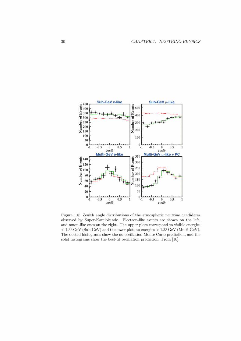
30 CHAPTER 1. NEUTRINO PHYSICS
0
50
100
150
200
250
300
350
400
450
-1 -0.5 0 0.5 1
cosΘ
Nu
mb
er o
f E
ven
ts
Sub-GeV e-like
0
100
200
300
400
500
-1 -0.5 0 0.5 1
cosΘ
Nu
mb
er o
f E
ven
ts
Sub-GeV μ-like
0
20
40
60
80
100
120
140
-1 -0.5 0 0.5 1
cosΘ
Nu
mb
er o
f E
ven
ts
Multi-GeV e-like
0
50
100
150
200
250
300
350
-1 -0.5 0 0.5 1
cosΘ
Nu
mb
er o
f E
ven
ts
Multi-GeV μ-like + PC
Figure 1.8: Zenith angle distributions of the atmospheric neutrino candidatesobserved by Super-Kamiokande. Electron-like events are shown on the left,and muon-like ones on the right. The upper plots correspond to visible energies< 1.33 GeV (Sub-GeV) and the lower plots to energies > 1.33 GeV (Multi-GeV).The dotted histograms show the no-oscillation Monte Carlo prediction, and thesolid histograms show the best-fit oscillation prediction. From [10].
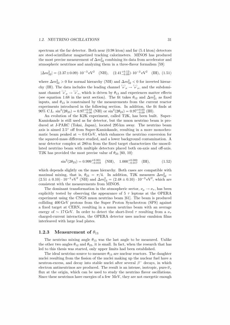
1.2. NEUTRINO OSCILLATIONS 31
spectrum at the far detector. Both near (0.98 kton) and far (5.4 kton) detectorsare steel-scintillator magnetized tracking calorimeters. MINOS has producedthe most precise measurement of ∆m2
32 combining its data from accelerator andatmospheric neutrinos and analyzing them in a three-flavor formalism [59]:
|∆m232| = (2.37±0.09) ·10−3 eV2 (NH), (2.41+0.12
−0.09) ·10−3 eV2 (IH), (1.51)
where ∆m232 > 0 for normal hierarchy (NH) and ∆m2
32 < 0 for inverted hierar-chy (IH). The data includes the leading channel
(−)ν µ →
(−)ν µ, and the subdomi-
nant channel(−)ν µ →
(−)ν e, which is driven by θ13 and experiences matter effects
(see equation 1.68 in the next section). The fit takes θ12 and ∆m221 as fixed
inputs, and θ13 is constrained by the measurements from the current reactorexperiments introduced in the following section. In addition, the fit finds at90% C.L. sin2(2θ23) = 0.97+0.03
−0.06 (NH) or sin2(2θ23) = 0.97+0.03−0.09 (IH).
An evolution of the K2K experiment, called T2K, has been built. Super-Kamiokande is still used as far detector, but the muon neutrino beam is pro-duced at J-PARC (Tokai, Japan), located 295 km away. The neutrino beamaxis is aimed 2.5 off from Super-Kamiokande, resulting in a more monochro-matic beam peaked at ∼ 0.6 GeV, which enhances the neutrino conversion forthe squared-mass difference studied, and a lower background contamination. Anear detector complex at 280 m from the fixed target characterizes the unoscil-lated neutrino beam with multiple detectors placed both on-axis and off-axis.T2K has provided the most precise value of θ23 [60, 10]:
sin2(2θ23) = 0.999+0.001−0.018 (NH), 1.000+0.000
−0.017 (IH), (1.52)
which depends slightly on the mass hierarchy. Both cases are compatible withmaximal mixing, that is, θ23 = π/4. In addition, T2K measures ∆m2
32 =(2.51 ± 0.10) · 10−3 eV2 (NH) and ∆m2
13 = (2.48 ± 0.10) · 10−3 eV2, which areconsistent with the measurements from MINOS.
The dominant transformation in the atmospheric sector, νµ → ντ , has beenexplicitly tested by observing the appearance of 5 τ leptons at the OPERAexperiment using the CNGS muon neutrino beam [61]. The beam is producedcolliding 400 GeV protons from the Super Proton Synchrotron (SPS) againsta fixed target at CERN, resulting in a muon neutrino beam with an averageenergy of ∼ 17 GeV. In order to detect the short-lived τ resulting from a ντcharged-current interaction, the OPERA detector uses nuclear emulsion filmsinterleaved with large lead plates.
1.2.3 Measurement of θ13
The neutrino mixing angle θ13 was the last angle to be measured. Unlikethe other two angles θ12 and θ23, it is small. In fact, when the research that hasled to this thesis was started, only upper limits had been established.
The ideal neutrino source to measure θ13 are nuclear reactors. The daughternuclei resulting from the fission of the nuclei making up the nuclear fuel have aneutron-excess, and decay into stable nuclei after several β− decays, in whichelectron antineutrinos are produced. The result is an intense, isotropic, pure-νeflux at the origin, which can be used to study the neutrino flavor oscillations.Since these neutrinos have energies of a few MeV, they are not energetic enough
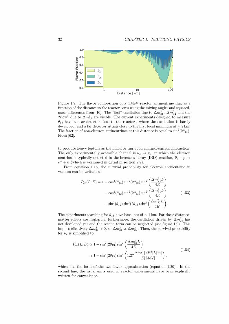
32 CHAPTER 1. NEUTRINO PHYSICS
1 10 100Distance [km]
0.0
0.2
0.4
0.6
0.8
1.0
Flavor
Fract
ion
νe
νµ
ντ
Figure 1.9: The flavor composition of a 4 MeV reactor antineutrino flux as afunction of the distance to the reactor cores using the mixing angles and squared-mass differences from [10]. The “fast” oscillation due to ∆m2
31, ∆m232 and the
“slow” due to ∆m221 are visible. The current experiments designed to measure
θ13 have a near detector close to the reactors, where the oscillation is barelydeveloped, and a far detector sitting close to the first local minimum at ∼ 2 km.The fraction of non-electron antineutrinos at this distance is equal to sin2(2θ13).From [62].
to produce heavy leptons as the muon or tau upon charged-current interaction.The only experimentally accessible channel is νe → νe, in which the electronneutrino is typically detected in the inverse β-decay (IBD) reaction, νe + p →e+ + n (which is examined in detail in section 2.2).
From equation 1.16, the survival probability for electron antineutrino invacuum can be written as
Pee(L,E) = 1− cos4(θ13) sin2(2θ12) sin2
(∆m2
21L
4E
)− cos2(θ12) sin2(2θ13) sin2
(∆m2
31L
4E
)− sin2(θ12) sin2(2θ13) sin2
(∆m2
32L
4E
).
(1.53)
The experiments searching for θ13 have baselines of ∼ 1 km. For these distancesmatter effects are negligible; furthermore, the oscillation driven by ∆m2
21 hasnot developed yet and the second term can be neglected (see figure 1.9). Thisimplies effectively ∆m2
21 ≈ 0, so ∆m231 ' ∆m2
32. Then, the survival probabilityfor νe is simplified to
Pee(L,E) ' 1− sin2(2θ13) sin2
(∆m2
31L
4E
)≈ 1− sin2(2θ13) sin2
(1.27
∆m231[ eV2]L[ m]E[ MeV]
),
(1.54)
which has the form of the two-flavor approximation (equation 1.20). In thesecond line, the usual units used in reactor experiments have been explicitlywritten for convenience.
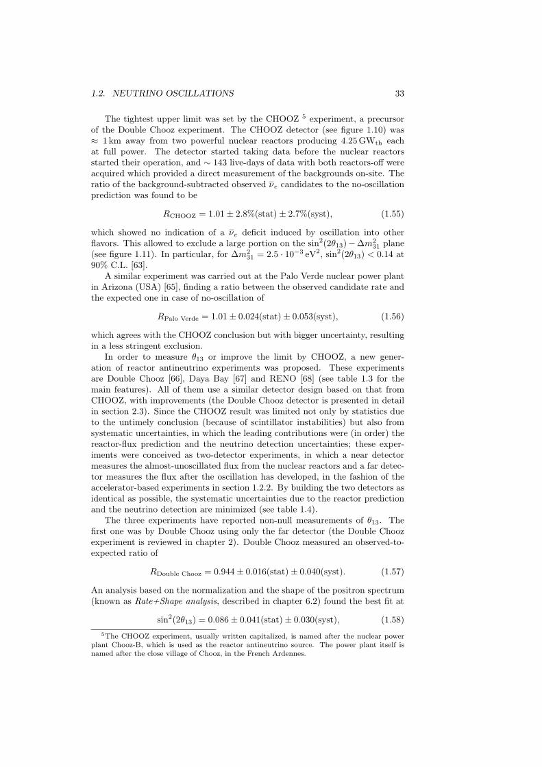
1.2. NEUTRINO OSCILLATIONS 33
The tightest upper limit was set by the CHOOZ 5 experiment, a precursorof the Double Chooz experiment. The CHOOZ detector (see figure 1.10) was≈ 1 km away from two powerful nuclear reactors producing 4.25 GWth eachat full power. The detector started taking data before the nuclear reactorsstarted their operation, and ∼ 143 live-days of data with both reactors-off wereacquired which provided a direct measurement of the backgrounds on-site. Theratio of the background-subtracted observed νe candidates to the no-oscillationprediction was found to be
RCHOOZ = 1.01± 2.8%(stat)± 2.7%(syst), (1.55)
which showed no indication of a νe deficit induced by oscillation into otherflavors. This allowed to exclude a large portion on the sin2(2θ13)−∆m2
31 plane(see figure 1.11). In particular, for ∆m2
31 = 2.5 · 10−3 eV2, sin2(2θ13) < 0.14 at90% C.L. [63].
A similar experiment was carried out at the Palo Verde nuclear power plantin Arizona (USA) [65], finding a ratio between the observed candidate rate andthe expected one in case of no-oscillation of
RPalo Verde = 1.01± 0.024(stat)± 0.053(syst), (1.56)
which agrees with the CHOOZ conclusion but with bigger uncertainty, resultingin a less stringent exclusion.
In order to measure θ13 or improve the limit by CHOOZ, a new gener-ation of reactor antineutrino experiments was proposed. These experimentsare Double Chooz [66], Daya Bay [67] and RENO [68] (see table 1.3 for themain features). All of them use a similar detector design based on that fromCHOOZ, with improvements (the Double Chooz detector is presented in detailin section 2.3). Since the CHOOZ result was limited not only by statistics dueto the untimely conclusion (because of scintillator instabilities) but also fromsystematic uncertainties, in which the leading contributions were (in order) thereactor-flux prediction and the neutrino detection uncertainties; these exper-iments were conceived as two-detector experiments, in which a near detectormeasures the almost-unoscillated flux from the nuclear reactors and a far detec-tor measures the flux after the oscillation has developed, in the fashion of theaccelerator-based experiments in section 1.2.2. By building the two detectors asidentical as possible, the systematic uncertainties due to the reactor predictionand the neutrino detection are minimized (see table 1.4).
The three experiments have reported non-null measurements of θ13. Thefirst one was by Double Chooz using only the far detector (the Double Choozexperiment is reviewed in chapter 2). Double Chooz measured an observed-to-expected ratio of
RDouble Chooz = 0.944± 0.016(stat)± 0.040(syst). (1.57)
An analysis based on the normalization and the shape of the positron spectrum(known as Rate+Shape analysis, described in chapter 6.2) found the best fit at
sin2(2θ13) = 0.086± 0.041(stat)± 0.030(syst), (1.58)5The CHOOZ experiment, usually written capitalized, is named after the nuclear power
plant Chooz-B, which is used as the reactor antineutrino source. The power plant itself isnamed after the close village of Chooz, in the French Ardennes.
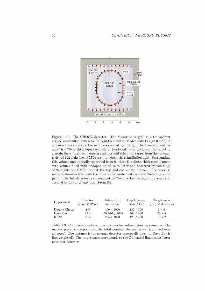
34 CHAPTER 1. NEUTRINO PHYSICS
veto
acrylicvessel
neutrinotarget
opticalbarrier
low activity gravel shielding
containmentregion
steeltank
Figure 1.10: The CHOOZ detector. The “neutrino target” is a transparentacrylic vessel filled with 5 ton of liquid scintillator loaded with Gd (at 0.09%) toenhance the capture of the neutrons created by the νe. The “containment re-gion” is a 70 cm thick liquid scintillator (undoped) layer enclosing the target tocontain the γ-rays from neutron captures and shield the target from the radioac-tivity of 192 eight-inch PMTs used to detect the scintillation light. Surroundingthis volume and optically separated from it, there is a 80 cm thick cosmic muonveto volume filled with undoped liquid scintillator and observed by two ringsof 24 eight-inch PMTs, one at the top and one at the bottom. The vessel ismade of stainless steel with the inner walls painted with a high-reflectivity whitepaint. The full detector is surrounded by 75 cm of low radioactivity sand andcovered by 14 cm of cast iron. From [64].
ExperimentReactor Distance (m) Depth (mwe) Target mass
power (GWth) Near / Far Near / Far (ton) × detectors
Double Chooz 8.5 400 / 1050 120 / 300 8× 2Daya Bay 17.4 470, 576 / 1648 260 / 860 20× 8RENO 16.5 294 / 1383 120 / 450 16× 2
Table 1.3: Comparison between current reactor antineutrino experiments. Thereactor power corresponds to the total nominal thermal power (summed overall cores). The distance is the average detector-reactor distance (in Daya Bay isflux-weighted). The target mass corresponds to the Gd-loaded liquid scintillatormass per detector.
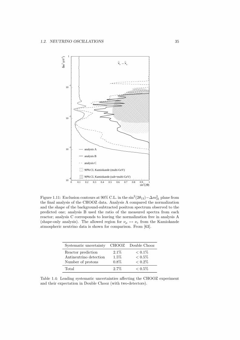
1.2. NEUTRINO OSCILLATIONS 35
10-4
10-3
10-2
10-1
1
0 0.1 0.2 0.3 0.4 0.5 0.6 0.7 0.8 0.9 1sin2(2θ)
δm2 (
eV2 )
analysis A
90% CL Kamiokande (multi-GeV)
90% CL Kamiokande (sub+multi-GeV)
νe → νx
_ _
analysis B
analysis C
Figure 1.11: Exclusion contours at 90% C.L. in the sin2(2θ13)−∆m231 plane from
the final analysis of the CHOOZ data. Analysis A compared the normalizationand the shape of the background-subtracted positron spectrum observed to thepredicted one; analysis B used the ratio of the measured spectra from eachreactor; analysis C corresponds to leaving the normalization free in analysis A(shape-only analysis). The allowed region for νµ ↔ νe from the Kamiokandeatmospheric neutrino data is shown for comparison. From [63].
Systematic uncertainty CHOOZ Double Chooz
Reactor prediction 2.1% < 0.1%Antineutrino detection 1.5% < 0.5%Number of protons 0.8% < 0.2%
Total 2.7% < 0.5%
Table 1.4: Leading systematic uncertainties affecting the CHOOZ experimentand their expectation in Double Chooz (with two-detectors).
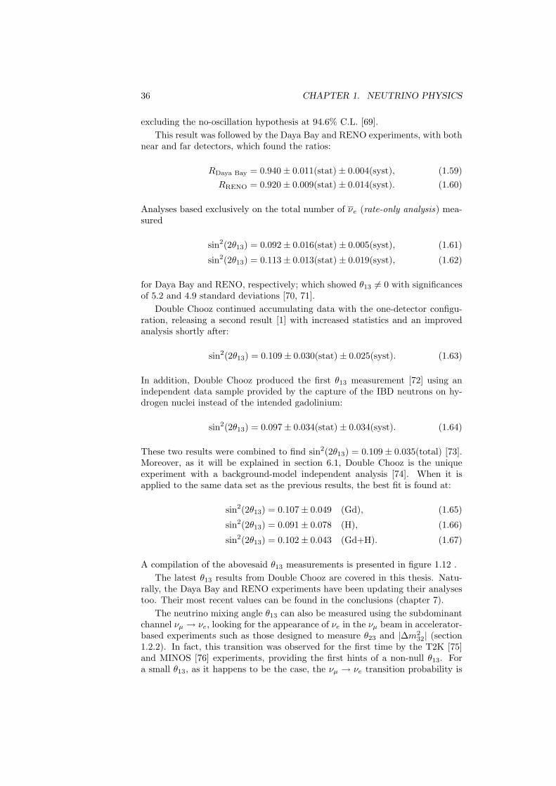
36 CHAPTER 1. NEUTRINO PHYSICS
excluding the no-oscillation hypothesis at 94.6% C.L. [69].This result was followed by the Daya Bay and RENO experiments, with both
near and far detectors, which found the ratios:
RDaya Bay = 0.940± 0.011(stat)± 0.004(syst), (1.59)RRENO = 0.920± 0.009(stat)± 0.014(syst). (1.60)
Analyses based exclusively on the total number of νe (rate-only analysis) mea-sured
sin2(2θ13) = 0.092± 0.016(stat)± 0.005(syst), (1.61)
sin2(2θ13) = 0.113± 0.013(stat)± 0.019(syst), (1.62)
for Daya Bay and RENO, respectively; which showed θ13 6= 0 with significancesof 5.2 and 4.9 standard deviations [70, 71].
Double Chooz continued accumulating data with the one-detector configu-ration, releasing a second result [1] with increased statistics and an improvedanalysis shortly after:
sin2(2θ13) = 0.109± 0.030(stat)± 0.025(syst). (1.63)
In addition, Double Chooz produced the first θ13 measurement [72] using anindependent data sample provided by the capture of the IBD neutrons on hy-drogen nuclei instead of the intended gadolinium:
sin2(2θ13) = 0.097± 0.034(stat)± 0.034(syst). (1.64)
These two results were combined to find sin2(2θ13) = 0.109± 0.035(total) [73].Moreover, as it will be explained in section 6.1, Double Chooz is the uniqueexperiment with a background-model independent analysis [74]. When it isapplied to the same data set as the previous results, the best fit is found at:
sin2(2θ13) = 0.107± 0.049 (Gd), (1.65)
sin2(2θ13) = 0.091± 0.078 (H), (1.66)
sin2(2θ13) = 0.102± 0.043 (Gd+H). (1.67)
A compilation of the abovesaid θ13 measurements is presented in figure 1.12 .The latest θ13 results from Double Chooz are covered in this thesis. Natu-
rally, the Daya Bay and RENO experiments have been updating their analysestoo. Their most recent values can be found in the conclusions (chapter 7).
The neutrino mixing angle θ13 can also be measured using the subdominantchannel νµ → νe, looking for the appearance of νe in the νµ beam in accelerator-based experiments such as those designed to measure θ23 and |∆m2
32| (section1.2.2). In fact, this transition was observed for the first time by the T2K [75]and MINOS [76] experiments, providing the first hints of a non-null θ13. Fora small θ13, as it happens to be the case, the νµ → νe transition probability is
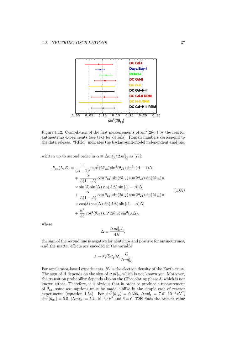
1.2. NEUTRINO OSCILLATIONS 37
)13θ(22sin0.00 0.05 0.10 0.15 0.20 0.25 0.30
DC Gd-I
Daya Bay-I
RENO-I
DC Gd-II
DC H-II
DC Gd+H-II
DC Gd-II RRM
DC H-II RRM
DC Gd+H-II RRM
DC Gd-I
Daya Bay-I
RENO-I
DC Gd-II
DC H-II
DC Gd+H-II
DC Gd-II RRM
DC H-II RRM
DC Gd+H-II RRM
Figure 1.12: Compilation of the first measurements of sin2(2θ13) by the reactorantineutrino experiments (see text for details). Roman numbers correspond tothe data release. “RRM” indicates the background-model independent analysis.
written up to second order in α ≡ ∆m221/∆m
232 as [77]:
Pµe(L,E) =1
(A− 1)2sin2(2θ13) sin2(θ23) sin2 [(A− 1)∆]
∓ α
A(1−A)cos(θ13) sin(2θ12) sin(2θ23) sin(2θ13)×
× sin(δ) sin(∆) sin(A∆) sin [(1−A)∆]
+α
A(1−A)cos(θ13) sin(2θ12) sin(2θ23) sin(2θ13)×
× cos(δ) cos(∆) sin(A∆) sin [(1−A)∆]
+α2
A2cos2(θ23) sin2(2θ12) sin2(A∆),
(1.68)
where
∆ ≡ ∆m232L
4E,
the sign of the second line is negative for neutrinos and positive for antineutrinos,and the matter effects are encoded in the variable
A ≡ 2√
2GFNeE
∆m232
.
For accelerator-based experiments, Ne is the electron density of the Earth crust.The sign of A depends on the sign of ∆m2
32, which is not known yet. Moreover,the transition probability depends also on the CP-violating phase δ, which is notknown either. Therefore, it is obvious that in order to produce a measurementof θ13, some assumptions must be made, unlike in the simple case of reactorexperiments (equation 1.54). For sin2(θ12) = 0.306, ∆m2
21 = 7.6 · 10−5 eV2,sin2(θ23) = 0.5, |∆m2
32| = 2.4 · 10−3 eV2 and δ = 0, T2K finds the best-fit value
38 CHAPTER 1. NEUTRINO PHYSICS
)π (
CP
δ68% CL90% CLBest fit
rangeσPDG2012 1
>0322m∆
-1
-0.5
0
0.5
1
13θ22sin0 0.05 0.1 0.15 0.2 0.25 0.3 0.35 0.4
)π (
CP
δ
<0322m∆
-1
-0.5
0
0.5
1
Figure 1.13: 68% and 90% allowed regions on the sin2(2θ13)−δ plane for normalhierarchy (top) and inverted hierarchy (bottom). The best fit for sin2(2θ13) forthe given value of δ is shown as a solid line. θ23 and |∆m2
32| are varied in the fitconstrained by the T2K own measurements. The vertical shaded region showsthe average sin2(2θ13) from the PDG2012 sin2(2θ13) = 0.098± 0.013. From [78]and references therein.
at [78]
sin2(2θ13) = 0.140+0.038−0.032 (NH), (1.69)
sin2(2θ13) = 0.170+0.045−0.037 (IH), (1.70)
where, as usual, NH stands for normal mass hierarchy (∆m232 > 0) and IH for
inverted mass hierarchy (∆m232 < 0).
Nevertheless, although the dependence on the CP-violating phase δ is coun-terproductive for a clean measurement of θ13 by accelerator-based experiments,it has provided the first glimpse of the value of δ when the input from thereactors experiment on θ13 is used, as figure 1.13 shows. The preferred valueis δ = π/2, i.e. maximal CP violation, but the uncertainties are still large.However, δ values in the interval (0.19π, 0.80π) in the normal hierarchy, andin (π, 0.97π) and (−0.04π, π) in the inverted hierarchy, are already excluded at90% C.L.
1.3. SEARCH FOR NEUTRINO MASS 39
1.3 Search for neutrino mass
Neutrino oscillation experiments tell us about the differences between thesquared masses of the neutrino mass eigenstates, but only set a lower limit onthe absolute mass scale: if the lightest neutrino mass is taken to be zero andusing the squared-mass differences from [10], then for normal hierarchy:
m2 ≥√
∆m221 = 0.0087± 0.0001 eV (1.71)
and
m3 ≥√
∆m232 + ∆m2
21 = 0.0502± 0.0006 eV; (1.72)
and for inverted hierarchy:
m1 ≥√|∆m2
32| −∆m221 = 0.0494± 0.0007 eV (1.73)
and
m2 ≥√|∆m2
32| = 0.0502± 0.0007 eV; (1.74)
In order to try to measure the absolute neutrino masses, other kinds of experi-ments must be carried out.
1.3.1 Kinematic limits
The mass of the neutrinos can be deduced from the conservation of energyand momentum in weak interactions involving neutrinos, providing a directmeasurement.
In the β− decay, the endpoint of the electron spectrum, which correspondsto the maximum kinetic energy carried away by the electron, Tmax, is sensitiveto the electron antineutrino mass, mνe :
Tmax = Qβ −mνe , (1.75)
where Qβ = Mi −Mf − me is the Q-value of the reaction, with Mi and Mf
the masses of the initial and final nuclei, and me the mass of the electron. Inorder to study this effect, nuclei with low Q-values are preferable to maximizethe number of events at the endpoint. A good candidate is tritium, with aQ-value of 18.6 keV and a half-life of 12.3 years. Nevertheless, as a result of theneutrino mixing, νe has not a definite mass. Then, the β− decay of tritium isan incoherent (because of the different final states) sum of decay modes:
3H→ 3He + e− + νj , (1.76)
where νj are the antineutrino mass eigenstates. Therefore, the endpoint of theelectron spectrum will exhibit a shift from the massless neutrinos case Tmax =Qβ to Tmax = Qβ−min(mj), where min(mj) is the lightest mass, with additionalkinks at T = Qβ −mk, with mk 6= min(mj).
40 CHAPTER 1. NEUTRINO PHYSICS
However, measuring the shift and the kinks is very difficult since the rate ofevents close to the endpoint energy tends to zero. Instead, it is more practicalto measure deviations in the Kurie function defined as
K(T ) ≡
(Qβ − T )3∑j=1
|Uej |2√
(Qβ − T )2 −m2j
12
, (1.77)
where T is the kinetic energy of the emitted electron and Uej is the j-th matrixelement from the electron-neutrino row of the PMNS matrix (equation 1.5). Ifthe resolution of the experimental apparatus is such that it cannot resolve theindividual masses, the Kurie plot can be approximated considering Qβ − T >>mj to
K(T ) '[(Qβ − T )
√(Qβ − T )2 −m2
β
] 12, (1.78)
where mβ
mβ =
3∑j=1
|Uej |2m2j
12
=[c212c
213m
21 + s2
12c213m
22 + s2
13m23
] 12
(1.79)
is the effective electron antineutrino mass in β− decay (which is equal to theelectron neutrino mass if CPT symmetry holds).
No β− decay experiment has measured a neutrino mass different from zeroyet. The best upper limits come from the Troitsk [79] and Mainz [80] β−
spectrometers:
mβ < 2.05 eV (Troitsk) (1.80)mβ < 2.3 eV (Mainz) (1.81)
at 95% C.L. Both collaborations have merged to perform an improved experi-ment in the near future, KATRIN, which will reach a sensitivity of 0.2 eV (90%C.L.) [81].
Less stringent limits have been set to the effective muon and tau neutrinomasses, (meff
νµ)2 =∑3j=1 |Uµj |2m2
j and (meffντ )2 =
∑3j=1 |Uτj |2m2
j . In the case ofthe muon neutrino, the analysis of the decay π+ → µ+ + νµ [82] results in
meffνµ < 0.17 MeV (90% C.L.). (1.82)
For the tau neutrino, the analysis of the channels τ− → 2π−π+ντ and τ− →3π−2π+(π0)ντ [83] gives
meffντ < 18.2 MeV (95% C.L.). (1.83)
1.3.2 Neutrinoless double beta decay
In section 1.1, the mechanism of Higgs-induced neutrino masses was putforward. However, this is not the only possibility. If right-handed neutrinosexist, since they are not charged under any of the Standard Model interactions,
1.3. SEARCH FOR NEUTRINO MASS 41
another possibility to generate neutrino masses is given by (considering only oneneutrino for simplicity, again):
LMajoranamass = −1
2νRM
νMν
CR + H.c., (1.84)
where the charge-conjugated field νCR = CνRT , with C the charge conjugation
operator, is left-handed (i.e. the right-handed projector PR gives PRνCR = 0);
and MνM is its Majorana mass 6.
This second mechanism of mass generation is attractive because it offers aplausible explanation to the smallness of the neutrino mass. If both Dirac andMajorana terms are present, the most general neutrino mass term is written
LDirac+Majoranamass = −νRM
νDνL −
12νRM
νMν
CR + H.c.
= −12NT
L C†MNL,
(1.85)
where
NL =(νL
νCR
), (1.86)
and the mass matrix
M =(
0 MνD
MνD Mν
M
). (1.87)
When the mass matrix is diagonalized, the two eigenvalues result:
mlight '(Mν
D)2
MνM
(1.88)
mheavy 'MνM (1.89)
Since the right-handed neutrino fields are singlets under the Standard Modelgauge symmetries, their Majorana mass is not linked to the electroweak sym-metry breaking scale and can take any value, in particular Mν
M >> MνD. Hence,
even if the left-handed neutrinos fields have a Yukawa coupling which is similarto that of the charged fermions; two very different neutrinos would arise: a lightone (mostly left-handed, the one we are familiar with) with mass mlight << Mf
D,and a heavy one (mostly right-handed, and thereby sterile) with mass mheavy.These neutrinos are Majorana fermions, that is, they are their own antiparticle.This mechanism is known as the seesaw mechanism [84, 85, 86, 87, 88]: theheavier the heavy neutrinos, the lighter the light ones.
A Majorana mass term violates the total lepton number symmetry of theStandard Model by two units. This allows to test experimentally the Majorananeutrino hypothesis, since if such term is present, neutrinoless double β decay(ββ0ν) should occur:
AZ X→ A
Z±2Y + 2e∓. (1.90)
6No renormalizable Majorana term can be built with νL in the Standard Model becauseit would require a weak isospin Higgs triplet with Y = 2 which is absent. However, if theStandard Model is regarded as a low-energy effective theory and renormalizability is given up,a Majorana mass term using the Standard Model Higgs doublet would be possible, resultingin a mass Mν
M = κv2/Λ, where κ is a dimensionless coupling constant and Λ is a heavy masscharacteristic of the symmetry-breaking scale of the new physics.
42 CHAPTER 1. NEUTRINO PHYSICS
The simplest realization of this process consists in the exchange of a virtual lightMajorana neutrino between the two virtual W∓ bosons emitted by the decayingnucleons 7. In this case, the half-life of the process for the nucleus X is written:
T 0ν1/2(X) =
[G0νX
∣∣M0νX
∣∣2(mββ
me
)2]−1
, (1.91)
where G0νX and M0ν
X are a phase space factor and a nuclear matrix elementwhich depend on the nucleus, respectively. While G0ν
X can be calculated pre-cisely, the calculation of M0ν
X requires to rely on a nuclear model, introducingconsiderable theoretical uncertainty. mββ is the effective Majorana mass, whichis the coherent sum of the masses of the neutrino mass eigenstates, mj :
mββ =
∣∣∣∣∣∣3∑j=1
U2ejmj
∣∣∣∣∣∣=∣∣∣c212c
213m1 + e2iα1s2
12c213m2 + e2i(α2−δ)s2
13m3
∣∣∣ ,(1.92)
where the Uej matrix elements of the electron-neutrino row of the PMNS matrixincluding the diagonal matrix with the Majorana phases (equations 1.5 and 1.6)have been written explicitly in the second line.
Therefore, measuring the half-life of the ββ0ν process gives informationabout the neutrino mass. However, the connection to the individual massesmi is not direct, since the presence of complex phases in equation 1.92 mayresult in cancellations.
Equation 1.92 can be rewritten as a function of the unknown lightest neu-trino mass and the measured squared-mass differences. In the normal hierarchy,m1 is the lightest mass, m2 '
√∆m2
21 and m3 '√
∆m2atm, so mββ can be ap-
proximated by
mββ '∣∣∣∣(c212m1 + e2iα1s2
12
√∆m2
21
)c213 + e2i(α2−δ)s2
13
√∆m2
atm
∣∣∣∣ . (1.93)
In the inverted hierarchy, m3 is the lightest mass and m2 ' m1 '√
∆m2atm >>
s213m3, so mββ can be approximated by
mββ '√
∆m2atmc
213
∣∣c212 + e2iα1s212
∣∣ . (1.94)
If the neutrino masses do not exhibit a strong hierarchy, m1 ' m2 ' m3 ≡mν >>
√∆m2
atm, a situation known as quasi-degenerated, then
mββ ' mν
∣∣∣(c212 + e2iα1s212
)c213 + e2i(α2−δ)s2
13
∣∣∣ . (1.95)
These three possibilities are depicted in figure 1.14. It is clear that a positiveobservation of ββ0ν corresponding to a mββ < 0.01 eV would reveal that theneutrino mass hierarchy is normal. Conversely, the light Majorana neutrinoexchange can be ruled out if oscillation experiments determine that the hierarchyis inverted and no ββ0ν is observed for mββ > 0.01 eV.
7Neutrinoless double β decay can proceed through the exchange of other virtual parti-cles. However, regardless of the actual mechanism, the observation of the process implies aMajorana mass term for the neutrinos [89].
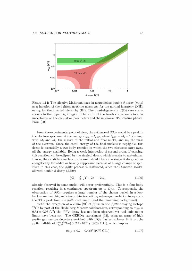
1.3. SEARCH FOR NEUTRINO MASS 43
IH HDm2<0L
NH HDm2>0L
10-4 0.001 0.01 0.1 110-4
0.001
0.01
0.1
1
m lightest @eVD
mΒ
Β@eV
D
Figure 1.14: The effective Majorana mass in neutrinoless double β decay (mββ)as a function of the lightest neutrino mass: m1 for the normal hierarchy (NH);or m3 for the inverted hierarchy (IH). The quasi-degenerate (QD) case corre-sponds to the upper right region. The width of the bands corresponds to a 3σuncertainty on the oscillation parameters and the unknown CP-violating phases.From [90].
From the experimental point of view, the evidence of ββ0ν would be a peak inthe electron spectrum at the energy Tmax = Qββ , where Qββ = Mi−Mf −2me,with Mi and Mf the masses of the initial and final nuclei, and me the massof the electron. Since the recoil energy of the final nucleus is negligible, thisdecay is essentially a two-body reaction in which the two electrons carry awayall the energy available. Being a weak interaction of second order, if existing,this reaction will be eclipsed by the single β decay, which is easier to materialize.Hence, the candidate nucleus to be used should have the single β decay eitherenergetically forbidden or heavily suppressed because of a large change of spin.Even in this case, the ββ0ν process is disfavored, since the Standard-Model-allowed double β decay (ββ2ν)
AZ X→ A
Z+2Y + 2e− + 2νe, (1.96)
already observed in some nuclei, will occur preferentially. This is a four-bodyreaction, resulting in a continuous spectrum up to Qββ . Consequently, theobservation of ββ0ν requires a large number of the chosen nuclei, in a low-background and high-efficiency detector, with good energy resolution to separatethe ββ0ν peak from the ββ2ν continuum (and the remaining background).
With the exception of a claim [91] of ββ0ν in the ββ2ν-decaying isotope76Ge by part of the Heidelberg-Moscow collaboration, corresponding to mββ =0.32 ± 0.03 eV2; the ββ0ν decay has not been observed yet and only upperlimits have been set. The GERDA experiment [92], using an array of highpurity germanium detectors enriched with 76Ge has set a lower limit on theββ0ν half-life of T 0ν
1/2(76Ge) > 2.1 · 1025 y (90% C.L.), which implies
mββ < 0.2− 0.4 eV (90% C.L.) (1.97)
44 CHAPTER 1. NEUTRINO PHYSICS
depending on the nuclear matrix element calculation.The EXO-200 experiment using a time projection chamber filled with liq-
uid xenon enriched with the ββ2ν-decaying 136Xe has set a lower limit onT 0ν
1/2(136Xe) > 1.6 · 1025 y (90% C.L.) [93] 8. Another 136Xe-based experiment,KamLAND-Zen, in which the KamLAND detector introduced in section 1.2.1 isused to look for the ββ0ν, has established the lower limit T 0ν
1/2(136Xe) > 1.9·1025
y (90% C.L.) [95]. When the EXO-200 and KamLAND-Zen limits are combined,the lower limit increases to T 0ν
1/2(136Xe) > 3.4 · 1025 y (90% C.L.), which corre-sponds to
mββ < 0.12− 0.25 eV (90% C.L.). (1.98)
More upper limits on mββ for other ββ2ν-decaying nuclei exist, but they areless stringent.
The current generation of ββ0ν experiments has the potential to reachmββ ∼ 0.1 eV. However, in order to explore the inverted hierarchy regime(cf. figure 1.14), larger experiments will be needed in the future.
1.3.3 Cosmology bounds
As the rest of the elementary particles, neutrinos were created in the firststages of the Universe after the Big Bang. Therefore, the evolution of theUniverse is sensitive to the neutrino properties, which leave an imprint on thecosmic microwave background (CMB), the large-scale structure of the Universeor the element abundances from the primordial nucleosynthesis. A detaileddiscussion of this measurements is out of the scope of this thesis, so only theconclusions regarding the neutrinos are highlighted. The cosmological datais very well described by a minimal model (the Λ Cold Dark Matter model,abbreviated ΛCDM) which assumes 3 active neutrinos with normal hierarchyand a total mass
∑mi = 0.06 eV, where mi are the masses of the neutrino mass
eigenstates, with m1 ≈ m2 ≈ 0 and m3 ≈ 0.06 eV.However, the cosmological data can be used to test extensions of the model.
From the latest CMB maps from the Planck satellite [96] and references therein,assuming 3 degenerate massive neutrinos, bounds ranging from
∑mi < 0.17−
0.72 eV (95% C.L.) are obtained depending on the data considered, with a con-servative
∑imi < 0.23 eV (95% C.L.). This result disfavors the neutrinoless
double β decay in the quasi-degenerate region with mlightest & 0.2 eV in figure1.14; and is comparable to the expected limit achievable by KATRIN on mβ .Nevertheless, the cosmology bounds are model dependent; hence, the indepen-dent information brought by a direct experiment is always valuable. In anycase, the data supports the idea of light neutrinos, which are too light to be theprimary component of the dark matter.
The cosmological data is also sensitive to the effective number of relativisticdegrees of freedom beyond the photons, Neff , during the radiation-dominatedera. In the ΛCDM model, Neff = 3.046 because of the 3 neutrinos of theStandard Model (and the corrections due to their partial decoupling during theelectron-positron annihilation phase) [96, 97]. The fit to the data results in3.04±0.18, in good agreement with the prediction, and disfavors any additionalcontribution from light particles (e.g. light sterile neutrinos). If both Neff and
8The latest analysis with increased statistics sets the lower limit on T 0ν1/2
(136Xe) > 1.1·1025
y (90% C.L.), consistent with the statistical fluctuation in the data [94].
1.4. OPEN QUESTIONS IN NEUTRINO OSCILLATIONS 45
∑imi are fitted simultaneously, consistent results are obtained: Neff = 3.2±0.5
and∑imi < 0.32 eV (both at 95% C.L.).
1.4 Open questions in neutrino oscillations
In addition to the underway experimental effort to measure the mass of theneutrinos and determine their Dirac or Majorana nature, the field of neutrinooscillations is still active and poses questions that remain unanswered.
Table 1.5 and figure 1.15 summarize the current knowledge obtained from aglobal fit to the data from the experiments presented in section 1.2.
The two most prominent challenges are determining if there is CP violationin the neutrino sector, and if positive, what is the value of the CP-violating phaseδ (cf. right middle panel in figure 1.15); and resolve the neutrino mass hierarchy,that is, what is the lightest neutrino mass eigenstate: ν1 or ν3. Both questionscan be answered measuring precisely the channel
(−)ν µ →
(−)ν e with accelerator-
based experiments, since terms sensitive to the sign of ∆m232, due to the matter
effects, and the value of δ appear in the transition probability (equation 1.68).As it was discussed in section 1.2.3, the recently measured θ13 enters also thetransition probability. Therefore, the precision in the knowledge of the θ13
mixing angle is crucial to address these questions; and reactor antineutrinoexperiments like Double Chooz provide a degeneracy-free measurement to beused as input.
If the baseline is long enough, the matter effects result in an enhancement ofthe conversion (see the resonance in equation 1.23) of neutrinos if the hierarchy isnormal (∆m2
32 > 0), or for antineutrinos if the hierarchy is inverted ∆m232 < 0.
This a consequence of Earth not being CP symmetric (it is made of matter,not antimatter), so matter effects induce a CP violation background that mustbe handled with care when measuring δ. Therefore, the determination of theneutrino mass hierarchy affects the sensitivity of the long-baseline oscillationexperiments searching for CP violation because of the degeneracy between δand sign(∆m2
32).The new NOνA experiment [100], with a baseline of ∼ 810 km might be able
to shed some light on both δ and the hierarchy. The current T2K experimenthas not a baseline long enough to contribute to the mass hierarchy research,but it has already probed some of the possible δ values. An updgrade of theSuper-Kamiokande detector to a 25-times bigger detector (Hyper-Kamiokande[101]) would increase its potential to measure δ. However, in order to studythe mass hierarchy precisely, an experiment with a longer baseline (to increasematter effects) will be needed. The DUNE experiment (formerly LBNE [102]),currently in the design phase, with a long baseline (∼ 1300 km) and an intensebeam with a broad energy spectrum (peaked at ∼ 2.5 GeV) might answer bothδ and sign(∆m2
32) questions.The mass hierarchy can also be resolved using non-accelerator experiments.
The disappearance of atmospheric muon neutrinos is also sensitive to the mattereffects, and huge baselines are available from the study of the neutrinos crossingthe Earth. Future experiments using large masses of water, either frozen as theAntarctic ice (IceCUBE-PINGU [103]) or liquid as in the Mediterranean sea(KM3Net-ORCA [104]) or confined in a volume (Hyper-Kamiokande), as waterCherenkov detectors will be able to compete in the search. Other large detectors
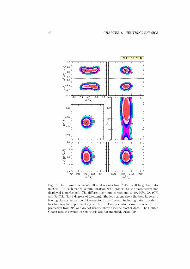
46 CHAPTER 1. NEUTRINO PHYSICS
0.2 0.25 0.3 0.35 0.4
sin2
θ12
6.5
7
7.5
8
8.5
∆m
2 21 [
10
-5 e
V2]
0.015 0.02 0.025 0.03
sin2
θ13
0.015
0.02
0.025
0.03
sin
2θ
13
0
90
180
270
360
δC
P
0.3 0.4 0.5 0.6 0.7
sin2
θ23
-2.8
-2.6
-2.4
-2.2
2.2
2.4
2.6
2.8
∆m
2 32
[1
0-3
eV
2]
∆
m2 31
NuFIT 2.0 (2014)
Figure 1.15: Two-dimensional allowed regions from NuFit 2.0 to global datain 2014. In each panel, a minimization with respect to the parameters notdisplayed is performed. The different contours correspond to 1σ, 90%, 2σ, 99%and 3σ C.L. (for 2 degrees of freedom). Shaded regions show the best fit resultsleaving the normalization of the reactor fluxes free and including data from shortbaseline reactor experiments (L < 100 m). Empty contours use the reactor fluxprediction from [98] and do not use the short baseline reactor data. The DoubleChooz results covered in this thesis are not included. From [99].
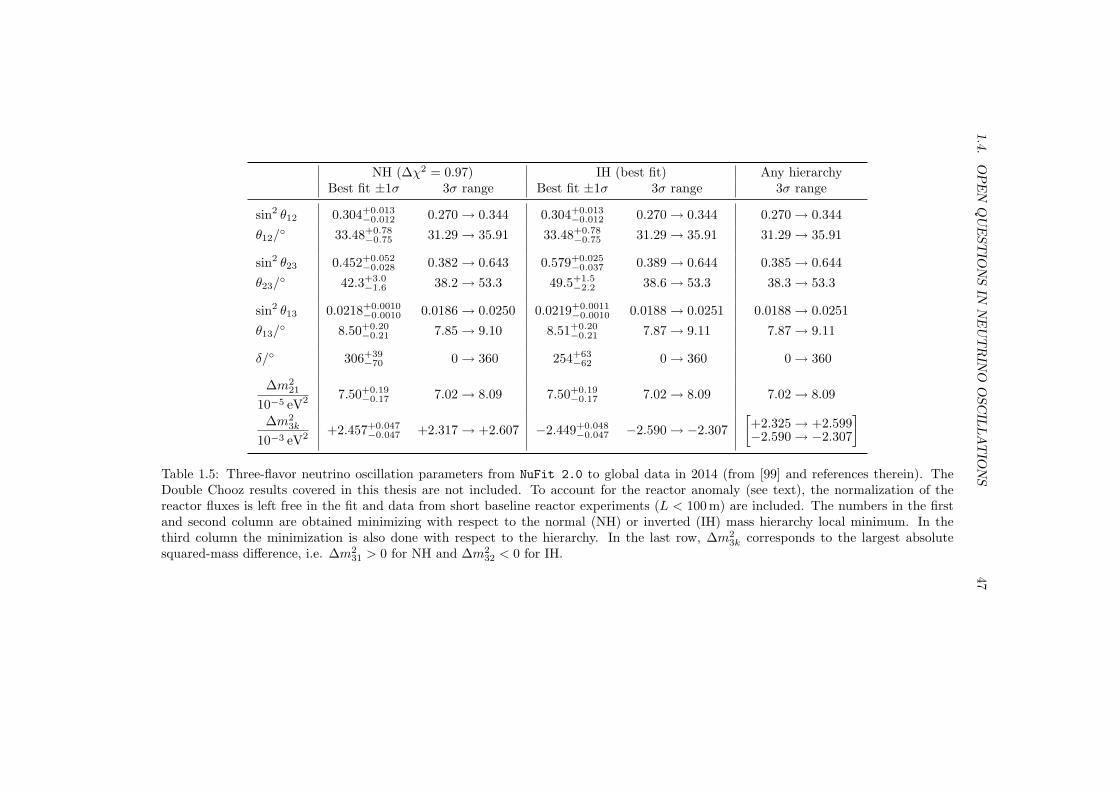
1.4.O
PE
NQ
UE
ST
ION
SIN
NE
UT
RIN
OO
SC
ILLA
TIO
NS
47
NH (∆χ2 = 0.97) IH (best fit) Any hierarchyBest fit ±1σ 3σ range Best fit ±1σ 3σ range 3σ range
sin2 θ12 0.304+0.013−0.012 0.270→ 0.344 0.304+0.013
−0.012 0.270→ 0.344 0.270→ 0.344θ12/
33.48+0.78−0.75 31.29→ 35.91 33.48+0.78
−0.75 31.29→ 35.91 31.29→ 35.91
sin2 θ23 0.452+0.052−0.028 0.382→ 0.643 0.579+0.025
−0.037 0.389→ 0.644 0.385→ 0.644θ23/
42.3+3.0−1.6 38.2→ 53.3 49.5+1.5
−2.2 38.6→ 53.3 38.3→ 53.3
sin2 θ13 0.0218+0.0010−0.0010 0.0186→ 0.0250 0.0219+0.0011
−0.0010 0.0188→ 0.0251 0.0188→ 0.0251θ13/
8.50+0.20−0.21 7.85→ 9.10 8.51+0.20
−0.21 7.87→ 9.11 7.87→ 9.11
δ/ 306+39−70 0→ 360 254+63
−62 0→ 360 0→ 360
∆m221
10−5 eV2 7.50+0.19−0.17 7.02→ 8.09 7.50+0.19
−0.17 7.02→ 8.09 7.02→ 8.09
∆m23k
10−3 eV2 +2.457+0.047−0.047 +2.317→ +2.607 −2.449+0.048
−0.047 −2.590→ −2.307[+2.325→ +2.599−2.590→ −2.307
]
Table 1.5: Three-flavor neutrino oscillation parameters from NuFit 2.0 to global data in 2014 (from [99] and references therein). TheDouble Chooz results covered in this thesis are not included. To account for the reactor anomaly (see text), the normalization of thereactor fluxes is left free in the fit and data from short baseline reactor experiments (L < 100 m) are included. The numbers in the firstand second column are obtained minimizing with respect to the normal (NH) or inverted (IH) mass hierarchy local minimum. In thethird column the minimization is also done with respect to the hierarchy. In the last row, ∆m2
3k corresponds to the largest absolutesquared-mass difference, i.e. ∆m2
31 > 0 for NH and ∆m232 < 0 for IH.
48 CHAPTER 1. NEUTRINO PHYSICS
such as magnetized iron calorimeters (ICAL [105]), or the liquid argon timeprojection chamber acting as the far detector in DUNE might profit also fromthe atmospheric neutrinos channel. The disappearance of electron antineutrinosfrom reactors at the first minimum due to (∆m2
21, θ12), equal to a distance of∼ 50 km, is also sensitive to the mass hierarchy from the interplay between theterms containing ∆m2
32 and ∆m231 in equation 1.53. In order to observe this
effect, a detailed knowledge of the reactor antineutrino spectrum is necessaryand an excellent energy resolution is required. The JUNO experiment [106] willpursue this measurement.
Currently, it is known that θ23 is close to π/4 (or 45, see table 1.5), butit is not known whether it lies in the first octant (θ23 < π/4), in the second(θ23 > π/4) or it is just the maximal mixing (between the ν2 and ν3 masseigenstates) value θ23 = π/4 (cf. upper left panel in figure 1.15). The precisestudy of the channels
(−)ν µ →
(−)ν e and
(−)ν µ →
(−)ν µ with the aforementioned
detectors has the potential to discriminate between the different options. Thedetermination of the actual value of θ23 is important, not only because it impactsthe sensitivity of the future experiments that will measure the mass hierarchyand the CP violation, but also because it can point to flavor symmetries toexplain the structure of the PMNS matrix,
|UPMNS| ∼
0.8 0.5 0.20.5 0.6 0.60.2 0.6 0.8
, (1.99)
and why it is so different from the almost-diagonal CKM matrix in the quarksector,
|VCKM| ≈
1 0.2 0.0040.2 1 0.04
0.009 0.04 1
. (1.100)
As it has been described in this chapter, the three-flavor neutrino frame-work describes successfully almost all the experimental data available. However,some experiments have obtained results which cannot be accommodated in thisframework.
A long-standing anomaly is that initiated by the excess of νe events in theLSND experiment. The LSND experiment ran between 1993 and 1998 at LosAlamos National Laboratory (New Mexico, USA). LSND used a νµ beam gen-erated from decay-at-rest pions directed towards a liquid scintillator detector30 m downstream, and looked for the appearance of νe via inverse-β decay oncarbon nuclei. A final excess of 87.9± 22.4± 6 of νe events above backgroundsin the positron energy range between 20 MeV and 60 MeV was reported [107].If interpreted as a result of oscillations, it points to a squared-mass difference inthe range ∆m2 = 0.2−10 eV2. This squared-mass difference is much larger than∆m2
21 or ∆m232, suggesting the existence of a new mass eigenstate heavier than
the known ones. This mass eigenstate would require a new state in the flavorbasis, which must be sterile in order to escape the constrain imposed by the Zboson width explained in section 1.1. However, the KARMEN experiment, withsimilar beam and detector distance did not observe any excess [108], althoughit could not exclude completely the LSND result (see figure 1.16).
The LSND anomaly was further investigated by the MiniBooNE experimentat the Fermi National Accelerator Laboratory using both νµ and νµ beams
1.4. OPEN QUESTIONS IN NEUTRINO OSCILLATIONS 49
created from the decay in flight of pions. The beams had a wide energy distri-bution, peaked at 400 MeV for νµ and 600 MeV for νµ, and a low contaminationof electron-flavor (anti)neutrinos (≤ 0.5%). The detector was placed at a dis-tance of ∼ 540 m from the production point, so it could explore a similar L/Eregion as LSND. The detector was a mineral-oil Cherenkov detector, in whichthe flavor of the neutrino was revealed from the Cherenkov light emitted bythe charged lepton produced upon charged-current interaction. MiniBooNEobserved excesses in both antineutrino and neutrino modes in the neutrino en-ergy interval (200, 1250) MeV [109]. The antineutrino excess, 78.4± 28.5 events(2.8σ), when interpreted as oscillation-induced, gives an allowed parameter re-gion which overlaps partially with the LSND one (cf. figure 1.16). On the otherhand, the neutrino excess, 162.0 ± 47.8 events (3.4σ), is concentrated at lowenergy, where is barely compatible with an oscillation interpretation.
It is important to remark that the MiniBooNE detector cannot distinguishbetween electrons and γ-rays. For that reason, MicroBooNE [110], a new ex-periment in the same beamline as MiniBooNE has been built, in which a liquidargon time projection chamber (LArTPC) will be used as detector at ∼ 470 mfrom the production point. The excellent tracking and calorimetric capabilitiesof the LArTPC allow to tell the electrons from γ-rays, addressing the natureof the excess. Furthermore, adding SBND (formerly LAr1-ND [111]), a neardetector at ∼ 100 m from the beam production point, will reduce the system-atic uncertainties affecting the oscillation search, enhancing the sensitivity inthe electron-flavor appearance and muon-flavor disappearance charged-currentdetection channels, and opening the possibility to look for disappearance of ac-tive neutrinos into sterile neutrinos using neutral-current interactions. Finally,the LSND allowed region will be completely explored with the addition of thelarge ICARUS T600 LArTPC detector at ∼ 600 m, which is moving from GranSasso to the Fermi National Accelerator Laboratory with an overhauling stopat CERN [112].
Another anomaly, the gallium anomaly [113], has arisen from the reanalysisof the calibration data in the GALLEX/GNO and SAGE solar neutrino radio-chemical detectors (introduced in section 1.2.1). These detectors used 51Cr and37Ar (only SAGE) sources, which decay via electron capture emitting monochro-matic νe with energies below 1 MeV, to measure their efficiency to detect solarneutrinos using the reaction in equation 1.29. The combination of four calibra-tion runs, two at each detector, gives an observed-to-expected ratio of
RGa = 0.76+0.09−0.08, (1.101)
which is 3σ away from 1. If the result is interpreted as a consequence of νedisappearance due to oscillation into an undetectable flavor in a two-neutrinoapproximation, it is found sin2(2θ) & 0.07 and ∆m2 & 0.35 eV2 at 99% C.L.
Moreover, the reevaluation of the reactor antineutrino fluxes to be usedby the current θ13 experiments resulted in a normalization shift of +3% [114,98] (the Double Chooz prediction is explained in section 2.4.1). When thedata from past reactor experiments performed at short baselines (< 100 m) isreanalyzed with the new flux prediction, an overall deficit appears in the ratioof the observed to predicted νe events:
RSBL = 0.943± 0.023. (1.102)
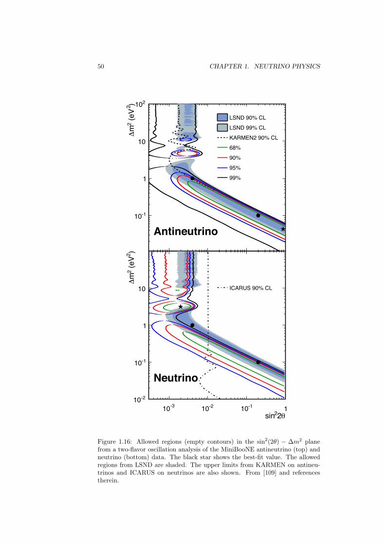
50 CHAPTER 1. NEUTRINO PHYSICS
)2 (e
V2
m
-110
1
10
210
LSND 90% CLLSND 99% CLKARMEN2 90% CL68%90%95%99%
Antineutrino
22sin-310 -210 -110 1
)2 (e
V2
m
-210
-110
1
10 ICARUS 90% CL
Neutrino
Figure 1.16: Allowed regions (empty contours) in the sin2(2θ) − ∆m2 planefrom a two-flavor oscillation analysis of the MiniBooNE antineutrino (top) andneutrino (bottom) data. The black star shows the best-fit value. The allowedregions from LSND are shaded. The upper limits from KARMEN on antineu-trinos and ICARUS on neutrinos are also shown. From [109] and referencestherein.
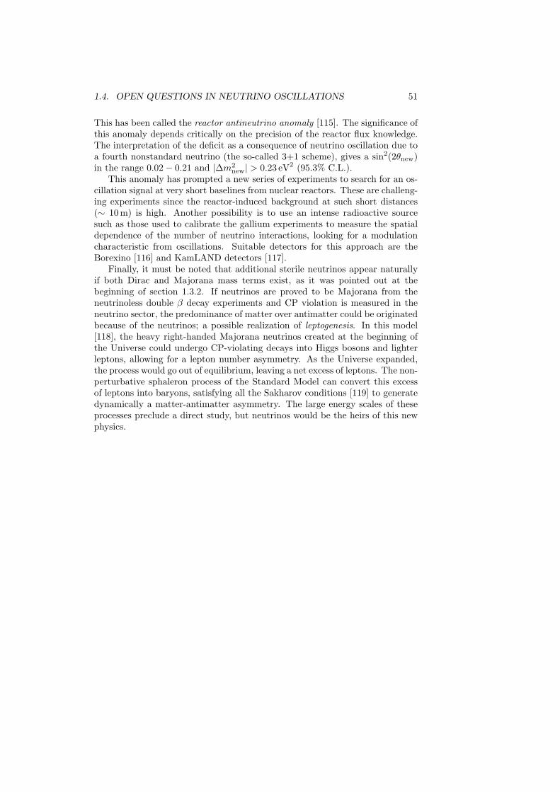
1.4. OPEN QUESTIONS IN NEUTRINO OSCILLATIONS 51
This has been called the reactor antineutrino anomaly [115]. The significance ofthis anomaly depends critically on the precision of the reactor flux knowledge.The interpretation of the deficit as a consequence of neutrino oscillation due toa fourth nonstandard neutrino (the so-called 3+1 scheme), gives a sin2(2θnew)in the range 0.02− 0.21 and |∆m2
new| > 0.23 eV2 (95.3% C.L.).This anomaly has prompted a new series of experiments to search for an os-
cillation signal at very short baselines from nuclear reactors. These are challeng-ing experiments since the reactor-induced background at such short distances(∼ 10 m) is high. Another possibility is to use an intense radioactive sourcesuch as those used to calibrate the gallium experiments to measure the spatialdependence of the number of neutrino interactions, looking for a modulationcharacteristic from oscillations. Suitable detectors for this approach are theBorexino [116] and KamLAND detectors [117].
Finally, it must be noted that additional sterile neutrinos appear naturallyif both Dirac and Majorana mass terms exist, as it was pointed out at thebeginning of section 1.3.2. If neutrinos are proved to be Majorana from theneutrinoless double β decay experiments and CP violation is measured in theneutrino sector, the predominance of matter over antimatter could be originatedbecause of the neutrinos; a possible realization of leptogenesis. In this model[118], the heavy right-handed Majorana neutrinos created at the beginning ofthe Universe could undergo CP-violating decays into Higgs bosons and lighterleptons, allowing for a lepton number asymmetry. As the Universe expanded,the process would go out of equilibrium, leaving a net excess of leptons. The non-perturbative sphaleron process of the Standard Model can convert this excessof leptons into baryons, satisfying all the Sakharov conditions [119] to generatedynamically a matter-antimatter asymmetry. The large energy scales of theseprocesses preclude a direct study, but neutrinos would be the heirs of this newphysics.

52 CHAPTER 1. NEUTRINO PHYSICS
Chapter 2
The Double Choozexperiment
Double Chooz 1 is a two-detector experiment to measure the neutrino mix-ing angle θ13 from the oscillation-induced deficit of electron antineutrinos in theflux emitted by the nuclear reactors of the Chooz power plant. The experimentconcept and site are described in section 2.1. The detection of the electron an-tineutrinos is discussed in section 2.2 and the design of the detector is explainedin section 2.3. The Monte Carlo simulation which provides the expected numberof electron antineutrinos in the detector is described in section 2.4.
2.1 Experiment concept
The idea of a two-detector reactor experiment to search for the disappearanceof νe due to the oscillation driven by θ13 (see equation 1.54) was first proposedin [120]. The use of two detectors, one close to the reactor at a distance ofO(100 m) (the Near Detector) and one distant at O(1 km) (the Far Detector),to measure simultaneously the νe flux emitted by the reactor would allow tocancel the uncertainty in the reactor flux in the relative comparison of bothmeasurements 2. In addition, by building the two detectors as identical aspossible, the systematic uncertainty in the νe detection could be canceled aswell, except for the uncorrelated part accounting for the remaining differencesbetween the detectors, which could be minimized with thorough calibration andmonitoring. Since these two sources (reactor flux and νe detection) were thedominant systematic uncertainties affecting the best experimental limit on θ13
at the time, set by the CHOOZ experiment [63] (figure 1.11), a two-detectorexperiment was guaranteed to make a significant improvement in the knowledgeof this mixing angle.
Double Chooz [66] was originally proposed around the year 2004 as a fastand moderate-cost experiment to measure sin2(2θ13) ≥ 0.05 at 3σ or set a limitsin2(2θ13) < 0.03 at 90% C.L. after 3 years of data taking with two detectors,
1Chooz is pronounced as “sho”.2The magnitude of the cancellation of the uncertainty in the νe flux when two or more
reactor cores are present depends on the location of the detectors with respect to the reactors.This is further discussed at the end of the section.
53
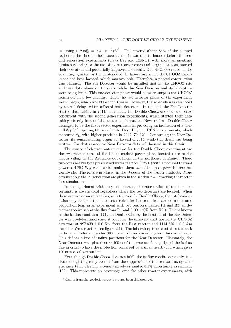
54 CHAPTER 2. THE DOUBLE CHOOZ EXPERIMENT
assuming a ∆m231 = 2.4 · 10−3 eV2. This covered about 85% of the allowed
region at the time of the proposal, and it was due to happen before the sec-ond generation experiments (Daya Bay and RENO), with more antineutrinoluminosity owing to the use of more reactor cores and larger detectors, startedtheir operation and potentially improved the result. Double Chooz relied on theadvantage granted by the existence of the laboratory where the CHOOZ exper-iment had been located, which was available. Therefore, a phased constructionwas planned. The Far Detector would be installed first in the CHOOZ siteand take data alone for 1.5 years, while the Near Detector and its laboratorywere being built. This one-detector phase would allow to surpass the CHOOZsensitivity in a few months. Then the two-detector phase of the experimentwould begin, which would last for 3 years. However, the schedule was disruptedby several delays which affected both detectors. In the end, the Far Detectorstarted data taking in 2011. This made the Double Chooz one-detector phaseconcurrent with the second generation experiments, which started their datataking directly in a multi-detector configuration. Nevertheless, Double Choozmanaged to be the first reactor experiment in providing an indication of a non-null θ13 [69], opening the way for the Daya Bay and RENO experiments, whichmeasured θ13 with higher precision in 2012 [70, 121]. Concerning the Near De-tector, its commissioning began at the end of 2014, while this thesis was beingwritten. For that reason, no Near Detector data will be used in this thesis.
The source of electron antineutrinos for the Double Chooz experiment arethe two reactor cores of the Chooz nuclear power plant, located close to theChooz village in the Ardennes department in the northeast of France. Thesetwo cores are N4 type pressurized water reactors (PWR) with a nominal thermalpower of 4.25 GWth each, which makes them two of the most powerful reactorsworldwide. The νe are produced in the β-decay of the fission products. Moredetails about the νe generation are given in the section 2.4.1 covering the reactorflux simulation.
In an experiment with only one reactor, the cancellation of the flux un-certainty is always total regardless where the two detectors are located. Whenthere are two or more reactors, as is the case for Double Chooz, the total cancel-lation only occurs if the detectors receive the flux from the reactors in the sameproportion (e.g. in an experiment with two reactors, named R1 and R2, all de-tectors receive x% of the flux from R1 and (100−x)% from R2.). This is knownas the isoflux condition [122]. In Double Chooz, the location of the Far Detec-tor was predetermined since it occupies the same pit that hosted the CHOOZdetector, at 997.839 ± 0.015 m from the East reactor and 1114.656 ± 0.015 mfrom the West reactor (see figure 2.1). The laboratory is excavated in the rockunder a hill which provides 300 m.w.e. of overburden against the cosmic rays.This defines a line of isoflux positions for the Near Detector. Ultimately, theNear Detector was placed at ∼ 400 m of the reactors 3, slightly off the isofluxline in order to have the protection conferred by a small nearby hill which gives120 m.w.e. of overburden.
Even though Double Chooz does not fulfill the isoflux condition exactly, it isclose enough to greatly benefit from the suppression of the reactor flux system-atic uncertainty, leaving a conservatively estimated 0.1% uncertainty as remnant[122]. This represents an advantage over the other reactor experiments, with
3Results from the geodetic survey have not been disclosed yet.
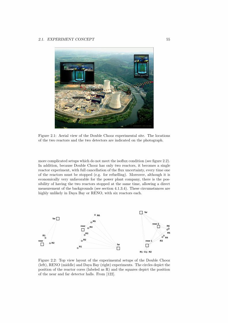
2.1. EXPERIMENT CONCEPT 55
Figure 2.1: Aerial view of the Double Chooz experimental site. The locationsof the two reactors and the two detectors are indicated on the photograph.
more complicated setups which do not meet the isoflux condition (see figure 2.2).In addition, because Double Chooz has only two reactors, it becomes a singlereactor experiment, with full cancellation of the flux uncertainty, every time oneof the reactors must be stopped (e.g. for refuelling). Moreover, although it iseconomically very unfavorable for the power plant company, there is the pos-sibility of having the two reactors stopped at the same time, allowing a directmeasurement of the backgrounds (see section 4.1.3.4). These circumstances arehighly unlikely in Daya Bay or RENO, with six reactors each.
near 1
near 2
far
R1
far
near
R2
R3
R4
R5
R6
R1
R2
R3
R4
R5
R6
far
near
R1
R2
Figure 2.2: Top view layout of the experimental setups of the Double Chooz(left), RENO (middle) and Daya Bay (right) experiments. The circles depict theposition of the reactor cores (labeled as R) and the squares depict the positionof the near and far detector halls. From [122].
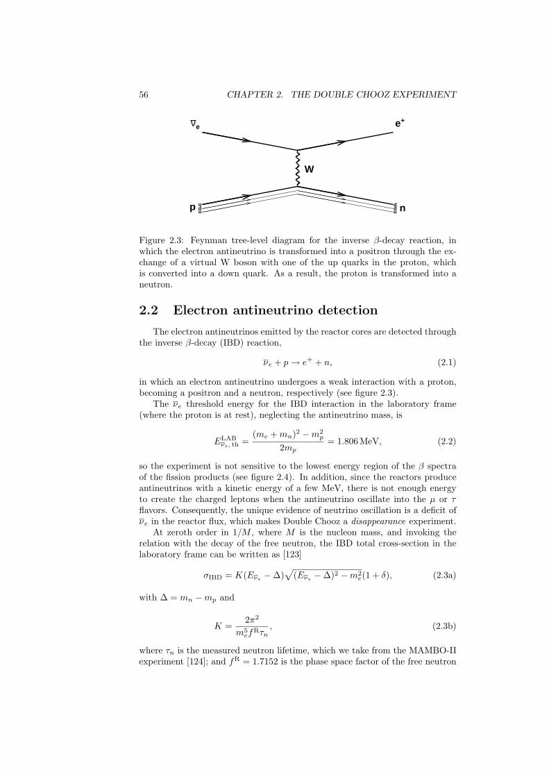
56 CHAPTER 2. THE DOUBLE CHOOZ EXPERIMENT
p udu
eν
W
nddu
+e
Figure 2.3: Feynman tree-level diagram for the inverse β-decay reaction, inwhich the electron antineutrino is transformed into a positron through the ex-change of a virtual W boson with one of the up quarks in the proton, whichis converted into a down quark. As a result, the proton is transformed into aneutron.
2.2 Electron antineutrino detection
The electron antineutrinos emitted by the reactor cores are detected throughthe inverse β-decay (IBD) reaction,
νe + p→ e+ + n, (2.1)
in which an electron antineutrino undergoes a weak interaction with a proton,becoming a positron and a neutron, respectively (see figure 2.3).
The νe threshold energy for the IBD interaction in the laboratory frame(where the proton is at rest), neglecting the antineutrino mass, is
ELABνe, th =
(me +mn)2 −m2p
2mp= 1.806 MeV, (2.2)
so the experiment is not sensitive to the lowest energy region of the β spectraof the fission products (see figure 2.4). In addition, since the reactors produceantineutrinos with a kinetic energy of a few MeV, there is not enough energyto create the charged leptons when the antineutrino oscillate into the µ or τflavors. Consequently, the unique evidence of neutrino oscillation is a deficit ofνe in the reactor flux, which makes Double Chooz a disappearance experiment.
At zeroth order in 1/M , where M is the nucleon mass, and invoking therelation with the decay of the free neutron, the IBD total cross-section in thelaboratory frame can be written as [123]
σIBD = K(Eνe −∆)√
(Eνe −∆)2 −m2e(1 + δ), (2.3a)
with ∆ = mn −mp and
K =2π2
m5ef
Rτn, (2.3b)
where τn is the measured neutron lifetime, which we take from the MAMBO-IIexperiment [124]; and fR = 1.7152 is the phase space factor of the free neutron
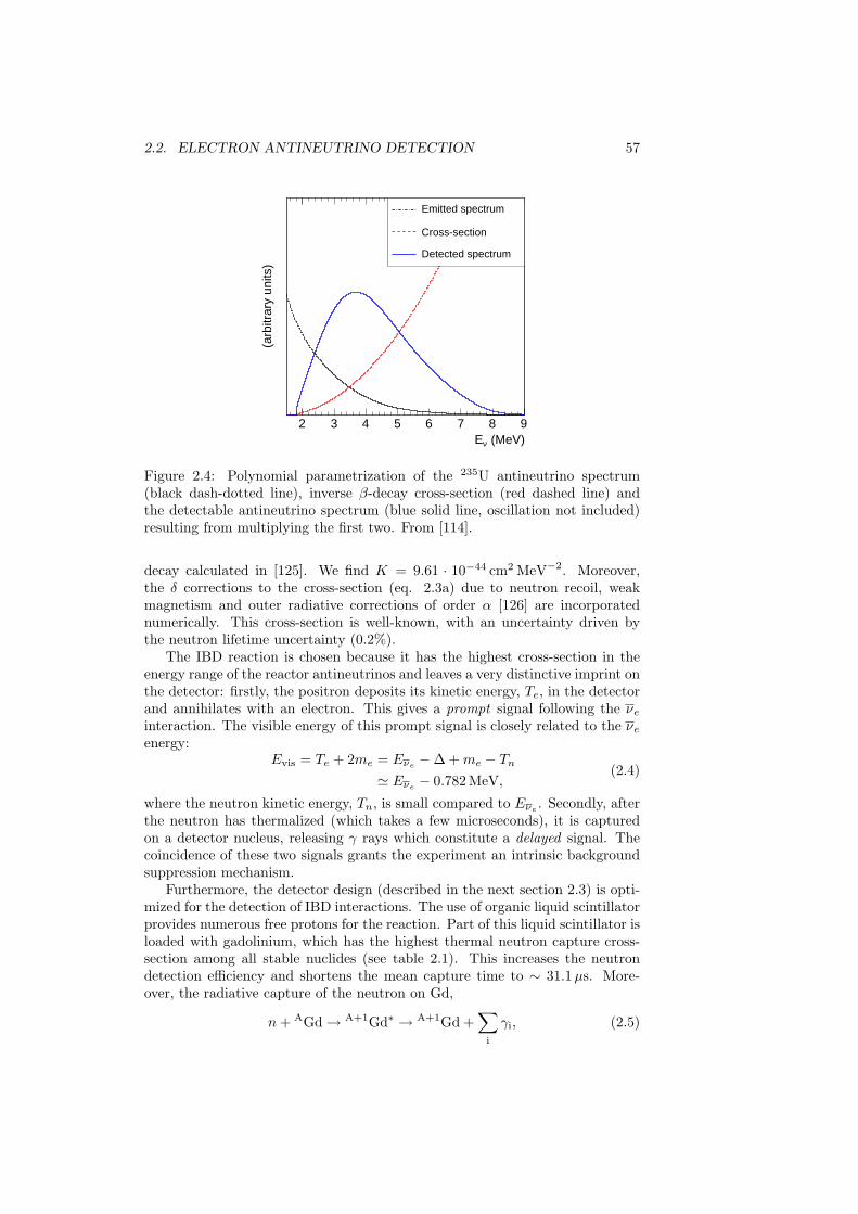
2.2. ELECTRON ANTINEUTRINO DETECTION 57
(MeV)νE2 3 4 5 6 7 8 9
(arb
itrar
y un
its)
Emitted spectrum
Cross-section
Detected spectrum
Figure 2.4: Polynomial parametrization of the 235U antineutrino spectrum(black dash-dotted line), inverse β-decay cross-section (red dashed line) andthe detectable antineutrino spectrum (blue solid line, oscillation not included)resulting from multiplying the first two. From [114].
decay calculated in [125]. We find K = 9.61 · 10−44 cm2 MeV−2. Moreover,the δ corrections to the cross-section (eq. 2.3a) due to neutron recoil, weakmagnetism and outer radiative corrections of order α [126] are incorporatednumerically. This cross-section is well-known, with an uncertainty driven bythe neutron lifetime uncertainty (0.2%).
The IBD reaction is chosen because it has the highest cross-section in theenergy range of the reactor antineutrinos and leaves a very distinctive imprint onthe detector: firstly, the positron deposits its kinetic energy, Te, in the detectorand annihilates with an electron. This gives a prompt signal following the νeinteraction. The visible energy of this prompt signal is closely related to the νeenergy:
Evis = Te + 2me = Eνe −∆ +me − Tn' Eνe − 0.782 MeV,
(2.4)
where the neutron kinetic energy, Tn, is small compared to Eνe . Secondly, afterthe neutron has thermalized (which takes a few microseconds), it is capturedon a detector nucleus, releasing γ rays which constitute a delayed signal. Thecoincidence of these two signals grants the experiment an intrinsic backgroundsuppression mechanism.
Furthermore, the detector design (described in the next section 2.3) is opti-mized for the detection of IBD interactions. The use of organic liquid scintillatorprovides numerous free protons for the reaction. Part of this liquid scintillator isloaded with gadolinium, which has the highest thermal neutron capture cross-section among all stable nuclides (see table 2.1). This increases the neutrondetection efficiency and shortens the mean capture time to ∼ 31.1µs. More-over, the radiative capture of the neutron on Gd,
n+ AGd→ A+1Gd∗ → A+1Gd +∑
i
γi, (2.5)
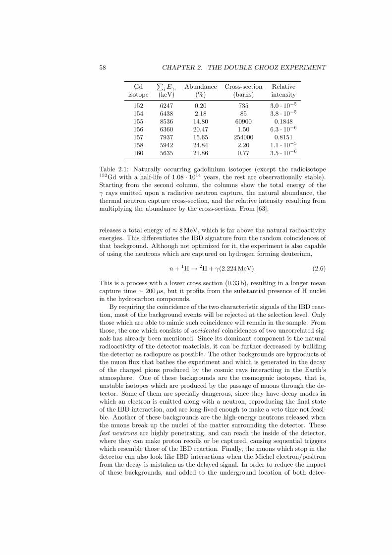
58 CHAPTER 2. THE DOUBLE CHOOZ EXPERIMENT
Gd∑iEγi Abundance Cross-section Relative
isotope (keV) (%) (barns) intensity
152 6247 0.20 735 3.0 · 10−5
154 6438 2.18 85 3.8 · 10−5
155 8536 14.80 60900 0.1848156 6360 20.47 1.50 6.3 · 10−6
157 7937 15.65 254000 0.8151158 5942 24.84 2.20 1.1 · 10−5
160 5635 21.86 0.77 3.5 · 10−6
Table 2.1: Naturally occurring gadolinium isotopes (except the radioisotope152Gd with a half-life of 1.08 · 1014 years, the rest are observationally stable).Starting from the second column, the columns show the total energy of theγ rays emitted upon a radiative neutron capture, the natural abundance, thethermal neutron capture cross-section, and the relative intensity resulting frommultiplying the abundance by the cross-section. From [63].
releases a total energy of ≈ 8 MeV, which is far above the natural radioactivityenergies. This differentiates the IBD signature from the random coincidences ofthat background. Although not optimized for it, the experiment is also capableof using the neutrons which are captured on hydrogen forming deuterium,
n+ 1H→ 2H + γ(2.224 MeV). (2.6)
This is a process with a lower cross section (0.33 b), resulting in a longer meancapture time ∼ 200µs, but it profits from the substantial presence of H nucleiin the hydrocarbon compounds.
By requiring the coincidence of the two characteristic signals of the IBD reac-tion, most of the background events will be rejected at the selection level. Onlythose which are able to mimic such coincidence will remain in the sample. Fromthose, the one which consists of accidental coincidences of two uncorrelated sig-nals has already been mentioned. Since its dominant component is the naturalradioactivity of the detector materials, it can be further decreased by buildingthe detector as radiopure as possible. The other backgrounds are byproducts ofthe muon flux that bathes the experiment and which is generated in the decayof the charged pions produced by the cosmic rays interacting in the Earth’satmosphere. One of these backgrounds are the cosmogenic isotopes, that is,unstable isotopes which are produced by the passage of muons through the de-tector. Some of them are specially dangerous, since they have decay modes inwhich an electron is emitted along with a neutron, reproducing the final stateof the IBD interaction, and are long-lived enough to make a veto time not feasi-ble. Another of these backgrounds are the high-energy neutrons released whenthe muons break up the nuclei of the matter surrounding the detector. Thesefast neutrons are highly penetrating, and can reach the inside of the detector,where they can make proton recoils or be captured, causing sequential triggerswhich resemble those of the IBD reaction. Finally, the muons which stop in thedetector can also look like IBD interactions when the Michel electron/positronfrom the decay is mistaken as the delayed signal. In order to reduce the impactof these backgrounds, and added to the underground location of both detec-
2.3. DETECTOR DESIGN 59
tors, the detector includes several active subdetectors which are described inthe next section. These backgrounds and how the active subdetectors are usedto reject most of their contribution are explained in detail in sections 4.1.3 (forthe Gd-based νe selection) and 4.2.3 (for the H-based νe selection).
2.3 Detector design
The Double Chooz detector consists of a cylindrical main detector, enclosedby shielding and covered by an outer veto. The main detector is formed by fourconcentric cylindrical volumes (called Target, Gamma Catcher, Buffer and InnerVeto) which are nested in the fashion of a matryoshka doll (see figure 2.5). Inorder to avoid mechanical stress on the vessels, the liquids which fill each volumehave their densities matched to 0.804± 0.001 g/cm3 at 15 C, which is close tothe detector mean temperature.
The detector can be conceptually divided into two big subdetectors by con-sidering the kind of events they are designed for: an Inner Detector for measur-ing the signal events, and an Outer Detector to act as a background veto.
2.3.1 Inner Detector
The Inner Detector is the part of the detector aimed to measure the signalsproduced by the IBD interaction of the νe. It is a liquid scintillator calorimeterwhich is divided into three concentrical cylindrical volumes: the Target, theGamma Catcher and the Buffer. A central chimney, connected to the threevolumes, was used to fill them. It is observed by 390 low background 10-inchphotomultiplier tubes (PMT) (Hamamatsu R7081) installed on the inner wallsof the Buffer.
Target
The innermost volume, the Target, is an 8 mm thick acrylic vessel (radius1150 mm, height 2458 mm), transparent to UV to visible light, filled with 10.3 m3
of liquid scintillator loaded with Gd to enhance the capture of the IBD neu-trons. The scintillator solvent consists of o-PXE (ortho-phenylxylylethane) andn-dodecane, in a volume concentration of 20% and 80%, respectively. Two addi-tional fluors are added, PPO (2,5-diphenyloxazole) as the primary fluor (7 g/l),and bis-MSB (1,4-bis-(2-methylstyryl)benzene) as second wavelength shifter (20mg/l), in order to shift the scintillation light to a region in which the mixtureis more transparent and the PMTs have the highest quantum efficiency.
The gadolinium metal does not dissolve well in the organic liquids whichmake up the scintillator. This can cause problems in the optical stability ofthe scintillator, as it happened in the CHOOZ experiment [63]. In order toachieve a higher solubility and a durable chemical stability, a metalorganic com-plex is used, Gd(thd)3 (Gd(III)-tris-(2,2,6,6-tetramethyl-heptane-3,5-dionate)),a metal-β-diketone [127]. These complexes have a high vapor pressure, whichmakes possible to purify them by sublimation, thus reducing the radioactivecontamination of K, U and Th. The Gd concentration (0.123% by weight, cor-responding approximately to 1 g/l) is chosen as a compromise between a high
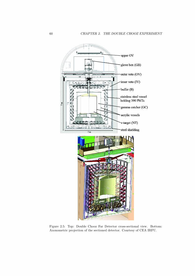
60 CHAPTER 2. THE DOUBLE CHOOZ EXPERIMENT
Figure 2.5: Top: Double Chooz Far Detector cross-sectional view. Bottom:Axonometric projection of the sectioned detector. Courtesy of CEA IRFU.
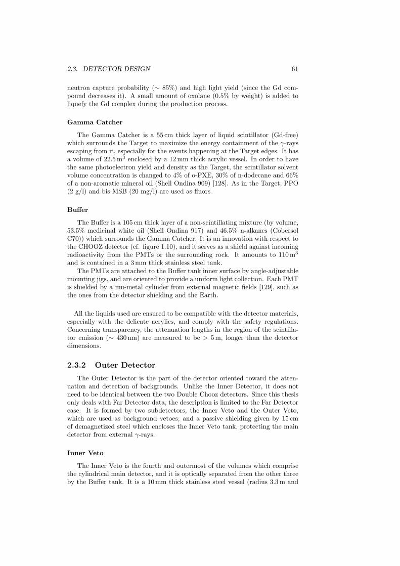
2.3. DETECTOR DESIGN 61
neutron capture probability (∼ 85%) and high light yield (since the Gd com-pound decreases it). A small amount of oxolane (0.5% by weight) is added toliquefy the Gd complex during the production process.
Gamma Catcher
The Gamma Catcher is a 55 cm thick layer of liquid scintillator (Gd-free)which surrounds the Target to maximize the energy containment of the γ-raysescaping from it, especially for the events happening at the Target edges. It hasa volume of 22.5 m3 enclosed by a 12 mm thick acrylic vessel. In order to havethe same photoelectron yield and density as the Target, the scintillator solventvolume concentration is changed to 4% of o-PXE, 30% of n-dodecane and 66%of a non-aromatic mineral oil (Shell Ondina 909) [128]. As in the Target, PPO(2 g/l) and bis-MSB (20 mg/l) are used as fluors.
Buffer
The Buffer is a 105 cm thick layer of a non-scintillating mixture (by volume,53.5% medicinal white oil (Shell Ondina 917) and 46.5% n-alkanes (CobersolC70)) which surrounds the Gamma Catcher. It is an innovation with respect tothe CHOOZ detector (cf. figure 1.10), and it serves as a shield against incomingradioactivity from the PMTs or the surrounding rock. It amounts to 110 m3
and is contained in a 3 mm thick stainless steel tank.The PMTs are attached to the Buffer tank inner surface by angle-adjustable
mounting jigs, and are oriented to provide a uniform light collection. Each PMTis shielded by a mu-metal cylinder from external magnetic fields [129], such asthe ones from the detector shielding and the Earth.
All the liquids used are ensured to be compatible with the detector materials,especially with the delicate acrylics, and comply with the safety regulations.Concerning transparency, the attenuation lengths in the region of the scintilla-tor emission (∼ 430 nm) are measured to be > 5 m, longer than the detectordimensions.
2.3.2 Outer Detector
The Outer Detector is the part of the detector oriented toward the atten-uation and detection of backgrounds. Unlike the Inner Detector, it does notneed to be identical between the two Double Chooz detectors. Since this thesisonly deals with Far Detector data, the description is limited to the Far Detectorcase. It is formed by two subdetectors, the Inner Veto and the Outer Veto,which are used as background vetoes; and a passive shielding given by 15 cmof demagnetized steel which encloses the Inner Veto tank, protecting the maindetector from external γ-rays.
Inner Veto
The Inner Veto is the fourth and outermost of the volumes which comprisethe cylindrical main detector, and it is optically separated from the other threeby the Buffer tank. It is a 10 mm thick stainless steel vessel (radius 3.3 m and
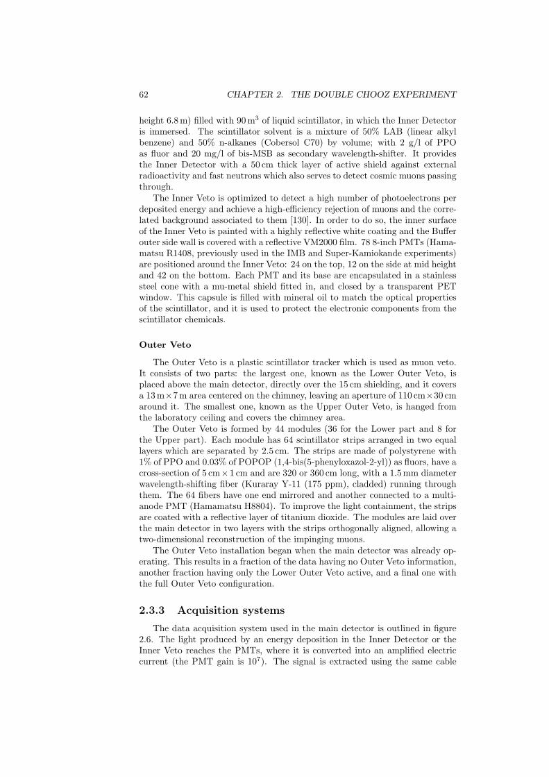
62 CHAPTER 2. THE DOUBLE CHOOZ EXPERIMENT
height 6.8 m) filled with 90 m3 of liquid scintillator, in which the Inner Detectoris immersed. The scintillator solvent is a mixture of 50% LAB (linear alkylbenzene) and 50% n-alkanes (Cobersol C70) by volume; with 2 g/l of PPOas fluor and 20 mg/l of bis-MSB as secondary wavelength-shifter. It providesthe Inner Detector with a 50 cm thick layer of active shield against externalradioactivity and fast neutrons which also serves to detect cosmic muons passingthrough.
The Inner Veto is optimized to detect a high number of photoelectrons perdeposited energy and achieve a high-efficiency rejection of muons and the corre-lated background associated to them [130]. In order to do so, the inner surfaceof the Inner Veto is painted with a highly reflective white coating and the Bufferouter side wall is covered with a reflective VM2000 film. 78 8-inch PMTs (Hama-matsu R1408, previously used in the IMB and Super-Kamiokande experiments)are positioned around the Inner Veto: 24 on the top, 12 on the side at mid heightand 42 on the bottom. Each PMT and its base are encapsulated in a stainlesssteel cone with a mu-metal shield fitted in, and closed by a transparent PETwindow. This capsule is filled with mineral oil to match the optical propertiesof the scintillator, and it is used to protect the electronic components from thescintillator chemicals.
Outer Veto
The Outer Veto is a plastic scintillator tracker which is used as muon veto.It consists of two parts: the largest one, known as the Lower Outer Veto, isplaced above the main detector, directly over the 15 cm shielding, and it coversa 13 m×7 m area centered on the chimney, leaving an aperture of 110 cm×30 cmaround it. The smallest one, known as the Upper Outer Veto, is hanged fromthe laboratory ceiling and covers the chimney area.
The Outer Veto is formed by 44 modules (36 for the Lower part and 8 forthe Upper part). Each module has 64 scintillator strips arranged in two equallayers which are separated by 2.5 cm. The strips are made of polystyrene with1% of PPO and 0.03% of POPOP (1,4-bis(5-phenyloxazol-2-yl)) as fluors, have across-section of 5 cm×1 cm and are 320 or 360 cm long, with a 1.5 mm diameterwavelength-shifting fiber (Kuraray Y-11 (175 ppm), cladded) running throughthem. The 64 fibers have one end mirrored and another connected to a multi-anode PMT (Hamamatsu H8804). To improve the light containment, the stripsare coated with a reflective layer of titanium dioxide. The modules are laid overthe main detector in two layers with the strips orthogonally aligned, allowing atwo-dimensional reconstruction of the impinging muons.
The Outer Veto installation began when the main detector was already op-erating. This results in a fraction of the data having no Outer Veto information,another fraction having only the Lower Outer Veto active, and a final one withthe full Outer Veto configuration.
2.3.3 Acquisition systems
The data acquisition system used in the main detector is outlined in figure2.6. The light produced by an energy deposition in the Inner Detector or theInner Veto reaches the PMTs, where it is converted into an amplified electriccurrent (the PMT gain is 107). The signal is extracted using the same cable
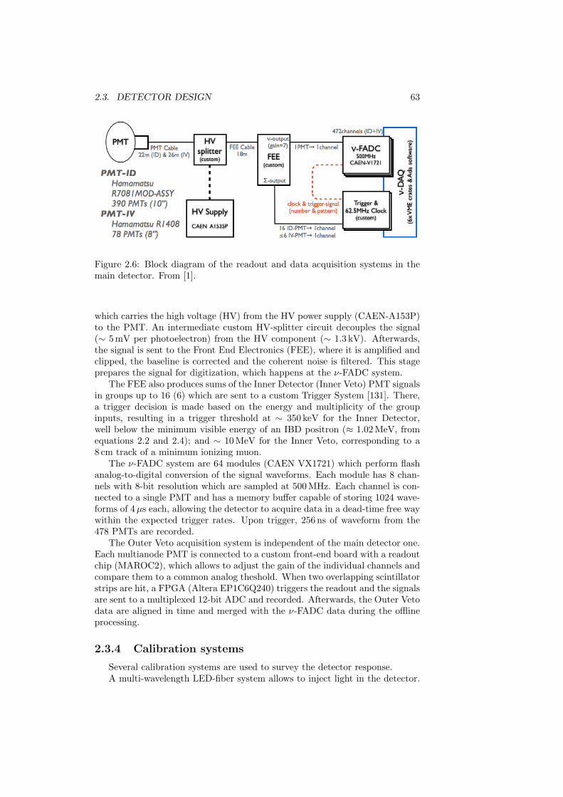
2.3. DETECTOR DESIGN 63
Figure 2.6: Block diagram of the readout and data acquisition systems in themain detector. From [1].
which carries the high voltage (HV) from the HV power supply (CAEN-A153P)to the PMT. An intermediate custom HV-splitter circuit decouples the signal(∼ 5 mV per photoelectron) from the HV component (∼ 1.3 kV). Afterwards,the signal is sent to the Front End Electronics (FEE), where it is amplified andclipped, the baseline is corrected and the coherent noise is filtered. This stageprepares the signal for digitization, which happens at the ν-FADC system.
The FEE also produces sums of the Inner Detector (Inner Veto) PMT signalsin groups up to 16 (6) which are sent to a custom Trigger System [131]. There,a trigger decision is made based on the energy and multiplicity of the groupinputs, resulting in a trigger threshold at ∼ 350 keV for the Inner Detector,well below the minimum visible energy of an IBD positron (≈ 1.02 MeV, fromequations 2.2 and 2.4); and ∼ 10 MeV for the Inner Veto, corresponding to a8 cm track of a minimum ionizing muon.
The ν-FADC system are 64 modules (CAEN VX1721) which perform flashanalog-to-digital conversion of the signal waveforms. Each module has 8 chan-nels with 8-bit resolution which are sampled at 500 MHz. Each channel is con-nected to a single PMT and has a memory buffer capable of storing 1024 wave-forms of 4µs each, allowing the detector to acquire data in a dead-time free waywithin the expected trigger rates. Upon trigger, 256 ns of waveform from the478 PMTs are recorded.
The Outer Veto acquisition system is independent of the main detector one.Each multianode PMT is connected to a custom front-end board with a readoutchip (MAROC2), which allows to adjust the gain of the individual channels andcompare them to a common analog theshold. When two overlapping scintillatorstrips are hit, a FPGA (Altera EP1C6Q240) triggers the readout and the signalsare sent to a multiplexed 12-bit ADC and recorded. Afterwards, the Outer Vetodata are aligned in time and merged with the ν-FADC data during the offlineprocessing.
2.3.4 Calibration systems
Several calibration systems are used to survey the detector response.A multi-wavelength LED-fiber system allows to inject light in the detector.
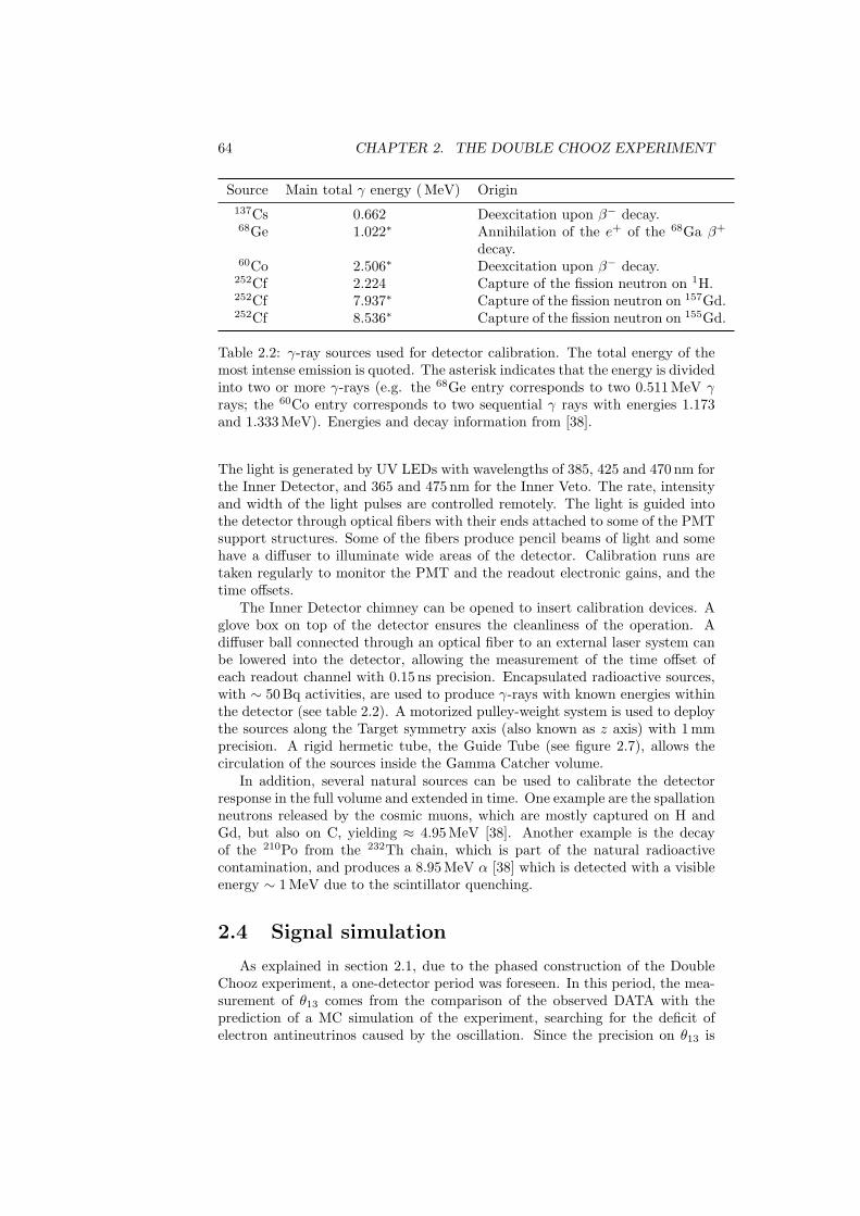
64 CHAPTER 2. THE DOUBLE CHOOZ EXPERIMENT
Source Main total γ energy ( MeV) Origin137Cs 0.662 Deexcitation upon β− decay.68Ge 1.022∗ Annihilation of the e+ of the 68Ga β+
decay.60Co 2.506∗ Deexcitation upon β− decay.
252Cf 2.224 Capture of the fission neutron on 1H.252Cf 7.937∗ Capture of the fission neutron on 157Gd.252Cf 8.536∗ Capture of the fission neutron on 155Gd.
Table 2.2: γ-ray sources used for detector calibration. The total energy of themost intense emission is quoted. The asterisk indicates that the energy is dividedinto two or more γ-rays (e.g. the 68Ge entry corresponds to two 0.511 MeV γrays; the 60Co entry corresponds to two sequential γ rays with energies 1.173and 1.333 MeV). Energies and decay information from [38].
The light is generated by UV LEDs with wavelengths of 385, 425 and 470 nm forthe Inner Detector, and 365 and 475 nm for the Inner Veto. The rate, intensityand width of the light pulses are controlled remotely. The light is guided intothe detector through optical fibers with their ends attached to some of the PMTsupport structures. Some of the fibers produce pencil beams of light and somehave a diffuser to illuminate wide areas of the detector. Calibration runs aretaken regularly to monitor the PMT and the readout electronic gains, and thetime offsets.
The Inner Detector chimney can be opened to insert calibration devices. Aglove box on top of the detector ensures the cleanliness of the operation. Adiffuser ball connected through an optical fiber to an external laser system canbe lowered into the detector, allowing the measurement of the time offset ofeach readout channel with 0.15 ns precision. Encapsulated radioactive sources,with ∼ 50 Bq activities, are used to produce γ-rays with known energies withinthe detector (see table 2.2). A motorized pulley-weight system is used to deploythe sources along the Target symmetry axis (also known as z axis) with 1 mmprecision. A rigid hermetic tube, the Guide Tube (see figure 2.7), allows thecirculation of the sources inside the Gamma Catcher volume.
In addition, several natural sources can be used to calibrate the detectorresponse in the full volume and extended in time. One example are the spallationneutrons released by the cosmic muons, which are mostly captured on H andGd, but also on C, yielding ≈ 4.95 MeV [38]. Another example is the decayof the 210Po from the 232Th chain, which is part of the natural radioactivecontamination, and produces a 8.95 MeV α [38] which is detected with a visibleenergy ∼ 1 MeV due to the scintillator quenching.
2.4 Signal simulation
As explained in section 2.1, due to the phased construction of the DoubleChooz experiment, a one-detector period was foreseen. In this period, the mea-surement of θ13 comes from the comparison of the observed DATA with theprediction of a MC simulation of the experiment, searching for the deficit ofelectron antineutrinos caused by the oscillation. Since the precision on θ13 is
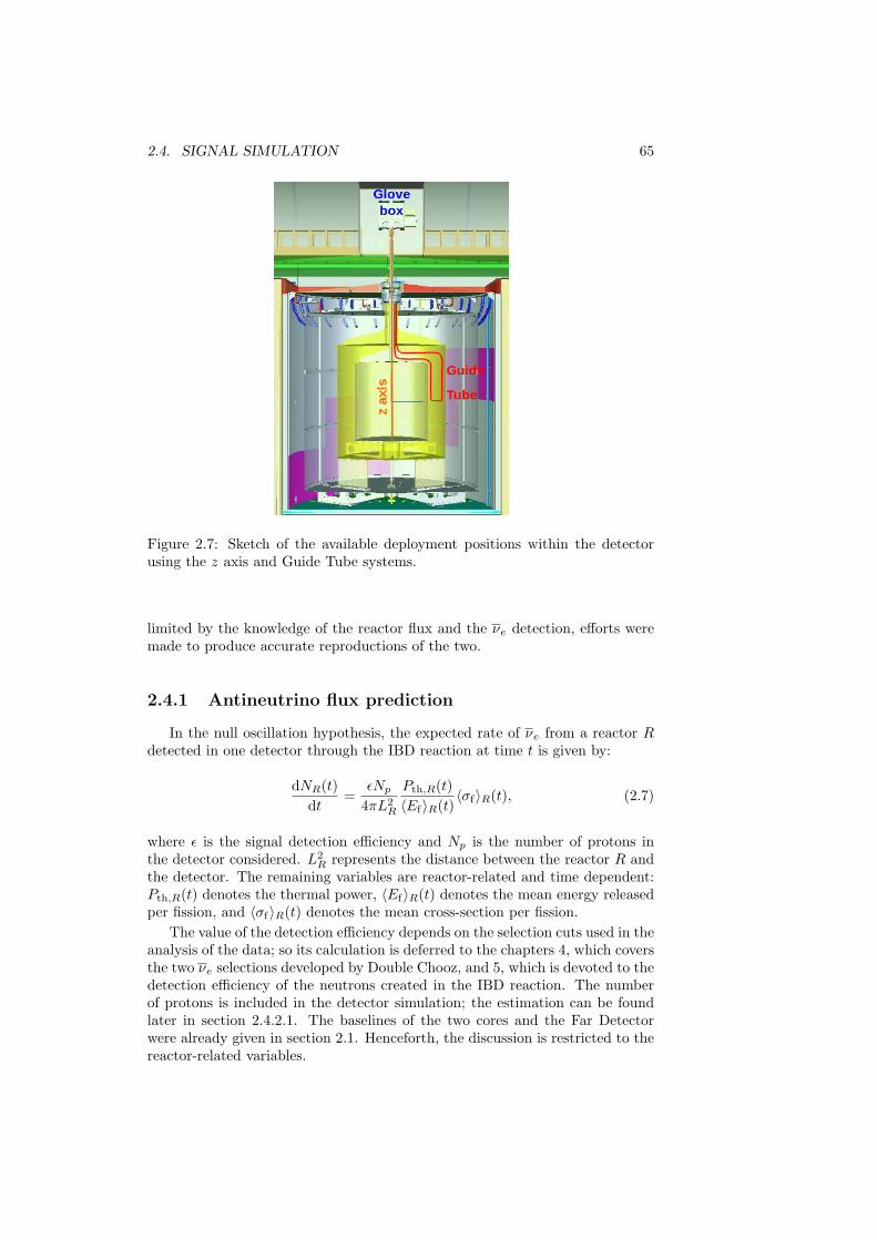
2.4. SIGNAL SIMULATION 65
Figure 2.7: Sketch of the available deployment positions within the detectorusing the z axis and Guide Tube systems.
limited by the knowledge of the reactor flux and the νe detection, efforts weremade to produce accurate reproductions of the two.
2.4.1 Antineutrino flux prediction
In the null oscillation hypothesis, the expected rate of νe from a reactor Rdetected in one detector through the IBD reaction at time t is given by:
dNR(t)dt
=εNp
4πL2R
Pth,R(t)〈Ef〉R(t)
〈σf〉R(t), (2.7)
where ε is the signal detection efficiency and Np is the number of protons inthe detector considered. L2
R represents the distance between the reactor R andthe detector. The remaining variables are reactor-related and time dependent:Pth,R(t) denotes the thermal power, 〈Ef〉R(t) denotes the mean energy releasedper fission, and 〈σf〉R(t) denotes the mean cross-section per fission.
The value of the detection efficiency depends on the selection cuts used in theanalysis of the data; so its calculation is deferred to the chapters 4, which coversthe two νe selections developed by Double Chooz, and 5, which is devoted to thedetection efficiency of the neutrons created in the IBD reaction. The numberof protons is included in the detector simulation; the estimation can be foundlater in section 2.4.2.1. The baselines of the two cores and the Far Detectorwere already given in section 2.1. Henceforth, the discussion is restricted to thereactor-related variables.
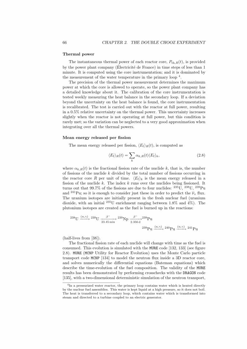
66 CHAPTER 2. THE DOUBLE CHOOZ EXPERIMENT
Thermal power
The instantaneous thermal power of each reactor core, Pth,R(t), is providedby the power plant company (Electricite de France) in time steps of less than 1minute. It is computed using the core instrumentation; and it is dominated bythe measurement of the water temperature in the primary loop 4.
The precision of the thermal power measurement determines the maximumpower at which the core is allowed to operate, so the power plant company hasa detailed knowledge about it. The calibration of the core instrumentation istested weekly measuring the heat balance in the secondary loop. If a deviationbeyond the uncertainty on the heat balance is found, the core instrumentationis recalibrated. The test is carried out with the reactor at full power, resultingin a 0.5% relative uncertainty on the thermal power. This uncertainty increasesslightly when the reactor is not operating at full power, but this condition israrely met; so the variation can be neglected to a very good approximation whenintegrating over all the thermal powers.
Mean energy released per fission
The mean energy released per fission, 〈Ef〉R(t), is computed as
〈Ef〉R(t) =∑k
αk,R(t)〈Ef〉k, (2.8)
where αk,R(t) is the fractional fission rate of the nuclide k, that is, the numberof fissions of the nuclide k divided by the total number of fissions occurring inthe reactor core R per unit of time. 〈Ef〉k is the mean energy released in afission of the nuclide k. The index k runs over the nuclides being fissioned. Itturns out that 99.7% of the fissions are due to four nuclides: 235U, 238U, 239Puand 241Pu; so it is enough to consider just these in order to predict the νe flux.The uranium isotopes are initially present in the fresh nuclear fuel (uraniumdioxide, with an initial 235U enrichment ranging between 1.8% and 4%). Theplutonium isotopes are created as the fuel is burned up in the reactions:
238U(n,γ)−−−→ 239U
β−−−−−−−→23.45 min
239Npβ−−−−−→
2.356 d
239Pu
239Pu(n,γ)−−−→ 240Pu
(n,γ)−−−→ 241Pu
(half-lives from [38]).The fractional fission rate of each nuclide will change with time as the fuel is
consumed. This evolution is simulated with the MURE code [132, 133] (see figure2.8). MURE (MCNP Utility for Reactor Evolution) uses the Monte Carlo particletransport code MCNP [134] to model the neutron flux inside a 3D reactor core,and solves numerically the differential equations (Bateman equations) whichdescribe the time-evolution of the fuel composition. The validity of the MUREresults has been demonstrated by performing crosschecks with the DRAGON code[135], with a two-dimensional deterministic simulation of the neutron transport,
4In a pressurized water reactor, the primary loop contains water which is heated directlyby the nuclear fuel assemblies. This water is kept liquid at a high pressure, so it does not boil.The heat is transferred to a secondary loop, which contains water which is transformed intosteam and directed to a turbine coupled to an electric generator.
2.4. SIGNAL SIMULATION 67
Nuclide 〈Ef〉k (MeV)235U 201.92± 0.46239Pu 209.99± 0.60238U 205.52± 0.96241Pu 213.60± 0.65
Table 2.3: Mean energy released per fission of nuclide. From [137].
and comparisons with the experimental data obtained from destructive assay offuel rods of the Takahama-3 reactor [136].
In order to model the reactor core accurately, the geometry and the materialswithin it must be defined in the MURE simulation. At the beginning of a reactorcycle, only one third of the fuel assemblies is fresh, the rest corresponds to fuelpartially used. The power plant company makes available the location and theinitial burnup of each assembly. By running the MURE and DRAGON simulationsfor the assemblies, it is possible to determine their initial composition; which isalso compared to the result of the power plant company simulation (APOLLO2-F).Then, MURE is used to simulate the time-evolution of the core in steps of 6–48hours, depending on the stability of the reactor operation.
The systematic uncertainties on the fractional fission rates are estimatedfrom the discrepancies found when the simulation inputs are varied. The sys-tematic uncertainty is dominated by the uncertainties on the neutron moderatordensity and the position of the control rods which are used to regulate the neu-tron flux inside the core. Other contributions are the thermal power, the boronconcentration in the primary loop (boron is a neutron absorber and is used tocontrol the fission rate), the neutron moderator temperature, the initial burnuperror, the nuclear databases and mean energy released per fission data consid-ered, and the statistical error of the Monte Carlo. Ultimately, the uncertaintyon the fractional fission rates implies a 0.8% uncertainty on the normalizationof the νe flux.
Returning to equation 2.8, the mean energy released per fission of a nuclideis found by computing the global Q value corresponding to the fission reactionand the subsequent β− decays of the fission products, which is known withgreat precision. To this global Q value, the energy deposited within the core bythe capture of fission neutrons not contributing to the chain reaction must beadded; and the energy taken away by the escaping νe and the undecayed fissionproducts must be subtracted [137]. The resulting values of the mean energiesreleased per fission of the four nuclides are given in table 2.3. The uncertaintyon them is translated into a 0.2% uncertainty on the νe rate.
Mean cross-section per fission
The mean cross-section per fission corresponds to the IBD reaction cross-section averaged over the full energy spectra of the νe emitted following a fission.It is written as
〈σf〉R(t) =∑k
αk,R(t)〈σf〉k, (2.9)
where αk,R(t) is the aforedescribed fractional fission rate of the nuclide k, and〈σf〉k is the mean cross-section per fission of the nuclide k, which is computed
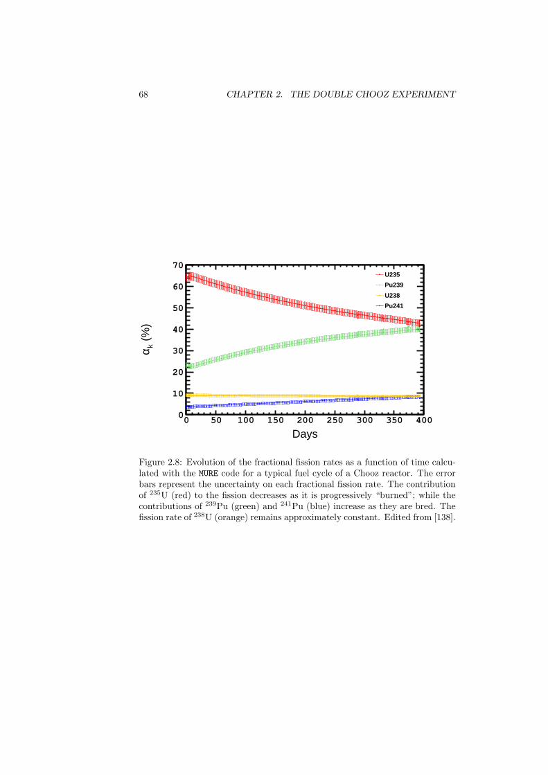
68 CHAPTER 2. THE DOUBLE CHOOZ EXPERIMENT
Days0 50 100 150 200 250 300 350 400
(%
)kα
0
10
20
30
40
50
60
70U235
Pu239
U238
Pu241
Figure 2.8: Evolution of the fractional fission rates as a function of time calcu-lated with the MURE code for a typical fuel cycle of a Chooz reactor. The errorbars represent the uncertainty on each fractional fission rate. The contributionof 235U (red) to the fission decreases as it is progressively “burned”; while thecontributions of 239Pu (green) and 241Pu (blue) increase as they are bred. Thefission rate of 238U (orange) remains approximately constant. Edited from [138].
2.4. SIGNAL SIMULATION 69
as
〈σf〉k =
∞∫0
Sk(Eνe)σIBD(Eνe)dEνe . (2.10)
σIBD(Eνe) is the IBD cross-section (equation 2.3) and Sk(Eνe) is the cumulatedenergy spectrum of all the νe emitted upon a fission of the nuclide k.
When a nuclide fissions stimulated by a neutron capture, it usually splits intotwo lighter nuclei, known as the fission products. These are unstable neutron-rich nuclei which undergo several β− decays, in which the νe are produced,before reaching stability (typically, each fission product decays thrice, resultingin 6 νe per fission).
Since there are not measurements of the fission product νe spectra withthe required precision, measurements of the electron spectra are used instead,which are then converted into νe spectra. For the fissile nuclides 235U, 239Puand 241Pu, the cumulated electron spectra from references [139, 140, 141] areused. These spectra are obtained by exposing thin films enriched with one ofthe fissile nuclides to the thermal neutron flux of the research reactor at theInstitut Laue-Langevin (ILL), and analyzing the electron spectrum with a mag-netic β spectrometer. The conversion to νe spectrum is carried out accordingto reference [98] by fitting virtual β branches—functions with the shape of anhypothetical allowed5 branch with an effective nuclear charge whose parameters(normalization, endpoint energy) are determined by the fit—to the electronspectrum, which are then converted into νe spectra invoking energy conserva-tion. A correction accounting for the off-equilibrium effects arising due to thelimited exposure of the films to the neutron flux at ILL (up to ∼ 2 days) incontrast to the much longer irradiation time inside a reactor like the ones atChooz (∼ 1 year) is also included [114].
The fissionable nuclide 238U has a negligible fission cross-section for thermalneutrons, which prevented a measurement at the ILL reactor. A recent mea-surement of the cumulated electron spectrum of 238U using a fast neutron beamat the Forschungsreaktor Munchen II (FRM II) neutron source is used [142].The low statistics of the electron spectrum at high energy preclude the use ofthe method based on virtual β branches, so the conversion into an νe spec-trum is made with a transfer function. This transfer function is computed usingthe measured cumulated electron spectrum of 235U [140] and a correspondingνe spectrum calculated by an ab initio approach—summation of the individ-ual νe spectra produced by the numerous branches of β− decays of the 235Ufission products, which are obtained from electron spectroscopy experimentaldata [114]. The 238U νe spectral data from reference [142] is restricted to the2.875 − 7.625 MeV energy range, so an extrapolation to lower and higher en-ergies is made by combination of an exponential-polynomial fit to the spectraldata and the ab initio spectrum for 238U [143], whose uncertainty is reducedby expressing it as a relative spectrum to other ab initio spectra (239Pu and241Pu), which is then made absolute using the spectra from [98].
As it can be concluded from the previous explanation, the obtention of theνe spectra is rather complicated, what makes the mean cross-section per fission
5The shape is further corrected by considering the finite size of the nucleus, the screeningof the nuclear charge due to the atomic electrons, radiative corrections and the effect of weakmagnetism.
70 CHAPTER 2. THE DOUBLE CHOOZ EXPERIMENT
the dominant source of systematic uncertainty on the νe flux. This uncertaintyvaries with the antineutrino energy, but it is at the level of 3% of the νe nor-malization. In order to improve the precision of the θ13 measurement duringthe one-detector phase of the experiment, the measurement of the mean cross-section per fission at the Bugey4 experiment [144], 〈σf〉B4 is used. In this case,the mean cross-section per fission (equation 2.9) is rewritten as
〈σf〉R(t) = 〈σf〉B4 +∑k
(αk,R(t)− αB4k )〈σf〉k, (2.11)
where αB4k is the published fractional fission rate of the nuclide k in the Bugey
reactor.Bugey4 was a short-baseline (15 m) reactor experiment which made a precise
measurement of the mean cross-section per fission, 〈σf〉B4 = (5.752 ± 0.081) ·10−43 cm2/fission (1.4% relative uncertainty). Because the composition of theBugey reactor was very similar to the ones of the Chooz reactors, the termbetween brackets of equation 2.11 is very small, thus suppressing the contri-bution of 〈σf〉k to the normalization uncertainty, which changes to 0.2%. Inaddition, an hypothetical deficit due to the oscillation of the νe into a fourthsterile antineutrino with a squared mass difference ∆m2
41 & 1 eV2 (as suggestedby the anomalies discussed in section 1.4) would be already included in theBugey4 measurement, rendering the θ13 oscillation fit unaffected by such sterileantineutrino. In a certain sense, the Bugey4 experiment serves as an effectivenear detector until the actual Double Chooz Near Detector is ready.
In the preceding discussion, only the expected rate resulting from integra-tion over the complete νe energy spectrum has been considered. However,the expected shape is also relevant since the oscillation probability is energy-dependent. In order to have a prediction of the detected νe flux binned in νeenergy, equation 2.7 must be modified to
dNi,R(t)dt
=εNp
4πL2R
Pth,R(t)〈Ef〉R(t)
×
×
(〈σf〉B4 +
∑k(αk,R(t)− αB4
k )〈σf〉k∑k αk,R(t)〈σf〉k
∑k
αk,R(t)〈σf〉i,k
),
(2.12)
where the index i represents the i-th bin, corresponding to the νe energy interval[Ei, Ei + ∆Ei). This requires to define the mean cross-section per fission of thenuclide k in the energy bin i as:
〈σf〉i,k =
Ei+∆Ei∫Ei
Sk(Eνe)σIBD(Eνe)dEνe . (2.13)
Double Chooz custom Monte Carlo event generator, DCRxtrTools [145], gen-erates νe according to equation 2.12 for each of the detector runs used in the os-cillation analysis, reading the time-dependent reactor variables (thermal powerand fractional fission rates) from a database. It also assigns an νe interactionvertex with a proton of the simulated detector, and produces the positron andthe neutron resulting from the IBD reaction with the proper kinematics [123].
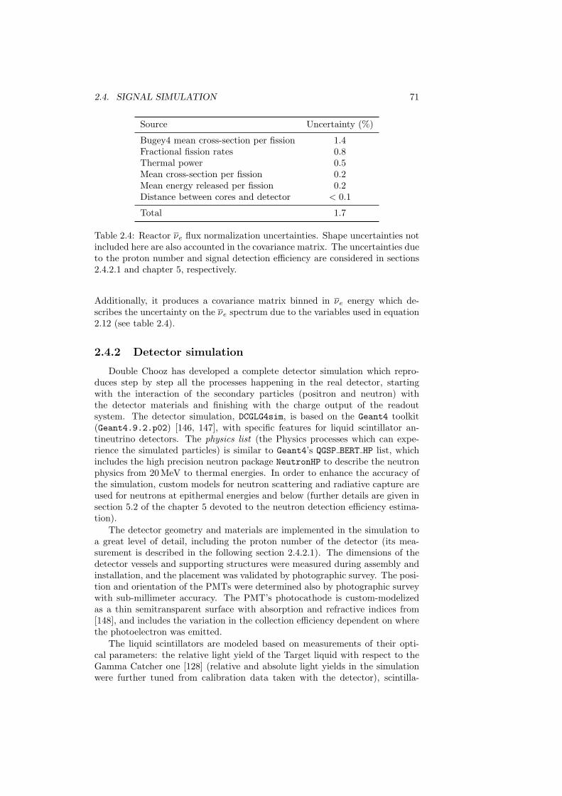
2.4. SIGNAL SIMULATION 71
Source Uncertainty (%)
Bugey4 mean cross-section per fission 1.4Fractional fission rates 0.8Thermal power 0.5Mean cross-section per fission 0.2Mean energy released per fission 0.2Distance between cores and detector < 0.1
Total 1.7
Table 2.4: Reactor νe flux normalization uncertainties. Shape uncertainties notincluded here are also accounted in the covariance matrix. The uncertainties dueto the proton number and signal detection efficiency are considered in sections2.4.2.1 and chapter 5, respectively.
Additionally, it produces a covariance matrix binned in νe energy which de-scribes the uncertainty on the νe spectrum due to the variables used in equation2.12 (see table 2.4).
2.4.2 Detector simulation
Double Chooz has developed a complete detector simulation which repro-duces step by step all the processes happening in the real detector, startingwith the interaction of the secondary particles (positron and neutron) withthe detector materials and finishing with the charge output of the readoutsystem. The detector simulation, DCGLG4sim, is based on the Geant4 toolkit(Geant4.9.2.p02) [146, 147], with specific features for liquid scintillator an-tineutrino detectors. The physics list (the Physics processes which can expe-rience the simulated particles) is similar to Geant4’s QGSP BERT HP list, whichincludes the high precision neutron package NeutronHP to describe the neutronphysics from 20 MeV to thermal energies. In order to enhance the accuracy ofthe simulation, custom models for neutron scattering and radiative capture areused for neutrons at epithermal energies and below (further details are given insection 5.2 of the chapter 5 devoted to the neutron detection efficiency estima-tion).
The detector geometry and materials are implemented in the simulation toa great level of detail, including the proton number of the detector (its mea-surement is described in the following section 2.4.2.1). The dimensions of thedetector vessels and supporting structures were measured during assembly andinstallation, and the placement was validated by photographic survey. The posi-tion and orientation of the PMTs were determined also by photographic surveywith sub-millimeter accuracy. The PMT’s photocathode is custom-modelizedas a thin semitransparent surface with absorption and refractive indices from[148], and includes the variation in the collection efficiency dependent on wherethe photoelectron was emitted.
The liquid scintillators are modeled based on measurements of their opti-cal parameters: the relative light yield of the Target liquid with respect to theGamma Catcher one [128] (relative and absolute light yields in the simulationwere further tuned from calibration data taken with the detector), scintilla-
72 CHAPTER 2. THE DOUBLE CHOOZ EXPERIMENT
tor emission spectrum, photon emission time probabilities, attenuation and re-emission probabilities [127], the ionization quenching (also known as Birk’s lawquenching) for electrons [149] and α particles [150] of different energies. Theoptical model also includes the measured refraction indices and reflectivities ofthe detector materials.
The readout system simulation, RoSS, reproduces the response of the fullchain (PMT, front-end electronics, flash-ADC, trigger and the data acquisitionsystems) to a photoelectron. Given the time when the PMT was hit by a photon,RoSS generates the corresponding digitized waveform. The model is based on anempirical probability density function which is built from measurements of theresponse of the components. The readout characteristics (gain, baseline, noise,single photoelectron width. . . ) are implemented channel-wise, so the output ofthe simulation exhibits a similar dispersion as the DATA.
2.4.2.1 Proton number
The number of free protons (the nuclei of hydrogen-1 atoms) determines thenumber of IBD interactions occurring in the detector. During the one-detectorphase, it is essential to know it accurately to have a reliable prediction of thenumber of νe expected (in the two-detector phase, the uncertainty in this valueis irrelevant since both detectors are identical).
The proton number in the Target liquid governs almost completely the num-ber of IBD interactions which end up with the neutron captured on Gd 6. Fromthe precise knowledge of the chemical composition and weight of the ingredientsused to produce the scintillator, the hydrogen fraction in the Target is calcu-lated to be 13.60 ± 0.04% by weight [127]. After measuring the total mass ofthe Target scintillator, (6.747± 0.020) · 1029 protons are estimated [69].
The proton number in the Gamma Catcher liquid is estimated differentlysince the hydrogen content of the mineral oil used is not precisely known. A CHN(Carbon, Hydrogen, Nitrogen) analysis found a hydrogen fraction of 14.6±0.2%by weight. The total volume of the Gamma Catcher scintillator is estimatedfrom geometrical measurements and converted into mass using the well-knowndensity, resulting in (1.582± 0.016) · 1030 protons [72].
Although the acrylic vessels and supporting structures do not scintillate,turning the positron kinetic energy invisible, the IBD interactions within themcan be detected when the γ-rays escape. The proton number for those bodiesis computed from their mass, assuming a 8.05% a hydrogen fraction (from themonomer formula C5H8O2). The results are (2.08± 0.48) · 1028 protons in theTarget and (6.96 ± 0.21) · 1028 protons in the Gamma Catcher acrylics [151];where the uncertainties have been estimated from the differences found with therespective numbers in the detector simulation.
The proton number in the Buffer is not relevant since it does not scintillate,so the IBD interactions within it are practically undetectable. Only the few νeinteracting close to the Gamma Catcher border have a chance to be detected(estimated in section 5.5.3). Since it is a skin effect, the hydrogen fraction ratherthan the total number of protons applies. A CHN analysis of the Buffer liquidfound a hydrogen fraction of 14.80±0.15% by weight. Hence, the proton number
6Except for a small number of neutrons created in the Gamma Catcher which migrate intothe Target, estimated in section 5.4.3
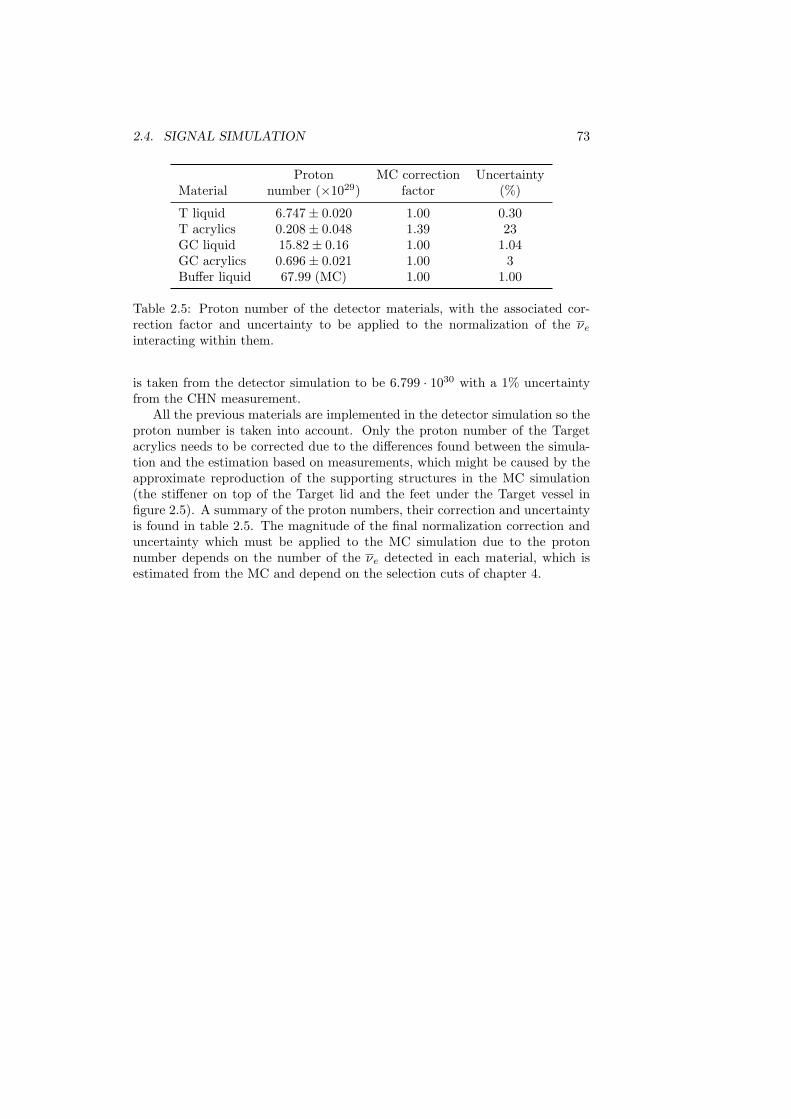
2.4. SIGNAL SIMULATION 73
Proton MC correction UncertaintyMaterial number (×1029) factor (%)
T liquid 6.747± 0.020 1.00 0.30T acrylics 0.208± 0.048 1.39 23GC liquid 15.82± 0.16 1.00 1.04GC acrylics 0.696± 0.021 1.00 3Buffer liquid 67.99 (MC) 1.00 1.00
Table 2.5: Proton number of the detector materials, with the associated cor-rection factor and uncertainty to be applied to the normalization of the νeinteracting within them.
is taken from the detector simulation to be 6.799 · 1030 with a 1% uncertaintyfrom the CHN measurement.
All the previous materials are implemented in the detector simulation so theproton number is taken into account. Only the proton number of the Targetacrylics needs to be corrected due to the differences found between the simula-tion and the estimation based on measurements, which might be caused by theapproximate reproduction of the supporting structures in the MC simulation(the stiffener on top of the Target lid and the feet under the Target vessel infigure 2.5). A summary of the proton numbers, their correction and uncertaintyis found in table 2.5. The magnitude of the final normalization correction anduncertainty which must be applied to the MC simulation due to the protonnumber depends on the number of the νe detected in each material, which isestimated from the MC and depend on the selection cuts of chapter 4.

74 CHAPTER 2. THE DOUBLE CHOOZ EXPERIMENT
Chapter 3
Event reconstruction
This chapter introduces the basic variables which are computed from thereconstruction of the event and which are later used in the selection of the IBDinteractions, explained in the next chapter.
A special emphasis is made on the energy. The oscillation probability isenergy-dependent (e.g. equation 1.54), so the antineutrino oscillations willleave a characteristic imprint on the electron antineutrino spectrum (and onthe closely related positron visible energy spectrum as equation 2.4 indicates)which should be used in order to exploit all the available empirical information tomeasure θ13 with the highest precision. This technique is known as Rate+Shapeanalysis, since both normalization and spectral shape are considered (this is dis-cussed further in section 6.2). In fact, Double Chooz was the first experimentto measure a non-null θ13 using a Rate+Shape analysis [69]. Moreover, becausethe background sources have energy spectra different from the νe one, their ratesin the selected IBD candidate sample (which contains both νe and backgroundevents) can be constrained from the total IBD candidates spectrum, increasingfurther the precision on θ13. In addition, the νe selection relies on energy cutsto select the positron and neutron signals from the IBD reaction, so the energyaccuracy has an explicit impact on the νe normalization. All these capabilitiesrequire to dominate the energy response of the detector.
The ambitious Monte Carlo simulation of the Double Chooz detector (in-troduced in section 2.4.2) produces signal waveforms equivalent to those of thereal detector; so the energy reconstruction is done in parallel for both DATAand MC. The visible energy per trigger, Evis, is obtained as
Evis = Nmpe · fmu (ρ, z) · fmMeV · fms (Emvis,, t) · fmqnl(E
mvis,), (3.1)
where the superscript m refers to DATA or MC. The first step is to obtainNm
pe, the total number of photoelectrons of the event, which is calculated fromthe reconstructed charge in each channel as explained in section 3.1 and thenconverted into photoelectrons as described in section 3.2.
The second step is the uniformity calibration, where fmu (ρ, z) is a functionof the reconstructed vertex coordinates ρ =
√x2 + y2 and z (introduced in
section 3.3) and corrects for the spatial dependence of the photoelectron yieldas described in section 3.4.
The third step is the conversion to energy units, carried out by fmMeV, aconversion factor from photoelectrons to MeV (introduced in section 3.5).
75
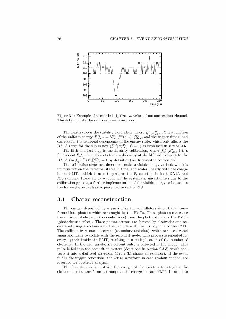
76 CHAPTER 3. EVENT RECONSTRUCTION
Time (ns)0 50 100 150 200 250
AD
C c
ount
s
205
206
207
208
209
210
211
212
Figure 3.1: Example of a recorded digitized waveform from one readout channel.The dots indicate the samples taken every 2 ns.
The fourth step is the stability calibration, where fms (Emvis,, t) is a functionof the uniform energy, Emvis, = Nm
pe ·fmu (ρ, z) ·fmMeV, and the trigger time t, andcorrects for the temporal dependence of the energy scale, which only affects theDATA (ergo for the simulation fMC
s (EMCvis,, t) = 1) as explained in section 3.6.
The fifth and last step is the linearity calibration, where fmqnl(Emvis,) is a
function of Emvis, and corrects the non-linearity of the MC with respect to theDATA (so fDATA
qnl (EDATAvis, ) = 1 by definition) as discussed in section 3.7.
The calibration steps just described render a visible energy variable which isuniform within the detector, stable in time, and scales linearly with the chargein the PMTs; which is used to perform the νe selection in both DATA andMC samples. However, to account for the systematic uncertainties due to thecalibration process, a further implementation of the visible energy to be used inthe Rate+Shape analysis is presented in section 3.8.
3.1 Charge reconstruction
The energy deposited by a particle in the scintillators is partially trans-formed into photons which are caught by the PMTs. These photons can causethe emission of electrons (photoelectrons) from the photocathode of the PMTs(photoelectric effect). These photoelectrons are focused by electrodes and ac-celerated using a voltage until they collide with the first dynode of the PMT.The collision frees more electrons (secondary emission), which are acceleratedagain and made to collide with the second dynode. This process is repeated forevery dynode inside the PMT, resulting in a multiplication of the number ofelectrons. In the end, an electric current pulse is collected in the anode. Thispulse is fed into the acquisition system (described in section 2.3.3) which con-verts it into a digitized waveform (figure 3.1 shows an example). If the eventfulfills the trigger conditions, the 256 ns waveform in each readout channel arerecorded for posterior analysis.
The first step to reconstruct the energy of the event is to integrate theelectric current waveforms to compute the charge in each PMT. In order to
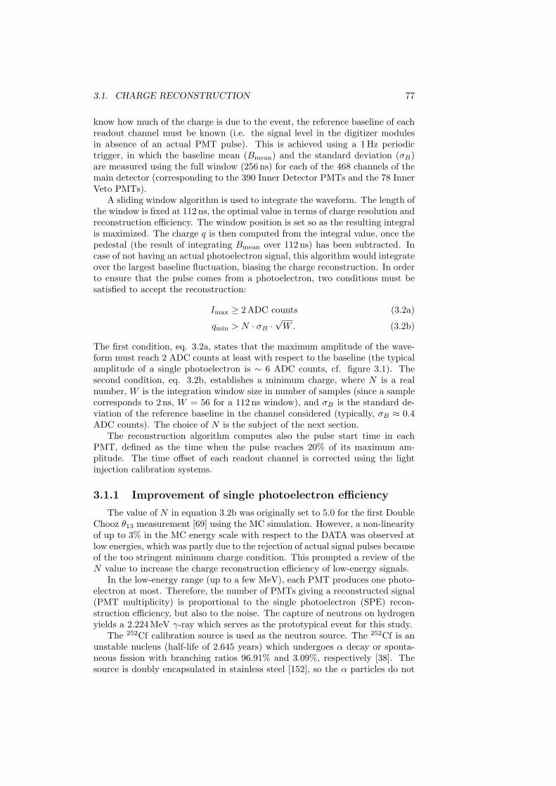
3.1. CHARGE RECONSTRUCTION 77
know how much of the charge is due to the event, the reference baseline of eachreadout channel must be known (i.e. the signal level in the digitizer modulesin absence of an actual PMT pulse). This is achieved using a 1 Hz periodictrigger, in which the baseline mean (Bmean) and the standard deviation (σB)are measured using the full window (256 ns) for each of the 468 channels of themain detector (corresponding to the 390 Inner Detector PMTs and the 78 InnerVeto PMTs).
A sliding window algorithm is used to integrate the waveform. The length ofthe window is fixed at 112 ns, the optimal value in terms of charge resolution andreconstruction efficiency. The window position is set so as the resulting integralis maximized. The charge q is then computed from the integral value, once thepedestal (the result of integrating Bmean over 112 ns) has been subtracted. Incase of not having an actual photoelectron signal, this algorithm would integrateover the largest baseline fluctuation, biasing the charge reconstruction. In orderto ensure that the pulse comes from a photoelectron, two conditions must besatisfied to accept the reconstruction:
Imax ≥ 2 ADC counts (3.2a)
qmin > N · σB ·√W. (3.2b)
The first condition, eq. 3.2a, states that the maximum amplitude of the wave-form must reach 2 ADC counts at least with respect to the baseline (the typicalamplitude of a single photoelectron is ∼ 6 ADC counts, cf. figure 3.1). Thesecond condition, eq. 3.2b, establishes a minimum charge, where N is a realnumber, W is the integration window size in number of samples (since a samplecorresponds to 2 ns, W = 56 for a 112 ns window), and σB is the standard de-viation of the reference baseline in the channel considered (typically, σB ≈ 0.4ADC counts). The choice of N is the subject of the next section.
The reconstruction algorithm computes also the pulse start time in eachPMT, defined as the time when the pulse reaches 20% of its maximum am-plitude. The time offset of each readout channel is corrected using the lightinjection calibration systems.
3.1.1 Improvement of single photoelectron efficiency
The value of N in equation 3.2b was originally set to 5.0 for the first DoubleChooz θ13 measurement [69] using the MC simulation. However, a non-linearityof up to 3% in the MC energy scale with respect to the DATA was observed atlow energies, which was partly due to the rejection of actual signal pulses becauseof the too stringent minimum charge condition. This prompted a review of theN value to increase the charge reconstruction efficiency of low-energy signals.
In the low-energy range (up to a few MeV), each PMT produces one photo-electron at most. Therefore, the number of PMTs giving a reconstructed signal(PMT multiplicity) is proportional to the single photoelectron (SPE) recon-struction efficiency, but also to the noise. The capture of neutrons on hydrogenyields a 2.224 MeV γ-ray which serves as the prototypical event for this study.
The 252Cf calibration source is used as the neutron source. The 252Cf is anunstable nucleus (half-life of 2.645 years) which undergoes α decay or sponta-neous fission with branching ratios 96.91% and 3.09%, respectively [38]. Thesource is doubly encapsulated in stainless steel [152], so the α particles do not
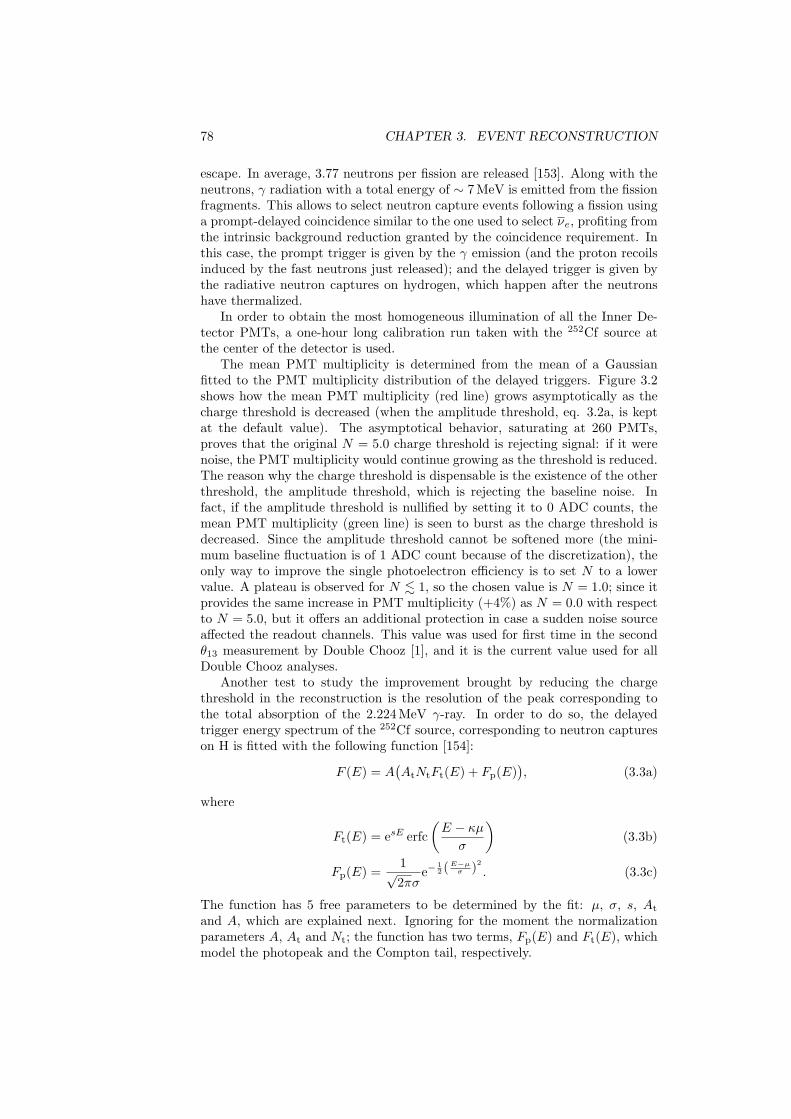
78 CHAPTER 3. EVENT RECONSTRUCTION
escape. In average, 3.77 neutrons per fission are released [153]. Along with theneutrons, γ radiation with a total energy of ∼ 7 MeV is emitted from the fissionfragments. This allows to select neutron capture events following a fission usinga prompt-delayed coincidence similar to the one used to select νe, profiting fromthe intrinsic background reduction granted by the coincidence requirement. Inthis case, the prompt trigger is given by the γ emission (and the proton recoilsinduced by the fast neutrons just released); and the delayed trigger is given bythe radiative neutron captures on hydrogen, which happen after the neutronshave thermalized.
In order to obtain the most homogeneous illumination of all the Inner De-tector PMTs, a one-hour long calibration run taken with the 252Cf source atthe center of the detector is used.
The mean PMT multiplicity is determined from the mean of a Gaussianfitted to the PMT multiplicity distribution of the delayed triggers. Figure 3.2shows how the mean PMT multiplicity (red line) grows asymptotically as thecharge threshold is decreased (when the amplitude threshold, eq. 3.2a, is keptat the default value). The asymptotical behavior, saturating at 260 PMTs,proves that the original N = 5.0 charge threshold is rejecting signal: if it werenoise, the PMT multiplicity would continue growing as the threshold is reduced.The reason why the charge threshold is dispensable is the existence of the otherthreshold, the amplitude threshold, which is rejecting the baseline noise. Infact, if the amplitude threshold is nullified by setting it to 0 ADC counts, themean PMT multiplicity (green line) is seen to burst as the charge threshold isdecreased. Since the amplitude threshold cannot be softened more (the mini-mum baseline fluctuation is of 1 ADC count because of the discretization), theonly way to improve the single photoelectron efficiency is to set N to a lowervalue. A plateau is observed for N . 1, so the chosen value is N = 1.0; since itprovides the same increase in PMT multiplicity (+4%) as N = 0.0 with respectto N = 5.0, but it offers an additional protection in case a sudden noise sourceaffected the readout channels. This value was used for first time in the secondθ13 measurement by Double Chooz [1], and it is the current value used for allDouble Chooz analyses.
Another test to study the improvement brought by reducing the chargethreshold in the reconstruction is the resolution of the peak corresponding tothe total absorption of the 2.224 MeV γ-ray. In order to do so, the delayedtrigger energy spectrum of the 252Cf source, corresponding to neutron captureson H is fitted with the following function [154]:
F (E) = A(AtNtFt(E) + Fp(E)
), (3.3a)
where
Ft(E) = esE erfc(E − κµσ
)(3.3b)
Fp(E) =1√2πσ
e−12 (E−µσ )2
. (3.3c)
The function has 5 free parameters to be determined by the fit: µ, σ, s, At
and A, which are explained next. Ignoring for the moment the normalizationparameters A, At and Nt; the function has two terms, Fp(E) and Ft(E), whichmodel the photopeak and the Compton tail, respectively.
3.1. CHARGE RECONSTRUCTION 79
N0 1 2 3 4 5 6 7 8
PM
T M
ultip
licity
240
260
280
300
320
340 2 ADC counts≥ maxI
0 ADC counts≥ maxI
Figure 3.2: Mean PMT multiplicity as a function of the parameter N of thereconstruction charge threshold (eq. 3.2b). Data from neutron captures onH using the 252Cf source. Red: maximum amplitude threshold (eq. 3.2a) atdefault value (2 ADC counts). Green: maximum amplitude threshold removed.
The function Fp(E) is a normalized Gaussian function with mean µ, whichcorresponds to the resulting energy of the photopeak after summing the re-constructed charges of the readout channels; and standard deviation σ, whichaccounts for the widening caused by the statistical and electronic noise. Theamplitude of the photopeak is controlled by the normalization parameter A.
The function Ft(E) is the outcome of convoluting an exponential function todescribe the shape of the Compton tail with a Gaussian function to model thenoise, which is parametrized using the same σ as in the photopeak. This resultsin the exponential being multiplied by the complementary error function,
erfc(x) = 1− erf(x) =2√π
∞∫x
e−t2dt. (3.4)
The Compton tail is modeled by esE , where s controls the steepness of thetail. The position of the Compton edge, (κ · µ), is left as a function of thephotopeak energy, µ. Using the expression for the maximum energy transfer inthe Compton scattering, the value of κ can be calculated as
κ = 1− 11 + µ
me(1− cosπ)
, (3.5)
where me is the electron mass. The photopeak of the neutron capture on H hasµ = 2.224 MeV, so κ = 0.897. The amplitude of the Compton tail is expressedas a fraction of the photopeak amplitude, A, using the fractional tail amplitudeAt. In order to do so, Ft(E) is normalized to unity in the interval (0, µ + 2σ)
80 CHAPTER 3. EVENT RECONSTRUCTION
/ ndf 2χ 22.8 / 13Prob 0.04409A 6.5± 398.4
µ 0.002± 2.224 σ 0.0017± 0.1321 tA 0.0088± 0.1049
s 0.2612± 0.9165
Energy (MeV*t)0 1 2 3 4 5 6
Ent
ries/
100
KeV
10
210
310 / ndf 2χ 22.8 / 13
Prob 0.04409A 6.5± 398.4
µ 0.002± 2.224 σ 0.0017± 0.1321 tA 0.0088± 0.1049
s 0.2612± 0.9165
Figure 3.3: Fit of the function in eq. 3.3 to the energy spectrum of the 252Cfneutrons captured on H (the parameter N of the reconstruction charge thresholdis set to 5.0).
using the normalization constant Nt, which is defined as
Nt ≡
µ+2σ∫0
Ft(x)dx
−1
= s
(esx erfc
(x− κµσ
)− eκµs+σ
2s2/4 erf(κµ− x+ σ2s/2
σ
))∣∣∣∣∣µ+2σ
0
.
The resolution is estimated as the ratio between the width (σfit) and themean (Efit) energy of the H capture peak, which are taken from the best-fitvalues of the parameters σ and µ of the function in equation 3.3 (see figure 3.3for an example of a fit).
Figure 3.4 shows the resolution of the peak as a function of the parameterN of the charge threshold. It is observed how the resolution worsens when thecharge threshold is increased, as a result of considering a smaller number ofchannels for the calorimetric sum. On the contrary, the resolution improvesslightly when the charge threshold is diminished (for N = 1.0, the improvementwith respect to N = 5.0 is (2.3± 1.8)%). If reducing the charge threshold hadled to the reconstruction of noise, the resolution would have deteriorated. Thisresult confirms the conclusion of the PMT multiplicity study.
3.2 Photoelectron conversion
The total number of photoelectrons produced by one event in the detector,Npe, is obtained from the sum of the number of photoelectrons of each channel,pei, where the subindex i denotes the i-th channel. The number of photoelec-trons in the i-th channel is calculated from the reconstructed charge qi, using a
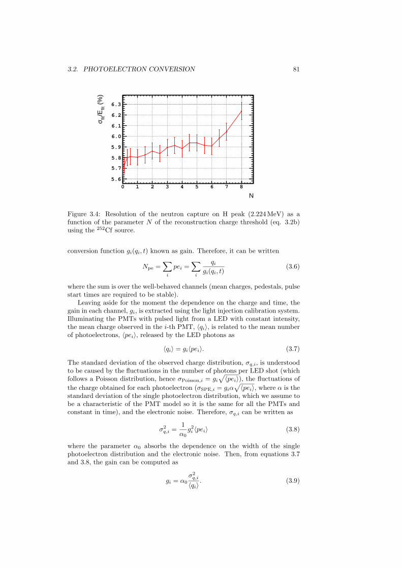
3.2. PHOTOELECTRON CONVERSION 81
N
0 1 2 3 4 5 6 7 8
(%
)fit
/Efitσ
5.6
5.7
5.8
5.9
6.0
6.1
6.2
6.3
Figure 3.4: Resolution of the neutron capture on H peak (2.224 MeV) as afunction of the parameter N of the reconstruction charge threshold (eq. 3.2b)using the 252Cf source.
conversion function gi(qi, t) known as gain. Therefore, it can be written
Npe =∑i
pei =∑i
qigi(qi, t)
(3.6)
where the sum is over the well-behaved channels (mean charges, pedestals, pulsestart times are required to be stable).
Leaving aside for the moment the dependence on the charge and time, thegain in each channel, gi, is extracted using the light injection calibration system.Illuminating the PMTs with pulsed light from a LED with constant intensity,the mean charge observed in the i-th PMT, 〈qi〉, is related to the mean numberof photoelectrons, 〈pei〉, released by the LED photons as
〈qi〉 = gi〈pei〉. (3.7)
The standard deviation of the observed charge distribution, σq,i, is understoodto be caused by the fluctuations in the number of photons per LED shot (whichfollows a Poisson distribution, hence σPoisson,i = gi
√〈pei〉), the fluctuations of
the charge obtained for each photoelectron (σSPE,i = giα√〈pei〉, where α is the
standard deviation of the single photoelectron distribution, which we assume tobe a characteristic of the PMT model so it is the same for all the PMTs andconstant in time), and the electronic noise. Therefore, σq,i can be written as
σ2q,i =
1α0g2i 〈pei〉 (3.8)
where the parameter α0 absorbs the dependence on the width of the singlephotoelectron distribution and the electronic noise. Then, from equations 3.7and 3.8, the gain can be computed as
gi = α0
σ2q,i
〈qi〉. (3.9)
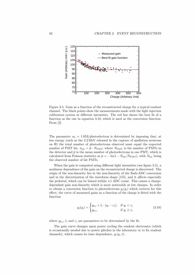
82 CHAPTER 3. EVENT RECONSTRUCTION
Charge (Arbitrary Unit)0 100 200 300 400 500 600
Gai
n (A
rbitr
ary
Uni
t / p
.e.)
70
75
80
85
90
95
100
105
110
115
120
Measured gainBest-fit gain function
Figure 3.5: Gain as a function of the reconstructed charge for a typical readoutchannel. The black points show the measurements made with the light injectioncalibration system at different intensities. The red line shows the best fit of afunction as the one in equation 3.10, which is used as the conversion function.From [2].
The parameter α0 = 1.053/photoelectron is determined by imposing that, atlow energy (such as the 2.2 MeV released in the capture of spallation neutronson H) the total number of photoelectrons observed must equal the expectednumber of PMT hit, πhit = µ ·NPMT; where NPMT is the number of PMTs inthe detector and µ is the mean number of photoelectrons in one PMT, which iscalculated from Poisson statistics as µ = − ln(1−Nhit/NPMT), with Nhit beingthe observed number of hit PMTs.
When the gain is computed using different light intensities (see figure 3.5), anonlinear dependence of the gain on the reconstructed charge is discovered. Theorigin of the non-linearity lies in the non-linearity of the flash-ADC conversionand in the discretization of the waveform shape [155], and it affects especiallythe pedestal, which can be biased within ±1 ADC count. This causes a charge-dependent gain non-linearity which is more noticeable at low charges. In orderto obtain a conversion function to photoelectrons gi(qi) which corrects for thiseffect, the curve of measured gains as a function of the charge is fitted with thefunction
gi(qi) =
g0,i + li · (qi − ci), if qi < ci
g0,i, if qi ≥ ci(3.10)
where g0,i, li and ci are parameters to be determined by the fit.
The gain curve changes upon power cycling the readout electronics (whichis occasionally needed due to power glitches in the laboratory or to fix readoutchannels), which causes its time dependence, gi(qi, t).
3.3. VERTEX RECONSTRUCTION 83
3.3 Vertex reconstruction
The reconstruction of the event vertex (either the positron energy depositionor the radiative capture of the neutron) in the Inner Detector is used in theνe selection (reviewed in next chapter) to correlate the prompt and delayedtriggers, but it is also used to correct the event energy for the variations due toits position within the detector as explained in next section.
The Double Chooz vertex reconstruction algorithm is called RecoBAMA. Fora point-like event defined by the set X = (x0, y0, z0, t0,Φ), where (x0, y0, z0) arethe spatial coordinates within the detector, t0 is the event time and Φ is the lightintensity per solid angle (expressed in photons/steradian); the RecoBAMA vertexreconstruction is given by the X which maximizes the following likelihood:
L(X) =∏i
(pei=0)
fpe(0;µi)∏i
(pei>0)
fpe(pei;µi)ft(ti; τi, µi), (3.11)
where fpe(pei;µi) is the probability to measure the observed number of photo-electrons pei in the i-th PMT when the expected number is µi; and ft(ti; τi, µi)is the probability to measure the event at time ti (corrected for the channeloffset) when the expected time is τi for the expected µi photoelectrons. Theexpected number of photoelectrons and time in the i-th PMT are predicted as
µi = Φ εi ΩiAi (3.12a)
τi = t0 +ricn
(3.12b)
where εi is the PMT quantum efficiency, Ωi is the solid angle subtended by thePMT for a vertex located at a distance ri, Ai is the light transmission amplitude(which includes the effects of the light attenuation as it traverses detector andof the dependence on the angle of incidence, tuned using the radioactive sourcedata); and cn is the effective speed of light in the Inner Detector. The likelihoodtakes into account the possibility that some PMTs do not receive a photonby dividing the product into the PMTs which have not been hit (pei = 0)and therefore do not have time information, and those which have been hit(pei > 0). The probability functions fpe and ft, and the effective speed of lightcn are derived from the calibration data taken with the laser source.
In practice, instead of finding the X which maximizes equation 3.11, thenegative log-likelihood function
FV (X) = − lnL(X) (3.13)
is minimized, which is equivalent. The value of FV at the minimum is a measureof the goodness of the reconstruction and can be used to discriminate signal frombackground (explained in section 4.1.3.1).
3.4 Uniformity calibration
The Inner Detector response is not completely homogeneous due to geomet-rical effects (e.g. PMT positions and coverage) and the different media inside,so the total number of photoelectrons depends on the position of the event
84 CHAPTER 3. EVENT RECONSTRUCTION
within the detector. In order to correct for this spatial dependence, a unifor-mity calibration map is applied, fu(ρ, z), which is a function of the reconstructedcoordinates ρ =
√x2 + y2 and z. The map is defined such that the corrected
photoelectron number, Npe(ρ, z) · fu(ρ, z), equals the one at the center of thedetector, Npe(ρ = 0, z = 0), for the same physics event:
fu(ρ, z) =Npe(ρ = 0, z = 0)
Npe(ρ, z)
∣∣∣∣∣n−H
, (3.14)
where the subscript n−H indicates that the map is built using the peak of thephotoelectron spectrum produced by the 2.2 MeV γ-ray released in the captureof a neutron on a hydrogen nucleus. The DATA map is made using the spallationneutrons produced after the passage of a muon through the detector, and the MCmap is made using simulated IBD neutrons (see figure 3.6). Both are abundantsources of neutrons which fully explore the scintillator volumes (Target andGamma Catcher).
The data used to evaluate the systematic uncertainty on the visible energybecause of a residual non-uniformity are different in the two νe selections (oneusing the IBD neutrons captured on Gd, another using the IBD neutrons cap-tured on H).
In the case of the Gd selection, the remaining non-uniformity in the Targetbetween DATA and MC is taken as the systematic uncertainty. It is found tobe 0.36%, estimated as the standard deviation of the relative differences acrossthe Target volume between the DATA and MC maps built using the ∼ 8 MeVenergy released in the capture of a neutron on a gadolinium nucleus, after thevisible energy calibration (equation 3.1) is completed.
In the case of the H selection, the systematic uncertainty cannot be assessedusing gadolinium-based maps, since these do not represent the Gamma Catchervolume. Therefore, a different strategy is followed resorting to hydrogen-capturemaps. However, the uniformity calibration maps are already made using neu-trons captured on H. For the MC this is not a problem, since an statisticallyindependent MC can be generated. For the DATA, an auxiliary uniformitycalibration map is made just for the uncertainty estimation using half of thespallation neutron sample (selected to be evenly distributed in time). This aux-iliary map is verified to agree with the official one which uses the full sample. Asin the previous case, the systematic uncertainty is estimated from the residualnon-uniformity after the full visible energy calibration is completed; but thistime evaluated in the whole detector (Target and Gamma Catcher) using theother half of the spallation neutron sample as DATA (which have been correctedusing the auxiliary map) and the independent MC sample. The standard devi-ation of the relative differences between the two results in a 0.25% uncertainty.
3.5 Energy conversion
The photoelectron-to-megaelectronvolt conversion factor, fMeV, is deter-mined from the position of the photopeak in the energy spectrum of neutroncaptures on hydrogen, resulting from the deployment of the 252Cf source atthe center of the detector (see figure 3.7). The energy spectrum is fitted with
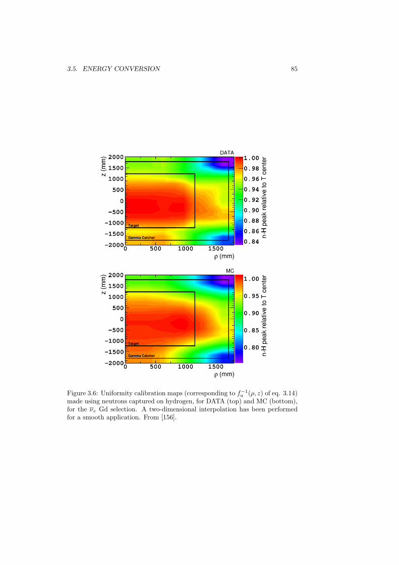
3.5. ENERGY CONVERSION 85
Figure 3.6: Uniformity calibration maps (corresponding to f−1u (ρ, z) of eq. 3.14)
made using neutrons captured on hydrogen, for DATA (top) and MC (bottom),for the νe Gd selection. A two-dimensional interpolation has been performedfor a smooth application. From [156].
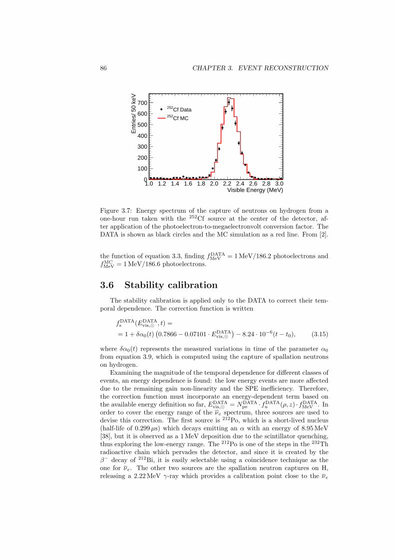
86 CHAPTER 3. EVENT RECONSTRUCTION
Visible Energy (MeV)1.0 1.2 1.4 1.6 1.8 2.0 2.2 2.4 2.6 2.8 3.0
Ent
ries/
50
keV
0
100
200
300
400
500
600
700Cf Data252
Cf MC252
Figure 3.7: Energy spectrum of the capture of neutrons on hydrogen from aone-hour run taken with the 252Cf source at the center of the detector, af-ter application of the photoelectron-to-megaelectronvolt conversion factor. TheDATA is shown as black circles and the MC simulation as a red line. From [2].
the function of equation 3.3, finding fDATAMeV = 1 MeV/186.2 photoelectrons and
fMCMeV = 1 MeV/186.6 photoelectrons.
3.6 Stability calibration
The stability calibration is applied only to the DATA to correct their tem-poral dependence. The correction function is written
fDATAs (EDATA
vis, , t) =
= 1 + δα0(t)(0.7866− 0.07101 · EDATA
vis,)− 8.24 · 10−6(t− t0), (3.15)
where δα0(t) represents the measured variations in time of the parameter α0
from equation 3.9, which is computed using the capture of spallation neutronson hydrogen.
Examining the magnitude of the temporal dependence for different classes ofevents, an energy dependence is found: the low energy events are more affecteddue to the remaining gain non-linearity and the SPE inefficiency. Therefore,the correction function must incorporate an energy-dependent term based onthe available energy definition so far, EDATA
vis, = NDATApe ·fDATA
u (ρ, z) ·fDATAMeV . In
order to cover the energy range of the νe spectrum, three sources are used todevise this correction. The first source is 212Po, which is a short-lived nucleus(half-life of 0.299µs) which decays emitting an α with an energy of 8.95 MeV[38], but it is observed as a 1 MeV deposition due to the scintillator quenching,thus exploring the low-energy range. The 212Po is one of the steps in the 232Thradioactive chain which pervades the detector, and since it is created by theβ− decay of 212Bi, it is easily selectable using a coincidence technique as theone for νe. The other two sources are the spallation neutron captures on H,releasing a 2.22 MeV γ-ray which provides a calibration point close to the νe
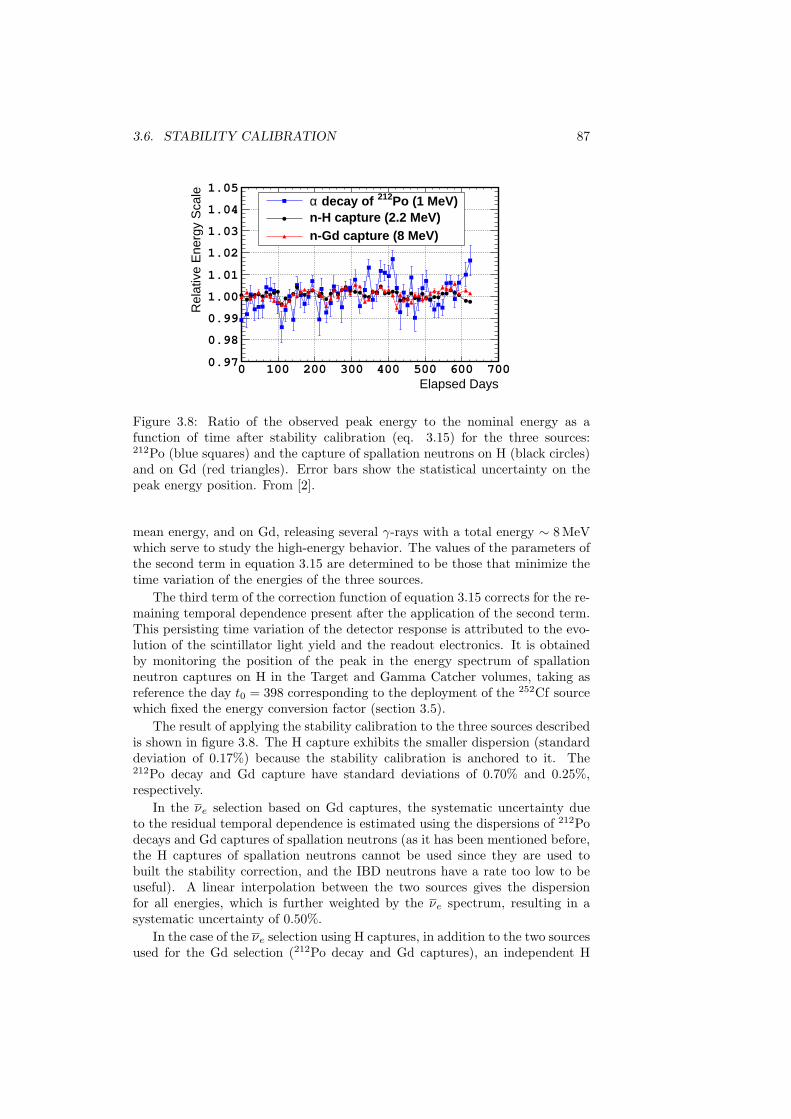
3.6. STABILITY CALIBRATION 87
Elapsed Days0 100 200 300 400 500 600 700
Rel
ativ
e E
nerg
y S
cale
0.97
0.98
0.99
1.00
1.01
1.02
1.03
1.04
1.05Po (1 MeV)212 decay of α
n-H capture (2.2 MeV)n-Gd capture (8 MeV)
Figure 3.8: Ratio of the observed peak energy to the nominal energy as afunction of time after stability calibration (eq. 3.15) for the three sources:212Po (blue squares) and the capture of spallation neutrons on H (black circles)and on Gd (red triangles). Error bars show the statistical uncertainty on thepeak energy position. From [2].
mean energy, and on Gd, releasing several γ-rays with a total energy ∼ 8 MeVwhich serve to study the high-energy behavior. The values of the parameters ofthe second term in equation 3.15 are determined to be those that minimize thetime variation of the energies of the three sources.
The third term of the correction function of equation 3.15 corrects for the re-maining temporal dependence present after the application of the second term.This persisting time variation of the detector response is attributed to the evo-lution of the scintillator light yield and the readout electronics. It is obtainedby monitoring the position of the peak in the energy spectrum of spallationneutron captures on H in the Target and Gamma Catcher volumes, taking asreference the day t0 = 398 corresponding to the deployment of the 252Cf sourcewhich fixed the energy conversion factor (section 3.5).
The result of applying the stability calibration to the three sources describedis shown in figure 3.8. The H capture exhibits the smaller dispersion (standarddeviation of 0.17%) because the stability calibration is anchored to it. The212Po decay and Gd capture have standard deviations of 0.70% and 0.25%,respectively.
In the νe selection based on Gd captures, the systematic uncertainty dueto the residual temporal dependence is estimated using the dispersions of 212Podecays and Gd captures of spallation neutrons (as it has been mentioned before,the H captures of spallation neutrons cannot be used since they are used tobuilt the stability correction, and the IBD neutrons have a rate too low to beuseful). A linear interpolation between the two sources gives the dispersionfor all energies, which is further weighted by the νe spectrum, resulting in asystematic uncertainty of 0.50%.
In the case of the νe selection using H captures, in addition to the two sourcesused for the Gd selection (212Po decay and Gd captures), an independent H
88 CHAPTER 3. EVENT RECONSTRUCTION
capture source is obtained from the IBD neutrons, so that a linear interpolationcan be built using three points instead of two. Weighting by the νe spectrumas before, this results in a systematic uncertainty of 0.33%.
3.7 Linearity calibration
The linearity calibration is applied to the energy of the MC simulation tocorrect for its non-linearity displayed relative to the DATA. The origin of thisnon-linearity is twofold: part is related to the reconstruction of the event charge,so it is referred to as charge non-linearity; and part is related to the generationof light in the scintillator by the event and is called light non-linearity correc-tion. The charge non-linearity arises from biases in the modeling of the readoutsystem and the charge reconstruction algorithm used for the simulation, thusaffecting all Inner Detector triggers. The light non-linearity originates in themodeling of the scintillator light properties. Therefore, it depends on the parti-cle being considered and the detector volume where it interacted, since Targetand Gamma Catcher have different scintillator mixtures.
For the abovesaid reasons, the calibration of the two non-linearities is donedifferently: the charge non-linearity is corrected for all events using a functionfMC
qnl (EMCvis,), which is a function of the visible energy prior to this correction,
EMCvis, = NMC
pe · fMCu (ρ, z) · fMC
MeV. Regarding the light non-linearity, insteadof including a correction in the visible energy definition (equation 3.1), it iscorrected in the Rate+Shape analysis (section 3.8). The explanation of how thetwo corrections are obtained is given in the rest of this section.
Charge non-linearity
The charge-non-linearity correction function fMCqnl (EMC
vis,) is extracted ana-lyzing the DATA of the neutron captures, either on H or on Gd, obtained fromthe deployment of the 252Cf source at the center of the detector and the corre-sponding MC simulation. Even though the total energy released upon neutroncapture on H (one γ-ray of 2.22 MeV) and on Gd (typically three or four γ-rays totaling ∼ 8 MeV [157, 158]) are different, the average energy per γ-ray(∼ 2.2 MeV) is very similar. Therefore, the scintillator response for the twocases is almost the same and the DATA-MC discrepancy found between the twocan be attributed to a non-linearity in the total charge obtention. The followingfunction is used to correct for such discrepancy:
fMCqnl (EMC
vis,) = 0.0023 · EMCvis, + 0.9949. (3.16)
The systematic uncertainty on this correction, δfMCqnl (EMC
vis ), is estimatedfrom the DATA-MC residual non-linearity observed in the 252Cf data deployedalong the detector z axis, after the fMC
qnl (EMCvis,) correction has been applied. It
can be parametrized as a a linear function,
δfMCqnl (EMC
vis ) = bqnl + cqnl · EMCvis , (3.17)
with bqnl = (1.004 ± 0.004) and cqnl = (−0.0001 ± 0.0006) MeV−1, where theparameter uncertainties are given by their standard deviation found when all thez axis positions are used. The correlation between the bqnl and cqnl parameters
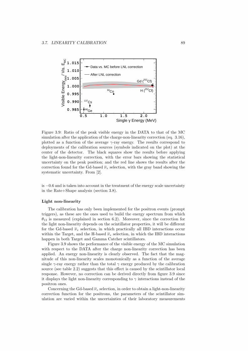
3.7. LINEARITY CALIBRATION 89
Energy (MeV)γSingle 0.5 1.0 1.5 2.0
MC
/ Vis
. Eda
taV
isib
le E
nerg
y
0.985
0.990
0.995
1.000
1.005
1.010
1.015Data vs. MC before LNL correction
After LNL correction
Cs137
Ge68
Cf)252H (Co60
Cf)252Gd (
Figure 3.9: Ratio of the peak visible energy in the DATA to that of the MCsimulation after the application of the charge-non-linearity correction (eq. 3.16),plotted as a function of the average γ-ray energy. The results correspond todeployments of the calibration sources (symbols indicated on the plot) at thecenter of the detector. The black squares show the results before applyingthe light-non-linearity correction, with the error bars showing the statisticaluncertainty on the peak position; and the red line shows the results after thecorrection found for the Gd-based νe selection, with the gray band showing thesystematic uncertainty. From [2].
is −0.6 and is taken into account in the treatment of the energy scale uncertaintyin the Rate+Shape analysis (section 3.8).
Light non-linearity
The calibration has only been implemented for the positron events (prompttriggers), as these are the ones used to build the energy spectrum from whichθ13 is measured (explained in section 6.2). Moreover, since the correction forthe light non-linearity depends on the scintillator properties, it will be differentfor the Gd-based νe selection, in which practically all IBD interactions occurwithin the Target, and the H-based νe selection, in which the IBD interactionshappen in both Target and Gamma Catcher scintillators.
Figure 3.9 shows the performance of the visible energy of the MC simulationwith respect to the DATA after the charge non-linearity correction has beenapplied. An energy non-linearity is clearly observed. The fact that the mag-nitude of this non-linearity scales monotonically as a function of the averagesingle γ-ray energy rather than the total γ energy produced by the calibrationsource (see table 2.2) suggests that this effect is caused by the scintillator localresponse. However, no correction can be derived directly from figure 3.9 sinceit displays the light non-linearity corresponding to γ interactions instead of thepositron ones.
Concerning the Gd-based νe selection, in order to obtain a light-non-linearitycorrection function for the positrons, the parameters of the scintillator sim-ulation are varied within the uncertainties of their laboratory measurements
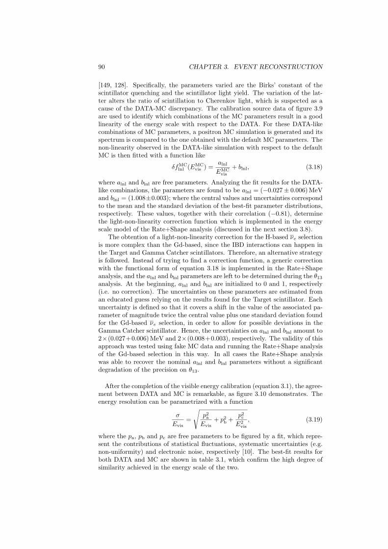
90 CHAPTER 3. EVENT RECONSTRUCTION
[149, 128]. Specifically, the parameters varied are the Birks’ constant of thescintillator quenching and the scintillator light yield. The variation of the lat-ter alters the ratio of scintillation to Cherenkov light, which is suspected as acause of the DATA-MC discrepancy. The calibration source data of figure 3.9are used to identify which combinations of the MC parameters result in a goodlinearity of the energy scale with respect to the DATA. For these DATA-likecombinations of MC parameters, a positron MC simulation is generated and itsspectrum is compared to the one obtained with the default MC parameters. Thenon-linearity observed in the DATA-like simulation with respect to the defaultMC is then fitted with a function like
δfMClnl (EMC
vis ) =alnl
EMCvis
+ blnl, (3.18)
where alnl and blnl are free parameters. Analyzing the fit results for the DATA-like combinations, the parameters are found to be alnl = (−0.027± 0.006) MeVand blnl = (1.008±0.003); where the central values and uncertainties correspondto the mean and the standard deviation of the best-fit parameter distributions,respectively. These values, together with their correlation (−0.81), determinethe light-non-linearity correction function which is implemented in the energyscale model of the Rate+Shape analysis (discussed in the next section 3.8).
The obtention of a light-non-linearity correction for the H-based νe selectionis more complex than the Gd-based, since the IBD interactions can happen inthe Target and Gamma Catcher scintillators. Therefore, an alternative strategyis followed. Instead of trying to find a correction function, a generic correctionwith the functional form of equation 3.18 is implemented in the Rate+Shapeanalysis, and the alnl and blnl parameters are left to be determined during the θ13
analysis. At the beginning, alnl and blnl are initialized to 0 and 1, respectively(i.e. no correction). The uncertainties on these parameters are estimated froman educated guess relying on the results found for the Target scintillator. Eachuncertainty is defined so that it covers a shift in the value of the associated pa-rameter of magnitude twice the central value plus one standard deviation foundfor the Gd-based νe selection, in order to allow for possible deviations in theGamma Catcher scintillator. Hence, the uncertainties on alnl and blnl amount to2×(0.027+0.006) MeV and 2×(0.008+0.003), respectively. The validity of thisapproach was tested using fake MC data and running the Rate+Shape analysisof the Gd-based selection in this way. In all cases the Rate+Shape analysiswas able to recover the nominal alnl and blnl parameters without a significantdegradation of the precision on θ13.
After the completion of the visible energy calibration (equation 3.1), the agree-ment between DATA and MC is remarkable, as figure 3.10 demonstrates. Theenergy resolution can be parametrized with a function
σ
Evis=
√p2
a
Evis+ p2
b +p2
c
E2vis
, (3.19)
where the pa, pb and pc are free parameters to be figured by a fit, which repre-sent the contributions of statistical fluctuations, systematic uncertainties (e.g.non-uniformity) and electronic noise, respectively [10]. The best-fit results forboth DATA and MC are shown in table 3.1, which confirm the high degree ofsimilarity achieved in the energy scale of the two.
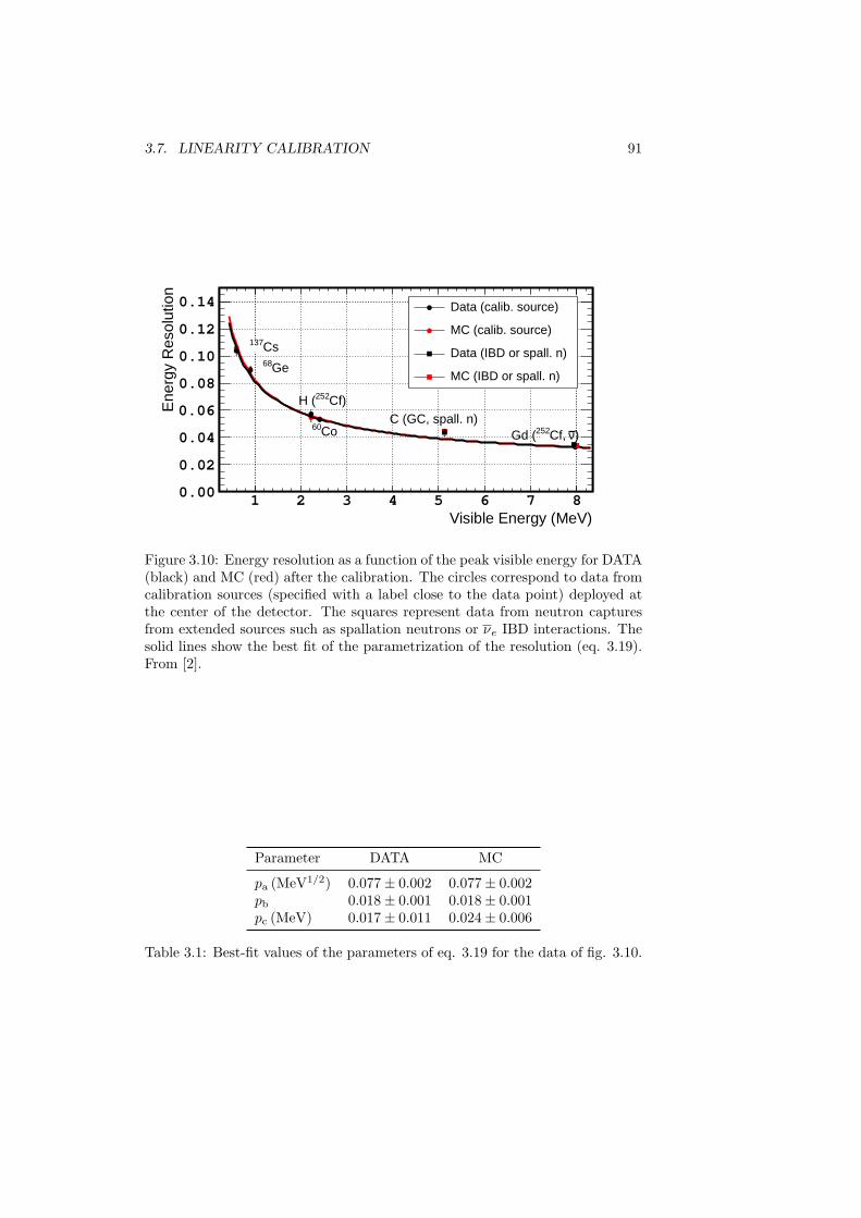
3.7. LINEARITY CALIBRATION 91
Visible Energy (MeV)1 2 3 4 5 6 7 8
Ene
rgy
Res
olut
ion
0.00
0.02
0.04
0.06
0.08
0.10
0.12
0.14
Cs137
Ge68
Cf)252H (
Co60)νCf, 252Gd (
C (GC, spall. n)
Data (calib. source)
MC (calib. source)
Data (IBD or spall. n)
MC (IBD or spall. n)
Figure 3.10: Energy resolution as a function of the peak visible energy for DATA(black) and MC (red) after the calibration. The circles correspond to data fromcalibration sources (specified with a label close to the data point) deployed atthe center of the detector. The squares represent data from neutron capturesfrom extended sources such as spallation neutrons or νe IBD interactions. Thesolid lines show the best fit of the parametrization of the resolution (eq. 3.19).From [2].
Parameter DATA MC
pa (MeV1/2) 0.077± 0.002 0.077± 0.002pb 0.018± 0.001 0.018± 0.001pc (MeV) 0.017± 0.011 0.024± 0.006
Table 3.1: Best-fit values of the parameters of eq. 3.19 for the data of fig. 3.10.
92 CHAPTER 3. EVENT RECONSTRUCTION
Parameter Gd selection H selection
bu 1.0000± 0.0036 1.0000± 0.0025bs 1.0000± 0.0050 1.0000± 0.0033bqnl 1.004± 0.004 1.004± 0.004cqnl (MeV−1) −0.0001± 0.0006 −0.0001± 0.0006alnl (MeV) −0.027± 0.006 0.000± 0.066blnl 1.008± 0.003 1.000± 0.021
Table 3.2: Summary of initialization values and uncertainties of the parametersof eq. 3.21 for the two νe selections.
3.8 Energy scale in the Rate+Shape analysis
Even after all the corrections described in this chapter are applied, a residualbias in the energy of the MC simulation might exist; which must be taken intoaccount when comparing the DATA and MC positron spectra to measure θ13
with the Rate+Shape analysis (section 6.2). This is achieved by treating thevisible energy of the MC simulation not as a fixed variable but as a floatingvariable which can be adjusted during the θ13 analysis, constrained by its un-certainty. In order to do so, the visible energy used in the oscillation analysis,EMC
vis,fit, is written as
EMCvis,fit = EMC
vis · δfMCu · δfMC
s · δfMCqnl (EMC
vis ) · δfMClnl (EMC
vis ) (3.20)
where EMCvis is the visible energy of equation 3.1. δfMC
u is the residual correctionto the MC energy due to the non-uniformity with respect to the DATA. Sincethe uniformity calibration (section 3.4) should have already corrected for thiseffect and no dependence on the visible energy is expected, δfMC
u can be writ-ten as δfMC
u = bu, with bu being a floating parameter which is initialized in thefit to 1.0 (no correction). The uncertainty on the bu parameter is the residualrelative non-uniformity between DATA and MC (see table 3.2). Analogously,δfMC
s is the residual correction to the MC energy due to the non-stability ofthe DATA in time. As before, the temporal dependence across all the energyrange is thought to be corrected by the stability calibration (section 3.6), soδfMC
s = bs, where bs is a floating parameter originally set to unity (no cor-rection), with an uncertainty given by the residual non-stability of the DATAenergy (see table 3.2). δfMC
qnl (EMCvis ) is the parametrization of the residual charge
non-linearity (equation 3.17) already presented in section 3.7. δfMClnl (EMC
vis ) isthe implementation of the light non-linearity correction (equation 3.18), whichhad been postponed until now.
Rewriting equation 3.20 explicitly in terms of the parameters
EMCvis,fit = EMC
vis · bu · bs ·(bqnl + cqnl · EMC
vis
)·(alnl
EMCvis
+ blnl
)(3.21)
and rearranging them, the visible energy in the fit can be modelized as aquadratic polynomial
EMCvis,fit = a′ + b′ · EMC
vis + c′ ·(EMC
vis
)2(3.22a)
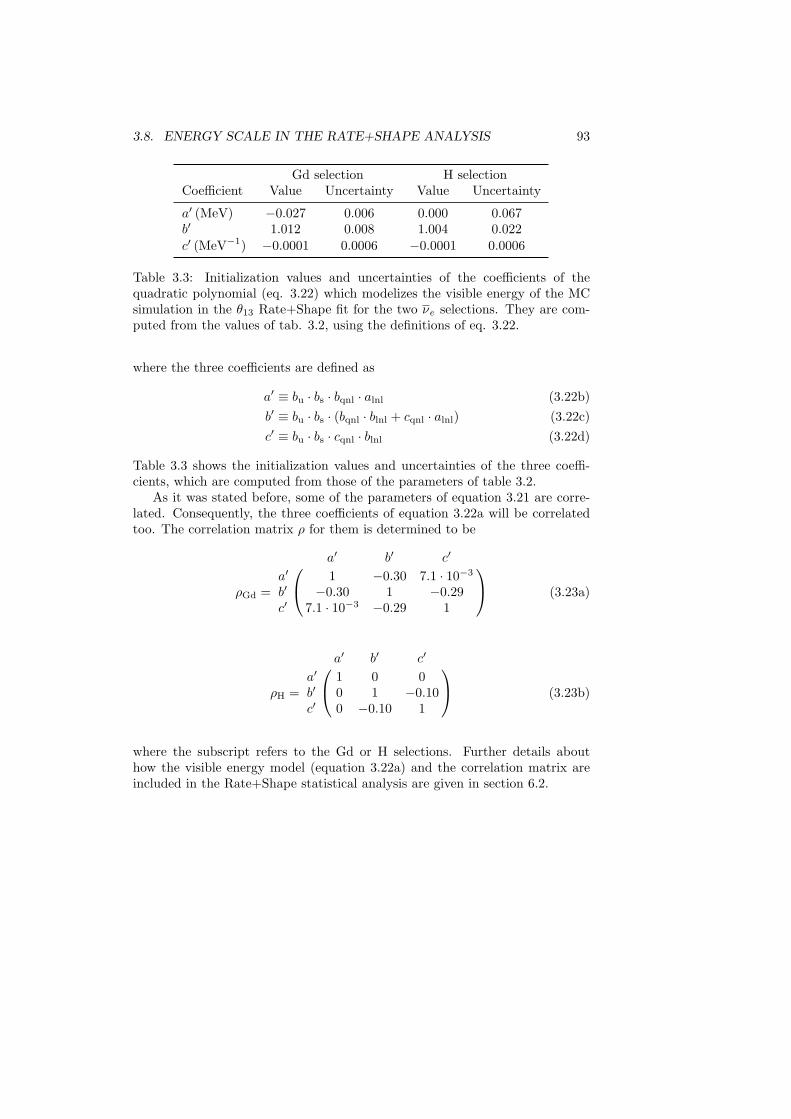
3.8. ENERGY SCALE IN THE RATE+SHAPE ANALYSIS 93
Gd selection H selectionCoefficient Value Uncertainty Value Uncertainty
a′ (MeV) −0.027 0.006 0.000 0.067b′ 1.012 0.008 1.004 0.022c′ (MeV−1) −0.0001 0.0006 −0.0001 0.0006
Table 3.3: Initialization values and uncertainties of the coefficients of thequadratic polynomial (eq. 3.22) which modelizes the visible energy of the MCsimulation in the θ13 Rate+Shape fit for the two νe selections. They are com-puted from the values of tab. 3.2, using the definitions of eq. 3.22.
where the three coefficients are defined as
a′ ≡ bu · bs · bqnl · alnl (3.22b)b′ ≡ bu · bs · (bqnl · blnl + cqnl · alnl) (3.22c)c′ ≡ bu · bs · cqnl · blnl (3.22d)
Table 3.3 shows the initialization values and uncertainties of the three coeffi-cients, which are computed from those of the parameters of table 3.2.
As it was stated before, some of the parameters of equation 3.21 are corre-lated. Consequently, the three coefficients of equation 3.22a will be correlatedtoo. The correlation matrix ρ for them is determined to be
ρGd =
a′ b′ c′
a′ 1 −0.30 7.1 · 10−3
b′ −0.30 1 −0.29c′ 7.1 · 10−3 −0.29 1
(3.23a)
ρH =
a′ b′ c′
a′ 1 0 0b′ 0 1 −0.10c′ 0 −0.10 1
(3.23b)
where the subscript refers to the Gd or H selections. Further details abouthow the visible energy model (equation 3.22a) and the correlation matrix areincluded in the Rate+Shape statistical analysis are given in section 6.2.

94 CHAPTER 3. EVENT RECONSTRUCTION
Chapter 4
Antineutrino selections
The Double Chooz collaboration has developed two selections of the electronantineutrinos which interact in the detector via inverse β-decay, νe + p→ e+ +n, depending on which nucleus captures the neutron produced, gadolinium orhydrogen (other nuclei have negligible neutron capture rates). The selectionspresented here were published in [2, 159], and they correspond to an endeavorto optimize previous selections using Gd captures [1] and H captures [72]. Thetwo selections have been kept as similar as possible in order to facilitate thecombination of the results on θ13.
The dichotomy posed by the neutron capture nucleus is reflected in the chap-ter layout: it is divided into two long sections, the first covering the Gd selection(section 4.1) and the second devoted to the H selection (section 4.2). Withineach selection, a similar structure is followed: firstly, the data analyzed are in-troduced. Secondly, the trigger preselection before searching for νe is described(sections 4.1.1 and 4.2.1). Thirdly, the cuts targeted to find the trigger coin-cidence which is characteristic of the IBD process are explained (sections 4.1.2and 4.2.2). Finally, the backgrounds hiding in the IBD selection are describedtogether with the specific vetoes developed against them, and the estimationof the remaining contamination (sections 4.1.3 and 4.2.3). Figure 4.1 shows ascheme with both antineutrino selections to be used as a guide for the chapter.
4.1 Gadolinium selection
The detector design is optimized for the IBD neutrons to be captured onGd. The Gd is only present in the scintillator of the innermost volume, theTarget, and it is surrounded by an unloaded scintillator, the Gamma Catcher,to improve the calorimetric response. In addition, the extremely high thermalneutron capture cross section of Gd offers a high signal detection efficiency.Finally, the energy released upon a radiative neutron capture on Gd is wellabove the typical energies of the natural radioactivity background, giving thisselection the highest signal to background ratio.
The Far Detector data used for the analysis amounts to 12305 runs takenbetween April 13th 2011 and January 15th 2013, totaling 489.51 days of run-time. After subtraction of the dead-time introduced by the muon and OV vetoes(described in sections 4.1.1.1 and 4.1.3.1, respectively), a live-time of 467.90 days
95
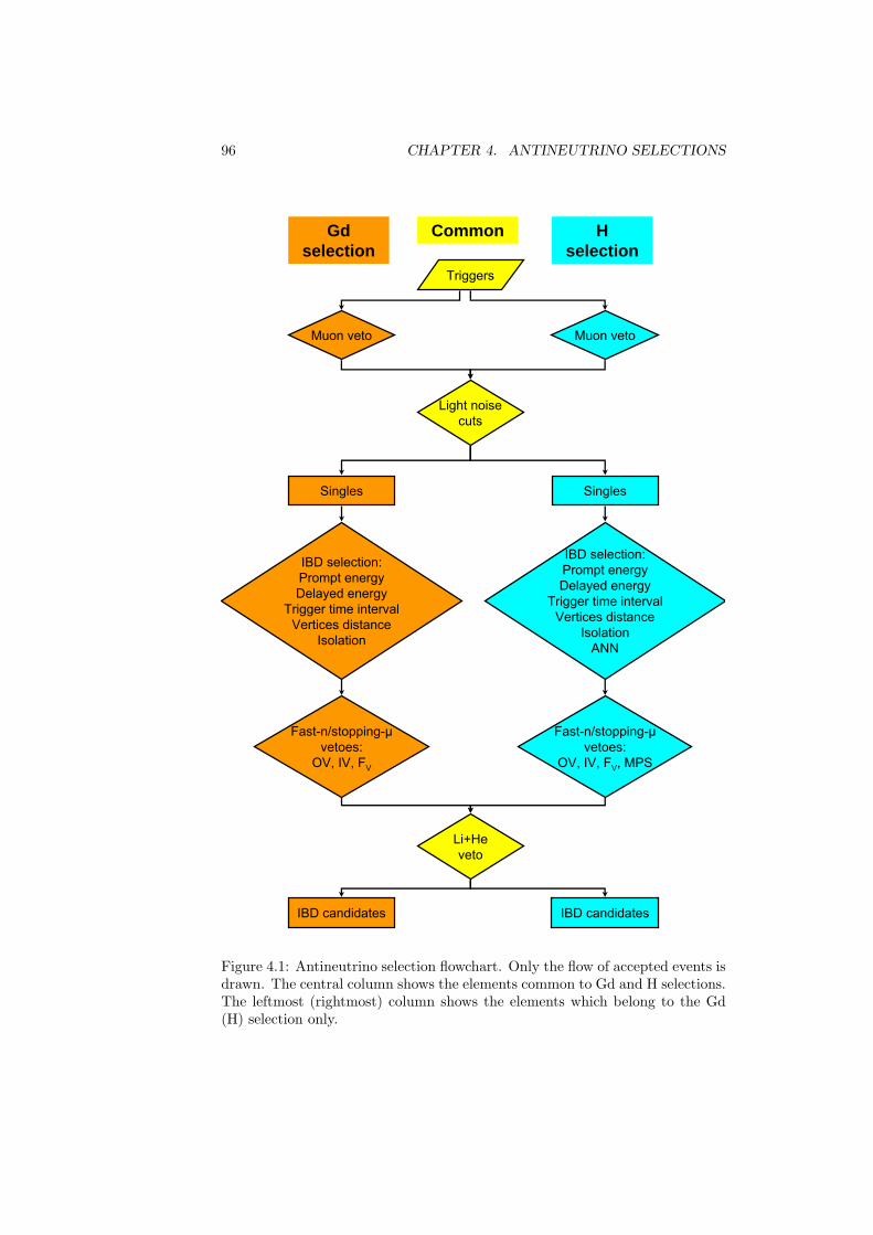
96 CHAPTER 4. ANTINEUTRINO SELECTIONS
Triggers
Muon
veto Muon
veto
Light noisecuts
IBD selection:Prompt energyDelayed energy
Trigger time intervalVertices distance
Isolation
Fast-n/stopping-μvetoes:
OV, IV, FV
Li+Heveto
IBD selection:Prompt energyDelayed energy
Trigger time intervalVertices distance
IsolationANN
Singles Singles
IBD candidates IBD candidates
Fast-n/stopping-μvetoes:
OV, IV, FV
, MPS
Gd selection
Common H selection
Figure 4.1: Antineutrino selection flowchart. Only the flow of accepted events isdrawn. The central column shows the elements common to Gd and H selections.The leftmost (rightmost) column shows the elements which belong to the Gd(H) selection only.
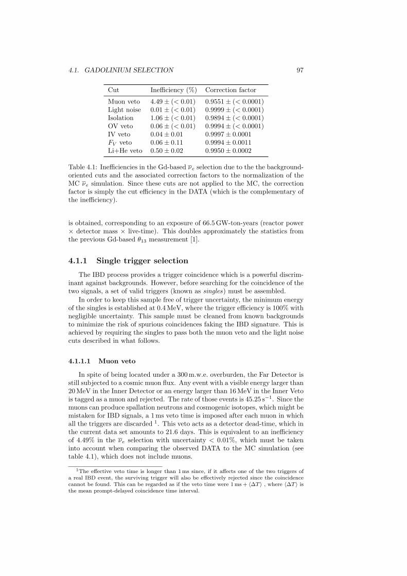
4.1. GADOLINIUM SELECTION 97
Cut Inefficiency (%) Correction factor
Muon veto 4.49± (< 0.01) 0.9551± (< 0.0001)Light noise 0.01± (< 0.01) 0.9999± (< 0.0001)Isolation 1.06± (< 0.01) 0.9894± (< 0.0001)OV veto 0.06± (< 0.01) 0.9994± (< 0.0001)IV veto 0.04± 0.01 0.9997± 0.0001FV veto 0.06± 0.11 0.9994± 0.0011Li+He veto 0.50± 0.02 0.9950± 0.0002
Table 4.1: Inefficiencies in the Gd-based νe selection due to the the background-oriented cuts and the associated correction factors to the normalization of theMC νe simulation. Since these cuts are not applied to the MC, the correctionfactor is simply the cut efficiency in the DATA (which is the complementary ofthe inefficiency).
is obtained, corresponding to an exposure of 66.5 GW-ton-years (reactor power× detector mass × live-time). This doubles approximately the statistics fromthe previous Gd-based θ13 measurement [1].
4.1.1 Single trigger selection
The IBD process provides a trigger coincidence which is a powerful discrim-inant against backgrounds. However, before searching for the coincidence of thetwo signals, a set of valid triggers (known as singles) must be assembled.
In order to keep this sample free of trigger uncertainty, the minimum energyof the singles is established at 0.4 MeV, where the trigger efficiency is 100% withnegligible uncertainty. This sample must be cleaned from known backgroundsto minimize the risk of spurious coincidences faking the IBD signature. This isachieved by requiring the singles to pass both the muon veto and the light noisecuts described in what follows.
4.1.1.1 Muon veto
In spite of being located under a 300 m.w.e. overburden, the Far Detector isstill subjected to a cosmic muon flux. Any event with a visible energy larger than20 MeV in the Inner Detector or an energy larger than 16 MeV in the Inner Vetois tagged as a muon and rejected. The rate of those events is 45.25 s−1. Since themuons can produce spallation neutrons and cosmogenic isotopes, which might bemistaken for IBD signals, a 1 ms veto time is imposed after each muon in whichall the triggers are discarded 1. This veto acts as a detector dead-time, which inthe current data set amounts to 21.6 days. This is equivalent to an inefficiencyof 4.49% in the νe selection with uncertainty < 0.01%, which must be takeninto account when comparing the observed DATA to the MC simulation (seetable 4.1), which does not include muons.
1The effective veto time is longer than 1 ms since, if it affects one of the two triggers ofa real IBD event, the surviving trigger will also be effectively rejected since the coincidencecannot be found. This can be regarded as if the veto time were 1 ms + 〈∆T 〉 , where 〈∆T 〉 isthe mean prompt-delayed coincidence time interval.
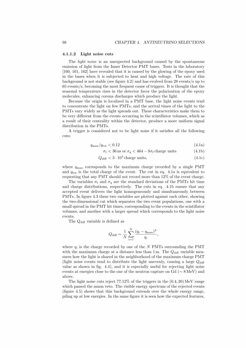
98 CHAPTER 4. ANTINEUTRINO SELECTIONS
4.1.1.2 Light noise cuts
The light noise is an unexpected background caused by the spontaneousemission of light from the Inner Detector PMT bases. Tests in the laboratory[160, 161, 162] have revealed that it is caused by the glowing of the epoxy usedin the bases when it is subjected to heat and high voltage. The rate of thisbackground is not stable (see figure 4.2) and has evolved from 28 events/s up to65 events/s, becoming the most frequent cause of triggers. It is thought that theseasonal temperature rises in the detector favor the polarization of the epoxymolecules, enhancing corona discharges which produce the light.
Because the origin is localized in a PMT base, the light noise events tendto concentrate the light on few PMTs, and the arrival times of the light to thePMTs vary widely as the light spreads out. These characteristics make them tobe very different from the events occurring in the scintillator volumes, which asa result of their centrality within the detector, produce a more uniform signaldistribution in the PMTs.
A trigger is considered not to be light noise if it satisfies all the followingcuts:
qmax/qtot < 0.12 (4.1a)σt < 36 ns or σq < 464− 8σt charge units (4.1b)
Qdiff < 3 · 104 charge units, (4.1c)
where qmax corresponds to the maximum charge recorded by a single PMTand qtot is the total charge of the event. The cut in eq. 4.1a is equivalent torequesting that any PMT should not record more than 12% of the event charge.
The variables σt and σq are the standard deviations of the PMTs hit timeand charge distributions, respectively. The cuts in eq. 4.1b ensure that anyaccepted event delivers the light homogeneously and simultaneously betweenPMTs. In figure 4.3 these two variables are plotted against each other, showingthe two-dimensional cut which separates the two event populations, one with asmall spread in the PMT hit times, corresponding to the events in the scintillatorvolumes, and another with a larger spread which corresponds to the light noiseevents.
The Qdiff variable is defined as
Qdiff =1N
N∑i=1
(qi − qmax)2
qi,
where qi is the charge recorded by one of the N PMTs surrounding the PMTwith the maximum charge at a distance less than 1 m. The Qdiff variable mea-sures how the light is shared in the neighborhood of the maximum charge PMT(light noise events tend to distribute the light unevenly, causing a large Qdiff
value as shown in fig. 4.4), and it is especially useful for rejecting light noiseevents at energies close to the one of the neutron capture on Gd (∼ 8 MeV) andabove.
The light noise cuts reject 77.12% of the triggers in the (0.4, 20) MeV rangewhich passed the muon veto. The visible energy spectrum of the rejected events(figure 4.5) shows that this background extends over the whole energy range,piling up at low energies. In the same figure it is seen how the expected features,
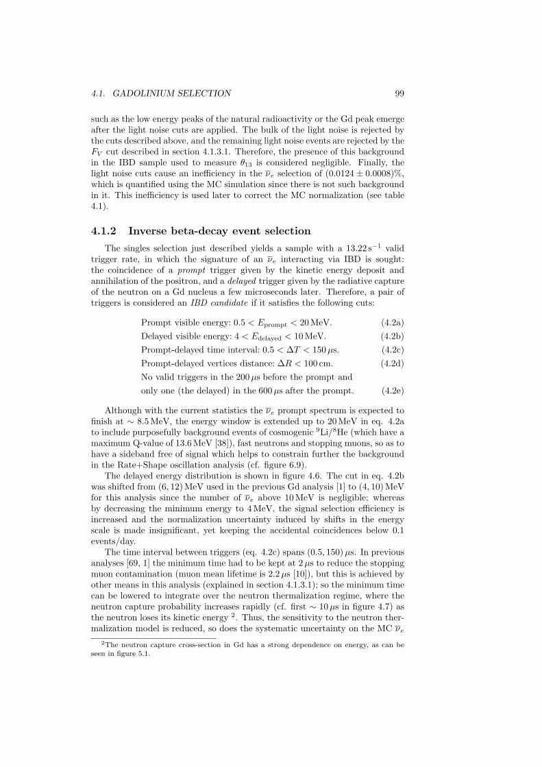
4.1. GADOLINIUM SELECTION 99
such as the low energy peaks of the natural radioactivity or the Gd peak emergeafter the light noise cuts are applied. The bulk of the light noise is rejected bythe cuts described above, and the remaining light noise events are rejected by theFV cut described in section 4.1.3.1. Therefore, the presence of this backgroundin the IBD sample used to measure θ13 is considered negligible. Finally, thelight noise cuts cause an inefficiency in the νe selection of (0.0124 ± 0.0008)%,which is quantified using the MC simulation since there is not such backgroundin it. This inefficiency is used later to correct the MC normalization (see table4.1).
4.1.2 Inverse beta-decay event selection
The singles selection just described yields a sample with a 13.22 s−1 validtrigger rate, in which the signature of an νe interacting via IBD is sought:the coincidence of a prompt trigger given by the kinetic energy deposit andannihilation of the positron, and a delayed trigger given by the radiative captureof the neutron on a Gd nucleus a few microseconds later. Therefore, a pair oftriggers is considered an IBD candidate if it satisfies the following cuts:
Prompt visible energy: 0.5 < Eprompt < 20 MeV. (4.2a)Delayed visible energy: 4 < Edelayed < 10 MeV. (4.2b)Prompt-delayed time interval: 0.5 < ∆T < 150µs. (4.2c)Prompt-delayed vertices distance: ∆R < 100 cm. (4.2d)No valid triggers in the 200µs before the prompt andonly one (the delayed) in the 600µs after the prompt. (4.2e)
Although with the current statistics the νe prompt spectrum is expected tofinish at ∼ 8.5 MeV, the energy window is extended up to 20 MeV in eq. 4.2ato include purposefully background events of cosmogenic 9Li/8He (which have amaximum Q-value of 13.6 MeV [38]), fast neutrons and stopping muons, so as tohave a sideband free of signal which helps to constrain further the backgroundin the Rate+Shape oscillation analysis (cf. figure 6.9).
The delayed energy distribution is shown in figure 4.6. The cut in eq. 4.2bwas shifted from (6, 12) MeV used in the previous Gd analysis [1] to (4, 10) MeVfor this analysis since the number of νe above 10 MeV is negligible; whereasby decreasing the minimum energy to 4 MeV, the signal selection efficiency isincreased and the normalization uncertainty induced by shifts in the energyscale is made insignificant, yet keeping the accidental coincidences below 0.1events/day.
The time interval between triggers (eq. 4.2c) spans (0.5, 150)µs. In previousanalyses [69, 1] the minimum time had to be kept at 2µs to reduce the stoppingmuon contamination (muon mean lifetime is 2.2µs [10]), but this is achieved byother means in this analysis (explained in section 4.1.3.1); so the minimum timecan be lowered to integrate over the neutron thermalization regime, where theneutron capture probability increases rapidly (cf. first ∼ 10µs in figure 4.7) asthe neutron loses its kinetic energy 2. Thus, the sensitivity to the neutron ther-malization model is reduced, so does the systematic uncertainty on the MC νe
2The neutron capture cross-section in Gd has a strong dependence on energy, as can beseen in figure 5.1.
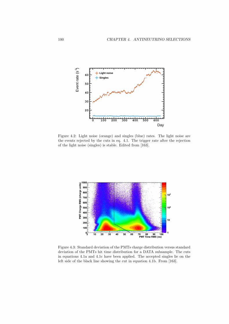
100 CHAPTER 4. ANTINEUTRINO SELECTIONS
Day0 100 200 300 400 500 600
)-1
Eve
nt r
ate
(s
20
30
40
50
60Light noise
Singles
Figure 4.2: Light noise (orange) and singles (blue) rates. The light noise arethe events rejected by the cuts in eq. 4.1. The trigger rate after the rejectionof the light noise (singles) is stable. Edited from [163].
Figure 4.3: Standard deviation of the PMTs charge distribution versus standarddeviation of the PMTs hit time distribution for a DATA subsample. The cutsin equations 4.1a and 4.1c have been applied. The accepted singles lie on theleft side of the black line showing the cut in equation 4.1b. From [163].
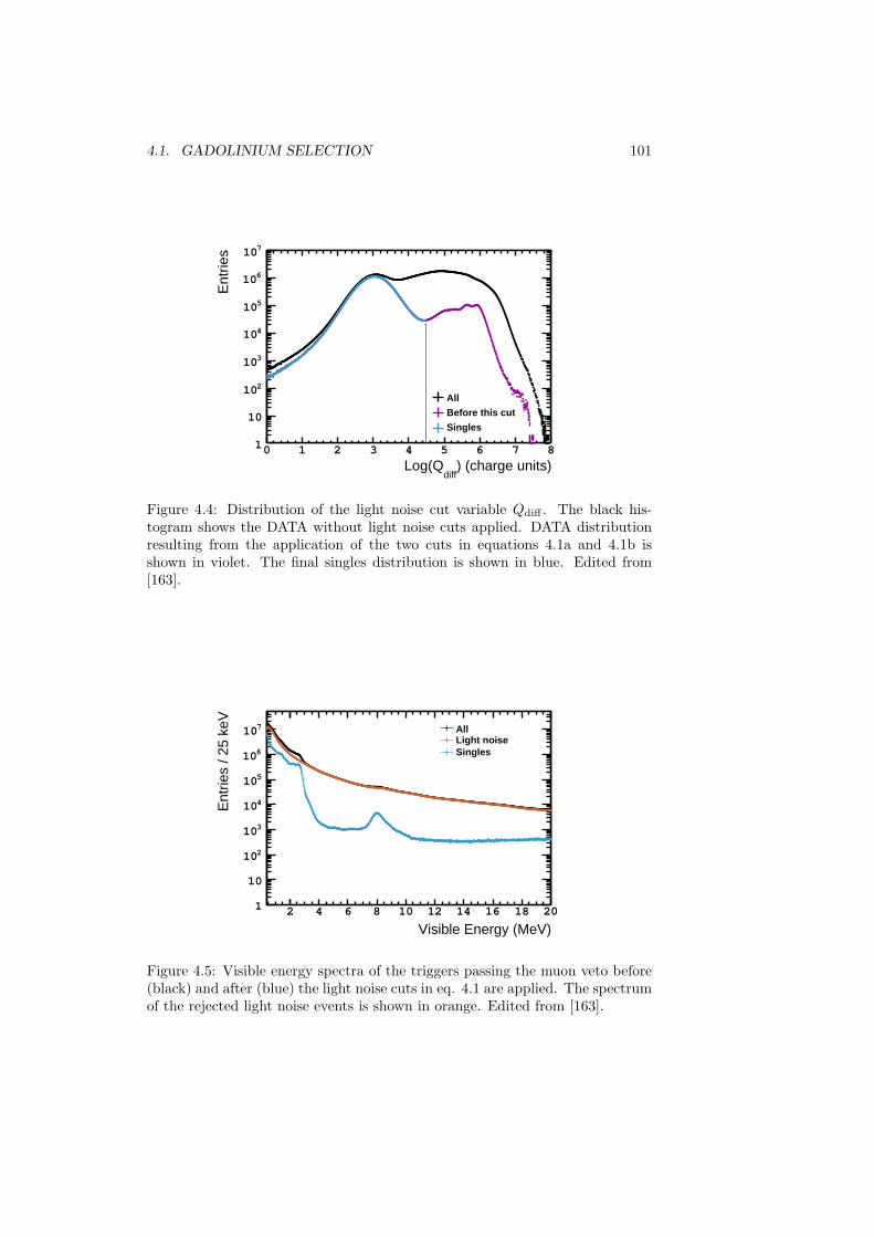
4.1. GADOLINIUM SELECTION 101
) (charge units)diff
Log(Q0 1 2 3 4 5 6 7 8
Ent
ries
1
10
210
310
410
510
610
710
All
Before this cut
Singles
Figure 4.4: Distribution of the light noise cut variable Qdiff . The black his-togram shows the DATA without light noise cuts applied. DATA distributionresulting from the application of the two cuts in equations 4.1a and 4.1b isshown in violet. The final singles distribution is shown in blue. Edited from[163].
Visible Energy (MeV)2 4 6 8 10 12 14 16 18 20
Ent
ries
/ 25
keV
1
10
210
310
410
510
610
710 AllLight noiseSingles
Figure 4.5: Visible energy spectra of the triggers passing the muon veto before(black) and after (blue) the light noise cuts in eq. 4.1 are applied. The spectrumof the rejected light noise events is shown in orange. Edited from [163].
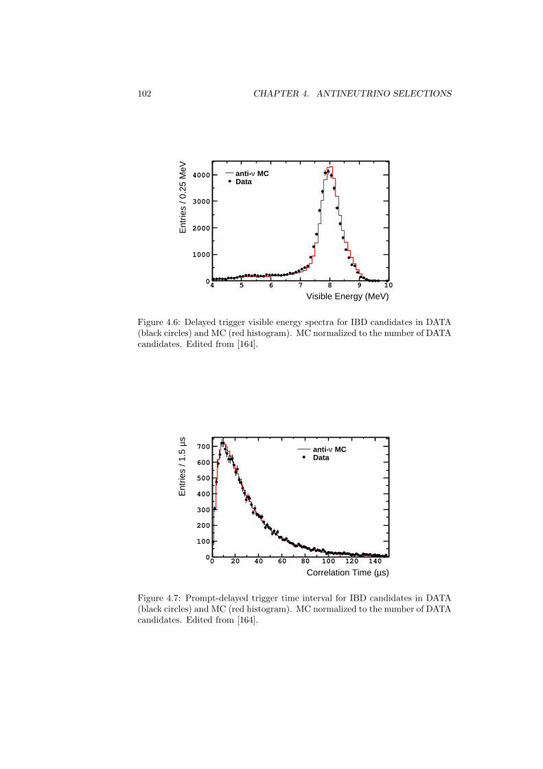
102 CHAPTER 4. ANTINEUTRINO SELECTIONS
Visible Energy (MeV)4 5 6 7 8 9 10
Ent
ries
/ 0.2
5 M
eV
0
1000
2000
3000
4000 MCνanti-
Data
MCνanti-Data
Figure 4.6: Delayed trigger visible energy spectra for IBD candidates in DATA(black circles) and MC (red histogram). MC normalized to the number of DATAcandidates. Edited from [164].
s)µCorrelation Time (0 20 40 60 80 100 120 140
sµE
ntrie
s / 1
.5
0
100
200
300
400
500
600
700 MCνanti-Data
Figure 4.7: Prompt-delayed trigger time interval for IBD candidates in DATA(black circles) and MC (red histogram). MC normalized to the number of DATAcandidates. Edited from [164].
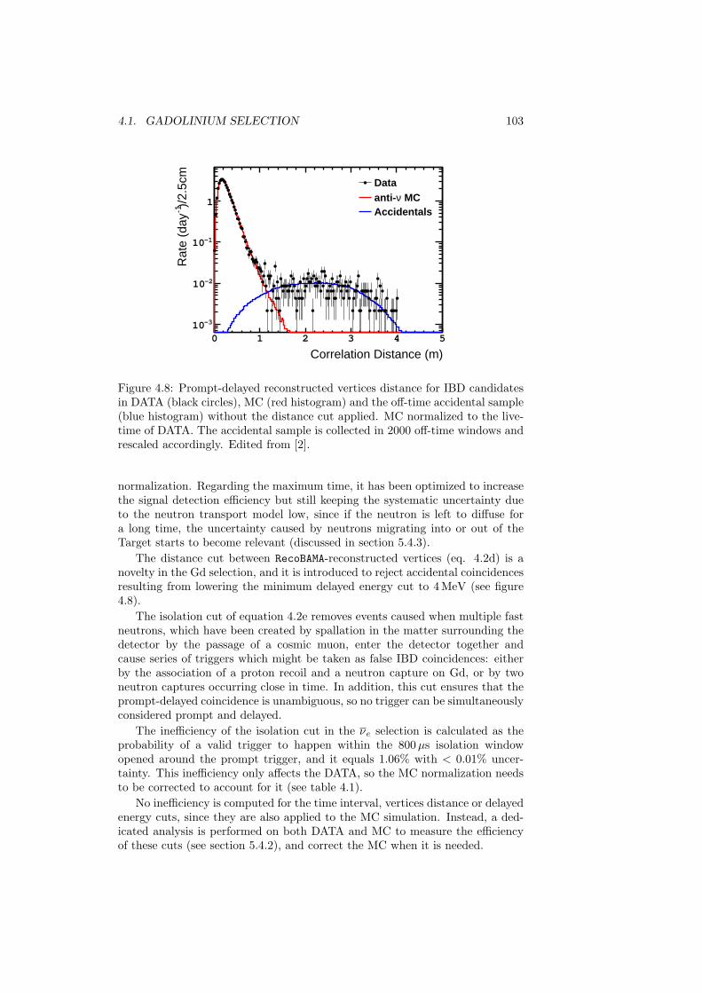
4.1. GADOLINIUM SELECTION 103
Correlation Distance (m)0 1 2 3 4 5
)/2.
5cm
-1R
ate
(day
-310
-210
-110
1
Data MCνanti-
Accidentals
Figure 4.8: Prompt-delayed reconstructed vertices distance for IBD candidatesin DATA (black circles), MC (red histogram) and the off-time accidental sample(blue histogram) without the distance cut applied. MC normalized to the live-time of DATA. The accidental sample is collected in 2000 off-time windows andrescaled accordingly. Edited from [2].
normalization. Regarding the maximum time, it has been optimized to increasethe signal detection efficiency but still keeping the systematic uncertainty dueto the neutron transport model low, since if the neutron is left to diffuse fora long time, the uncertainty caused by neutrons migrating into or out of theTarget starts to become relevant (discussed in section 5.4.3).
The distance cut between RecoBAMA-reconstructed vertices (eq. 4.2d) is anovelty in the Gd selection, and it is introduced to reject accidental coincidencesresulting from lowering the minimum delayed energy cut to 4 MeV (see figure4.8).
The isolation cut of equation 4.2e removes events caused when multiple fastneutrons, which have been created by spallation in the matter surrounding thedetector by the passage of a cosmic muon, enter the detector together andcause series of triggers which might be taken as false IBD coincidences: eitherby the association of a proton recoil and a neutron capture on Gd, or by twoneutron captures occurring close in time. In addition, this cut ensures that theprompt-delayed coincidence is unambiguous, so no trigger can be simultaneouslyconsidered prompt and delayed.
The inefficiency of the isolation cut in the νe selection is calculated as theprobability of a valid trigger to happen within the 800µs isolation windowopened around the prompt trigger, and it equals 1.06% with < 0.01% uncer-tainty. This inefficiency only affects the DATA, so the MC normalization needsto be corrected to account for it (see table 4.1).
No inefficiency is computed for the time interval, vertices distance or delayedenergy cuts, since they are also applied to the MC simulation. Instead, a ded-icated analysis is performed on both DATA and MC to measure the efficiencyof these cuts (see section 5.4.2), and correct the MC when it is needed.
104 CHAPTER 4. ANTINEUTRINO SELECTIONS
4.1.3 Background vetoes and estimations
After the search for IBD-like coincidences using the cuts in equations 4.2, thesurviving backgrounds are processes capable of mimicking the IBD interactionsignature. Among these, the main causes are the accidental coincidence of twouncorrelated triggers or the coincidence of two correlated triggers caused by fastneutrons, stopping muons or some cosmogenic isotopes. All these sources aredescribed in what follows, adding how their rates and prompt energy spectra canbe estimated. Moreover, the ones which cause correlated triggers are originatedby the interaction of cosmic muons with matter. For them, a series of vetoesare applied in order to further reduce the background contamination.
4.1.3.1 Fast neutrons and stopping muons
These two backgrounds are capable of causing trigger coincidences whichresemble the IBD interaction. The rate of these fake IBD coincidences can bedecreased by using the subdetectors which provide active background rejection(OV and IV) as vetoes or by using the trigger charge-hit time PMT information(FV veto).
The fast neutrons are high energy neutrons entering the detector (meankinetic energy ∼ 20 MeV [66]), which have been produced by muon-inducedspallation of the nuclei in the rock surrounding the detector. Since the muonis missed by the Inner Detector and the Inner Veto, it does not fire the muonveto. The prompt trigger is given by a neutron interacting with a proton inthe Target or Gamma Catcher scintillator volumes, causing it to recoil. Thedelayed trigger is given by the radiative capture on Gd of one of the neutrons(not necessarily the one which caused the proton recoil) after it has thermalized.
The stopping muons are muons which stop inside the detector. If the energydeposited is low enough (Evis < 20 MeV), they do not fire the muon veto andare mistaken as prompt triggers. The delayed trigger is given by the Michelelectron/positron created when the muon decays:
µ− → e−νeνµ, µ+ → e+νeνµ.
OV veto
The Outer Veto is a muon-oriented subdetector (see section 2.3.2) which sitson top of the main detector and which extends beyond the area occupied by it;so it is capable of detecting impinging muons, including those which do not gothrough the detector but pass close by it. Any IBD candidate whose prompttrigger is coincident with an OV trigger is discarded (because of the differenttiming in the Inner Detector and the Outer veto, coincident is defined as “within224 ns”).
The dead-time introduced by this veto is estimated using a fixed rate trigger.Counting the number of those triggers which are coincident with an OV triggergives a (0.058± 0.001)% inefficiency in the νe selection due to the OV veto.
IV veto
Any particle (fast neutrons, stopping muons, but also γ-rays) entering thedetector from outside will have to cross the Inner Veto on its way to the Inner
4.1. GADOLINIUM SELECTION 105
Detector, so there is a chance that it will leave part of its energy in the InnerVeto, yet below the muon veto threshold. Therefore, any prompt trigger whichshows a certain coincident activity in the Inner Veto is considered to be causedby an incoming background particle and rejected. All the following conditionsmust be fulfilled to execute this veto:
IV PMT hit multiplicity ≥ 2 (4.3a)Total charge in the IV > 400 charge units (≈ 0.2 MeV) (4.3b)ID-IV vertices distance < 3.7 m (4.3c)ID-IV time interval: − 110 < ∆TID−IV < −10 ns. (4.3d)
The cuts above are tuned to reduce the background while keeping the rejectionof νe due to accidental Inner Detector-Inner Veto coincidences low (see figure4.9). This is predominantly achieved by requiring both time (eq. 4.3d) andspatial (eq. 4.3c) coincidences; where the reconstructed vertex in the Inner Vetois obtained from an artificial neural network which uses as inputs the relativenumbers of photoelectrons in each Inner Veto PMT with respect to the totalnumber of photoelectrons observed by the 78 Inner Veto PMTs.
The inefficiency in the νe selection because of the IV veto is estimated tobe (0.035±0.014)% from the fraction of accidental candidates selected with theoff-time method (section 4.1.3.3) which are rejected by the IV veto.
No veto is applied on the delayed trigger since the deexcitation γ rays emittedupon the radiative neutron capture on Gd reach the Inner Veto with a non-negligible rate; which would lead to an excessive rejection of νe interactions.
FV veto
The chimney used to fill the Target and Gamma Catcher volumes containsliquid scintillator, so any muon entering through it will produce scintillationlight which can cause a trigger. Moreover, it is not protected by the Inner Veto,and despite the Upper Outer Veto being designed to cover it, 72.4% of the DATAwere taken without the Upper Outer Veto operative. Therefore, it is a naturalentrance of stopping muons. In order to reject those events, a veto based onthe delayed trigger FV , the negative log-likelihood of the event reconstruction(equation 3.13) was devised,
Edelayed < 0.068 exp(FV /1.23), (4.4)
exploiting the fact that FV shows a high value for events with a hit pattern notcompatible with a point-like source in the Target or the Gamma Catcher, suchas the chimney stopping muons or the light noise events which survived the cutsin eqs. 4.1.
In figure 4.10 it is shown how the cut in equation 4.4 separates the IBDcandidates (the left distribution) from the background events, which do notexhibit clustering around the Gd neutron capture energy. By looking at thevertex distribution in figure 4.11, it is observed how the rejected events pileup below the chimney (stopping muons) or in the center of the detector (mis-reconstructed light noise). This is further confirmed by examining the prompt-delayed time distribution of the rejected events (cf. figure 4.12), which shows afast decay time constant which is characteristic of the decay of stopped muonsor a prolonged light noise emission which gives two consecutive triggers.
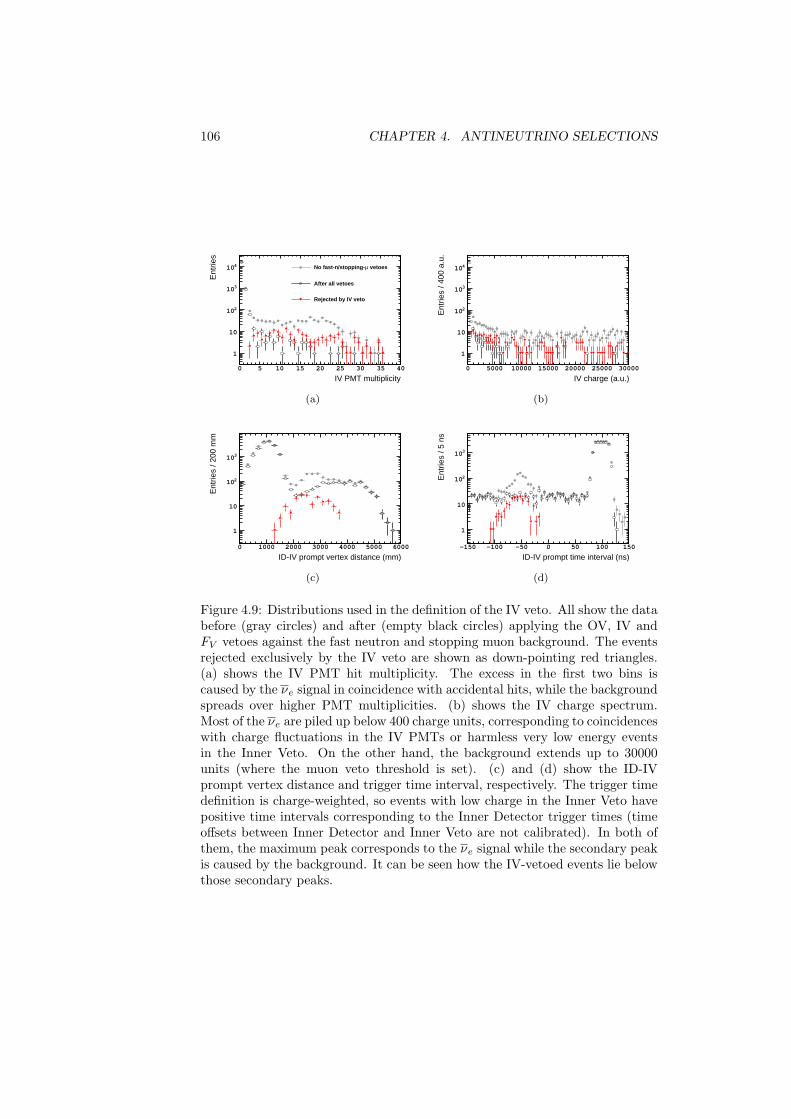
106 CHAPTER 4. ANTINEUTRINO SELECTIONS
IV PMT multiplicity0 5 10 15 20 25 30 35 40
Ent
ries
1
10
210
310
410 vetoesµNo fast-n/stopping-
After all vetoes
Rejected by IV veto
(a)
IV charge (a.u.)0 5000 10000 15000 20000 25000 30000
Ent
ries
/ 400
a.u
.
1
10
210
310
410
(b)
ID-IV prompt vertex distance (mm)0 1000 2000 3000 4000 5000 6000
Ent
ries
/ 200
mm
1
10
210
310
(c)
ID-IV prompt time interval (ns)-150 -100 -50 0 50 100 150
Ent
ries
/ 5 n
s
1
10
210
310
(d)
Figure 4.9: Distributions used in the definition of the IV veto. All show the databefore (gray circles) and after (empty black circles) applying the OV, IV andFV vetoes against the fast neutron and stopping muon background. The eventsrejected exclusively by the IV veto are shown as down-pointing red triangles.(a) shows the IV PMT hit multiplicity. The excess in the first two bins iscaused by the νe signal in coincidence with accidental hits, while the backgroundspreads over higher PMT multiplicities. (b) shows the IV charge spectrum.Most of the νe are piled up below 400 charge units, corresponding to coincidenceswith charge fluctuations in the IV PMTs or harmless very low energy eventsin the Inner Veto. On the other hand, the background extends up to 30000units (where the muon veto threshold is set). (c) and (d) show the ID-IVprompt vertex distance and trigger time interval, respectively. The trigger timedefinition is charge-weighted, so events with low charge in the Inner Veto havepositive time intervals corresponding to the Inner Detector trigger times (timeoffsets between Inner Detector and Inner Veto are not calibrated). In both ofthem, the maximum peak corresponds to the νe signal while the secondary peakis caused by the background. It can be seen how the IV-vetoed events lie belowthose secondary peaks.
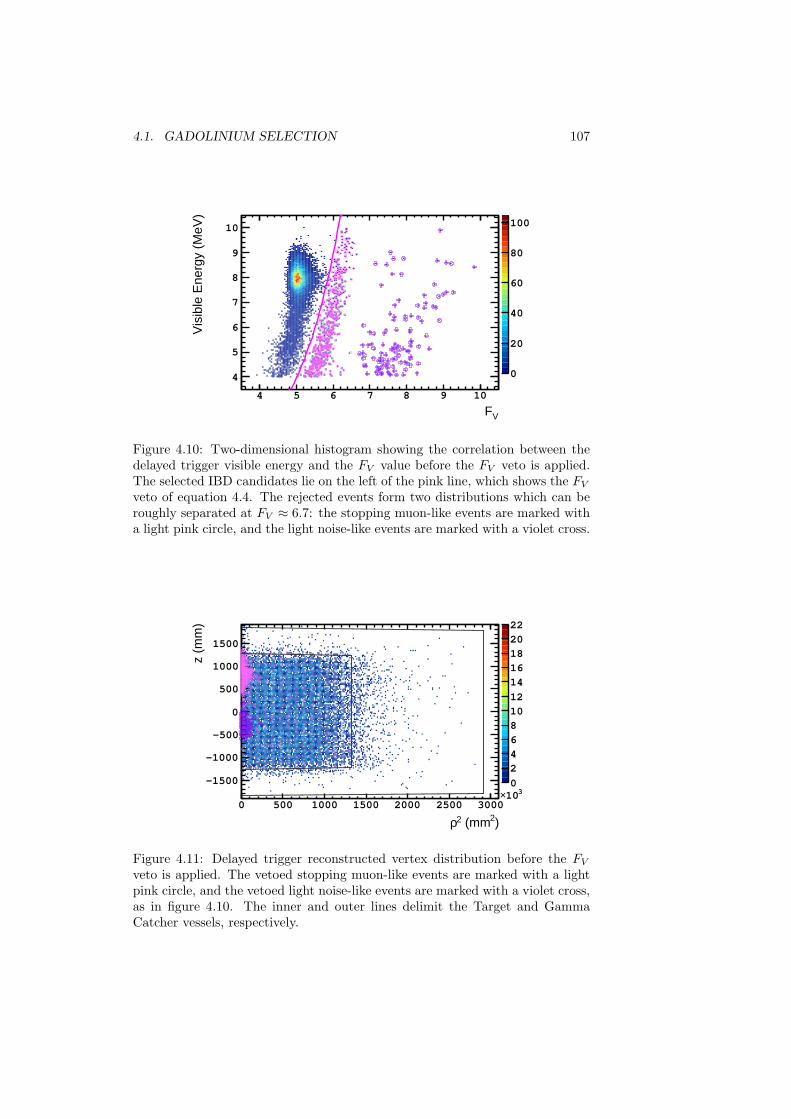
4.1. GADOLINIUM SELECTION 107
V F4 5 6 7 8 9 10
Vis
ible
Ene
rgy
(MeV
)
4
5
6
7
8
9
10
0
20
40
60
80
100
Figure 4.10: Two-dimensional histogram showing the correlation between thedelayed trigger visible energy and the FV value before the FV veto is applied.The selected IBD candidates lie on the left of the pink line, which shows the FVveto of equation 4.4. The rejected events form two distributions which can beroughly separated at FV ≈ 6.7: the stopping muon-like events are marked witha light pink circle, and the light noise-like events are marked with a violet cross.
)2 (mm2ρ0 500 1000 1500 2000 2500 3000
310×
z (m
m)
-1500
-1000
-500
0
500
1000
1500
Ent
ries
0
2
4
6
8
10
12
14
16
18
20
22
Figure 4.11: Delayed trigger reconstructed vertex distribution before the FVveto is applied. The vetoed stopping muon-like events are marked with a lightpink circle, and the vetoed light noise-like events are marked with a violet cross,as in figure 4.10. The inner and outer lines delimit the Target and GammaCatcher vessels, respectively.
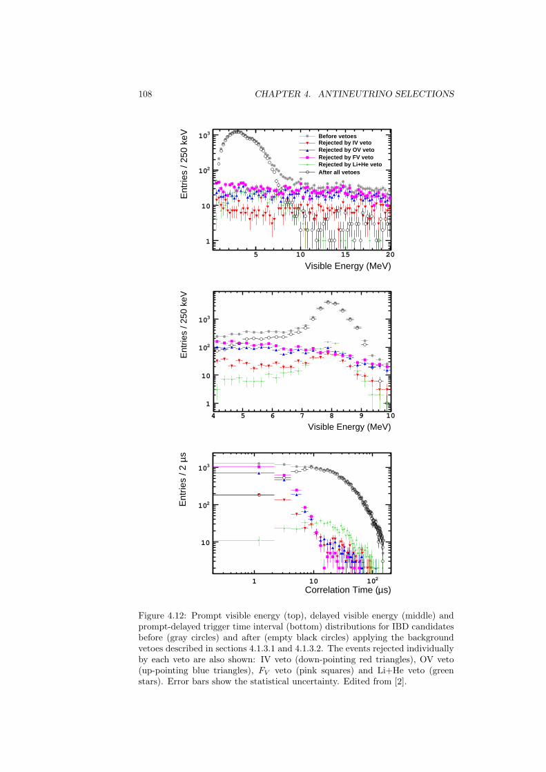
108 CHAPTER 4. ANTINEUTRINO SELECTIONS
Visible Energy (MeV)5 10 15 20
Ent
ries
/ 250
keV
1
10
210
310 Before vetoesRejected by IV vetoRejected by OV vetoRejected by FV vetoRejected by Li+He vetoAfter all vetoes
Visible Energy (MeV)4 5 6 7 8 9 10
Ent
ries
/ 250
keV
1
10
210
310
s)µCorrelation Time (1 10 210
sµE
ntrie
s / 2
10
210
310
Figure 4.12: Prompt visible energy (top), delayed visible energy (middle) andprompt-delayed trigger time interval (bottom) distributions for IBD candidatesbefore (gray circles) and after (empty black circles) applying the backgroundvetoes described in sections 4.1.3.1 and 4.1.3.2. The events rejected individuallyby each veto are also shown: IV veto (down-pointing red triangles), OV veto(up-pointing blue triangles), FV veto (pink squares) and Li+He veto (greenstars). Error bars show the statistical uncertainty. Edited from [2].
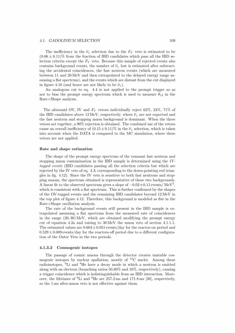
4.1. GADOLINIUM SELECTION 109
The inefficiency in the νe selection due to the FV veto is estimated to be(0.06 ± 0.11)% from the fraction of IBD candidates which pass all the IBD se-lection criteria except the FV veto. Because this sample of rejected events alsocontains background events, the number of νe lost is estimated after subtract-ing the accidental coincidences, the fast neutron events (which are measuredbetween 11 and 20 MeV and then extrapolated to the delayed energy range as-suming a flat spectrum), and the events which are distant from the cut displayedin figure 4.10 (and hence are not likely to be νe).
An analogous cut to eq. 4.4 is not applied to the prompt trigger so asnot to bias the prompt energy spectrum which is used to measure θ13 in theRate+Shape analysis.
The aforesaid OV, IV and FV vetoes individually reject 62%, 24%, 71% ofthe IBD candidates above 12 MeV, respectively, where νe are not expected andthe fast neutron and stopping muon background is dominant. When the threevetoes act together, a 90% rejection is obtained. The combined use of the vetoescause an overall inefficiency of (0.15± 0.11)% in the νe selection, which is takeninto account when the DATA is compared to the MC simulation, where thesevetoes are not applied.
Rate and shape estimation
The shape of the prompt energy spectrum of the remnant fast neutron andstopping muon contamination in the IBD sample is determined using the IV-tagged events (IBD candidates passing all the selection criteria but which arerejected by the IV veto of eq. 4.3; corresponding to the down-pointing red trian-gles in fig. 4.12). Since the IV veto is sensitive to both fast neutrons and stop-ping muons, the spectrum obtained is representative of these two backgrounds.A linear fit to the observed spectrum gives a slope of −0.02±0.11 events/MeV2,which is consistent with a flat spectrum. This is further confirmed by the shapesof the OV-tagged events and the remaining IBD candidates beyond 12 MeV inthe top plot of figure 4.12. Therefore, this background is modeled as flat in theRate+Shape oscillation analysis.
The rate of the background events still present in the IBD sample is ex-trapolated assuming a flat spectrum from the measured rate of coincidencesin the range (20, 30) MeV, which are obtained modifying the prompt energycut of equation 4.2a and raising to 30 MeV the muon veto of section 4.1.1.1.The estimated values are 0.604±0.051 events/day for the reactor-on period and0.529± 0.089 events/day for the reactors-off period due to a different configura-tion of the Outer Veto in the two periods.
4.1.3.2 Cosmogenic isotopes
The passage of cosmic muons through the detector creates unstable cos-mogenic isotopes by nuclear spallation, mostly of 12C nuclei. Among theseradioisotopes, 9Li and 8He have a decay mode in which a neutron is emittedalong with an electron (branching ratios 50.80% and 16%, respectively), causinga trigger coincidence which is indistinguishable from an IBD interaction. More-over, the lifetimes of 9Li and 8He are 257.2 ms and 171.8 ms [38], respectively,so the 1 ms after-muon veto is not effective against them.
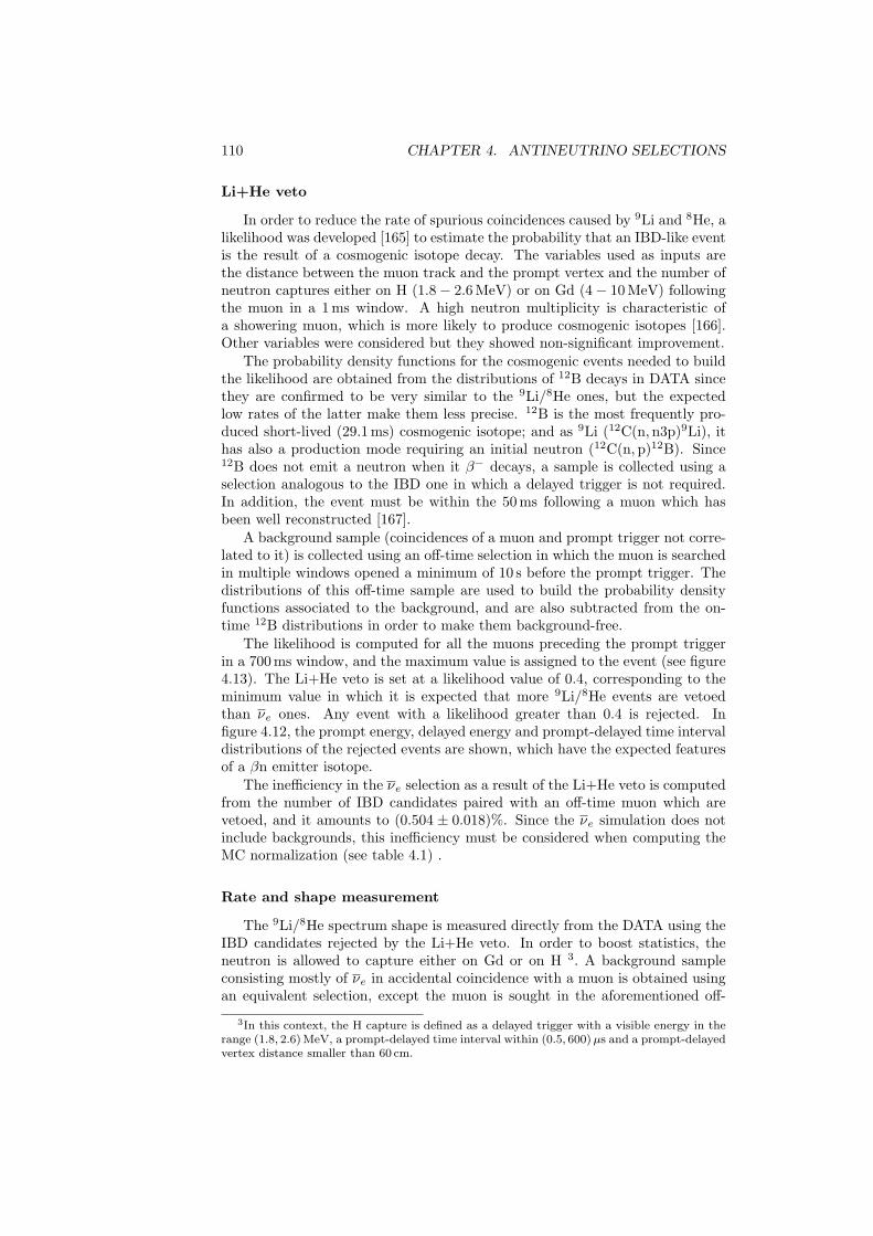
110 CHAPTER 4. ANTINEUTRINO SELECTIONS
Li+He veto
In order to reduce the rate of spurious coincidences caused by 9Li and 8He, alikelihood was developed [165] to estimate the probability that an IBD-like eventis the result of a cosmogenic isotope decay. The variables used as inputs arethe distance between the muon track and the prompt vertex and the number ofneutron captures either on H (1.8− 2.6 MeV) or on Gd (4− 10 MeV) followingthe muon in a 1 ms window. A high neutron multiplicity is characteristic ofa showering muon, which is more likely to produce cosmogenic isotopes [166].Other variables were considered but they showed non-significant improvement.
The probability density functions for the cosmogenic events needed to buildthe likelihood are obtained from the distributions of 12B decays in DATA sincethey are confirmed to be very similar to the 9Li/8He ones, but the expectedlow rates of the latter make them less precise. 12B is the most frequently pro-duced short-lived (29.1 ms) cosmogenic isotope; and as 9Li (12C(n,n3p)9Li), ithas also a production mode requiring an initial neutron (12C(n,p)12B). Since12B does not emit a neutron when it β− decays, a sample is collected using aselection analogous to the IBD one in which a delayed trigger is not required.In addition, the event must be within the 50 ms following a muon which hasbeen well reconstructed [167].
A background sample (coincidences of a muon and prompt trigger not corre-lated to it) is collected using an off-time selection in which the muon is searchedin multiple windows opened a minimum of 10 s before the prompt trigger. Thedistributions of this off-time sample are used to build the probability densityfunctions associated to the background, and are also subtracted from the on-time 12B distributions in order to make them background-free.
The likelihood is computed for all the muons preceding the prompt triggerin a 700 ms window, and the maximum value is assigned to the event (see figure4.13). The Li+He veto is set at a likelihood value of 0.4, corresponding to theminimum value in which it is expected that more 9Li/8He events are vetoedthan νe ones. Any event with a likelihood greater than 0.4 is rejected. Infigure 4.12, the prompt energy, delayed energy and prompt-delayed time intervaldistributions of the rejected events are shown, which have the expected featuresof a βn emitter isotope.
The inefficiency in the νe selection as a result of the Li+He veto is computedfrom the number of IBD candidates paired with an off-time muon which arevetoed, and it amounts to (0.504 ± 0.018)%. Since the νe simulation does notinclude backgrounds, this inefficiency must be considered when computing theMC normalization (see table 4.1) .
Rate and shape measurement
The 9Li/8He spectrum shape is measured directly from the DATA using theIBD candidates rejected by the Li+He veto. In order to boost statistics, theneutron is allowed to capture either on Gd or on H 3. A background sampleconsisting mostly of νe in accidental coincidence with a muon is obtained usingan equivalent selection, except the muon is sought in the aforementioned off-
3In this context, the H capture is defined as a delayed trigger with a visible energy in therange (1.8, 2.6) MeV, a prompt-delayed time interval within (0.5, 600)µs and a prompt-delayedvertex distance smaller than 60 cm.
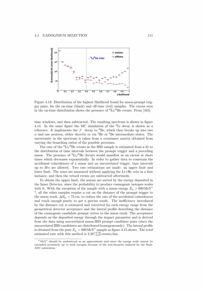
4.1. GADOLINIUM SELECTION 111
Likelihood0 0.1 0.2 0.3 0.4 0.5 0.6 0.7 0.8 0.9 1
En
trie
s/(0
.04
un
its
likel
iho
od
)
1
10
210
310
410 ontime
offtimeHe Veto8Li/9 →
Double Chooz Preliminary
Figure 4.13: Distribution of the highest likelihood found for muon-prompt trig-ger pairs, for the on-time (black) and off-time (red) samples. The excess seenin the on-time distribution shows the presence of 9Li/8He events. From [165].
time windows, and then subtracted. The resulting spectrum is shown in figure4.14. In the same figure the MC simulation of the 9Li decay is shown as areference. It implements the β− decay to 9Be, which then breaks up into twoα and one neutron, either directly or via 5He or 8Be intermediate states. Theuncertainty in the spectrum is taken from a covariance matrix obtained fromvarying the branching ratios of the possible processes.
The rate of the 9Li/8He events in the IBD sample is estimated from a fit tothe distribution of time intervals between the prompt trigger and a precedingmuon. The presence of 9Li/8He decays would manifest as an excess at shorttimes which decreases exponentially. In order to gather data to constrain theaccidental coincidences of a muon and an uncorrelated trigger, time intervalsup to 20 s are allowed. Two rate estimations are made: an upper limit andlower limit. The rates are measured without applying the Li+He veto in a firstinstance, and then the vetoed events are subtracted afterwards.
To obtain the upper limit, the muons are sorted by the energy deposited inthe Inner Detector, since the probability to produce cosmogenic isotopes scaleswith it. With the exception of the sample with a muon energy Eµ > 600 MeV∗4, all the other samples require a cut on the distance of the prompt trigger tothe muon track, ∆Rµ < 75 cm, to reduce the rate of the accidental coincidencesand reach enough purity to get a precise result. The inefficiency introducedby the distance cut is estimated and corrected for each energy range from thegeometrical detector acceptance and the lateral profile describing the distanceof the cosmogenic candidate prompt vertex to the muon track. The acceptancedepends on the deposited energy through the impact parameter and is derivedfrom the data using uncorrelated muon-IBD prompt candidate pairs (since theuncorrelated IBD candidates are distributed homogeneously). The lateral profileis obtained from the pure Eµ > 600 MeV∗ sample as figure 4.15 shows. The totalestimated rate with this method is 2.20+0.35
−0.27 events/day.
4 MeV∗ should be understood as an approximate unit since the energy scale cannot beextended accurately up to such energies because of the non-linearity induced by the flash-ADC saturation.
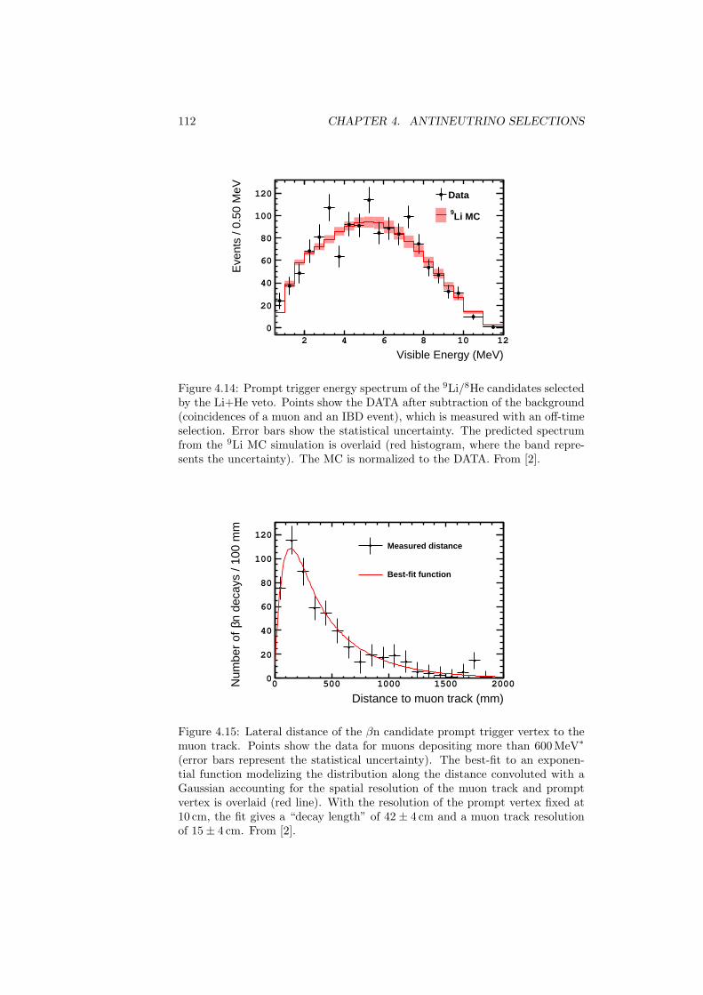
112 CHAPTER 4. ANTINEUTRINO SELECTIONS
Visible Energy (MeV)2 4 6 8 10 12
Eve
nts
/ 0.5
0 M
eV
0
20
40
60
80
100
120 Data
Li MC9
Figure 4.14: Prompt trigger energy spectrum of the 9Li/8He candidates selectedby the Li+He veto. Points show the DATA after subtraction of the background(coincidences of a muon and an IBD event), which is measured with an off-timeselection. Error bars show the statistical uncertainty. The predicted spectrumfrom the 9Li MC simulation is overlaid (red histogram, where the band repre-sents the uncertainty). The MC is normalized to the DATA. From [2].
Distance to muon track (mm)0 500 1000 1500 2000
n de
cays
/ 10
0 m
mβ
Num
ber
of
0
20
40
60
80
100
120Measured distance
Best-fit function
Figure 4.15: Lateral distance of the βn candidate prompt trigger vertex to themuon track. Points show the data for muons depositing more than 600 MeV∗
(error bars represent the statistical uncertainty). The best-fit to an exponen-tial function modelizing the distribution along the distance convoluted with aGaussian accounting for the spatial resolution of the muon track and promptvertex is overlaid (red line). With the resolution of the prompt vertex fixed at10 cm, the fit gives a “decay length” of 42 ± 4 cm and a muon track resolutionof 15± 4 cm. From [2].
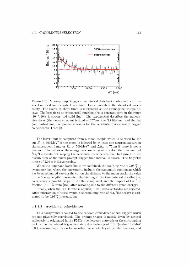
4.1. GADOLINIUM SELECTION 113
T (ms)∆0 500 1000 1500 2000
Ent
ries
/ 20
ms
0
20
40
60
80
100
120
140
160
180
200
He enriched data8Li/9
Best-fit function
Figure 4.16: Muon-prompt trigger time interval distribution obtained with theselection used for the rate lower limit. Error bars show the statistical uncer-tainty. The excess at short times is interpreted as the cosmogenic isotope de-cays. The best-fit to an exponential function plus a constant term in the range[10−3, 20] s is shown (red solid line). The exponential describes the radioac-tive decay (the decay constant is fixed at 257 ms, the 9Li lifetime) and the flat(red dashed line) component accounts for the accidental muon-prompt triggercoincidences. From [2].
The lower limit is computed from a muon sample which is selected by thecut Eµ > 300 MeV∗ if the muon is followed by at least one neutron capture inthe subsequent 1 ms, or Eµ > 500 MeV∗ and ∆Rµ < 75 cm if there is not aneutron. The values of the energy cuts are targeted to select the maximum of9Li/8He events but keeping the accidental coincidences low. In figure 4.16 thedistribution of the muon-prompt trigger time interval is shown. The fit yieldsa rate of 2.05± 0.13 events/day.
When the upper and lower limits are combined, the resulting rate is 2.08+0.41−0.15
events per day, where the uncertainty includes the systematic component whichhas been estimated varying the cut on the distance to the muon track, the valueof the “decay length” parameter, the binning in the time interval distribution,considering a possible slope in the flat component and the impact of the 8Hefraction (8± 7% from [166] after rescaling due to the different muon energy).
Finally, when the Li+He veto is applied, 1.12±0.05 events/day are rejected.After subtraction of those events, the remaining rate of 9Li/8He decays is esti-mated to be 0.97+0.41
−0.16 events/day.
4.1.3.3 Accidental coincidences
This background is caused by the random coincidence of two triggers whichare not physically correlated. The prompt trigger is mostly given by naturalradioactivity originated in the PMTs, the detector materials or the surroundingrock; while the delayed trigger is mainly due to decays of 12B (Q-value 13.4 MeV[38]), neutron captures on Gd or other nuclei which yield similar energies, and
114 CHAPTER 4. ANTINEUTRINO SELECTIONS
proton recoils.Because of its random origin, this background can be measured directly from
the DATA by applying the same selection cuts in eq. 4.2 and background vetoesof sections 4.1.3.1 and 4.1.3.2, except for the prompt-delayed time interval cut(eq. 4.2c), which is substituted by:
(0.5µs + Toff) < ∆T < (150µs + Toff) (4.5)
where Toff is a time offset which must be chosen long enough so as to guaranteethat no correlation exists between the two triggers. In addition, because the twotriggers are widely separated in time, the isolation cut in equation 4.2e must bereplaced by two cuts:
No valid triggers in the 200µs beforeand in the 600µs after the prompt. (4.6a)No valid triggers in the 200µs before the time tprompt + Toff
and only one (the delayed) in the 600µs after it. (4.6b)
where tprompt is the prompt trigger time.The time offset is given by the formula:
Toff = 1 s + n× Tiso (4.7)
where Tiso = 800µs is the length of the isolation window of equation 4.2e and nis an integer in the interval [0, 1999]. The minimum offset is 1 s, which ensuresonly uncorrelated triggers are considered. The use of 2000 consecutive timewindows allows to increase the statistics of this background to have a moreprecise measurement.
The technique to measure the accidental background from the DATA justdescribed is known as the off-time method. It provides the rate and the spectrumof the accidental background for the off-time sample defined by equation 4.5.However, in order to have a measurement corresponding to the on-time sampledefined by equation 4.2c, the off-time results must be corrected to account forthe different effect that some of the cuts have in the two samples.
Muon veto correction From section 4.1.1.1 it is understood that, in orderto consider a trigger valid, the 1 ms preceding it must be free of triggers taggedas muons. Whereas the probability of having a prompt trigger vetoed by amuon is the same in the on-time and off-time samples, the delayed one is not.In the on-time sample, the proximity in time required for the delayed triggerresults in the muon-free 1 ms windows before the prompt and delayed triggersbeing mostly overlapped; whereas in the off-time sample the muon-free windowsbefore the prompt and delayed triggers do not overlap at all, thus increasingthe probability of vetoing the delayed with respect to the on-time case.
The resulting underestimation is corrected using a correction factor, fµ,which is calculated as the ratio of the Poissonian probabilities of non-vetoingthe delayed trigger (i.e. having 0 muons before it) in the on-time and off-timesamples, P on
µ and P offµ , respectively; once the vetoed events in which the muon
occurs before the prompt trigger are removed:
fµ =P onµ
P offµ
(4.8a)
4.1. GADOLINIUM SELECTION 115
with
P onµ =
∆Tmax∫∆Tmin
e−Rµt′dt′
∆Tmax∫∆Tmin
dt′
(4.8b)
P offµ = e−RµTµ (4.8c)
where Rµ is the rate of the muon-tagged events and Tµ = 1 ms is the lengthof the muon veto window. P on
µ corresponds to the averaged probability in thetime interval from equation 4.2c, so the integral limits are ∆Tmin = 0.5µs and∆Tmax = 150µs. Computing the expressions in eqs. 4.8 gives fµ = 1.04272 ±0.00002.
Isolation cut correction In the on-time sample only one isolation cut isapplied (eq. 4.2e) whereas in the off-time sample two cuts are used (eqs. 4.6aand 4.6b). Therefore, there is an additional inefficiency in the off-time samplewhich must be corrected. The correction factor, fiso, is computed as the ratioof the probabilities in the on-time and off-time samples of the delayed trigger,d, passing the isolation cut provided that the prompt trigger, p, has passed theisolation cut:
fiso =P on(d is isolated|p is isolated)P off(d is isolated|p is isolated)
(4.9)
In the on-time sample, no additional isolation cut is requested for the delayed,so P on(d is isolated|p is isolated) = 1. In the off-time sample, the probability isgiven by:
P off(d is isolated|p is isolated) = e−RsTiso + h(Rs, Tiso, Rµ, Tµ,∆T ) (4.10)
where Rs is the singles rate. The first term in 4.10 corresponds to the Poissonprobability of having 0 additional valid triggers in the isolation window coveringthe delayed trigger. The second term is a correction to the previous one whichmust be computed numerically (see [168] for the computation) and which ac-counts for the case in which there is a preceding trigger which would make thedelayed fail the isolation cut, but this preceding trigger has been removed fromthe sample by the muon veto. The value of fiso is found to be 1.0106± 0.0002.
Run length correction In the off-time method, the trigger coincidences aresearched within multiple time windows shifted by a time offset Toff . Hence,the live-time in which those coincidences can be found is reduced with respectto the on-time coincidences, since the last seconds of each run produce lesscoincidences because the time windows cannot be opened beyond the end of therun. This is corrected using the following correction factor:
frun =T run
T run − T off
(4.11)
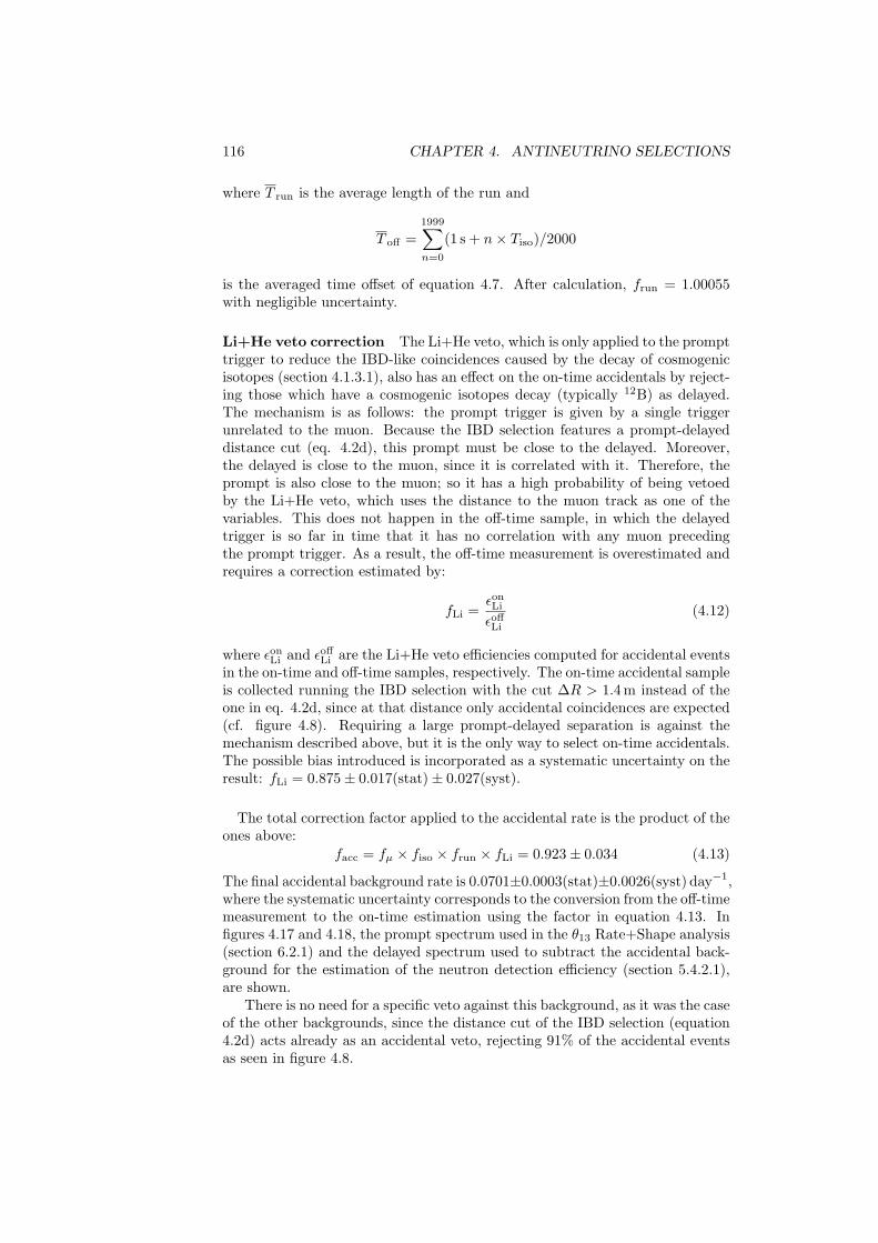
116 CHAPTER 4. ANTINEUTRINO SELECTIONS
where T run is the average length of the run and
T off =1999∑n=0
(1 s + n× Tiso)/2000
is the averaged time offset of equation 4.7. After calculation, frun = 1.00055with negligible uncertainty.
Li+He veto correction The Li+He veto, which is only applied to the prompttrigger to reduce the IBD-like coincidences caused by the decay of cosmogenicisotopes (section 4.1.3.1), also has an effect on the on-time accidentals by reject-ing those which have a cosmogenic isotopes decay (typically 12B) as delayed.The mechanism is as follows: the prompt trigger is given by a single triggerunrelated to the muon. Because the IBD selection features a prompt-delayeddistance cut (eq. 4.2d), this prompt must be close to the delayed. Moreover,the delayed is close to the muon, since it is correlated with it. Therefore, theprompt is also close to the muon; so it has a high probability of being vetoedby the Li+He veto, which uses the distance to the muon track as one of thevariables. This does not happen in the off-time sample, in which the delayedtrigger is so far in time that it has no correlation with any muon precedingthe prompt trigger. As a result, the off-time measurement is overestimated andrequires a correction estimated by:
fLi =εonLi
εoffLi
(4.12)
where εonLi and εoff
Li are the Li+He veto efficiencies computed for accidental eventsin the on-time and off-time samples, respectively. The on-time accidental sampleis collected running the IBD selection with the cut ∆R > 1.4 m instead of theone in eq. 4.2d, since at that distance only accidental coincidences are expected(cf. figure 4.8). Requiring a large prompt-delayed separation is against themechanism described above, but it is the only way to select on-time accidentals.The possible bias introduced is incorporated as a systematic uncertainty on theresult: fLi = 0.875± 0.017(stat)± 0.027(syst).
The total correction factor applied to the accidental rate is the product of theones above:
facc = fµ × fiso × frun × fLi = 0.923± 0.034 (4.13)
The final accidental background rate is 0.0701±0.0003(stat)±0.0026(syst) day−1,where the systematic uncertainty corresponds to the conversion from the off-timemeasurement to the on-time estimation using the factor in equation 4.13. Infigures 4.17 and 4.18, the prompt spectrum used in the θ13 Rate+Shape analysis(section 6.2.1) and the delayed spectrum used to subtract the accidental back-ground for the estimation of the neutron detection efficiency (section 5.4.2.1),are shown.
There is no need for a specific veto against this background, as it was the caseof the other backgrounds, since the distance cut of the IBD selection (equation4.2d) acts already as an accidental veto, rejecting 91% of the accidental eventsas seen in figure 4.8.
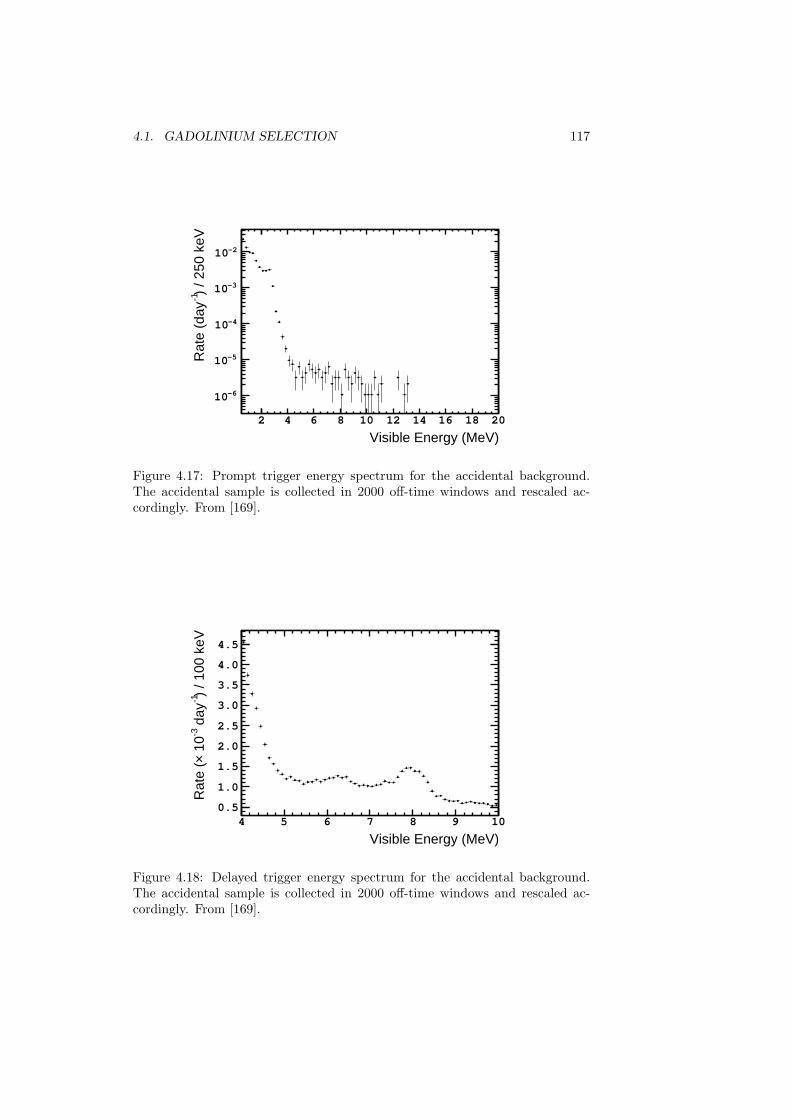
4.1. GADOLINIUM SELECTION 117
Visible Energy (MeV)2 4 6 8 10 12 14 16 18 20
) / 2
50 k
eV-1
Rat
e (d
ay
-610
-510
-410
-310
-210
Figure 4.17: Prompt trigger energy spectrum for the accidental background.The accidental sample is collected in 2000 off-time windows and rescaled ac-cordingly. From [169].
Visible Energy (MeV)4 5 6 7 8 9 10
) / 1
00 k
eV-1
day
-3 1
0×
Rat
e (
0.5
1.0
1.5
2.0
2.5
3.0
3.5
4.0
4.5
Figure 4.18: Delayed trigger energy spectrum for the accidental background.The accidental sample is collected in 2000 off-time windows and rescaled ac-cordingly. From [169].
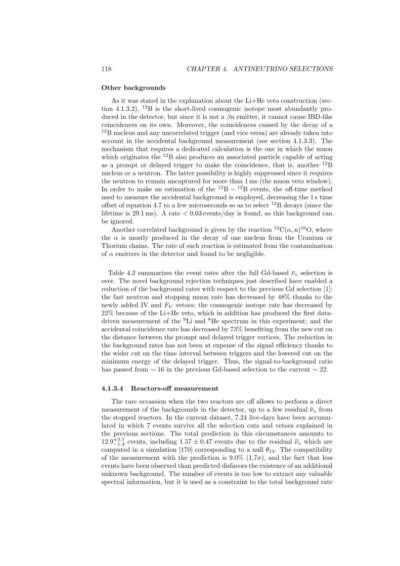
118 CHAPTER 4. ANTINEUTRINO SELECTIONS
Other backgrounds
As it was stated in the explanation about the Li+He veto construction (sec-tion 4.1.3.2), 12B is the short-lived cosmogenic isotope most abundantly pro-duced in the detector, but since it is not a βn emitter, it cannot cause IBD-likecoincidences on its own. Moreover, the coincidences caused by the decay of a12B nucleus and any uncorrelated trigger (and vice versa) are already taken intoaccount in the accidental background measurement (see section 4.1.3.3). Themechanism that requires a dedicated calculation is the one in which the muonwhich originates the 12B also produces an associated particle capable of actingas a prompt or delayed trigger to make the coincidence, that is, another 12Bnucleus or a neutron. The latter possibility is highly suppressed since it requiresthe neutron to remain uncaptured for more than 1 ms (the muon veto window).In order to make an estimation of the 12B − 12B events, the off-time methodused to measure the accidental background is employed, decreasing the 1 s timeoffset of equation 4.7 to a few microseconds so as to select 12B decays (since thelifetime is 29.1 ms). A rate < 0.03 events/day is found, so this background canbe ignored.
Another correlated background is given by the reaction 13C(α,n)16O, wherethe α is mostly produced in the decay of one nucleus from the Uranium orThorium chains. The rate of such reaction is estimated from the contaminationof α emitters in the detector and found to be negligible.
Table 4.2 summarizes the event rates after the full Gd-based νe selection isover. The novel background rejection techniques just described have enabled areduction of the background rates with respect to the previous Gd selection [1]:the fast neutron and stopping muon rate has decreased by 48% thanks to thenewly added IV and FV vetoes; the cosmogenic isotope rate has decreased by22% because of the Li+He veto, which in addition has produced the first data-driven measurement of the 9Li and 8He spectrum in this experiment; and theaccidental coincidence rate has decreased by 73% benefiting from the new cut onthe distance between the prompt and delayed trigger vertices. The reduction inthe background rates has not been at expense of the signal efficiency thanks tothe wider cut on the time interval between triggers and the lowered cut on theminimum energy of the delayed trigger. Thus, the signal-to-background ratiohas passed from ∼ 16 in the previous Gd-based selection to the current ∼ 22.
4.1.3.4 Reactors-off measurement
The rare occassion when the two reactors are off allows to perform a directmeasurement of the backgrounds in the detector, up to a few residual νe fromthe stopped reactors. In the current dataset, 7.24 live-days have been accumu-lated in which 7 events survive all the selection cuts and vetoes explained inthe previous sections. The total prediction in this circumstances amounts to12.9+3.1
−1.4 events, including 1.57 ± 0.47 events due to the residual νe which arecomputed in a simulation [170] corresponding to a null θ13. The compatibilityof the measurement with the prediction is 9.0% (1.7σ), and the fact that lessevents have been observed than predicted disfavors the existence of an additionalunknown background. The number of events is too low to extract any valuablespectral information, but it is used as a constraint to the total background rate
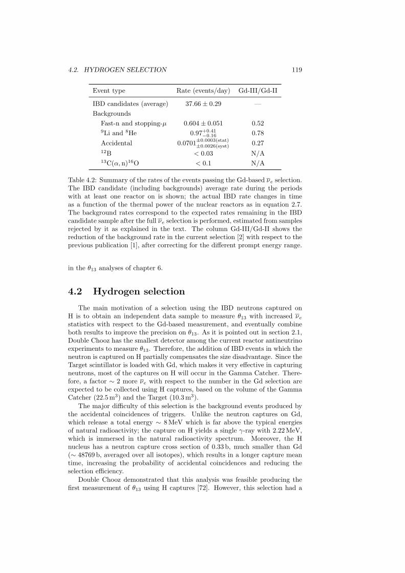
4.2. HYDROGEN SELECTION 119
Event type Rate (events/day) Gd-III/Gd-II
IBD candidates (average) 37.66± 0.29 —Backgrounds
Fast-n and stopping-µ 0.604± 0.051 0.529Li and 8He 0.97+0.41
−0.16 0.78Accidental 0.0701±0.0003(stat)
±0.0026(syst) 0.2712B < 0.03 N/A13C(α,n)16O < 0.1 N/A
Table 4.2: Summary of the rates of the events passing the Gd-based νe selection.The IBD candidate (including backgrounds) average rate during the periodswith at least one reactor on is shown; the actual IBD rate changes in timeas a function of the thermal power of the nuclear reactors as in equation 2.7.The background rates correspond to the expected rates remaining in the IBDcandidate sample after the full νe selection is performed, estimated from samplesrejected by it as explained in the text. The column Gd-III/Gd-II shows thereduction of the background rate in the current selection [2] with respect to theprevious publication [1], after correcting for the different prompt energy range.
in the θ13 analyses of chapter 6.
4.2 Hydrogen selection
The main motivation of a selection using the IBD neutrons captured onH is to obtain an independent data sample to measure θ13 with increased νestatistics with respect to the Gd-based measurement, and eventually combineboth results to improve the precision on θ13. As it is pointed out in section 2.1,Double Chooz has the smallest detector among the current reactor antineutrinoexperiments to measure θ13. Therefore, the addition of IBD events in which theneutron is captured on H partially compensates the size disadvantage. Since theTarget scintillator is loaded with Gd, which makes it very effective in capturingneutrons, most of the captures on H will occur in the Gamma Catcher. There-fore, a factor ∼ 2 more νe with respect to the number in the Gd selection areexpected to be collected using H captures, based on the volume of the GammaCatcher (22.5 m3) and the Target (10.3 m3).
The major difficulty of this selection is the background events produced bythe accidental coincidences of triggers. Unlike the neutron captures on Gd,which release a total energy ∼ 8 MeV which is far above the typical energiesof natural radioactivity; the capture on H yields a single γ-ray with 2.22 MeV,which is immersed in the natural radioactivity spectrum. Moreover, the Hnucleus has a neutron capture cross section of 0.33 b, much smaller than Gd(∼ 48769 b, averaged over all isotopes), which results in a longer capture meantime, increasing the probability of accidental coincidences and reducing theselection efficiency.
Double Chooz demonstrated that this analysis was feasible producing thefirst measurement of θ13 using H captures [72]. However, this selection had a
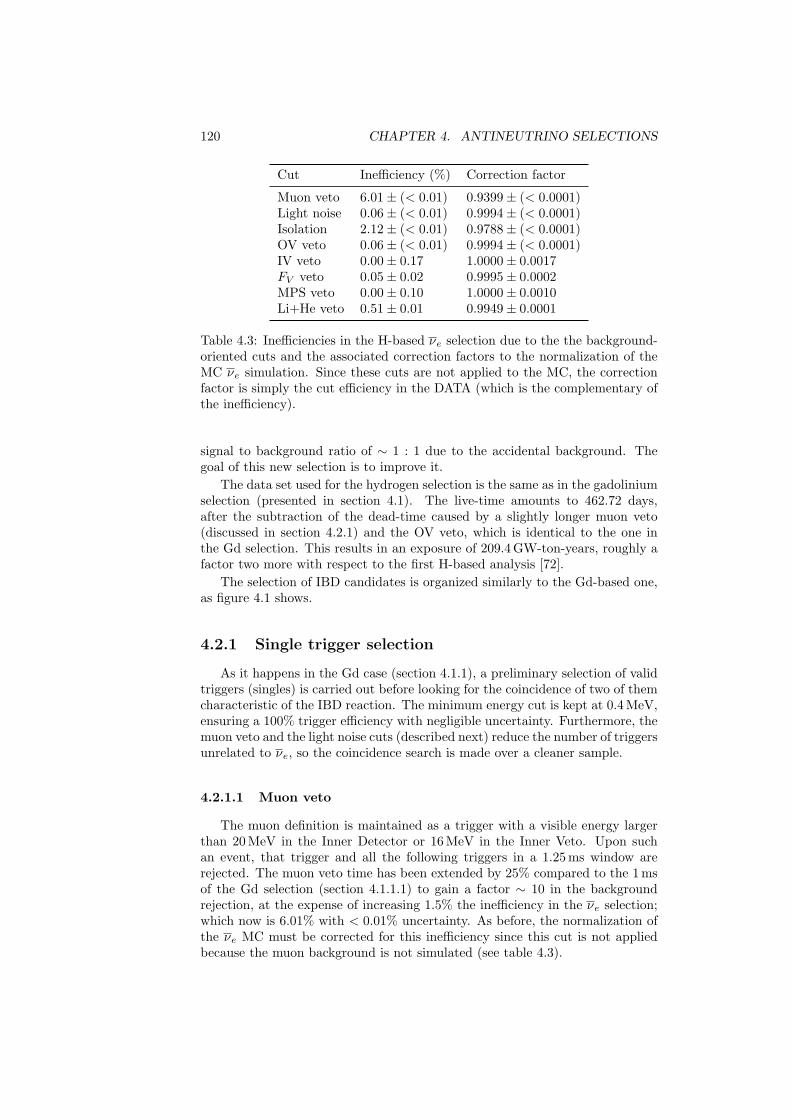
120 CHAPTER 4. ANTINEUTRINO SELECTIONS
Cut Inefficiency (%) Correction factor
Muon veto 6.01± (< 0.01) 0.9399± (< 0.0001)Light noise 0.06± (< 0.01) 0.9994± (< 0.0001)Isolation 2.12± (< 0.01) 0.9788± (< 0.0001)OV veto 0.06± (< 0.01) 0.9994± (< 0.0001)IV veto 0.00± 0.17 1.0000± 0.0017FV veto 0.05± 0.02 0.9995± 0.0002MPS veto 0.00± 0.10 1.0000± 0.0010Li+He veto 0.51± 0.01 0.9949± 0.0001
Table 4.3: Inefficiencies in the H-based νe selection due to the the background-oriented cuts and the associated correction factors to the normalization of theMC νe simulation. Since these cuts are not applied to the MC, the correctionfactor is simply the cut efficiency in the DATA (which is the complementary ofthe inefficiency).
signal to background ratio of ∼ 1 : 1 due to the accidental background. Thegoal of this new selection is to improve it.
The data set used for the hydrogen selection is the same as in the gadoliniumselection (presented in section 4.1). The live-time amounts to 462.72 days,after the subtraction of the dead-time caused by a slightly longer muon veto(discussed in section 4.2.1) and the OV veto, which is identical to the one inthe Gd selection. This results in an exposure of 209.4 GW-ton-years, roughly afactor two more with respect to the first H-based analysis [72].
The selection of IBD candidates is organized similarly to the Gd-based one,as figure 4.1 shows.
4.2.1 Single trigger selection
As it happens in the Gd case (section 4.1.1), a preliminary selection of validtriggers (singles) is carried out before looking for the coincidence of two of themcharacteristic of the IBD reaction. The minimum energy cut is kept at 0.4 MeV,ensuring a 100% trigger efficiency with negligible uncertainty. Furthermore, themuon veto and the light noise cuts (described next) reduce the number of triggersunrelated to νe, so the coincidence search is made over a cleaner sample.
4.2.1.1 Muon veto
The muon definition is maintained as a trigger with a visible energy largerthan 20 MeV in the Inner Detector or 16 MeV in the Inner Veto. Upon suchan event, that trigger and all the following triggers in a 1.25 ms window arerejected. The muon veto time has been extended by 25% compared to the 1 msof the Gd selection (section 4.1.1.1) to gain a factor ∼ 10 in the backgroundrejection, at the expense of increasing 1.5% the inefficiency in the νe selection;which now is 6.01% with < 0.01% uncertainty. As before, the normalization ofthe νe MC must be corrected for this inefficiency since this cut is not appliedbecause the muon background is not simulated (see table 4.3).
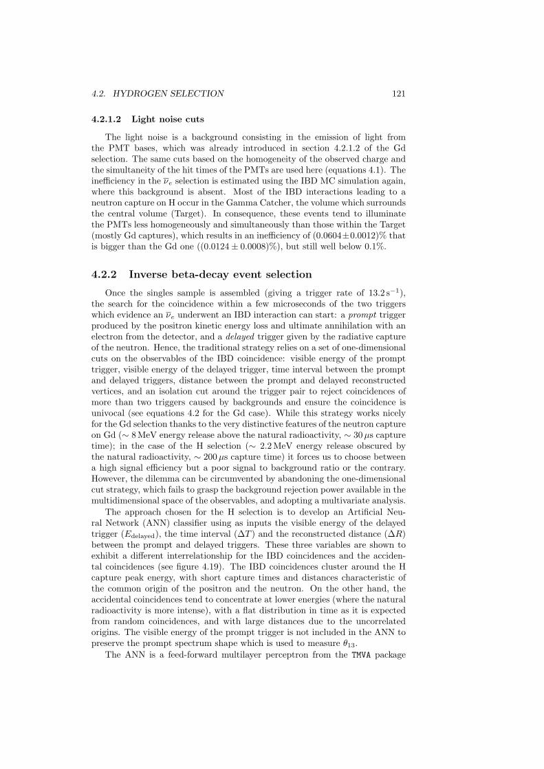
4.2. HYDROGEN SELECTION 121
4.2.1.2 Light noise cuts
The light noise is a background consisting in the emission of light fromthe PMT bases, which was already introduced in section 4.2.1.2 of the Gdselection. The same cuts based on the homogeneity of the observed charge andthe simultaneity of the hit times of the PMTs are used here (equations 4.1). Theinefficiency in the νe selection is estimated using the IBD MC simulation again,where this background is absent. Most of the IBD interactions leading to aneutron capture on H occur in the Gamma Catcher, the volume which surroundsthe central volume (Target). In consequence, these events tend to illuminatethe PMTs less homogeneously and simultaneously than those within the Target(mostly Gd captures), which results in an inefficiency of (0.0604±0.0012)% thatis bigger than the Gd one ((0.0124± 0.0008)%), but still well below 0.1%.
4.2.2 Inverse beta-decay event selection
Once the singles sample is assembled (giving a trigger rate of 13.2 s−1),the search for the coincidence within a few microseconds of the two triggerswhich evidence an νe underwent an IBD interaction can start: a prompt triggerproduced by the positron kinetic energy loss and ultimate annihilation with anelectron from the detector, and a delayed trigger given by the radiative captureof the neutron. Hence, the traditional strategy relies on a set of one-dimensionalcuts on the observables of the IBD coincidence: visible energy of the prompttrigger, visible energy of the delayed trigger, time interval between the promptand delayed triggers, distance between the prompt and delayed reconstructedvertices, and an isolation cut around the trigger pair to reject coincidences ofmore than two triggers caused by backgrounds and ensure the coincidence isunivocal (see equations 4.2 for the Gd case). While this strategy works nicelyfor the Gd selection thanks to the very distinctive features of the neutron captureon Gd (∼ 8 MeV energy release above the natural radioactivity, ∼ 30µs capturetime); in the case of the H selection (∼ 2.2 MeV energy release obscured bythe natural radioactivity, ∼ 200µs capture time) it forces us to choose betweena high signal efficiency but a poor signal to background ratio or the contrary.However, the dilemma can be circumvented by abandoning the one-dimensionalcut strategy, which fails to grasp the background rejection power available in themultidimensional space of the observables, and adopting a multivariate analysis.
The approach chosen for the H selection is to develop an Artificial Neu-ral Network (ANN) classifier using as inputs the visible energy of the delayedtrigger (Edelayed), the time interval (∆T ) and the reconstructed distance (∆R)between the prompt and delayed triggers. These three variables are shown toexhibit a different interrelationship for the IBD coincidences and the acciden-tal coincidences (see figure 4.19). The IBD coincidences cluster around the Hcapture peak energy, with short capture times and distances characteristic ofthe common origin of the positron and the neutron. On the other hand, theaccidental coincidences tend to concentrate at lower energies (where the naturalradioactivity is more intense), with a flat distribution in time as it is expectedfrom random coincidences, and with large distances due to the uncorrelatedorigins. The visible energy of the prompt trigger is not included in the ANN topreserve the prompt spectrum shape which is used to measure θ13.
The ANN is a feed-forward multilayer perceptron from the TMVA package
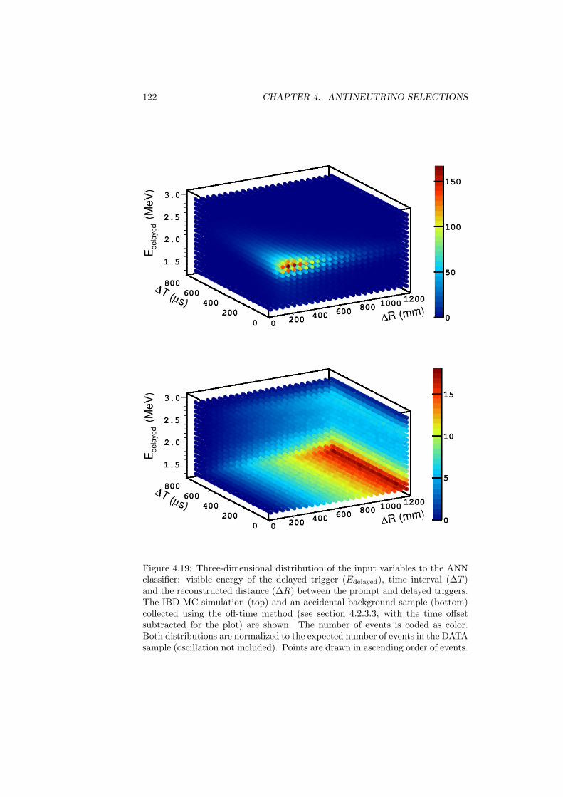
122 CHAPTER 4. ANTINEUTRINO SELECTIONS
Figure 4.19: Three-dimensional distribution of the input variables to the ANNclassifier: visible energy of the delayed trigger (Edelayed), time interval (∆T )and the reconstructed distance (∆R) between the prompt and delayed triggers.The IBD MC simulation (top) and an accidental background sample (bottom)collected using the off-time method (see section 4.2.3.3; with the time offsetsubtracted for the plot) are shown. The number of events is coded as color.Both distributions are normalized to the expected number of events in the DATAsample (oscillation not included). Points are drawn in ascending order of events.
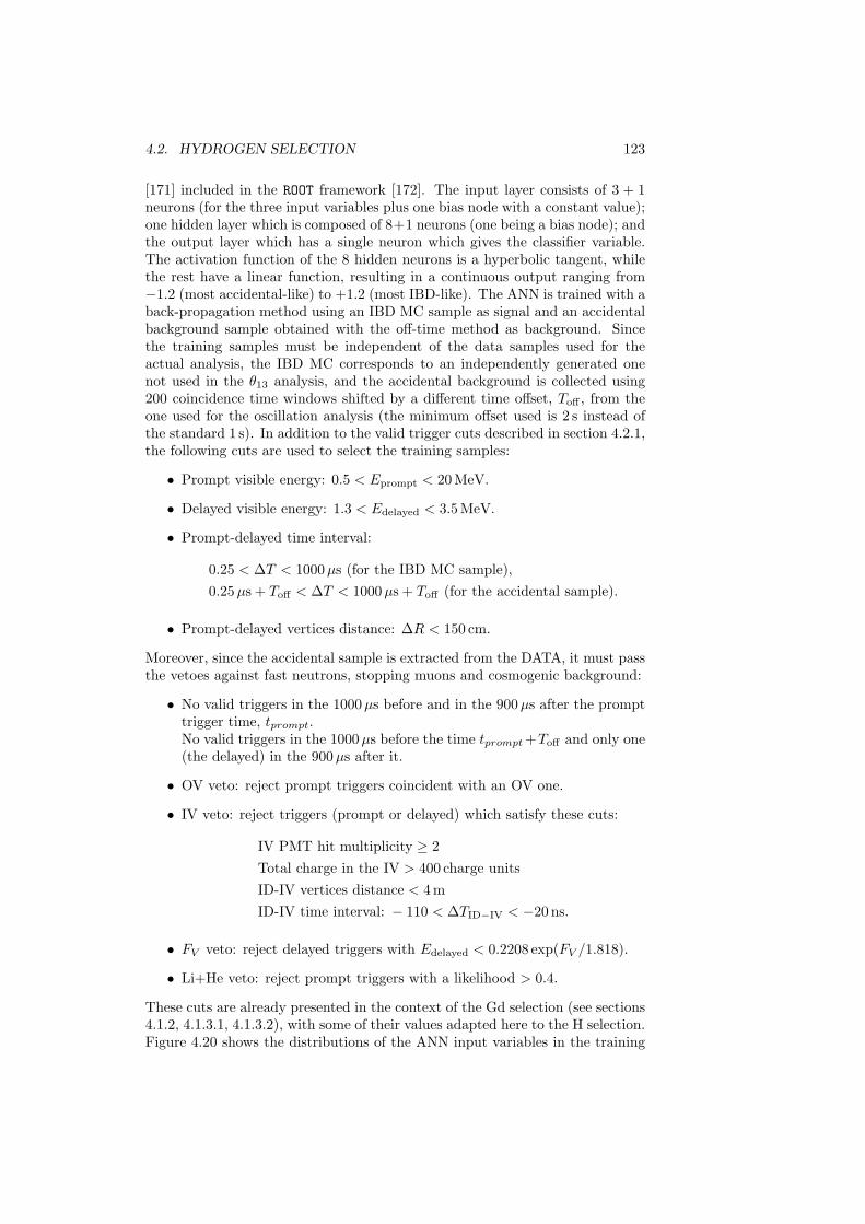
4.2. HYDROGEN SELECTION 123
[171] included in the ROOT framework [172]. The input layer consists of 3 + 1neurons (for the three input variables plus one bias node with a constant value);one hidden layer which is composed of 8+1 neurons (one being a bias node); andthe output layer which has a single neuron which gives the classifier variable.The activation function of the 8 hidden neurons is a hyperbolic tangent, whilethe rest have a linear function, resulting in a continuous output ranging from−1.2 (most accidental-like) to +1.2 (most IBD-like). The ANN is trained with aback-propagation method using an IBD MC sample as signal and an accidentalbackground sample obtained with the off-time method as background. Sincethe training samples must be independent of the data samples used for theactual analysis, the IBD MC corresponds to an independently generated onenot used in the θ13 analysis, and the accidental background is collected using200 coincidence time windows shifted by a different time offset, Toff , from theone used for the oscillation analysis (the minimum offset used is 2 s instead ofthe standard 1 s). In addition to the valid trigger cuts described in section 4.2.1,the following cuts are used to select the training samples:
• Prompt visible energy: 0.5 < Eprompt < 20 MeV.
• Delayed visible energy: 1.3 < Edelayed < 3.5 MeV.
• Prompt-delayed time interval:
0.25 < ∆T < 1000µs (for the IBD MC sample),0.25µs + Toff < ∆T < 1000µs + Toff (for the accidental sample).
• Prompt-delayed vertices distance: ∆R < 150 cm.
Moreover, since the accidental sample is extracted from the DATA, it must passthe vetoes against fast neutrons, stopping muons and cosmogenic background:
• No valid triggers in the 1000µs before and in the 900µs after the prompttrigger time, tprompt.No valid triggers in the 1000µs before the time tprompt+Toff and only one(the delayed) in the 900µs after it.
• OV veto: reject prompt triggers coincident with an OV one.
• IV veto: reject triggers (prompt or delayed) which satisfy these cuts:
IV PMT hit multiplicity ≥ 2Total charge in the IV > 400 charge unitsID-IV vertices distance < 4 mID-IV time interval: − 110 < ∆TID−IV < −20 ns.
• FV veto: reject delayed triggers with Edelayed < 0.2208 exp(FV /1.818).
• Li+He veto: reject prompt triggers with a likelihood > 0.4.
These cuts are already presented in the context of the Gd selection (see sections4.1.2, 4.1.3.1, 4.1.3.2), with some of their values adapted here to the H selection.Figure 4.20 shows the distributions of the ANN input variables in the training
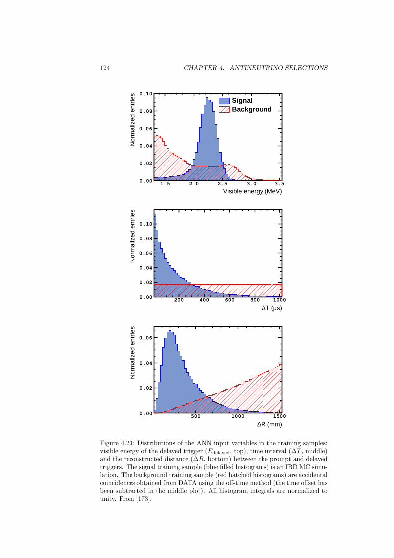
124 CHAPTER 4. ANTINEUTRINO SELECTIONS
Visible energy (MeV)1.5 2.0 2.5 3.0 3.5
Nor
mal
ized
ent
ries
0.00
0.02
0.04
0.06
0.08
0.10
SignalBackground
s)µT (∆200 400 600 800 1000
Nor
mal
ized
ent
ries
0.00
0.02
0.04
0.06
0.08
0.10
R (mm)∆500 1000 1500
Nor
mal
ized
ent
ries
0.00
0.02
0.04
0.06
Figure 4.20: Distributions of the ANN input variables in the training samples:visible energy of the delayed trigger (Edelayed, top), time interval (∆T , middle)and the reconstructed distance (∆R, bottom) between the prompt and delayedtriggers. The signal training sample (blue filled histograms) is an IBD MC simu-lation. The background training sample (red hatched histograms) are accidentalcoincidences obtained from DATA using the off-time method (the time offset hasbeen subtracted in the middle plot). All histogram integrals are normalized tounity. From [173].
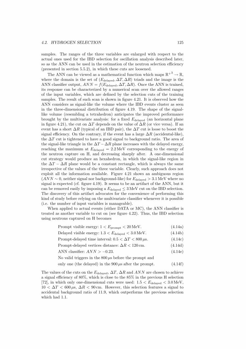
4.2. HYDROGEN SELECTION 125
samples. The ranges of the three variables are enlarged with respect to theactual ones used for the IBD selection for oscillation analysis described later,so as the ANN can be used in the estimation of the neutron selection efficiency(presented in section 5.5.2), in which these cuts are loosened.
The ANN can be viewed as a mathematical function which maps R+3 → R,where the domain is the set of (Edelayed,∆T,∆R) triads and the image is theANN classifier output, ANN = f(Edelayed,∆T,∆R). Once the ANN is trained,its response can be characterized by a numerical scan over the allowed rangesof the input variables, which are defined by the selection cuts of the trainingsamples. The result of such scan is shown in figure 4.21. It is observed how theANN considers as signal-like the volume where the IBD events cluster as seenin the three-dimensional distribution of figure 4.19. The shape of the signal-like volume (resembling a tetrahedron) anticipates the improved performancebrought by the multivariate analysis: for a fixed Edelayed (an horizontal planein figure 4.21), the cut on ∆T depends on the value of ∆R (or vice versa). If anevent has a short ∆R (typical of an IBD pair), the ∆T cut is loose to boost thesignal efficiency. On the contrary, if the event has a large ∆R (accidental-like),the ∆T cut is tightened to have a good signal to background ratio. The area ofthe signal-like triangle in the ∆T −∆R plane increases with the delayed energy,reaching the maximum at Edelayed = 2.2 MeV corresponding to the energy ofthe neutron capture on H, and decreasing sharply after. A one-dimensionalcut strategy would produce an hexahedron, in which the signal-like region inthe ∆T − ∆R plane would be a constant rectangle, which is always the sameirrespective of the values of the three variable. Clearly, such approach does notexploit all the information available. Figure 4.21 shows an ambiguous region(ANN ∼ 0, neither signal nor background-like) for Edelayed > 3.1 MeV where nosignal is expected (cf. figure 4.19). It seems to be an artifact of the ANN, but itcan be removed easily by imposing a Edelayed ≤ 3 MeV cut on the IBD selection.The discovery of this artifact advocates for the convenience of performing thiskind of study before relying on the multivariate classifier whenever it is possible(i.e. the number of input variables is manageable).
When applied to actual events (either DATA or MC), the ANN classifier istreated as another variable to cut on (see figure 4.22). Thus, the IBD selectionusing neutrons captured on H becomes
Prompt visible energy: 1 < Eprompt < 20 MeV. (4.14a)Delayed visible energy: 1.3 < Edelayed < 3.0 MeV. (4.14b)Prompt-delayed time interval: 0.5 < ∆T < 800µs. (4.14c)Prompt-delayed vertices distance: ∆R < 120 cm. (4.14d)ANN classifier: ANN > −0.23. (4.14e)No valid triggers in the 800µs before the prompt andonly one (the delayed) in the 900µs after the prompt. (4.14f)
The values of the cuts on the Edelayed, ∆T , ∆R and ANN are chosen to achievea signal efficiency of 80%, which is close to the 85% in the previous H selection[72], in which only one-dimensional cuts were used: 1.5 < Edelayed < 3.0 MeV,10 < ∆T < 600µs, ∆R < 90 cm. However, this selection features a signal toaccidental background ratio of 11.9, which outperforms the previous selectionwhich had 1.1.
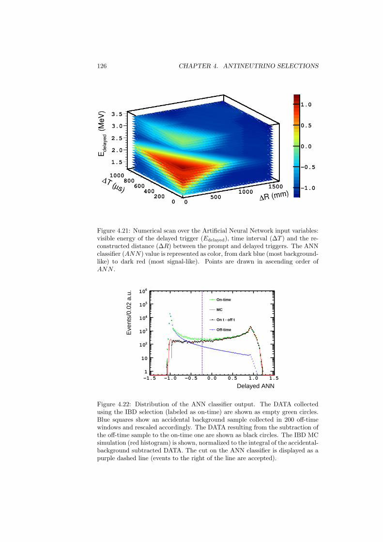
126 CHAPTER 4. ANTINEUTRINO SELECTIONS
Figure 4.21: Numerical scan over the Artificial Neural Network input variables:visible energy of the delayed trigger (Edelayed), time interval (∆T ) and the re-constructed distance (∆R) between the prompt and delayed triggers. The ANNclassifier (ANN) value is represented as color, from dark blue (most background-like) to dark red (most signal-like). Points are drawn in ascending order ofANN .
Delayed ANN-1.5 -1.0 -0.5 0.0 0.5 1.0 1.5
Eve
nts/
0.02
a.u
.
1
10
210
310
410
510
610
On-time
MC
On t - off t
Off-time
Figure 4.22: Distribution of the ANN classifier output. The DATA collectedusing the IBD selection (labeled as on-time) are shown as empty green circles.Blue squares show an accidental background sample collected in 200 off-timewindows and rescaled accordingly. The DATA resulting from the subtraction ofthe off-time sample to the on-time one are shown as black circles. The IBD MCsimulation (red histogram) is shown, normalized to the integral of the accidental-background subtracted DATA. The cut on the ANN classifier is displayed as apurple dashed line (events to the right of the line are accepted).
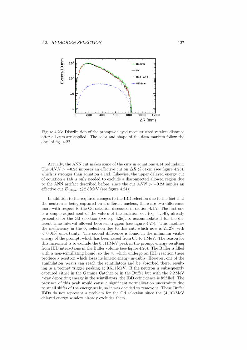
4.2. HYDROGEN SELECTION 127
R (mm)∆ 0 200 400 600 800 1000 1200
Eve
nts/
10 m
m
1
10
210
310 On-time
MC
On t - off t
Off-time
Figure 4.23: Distribution of the prompt-delayed reconstructed vertices distanceafter all cuts are applied. The color and shape of the data markers follow theones of fig. 4.22.
Actually, the ANN cut makes some of the cuts in equations 4.14 redundant.The ANN > −0.23 imposes an effective cut on ∆R . 84 cm (see figure 4.23),which is stronger than equation 4.14d. Likewise, the upper delayed energy cutof equation 4.14b is only needed to exclude a disconnected allowed region dueto the ANN artifact described before, since the cut ANN > −0.23 implies aneffective cut Edelayed . 2.8 MeV (see figure 4.24).
In addition to the required changes to the IBD selection due to the fact thatthe neutron is being captured on a different nucleus, there are two differencesmore with respect to the Gd selection discussed in section 4.1.2. The first oneis a simple adjustment of the values of the isolation cut (eq. 4.14f), alreadypresented for the Gd selection (see eq. 4.2e), to accommodate it for the dif-ferent time interval allowed between triggers (see figure 4.25). This modifiesthe inefficiency in the νe selection due to this cut, which now is 2.12% with< 0.01% uncertainty. The second difference is found in the minimum visibleenergy of the prompt, which has been raised from 0.5 to 1 MeV. The reason forthis increment is to exclude the 0.511 MeV peak in the prompt energy resultingfrom IBD interactions in the Buffer volume (see figure 4.26). The Buffer is filledwith a non-scintillating liquid, so the νe which undergo an IBD reaction thereproduce a positron which loses its kinetic energy invisibly. However, one of theannihilation γ-rays can reach the scintillators and be absorbed there, result-ing in a prompt trigger peaking at 0.511 MeV. If the neutron is subsequentlycaptured either in the Gamma Catcher or in the Buffer but with the 2.2 MeVγ-ray depositing energy in the scintillators, the IBD coincidence is fulfilled. Thepresence of this peak would cause a significant normalization uncertainty dueto small shifts of the energy scale, so it was decided to remove it. These BufferIBDs do not represent a problem for the Gd selection since the (4, 10) MeVdelayed energy window already excludes them.
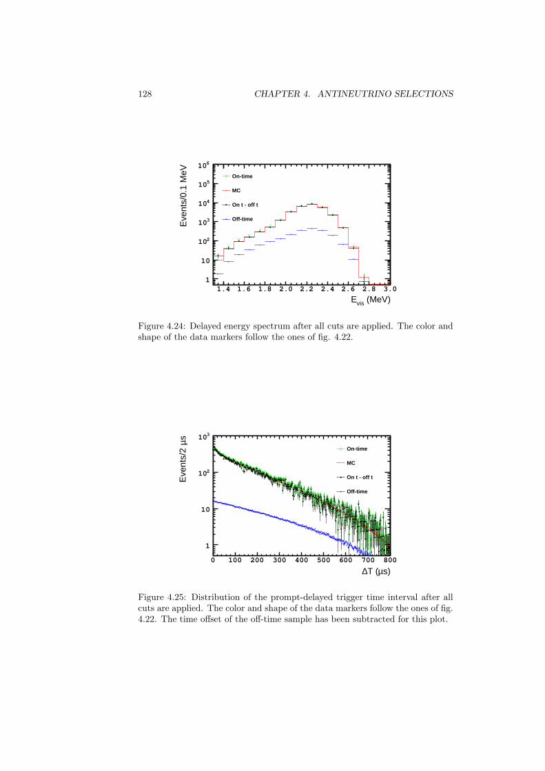
128 CHAPTER 4. ANTINEUTRINO SELECTIONS
(MeV)vis E1.4 1.6 1.8 2.0 2.2 2.4 2.6 2.8 3.0
Eve
nts/
0.1
MeV
1
10
210
310
410
510
610
On-time
MC
On t - off t
Off-time
Figure 4.24: Delayed energy spectrum after all cuts are applied. The color andshape of the data markers follow the ones of fig. 4.22.
s)µT (∆ 0 100 200 300 400 500 600 700 800
sµ E
vent
s/2
1
10
210
310
On-time
MC
On t - off t
Off-time
Figure 4.25: Distribution of the prompt-delayed trigger time interval after allcuts are applied. The color and shape of the data markers follow the ones of fig.4.22. The time offset of the off-time sample has been subtracted for this plot.
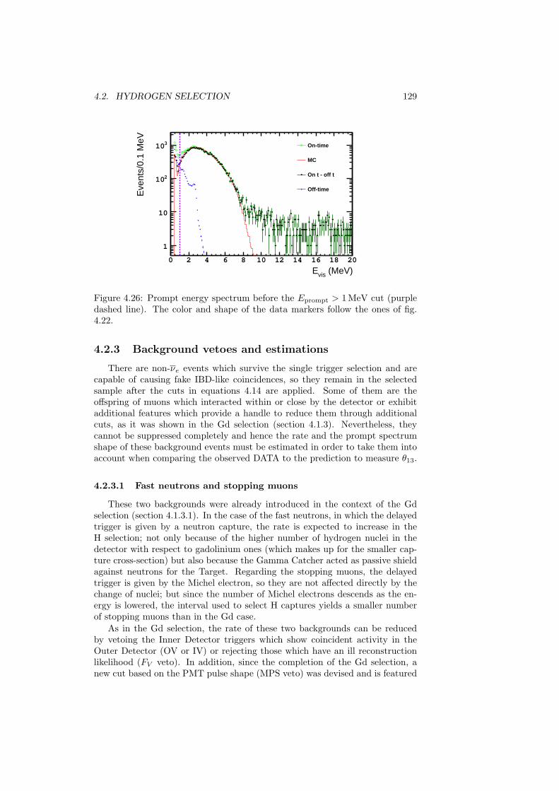
4.2. HYDROGEN SELECTION 129
(MeV)vis E0 2 4 6 8 10 12 14 16 18 20
Eve
nts/
0.1
MeV
1
10
210
310 On-time
MC
On t - off t
Off-time
Figure 4.26: Prompt energy spectrum before the Eprompt > 1 MeV cut (purpledashed line). The color and shape of the data markers follow the ones of fig.4.22.
4.2.3 Background vetoes and estimations
There are non-νe events which survive the single trigger selection and arecapable of causing fake IBD-like coincidences, so they remain in the selectedsample after the cuts in equations 4.14 are applied. Some of them are theoffspring of muons which interacted within or close by the detector or exhibitadditional features which provide a handle to reduce them through additionalcuts, as it was shown in the Gd selection (section 4.1.3). Nevertheless, theycannot be suppressed completely and hence the rate and the prompt spectrumshape of these background events must be estimated in order to take them intoaccount when comparing the observed DATA to the prediction to measure θ13.
4.2.3.1 Fast neutrons and stopping muons
These two backgrounds were already introduced in the context of the Gdselection (section 4.1.3.1). In the case of the fast neutrons, in which the delayedtrigger is given by a neutron capture, the rate is expected to increase in theH selection; not only because of the higher number of hydrogen nuclei in thedetector with respect to gadolinium ones (which makes up for the smaller cap-ture cross-section) but also because the Gamma Catcher acted as passive shieldagainst neutrons for the Target. Regarding the stopping muons, the delayedtrigger is given by the Michel electron, so they are not affected directly by thechange of nuclei; but since the number of Michel electrons descends as the en-ergy is lowered, the interval used to select H captures yields a smaller numberof stopping muons than in the Gd case.
As in the Gd selection, the rate of these two backgrounds can be reducedby vetoing the Inner Detector triggers which show coincident activity in theOuter Detector (OV or IV) or rejecting those which have an ill reconstructionlikelihood (FV veto). In addition, since the completion of the Gd selection, anew cut based on the PMT pulse shape (MPS veto) was devised and is featured
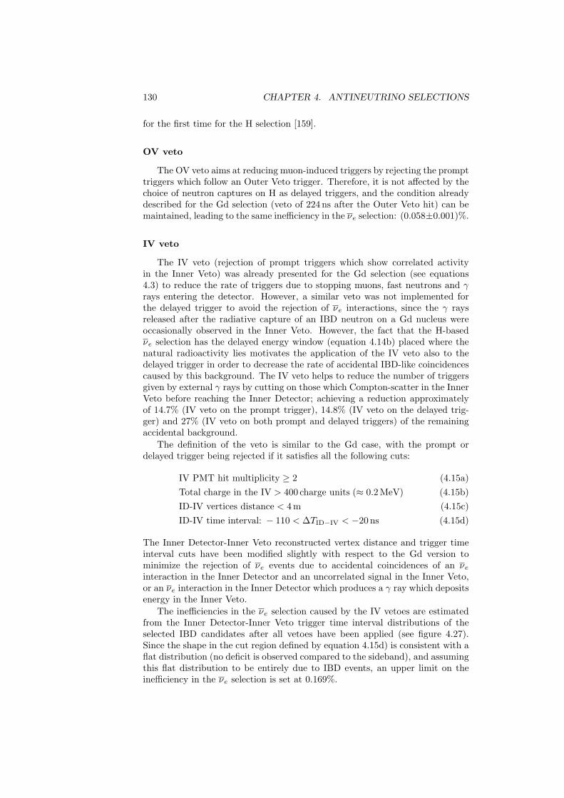
130 CHAPTER 4. ANTINEUTRINO SELECTIONS
for the first time for the H selection [159].
OV veto
The OV veto aims at reducing muon-induced triggers by rejecting the prompttriggers which follow an Outer Veto trigger. Therefore, it is not affected by thechoice of neutron captures on H as delayed triggers, and the condition alreadydescribed for the Gd selection (veto of 224 ns after the Outer Veto hit) can bemaintained, leading to the same inefficiency in the νe selection: (0.058±0.001)%.
IV veto
The IV veto (rejection of prompt triggers which show correlated activityin the Inner Veto) was already presented for the Gd selection (see equations4.3) to reduce the rate of triggers due to stopping muons, fast neutrons and γrays entering the detector. However, a similar veto was not implemented forthe delayed trigger to avoid the rejection of νe interactions, since the γ raysreleased after the radiative capture of an IBD neutron on a Gd nucleus wereoccasionally observed in the Inner Veto. However, the fact that the H-basedνe selection has the delayed energy window (equation 4.14b) placed where thenatural radioactivity lies motivates the application of the IV veto also to thedelayed trigger in order to decrease the rate of accidental IBD-like coincidencescaused by this background. The IV veto helps to reduce the number of triggersgiven by external γ rays by cutting on those which Compton-scatter in the InnerVeto before reaching the Inner Detector; achieving a reduction approximatelyof 14.7% (IV veto on the prompt trigger), 14.8% (IV veto on the delayed trig-ger) and 27% (IV veto on both prompt and delayed triggers) of the remainingaccidental background.
The definition of the veto is similar to the Gd case, with the prompt ordelayed trigger being rejected if it satisfies all the following cuts:
IV PMT hit multiplicity ≥ 2 (4.15a)Total charge in the IV > 400 charge units (≈ 0.2 MeV) (4.15b)ID-IV vertices distance < 4 m (4.15c)ID-IV time interval: − 110 < ∆TID−IV < −20 ns (4.15d)
The Inner Detector-Inner Veto reconstructed vertex distance and trigger timeinterval cuts have been modified slightly with respect to the Gd version tominimize the rejection of νe events due to accidental coincidences of an νeinteraction in the Inner Detector and an uncorrelated signal in the Inner Veto,or an νe interaction in the Inner Detector which produces a γ ray which depositsenergy in the Inner Veto.
The inefficiencies in the νe selection caused by the IV vetoes are estimatedfrom the Inner Detector-Inner Veto trigger time interval distributions of theselected IBD candidates after all vetoes have been applied (see figure 4.27).Since the shape in the cut region defined by equation 4.15d) is consistent with aflat distribution (no deficit is observed compared to the sideband), and assumingthis flat distribution to be entirely due to IBD events, an upper limit on theinefficiency in the νe selection is set at 0.169%.
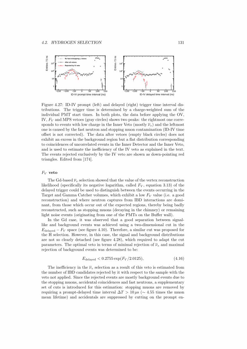
4.2. HYDROGEN SELECTION 131
ID-IV prompt time interval (ns)-150 -100 -50 0 50 100 150
Ent
ries
/ 5 n
s
1
10
210
310
vetoesµNo fast-n/stopping-
After all vetoes
Rejected by IV veto
ID-IV delayed time interval (ns)-150 -100 -50 0 50 100 150
Ent
ries
/ 5 n
s
1
10
210
310
Figure 4.27: ID-IV prompt (left) and delayed (right) trigger time interval dis-tributions. The trigger time is determined by a charge-weighted sum of theindividual PMT start times. In both plots, the data before applying the OV,IV, FV and MPS vetoes (gray circles) shows two peaks: the rightmost one corre-sponds to events with low charge in the Inner Veto (mostly νe) and the leftmostone is caused by the fast neutron and stopping muon contamination (ID-IV timeoffset is not corrected). The data after vetoes (empty black circles) does notexhibit an excess in the background region but a flat distribution correspondingto coincidences of uncorrelated events in the Inner Detector and the Inner Veto,and is used to estimate the inefficiency of the IV veto as explained in the text.The events rejected exclusively by the IV veto are shown as down-pointing redtriangles. Edited from [174].
FV veto
The Gd-based νe selection showed that the value of the vertex reconstructionlikelihood (specifically its negative logarithm, called FV , equation 3.13) of thedelayed trigger could be used to distinguish between the events occurring in theTarget and Gamma Catcher volumes, which exhibit a low FV value (i.e. a goodreconstruction) and where neutron captures from IBD interactions are domi-nant, from those which occur out of the expected regions, thereby being badlyreconstructed, such as stopping muons (decaying in the chimney) or remaininglight noise events (originating from one of the PMTs on the Buffer wall).
In the Gd case, it was observed that a good separation between signal-like and background events was achieved using a two-dimensional cut in theEdelayed − FV space (see figure 4.10). Therefore, a similar cut was proposed forthe H selection. However, in this case, the signal and background distributionsare not so clearly detached (see figure 4.28), which required to adapt the cutparameters. The optimal veto in terms of minimal rejection of νe and maximalrejection of background events was determined to be:
Edelayed < 0.2755 exp(FV /2.0125), (4.16)
The inefficiency in the νe selection as a result of this veto is estimated fromthe number of IBD candidates rejected by it with respect to the sample with theveto not applied. Since the rejected events are mostly background events due tothe stopping muons, accidental coincidences and fast neutrons, a supplementaryset of cuts is introduced for this estimation: stopping muons are removed byrequiring a prompt-delayed time interval ∆T > 10µs (∼ 4.55 times the muonmean lifetime) and accidentals are suppressed by cutting on the prompt en-
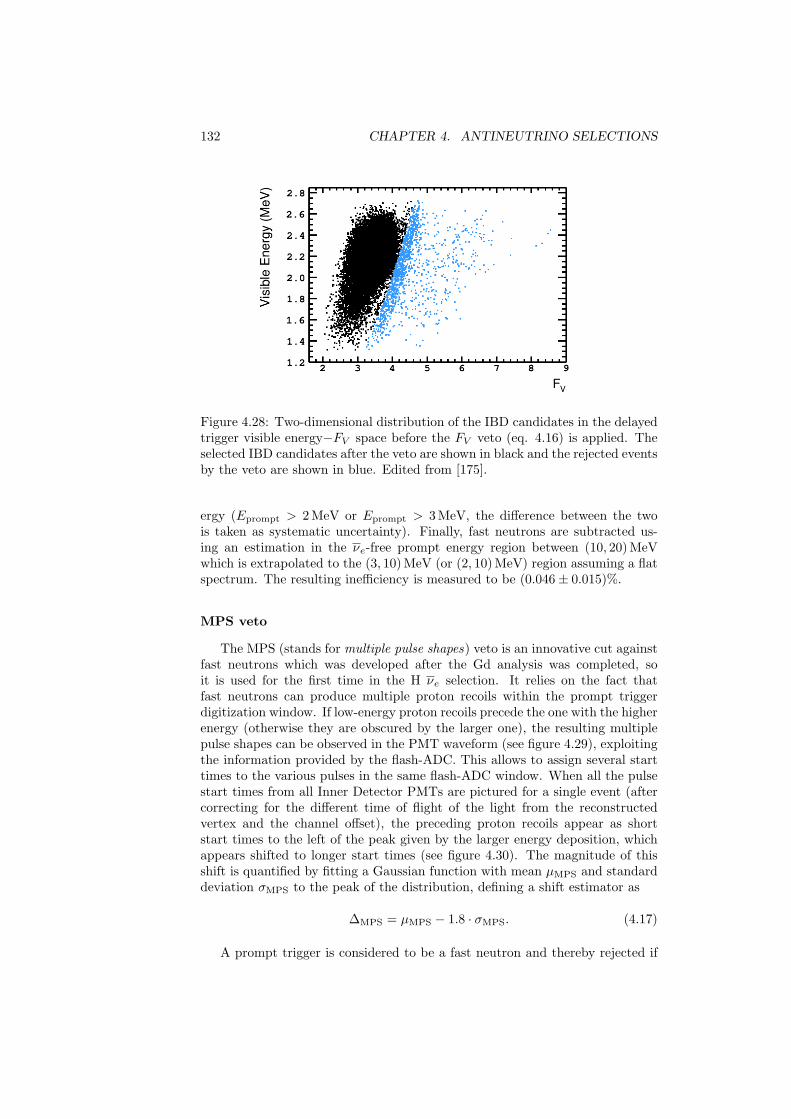
132 CHAPTER 4. ANTINEUTRINO SELECTIONS
Figure 4.28: Two-dimensional distribution of the IBD candidates in the delayedtrigger visible energy−FV space before the FV veto (eq. 4.16) is applied. Theselected IBD candidates after the veto are shown in black and the rejected eventsby the veto are shown in blue. Edited from [175].
ergy (Eprompt > 2 MeV or Eprompt > 3 MeV, the difference between the twois taken as systematic uncertainty). Finally, fast neutrons are subtracted us-ing an estimation in the νe-free prompt energy region between (10, 20) MeVwhich is extrapolated to the (3, 10) MeV (or (2, 10) MeV) region assuming a flatspectrum. The resulting inefficiency is measured to be (0.046± 0.015)%.
MPS veto
The MPS (stands for multiple pulse shapes) veto is an innovative cut againstfast neutrons which was developed after the Gd analysis was completed, soit is used for the first time in the H νe selection. It relies on the fact thatfast neutrons can produce multiple proton recoils within the prompt triggerdigitization window. If low-energy proton recoils precede the one with the higherenergy (otherwise they are obscured by the larger one), the resulting multiplepulse shapes can be observed in the PMT waveform (see figure 4.29), exploitingthe information provided by the flash-ADC. This allows to assign several starttimes to the various pulses in the same flash-ADC window. When all the pulsestart times from all Inner Detector PMTs are pictured for a single event (aftercorrecting for the different time of flight of the light from the reconstructedvertex and the channel offset), the preceding proton recoils appear as shortstart times to the left of the peak given by the larger energy deposition, whichappears shifted to longer start times (see figure 4.30). The magnitude of thisshift is quantified by fitting a Gaussian function with mean µMPS and standarddeviation σMPS to the peak of the distribution, defining a shift estimator as
∆MPS = µMPS − 1.8 · σMPS. (4.17)
A prompt trigger is considered to be a fast neutron and thereby rejected if
4.2. HYDROGEN SELECTION 133
time/2 (ns)0 20 40 60 80 100 120
FAD
C c
ou
nt
198
200
202
204
206
208
210
Figure 4.29: Example of one PMT waveform showing 2 pulses within the flash-ADC digitization window. The green horizontal line marks the reference base-line. The blue oblique lines show the results of linear fits to the leading edgesof the pulses. The interceptions of the oblique lines with the horizontal linedetermine the start times of the pulses (marked as red dots). From [176].
it satisfies
Eprompt ≥ 3 MeV and ∆MPS > 5 ns (4.18a)
or
1.2 MeV < Eprompt < 3 MeV and ∆MPS > 5 nsand is not tagged as ortho-positronium (4.18b)
The cut at 5 ns on ∆MPS was tuned to minimize the rejection of νe events.It was established analyzing the 60Co calibration data, which has negligiblefast-neutron contamination. The 60Co source, upon β− decay, releases twosequential γ-rays with energies 1.173 and 1.333 MeV [38] totaling ≈ 2.5 MeV,which is close to the mean prompt energy of the IBD events.
The energy dependence of the MPS veto is introduced to take into accountthe formation of ortho-positronium (o-Ps) by the positron emitted in the IBDreaction. o-Ps is the triplet state (3S1) of the positronium, and has a ∼ 45%formation fraction in the Double Chooz scintillators, with a mean lifetime of∼ 3.4 ns 5 [178]. o-Ps events also produce multiple pulse shapes, in which thefirst pulse is given by the positron ionization and the second pulse correspondsto the o-Ps decay into γ-rays totaling 1.022 MeV. In order to minimize theloss of IBD events, it is required that the o-Ps tagging algorithm (describedin reference [178]) does not identify the event as o-Ps. This algorithm triesto fit the distribution of pulse start times to two time profiles, the first one
5The mean lifetime of o-Ps in vacuum is 142 ns, but the interaction with the surroundingmedium accelerates the decay. There is another positronium state, the singlet (1S0) knownas para-positronium, but it is too short lived (O( ps)) to be relevant here.
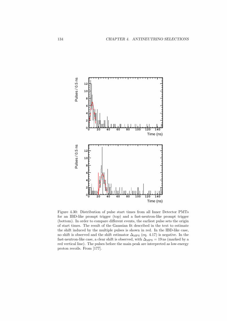
134 CHAPTER 4. ANTINEUTRINO SELECTIONS
Time (ns)0 20 40 60 80 100 120 140
Pul
ses
/ 0.5
ns
0
2
4
6
8
10
12
Time (ns)0 20 40 60 80 100 120 140
Pul
ses
/ 0.5
ns
0
2
4
6
8
10
12
Figure 4.30: Distribution of pulse start times from all Inner Detector PMTsfor an IBD-like prompt trigger (top) and a fast-neutron-like prompt trigger(bottom). In order to compare different events, the earliest pulse sets the originof start times. The result of the Gaussian fit described in the text to estimatethe shift induced by the multiple pulses is shown in red. In the IBD-like case,no shift is observed and the shift estimator ∆MPS (eq. 4.17) is negative. In thefast-neutron-like case, a clear shift is observed, with ∆MPS = 19 ns (marked by ared vertical line). The pulses before the main peak are interpreted as low-energyproton recoils. From [177].
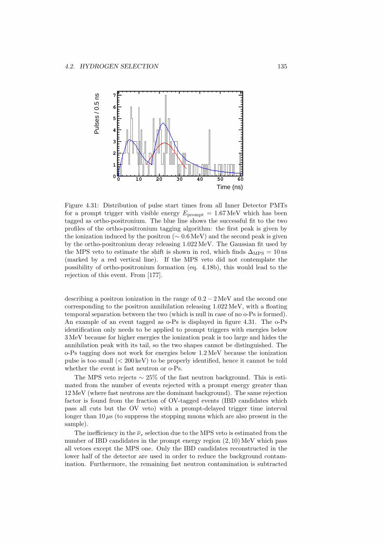
4.2. HYDROGEN SELECTION 135
Time (ns)0 10 20 30 40 50 60
Pul
ses
/ 0.5
ns
0
1
2
3
4
5
6
7
Figure 4.31: Distribution of pulse start times from all Inner Detector PMTsfor a prompt trigger with visible energy Eprompt = 1.67 MeV which has beentagged as ortho-positronium. The blue line shows the successful fit to the twoprofiles of the ortho-positronium tagging algorithm: the first peak is given bythe ionization induced by the positron (∼ 0.6 MeV) and the second peak is givenby the ortho-positronium decay releasing 1.022 MeV. The Gaussian fit used bythe MPS veto to estimate the shift is shown in red, which finds ∆MPS = 10 ns(marked by a red vertical line). If the MPS veto did not contemplate thepossibility of ortho-positronium formation (eq. 4.18b), this would lead to therejection of this event. From [177].
describing a positron ionization in the range of 0.2− 2 MeV and the second onecorresponding to the positron annihilation releasing 1.022 MeV, with a floatingtemporal separation between the two (which is null in case of no o-Ps is formed).An example of an event tagged as o-Ps is displayed in figure 4.31. The o-Psidentification only needs to be applied to prompt triggers with energies below3 MeV because for higher energies the ionization peak is too large and hides theannihilation peak with its tail, so the two shapes cannot be distinguished. Theo-Ps tagging does not work for energies below 1.2 MeV because the ionizationpulse is too small (< 200 keV) to be properly identified, hence it cannot be toldwhether the event is fast neutron or o-Ps.
The MPS veto rejects ∼ 25% of the fast neutron background. This is esti-mated from the number of events rejected with a prompt energy greater than12 MeV (where fast neutrons are the dominant background). The same rejectionfactor is found from the fraction of OV-tagged events (IBD candidates whichpass all cuts but the OV veto) with a prompt-delayed trigger time intervallonger than 10µs (to suppress the stopping muons which are also present in thesample).
The inefficiency in the νe selection due to the MPS veto is estimated from thenumber of IBD candidates in the prompt energy region (2, 10) MeV which passall vetoes except the MPS one. Only the IBD candidates reconstructed in thelower half of the detector are used in order to reduce the background contam-ination. Furthermore, the remaining fast neutron contamination is subtracted
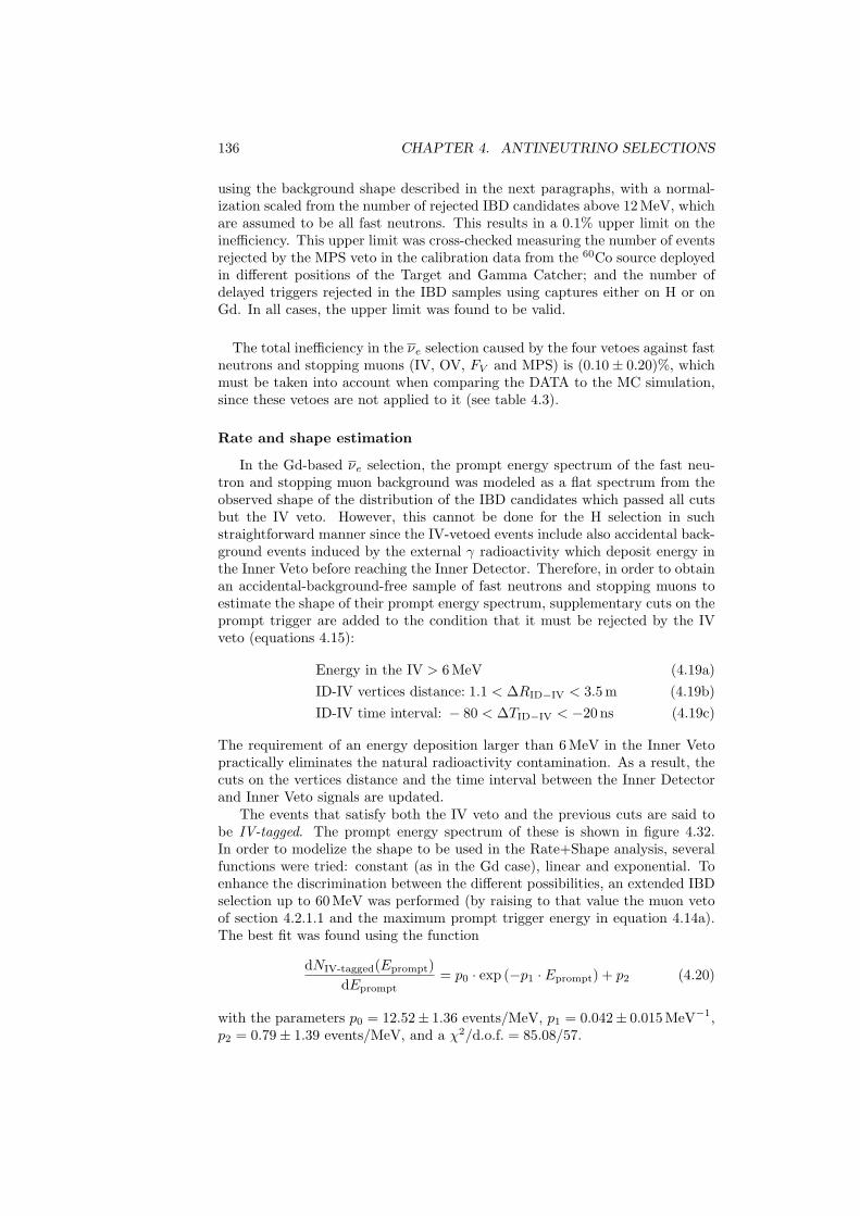
136 CHAPTER 4. ANTINEUTRINO SELECTIONS
using the background shape described in the next paragraphs, with a normal-ization scaled from the number of rejected IBD candidates above 12 MeV, whichare assumed to be all fast neutrons. This results in a 0.1% upper limit on theinefficiency. This upper limit was cross-checked measuring the number of eventsrejected by the MPS veto in the calibration data from the 60Co source deployedin different positions of the Target and Gamma Catcher; and the number ofdelayed triggers rejected in the IBD samples using captures either on H or onGd. In all cases, the upper limit was found to be valid.
The total inefficiency in the νe selection caused by the four vetoes against fastneutrons and stopping muons (IV, OV, FV and MPS) is (0.10± 0.20)%, whichmust be taken into account when comparing the DATA to the MC simulation,since these vetoes are not applied to it (see table 4.3).
Rate and shape estimation
In the Gd-based νe selection, the prompt energy spectrum of the fast neu-tron and stopping muon background was modeled as a flat spectrum from theobserved shape of the distribution of the IBD candidates which passed all cutsbut the IV veto. However, this cannot be done for the H selection in suchstraightforward manner since the IV-vetoed events include also accidental back-ground events induced by the external γ radioactivity which deposit energy inthe Inner Veto before reaching the Inner Detector. Therefore, in order to obtainan accidental-background-free sample of fast neutrons and stopping muons toestimate the shape of their prompt energy spectrum, supplementary cuts on theprompt trigger are added to the condition that it must be rejected by the IVveto (equations 4.15):
Energy in the IV > 6 MeV (4.19a)ID-IV vertices distance: 1.1 < ∆RID−IV < 3.5 m (4.19b)ID-IV time interval: − 80 < ∆TID−IV < −20 ns (4.19c)
The requirement of an energy deposition larger than 6 MeV in the Inner Vetopractically eliminates the natural radioactivity contamination. As a result, thecuts on the vertices distance and the time interval between the Inner Detectorand Inner Veto signals are updated.
The events that satisfy both the IV veto and the previous cuts are said tobe IV-tagged. The prompt energy spectrum of these is shown in figure 4.32.In order to modelize the shape to be used in the Rate+Shape analysis, severalfunctions were tried: constant (as in the Gd case), linear and exponential. Toenhance the discrimination between the different possibilities, an extended IBDselection up to 60 MeV was performed (by raising to that value the muon vetoof section 4.2.1.1 and the maximum prompt trigger energy in equation 4.14a).The best fit was found using the function
dNIV-tagged(Eprompt)dEprompt
= p0 · exp (−p1 · Eprompt) + p2 (4.20)
with the parameters p0 = 12.52± 1.36 events/MeV, p1 = 0.042± 0.015 MeV−1,p2 = 0.79± 1.39 events/MeV, and a χ2/d.o.f. = 85.08/57.
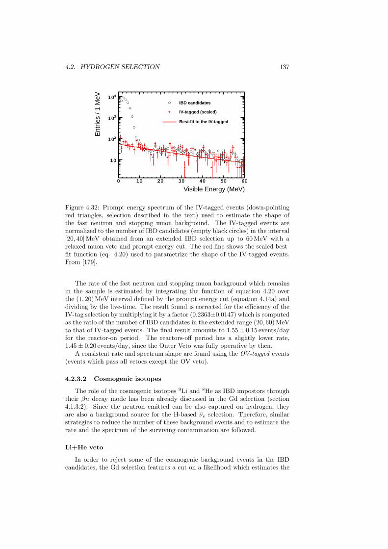
4.2. HYDROGEN SELECTION 137
Visible Energy (MeV)0 10 20 30 40 50 60
Ent
ries
/ 1 M
eV
10
210
310
410IBD candidates
IV-tagged (scaled)
Best-fit to the IV-tagged
Figure 4.32: Prompt energy spectrum of the IV-tagged events (down-pointingred triangles, selection described in the text) used to estimate the shape ofthe fast neutron and stopping muon background. The IV-tagged events arenormalized to the number of IBD candidates (empty black circles) in the interval[20, 40] MeV obtained from an extended IBD selection up to 60 MeV with arelaxed muon veto and prompt energy cut. The red line shows the scaled best-fit function (eq. 4.20) used to parametrize the shape of the IV-tagged events.From [179].
The rate of the fast neutron and stopping muon background which remainsin the sample is estimated by integrating the function of equation 4.20 overthe (1, 20) MeV interval defined by the prompt energy cut (equation 4.14a) anddividing by the live-time. The result found is corrected for the efficiency of theIV-tag selection by multiplying it by a factor (0.2363±0.0147) which is computedas the ratio of the number of IBD candidates in the extended range (20, 60) MeVto that of IV-tagged events. The final result amounts to 1.55± 0.15 events/dayfor the reactor-on period. The reactors-off period has a slightly lower rate,1.45± 0.20 events/day, since the Outer Veto was fully operative by then.
A consistent rate and spectrum shape are found using the OV-tagged events(events which pass all vetoes except the OV veto).
4.2.3.2 Cosmogenic isotopes
The role of the cosmogenic isotopes 9Li and 8He as IBD impostors throughtheir βn decay mode has been already discussed in the Gd selection (section4.1.3.2). Since the neutron emitted can be also captured on hydrogen, theyare also a background source for the H-based νe selection. Therefore, similarstrategies to reduce the number of these background events and to estimate therate and the spectrum of the surviving contamination are followed.
Li+He veto
In order to reject some of the cosmogenic background events in the IBDcandidates, the Gd selection features a cut on a likelihood which estimates the
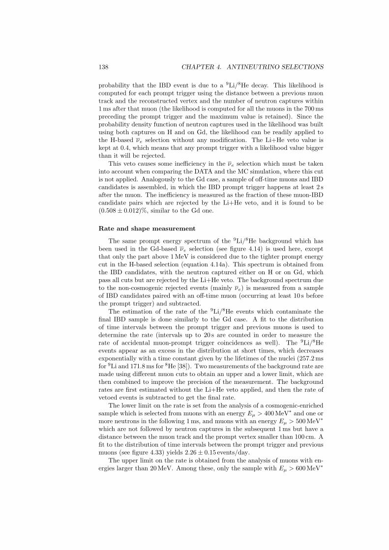
138 CHAPTER 4. ANTINEUTRINO SELECTIONS
probability that the IBD event is due to a 9Li/8He decay. This likelihood iscomputed for each prompt trigger using the distance between a previous muontrack and the reconstructed vertex and the number of neutron captures within1 ms after that muon (the likelihood is computed for all the muons in the 700 mspreceding the prompt trigger and the maximum value is retained). Since theprobability density function of neutron captures used in the likelihood was builtusing both captures on H and on Gd, the likelihood can be readily applied tothe H-based νe selection without any modification. The Li+He veto value iskept at 0.4, which means that any prompt trigger with a likelihood value biggerthan it will be rejected.
This veto causes some inefficiency in the νe selection which must be takeninto account when comparing the DATA and the MC simulation, where this cutis not applied. Analogously to the Gd case, a sample of off-time muons and IBDcandidates is assembled, in which the IBD prompt trigger happens at least 2 safter the muon. The inefficiency is measured as the fraction of these muon-IBDcandidate pairs which are rejected by the Li+He veto, and it is found to be(0.508± 0.012)%, similar to the Gd one.
Rate and shape measurement
The same prompt energy spectrum of the 9Li/8He background which hasbeen used in the Gd-based νe selection (see figure 4.14) is used here, exceptthat only the part above 1 MeV is considered due to the tighter prompt energycut in the H-based selection (equation 4.14a). This spectrum is obtained fromthe IBD candidates, with the neutron captured either on H or on Gd, whichpass all cuts but are rejected by the Li+He veto. The background spectrum dueto the non-cosmogenic rejected events (mainly νe) is measured from a sampleof IBD candidates paired with an off-time muon (occurring at least 10 s beforethe prompt trigger) and subtracted.
The estimation of the rate of the 9Li/8He events which contaminate thefinal IBD sample is done similarly to the Gd case. A fit to the distributionof time intervals between the prompt trigger and previous muons is used todetermine the rate (intervals up to 20 s are counted in order to measure therate of accidental muon-prompt trigger coincidences as well). The 9Li/8Heevents appear as an excess in the distribution at short times, which decreasesexponentially with a time constant given by the lifetimes of the nuclei (257.2 msfor 9Li and 171.8 ms for 8He [38]). Two measurements of the background rate aremade using different muon cuts to obtain an upper and a lower limit, which arethen combined to improve the precision of the measurement. The backgroundrates are first estimated without the Li+He veto applied, and then the rate ofvetoed events is subtracted to get the final rate.
The lower limit on the rate is set from the analysis of a cosmogenic-enrichedsample which is selected from muons with an energy Eµ > 400 MeV∗ and one ormore neutrons in the following 1 ms, and muons with an energy Eµ > 500 MeV∗
which are not followed by neutron captures in the subsequent 1 ms but have adistance between the muon track and the prompt vertex smaller than 100 cm. Afit to the distribution of time intervals between the prompt trigger and previousmuons (see figure 4.33) yields 2.26± 0.15 events/day.
The upper limit on the rate is obtained from the analysis of muons with en-ergies larger than 20 MeV. Among these, only the sample with Eµ > 600 MeV∗
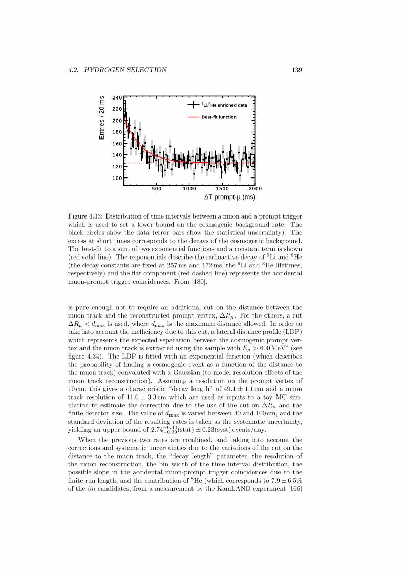
4.2. HYDROGEN SELECTION 139
(ms)µT prompt-∆500 1000 1500 2000
Ent
ries
/ 20
ms
100
120
140
160
180
200
220
240
He enriched data8Li/9
Best-fit function
Figure 4.33: Distribution of time intervals between a muon and a prompt triggerwhich is used to set a lower bound on the cosmogenic background rate. Theblack circles show the data (error bars show the statistical uncertainty). Theexcess at short times corresponds to the decays of the cosmogenic background.The best-fit to a sum of two exponential functions and a constant term is shown(red solid line). The exponentials describe the radioactive decay of 9Li and 8He(the decay constants are fixed at 257 ms and 172 ms, the 9Li and 8He lifetimes,respectively) and the flat component (red dashed line) represents the accidentalmuon-prompt trigger coincidences. From [180].
is pure enough not to require an additional cut on the distance between themuon track and the reconstructed prompt vertex, ∆Rµ. For the others, a cut∆Rµ < dmax is used, where dmax is the maximum distance allowed. In order totake into account the inefficiency due to this cut, a lateral distance profile (LDP)which represents the expected separation between the cosmogenic prompt ver-tex and the muon track is extracted using the sample with Eµ > 600 MeV∗ (seefigure 4.34). The LDP is fitted with an exponential function (which describesthe probability of finding a cosmogenic event as a function of the distance tothe muon track) convoluted with a Gaussian (to model resolution effects of themuon track reconstruction). Assuming a resolution on the prompt vertex of10 cm, this gives a characteristic “decay length” of 49.1 ± 1.1 cm and a muontrack resolution of 11.0 ± 3.3 cm which are used as inputs to a toy MC sim-ulation to estimate the correction due to the use of the cut on ∆Rµ and thefinite detector size. The value of dmax is varied between 40 and 100 cm, and thestandard deviation of the resulting rates is taken as the systematic uncertainty,yielding an upper bound of 2.74+0.43
−0.39(stat)± 0.23(syst) events/day.When the previous two rates are combined, and taking into account the
corrections and systematic uncertainties due to the variations of the cut on thedistance to the muon track, the “decay length” parameter, the resolution ofthe muon reconstruction, the bin width of the time interval distribution, thepossible slope in the accidental muon-prompt trigger coincidences due to thefinite run length, and the contribution of 8He (which corresponds to 7.9± 6.5%of the βn candidates, from a measurement by the KamLAND experiment [166]
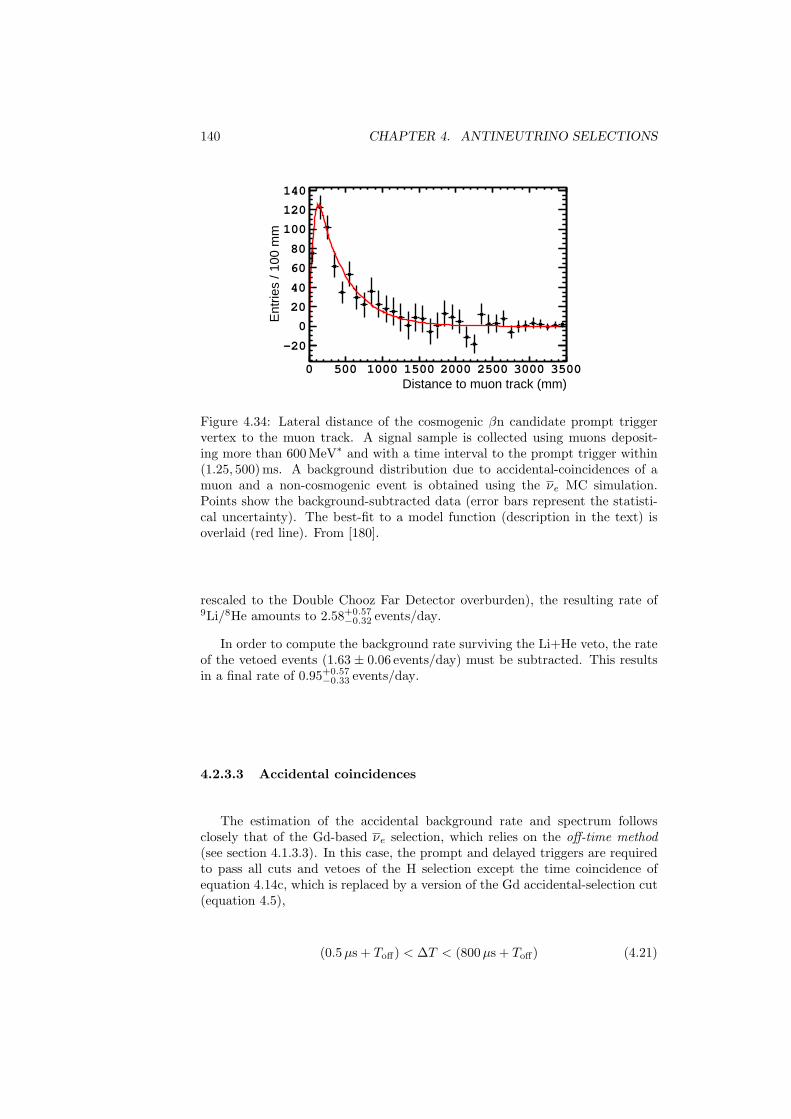
140 CHAPTER 4. ANTINEUTRINO SELECTIONS
Distance to muon track (mm)0 500 1000 1500 2000 2500 3000 3500
Ent
ries
/ 100
mm
-20
0
20
40
60
80
100
120
140
Figure 4.34: Lateral distance of the cosmogenic βn candidate prompt triggervertex to the muon track. A signal sample is collected using muons deposit-ing more than 600 MeV∗ and with a time interval to the prompt trigger within(1.25, 500) ms. A background distribution due to accidental-coincidences of amuon and a non-cosmogenic event is obtained using the νe MC simulation.Points show the background-subtracted data (error bars represent the statisti-cal uncertainty). The best-fit to a model function (description in the text) isoverlaid (red line). From [180].
rescaled to the Double Chooz Far Detector overburden), the resulting rate of9Li/8He amounts to 2.58+0.57
−0.32 events/day.
In order to compute the background rate surviving the Li+He veto, the rateof the vetoed events (1.63 ± 0.06 events/day) must be subtracted. This resultsin a final rate of 0.95+0.57
−0.33 events/day.
4.2.3.3 Accidental coincidences
The estimation of the accidental background rate and spectrum followsclosely that of the Gd-based νe selection, which relies on the off-time method(see section 4.1.3.3). In this case, the prompt and delayed triggers are requiredto pass all cuts and vetoes of the H selection except the time coincidence ofequation 4.14c, which is replaced by a version of the Gd accidental-selection cut(equation 4.5),
(0.5µs + Toff) < ∆T < (800µs + Toff) (4.21)
4.2. HYDROGEN SELECTION 141
where the maximum time has been updated to the value used in the H selection6.Again, the isolation cut (equation 4.14f) must be split into two cuts
No valid triggers in the 800µs beforeand in the 900µs after the prompt. (4.22a)No valid triggers in the 800µs before the time tprompt + Toff
and only one (the delayed) in the 900µs after it. (4.22b)
These are a version of the Gd ones (equation 4.6) with the values adapted tothe H selection.
The time offset, Toff , is given by the same formula (equation 4.7) as inthe Gd case, but in the H selection the total span of the isolation windowis Tiso = 1700µs. Due to the inclusion of the natural radioactivity in thedelayed energy window, the rate of the accidental background is expected tobe much higher in the H selection, even after the cut on the ANN classifiervalue. Consequently, n is restricted to the interval [0, 199]; so only 200 off-timewindows (instead of the 2000 of the Gd) are sufficient to collect the desiredstatistics.
As in the Gd estimation, the accidental background rate resulting from theoff-time method must be corrected due to the different effect that some cutshave in the on-time sample. This is achieved through a series of correctionfactors.
Muon veto correction For the same reason explained in the Gd case, themuon veto has a higher probability to reject the delayed trigger in the off-timesample than in the on-time one. To compensate this deficiency, a correctionfactor, fµ, is computed as the ratio of the probabilities of non-vetoing the delayedtrigger in the on-time and off-time samples, P on
µ and P offµ , respectively (removing
first the events in which the muon veto rejects the prompt trigger too). So far,the procedure is identical to the Gd selection. However, unlike the Gd accidentalbackground, in which the distribution of time intervals between triggers is flat(characteristic of random coincidences); the cut on the ANN classifier outputmakes this distribution non-flat in the H selection (see figure 4.25). While thishas no effect on the off-time probability, which simply requires the delayedtrigger to be preceded by a muon-free window as long as the muon veto time(see equation 4.8c, with Tµ = 1.25 ms); the non-flatness changes the on-timeprobability, in which the probability of a muon-free window is averaged over allthe possible time intervals between the prompt and delayed triggers. Therefore,the expression of the P on
µ probability derived for the Gd case (equation 4.8b) ismodified to
P onµ =
∆Tmax∫∆Tmin
f(t′)e−Rµt′dt′
∆Tmax∫∆Tmin
f(t′)dt′
(4.23)
6In order to make it equivalent to the on-time selection, the time interval between promptand delayed triggers which is fed to the ANN classifier has the time offset subtracted: ∆T −Toff .
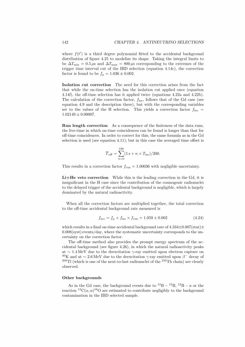
142 CHAPTER 4. ANTINEUTRINO SELECTIONS
where f(t′) is a third degree polynomial fitted to the accidental backgrounddistribution of figure 4.25 to modelize its shape. Taking the integral limits tobe ∆Tmin = 0.5µs and ∆Tmax = 800µs corresponding to the extremes of thetrigger time interval cut of the IBD selection (equation 4.14c), the correctionfactor is found to be fµ = 1.036± 0.002.
Isolation cut correction The need for this correction arises from the factthat while the on-time selection has the isolation cut applied once (equation4.14f), the off-time selection has it applied twice (equations 4.22a and 4.22b).The calculation of the correction factor, fiso, follows that of the Gd case (seeequation 4.9 and the description there), but with the corresponding variablesset to the values of the H selection. This yields a correction factor fiso =1.02149± 0.00007.
Run length correction As a consequence of the finiteness of the data runs,the live-time in which on-time coincidences can be found is longer than that foroff-time coincidences. In order to correct for this, the same formula as in the Gdselection is used (see equation 4.11); but in this case the averaged time offset is
T off =199∑n=0
(1 s + n× Tiso)/200.
This results in a correction factor frun = 1.00036 with negligible uncertainty.
Li+He veto correction While this is the leading correction in the Gd, it isinsignificant in the H case since the contribution of the cosmogenic radionucleito the delayed trigger of the accidental background is negligible, which is largelydominated by the natural radioactivity.
When all the correction factors are multiplied together, the total correctionto the off-time accidental background rate measured is
facc = fµ × fiso × frun = 1.059± 0.002 (4.24)
which results in a final on-time accidental background rate of 4.334±0.007(stat)±0.008(syst) events/day, where the systematic uncertainty corresponds to the un-certainty on the correction factor.
The off-time method also provides the prompt energy spectrum of the ac-cidental background (see figure 4.26), in which the natural radioactivity peaksat ∼ 1.4 MeV due to the deexcitation γ-ray emitted upon electron capture on40K and at ∼ 2.6 MeV due to the deexcitation γ-ray emitted upon β− decay of208Tl (which is one of the next-to-last radionuclei of the 232Th chain) are clearlyobserved.
Other backgrounds
As in the Gd case, the background events due to 12B− 12B, 12B− n or thereaction 13C(α,n)16O are estimated to contribute negligibly to the backgroundcontamination in the IBD selected sample.
4.2. HYDROGEN SELECTION 143
Event type Rate (events/day) H-III/H-II
IBD candidates (average) 69.88± 0.39 —Backgrounds
Fast-n and stopping-µ 1.55± 0.15 0.499Li and 8He 0.95+0.57
−0.33 0.34Accidental 4.334±0.0007(stat)
±0.0008(syst) 0.06
Table 4.4: Summary of the rates of the events passing the H-based νe selection.The IBD candidate (including backgrounds) average rate during the periodswith at least one reactor on is shown; the actual IBD rate changes in time as afunction of the thermal power of the reactors as in equation 2.7. The backgroundrates correspond to the expected rates remaining in the IBD candidate sampleafter the full νe selection is performed, estimated from samples rejected byit as explained in the text. The column H-III/H-II shows the reduction ofthe background rate in the current selection [159] with respect to the previouspublication [72].
When this thesis was being finalized, an additional background contributiondue to double neutron captures on H was found. This background is createdwhen two spallation neutrons created outside the detector manage to reach theGamma Catcher and mimic an IBD coincidence there, without revealing theirpresence first through an energetic proton recoil in the Inner Veto, which couldreject the coincidence because of the IV veto explained in section 4.2.3.1; or aproton recoil in the Inner Detector, which could make them to be rejected bythe isolation cut in equation 4.14f. In the latter case, it must be noted that theisolation cut is only applied over valid triggers (i.e. not within the 1.25µs aftera muon, not tagged as light noise, with an energy larger than 0.4 MeV). Thisopens the possibility to avoid the rejection by the isolation cut if the protonrecoil occurs in the time still vetoed by the muon veto window, or if the protonrecoil looks like a light noise event (e.g. if it happens very close to a PMT) orif it has an energy below 0.4 MeV. In all this cases, what would have been arejected triple coincidence becomes an acceptable IBD-like coincidence.
Studying triple coincidences in which the first trigger is deemed invalid forthe abovesaid reasons, and after correction for the efficiency of detecting this firsttrigger, the rate of this background was estimated to be 0.15+0.05
−0.04 events/day.Given that the rate is much lower than the usual background sources alreadyknown (see table 4.4), and since the inclusion of this background in the os-cillation fits of chapter 6 proved that the change on the θ13 measurement isnot significant at all, and the Rate+Shape analysis pulls its rate even to lowervalues, it is not further considered for the rest of the thesis.
4.2.3.4 Reactors-off measurement
When the H-based νe selection is applied to the periods when the two re-actors are off, the data amounts to a live-time of 7.15 days in which 63 IBDcandidates passing all cuts are found. The predicted number of IBD interac-tions due to residual νe from the stopped reactors is 2.73 ± 0.82 according to
144 CHAPTER 4. ANTINEUTRINO SELECTIONS
the simulation [170] (oscillation not included). When the expected number ofIBD background events are included according to their estimated rates, the pre-diction raises to 50.8+4.4
−2.9 events, which agrees within 1.4σ with the observation,demonstrating the consistency of the background estimations.
Chapter 5
Neutron detection efficiency
In the one-detector phase, Double Chooz relies on a Monte Carlo simula-tion to predict the νe flux at the Far Detector which will be compared to theDATA to measure the oscillation-induced deficit. Therefore, the accuracy ofthe simulation in reproducing the νe generation and detection is mandatory inthis phase of the experiment. The νe detection efficiency is one of the vari-ables of the simulation that must be ensured to match the one in the actualDATA. However, because either certain effects are not included or they are notwell reproduced in the simulation, the normalization of the prediction must becorrected a posteriori, which adds an additional uncertainty source.
This chapter is dedicated to the detection efficiency of the neutron producedin the inverse β-decay: its measurement, determination of its correction factorand uncertainty. The motivation for an in-depth study results from the neu-tron detection efficiency being the dominant contribution to the νe detectionuncertainty in the Double Chooz θ13 measurements [69, 1].
The structure of the chapter is as follows: firstly, the νe detection efficiencyand the factor used to correct the Monte Carlo simulation to meet the observeddate are introduced in section 5.1. Secondly, a synopsis on how the neutronphysics is simulated in Double Chooz is presented in section 5.2, which helpsto underline the difficulties associated to it. Thirdly, the two neutron sourcesused for the studies are described in section 5.3. Then, the study of the neutrondetection efficiency bifurcates corresponding to the two νe selections developed,the one using neutron captures on gadolinium and the one using the captures onhydrogen, which are presented sequentially in sections 5.4 and 5.5. For each one,the three components in which the neutron detection efficiency is decomposedare discussed thoroughly.
5.1 Monte Carlo correction factor
The antineutrinos emitted by the two cores of the Chooz nuclear power plantare detected through the inverse β-decay reaction: νe + p → e+ + n. As seenin chapter 2, in the null-oscillation hypothesis, the expected rate of νe from areactor R detected in one detector through the IBD reaction at time t is given
145
146 CHAPTER 5. NEUTRON DETECTION EFFICIENCY
by:dNR(t)
dt= εNp
[1
4πL2R
Pth,R(t)〈Ef〉R(t)
〈σf〉R(t)], (5.1)
where ε denotes the νe detection efficiency andNp denotes the number of protonsin the detector considered. The remaining variables between the square bracketsare reactor-related and they have been discussed in section 2.4.1.
The Double Chooz MC simulation is designed to replicate step by step theDATA, from the generation of νe in the reactor to their interaction in the de-tector, including the posterior conversion of the event into numerical variablesthat are used in the selection. Thus, DATA and MC are analyzed in an identicalway. This means that there is already a built-in detection efficiency in the MCsimulation, εMC, which can be identified with the ε in equation 5.1. However, inorder to make the simulation outcome comparable to the actual DATA whichhas its own detection efficiency, εDATA, εMC must be corrected to account forknown effects which have not been included in the simulation or for shortcom-ings in the modeling. This is achieved using a MC normalization correctionfactor, cMC which is defined as:
cMC ≡εDATA
εMC. (5.2)
Notice that, because cMC is defined as the ratio of the two efficiencies, they donot need to be absolute efficiencies (i.e. the fraction of selected νe with respectto the total number of νe that interacted in the detector), which in the caseof the DATA is impossible to know, but they can be relative efficiencies, thatis, the fraction of νe passing the selection cuts with respect to a parent samplewhich satisfies looser cuts.
The signal detection efficiency can be factorized into three components cor-responding to the selection steps followed in the search for IBD events: firstassemble a set of valid triggers (singles), and then look for coincidences of aprompt and a delayed trigger:
ε ≡ εsingle · εprompt · εdelayed. (5.3)
Each factor can be further decomposed into the intrinsic sources which causethe inefficiencies:
εsingle ≡ εµ · εLN (5.4)εprompt ≡ εtrig · εiso · εveto (5.5)εdelayed ≡ fX · εsel · kspill. (5.6)
εsingle denotes the efficiency of the single selection and it is divided into twofactors: εµ represents the efficiency of the muon veto and εLN represents theefficiency of the light noise cuts.
The positron detection efficiency, εprompt, consists of three components: εtrigcorresponds to the trigger efficiency. Because the minimum energy of the prompttriggers is set where the trigger has a 100% efficiency with insignificant uncer-tainty, this factor is trivial but it is written for completeness. εiso correspondsto the efficiency of the isolation cut. εveto corresponds to the total efficiency of
5.2. NEUTRON PHYSICS SIMULATION 147
the background vetoes: Li+He, OV, IV, FV 1 and MPS (only in the H analysis).The neutron detection efficiency, εdelayed, is factorized into three components:
the gadolinium or hydrogen fraction (depending on the nuclei used to capture theneutron) fX , where X denotes Gd or H, a neutron selection efficiency, εsel, anda neutron mobility factor, kspill. There is no need to include a trigger efficiencyfactor in εdelayed because, regardless the nucleus used to capture the neutron,the energy interval begins when the trigger is 100% efficient with negligibleuncertainty.
The MC normalization correction factor, cMC, can be factorized analogouslyas the signal detection efficiency.
cMC ≡ csingle · cprompt · cdelayed, (5.7)
where:
csingle ≡ cµ · cLN (5.8)cprompt ≡ ctrig · ciso · cveto (5.9)cdelayed ≡ cX · csel · cspill. (5.10)
Since the MC simulation used for the prediction contains exclusively electronantineutrino IBD interactions; the muon, light noise, isolation and backgroundveto cuts are unnecessary and not applied to it. Therefore, the expected νenumber must be corrected to account for the inefficiencies in the DATA νeselection caused by these cuts. The computation of the inefficiencies and theiruncertainty has already been described in chapter 4. The results are summarizedin tables 4.1 (Gd selection) and 4.3 (H selection).
Regarding the neutron detection efficiency, it is the subject of this chapter.Since the detailed explanation of each component and the methods used to mea-sure them and compute their correction factors and uncertainties are dependenton the nuclei used to capture the neutron, they are given in the dedicated sectionof each analysis.
5.2 Neutron physics simulation
The neutron detection efficiency correction (eq. 5.10) originates from dis-crepancies between the DATA and the MC simulation regarding the neutronphysics. Therefore, before discussing how this correction is calculated, it is use-ful to describe briefly the simulation of the neutron physics in Double Chooz.
The νe generator, DCRxtrTools [145], also generates the neutron in thedetector with the corresponding momentum according to the IBD kinematics[123]. Then, the interaction with the detector components is simulated usingthe Geant4-based software, DCGLG4sim (section 2.4.2), in which the detectorgeometry and materials have been implemented.
The neutron resulting from an IBD interaction is produced with a kineticenergy in the range of tens of keV, which is quickly reduced mainly by elasticscattering off protons (H nuclei, which have a relative abundance of 65.3% in the
1Although the FV veto uses delayed variables, and in the H analysis there is also a IV vetoto the delayed trigger, they are grouped together with the other background vetoes on theprompt trigger for clarity and because they do not rely on the neutron physics modelization.
148 CHAPTER 5. NEUTRON DETECTION EFFICIENCY
Target and 67% in the Gamma Catcher scintillators [181]). The loss of the neu-tron kinetic energy in these elastic scatterings is initially very efficient becausethe neutron and proton masses are similar, and the protons can be considered atrest. When the neutron approaches the thermal regime, protons can no longerbe considered at rest, and the thermalization process is characterized by a timeconstant O(µs).
When the neutron kinetic energy falls below 4 eV, the interaction with H nu-clei, which so far has been simulated using Geant4’s NeutronHPElastic (whichtreats the H nuclei as a free gas of protons), is substituted with the modelused in NeutronTH. NeutronTH is the Double Chooz custom implementation ofthe low energy neutron scattering [182, 183] and is based on the parametriza-tion of experimental data following the effective analytical model of reference[184], which takes into account the effect of the molecular bounds, which cannotbe neglected anymore since the neutron energies are of the same order as themolecular binding energies. This causes a rise in the cross section and makes theenergy loss mechanism to become less efficient, since the neutron interacts withthe whole molecule rather than with a single H nucleus. The increase in the crosssection, which also changes the angular distribution of the scattered neutron,decreases the neutron mean free path, causing the ∆R (cf. figure 4.8) distribu-tion to fall faster. The molecular bonds are modeled as in dodecane, which isa representative molecule since dodecane and dodecane-like molecules are themajor constituents of the scintillator. When the neutron is finally thermalized,the capture is governed by a diffusion process in which the characteristic timedepends on the scintillator considered: ∼ 30µs for the Target and ∼ 200µs forthe Gamma Catcher. In figure 5.1, the radiative neutron capture cross section isshown as a function of the neutron kinetic energy for the two Gd isotopes withthe largest cross section, 157Gd and 155Gd (which have an isotopic abundanceof 15.7% and 14.8%, respectively), together with the ones for 12C and 1H. Sincethe cross section is inversely proportional to the neutron energy, the increase inits recoil energy caused by taking into consideration the H molecular bounds istranslated into a longer neutron capture time, which shifts the maximum of the∆T distribution (cf. figure 4.7) to higher values.
Eventually, the neutron will be captured. A thermal neutron (kinetic energy∼ 0.03 eV) within the Target will be preferentially captured on a Gd nucleusas a result of the higher cross section (2.54 · 105 b for 157Gd, 6.09 · 104 b for155Gd), or on a 1H nucleus in which the lower cross section (0.33 b) is partiallycompensated with its larger relative abundance NH/NGd = 1.72·104; whereas inthe Gamma Catcher, the neutron will be almost exclusively captured on H. Thecapture on 1H yields a single γ ray with an energy of 2.22 MeV, and the captureon Gd yields multiple γ rays totaling ∼ 8 MeV. The energy distribution of theseγ rays depends on the structure of the energy levels of the Gd nucleus whichcaptured the neutron, which are populated differently according to the neutronincident energy. This is specially relevant for neutron energies below 300 eV, forwhich gadolinium exhibits resonances in the capture cross section (see fig. 5.1)corresponding to different structures of excited levels. NeutronTH takes thisinto consideration by substituting the Geant4 distribution of γ rays which isused above that energy with an experimental γ ray emission spectrum from theENSDF database (see figure 5.2) which is used as a proxy for all the energies below300 eV, since the lack of data and the small variations for low energy neutronsdo not advocate a more complex treatment. Despite the radiative capture on
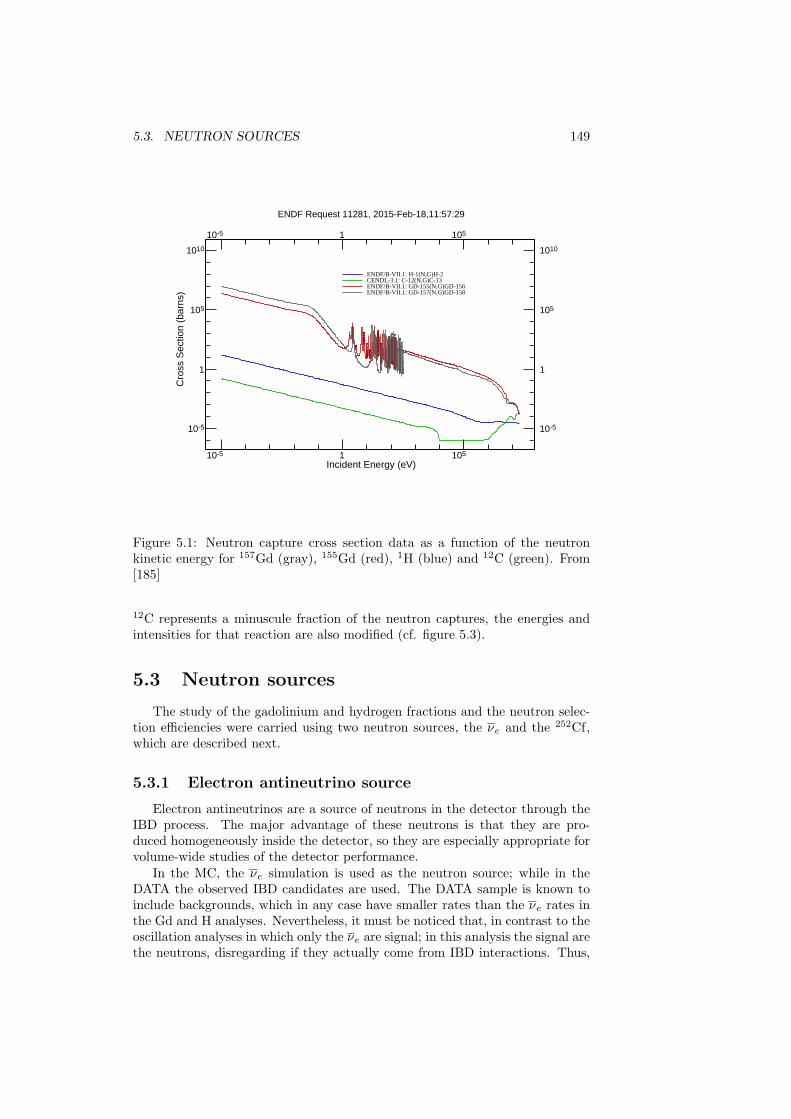
5.3. NEUTRON SOURCES 149
ENDF Request 11281, 2015-Feb-18,11:57:29
Incident Energy (eV)
Cro
ss S
ectio
n (b
arns
)
10-5 1 105
10-5
1
105
1010
10-5
1
105
1010
10-5 1 105
ENDF/B-VII.1: H-1(N,G)H-2CENDL-3.1: C-12(N,G)C-13ENDF/B-VII.1: GD-155(N,G)GD-156ENDF/B-VII.1: GD-157(N,G)GD-158
Figure 5.1: Neutron capture cross section data as a function of the neutronkinetic energy for 157Gd (gray), 155Gd (red), 1H (blue) and 12C (green). From[185]
12C represents a minuscule fraction of the neutron captures, the energies andintensities for that reaction are also modified (cf. figure 5.3).
5.3 Neutron sources
The study of the gadolinium and hydrogen fractions and the neutron selec-tion efficiencies were carried using two neutron sources, the νe and the 252Cf,which are described next.
5.3.1 Electron antineutrino source
Electron antineutrinos are a source of neutrons in the detector through theIBD process. The major advantage of these neutrons is that they are pro-duced homogeneously inside the detector, so they are especially appropriate forvolume-wide studies of the detector performance.
In the MC, the νe simulation is used as the neutron source; while in theDATA the observed IBD candidates are used. The DATA sample is known toinclude backgrounds, which in any case have smaller rates than the νe rates inthe Gd and H analyses. Nevertheless, it must be noticed that, in contrast to theoscillation analyses in which only the νe are signal; in this analysis the signal arethe neutrons, disregarding if they actually come from IBD interactions. Thus,
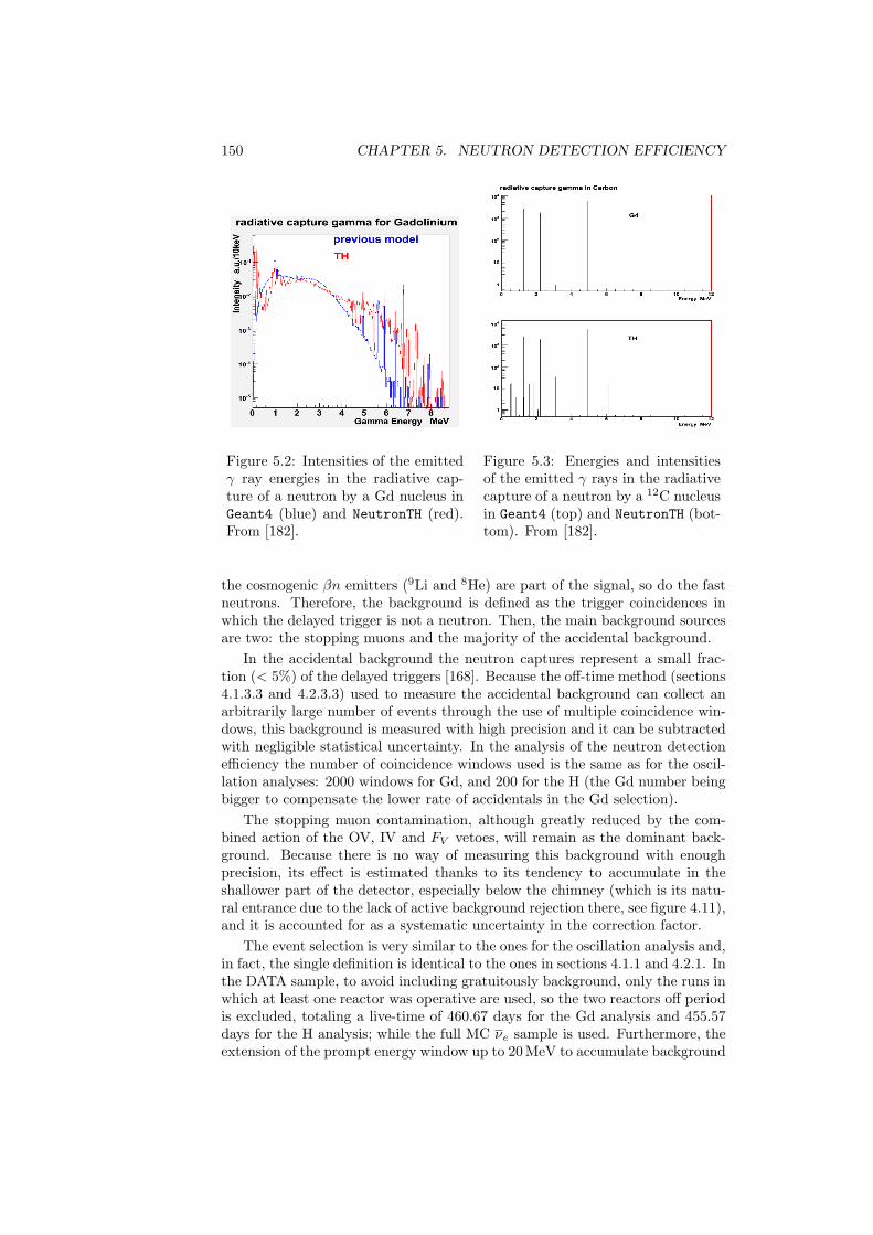
150 CHAPTER 5. NEUTRON DETECTION EFFICIENCY
Figure 5.2: Intensities of the emittedγ ray energies in the radiative cap-ture of a neutron by a Gd nucleus inGeant4 (blue) and NeutronTH (red).From [182].
Figure 5.3: Energies and intensitiesof the emitted γ rays in the radiativecapture of a neutron by a 12C nucleusin Geant4 (top) and NeutronTH (bot-tom). From [182].
the cosmogenic βn emitters (9Li and 8He) are part of the signal, so do the fastneutrons. Therefore, the background is defined as the trigger coincidences inwhich the delayed trigger is not a neutron. Then, the main background sourcesare two: the stopping muons and the majority of the accidental background.
In the accidental background the neutron captures represent a small frac-tion (< 5%) of the delayed triggers [168]. Because the off-time method (sections4.1.3.3 and 4.2.3.3) used to measure the accidental background can collect anarbitrarily large number of events through the use of multiple coincidence win-dows, this background is measured with high precision and it can be subtractedwith negligible statistical uncertainty. In the analysis of the neutron detectionefficiency the number of coincidence windows used is the same as for the oscil-lation analyses: 2000 windows for Gd, and 200 for the H (the Gd number beingbigger to compensate the lower rate of accidentals in the Gd selection).
The stopping muon contamination, although greatly reduced by the com-bined action of the OV, IV and FV vetoes, will remain as the dominant back-ground. Because there is no way of measuring this background with enoughprecision, its effect is estimated thanks to its tendency to accumulate in theshallower part of the detector, especially below the chimney (which is its natu-ral entrance due to the lack of active background rejection there, see figure 4.11),and it is accounted for as a systematic uncertainty in the correction factor.
The event selection is very similar to the ones for the oscillation analysis and,in fact, the single definition is identical to the ones in sections 4.1.1 and 4.2.1. Inthe DATA sample, to avoid including gratuitously background, only the runs inwhich at least one reactor was operative are used, so the two reactors off periodis excluded, totaling a live-time of 460.67 days for the Gd analysis and 455.57days for the H analysis; while the full MC νe sample is used. Furthermore, theextension of the prompt energy window up to 20 MeV to accumulate background
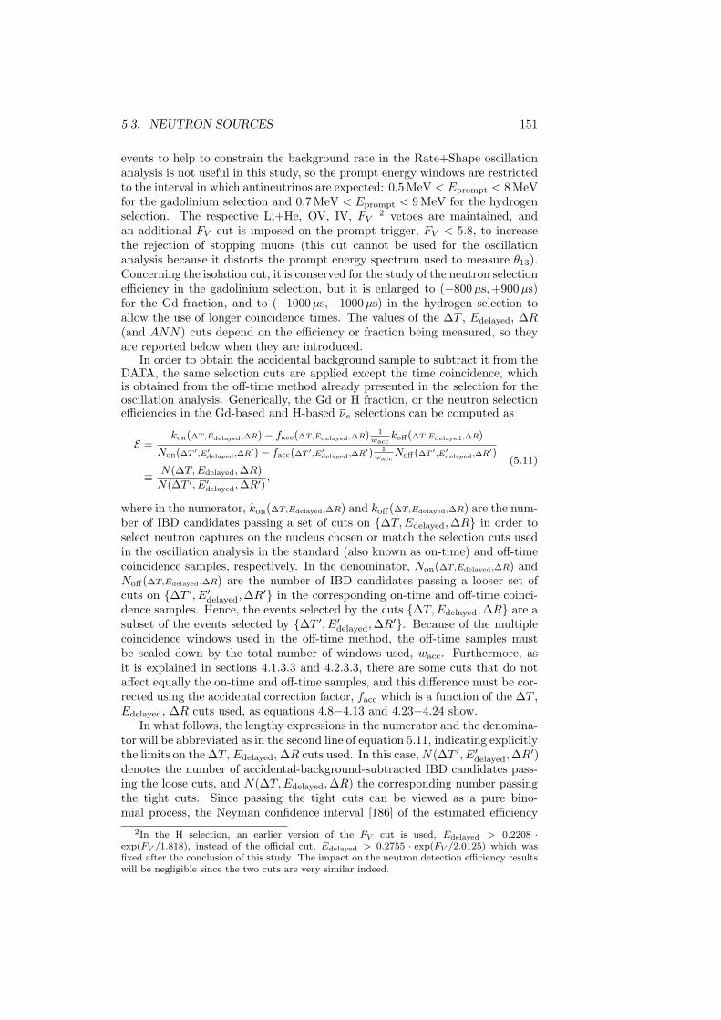
5.3. NEUTRON SOURCES 151
events to help to constrain the background rate in the Rate+Shape oscillationanalysis is not useful in this study, so the prompt energy windows are restrictedto the interval in which antineutrinos are expected: 0.5 MeV < Eprompt < 8 MeVfor the gadolinium selection and 0.7 MeV < Eprompt < 9 MeV for the hydrogenselection. The respective Li+He, OV, IV, FV 2 vetoes are maintained, andan additional FV cut is imposed on the prompt trigger, FV < 5.8, to increasethe rejection of stopping muons (this cut cannot be used for the oscillationanalysis because it distorts the prompt energy spectrum used to measure θ13).Concerning the isolation cut, it is conserved for the study of the neutron selectionefficiency in the gadolinium selection, but it is enlarged to (−800µs,+900µs)for the Gd fraction, and to (−1000µs,+1000µs) in the hydrogen selection toallow the use of longer coincidence times. The values of the ∆T , Edelayed, ∆R(and ANN) cuts depend on the efficiency or fraction being measured, so theyare reported below when they are introduced.
In order to obtain the accidental background sample to subtract it from theDATA, the same selection cuts are applied except the time coincidence, whichis obtained from the off-time method already presented in the selection for theoscillation analysis. Generically, the Gd or H fraction, or the neutron selectionefficiencies in the Gd-based and H-based νe selections can be computed as
E =kon(∆T,Edelayed,∆R)− facc(∆T,Edelayed,∆R) 1
wacckoff(∆T,Edelayed,∆R)
Non(∆T ′,E′delayed,∆R′)− facc(∆T ′,E′delayed,∆R
′) 1wacc
Noff(∆T ′,E′delayed,∆R′)
≡ N(∆T,Edelayed,∆R)
N(∆T ′, E′delayed,∆R′),
(5.11)
where in the numerator, kon(∆T,Edelayed,∆R) and koff(∆T,Edelayed,∆R) are the num-ber of IBD candidates passing a set of cuts on ∆T,Edelayed,∆R in order toselect neutron captures on the nucleus chosen or match the selection cuts usedin the oscillation analysis in the standard (also known as on-time) and off-timecoincidence samples, respectively. In the denominator, Non(∆T,Edelayed,∆R) andNoff(∆T,Edelayed,∆R) are the number of IBD candidates passing a looser set ofcuts on ∆T ′, E′delayed,∆R
′ in the corresponding on-time and off-time coinci-dence samples. Hence, the events selected by the cuts ∆T,Edelayed,∆R are asubset of the events selected by ∆T ′, E′delayed,∆R
′. Because of the multiplecoincidence windows used in the off-time method, the off-time samples mustbe scaled down by the total number of windows used, wacc. Furthermore, asit is explained in sections 4.1.3.3 and 4.2.3.3, there are some cuts that do notaffect equally the on-time and off-time samples, and this difference must be cor-rected using the accidental correction factor, facc which is a function of the ∆T ,Edelayed, ∆R cuts used, as equations 4.8−4.13 and 4.23−4.24 show.
In what follows, the lengthy expressions in the numerator and the denomina-tor will be abbreviated as in the second line of equation 5.11, indicating explicitlythe limits on the ∆T , Edelayed, ∆R cuts used. In this case, N(∆T ′, E′delayed,∆R
′)denotes the number of accidental-background-subtracted IBD candidates pass-ing the loose cuts, and N(∆T,Edelayed,∆R) the corresponding number passingthe tight cuts. Since passing the tight cuts can be viewed as a pure bino-mial process, the Neyman confidence interval [186] of the estimated efficiency
2In the H selection, an earlier version of the FV cut is used, Edelayed > 0.2208 ·exp(FV /1.818), instead of the official cut, Edelayed > 0.2755 · exp(FV /2.0125) which wasfixed after the conclusion of this study. The impact on the neutron detection efficiency resultswill be negligible since the two cuts are very similar indeed.
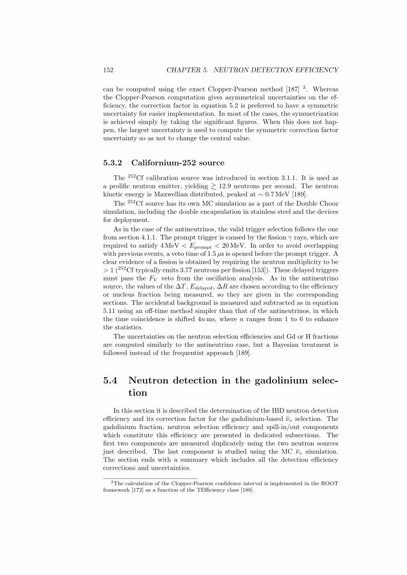
152 CHAPTER 5. NEUTRON DETECTION EFFICIENCY
can be computed using the exact Clopper-Pearson method [187] 3. Whereasthe Clopper-Pearson computation gives asymmetrical uncertainties on the ef-ficiency, the correction factor in equation 5.2 is preferred to have a symmetricuncertainty for easier implementation. In most of the cases, the symmetrizationis achieved simply by taking the significant figures. When this does not hap-pen, the largest uncertainty is used to compute the symmetric correction factoruncertainty so as not to change the central value.
5.3.2 Californium-252 source
The 252Cf calibration source was introduced in section 3.1.1. It is used asa prolific neutron emitter, yielding & 12.9 neutrons per second. The neutronkinetic energy is Maxwellian distributed, peaked at ∼ 0.7 MeV [189].
The 252Cf source has its own MC simulation as a part of the Double Choozsimulation, including the double encapsulation in stainless steel and the devicesfor deployment.
As in the case of the antineutrinos, the valid trigger selection follows the onefrom section 4.1.1. The prompt trigger is caused by the fission γ rays, which arerequired to satisfy 4 MeV < Eprompt < 20 MeV. In order to avoid overlappingwith previous events, a veto time of 1.5µs is opened before the prompt trigger. Aclear evidence of a fission is obtained by requiring the neutron multiplicity to be> 1 (252Cf typically emits 3.77 neutrons per fission [153]). These delayed triggersmust pass the FV veto from the oscillation analysis. As in the antineutrinosource, the values of the ∆T , Edelayed, ∆R are chosen according to the efficiencyor nucleus fraction being measured, so they are given in the correspondingsections. The accidental background is measured and subtracted as in equation5.11 using an off-time method simpler than that of the antineutrinos, in whichthe time coincidence is shifted 4nms, where n ranges from 1 to 6 to enhancethe statistics.
The uncertainties on the neutron selection efficiencies and Gd or H fractionsare computed similarly to the antineutrino case, but a Bayesian treatment isfollowed instead of the frequentist approach [189].
5.4 Neutron detection in the gadolinium selec-tion
In this section it is described the determination of the IBD neutron detectionefficiency and its correction factor for the gadolinium-based νe selection. Thegadolinium fraction, neutron selection efficiency and spill-in/out componentswhich constitute this efficiency are presented in dedicated subsections. Thefirst two components are measured duplicately using the two neutron sourcesjust described. The last component is studied using the MC νe simulation.The section ends with a summary which includes all the detection efficiencycorrections and uncertainties.
3The calculation of the Clopper-Pearson confidence interval is implemented in the ROOTframework [172] as a function of the TEfficiency class [188].
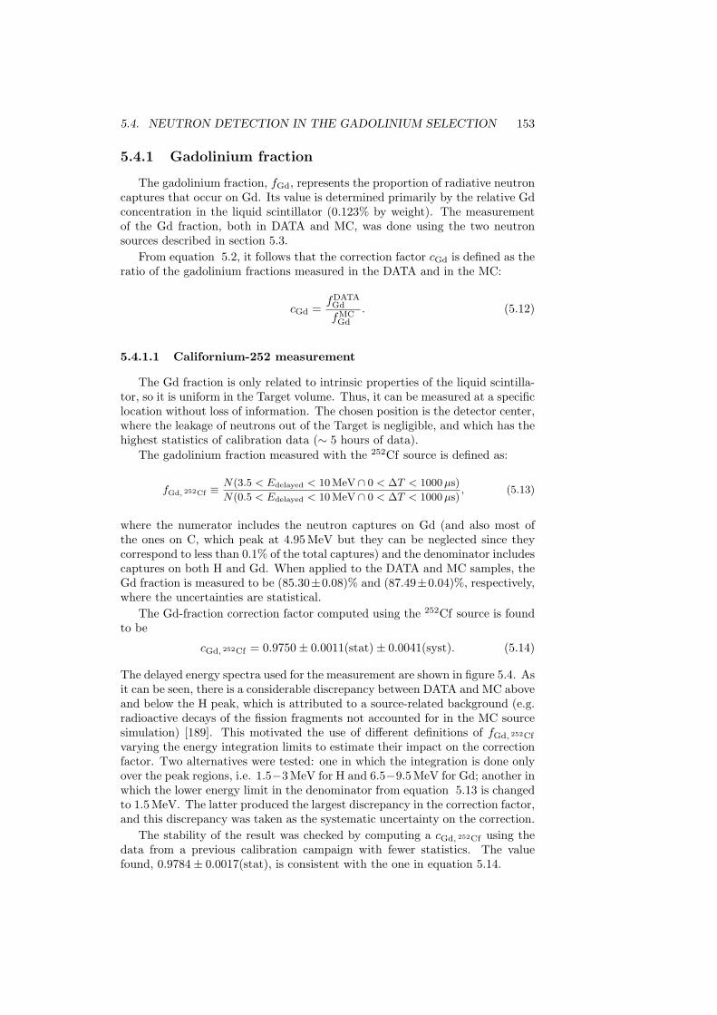
5.4. NEUTRON DETECTION IN THE GADOLINIUM SELECTION 153
5.4.1 Gadolinium fraction
The gadolinium fraction, fGd, represents the proportion of radiative neutroncaptures that occur on Gd. Its value is determined primarily by the relative Gdconcentration in the liquid scintillator (0.123% by weight). The measurementof the Gd fraction, both in DATA and MC, was done using the two neutronsources described in section 5.3.
From equation 5.2, it follows that the correction factor cGd is defined as theratio of the gadolinium fractions measured in the DATA and in the MC:
cGd =fDATA
Gd
fMCGd
. (5.12)
5.4.1.1 Californium-252 measurement
The Gd fraction is only related to intrinsic properties of the liquid scintilla-tor, so it is uniform in the Target volume. Thus, it can be measured at a specificlocation without loss of information. The chosen position is the detector center,where the leakage of neutrons out of the Target is negligible, and which has thehighest statistics of calibration data (∼ 5 hours of data).
The gadolinium fraction measured with the 252Cf source is defined as:
fGd, 252Cf ≡N(3.5 < Edelayed < 10 MeV ∩ 0 < ∆T < 1000µs)
N(0.5 < Edelayed < 10 MeV ∩ 0 < ∆T < 1000µs), (5.13)
where the numerator includes the neutron captures on Gd (and also most ofthe ones on C, which peak at 4.95 MeV but they can be neglected since theycorrespond to less than 0.1% of the total captures) and the denominator includescaptures on both H and Gd. When applied to the DATA and MC samples, theGd fraction is measured to be (85.30±0.08)% and (87.49±0.04)%, respectively,where the uncertainties are statistical.
The Gd-fraction correction factor computed using the 252Cf source is foundto be
cGd, 252Cf = 0.9750± 0.0011(stat)± 0.0041(syst). (5.14)
The delayed energy spectra used for the measurement are shown in figure 5.4. Asit can be seen, there is a considerable discrepancy between DATA and MC aboveand below the H peak, which is attributed to a source-related background (e.g.radioactive decays of the fission fragments not accounted for in the MC sourcesimulation) [189]. This motivated the use of different definitions of fGd, 252Cf
varying the energy integration limits to estimate their impact on the correctionfactor. Two alternatives were tested: one in which the integration is done onlyover the peak regions, i.e. 1.5−3 MeV for H and 6.5−9.5 MeV for Gd; another inwhich the lower energy limit in the denominator from equation 5.13 is changedto 1.5 MeV. The latter produced the largest discrepancy in the correction factor,and this discrepancy was taken as the systematic uncertainty on the correction.
The stability of the result was checked by computing a cGd, 252Cf using thedata from a previous calibration campaign with fewer statistics. The valuefound, 0.9784± 0.0017(stat), is consistent with the one in equation 5.14.
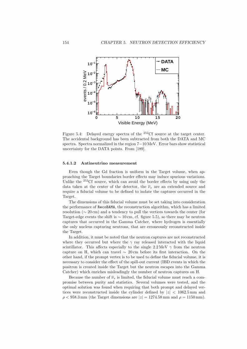
154 CHAPTER 5. NEUTRON DETECTION EFFICIENCY
Visible Energy (MeV)0 5 10 15 20
even
ts /
0.2
MeV
-610
-510
-410
-310
-210
-110 DATA
MC
Figure 5.4: Delayed energy spectra of the 252Cf source at the target center.The accidental background has been subtracted from both the DATA and MCspectra. Spectra normalized in the region 7−10 MeV. Error bars show statisticaluncertainty for the DATA points. From [189].
5.4.1.2 Antineutrino measurement
Even though the Gd fraction is uniform in the Target volume, when ap-proaching the Target boundaries border effects may induce spurious variations.Unlike the 252Cf source, which can avoid the border effects by using only thedata taken at the center of the detector, the νe are an extended source andrequire a fiducial volume to be defined to isolate the captures occurred in theTarget.
The dimensions of this fiducial volume must be set taking into considerationthe performance of RecoBAMA, the reconstruction algorithm, which has a limitedresolution (∼ 20 cm) and a tendency to pull the vertices towards the center (forTarget-edge events the shift is ∼ 10 cm, cf. figure 5.5), so there may be neutroncaptures that occurred in the Gamma Catcher, where hydrogen is essentiallythe only nucleus capturing neutrons, that are erroneously reconstructed insidethe Target.
In addition, it must be noted that the neutron captures are not reconstructedwhere they occurred but where the γ ray released interacted with the liquidscintillator. This affects especially to the single 2.2 MeV γ from the neutroncapture on H, which can travel ∼ 20 cm before its first interaction. On theother hand, if the prompt vertex is to be used to define the fiducial volume, it isnecessary to consider the effect of the spill-out current (IBD events in which thepositron is created inside the Target but the neutron escapes into the GammaCatcher) which enriches misleadingly the number of neutron captures on H.
Because the number of νe is limited, the fiducial volume must reach a com-promise between purity and statistics. Several volumes were tested, and theoptimal solution was found when requiring that both prompt and delayed ver-tices were reconstructed inside the cylinder defined by |z| < 1062.5 mm andρ < 958.3 mm (the Target dimensions are |z| = 1274.58 mm and ρ = 1150 mm).
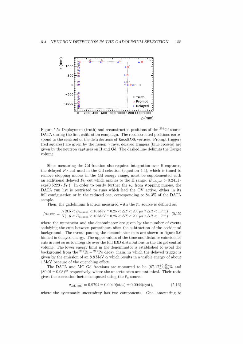
5.4. NEUTRON DETECTION IN THE GADOLINIUM SELECTION 155
(mm)ρ0 200 400 600 800 1000 1200 1400 1600
z (m
m)
-1000
-500
0
500
1000
TruthPromptDelayed
Figure 5.5: Deployment (truth) and reconstructed positions of the 252Cf sourceDATA during the first calibration campaign. The reconstructed positions corre-spond to the centroid of the distributions of RecoBAMA vertices. Prompt triggers(red squares) are given by the fission γ rays, delayed triggers (blue crosses) aregiven by the neutron captures on H and Gd. The dashed line delimits the Targetvolume.
Since measuring the Gd fraction also requires integration over H captures,the delayed FV cut used in the Gd selection (equation 4.4), which is tuned toremove stopping muons in the Gd energy range, must be supplemented withan additional delayed FV cut which applies to the H range: Edelayed > 0.2411 ·exp(0.5223 · FV ). In order to purify further the νe from stopping muons, theDATA run list is restricted to runs which had the OV active, either in itsfull configuration or in the reduced one, corresponding to 84.3% of the DATAsample.
Then, the gadolinium fraction measured with the νe source is defined as:
fGd, IBD ≡N(3.5 < Edelayed < 10 MeV ∩ 0.25 < ∆T < 200µs ∩∆R < 1.7 m)
N(1.6 < Edelayed < 10 MeV ∩ 0.25 < ∆T < 200µs ∩∆R < 1.7 m), (5.15)
where the numerator and the denominator are given by the number of eventssatisfying the cuts between parentheses after the subtraction of the accidentalbackground. The events passing the denominator cuts are shown in figure 5.6binned in delayed energy. The upper values of the time and distance coincidencecuts are set so as to integrate over the full IBD distributions in the Target centralvolume. The lower energy limit in the denominator is established to avoid thebackground from the 212Bi− 212Po decay chain, in which the delayed trigger isgiven by the emission of an 8.8 MeV α which results in a visible energy of about1 MeV because of the quenching effect.
The DATA and MC Gd fractions are measured to be (87.17+0.35−0.36)% and
(89.01± 0.03)% respectively, where the uncertainties are statistical. Their ratiogives the correction factor computed using the νe source:
cGd, IBD = 0.9794± 0.0040(stat)± 0.0044(syst), (5.16)
where the systematic uncertainty has two components. One, amounting to
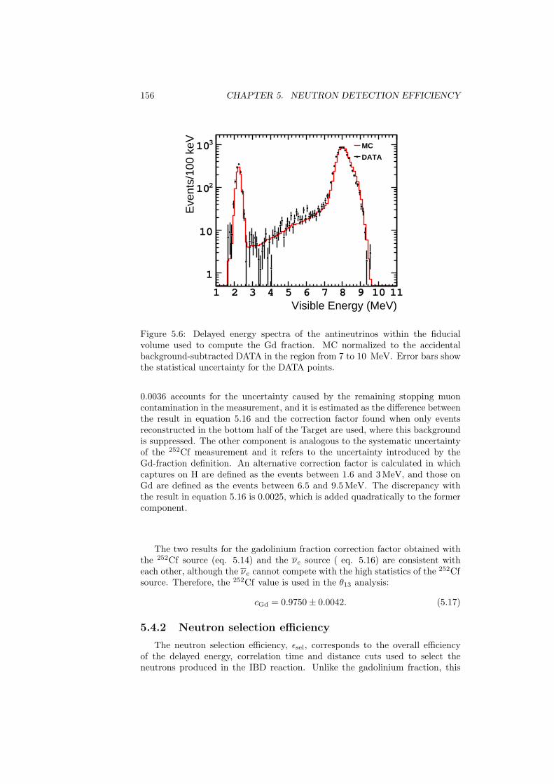
156 CHAPTER 5. NEUTRON DETECTION EFFICIENCY
Visible Energy (MeV)1 2 3 4 5 6 7 8 9 10 11
Eve
nts/
100
keV
1
10
210
310 MC
DATA
Figure 5.6: Delayed energy spectra of the antineutrinos within the fiducialvolume used to compute the Gd fraction. MC normalized to the accidentalbackground-subtracted DATA in the region from 7 to 10 MeV. Error bars showthe statistical uncertainty for the DATA points.
0.0036 accounts for the uncertainty caused by the remaining stopping muoncontamination in the measurement, and it is estimated as the difference betweenthe result in equation 5.16 and the correction factor found when only eventsreconstructed in the bottom half of the Target are used, where this backgroundis suppressed. The other component is analogous to the systematic uncertaintyof the 252Cf measurement and it refers to the uncertainty introduced by theGd-fraction definition. An alternative correction factor is calculated in whichcaptures on H are defined as the events between 1.6 and 3 MeV, and those onGd are defined as the events between 6.5 and 9.5 MeV. The discrepancy withthe result in equation 5.16 is 0.0025, which is added quadratically to the formercomponent.
The two results for the gadolinium fraction correction factor obtained withthe 252Cf source (eq. 5.14) and the νe source ( eq. 5.16) are consistent witheach other, although the νe cannot compete with the high statistics of the 252Cfsource. Therefore, the 252Cf value is used in the θ13 analysis:
cGd = 0.9750± 0.0042. (5.17)
5.4.2 Neutron selection efficiency
The neutron selection efficiency, εsel, corresponds to the overall efficiencyof the delayed energy, correlation time and distance cuts used to select theneutrons produced in the IBD reaction. Unlike the gadolinium fraction, this
5.4. NEUTRON DETECTION IN THE GADOLINIUM SELECTION 157
efficiency is not uniform within the detector and it will decrease as we approachto the borders of the Target affected by the change in the composition of thescintillator between Target and Gamma Catcher, which impacts the neutronsthermalization, and the higher probability that the released γ rays from theneutron captures are not fully absorbed in the scintillator volumes.
Thus, considering the cylindrical symmetry exhibited by the detector, theselection efficiency will be a function of two variables, εsel(z, ρ), where z is theheight and ρ =
√x2 + y2 is the radial distance to the center of the detector,
which is taken as the origin.Nevertheless, since the MC correction factor is applied to the global MC
νe normalization, regardless where the event happened, the local value of theefficiency εsel(z, ρ) has not practical interest, and what is truly relevant is theintegrated efficiency over the detector volume:
εsel =
∫V
εsel(z, ρ)dV
∫V
dV. (5.18)
Then, the neutron selection efficiency correction factor csel is written as the ratioof the volume-integrated selection efficiencies measured in the DATA and in theMC:
csel =εDATAsel
εMCsel
. (5.19)
Since the neutron selection efficiency consists of three selection cuts (de-layed energy, correlation time and correlation distance), one possibility is toevaluate all the cuts at the same time. This approach is known as inclusive.Another possibility is to assume that εsel can be factorized into the individualcut efficiencies:
εsel, exc = ε∆T · εEdelayed · ε∆R (5.20)
where ε∆T , εEdelayed , ε∆R are the correlation time, delayed energy and correlationdistance efficiencies, respectively. In this approach, called exclusive, only the cutgiving name to the efficiency is evaluated, while the others are kept fixed. Asusual, the specific definitions are source dependent and they can be found below.
5.4.2.1 Antineutrino measurement
The IBD events occur in all the detector, so the neutrons produced areespecially well-suited for a direct measurement of the volume-wide efficiency.
The inclusive neutron selection efficiency measured with the νe source isdefined as:
εsel, inc, IBD ≡N(0.5 < ∆T < 150µs ∩ 4 < Edelayed < 10 MeV ∩∆R < 1 m)
N(0.25 < ∆T < 200µs ∩ 3.5 < Edelayed < 10 MeV ∩∆R < 1.7 m),
(5.21)
where the numerator represents the number of IBD events passing the selectioncuts used in the gadolinium analysis (sec. 4.1.2), and the denominator corre-sponds to a larger number of events which satisfy a looser version of the cuts. Infigure 5.7, the inclusive neutron selection efficiency can be seen as a function of
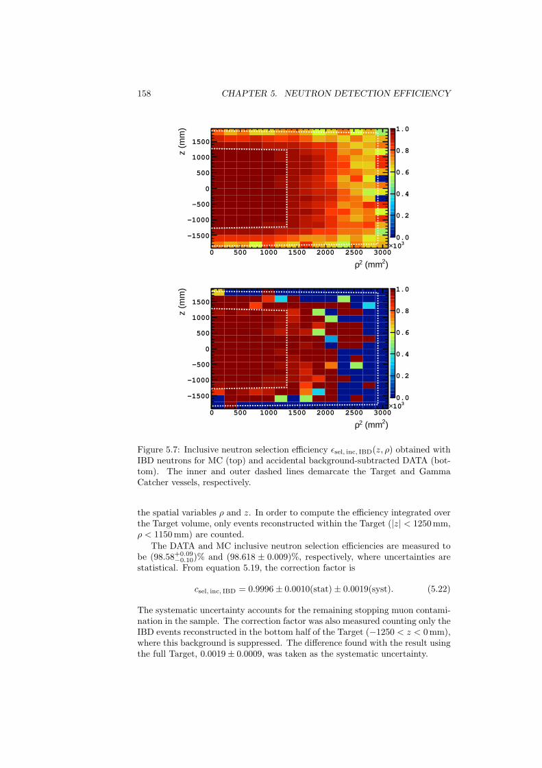
158 CHAPTER 5. NEUTRON DETECTION EFFICIENCY
)2 (mm2ρ0 500 1000 1500 2000 2500 3000
310×
z (m
m)
1500
1000
500
0
500
1000
1500
0.0
0.2
0.4
0.6
0.8
1.0
)2 (mm2ρ0 500 1000 1500 2000 2500 3000
310×
z (m
m)
1500
1000
500
0
500
1000
1500
0.0
0.2
0.4
0.6
0.8
1.0
Figure 5.7: Inclusive neutron selection efficiency εsel, inc, IBD(z, ρ) obtained withIBD neutrons for MC (top) and accidental background-subtracted DATA (bot-tom). The inner and outer dashed lines demarcate the Target and GammaCatcher vessels, respectively.
the spatial variables ρ and z. In order to compute the efficiency integrated overthe Target volume, only events reconstructed within the Target (|z| < 1250 mm,ρ < 1150 mm) are counted.
The DATA and MC inclusive neutron selection efficiencies are measured tobe (98.58+0.09
−0.10)% and (98.618 ± 0.009)%, respectively, where uncertainties arestatistical. From equation 5.19, the correction factor is
csel, inc, IBD = 0.9996± 0.0010(stat)± 0.0019(syst). (5.22)
The systematic uncertainty accounts for the remaining stopping muon contami-nation in the sample. The correction factor was also measured counting only theIBD events reconstructed in the bottom half of the Target (−1250 < z < 0 mm),where this background is suppressed. The difference found with the result usingthe full Target, 0.0019± 0.0009, was taken as the systematic uncertainty.
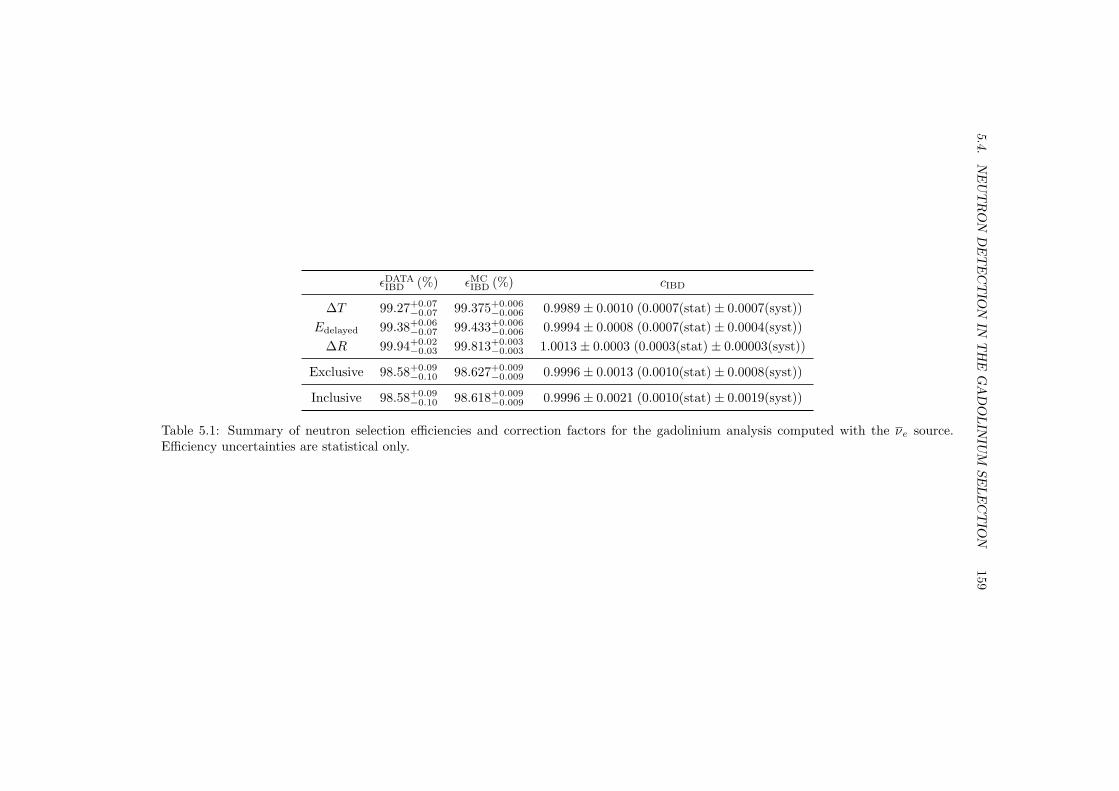
5.4.N
EU
TR
ON
DE
TE
CT
ION
INT
HE
GA
DO
LIN
IUM
SE
LE
CT
ION
159
εDATAIBD (%) εMC
IBD (%) cIBD
∆T 99.27+0.07−0.07 99.375+0.006
−0.006 0.9989± 0.0010 (0.0007(stat)± 0.0007(syst))Edelayed 99.38+0.06
−0.07 99.433+0.006−0.006 0.9994± 0.0008 (0.0007(stat)± 0.0004(syst))
∆R 99.94+0.02−0.03 99.813+0.003
−0.003 1.0013± 0.0003 (0.0003(stat)± 0.00003(syst))
Exclusive 98.58+0.09−0.10 98.627+0.009
−0.009 0.9996± 0.0013 (0.0010(stat)± 0.0008(syst))
Inclusive 98.58+0.09−0.10 98.618+0.009
−0.009 0.9996± 0.0021 (0.0010(stat)± 0.0019(syst))
Table 5.1: Summary of neutron selection efficiencies and correction factors for the gadolinium analysis computed with the νe source.Efficiency uncertainties are statistical only.
160 CHAPTER 5. NEUTRON DETECTION EFFICIENCY
An alternative correction factor can be computed following the exclusiveprescription. The correlation time, delayed energy and correlation distanceefficiencies are defined:
ε∆T, IBD ≡N(0.5 < ∆T < 150µs ∩ 4 < Edelayed < 10 MeV ∩∆R < 1 m)
N(0.25 < ∆T < 200µs ∩ 4 < Edelayed < 10 MeV ∩∆R < 1 m)(5.23)
εEdelayed, IBD ≡N(0.5 < ∆T < 150µs ∩ 4 < Edelayed < 10 MeV ∩∆R < 1 m)
N(0.5 < ∆T < 150µs ∩ 3.5 < Edelayed < 10 MeV ∩∆R < 1 m)(5.24)
ε∆R, IBD ≡N(0.5 < ∆T < 150µs ∩ 4 < Edelayed < 10 MeV ∩∆R < 1 m)
N(0.5 < ∆T < 150µs ∩ 4 < Edelayed < 10 MeV ∩∆R < 1.7 m).
(5.25)
The result of computing each efficiency for the DATA and MC, together with theindividual correction factor derived from their ratio can be found in table 5.1.The exclusive selection efficiencies, according to equation 5.20, are (98.58+0.09
−0.10)%for DATA and (98.627 ± 0.009)% for MC (uncertainties are statistical). Thecorrection factor is found to be
csel, exc, IBD = 0.9996± 0.0010(stat)± 0.0008(syst), (5.26)
where the systematic uncertainty has been computed as in the inclusive result(eq. 5.22). The smaller systematic uncertainty in the exclusive case compared tothe inclusive one is understood to come from the different denominators used inequation 5.21 and equations 5.23, 5.24, 5.25. Whereas for the inclusive efficiencyall the three cuts are relaxed simultaneously, thus increasing the probability ofbackground contamination; in the exclusive efficiency only one cut is loosenedat a time, so the background acceptance is smaller.
The fact that the two results in equations 5.22 and 5.26 agree nicely demon-strates that the background is under control, and that the hypothesized factor-ization of eq. 5.20 can be done. However, the inclusive correction is propagatedto the θ13 oscillation fit because the uncertainty is more conservative.
The impact of restricting the volume integration of equation 5.18 to theTarget was studied by varying the integral limits, as it is shown in figure 5.8.The evolution of the correction factor is consistent with a flat trend, establishingthat no bias was introduced because of the volume constraint.
Further investigations were performed to search for additional sources ofsystematic uncertainty. The efficiency definitions in equations 5.21, 5.23, 5.24,5.25 were perturbed by altering the denominators, either by tightening the cuts(the upper ∆T limit was moved to 175µs, the maximum ∆R was shortened to1.5 m, both separately and simultaneously) or by loosening even more the cuts(the lower Edelayed limit was moved to 3 MeV, the maximum ∆R was enlargedto 2 m, both separately and simultaneously). All resulted in non-significant dis-crepancies. The reproducibility of the method was tested by repeating the calcu-lation of the correction factors using an alternative MC simulation statistically-independent generated, finding exactly the same results. The influence of theGd concentration on the correction factors was examined by analyzing two MCsimulations produced with 960 mg/l and 1020 mg/l, which correspond to a ±3%variation in the standard value (989 mg/l). Both results were found to agreewithin statistical uncertainty with the ones obtained with the standard con-centration. Finally, the hypothesis that 9Li/8He and fast neutron events areinnocuous (since they have a neutron capture as delayed trigger) was put to the
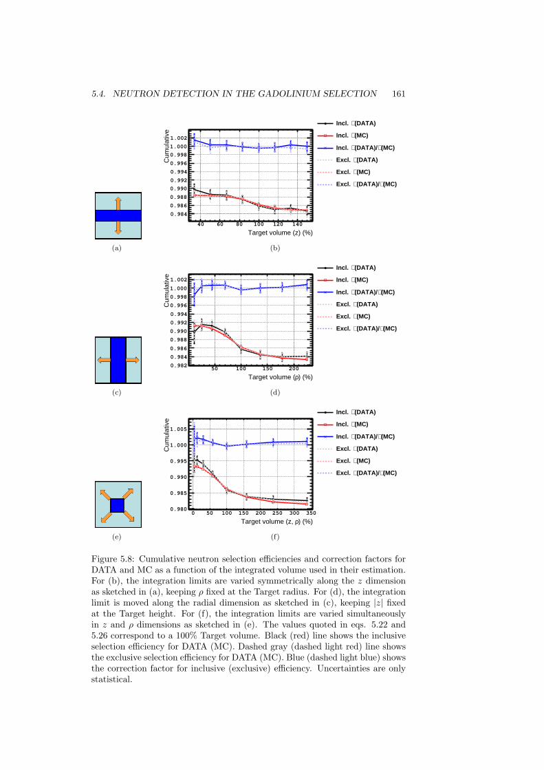
5.4. NEUTRON DETECTION IN THE GADOLINIUM SELECTION 161
(a)
Target volume (z) (%)40 60 80 100 120 140
Cum
ulat
ive
0.984
0.986
0.988
0.990
0.992
0.994
0.996
0.998
1.000
1.002
(DATA)∈Incl.
(MC)∈Incl.
(MC)∈(DATA)/∈Incl.
(DATA)∈Excl.
(MC)∈Excl.
(MC)∈(DATA)/∈Excl.
(b)
(c)
) (%)ρTarget volume (50 100 150 200
Cum
ulat
ive
0.982
0.984
0.986
0.988
0.990
0.992
0.994
0.996
0.998
1.000
1.002
(DATA)∈Incl.
(MC)∈Incl.
(MC)∈(DATA)/∈Incl.
(DATA)∈Excl.
(MC)∈Excl.
(MC)∈(DATA)/∈Excl.
(d)
(e)
) (%)ρTarget volume (z, 0 50 100 150 200 250 300 350
Cum
ulat
ive
0.980
0.985
0.990
0.995
1.000
1.005
(DATA)∈Incl.
(MC)∈Incl.
(MC)∈(DATA)/∈Incl.
(DATA)∈Excl.
(MC)∈Excl.
(MC)∈(DATA)/∈Excl.
(f)
Figure 5.8: Cumulative neutron selection efficiencies and correction factors forDATA and MC as a function of the integrated volume used in their estimation.For (b), the integration limits are varied symmetrically along the z dimensionas sketched in (a), keeping ρ fixed at the Target radius. For (d), the integrationlimit is moved along the radial dimension as sketched in (c), keeping |z| fixedat the Target height. For (f), the integration limits are varied simultaneouslyin z and ρ dimensions as sketched in (e). The values quoted in eqs. 5.22 and5.26 correspond to a 100% Target volume. Black (red) line shows the inclusiveselection efficiency for DATA (MC). Dashed gray (dashed light red) line showsthe exclusive selection efficiency for DATA (MC). Blue (dashed light blue) showsthe correction factor for inclusive (exclusive) efficiency. Uncertainties are onlystatistical.
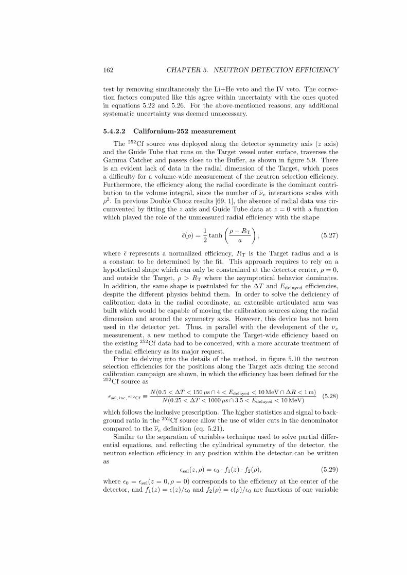
162 CHAPTER 5. NEUTRON DETECTION EFFICIENCY
test by removing simultaneously the Li+He veto and the IV veto. The correc-tion factors computed like this agree within uncertainty with the ones quotedin equations 5.22 and 5.26. For the above-mentioned reasons, any additionalsystematic uncertainty was deemed unnecessary.
5.4.2.2 Californium-252 measurement
The 252Cf source was deployed along the detector symmetry axis (z axis)and the Guide Tube that runs on the Target vessel outer surface, traverses theGamma Catcher and passes close to the Buffer, as shown in figure 5.9. Thereis an evident lack of data in the radial dimension of the Target, which posesa difficulty for a volume-wide measurement of the neutron selection efficiency.Furthermore, the efficiency along the radial coordinate is the dominant contri-bution to the volume integral, since the number of νe interactions scales withρ2. In previous Double Chooz results [69, 1], the absence of radial data was cir-cumvented by fitting the z axis and Guide Tube data at z = 0 with a functionwhich played the role of the unmeasured radial efficiency with the shape
ε(ρ) =12
tanh(ρ−RT
a
), (5.27)
where ε represents a normalized efficiency, RT is the Target radius and a isa constant to be determined by the fit. This approach requires to rely on ahypothetical shape which can only be constrained at the detector center, ρ = 0,and outside the Target, ρ > RT where the asymptotical behavior dominates.In addition, the same shape is postulated for the ∆T and Edelayed efficiencies,despite the different physics behind them. In order to solve the deficiency ofcalibration data in the radial coordinate, an extensible articulated arm wasbuilt which would be capable of moving the calibration sources along the radialdimension and around the symmetry axis. However, this device has not beenused in the detector yet. Thus, in parallel with the development of the νemeasurement, a new method to compute the Target-wide efficiency based onthe existing 252Cf data had to be conceived, with a more accurate treatment ofthe radial efficiency as its major request.
Prior to delving into the details of the method, in figure 5.10 the neutronselection efficiencies for the positions along the Target axis during the secondcalibration campaign are shown, in which the efficiency has been defined for the252Cf source as
εsel, inc, 252Cf ≡N(0.5 < ∆T < 150µs ∩ 4 < Edelayed < 10 MeV ∩∆R < 1 m)
N(0.25 < ∆T < 1000µs ∩ 3.5 < Edelayed < 10 MeV)(5.28)
which follows the inclusive prescription. The higher statistics and signal to back-ground ratio in the 252Cf source allow the use of wider cuts in the denominatorcompared to the νe definition (eq. 5.21).
Similar to the separation of variables technique used to solve partial differ-ential equations, and reflecting the cylindrical symmetry of the detector, theneutron selection efficiency in any position within the detector can be writtenas
εsel(z, ρ) = ε0 · f1(z) · f2(ρ), (5.29)
where ε0 = εsel(z = 0, ρ = 0) corresponds to the efficiency at the center of thedetector, and f1(z) = ε(z)/ε0 and f2(ρ) = ε(ρ)/ε0 are functions of one variable
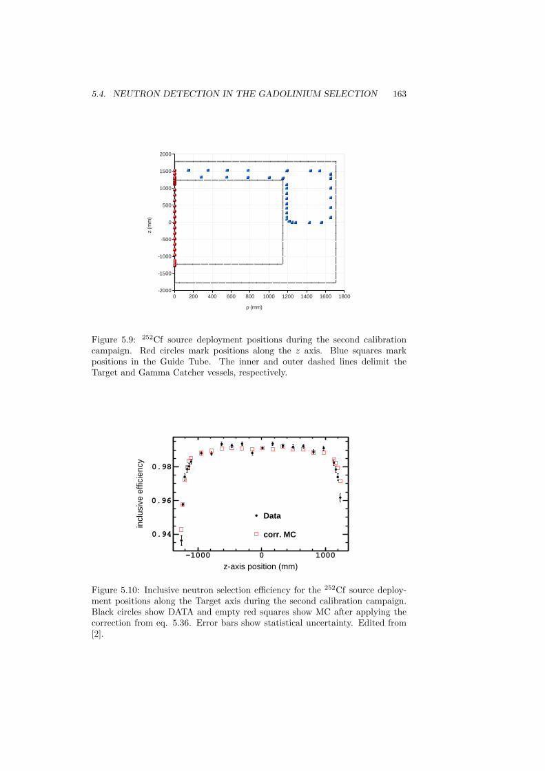
5.4. NEUTRON DETECTION IN THE GADOLINIUM SELECTION 163
0 200 400 600 800 1000 1200 1400 1600 1800-2000
-1500
-1000
-500
0
500
1000
1500
2000
ρ (mm)
z (m
m)
Figure 5.9: 252Cf source deployment positions during the second calibrationcampaign. Red circles mark positions along the z axis. Blue squares markpositions in the Guide Tube. The inner and outer dashed lines delimit theTarget and Gamma Catcher vessels, respectively.
z-axis position (mm)-1000 0 1000
incl
usiv
e ef
ficie
ncy
0.94
0.96
0.98
Data
corr. MC
Figure 5.10: Inclusive neutron selection efficiency for the 252Cf source deploy-ment positions along the Target axis during the second calibration campaign.Black circles show DATA and empty red squares show MC after applying thecorrection from eq. 5.36. Error bars show statistical uncertainty. Edited from[2].
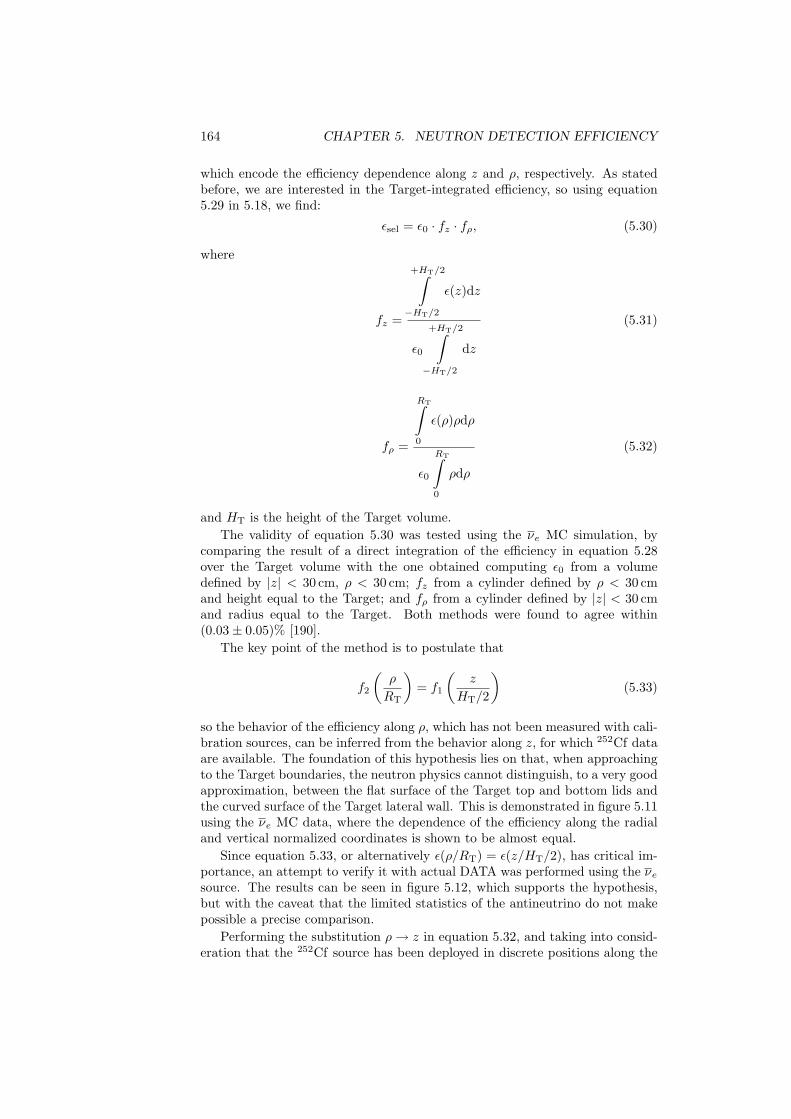
164 CHAPTER 5. NEUTRON DETECTION EFFICIENCY
which encode the efficiency dependence along z and ρ, respectively. As statedbefore, we are interested in the Target-integrated efficiency, so using equation5.29 in 5.18, we find:
εsel = ε0 · fz · fρ, (5.30)
where
fz =
+HT/2∫−HT/2
ε(z)dz
ε0
+HT/2∫−HT/2
dz
(5.31)
fρ =
RT∫0
ε(ρ)ρdρ
ε0
RT∫0
ρdρ
(5.32)
and HT is the height of the Target volume.The validity of equation 5.30 was tested using the νe MC simulation, by
comparing the result of a direct integration of the efficiency in equation 5.28over the Target volume with the one obtained computing ε0 from a volumedefined by |z| < 30 cm, ρ < 30 cm; fz from a cylinder defined by ρ < 30 cmand height equal to the Target; and fρ from a cylinder defined by |z| < 30 cmand radius equal to the Target. Both methods were found to agree within(0.03± 0.05)% [190].
The key point of the method is to postulate that
f2
(ρ
RT
)= f1
(z
HT/2
)(5.33)
so the behavior of the efficiency along ρ, which has not been measured with cali-bration sources, can be inferred from the behavior along z, for which 252Cf dataare available. The foundation of this hypothesis lies on that, when approachingto the Target boundaries, the neutron physics cannot distinguish, to a very goodapproximation, between the flat surface of the Target top and bottom lids andthe curved surface of the Target lateral wall. This is demonstrated in figure 5.11using the νe MC data, where the dependence of the efficiency along the radialand vertical normalized coordinates is shown to be almost equal.
Since equation 5.33, or alternatively ε(ρ/RT) = ε(z/HT/2), has critical im-portance, an attempt to verify it with actual DATA was performed using the νesource. The results can be seen in figure 5.12, which supports the hypothesis,but with the caveat that the limited statistics of the antineutrino do not makepossible a precise comparison.
Performing the substitution ρ→ z in equation 5.32, and taking into consid-eration that the 252Cf source has been deployed in discrete positions along the
5.4. NEUTRON DETECTION IN THE GADOLINIUM SELECTION 165
(a)
(b)
Figure 5.11: (a) f2(ρ/RT) (red) and f1(z/HT/2) (black) obtained from the νeMC simulation. (b) shows how the Target volume was divided into subvolumesalong z (top) and ρ (bottom) where the efficiency data points were calculated.The curves for positive and negative z values have been combined. (a) from[191], (b) from [190].
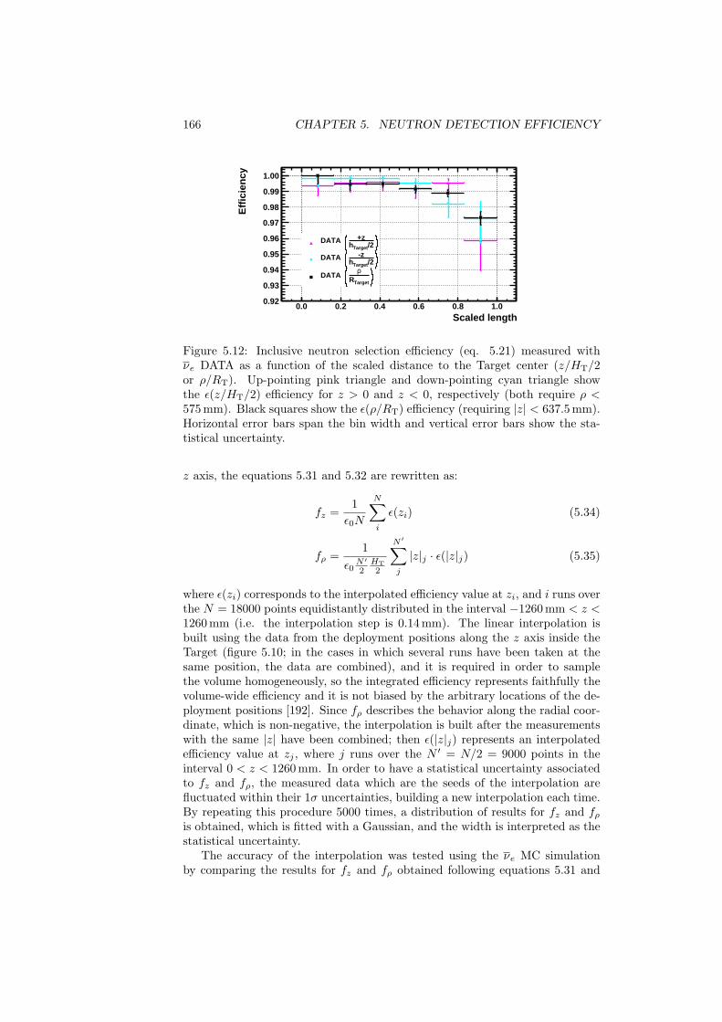
166 CHAPTER 5. NEUTRON DETECTION EFFICIENCY
Scaled length0.0 0.2 0.4 0.6 0.8 1.0
Eff
icie
ncy
0.92
0.93
0.94
0.95
0.96
0.97
0.98
0.99
1.00
/2Targeth+zDATA
/2Targeth-zDATA
TargetRρ
DATA
Figure 5.12: Inclusive neutron selection efficiency (eq. 5.21) measured withνe DATA as a function of the scaled distance to the Target center (z/HT/2or ρ/RT). Up-pointing pink triangle and down-pointing cyan triangle showthe ε(z/HT/2) efficiency for z > 0 and z < 0, respectively (both require ρ <575 mm). Black squares show the ε(ρ/RT) efficiency (requiring |z| < 637.5 mm).Horizontal error bars span the bin width and vertical error bars show the sta-tistical uncertainty.
z axis, the equations 5.31 and 5.32 are rewritten as:
fz =1ε0N
N∑i
ε(zi) (5.34)
fρ =1
ε0N ′
2HT2
N ′∑j
|z|j · ε(|z|j) (5.35)
where ε(zi) corresponds to the interpolated efficiency value at zi, and i runs overthe N = 18000 points equidistantly distributed in the interval −1260 mm < z <1260 mm (i.e. the interpolation step is 0.14 mm). The linear interpolation isbuilt using the data from the deployment positions along the z axis inside theTarget (figure 5.10; in the cases in which several runs have been taken at thesame position, the data are combined), and it is required in order to samplethe volume homogeneously, so the integrated efficiency represents faithfully thevolume-wide efficiency and it is not biased by the arbitrary locations of the de-ployment positions [192]. Since fρ describes the behavior along the radial coor-dinate, which is non-negative, the interpolation is built after the measurementswith the same |z| have been combined; then ε(|z|j) represents an interpolatedefficiency value at zj , where j runs over the N ′ = N/2 = 9000 points in theinterval 0 < z < 1260 mm. In order to have a statistical uncertainty associatedto fz and fρ, the measured data which are the seeds of the interpolation arefluctuated within their 1σ uncertainties, building a new interpolation each time.By repeating this procedure 5000 times, a distribution of results for fz and fρis obtained, which is fitted with a Gaussian, and the width is interpreted as thestatistical uncertainty.
The accuracy of the interpolation was tested using the νe MC simulationby comparing the results for fz and fρ obtained following equations 5.31 and
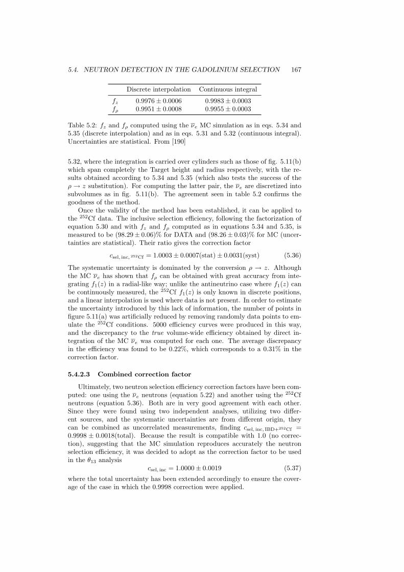
5.4. NEUTRON DETECTION IN THE GADOLINIUM SELECTION 167
Discrete interpolation Continuous integral
fz 0.9976± 0.0006 0.9983± 0.0003fρ 0.9951± 0.0008 0.9955± 0.0003
Table 5.2: fz and fρ computed using the νe MC simulation as in eqs. 5.34 and5.35 (discrete interpolation) and as in eqs. 5.31 and 5.32 (continuous integral).Uncertainties are statistical. From [190]
5.32, where the integration is carried over cylinders such as those of fig. 5.11(b)which span completely the Target height and radius respectively, with the re-sults obtained according to 5.34 and 5.35 (which also tests the success of theρ → z substitution). For computing the latter pair, the νe are discretized intosubvolumes as in fig. 5.11(b). The agreement seen in table 5.2 confirms thegoodness of the method.
Once the validity of the method has been established, it can be applied tothe 252Cf data. The inclusive selection efficiency, following the factorization ofequation 5.30 and with fz and fρ computed as in equations 5.34 and 5.35, ismeasured to be (98.29± 0.06)% for DATA and (98.26± 0.03)% for MC (uncer-tainties are statistical). Their ratio gives the correction factor
csel, inc, 252Cf = 1.0003± 0.0007(stat)± 0.0031(syst) (5.36)
The systematic uncertainty is dominated by the conversion ρ → z. Althoughthe MC νe has shown that fρ can be obtained with great accuracy from inte-grating f1(z) in a radial-like way; unlike the antineutrino case where f1(z) canbe continuously measured, the 252Cf f1(z) is only known in discrete positions,and a linear interpolation is used where data is not present. In order to estimatethe uncertainty introduced by this lack of information, the number of points infigure 5.11(a) was artificially reduced by removing randomly data points to em-ulate the 252Cf conditions. 5000 efficiency curves were produced in this way,and the discrepancy to the true volume-wide efficiency obtained by direct in-tegration of the MC νe was computed for each one. The average discrepancyin the efficiency was found to be 0.22%, which corresponds to a 0.31% in thecorrection factor.
5.4.2.3 Combined correction factor
Ultimately, two neutron selection efficiency correction factors have been com-puted: one using the νe neutrons (equation 5.22) and another using the 252Cfneutrons (equation 5.36). Both are in very good agreement with each other.Since they were found using two independent analyses, utilizing two differ-ent sources, and the systematic uncertainties are from different origin, theycan be combined as uncorrelated measurements, finding csel, inc, IBD+252Cf =0.9998 ± 0.0018(total). Because the result is compatible with 1.0 (no correc-tion), suggesting that the MC simulation reproduces accurately the neutronselection efficiency, it was decided to adopt as the correction factor to be usedin the θ13 analysis
csel, inc = 1.0000± 0.0019 (5.37)
where the total uncertainty has been extended accordingly to ensure the cover-age of the case in which the 0.9998 correction were applied.
168 CHAPTER 5. NEUTRON DETECTION EFFICIENCY
5.4.3 Spill-in/out
The Target scintillator acts as a natural fiducial volume in which the neu-trons from the IBD events are captured on Gd nuclei. However, some neutronscreated in the Target can escape into the Gamma Catcher and be captured on aH nucleus, which makes the event not to pass the Gd selection cuts, leading toa loss of expected νe. This is known as spill-out. On the other hand, IBD neu-trons created in the Gamma Catcher can enter into the Target and be capturedon a Gd nucleus, increasing the number of detected νe. This is called spill-in.Even though these two effects counterbalance, they do not cancel out. Becausethe Gamma Catcher surrounds the Target, the Gamma Catcher has a biggervolume capable of producing spill-in events. In addition, because the GammaCatcher scintillator is not loaded with Gd, the neutrons are able to travel alonger distance in it before they are captured. As a consequence, the numberof spill-in events surpasses the spill-out one, and there is a net spill-in current.
Unfortunately, the spill currents cannot be measured isolatedly in the DATA.The resolution of the position reconstruction does not allow to classify eventswith enough accuracy. Hence, the strategy of comparing the DATA to theMC simulation to compute a possible correction factor as it was done for theneutron selection efficiency cannot be followed, and the comparison betweendifferent MC simulations is left as the unique option.
The number of detected events (i.e. passing all selection cuts) in the simu-lation can be written as
Ndet = εdet(NT −NSO) +NSIdet +NSO
det (5.38)
where NT is the number of IBD interactions occurred in the Target, NSO isthe number of spill-out events, NSI
det is the number of spill-in events passingthe Gd selection, and NSO
det is the number of the IBD interactions in the Targetin which the neutron was captured outside on a 12C nucleus and pass the Gdselection anyway. εdet is the detection efficiency of the neutrons produced andcaptured within the Target, and it is defined as the product of the Gd fractionand the selection efficiency in the Geant4 simulation, which are corrected usingthe factors computed in the previous sections to match the DATA.
Equation 5.38 can be rewritten as
Ndet = εdet ·NT(1 + φspilldet ) (5.39)
which shows explicitly how the number of detected IBD events in the Target,εdet ·NT, receives a correction from the detected fractional spill current:
φspilldet ≡
1NT
(NSI
det +NSOdet
εdet−NSO
)(5.40)
The (1 + φspilldet ) correction can be identified with the neutron mobility factor,
kspill, in equation 5.6.Because the spill current is related to the neutron transport, it is very sen-
sitive to the low energy neutron physics. As it has been described in section5.2, in this energy regime it is particularly relevant how the molecular bondsof H are simulated. The default MC simulation in Double Chooz uses Geant4,which is optimized for high-energy neutrons, together with a patch, NeutronTH,
5.4. NEUTRON DETECTION IN THE GADOLINIUM SELECTION 169
for kinetic energies below 4 eV. This MC is compared against Tripoli4 [193],a code specifically designed for the simulation of the low energy neutron trans-port (originally for reactor physics). Whereas NeutronTH uses an analyticalcorrection to simulate the effect of the hydrogen bonds, Tripoli4 uses exclu-sively experimental data. The hydrogen nuclei are considered to be bound inCH2 groups, which is the dominant structure in dodecane, the main compo-nent of the scintillator. Including other bonds, such as aromatic rings, doesnot introduce a significant discrepancy. Tripoli4 uses the same detector ge-ometry as Geant4, but the generation of γ rays from radiative captures is notactivated since it lacks a model for the scintillator light emission, propagationand collection in the PMTs (which makes unavailable all the variables derivedfrom the event reconstruction). In order to simulate the detection process, theevents are weighted according to probabilities of detection built from the Geant4simulation using the event location.
The detected fractional spill current (eq. 5.40) is found to be 2.08% using theGeant4-NeutronTH simulation, and 2.36% using the Tripoli4 simulation. SinceNeutronTH describes the neutron thermalization sufficiently well, no correctionfactor was considered necessary
cspill = 1.0000± 0.0027, (5.41)
and the difference between the two simulations was taken as the normalizationuncertainty induced by the spill effect.
5.4.4 Summary
In table 5.3 all the individual efficiency corrections and uncertainties thatintervene in the computation of the total MC normalization correction factor forthe Gd selection are summarized. Those which are not related to the neutronphysics have been described in chapter 4 (see table 4.1). This section has beendevoted to describe the computation of the corrections related to the neutrondetection efficiency (Gd fraction, neutron selection efficiency and spill-in/out).This thorough treatment is justified since the neutron detection efficiency isthe dominant source of uncertainty in the normalization of the expected νe,totaling 0.54%. Nevertheless, compared to the previous Double Chooz result[1], in which this uncertainty added up to 0.96%, the improvement brought bythe new methods described here is evident.
Furthermore, the new result paves the way for the two-detector phase, whenonly the uncorrelated uncertainties between detectors will affect the precisionof the sin2(2θ13) measurement. Since the two Target volumes are filled with thesame scintillator, which was produced as a single batch, the portion of uncorre-lated uncertainty in the Gd fraction will be simply the statistical uncertainty,which currently is 0.11% and it can be reduced even further by acquiring more252Cf calibration data at the center of the detectors. In addition, because thetwo detectors have been made identical, the uncertainty caused by the spillcurrent will cancel almost completely, up to an uncorrelated residual causedby the different acceptance of the two detectors to the νe flux. Hence, themajor contribution to the uncertainty will be the neutron selection efficiency,which currently amounts to 0.19%. This uncertainty is composed of a statisti-cal component, which is inherently uncorrelated, which will be reduced as more
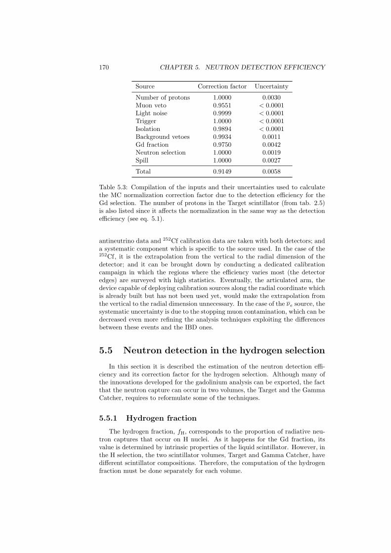
170 CHAPTER 5. NEUTRON DETECTION EFFICIENCY
Source Correction factor Uncertainty
Number of protons 1.0000 0.0030Muon veto 0.9551 < 0.0001Light noise 0.9999 < 0.0001Trigger 1.0000 < 0.0001Isolation 0.9894 < 0.0001Background vetoes 0.9934 0.0011Gd fraction 0.9750 0.0042Neutron selection 1.0000 0.0019Spill 1.0000 0.0027
Total 0.9149 0.0058
Table 5.3: Compilation of the inputs and their uncertainties used to calculatethe MC normalization correction factor due to the detection efficiency for theGd selection. The number of protons in the Target scintillator (from tab. 2.5)is also listed since it affects the normalization in the same way as the detectionefficiency (see eq. 5.1).
antineutrino data and 252Cf calibration data are taken with both detectors; anda systematic component which is specific to the source used. In the case of the252Cf, it is the extrapolation from the vertical to the radial dimension of thedetector; and it can be brought down by conducting a dedicated calibrationcampaign in which the regions where the efficiency varies most (the detectoredges) are surveyed with high statistics. Eventually, the articulated arm, thedevice capable of deploying calibration sources along the radial coordinate whichis already built but has not been used yet, would make the extrapolation fromthe vertical to the radial dimension unnecessary. In the case of the νe source, thesystematic uncertainty is due to the stopping muon contamination, which can bedecreased even more refining the analysis techniques exploiting the differencesbetween these events and the IBD ones.
5.5 Neutron detection in the hydrogen selection
In this section it is described the estimation of the neutron detection effi-ciency and its correction factor for the hydrogen selection. Although many ofthe innovations developed for the gadolinium analysis can be exported, the factthat the neutron capture can occur in two volumes, the Target and the GammaCatcher, requires to reformulate some of the techniques.
5.5.1 Hydrogen fraction
The hydrogen fraction, fH, corresponds to the proportion of radiative neu-tron captures that occur on H nuclei. As it happens for the Gd fraction, itsvalue is determined by intrinsic properties of the liquid scintillator. However, inthe H selection, the two scintillator volumes, Target and Gamma Catcher, havedifferent scintillator compositions. Therefore, the computation of the hydrogenfraction must be done separately for each volume.
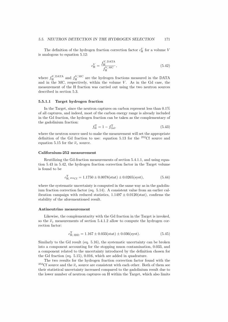
5.5. NEUTRON DETECTION IN THE HYDROGEN SELECTION 171
The definition of the hydrogen fraction correction factor cVH for a volume Vis analogous to equation 5.12:
cVH =fV,DATA
H
fV,MCH
, (5.42)
where fV,DATAH and fV,MC
H are the hydrogen fractions measured in the DATAand in the MC, respectively, within the volume V . As in the Gd case, themeasurement of the H fraction was carried out using the two neutron sourcesdescribed in section 5.3.
5.5.1.1 Target hydrogen fraction
In the Target, since the neutron captures on carbon represent less than 0.1%of all captures, and indeed, most of the carbon energy range is already includedin the Gd fraction, the hydrogen fraction can be taken as the complementary ofthe gadolinium fraction:
fTH = 1− fT
Gd, (5.43)
where the neutron source used to make the measurement will set the appropriatedefinition of the Gd fraction to use: equation 5.13 for the 252Cf source andequation 5.15 for the νe source.
Californium-252 measurement
Reutilizing the Gd-fraction measurements of section 5.4.1.1, and using equa-tion 5.43 in 5.42, the hydrogen fraction correction factor in the Target volumeis found to be
cTH, 252Cf = 1.1750± 0.0078(stat)± 0.0265(syst), (5.44)
where the systematic uncertainty is computed in the same way as in the gadolin-ium fraction correction factor (eq. 5.14). A consistent value from an earlier cal-ibration campaign with reduced statistics, 1.1497 ± 0.0120(stat), confirms thestability of the aforementioned result.
Antineutrino measurement
Likewise, the complementarity with the Gd fraction in the Target is invoked,so the νe measurements of section 5.4.1.2 allow to compute the hydrogen cor-rection factor:
cTH, IBD = 1.167± 0.033(stat)± 0.036(syst). (5.45)
Similarly to the Gd result (eq. 5.16), the systematic uncertainty can be brokeninto a component accounting for the stopping muon contamination, 0.033, anda component related to the uncertainty introduced by the definition chosen forthe Gd fraction (eq. 5.15), 0.016, which are added in quadrature.
The two results for the hydrogen fraction correction factor found with the252Cf source and the νe source are consistent with each other. Both of them seetheir statistical uncertainty increased compared to the gadolinium result due tothe lower number of neutron captures on H within the Target, which also limits
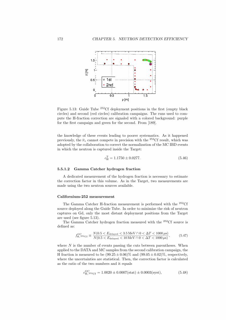
172 CHAPTER 5. NEUTRON DETECTION EFFICIENCY
Figure 5.13: Guide Tube 252Cf deployment positions in the first (empty blackcircles) and second (red circles) calibration campaigns. The runs used to com-pute the H-fraction correction are signaled with a colored background: purplefor the first campaign and green for the second. From [189].
the knowledge of these events leading to poorer systematics. As it happenedpreviously, the νe cannot compete in precision with the 252Cf result, which wasadopted by the collaboration to correct the normalization of the MC IBD eventsin which the neutron is captured inside the Target:
cTH = 1.1750± 0.0277. (5.46)
5.5.1.2 Gamma Catcher hydrogen fraction
A dedicated measurement of the hydrogen fraction is necessary to estimatethe correction factor in this volume. As in the Target, two measurements aremade using the two neutron sources available.
Californium-252 measurement
The Gamma Catcher H-fraction measurement is performed with the 252Cfsource deployed along the Guide Tube. In order to minimize the risk of neutroncaptures on Gd, only the most distant deployment positions from the Targetare used (see figure 5.13).
The Gamma Catcher hydrogen fraction measured with the 252Cf source isdefined as:
fGCH, 252Cf ≡
N(0.5 < Edelayed < 3.5 MeV ∩ 0 < ∆T < 1000µs)
N(0.5 < Edelayed < 10 MeV ∩ 0 < ∆T < 1000µs), (5.47)
where N is the number of events passing the cuts between parentheses. Whenapplied to the DATA and MC samples from the second calibration campaign, theH fraction is measured to be (99.25± 0.06)% and (99.05± 0.02)%, respectively,where the uncertainties are statistical. Then, the correction factor is calculatedas the ratio of the two numbers and it equals
cGCH, 252Cf = 1.0020± 0.0007(stat)± 0.0003(syst), (5.48)
5.5. NEUTRON DETECTION IN THE HYDROGEN SELECTION 173
visible energy (MeV)0 5 10 15 20
even
ts /
0.2
MeV
-710
-610
-510
-410
-310
-210
-110
1DATA
MC
Figure 5.14: Delayed energy spectra of the second calibration campaign 252Cfruns in the Guide Tube (see fig. 5.13) used to compute the Gamma Catcherhydrogen fraction. The MC (red histogram) has been normalized to the DATA(black points) integral. Error bars show the DATA statistical uncertainty. From[194].
where the systematic uncertainty corresponds to the uncertainty due to theparticular definition chosen. It is estimated as the difference in the correctionfactor found when the delayed energy lower limit is moved from 0.5 MeV to1.5 MeV, to account for the discrepancy between DATA and MC observed atlow energies in the Target. However, in the Gamma Catcher the DATA andMC spectra exhibit good agreement in all the energy range (see figure 5.14),resulting in a much smaller uncertainty.
The stability of the result was examined by computing cGCH, 252Cf using the
data from the first calibration campaign, which happens to have more run timein that part of the detector (160 min vs. 65 min). The value found, 1.0023 ±0.0005(stat), is in excellent agreement with the one in equation 5.48.
Antineutrino measurement
In order to compute the Gamma Catcher hydrogen fraction, in which allthe possible delayed energies resulting from neutron captures in the scintilla-tor must be considered, the ANN cut cannot be used since it is not designedto work beyond a delayed energy of 3.5 MeV, so an extra cut on the promptenergy Eprompt > 4 MeV is used to suppress the accidental contamination. Fur-thermore, the FV Gd cut, Edelayed > 0.068 · exp(FV/1.23), is added to the Hcut to extend the stopping muon and light noise rejection up to high energies.Analogous to the fiducial volume defined to measure the Gd fraction in section5.4.1.2, to maximize the probability of selecting candidates that have occurredwithin the Gamma Catcher; both the prompt and the delayed vertices are re-quired to be reconstructed inside it, i.e. |z| < 1837.24 mm and ρ < 1708 mm,but out of the Target (which occupies the volume given by |z| < 1274.54 mm
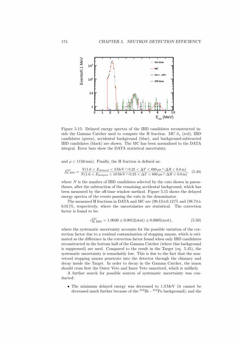
174 CHAPTER 5. NEUTRON DETECTION EFFICIENCY
(MeV)vis E0 1 2 3 4 5 6 7 8 9 10
Eve
nts/
0.1
MeV
1
10
210
310On-time
MC
On t - off t
Off-time
Figure 5.15: Delayed energy spectra of the IBD candidates reconstructed in-side the Gamma Catcher used to compute the H fraction. MC νe (red), IBDcandidates (green), accidental background (blue), and background-subtractedIBD candidates (black) are shown. The MC has been normalized to the DATAintegral. Error bars show the DATA statistical uncertainty.
and ρ < 1150 mm). Finally, the H fraction is defined as:
fGCH, IBD =
N(1.6 < Edelayed < 3 MeV ∩ 0.25 < ∆T < 600µs ∩∆R < 0.8 m)
N(1.6 < Edelayed < 10 MeV ∩ 0.25 < ∆T < 600µs ∩∆R < 0.8 m), (5.49)
where N is the number of IBD candidates selected by the cuts shown in paren-theses, after the subtraction of the remaining accidental background, which hasbeen measured by the off-time window method. Figure 5.15 shows the delayedenergy spectra of the events passing the cuts in the denominator.
The measured H fractions in DATA and MC are (99.13±0.12)% and (98.74±0.01)%, respectively, where the uncertainties are statistical. The correctionfactor is found to be:
cGCH, IBD = 1.0040± 0.0012(stat)± 0.0005(syst), (5.50)
where the systematic uncertainty accounts for the possible variation of the cor-rection factor due to a residual contamination of stopping muons, which is esti-mated as the difference in the correction factor found when only IBD candidatesreconstructed in the bottom half of the Gamma Catcher (where this backgroundis suppressed) are used. Compared to the result in the Target (eq. 5.45), thesystematic uncertainty is remarkably low. This is due to the fact that the non-vetoed stopping muons penetrate into the detector through the chimney anddecay inside the Target. In order to decay in the Gamma Catcher, the muonshould cross first the Outer Veto and Inner Veto unnoticed, which is unlikely.
A further search for possible sources of systematic uncertainty was con-ducted:
• The minimum delayed energy was decreased to 1.3 MeV (it cannot bedecreased much further because of the 212Bi−212Po background); and the
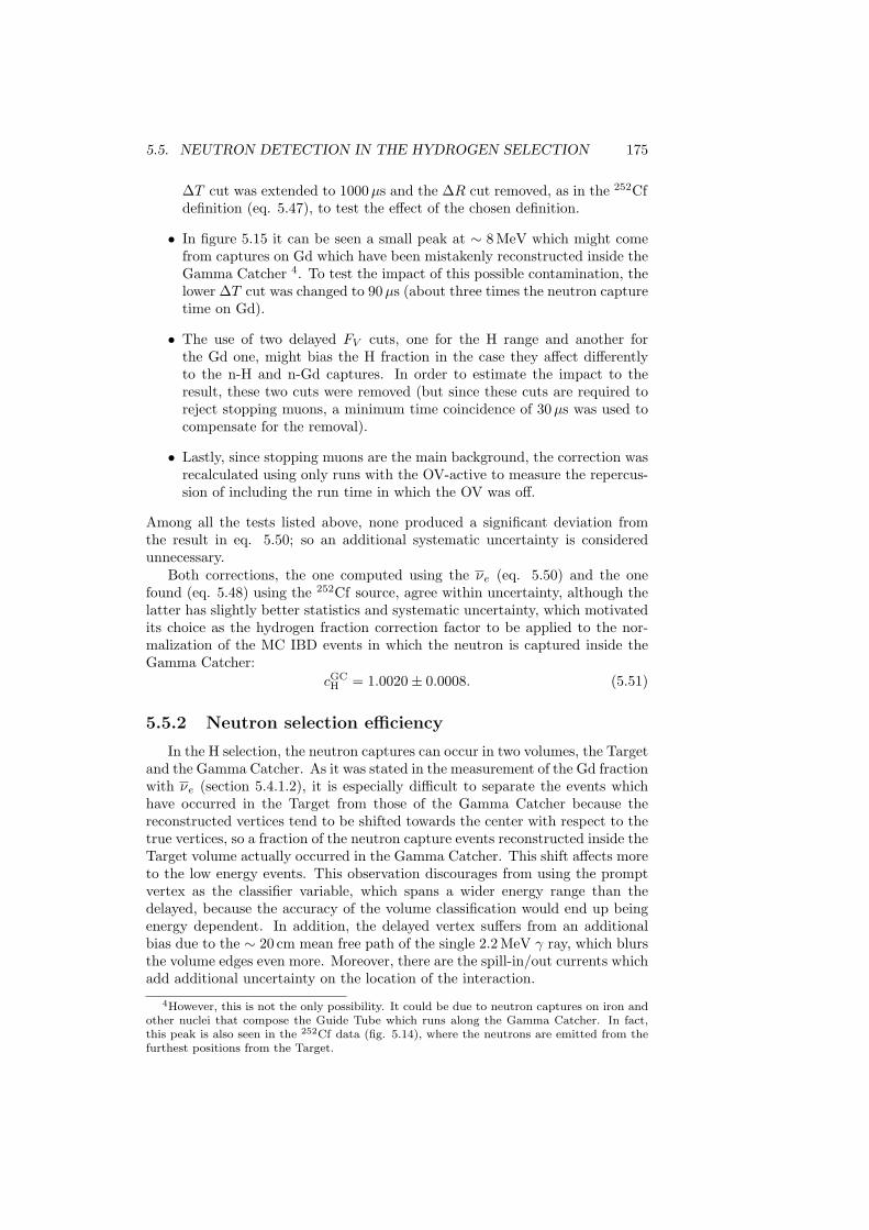
5.5. NEUTRON DETECTION IN THE HYDROGEN SELECTION 175
∆T cut was extended to 1000µs and the ∆R cut removed, as in the 252Cfdefinition (eq. 5.47), to test the effect of the chosen definition.
• In figure 5.15 it can be seen a small peak at ∼ 8 MeV which might comefrom captures on Gd which have been mistakenly reconstructed inside theGamma Catcher 4. To test the impact of this possible contamination, thelower ∆T cut was changed to 90µs (about three times the neutron capturetime on Gd).
• The use of two delayed FV cuts, one for the H range and another forthe Gd one, might bias the H fraction in the case they affect differentlyto the n-H and n-Gd captures. In order to estimate the impact to theresult, these two cuts were removed (but since these cuts are required toreject stopping muons, a minimum time coincidence of 30µs was used tocompensate for the removal).
• Lastly, since stopping muons are the main background, the correction wasrecalculated using only runs with the OV-active to measure the repercus-sion of including the run time in which the OV was off.
Among all the tests listed above, none produced a significant deviation fromthe result in eq. 5.50; so an additional systematic uncertainty is consideredunnecessary.
Both corrections, the one computed using the νe (eq. 5.50) and the onefound (eq. 5.48) using the 252Cf source, agree within uncertainty, although thelatter has slightly better statistics and systematic uncertainty, which motivatedits choice as the hydrogen fraction correction factor to be applied to the nor-malization of the MC IBD events in which the neutron is captured inside theGamma Catcher:
cGCH = 1.0020± 0.0008. (5.51)
5.5.2 Neutron selection efficiency
In the H selection, the neutron captures can occur in two volumes, the Targetand the Gamma Catcher. As it was stated in the measurement of the Gd fractionwith νe (section 5.4.1.2), it is especially difficult to separate the events whichhave occurred in the Target from those of the Gamma Catcher because thereconstructed vertices tend to be shifted towards the center with respect to thetrue vertices, so a fraction of the neutron capture events reconstructed inside theTarget volume actually occurred in the Gamma Catcher. This shift affects moreto the low energy events. This observation discourages from using the promptvertex as the classifier variable, which spans a wider energy range than thedelayed, because the accuracy of the volume classification would end up beingenergy dependent. In addition, the delayed vertex suffers from an additionalbias due to the ∼ 20 cm mean free path of the single 2.2 MeV γ ray, which blursthe volume edges even more. Moreover, there are the spill-in/out currents whichadd additional uncertainty on the location of the interaction.
4However, this is not the only possibility. It could be due to neutron captures on iron andother nuclei that compose the Guide Tube which runs along the Gamma Catcher. In fact,this peak is also seen in the 252Cf data (fig. 5.14), where the neutrons are emitted from thefurthest positions from the Target.
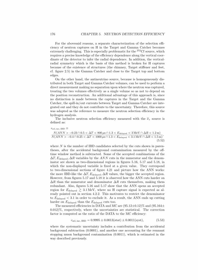
176 CHAPTER 5. NEUTRON DETECTION EFFICIENCY
For the abovesaid reasons, a separate characterization of the selection effi-ciency of neutron captures on H in the Target and Gamma Catcher becomesextremely challenging. This is especially problematic for the 252Cf source, whichrequires a precise knowledge of the efficiency dependence along the vertical coor-dinate of the detector to infer the radial dependence. In addition, the vertical-radial symmetry which is the basis of this method is broken for H capturesbecause of the existence of structures (the chimney, Target stiffener and feet,cf. figure 2.5) in the Gamma Catcher and close to the Target top and bottomedges.
On the other hand, the antineutrino source, because is homogeneously dis-tributed in both Target and Gamma Catcher volumes, can be used to perform adirect measurement making no separation upon where the neutron was captured,treating the two volumes effectively as a single volume so as not to depend onthe position reconstruction. An additional advantage of this approach is, sinceno distinction is made between the captures in the Target and the GammaCatcher, the spill-in/out currents between Target and Gamma Catcher are inte-grated out and they do not contribute to the uncertainty. Therefore, this sourcewas adopted as the reference to measure the neutron selection efficiency in thehydrogen analysis.
The inclusive neutron selection efficiency measured with the νe source isdefined as:
εsel, inc, IBD ≡N(ANN > −0.23 ∩ 0.5 < ∆T < 800µs ∩ 1.3 < Edelayed < 3 MeV ∩∆R < 1.2 m)
N(ANN > −0.4 ∩ 0.25 < ∆T < 1000µs ∩ 1.3 < Edelayed < 3.1 MeV ∩∆R < 1.5 m),
(5.52)
where N is the number of IBD candidates selected by the cuts shown in paren-theses, after the accidental background contamination measured by the off-time window method is subtracted. Some of the accepted combinations of the∆T,Edelayed,∆R variables by the ANN cuts in the numerator and the denom-inator are shown as two-dimensional regions in figures 5.16, 5.17 and 5.18, inwhich the non-displayed variable is fixed at a given value. They correspondto two-dimensional sections of figure 4.21 and picture how the ANN works:the more IBD-like the ∆T,Edelayed,∆R values, the bigger the accepted region.However, from figures 5.17 and 5.18 it is observed how the ANN cuts harder on∆R than the numerator and denominator ∆R cuts themselves, making themredundant. Also, figures 5.16 and 5.17 show that the ANN opens an acceptedregion for Edelayed & 3.1 MeV, where no H capture signal is expected as al-ready pointed out in section 4.2.2. This motivates to restrict the denominatorto Edelayed < 3.1 in order to exclude it. As a result, the ANN ends up cuttingharder on Edelayed than the Edelayed cuts too.
The measured efficiencies in DATA and MC are (95.12±0.12)% and (95.164±0.012)%, respectively, where the uncertainties are statistical. The correctionfactor is computed as the ratio of the DATA to the MC efficiency:
csel, inc, IBD = 0.9995± 0.0013(stat)± 0.0011(syst), (5.53)
where the systematic uncertainty includes a contribution from the accidentalbackground subtraction (0.0001), and another one accounting for the remnantstopping muon background contamination (0.0011), which is estimated in theway described previously.
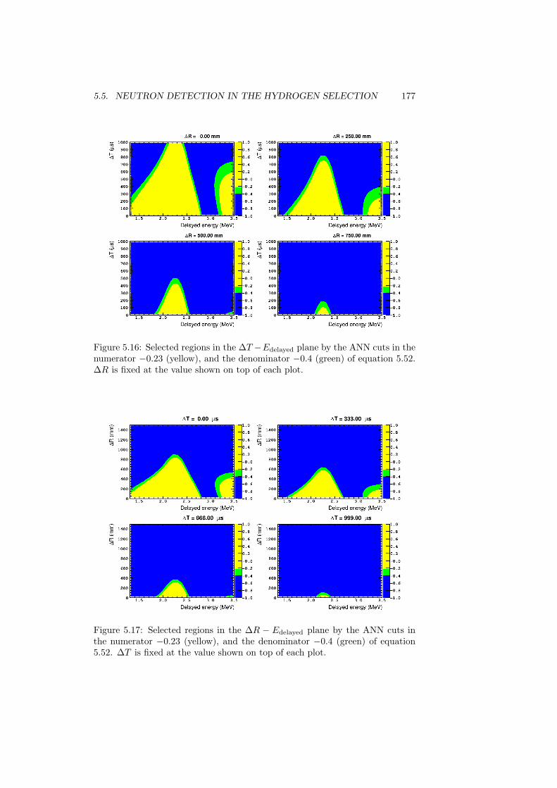
5.5. NEUTRON DETECTION IN THE HYDROGEN SELECTION 177
Figure 5.16: Selected regions in the ∆T −Edelayed plane by the ANN cuts in thenumerator −0.23 (yellow), and the denominator −0.4 (green) of equation 5.52.∆R is fixed at the value shown on top of each plot.
Figure 5.17: Selected regions in the ∆R − Edelayed plane by the ANN cuts inthe numerator −0.23 (yellow), and the denominator −0.4 (green) of equation5.52. ∆T is fixed at the value shown on top of each plot.
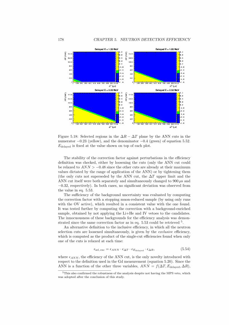
178 CHAPTER 5. NEUTRON DETECTION EFFICIENCY
Figure 5.18: Selected regions in the ∆R − ∆T plane by the ANN cuts in thenumerator −0.23 (yellow), and the denominator −0.4 (green) of equation 5.52.Edelayed is fixed at the value shown on top of each plot.
The stability of the correction factor against perturbations in the efficiencydefinition was checked, either by loosening the cuts (only the ANN cut couldbe relaxed to ANN > −0.48 since the other cuts are already at their maximumvalues dictated by the range of application of the ANN) or by tightening them(the only cuts not superseded by the ANN cut, the ∆T upper limit and theANN cut itself were both separately and simultaneously changed to 900µs and−0.32, respectively). In both cases, no significant deviation was observed fromthe value in eq. 5.53.
The sufficiency of the background uncertainty was evaluated by computingthe correction factor with a stopping muon-reduced sample (by using only runswith the OV active), which resulted in a consistent value with the one found.It was tested further by computing the correction with a background-enrichedsample, obtained by not applying the Li+He and IV vetoes to the candidates.The innocuousness of these backgrounds for the efficiency analysis was demon-strated since the same correction factor as in eq. 5.53 could be retrieved 5.
An alternative definition to the inclusive efficiency, in which all the neutronselection cuts are loosened simultaneously, is given by the exclusive efficiency,which is computed as the product of the single-cut efficiencies found when onlyone of the cuts is relaxed at each time:
εsel, exc = εANN · ε∆T · εEdelayed · ε∆R, (5.54)
where εANN , the efficiency of the ANN cut, is the only novelty introduced withrespect to the definition used in the Gd measurement (equation 5.20). Since theANN is a function of the other three variables, ANN = f(∆T,Edelayed,∆R),
5This also confirmed the robustness of the analysis despite not having the MPS veto, whichwas adopted after the conclusion of this study.
5.5. NEUTRON DETECTION IN THE HYDROGEN SELECTION 179
the factorization in equation 5.54 fails to isolate the effect of each cut, for whichreason it is only considered as a cross-check to the inclusive value.
For the H analysis, the single-cut efficiencies are defined as:
εANN, IBD ≡N(ANN > −0.23 ∩ 0.5 < ∆T < 800µs ∩ 1.3 < Edelayed < 3 MeV ∩∆R < 1.2 m)
N(ANN > −0.4 ∩ 0.5 < ∆T < 800µs ∩ 1.3 < Edelayed < 3 MeV ∩∆R < 1.2 m)(5.55)
ε∆T, IBD ≡N(ANN > −0.23 ∩ 0.5 < ∆T < 800µs ∩ 1.3 < Edelayed < 3 MeV ∩∆R < 1.2 m)
N(ANN > −0.23 ∩ 0.25 < ∆T < 1000µs ∩ 1.3 < Edelayed < 3 MeV ∩∆R < 1.2 m)(5.56)
εEdelayed, IBD ≡ 1 (5.57)
ε∆R, IBD ≡ 1 (5.58)
where εEdelayed, IBD ≡ 1 and ε∆R, IBD ≡ 1 because these cuts are superseded bythe ANN cut as explained before. The results of each single-cut efficiency forthe DATA and MC and the individual correction factor derived from their ratioare summarized in table 5.4.
The final exclusive selection efficiencies, from equation 5.54, are (95.22+0.12−0.13)%
for DATA and (95.241±0.012)% for MC (uncertainties are statistical). The cor-rection factor is found to be
csel, exc, IBD = 0.9997± 0.0013(stat)± 0.0009(syst), (5.59)
where the systematic uncertainty has the same contributions as the inclusiveresult (eq. 5.53), with which shows a very good agreement.
As long as the correction factor found is consistent with 1.0, that is, the MCsimulation reproduces faithfully the neutron selection efficiency as it is measuredin the DATA, the final neutron selection efficiency correction factor which willbe used in the θ13 analysis can be taken as:
csel, inc = 1.0000± 0.0022, (5.60)
where the uncertainty has been modified to ensure at least the same coverageas in the original result in equation 5.53.
5.5.3 Spill
When the signal is given by the neutron captures on hydrogen, the spillphenomenon becomes more complex than in the gadolinium capture case. Nowthe neutron can travel from the Target to the Gamma Catcher (and vice versa)and still produce a detectable signal since there are H nuclei in both scintillators,so the spill-in and spill-out cases of the Gd lose their meaning. Moreover,the neutron can also be captured on the H nuclei which make up the acrylicvessels. Finally, even though the Buffer is filled with non-scintillating mineraloil, an event produced outside the Gamma Catcher but close enough to it canbe detected if part of its energy is deposited in the scintillator.
In a general way, the number of detected νe events can be written as
Ndet = NTdet + Φint
det +NGCdet + Φext
det, (5.61)
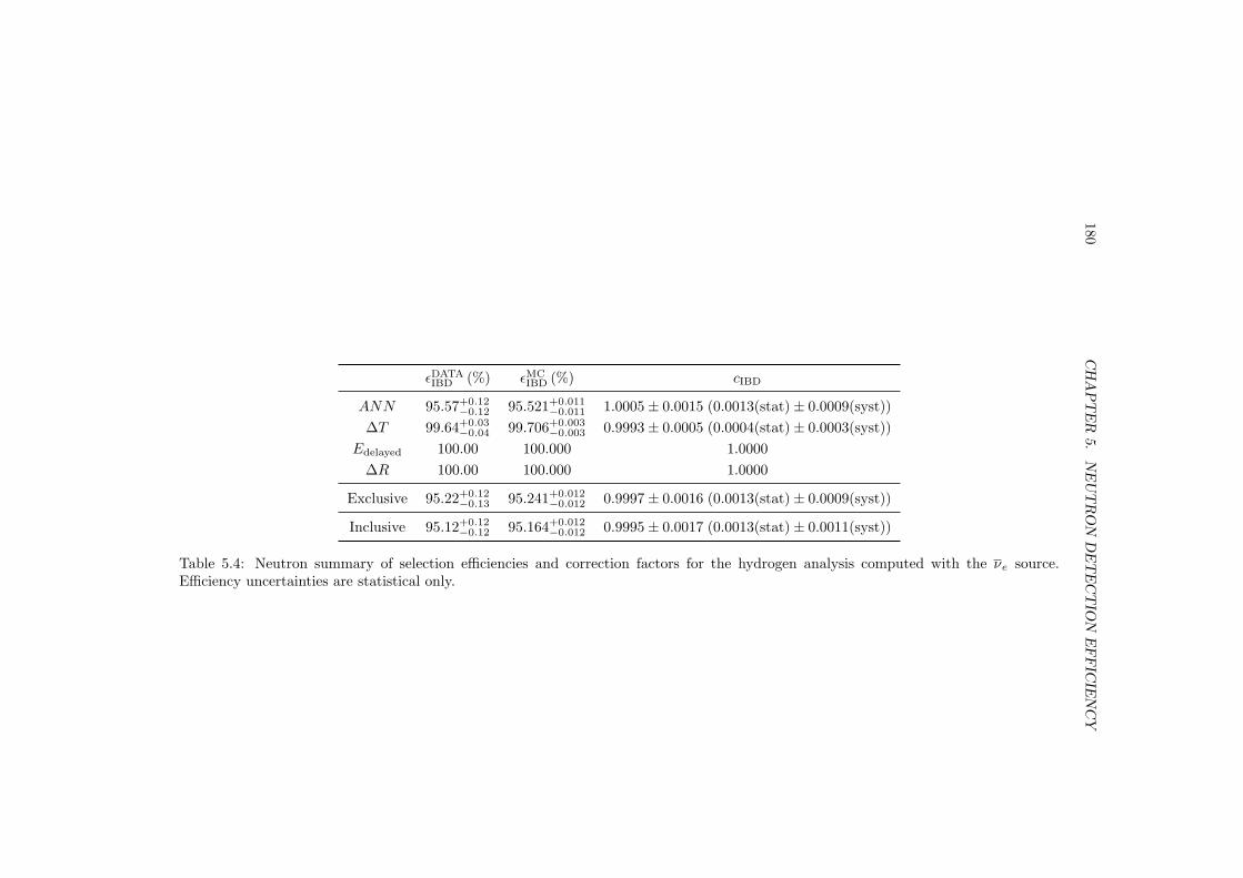
180C
HA
PT
ER
5.N
EU
TR
ON
DE
TE
CT
ION
EFFIC
IEN
CY
εDATAIBD (%) εMC
IBD (%) cIBD
ANN 95.57+0.12−0.12 95.521+0.011
−0.011 1.0005± 0.0015 (0.0013(stat)± 0.0009(syst))∆T 99.64+0.03
−0.04 99.706+0.003−0.003 0.9993± 0.0005 (0.0004(stat)± 0.0003(syst))
Edelayed 100.00 100.000 1.0000∆R 100.00 100.000 1.0000
Exclusive 95.22+0.12−0.13 95.241+0.012
−0.012 0.9997± 0.0016 (0.0013(stat)± 0.0009(syst))
Inclusive 95.12+0.12−0.12 95.164+0.012
−0.012 0.9995± 0.0017 (0.0013(stat)± 0.0011(syst))
Table 5.4: Neutron summary of selection efficiencies and correction factors for the hydrogen analysis computed with the νe source.Efficiency uncertainties are statistical only.
5.5. NEUTRON DETECTION IN THE HYDROGEN SELECTION 181
where NTdet corresponds to events which have both the positron and the neutron
contained within the Target. Φintdet, the internal spill events, corresponds to spill
events occurring in the Target-Gamma Catcher interface, or in the Target vessel.NGC
det represents the number of events with the two signals inside the GammaCatcher. Φext
det, the external spill events, corresponds to any spill event involvingthe Gamma Catcher vessel or the Buffer.
The strategy to estimate the normalization uncertainty due to the neutronmigration relies on the comparison between the two simulations, Geant4 andTripoli4, as it did for the Gd case (section 5.4.3). As it was stated before,Tripoli4 does not feature a model of the detector response, so the prompt anddelayed visible energies or the reconstructed vertices are not available. This rep-resents a significant shortcoming since the reconstructed variables Edelayed, ∆T ,∆R are needed to produce the ANN value which is used in the selection. Inorder to emulate the reconstruction with Tripoli4, detector response maps forthe Edelayed and ∆R variables were built using the reconstructed Geant4 simu-lation (the timing information can be taken directly from the truth informationsince it is very similar to the reconstructed one though). Those maps are binnedunevenly to provide more granularity in the position dependence close to thevolume boundaries, where those variables vary the most. Thus, for a Tripoli4neutron captured in a certain location, a Edelayed and ∆R 6 values are randomlygenerated for it according to the Geant4 distributions at that spatial bin. Theseprocedure is iterated 10000 times to minimize the statistical fluctuations.
In order to calculate the number of the detected events in equation 5.61, theνe from both MC simulations are selected using the H selection cuts (sec. 4.2.2).Moreover, to ensure the likeness between the DATA and the MC, the Geant4normalizations are corrected using the hydrogen fraction and neutron selectionefficiency corrections factors found in the previous sections. The discrepancies inthe number of spill events between the Geant4 and Tripoli4 simulations foundare 0.04% for the internal spill, and 0.13% for the external spill; both expressedrelative to the total normalization of detected events in Geant4. While it is truethat the candidate selection and the neutron selection efficiency are computedwithout making any distinction about where the neutron is captured, the factthat such distinction is made to apply the hydrogen correction factor makesnecessary to account for the uncertainty introduced by the internal spill events,in addition to the external spill. Thus, the discrepancy between simulationsin the global spill class (the sum of the internal and external spills), 0.18%, isconsidered as the normalization uncertainty caused by the modelization of theneutron migration.
There are additional statistical uncertainties arising from the size of theMC samples used to estimate the discrepancy (0.03%) and from the emulationof the detector response in Tripoli4, which is estimated from the standarddeviations of the resulting distributions of the number of spill events after the10000 iterations. The latter is found to amount to 0.02% of the Geant4 selectedνe.
In order to address a possible systematic bias stemming from the emulationof the detector response, the discrepancy between Geant4 and Tripoli4 spillnumbers is recomputed correcting the Tripoli4 simulation with the detection
6Specifically, for ∆R, what it is generated is a shift, δR, from the Geant4 reconstructed∆R - true ∆R distribution, which is then added to the true ∆R from Tripoli4.
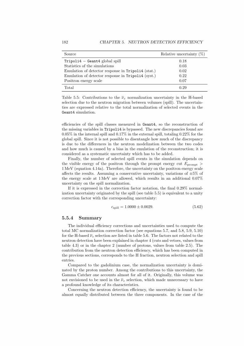
182 CHAPTER 5. NEUTRON DETECTION EFFICIENCY
Source Relative uncertainty (%)
Tripoli4 − Geant4 global spill 0.18Statistics of the simulations 0.03Emulation of detector response in Tripoli4 (stat.) 0.02Emulation of detector response in Tripoli4 (syst.) 0.22Positron energy scale 0.07
Total 0.29
Table 5.5: Contributions to the νe normalization uncertainty in the H-basedselection due to the neutron migration between volumes (spill). The uncertain-ties are expressed relative to the total normalization of selected events in theGeant4 simulation.
efficiencies of the spill classes measured in Geant4, so the reconstruction ofthe missing variables in Tripoli4 is bypassed. The new discrepancies found are0.05% in the internal spill and 0.17% in the external spill, totaling 0.22% for theglobal spill. Since it is not possible to disentangle how much of the discrepancyis due to the differences in the neutron modelization between the two codesand how much is caused by a bias in the emulation of the reconstruction; it isconsidered as a systematic uncertainty which has to be added.
Finally, the number of selected spill events in the simulation depends onthe visible energy of the positron through the prompt energy cut Eprompt >1 MeV (equation 4.14a). Therefore, the uncertainty on the positron energy scaleaffects the results. Assuming a conservative uncertainty, variations of ±5% ofthe energy scale at 1 MeV are allowed, which results in an additional 0.07%uncertainty on the spill normalization.
If it is expressed in the correction factor notation, the final 0.29% normal-ization uncertainty originated by the spill (see table 5.5) is equivalent to a unitycorrection factor with the corresponding uncertainty:
cspill = 1.0000± 0.0029. (5.62)
5.5.4 Summary
The individual efficiency corrections and uncertainties used to compute thetotal MC normalization correction factor (see equations 5.7, and 5.8, 5.9, 5.10)for the H-based νe selection are listed in table 5.6. The factors not related to theneutron detection have been explained in chapter 4 (cuts and vetoes, values fromtable 4.3) or in the chapter 2 (number of protons, values from table 2.5). Thecontribution from the neutron detection efficiency, which has been computed inthe previous sections, corresponds to the H fraction, neutron selection and spillentries.
Compared to the gadolinium case, the normalization uncertainty is domi-nated by the proton number. Among the contributions to this uncertainty, theGamma Catcher one accounts almost for all of it. Originally, this volume wasnot envisioned to be used in the νe selection, which made unnecessary to havea profound knowledge of its characteristics.
Concerning the neutron detection efficiency, the uncertainty is found to bealmost equally distributed between the three components. In the case of the
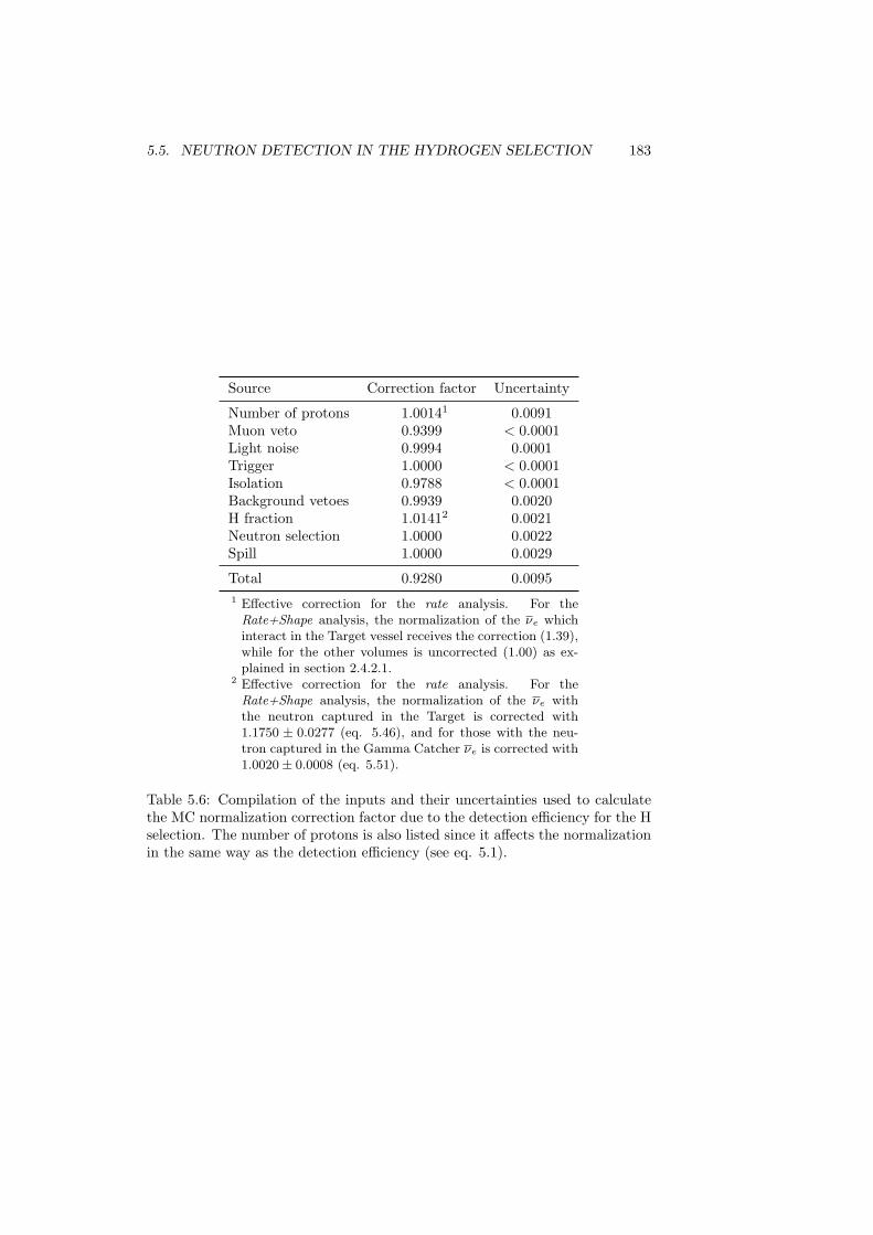
5.5. NEUTRON DETECTION IN THE HYDROGEN SELECTION 183
Source Correction factor Uncertainty
Number of protons 1.00141 0.0091Muon veto 0.9399 < 0.0001Light noise 0.9994 0.0001Trigger 1.0000 < 0.0001Isolation 0.9788 < 0.0001Background vetoes 0.9939 0.0020H fraction 1.01412 0.0021Neutron selection 1.0000 0.0022Spill 1.0000 0.0029
Total 0.9280 0.00951 Effective correction for the rate analysis. For the
Rate+Shape analysis, the normalization of the νe whichinteract in the Target vessel receives the correction (1.39),while for the other volumes is uncorrected (1.00) as ex-plained in section 2.4.2.1.
2 Effective correction for the rate analysis. For theRate+Shape analysis, the normalization of the νe withthe neutron captured in the Target is corrected with1.1750 ± 0.0277 (eq. 5.46), and for those with the neu-tron captured in the Gamma Catcher νe is corrected with1.0020± 0.0008 (eq. 5.51).
Table 5.6: Compilation of the inputs and their uncertainties used to calculatethe MC normalization correction factor due to the detection efficiency for the Hselection. The number of protons is also listed since it affects the normalizationin the same way as the detection efficiency (see eq. 5.1).
184 CHAPTER 5. NEUTRON DETECTION EFFICIENCY
H-fraction correction, the uncertainty comes mainly from the Target. In theTarget scintillator, the H captures are the alternative to Gd captures, so the Hfraction is affected by the uncertainty on the Gd fraction (which is the mainuncertainty in the Gd analysis). Nevertheless, the fact that 89.5% of the cap-tures on H nuclei occur in the Gamma Catcher, where the H fraction is preciselymeasured, alleviates the lack of knowledge in the Target. The neutron selectionefficiency correction shows an uncertainty very similar to the Gd analysis, whichis expected since the same methods using the νe source have been used in bothanalyses. The spill has also a similar uncertainty since both H and Gd estima-tions rely on the comparison between the Geant4 and Tripoli4 simulations.
Regarding the outlook for the two-detector phase, it must be noted that sincethe Gamma Catcher was not planned to be used as a νe detection volume, theliquid scintillator used for the Near Detector Gamma Catcher does not comefrom the same batch as the Far Detector one, unlike the Target scintillator.Therefore, the uncertainty due to the proton number on the Gamma Catcheris not expected to cancel in the two-detector phase. However, an improvementon this uncertainty is expected (reaching & 0.4%) because of the measurementsmade during the Near Detector filling and provided that only relative differencesbetween detectors are relevant in this phase.
On the contrary, the H fraction uncertainty benefits from the two-detectorphase because it is driven by the Target scintillator, which is identical for bothdetectors; so the only uncorrelated component is the statistical one, which canbe made negligible with dedicated calibration.
Since the measurement of the neutron selection efficiency has an uncertaintyvery similar to the Gd one, the same considerations apply. This uncertainty isuncorrelated between detectors, so it is still relevant in the two-detector phase.The statistical component, which makes up half of the uncertainty, will decreaseas more antineutrino data is acquired. It must be noted that the proximity of theNear Detector to the reactor cores allows it to gain antineutrino data faster thanthe Far Detector, so the dominant statistical uncertainty after a few months isthe Far Detector one. The systematic component arises from the stopping muoncontamination, so it can be reduced if new vetoes are devised.
Finally, in the two-detector phase the pertinent spill uncertainty is due todifferences between the real detectors rather than between the simulations, andit is expected to be almost negligible.
Chapter 6
Oscillation analysis andmeasurement of θ13
After the selection of IBD candidates in the DATA and MC has been per-formed according to the cuts described in chapter 4, with an estimation ofthe backgrounds contaminating the DATA using the techniques explained inthe same chapter, and the normalization of the MC νe simulation has beencorrected with the factors described extensively in chapter 5; the number ofobserved IBD candidates can be compared to the prediction (see table 6.1). Inboth selections using neutron captures either on Gd or on H, a deficit with re-spect to the prediction is found. This deficit of IBD interactions is interpretedas the result of electron antineutrino conversion to other flavors driven by theθ13 mixing angle.
In order to exploit the signal information and distinguish it from the back-ground with the goal of providing a precise measurement of θ13, the νe deficitis studied as a function of the reactor thermal power (Reactor Rate Modula-tion analysis, section 6.1) or as a function of the prompt trigger visible energy(Rate+Shape analysis, section 6.2). Finally, the chapter concludes with theprospective improvement to the measure of θ13 brought by the inclusion of theNear Detector (section 6.3).
6.1 Reactor Rate Modulation analysis
The Reactor Rate Modulation (RRM) analysis [74] is based on the factthat while the νe interaction rate scales with the reactor thermal power, thebackground rate remains constant. This allows to disentangle the contributionof the background to the observed IBD candidate rate from that of the νe, whichis the only affected by the value of θ13.
The observed rate can be expressed as
Robs = B +(1− sin2(2θ13)ηosc
)Rν , (6.1)
where B is the background rate and Rν is the expected rate of νe if there werenot oscillation (given by equation 2.7). ηosc is the oscillatory factor of equation1.54 averaged over the energies and baselines of the νe emitted by the reactor
185
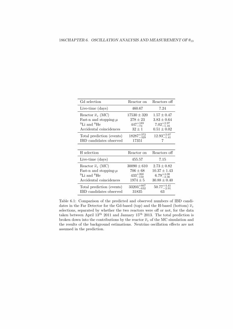
186CHAPTER 6. OSCILLATION ANALYSIS AND MEASUREMENT OF θ13
Gd selection Reactor on Reactors off
Live-time (days) 460.67 7.24
Reactor νe (MC) 17530± 320 1.57± 0.47Fast-n and stopping-µ 278± 23 3.83± 0.649Li and 8He 447+189
−74 7.02+2.97−1.16
Accidental coincidences 32± 1 0.51± 0.02
Total prediction (events) 18287+372−329 12.93+3.07
−1.41
IBD candidates observed 17351 7
H selection Reactor on Reactors off
Live-time (days) 455.57 7.15
Reactor νe (MC) 30090± 610 2.73± 0.82Fast-n and stopping-µ 706± 68 10.37± 1.439Li and 8He 433+260
−150 6.79+4.08−2.36
Accidental coincidences 1974± 5 30.88± 0.40
Total prediction (events) 33203+667−632 50.77+4.41
−2.91
IBD candidates observed 31835 63
Table 6.1: Comparison of the predicted and observed numbers of IBD candi-dates in the Far Detector for the Gd-based (top) and the H-based (bottom) νeselections, separated by whether the two reactors were off or not, for the datataken between April 13th 2011 and January 15th 2013. The total prediction isbroken down into the contributions by the reactor νe of the MC simulation andthe results of the background estimations. Neutrino oscillation effects are notassumed in the prediction.
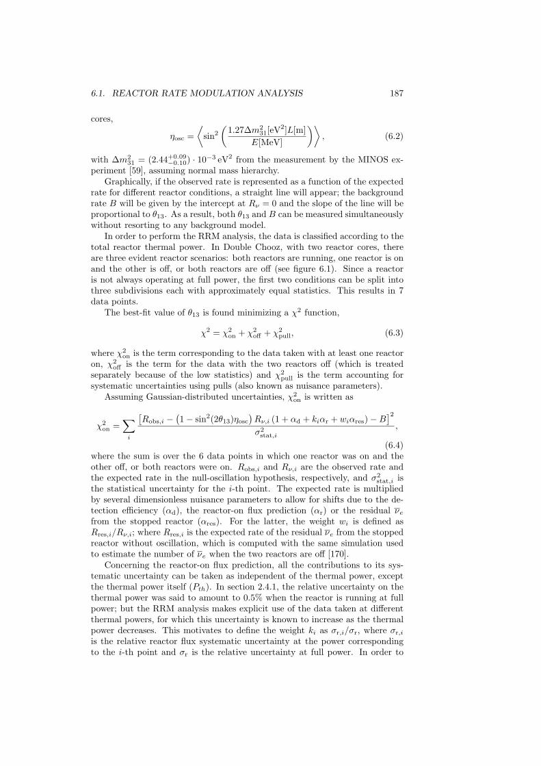
6.1. REACTOR RATE MODULATION ANALYSIS 187
cores,
ηosc =⟨
sin2
(1.27∆m2
31[eV2]L[m]E[MeV]
)⟩, (6.2)
with ∆m231 = (2.44+0.09
−0.10) · 10−3 eV2 from the measurement by the MINOS ex-periment [59], assuming normal mass hierarchy.
Graphically, if the observed rate is represented as a function of the expectedrate for different reactor conditions, a straight line will appear; the backgroundrate B will be given by the intercept at Rν = 0 and the slope of the line will beproportional to θ13. As a result, both θ13 and B can be measured simultaneouslywithout resorting to any background model.
In order to perform the RRM analysis, the data is classified according to thetotal reactor thermal power. In Double Chooz, with two reactor cores, thereare three evident reactor scenarios: both reactors are running, one reactor is onand the other is off, or both reactors are off (see figure 6.1). Since a reactoris not always operating at full power, the first two conditions can be split intothree subdivisions each with approximately equal statistics. This results in 7data points.
The best-fit value of θ13 is found minimizing a χ2 function,
χ2 = χ2on + χ2
off + χ2pull, (6.3)
where χ2on is the term corresponding to the data taken with at least one reactor
on, χ2off is the term for the data with the two reactors off (which is treated
separately because of the low statistics) and χ2pull is the term accounting for
systematic uncertainties using pulls (also known as nuisance parameters).Assuming Gaussian-distributed uncertainties, χ2
on is written as
χ2on =
∑i
[Robs,i −
(1− sin2(2θ13)ηosc
)Rν,i (1 + αd + kiαr + wiαres)−B
]2σ2
stat,i
,
(6.4)where the sum is over the 6 data points in which one reactor was on and theother off, or both reactors were on. Robs,i and Rν,i are the observed rate andthe expected rate in the null-oscillation hypothesis, respectively, and σ2
stat,i isthe statistical uncertainty for the i-th point. The expected rate is multipliedby several dimensionless nuisance parameters to allow for shifts due to the de-tection efficiency (αd), the reactor-on flux prediction (αr) or the residual νefrom the stopped reactor (αres). For the latter, the weight wi is defined asRres,i/Rν,i; where Rres,i is the expected rate of the residual νe from the stoppedreactor without oscillation, which is computed with the same simulation usedto estimate the number of νe when the two reactors are off [170].
Concerning the reactor-on flux prediction, all the contributions to its sys-tematic uncertainty can be taken as independent of the thermal power, exceptthe thermal power itself (Pth). In section 2.4.1, the relative uncertainty on thethermal power was said to amount to 0.5% when the reactor is running at fullpower; but the RRM analysis makes explicit use of the data taken at differentthermal powers, for which this uncertainty is known to increase as the thermalpower decreases. This motivates to define the weight ki as σr,i/σr, where σr,i
is the relative reactor flux systematic uncertainty at the power correspondingto the i-th point and σr is the relative uncertainty at full power. In order to
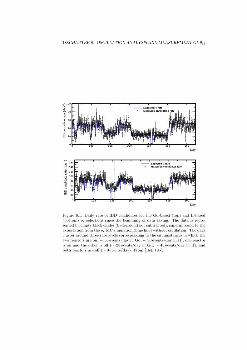
188CHAPTER 6. OSCILLATION ANALYSIS AND MEASUREMENT OF θ13
Day0 100 200 300 400 500 600
)-1
IBD
can
dida
te r
ate
(day
0
20
40
60
80
100
rateνExpected Measured candidates rate
Day0 100 200 300 400 500 600
)-1
IBD
can
dida
te r
ate
(day
0
20
40
60
80
100
120
140
160 rateνExpected Measured candidates rate
Figure 6.1: Daily rate of IBD candidates for the Gd-based (top) and H-based(bottom) νe selections since the beginning of data taking. The data is repre-sented by empty black circles (background not subtracted), superimposed to theexpectation from the νe MC simulation (blue line) without oscillation. The datacluster around three rate levels corresponding to the circumstances in which thetwo reactors are on (∼ 50 events/day in Gd, ∼ 90 events/day in H), one reactoris on and the other is off (∼ 25 events/day in Gd, ∼ 45 events/day in H), andboth reactors are off (∼ 0 events/day). From [164, 195].
6.1. REACTOR RATE MODULATION ANALYSIS 189
estimate σr,i, an empirical model is fitted to a set of measurements made by thepower plant operators. This results in a 1/Pth dependence, with a maximumσr,i = 1.9% when either one or the two reactors are not at full power and aminimum of σr,i = σr = 1.7% when both are running at full power.
For the two reactors off period, as a result of the low number of events, χ2off
is built as a binned Poisson extended likelihood:
χ2off = 2
[Nobs ln
(Nobs
Nexp
)+Nexp −Nobs
], (6.5)
where Nobs is the number of IBD candidates observed in the reactors-off sample(see table 6.1); and the expectation is given by
Nexp =[(
1− sin2(2θ13)ηosc
)Rres,off (1 + αd + αres) +B
]· Toff ,
where Rres,off is the expected rate of residual νe from the two stopped reactorsin absence of oscillation and Toff is the total live-time of the reactors-off period.
Finally, χ2pull, the term for the systematic uncertainties is written as
χ2pull =
(αd
σd
)2
+(αr
σr
)2
+(αres
σres
)2
, (6.6)
where σd is the relative uncertainty on the detection efficiency (0.63% for theGd-based νe selection, from table 5.3; and 1.02% for the H-based, from table 5.6)and σres is the relative uncertainty on the rate of residual νe from the stoppedreactor, which amounts to 30% (cf. table 6.1). The systematic uncertainty onthe reactor-on flux, already introduced above (σr = 1.7%), is considered conser-vatively as correlated between the data points since the dominant contributionis the uncertainty on the measurement of the mean cross-section per fission bythe Bugey4 experiment [144], which is independent of the thermal power.
Notice that so far, the background rate B is a free parameter. This is oneof the most remarkable features of the RRM analysis, that is, it is capable ofmeasuring the total background rate in a background-model-independent way.
Alternatively, in order to exploit all the information available to produce themost precise measurement of θ13; Bexp, the total background rate estimationarising from the individual estimations using the IBD candidate DATA (table4.2 for the Gd selection, table 4.4 for the H selection) can be included in the fitat the expense of losing the background-model independence. In this case, χ2
pull
is
χ2pull =
(αd
σd
)2
+(αr
σr
)2
+(αres
σres
)2
+(B −Bexp
σB
)2
, (6.7)
where σB is the uncertainty on Bexp.
6.1.1 Gd results
After introducing the fundamentals of the RRM analysis in the previoussection, it can be applied to the particular case of the Gd-based νe selection.
Firstly, in order to obtain a measurement of θ13 independent of the back-ground model, B is treated as a free parameter. A global scan is executed on thesin2(2θ13)−B plane, in which the χ2 (see equation 6.3, with χ2
pull given by equa-tion 6.6) is minimized at each point with respect to the three nuisance parame-ters (αd, αr, αres). The minimum χ2 value is found at sin2(2θ13) = 0.060±0.039
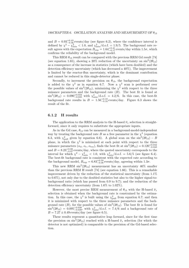
190CHAPTER 6. OSCILLATION ANALYSIS AND MEASUREMENT OF θ13
and B = 0.93+0.43−0.36 events/day (see figure 6.2), where the confidence interval is
defined by χ2 − χ2min < 1.0, and χ2
min/d.o.f. = 1.9/5. The background rate re-sult agrees with the expectation Bexp = 1.64+0.41
−0.17 events/day within 1.5σ, whichconfirms the reliability of the background model.
This RRM θ13 result can be compared with the previous RRM Gd result [74](see equation 1.65), showing a 20% reduction of the uncertainty on sin2(2θ13)as a consequence of the increase in statistics (which have been doubled) and thedetection efficiency uncertainty (which has decreased a 40%). The improvementis limited by the reactor-flux uncertainty, which is the dominant contributionand cannot be reduced in this single-detector phase.
Secondly, to increment the precision on θ13, the background expectationis added to the χ2 as in equation 6.7. Now a χ2 scan is performed overthe possible values of sin2(2θ13), minimizing the χ2 with respect to the threenuisance parameters and the background rate (B). The best fit is found atsin2(2θ13) = 0.090+0.034
−0.035 with χ2min/d.o.f. = 4.2/6. In this case, the best-fit
background rate results in B = 1.56+0.18−0.16 events/day. Figure 6.3 shows the
result of the fit.
6.1.2 H results
The application to the RRM analysis to the H-based νe selection is straight-forward, since it only requires to substitute the appropriate inputs.
As in the Gd case, θ13 can be measured in a background-model-independentway by treating the background rate B as a free parameter in the χ2 (equation6.3, with χ2
pull given by equation 6.6). A global scan on the sin2(2θ13) − B
plane, in which the χ2 is minimized at each point with respect to the threenuisance parameters (αd, αr, αres), finds the best fit at sin2(2θ13) = 0.120+0.042
−0.043
and B = 8.23+0.88−0.87 events/day, where the quoted uncertainty corresponds to the
interval for which χ2 − χ2min < 1.0, with χ2
min/d.o.f. = 5.6/5 (see figure 6.4).The best-fit background rate is consistent with the expected rate according tothe background model, Bexp = 6.83+0.59
−0.36 events/day, agreeing within 1.3σ.This new RRM sin2(2θ13) measurement has an uncertainty 46% smaller
than the previous RRM H result [74] (see equation 1.66). This is a remarkableimprovement driven by the reduction of the statistical uncertainty (from 1.1%to 0.6%), not only due to the doubled statistics but also to the higher signal-to-background ratio (which has passed from 0.9 to 9.7); and the reduction of thedetection efficiency uncertainty (from 1.6% to 1.02%).
However, the most precise RRM measurement of θ13 with the H-based νeselection is obtained when the background rate is constrained by the estima-tion. In this case, the χ2 is built using the χ2
pull from equation 6.7; and thenit is minimized with respect to the three nuisance parameters and the back-ground rate (B), for the possible values of sin2(2θ13). The best fit is found forsin2(2θ13) = 0.095+0.038
−0.039, with χ2min/d.o.f. = 7.4/6 and a background rate of
B = 7.27± 0.49 events/day (see figure 6.5).These results represent a quantitative leap forward, since for the first time
the precision on sin2(2θ13) reached with a H-based νe selection (for which thedetector is not optimized) is comparable to the precision of the Gd-based selec-tion.
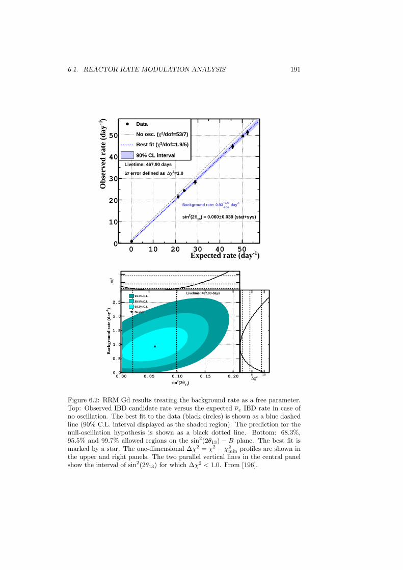
6.1. REACTOR RATE MODULATION ANALYSIS 191
)-1Expected rate (day0 10 20 30 40 50
)-1
Obs
erve
d ra
te (
day
0
10
20
30
40
50
Data
/dof=53/7)2χNo osc. (
/dof=1.9/5)2χBest fit (
90% CL interval
Data
/dof=53/7)2χNo osc. (
/dof=1.9/5)2χBest fit (
90% CL interval
Data
/dof=53/7)2χNo osc. (
/dof=1.9/5)2χBest fit (
90% CL interval
Livetime: 467.90 days
=1.02χ∆ error defined as σ1
-1 day-0.36
+0.43Background rate: 0.93
0.039 (stat+sys)±) = 0.06013θ(22sin
)13
θ(22sin0.00 0.05 0.10 0.15 0.20
2 χ∆ 5
10
)13
θ(22sin
0.00 0.05 0.10 0.15 0.20
)-1
Bac
kgro
und
rate
(da
y
0.0
0.5
1.0
1.5
2.0
2.5
Livetime: 467.90 days99.7% C.L.
95.5% C.L.
68.3% C.L.
Best-fit
2χ∆5 10
Bac
kgro
und
(eve
nts/
day)
0.0
0.5
1.0
1.5
2.0
2.5
Figure 6.2: RRM Gd results treating the background rate as a free parameter.Top: Observed IBD candidate rate versus the expected νe IBD rate in case ofno oscillation. The best fit to the data (black circles) is shown as a blue dashedline (90% C.L. interval displayed as the shaded region). The prediction for thenull-oscillation hypothesis is shown as a black dotted line. Bottom: 68.3%,95.5% and 99.7% allowed regions on the sin2(2θ13) − B plane. The best fit ismarked by a star. The one-dimensional ∆χ2 = χ2 − χ2
min profiles are shown inthe upper and right panels. The two parallel vertical lines in the central panelshow the interval of sin2(2θ13) for which ∆χ2 < 1.0. From [196].
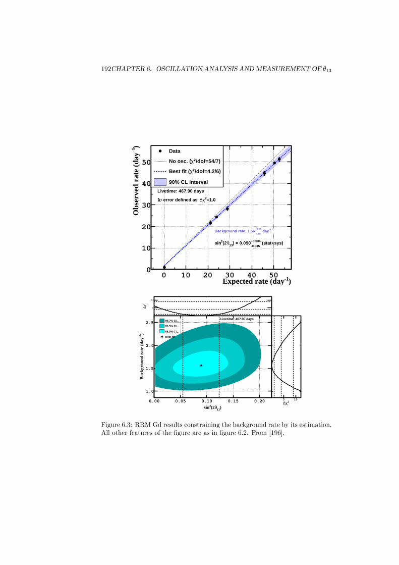
192CHAPTER 6. OSCILLATION ANALYSIS AND MEASUREMENT OF θ13
)-1Expected rate (day0 10 20 30 40 50
)-1
Obs
erve
d ra
te (
day
0
10
20
30
40
50
Data
/dof=54/7)2χNo osc. (
/dof=4.2/6)2χBest fit (
90% CL interval
Data
/dof=54/7)2χNo osc. (
/dof=4.2/6)2χBest fit (
90% CL interval
Data
/dof=54/7)2χNo osc. (
/dof=4.2/6)2χBest fit (
90% CL interval
Livetime: 467.90 days
=1.02χ∆ error defined as σ1
-1 day-0.16
+0.18Background rate: 1.56
(stat+sys)-0.035
+0.034) = 0.09013θ(22sin
)13
θ(22sin0.00 0.05 0.10 0.15 0.20
2 χ∆ 5
10
)13
θ(22sin
0.00 0.05 0.10 0.15 0.20
)-1
Bac
kgro
und
rate
(da
y
1.0
1.5
2.0
2.5Livetime: 467.90 days
99.7% C.L.
95.5% C.L.
68.3% C.L.
Best-fit
2χ∆5 10
Bac
kgro
und
(eve
nts/
day)
1.0
1.5
2.0
2.5
Figure 6.3: RRM Gd results constraining the background rate by its estimation.All other features of the figure are as in figure 6.2. From [196].
6.1. REACTOR RATE MODULATION ANALYSIS 193
)-1Expected rate (day0 20 40 60 80
)-1
Obs
erve
d ra
te (
day
0
20
40
60
80
100 Data
/dof=58/7)2χNo osc.(
/dof=5.6/5)2χBest fit (
90% CL
Livetime: 462.72 days
=1.02χ∆ error defined as σ1
-1 day-0.87
+0.88Background rate: 8.23
(stat+sys)-0.043
+0.042) = 0.12013θ(22sin
)13
θ(22sin0.00 0.05 0.10 0.15 0.20 0.25
2 χ∆ 5
10
)13
θ(22sin
0.00 0.05 0.10 0.15 0.20 0.25
)-1
Bac
kgro
und
rate
(da
y
5
6
7
8
9
10
11Livetime: 462.72 days99.7% C.L.
95.5% C.L.
68.3% C.L.
Best-fit
2χ∆0 5 10
Bac
kgro
und
(eve
nts/
day)
5
6
7
8
9
10
11
Figure 6.4: RRM H results treating the background rate as a free parameter.Top: Observed IBD candidate rate versus the expected νe IBD rate in case ofno oscillation. The best fit to the data (black circles) is shown as a blue dashedline (90% C.L. interval displayed as the shaded region). The prediction for thenull-oscillation hypothesis is shown as a black dotted line. Bottom: 68.3%,95.5% and 99.7% allowed regions on the sin2(2θ13) − B plane. The best fit ismarked by a star. The one-dimensional ∆χ2 = χ2 − χ2
min profiles are shown inthe upper and right panels. The two parallel vertical lines in the central panelshow the interval of sin2(2θ13) for which ∆χ2 < 1.0. From [197].
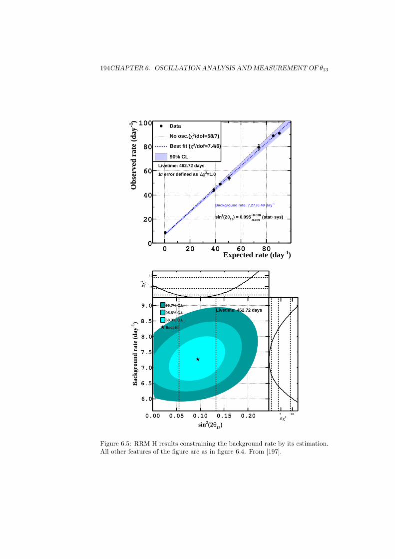
194CHAPTER 6. OSCILLATION ANALYSIS AND MEASUREMENT OF θ13
)-1Expected rate (day0 20 40 60 80
)-1
Obs
erve
d ra
te (
day
0
20
40
60
80
100 Data
/dof=58/7)2χNo osc.(
/dof=7.4/6)2χBest fit (
90% CL
Livetime: 462.72 days
=1.02χ∆ error defined as σ1
-10.49 day±Background rate: 7.27
(stat+sys)-0.039
+0.038) = 0.09513θ(22sin
)13
θ(22sin0.00 0.05 0.10 0.15 0.20
2 χ∆ 5
10
)13
θ(22sin
0.00 0.05 0.10 0.15 0.20
)-1
Bac
kgro
und
rate
(da
y
6.0
6.5
7.0
7.5
8.0
8.5
9.0
DC-III (nH) Preliminary
Livetime: 462.72 days99.7% C.L.
95.5% C.L.
68.3% C.L.
Best-fit
2χ∆5 10
Bac
kgro
und
(eve
nts/
day)
6.0
6.5
7.0
7.5
8.0
8.5
9.0
Figure 6.5: RRM H results constraining the background rate by its estimation.All other features of the figure are as in figure 6.4. From [197].
6.1. REACTOR RATE MODULATION ANALYSIS 195
6.1.3 Combined Gd and H results
In order to boost the precision on the measurement of θ13, the RRM analysiscan be performed simultaneously over the Gd and H data sets. The χ2 decom-position (equation 6.3) into three terms can be kept; with χ2
on, χ2off and χ2
pull
corresponding to data with at least one reactor on, data with the two reactorsoff and a specific term for the systematic uncertainties, respectively. But eachterm must be modified with respect to the previous section to accommodate thetwo νe selections.
The χ2on for the combined Gd and H fit is written as
χ2on =
=∑i
[RGd
obs,i − 〈Psurv〉RGdν,i
(1 + αGd,unc
d + αcord + kiαr + wiαres
)−BGd
]2σ2
stat,i
+
+∑j
[RH
obs,j − 〈Psurv〉RHν,j
(1 + αH,unc
d + αcord + kjαr + wjαres
)−BH
]2σ2
stat,j
,
(6.8)
where the summation index i runs over the 6 data points of the Gd selection,and the summation index j runs over the 6 data points of the H selection.Notice that this χ2
on is not a mere duplication of that from equation 6.4: besidesthe oscillation parameters of the averaged survival probability 〈Psurv〉 = (1 −sin2(2θ13)ηosc) which must be the same regardless the nuclei chosen to capturethe IBD neutron, the nuisance parameters for the reactor-on flux prediction(αr) and the residual νe from the stopped reactor (αres) are also the same forthe Gd and H terms. This is due to the fact that both parameters refer onlyto the reactor simulations, which are shared by the two νe selections, so thesystematic uncertainties associated to them are fully correlated. In addition, foreach νe selection, the nuisance parameter accounting for the detection efficiencyin equation 6.4 has been replaced by two parameters, one which is selection-dependent to allow for uncorrelated shifts (αX,unc
d , where X is Gd or H) andanother which is common to both selections to describe the correlated effects(αcor
d ).The χ2
off is simplyχ2
off = χ2off,Gd + χ2
off,H, (6.9)
where each term is given by equation 6.5, except that the expected number ofevents is changed to
NXexp =
[(1− sin2(2θ13)ηosc
)RXres,off
(1 + αX,unc
d + αcord + αres
)+BX
]· TXoff ,
where X denotes the Gd or H variables.Finally, the term for the systematic uncertainties can be written in two
different forms, depending on whether the background rates BGd and BH aretreated as free parameters or not. On the one hand, if they are treated asfree parameters, then the analysis is background-model independent and χ2
pull
is written
χ2pull =
(αGd,unc
d
σGd,uncd
)2
+
(αH,unc
d
σH,uncd
)2
+(αcor
d
σcord
)2
+(αr
σr
)2
+(αres
σres
)2
, (6.10)
196CHAPTER 6. OSCILLATION ANALYSIS AND MEASUREMENT OF θ13
where σGd,uncd and σH,unc
d are the uncorrelated relative uncertainties on thedetection efficiency of the Gd and H selections, respectively; and σcor
d is thecorrelated component. Their specific values depend on the degree of correlationestimated.
In this case, a global scan over the three-dimensional space defined bysin2(2θ13), BGd and BH is carried out, in which the χ2 is minimized with respectto the five nuisance parameters (αGd,unc
d , αH,uncd , αcor
d , αr, αres). Initially, thedetection efficiency uncertainties are considered to be fully uncorrelated, whichis equivalent to fixing αcor
d to zero and σGd,uncd = σGd
d and σH,uncd = σH
d . Theminimum χ2 is found at sin2(2θ13) = 0.075±0.037, BGd = 1.21+0.41
−0.38 events/dayand BH = 7.44+0.69
−0.68 events/day (see figure 6.6), where the confidence intervalis defined by χ2 − χ2
min < 1.0, and χ2min/d.o.f. = 10/11. As in the individual
fits, the resulting background rates are in good agreement (within less than1σ) with the background-model expectations: BGd
exp = 1.64+0.41−0.17 events/day and
BHexp = 6.83+0.59
−0.36 events/day. To test the impact of the correlation between thedetection efficiency uncertainties, the analysis was repeated assuming a 30%correlation between the two (the maximum possible because of the detectionvolume shared by the two νe selections) and no effect was observed. This wasforeseen since the systematic uncertainty is largely dominated by the reactorsystematic uncertainty.
The sin2(2θ13) = 0.075±0.037 just obtained is the most precise background-model-independent measurement of θ13, since this analysis is unique from Dou-ble Chooz. This result is 14% more precise than the previous combination ofthe Gd and H data sets [74] (see equation 1.67).
On the other hand, if the goal is to maximize the precision on θ13, then theexpected total background rates from the background models can be includedin the χ2. Henceforth, the background rates are treated as nuisance parameters,and χ2
pull is written as
χ2pull =
(αGd,unc
d
σGd,uncd
)2
+
(αH,unc
d
σH,uncd
)2
+(αcor
d
σcord
)2
+(αr
σr
)2
+(αres
σres
)2
+
+(BGd −BGd
exp, BH −BH
exp
)·
·
((σGd
B )2 ρBσGdB σH
B
ρBσGdB σH
B (σHB )2
)−1(BGd −BGd
exp
BH −BHexp
), (6.11)
where BGdexp and BH
exp are the estimated total background rates for the Gd andH selections, respectively; and σGd
B and σHB their corresponding uncertainties,
with ρB their correlation coefficient.The total χ2 is now minimized with respect to the seven nuisance parameters
(αGd,uncd , αH,unc
d , αcord , αr, αres, BGd, BH). Assuming fully uncorrelated uncer-
tainties on the detection efficiency and the background rates (i.e. ρB = 0), a scanover possible values of sin2(2θ13) finds the best fit at sin2(2θ13) = 0.088±0.033,with χ2
min/d.o.f. = 11/13 (see figure 6.7). The best-fit background rates areBGd = 1.57±0.16 events/day and BH = 7.22±0.43 events/day. Assuming fullycorrelated uncertainties on the detection efficiency or the background rates in-stead has a negligible effect on the θ13 result. Again, this was expected becausethe reactor-flux uncertainty prevails over the rest of the uncertainties.
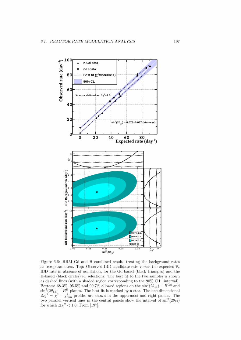
6.1. REACTOR RATE MODULATION ANALYSIS 197
)-1Expected rate (day0 20 40 60 80
)-1
Obs
erve
d ra
te (
day
0
20
40
60
80
100n-Gd data
n-H data
/dof=10/11)2χBest fit (
90% CL
0.037 (stat+sys)±) = 0.07513θ(22sin
=1.02χ∆ error defined as σ1
)13
θ(22sin0.00 0.05 0.10 0.15 0.20
2 χ∆ 5
10
)13
θ(22sin0.00 0.05 0.10 0.15 0.20
)-1
nGd
Bac
kgro
und
rate
(da
y
0.5
1.0
1.5
2.0
2.5
2χ∆5 10
Bac
kgro
und
(eve
nts/
day)
0.0
0.5
1.0
1.5
2.0
2.5
3.0
)13θ(22sin0.00 0.05 0.10 0.15 0.20
)-1
nH B
ackg
roun
d ra
te (
day
5
6
7
8
9
10
99.7% C.L.
95.5% C.L.
68.3% C.L.
Best-fit
2χ∆5 10
Bac
kgro
und
(eve
nts/
day)
5
6
7
8
9
10
Figure 6.6: RRM Gd and H combined results treating the background ratesas free parameters. Top: Observed IBD candidate rate versus the expected νeIBD rate in absence of oscillation, for the Gd-based (black triangles) and theH-based (black circles) νe selections. The best fit to the two samples is shownas dashed lines (with a shaded region corresponding to the 90% C.L. interval).Bottom: 68.3%, 95.5% and 99.7% allowed regions on the sin2(2θ13)−BGd andsin2(2θ13)−BH planes. The best fit is marked by a star. The one-dimensional∆χ2 = χ2 − χ2
min profiles are shown in the uppermost and right panels. Thetwo parallel vertical lines in the central panels show the interval of sin2(2θ13)for which ∆χ2 < 1.0. From [197].
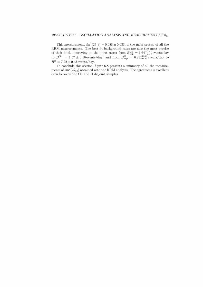
198CHAPTER 6. OSCILLATION ANALYSIS AND MEASUREMENT OF θ13
This measurement, sin2(2θ13) = 0.088± 0.033, is the most precise of all theRRM measurements. The best-fit background rates are also the most preciseof their kind, improving on the input rates: from BGd
exp = 1.64+0.41−0.17 events/day
to BGd = 1.57 ± 0.16 events/day; and from BHexp = 6.83+0.59
−0.36 events/day toBH = 7.22± 0.43 events/day.
To conclude this section, figure 6.8 presents a summary of all the measure-ments of sin2(2θ13) obtained with the RRM analysis. The agreement is excellenteven between the Gd and H disjoint samples.
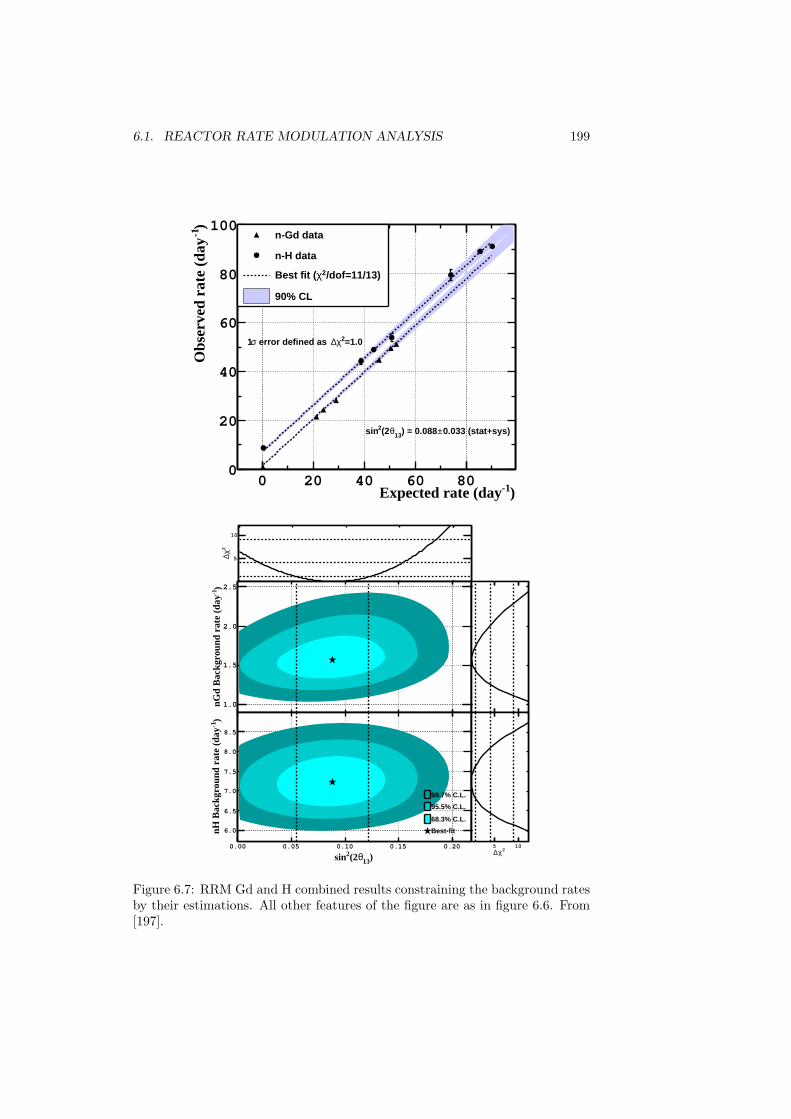
6.1. REACTOR RATE MODULATION ANALYSIS 199
)-1Expected rate (day0 20 40 60 80
)-1
Obs
erve
d ra
te (
day
0
20
40
60
80
100n-Gd data
n-H data
/dof=11/13)2χBest fit (
90% CL
0.033 (stat+sys)±) = 0.08813θ(22sin
=1.02χ∆ error defined as σ1
)13
θ(22sin0.00 0.05 0.10 0.15 0.20
2 χ∆ 5
10
)13
θ(22sin0.00 0.05 0.10 0.15 0.20
)-1
nGd
Bac
kgro
und
rate
(da
y
1.0
1.5
2.0
2.5
2χ∆5 10
Bac
kgro
und
(eve
nts/
day)
1.0
1.5
2.0
2.5
)13θ(22sin0.00 0.05 0.10 0.15 0.20
)-1
nH B
ackg
roun
d ra
te (
day
6.0
6.5
7.0
7.5
8.0
8.5
99.7% C.L.
95.5% C.L.
68.3% C.L.
Best-fit
2χ∆5 10
Bac
kgro
und
(eve
nts/
day)
6.0
6.5
7.0
7.5
8.0
8.5
9.0
Figure 6.7: RRM Gd and H combined results constraining the background ratesby their estimations. All other features of the figure are as in figure 6.6. From[197].
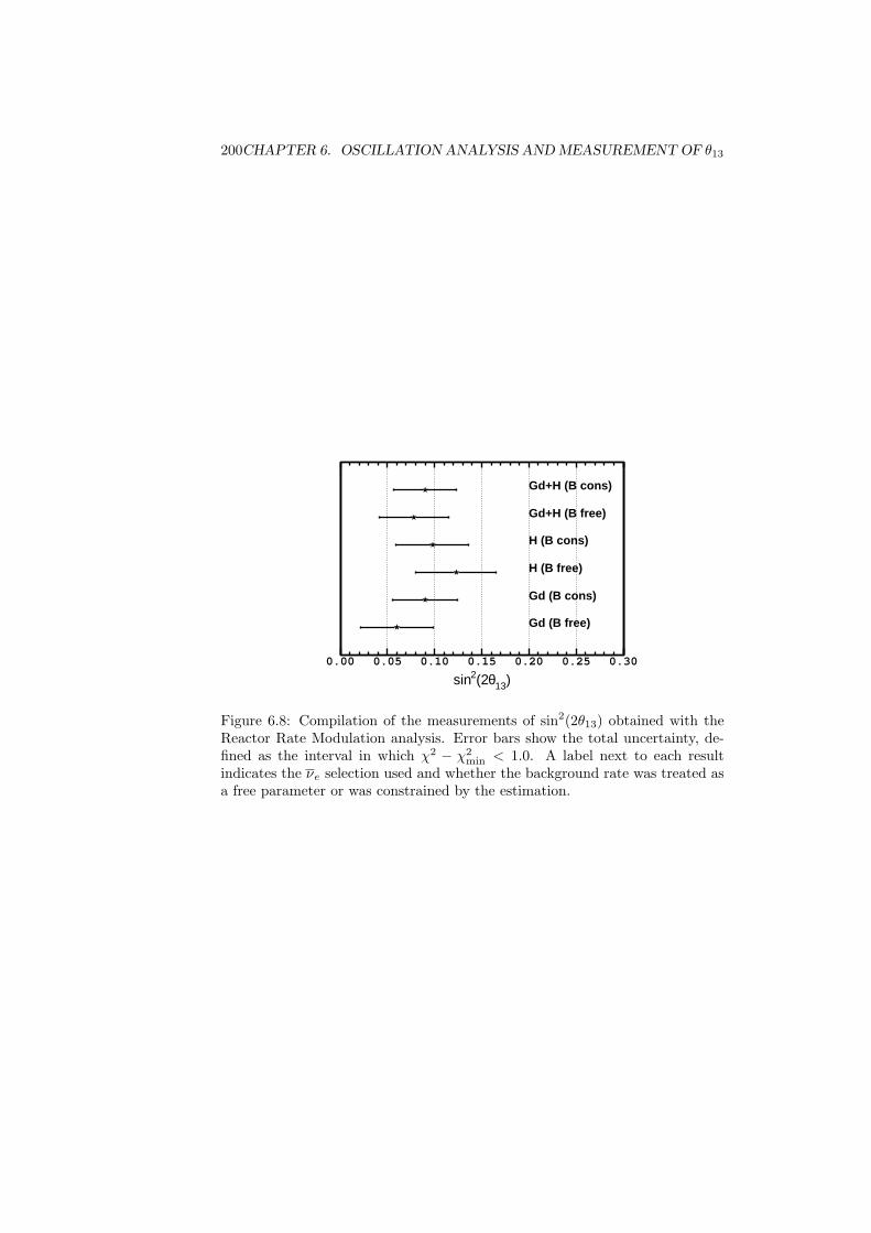
200CHAPTER 6. OSCILLATION ANALYSIS AND MEASUREMENT OF θ13
)13θ(22sin0.00 0.05 0.10 0.15 0.20 0.25 0.30
Gd (B free)
Gd (B cons)
H (B free)
H (B cons)
Gd+H (B free)
Gd+H (B cons)
Figure 6.8: Compilation of the measurements of sin2(2θ13) obtained with theReactor Rate Modulation analysis. Error bars show the total uncertainty, de-fined as the interval in which χ2 − χ2
min < 1.0. A label next to each resultindicates the νe selection used and whether the background rate was treated asa free parameter or was constrained by the estimation.
6.2. RATE+SHAPE ANALYSIS 201
6.2 Rate+Shape analysis
The Rate+Shape analysis studies the νe deficit as a function of the prompttrigger visible energy, which is directly related to the energy of the νe (see equa-tion 2.4). The advantage of this approach is double. First, since the oscillationprobability is energy-dependent (see equation 1.54), the νe conversion to otherflavors leaves a disappearance pattern on the energy spectrum which is specificto neutrino oscillation and whose magnitude is driven by sin2(2θ13). Second,the background events which are capable of mimicking the IBD interactionhave prompt spectra which differ from the actual IBD one, so the contributionof each to the observed spectrum can be statistically determined. This featurehas been enhanced by extending the range of selected prompt trigger energiesup to 20 MeV, far beyond the expected end of the νe spectrum with the currentstatistics (∼ 9 MeV), in order to collect a pure sample of background events of9Li/8He (with an endpoint at 13.6 MeV) and fast neutrons and stopping muons(which continue up to higher energies) to constrain their normalization. Boththe energy dependence and the background-normalization constrain improve theprecision on θ13.
In order to find the value of θ13 which gives the best fit of the predictedspectrum to the observed spectrum, the following χ2 is used:
χ2 =∑i
∑j
(Npredi −Nobs
i
)M−1ij
(Npredj −Nobs
j
)+
+(
∆m231 −∆m2
MINOS
σMINOS
)2
+(αres − 1σres
)2
+
+(αFn+Sµ − 1σFn+Sµ
)2
+(αLi+He − 1σLi+He
)2
+(αacc − 1σacc(syst)
)2
+
+ (a′ − a′CV, b′ − b′CV, c
′ − c′CV) ·
·
σ2a′ ρa′b′σa′σb′ ρa′c′σa′σc′
ρb′a′σb′σa′ σ2b′ ρb′c′σb′σc′
ρc′a′σc′σa′ ρc′b′σc′σb′ σ2c′
−1a′ − a′CV
b′ − b′CV
c′ − c′CV
+
+ 2
[Nobs
off ln
(Nobs
off
Npredoff
)+Npred
off −Nobsoff
],
(6.12)
where the sum in i and j is over the bins in which the prompt spectrum hasbeen divided (see table 6.2). Nobs
i and Npredi are the observed and the predicted
number of IBD candidates in the bin i-th, respectively. The latter is given by
Npredi =
∑R=1,2
P survi,R
(sin2(2θ13),∆m2
31
)Nνi,R (a′, b′, c′) +
+ αFn+SµNFn+Sµi + αLi+HeN
Li+Hei + αaccN
acci ,
(6.13)
where P survi,R
(sin2(2θ13),∆m2
31
)is the survival probability of the νe originating
at the reactor R and ending up in the i-th bin, which is a function of sin2(2θ13)and ∆m2
31 (as in equation 1.54). In order to account for the uncertainty on∆m2
31, ∆m231 is implemented in the χ2 as a nuisance parameter, constrained to
the central value from the MINOS experiment ∆m2MINOS by the uncertainty on
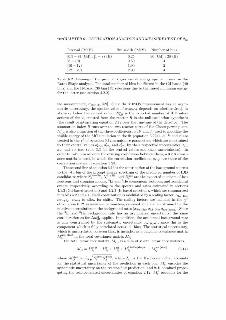
202CHAPTER 6. OSCILLATION ANALYSIS AND MEASUREMENT OF θ13
Interval ( MeV) Bin width ( MeV) Number of bins
[0.5− 8) (Gd) ; [1− 8) (H) 0.25 30 (Gd) ; 28 (H)[8− 10) 0.50 4[10− 12) 1.00 2[12− 20) 2.00 4
Table 6.2: Binning of the prompt trigger visible energy spectrum used in theRate+Shape analysis. The total number of bins is different in the Gd-based (40bins) and the H-based (38 bins) νe selections due to the raised minimum energyfor the latter (see section 4.2.2).
the measurement, σMINOS [59]. Since the MINOS measurement has an asym-metric uncertainty, the specific value of σMINOS depends on whether ∆m2
31 isabove or below the central value. Nν
i,R is the expected number of IBD inter-actions of the νe emitted from the reactor R in the null-oscillation hypothesis(the result of integrating equation 2.12 over the run-time of the detector). Thesummation index R runs over the two reactor cores of the Chooz power plant.Nνi,R is also a function of the three coefficients, a′, b′ and c′, used to modelize the
visible energy of the MC simulation in the fit (equation 3.22a). a′, b′ and c′ aretreated in the χ2 of equation 6.12 as nuisance parameters, which are constrainedto their central values a′CV, b′CV and c′CV by their respective uncertainties σa′ ,σb′ and σc′ (see table 3.3 for the central values and their uncertainties). Inorder to take into account the existing correlation between them, a 3×3 covari-ance matrix is used, in which the correlation coefficients ρx′y′ are those of thecorrelation matrix in equation 3.23.
The second line of equation 6.13 is the contribution of the background sourcesto the i-th bin of the prompt energy spectrum of the predicted number of IBDcandidates; where NFn+Sµ
i , NLi+Hei , and Nacc
i are the expected numbers of fastneutrons and stopping muons, 9Li and 8He cosmogenic isotopes, and accidentalevents, respectively, according to the spectra and rates estimated in sections4.1.3 (Gd-based selection) and 4.2.3 (H-based selection), which are summarizedin tables 4.2 and 4.4. Each contribution is modulated by a scaling factor, αLi+He,αFn+Sµ, αacc, to allow for shifts. The scaling factors are included in the χ2
of equation 6.12 as nuisance parameters, centered at 1 and constrained by therelative uncertainties on the background rates (σFn+Sµ, σLi+He, σacc(syst)). Sincethe 9Li and 8He background rate has an asymmetric uncertainty, the sameconsideration as for ∆m2
31 applies. In addition, the accidental background rateis only constrained by the systematic uncertainty σacc(syst), since this is thecomponent which is fully correlated across all bins. The statistical uncertainty,which is uncorrelated between bins, is included as a diagonal covariance matrixM
acc(stat)ij in the total covariance matrix Mij .The total covariance matrix, Mij , is a sum of several covariance matrices,
Mij = M statij +M r
ij +Mdij +M
Li+He(shape)ij +M
acc(stat)ij , (6.14)
where M statij = δij
√Npredi Npred
j , where δij is the Kronecker delta, accountsfor the statistical uncertainty of the prediction in each bin. M r
ij encodes thesystematic uncertainty on the reactor-flux prediction, and it is obtained propa-gating the reactor-related uncertainties of equation 2.12. Md
ij accounts for the
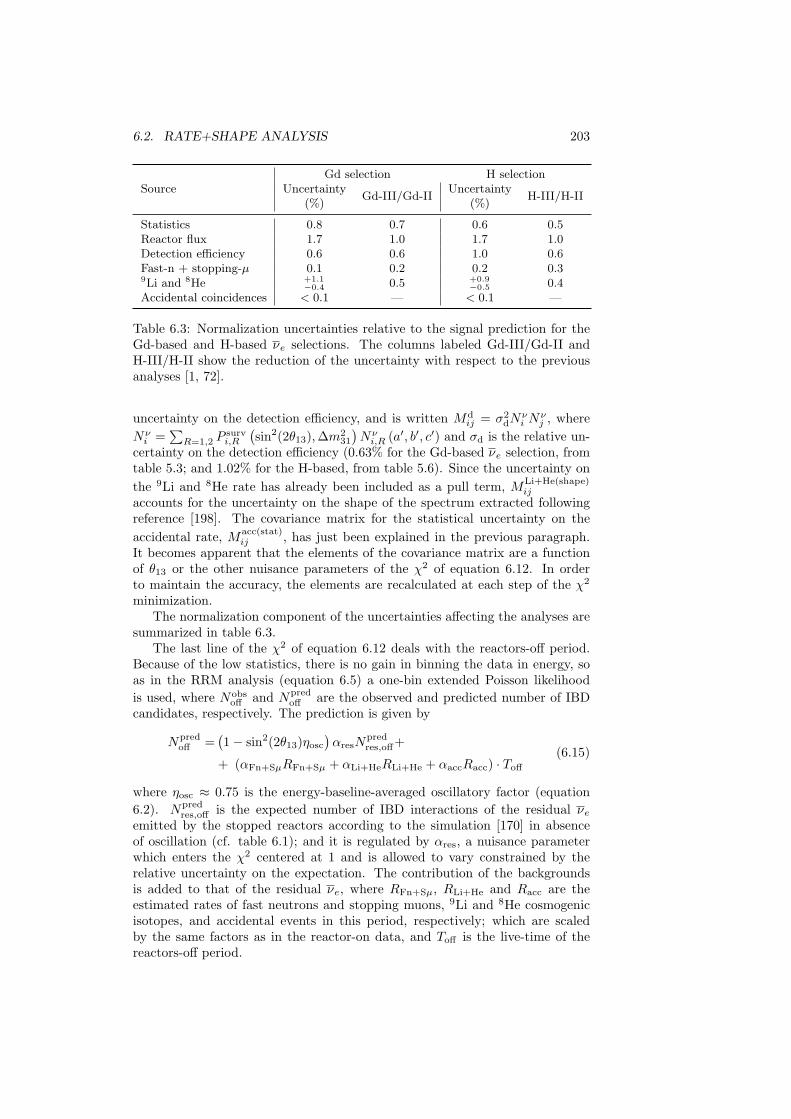
6.2. RATE+SHAPE ANALYSIS 203
SourceGd selection H selection
UncertaintyGd-III/Gd-II
UncertaintyH-III/H-II
(%) (%)
Statistics 0.8 0.7 0.6 0.5Reactor flux 1.7 1.0 1.7 1.0Detection efficiency 0.6 0.6 1.0 0.6Fast-n + stopping-µ 0.1 0.2 0.2 0.39Li and 8He +1.1
−0.4 0.5 +0.9−0.5 0.4
Accidental coincidences < 0.1 — < 0.1 —
Table 6.3: Normalization uncertainties relative to the signal prediction for theGd-based and H-based νe selections. The columns labeled Gd-III/Gd-II andH-III/H-II show the reduction of the uncertainty with respect to the previousanalyses [1, 72].
uncertainty on the detection efficiency, and is written Mdij = σ2
dNνi N
νj , where
Nνi =
∑R=1,2 P
survi,R
(sin2(2θ13),∆m2
31
)Nνi,R (a′, b′, c′) and σd is the relative un-
certainty on the detection efficiency (0.63% for the Gd-based νe selection, fromtable 5.3; and 1.02% for the H-based, from table 5.6). Since the uncertainty onthe 9Li and 8He rate has already been included as a pull term, MLi+He(shape)
ij
accounts for the uncertainty on the shape of the spectrum extracted followingreference [198]. The covariance matrix for the statistical uncertainty on theaccidental rate, Macc(stat)
ij , has just been explained in the previous paragraph.It becomes apparent that the elements of the covariance matrix are a functionof θ13 or the other nuisance parameters of the χ2 of equation 6.12. In orderto maintain the accuracy, the elements are recalculated at each step of the χ2
minimization.The normalization component of the uncertainties affecting the analyses are
summarized in table 6.3.The last line of the χ2 of equation 6.12 deals with the reactors-off period.
Because of the low statistics, there is no gain in binning the data in energy, soas in the RRM analysis (equation 6.5) a one-bin extended Poisson likelihoodis used, where Nobs
off and Npredoff are the observed and predicted number of IBD
candidates, respectively. The prediction is given by
Npredoff =
(1− sin2(2θ13)ηosc
)αresN
predres,off+
+ (αFn+SµRFn+Sµ + αLi+HeRLi+He + αaccRacc) · Toff
(6.15)
where ηosc ≈ 0.75 is the energy-baseline-averaged oscillatory factor (equation6.2). Npred
res,off is the expected number of IBD interactions of the residual νeemitted by the stopped reactors according to the simulation [170] in absenceof oscillation (cf. table 6.1); and it is regulated by αres, a nuisance parameterwhich enters the χ2 centered at 1 and is allowed to vary constrained by therelative uncertainty on the expectation. The contribution of the backgroundsis added to that of the residual νe, where RFn+Sµ, RLi+He and Racc are theestimated rates of fast neutrons and stopping muons, 9Li and 8He cosmogenicisotopes, and accidental events in this period, respectively; which are scaledby the same factors as in the reactor-on data, and Toff is the live-time of thereactors-off period.
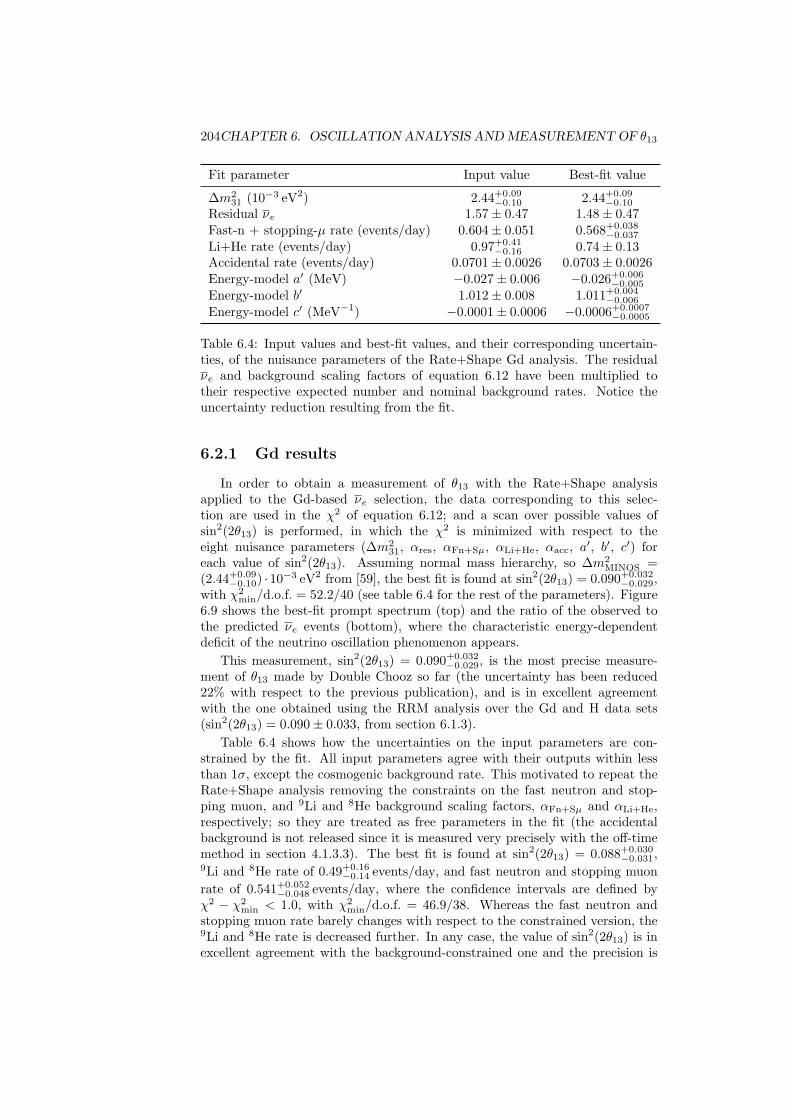
204CHAPTER 6. OSCILLATION ANALYSIS AND MEASUREMENT OF θ13
Fit parameter Input value Best-fit value
∆m231 (10−3 eV2) 2.44+0.09
−0.10 2.44+0.09−0.10
Residual νe 1.57± 0.47 1.48± 0.47Fast-n + stopping-µ rate (events/day) 0.604± 0.051 0.568+0.038
−0.037
Li+He rate (events/day) 0.97+0.41−0.16 0.74± 0.13
Accidental rate (events/day) 0.0701± 0.0026 0.0703± 0.0026Energy-model a′ (MeV) −0.027± 0.006 −0.026+0.006
−0.005
Energy-model b′ 1.012± 0.008 1.011+0.004−0.006
Energy-model c′ (MeV−1) −0.0001± 0.0006 −0.0006+0.0007−0.0005
Table 6.4: Input values and best-fit values, and their corresponding uncertain-ties, of the nuisance parameters of the Rate+Shape Gd analysis. The residualνe and background scaling factors of equation 6.12 have been multiplied totheir respective expected number and nominal background rates. Notice theuncertainty reduction resulting from the fit.
6.2.1 Gd results
In order to obtain a measurement of θ13 with the Rate+Shape analysisapplied to the Gd-based νe selection, the data corresponding to this selec-tion are used in the χ2 of equation 6.12; and a scan over possible values ofsin2(2θ13) is performed, in which the χ2 is minimized with respect to theeight nuisance parameters (∆m2
31, αres, αFn+Sµ, αLi+He, αacc, a′, b′, c′) foreach value of sin2(2θ13). Assuming normal mass hierarchy, so ∆m2
MINOS =(2.44+0.09
−0.10) ·10−3 eV2 from [59], the best fit is found at sin2(2θ13) = 0.090+0.032−0.029,
with χ2min/d.o.f. = 52.2/40 (see table 6.4 for the rest of the parameters). Figure
6.9 shows the best-fit prompt spectrum (top) and the ratio of the observed tothe predicted νe events (bottom), where the characteristic energy-dependentdeficit of the neutrino oscillation phenomenon appears.
This measurement, sin2(2θ13) = 0.090+0.032−0.029, is the most precise measure-
ment of θ13 made by Double Chooz so far (the uncertainty has been reduced22% with respect to the previous publication), and is in excellent agreementwith the one obtained using the RRM analysis over the Gd and H data sets(sin2(2θ13) = 0.090± 0.033, from section 6.1.3).
Table 6.4 shows how the uncertainties on the input parameters are con-strained by the fit. All input parameters agree with their outputs within lessthan 1σ, except the cosmogenic background rate. This motivated to repeat theRate+Shape analysis removing the constraints on the fast neutron and stop-ping muon, and 9Li and 8He background scaling factors, αFn+Sµ and αLi+He,respectively; so they are treated as free parameters in the fit (the accidentalbackground is not released since it is measured very precisely with the off-timemethod in section 4.1.3.3). The best fit is found at sin2(2θ13) = 0.088+0.030
−0.031,9Li and 8He rate of 0.49+0.16
−0.14 events/day, and fast neutron and stopping muonrate of 0.541+0.052
−0.048 events/day, where the confidence intervals are defined byχ2 − χ2
min < 1.0, with χ2min/d.o.f. = 46.9/38. Whereas the fast neutron and
stopping muon rate barely changes with respect to the constrained version, the9Li and 8He rate is decreased further. In any case, the value of sin2(2θ13) is inexcellent agreement with the background-constrained one and the precision is
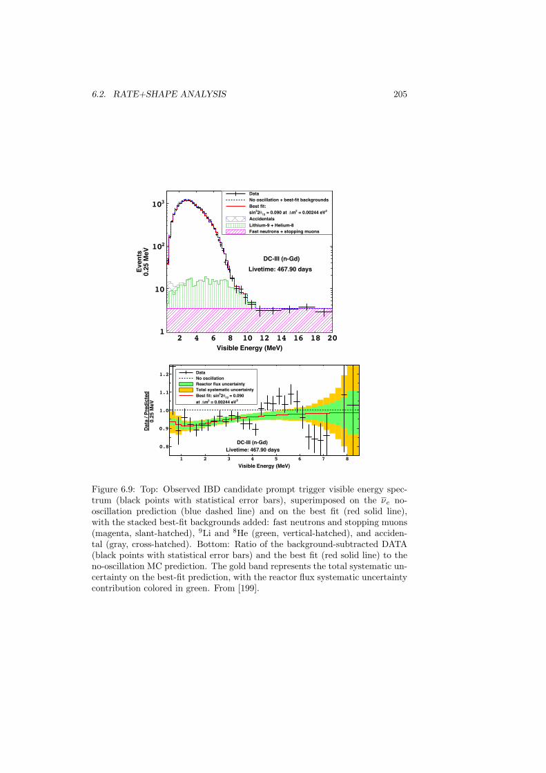
6.2. RATE+SHAPE ANALYSIS 205
Visible Energy (MeV)2 4 6 8 10 12 14 16 18 20
0.25
MeV
Even
ts
1
10
210
310DataNo oscillation + best-fit backgroundsBest fit:
2 = 0.00244 eV2m6 = 0.090 at 13e22sinAccidentalsLithium-9 + Helium-8Fast neutrons + stopping muons
DC-III (n-Gd)Livetime: 467.90 days
Visible Energy (MeV)1 2 3 4 5 6 7 8
0.
25 M
eVD
ata
/ Pre
dict
ed
0.8
0.9
1.0
1.1
1.2 DataNo oscillationReactor flux uncertaintyTotal systematic uncertainty
= 0.09013e22Best fit: sin2 = 0.00244 eV2m6at
DC-III (n-Gd)Livetime: 467.90 days
Figure 6.9: Top: Observed IBD candidate prompt trigger visible energy spec-trum (black points with statistical error bars), superimposed on the νe no-oscillation prediction (blue dashed line) and on the best fit (red solid line),with the stacked best-fit backgrounds added: fast neutrons and stopping muons(magenta, slant-hatched), 9Li and 8He (green, vertical-hatched), and acciden-tal (gray, cross-hatched). Bottom: Ratio of the background-subtracted DATA(black points with statistical error bars) and the best fit (red solid line) to theno-oscillation MC prediction. The gold band represents the total systematic un-certainty on the best-fit prediction, with the reactor flux systematic uncertaintycontribution colored in green. From [199].
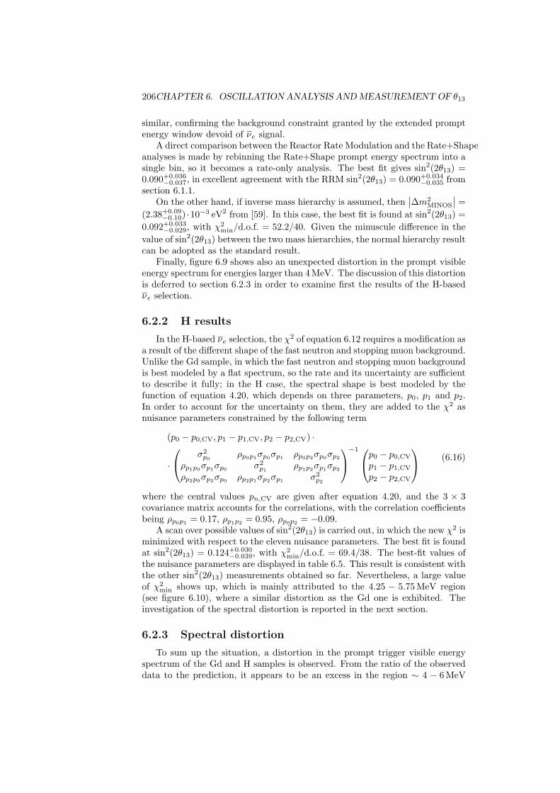
206CHAPTER 6. OSCILLATION ANALYSIS AND MEASUREMENT OF θ13
similar, confirming the background constraint granted by the extended promptenergy window devoid of νe signal.
A direct comparison between the Reactor Rate Modulation and the Rate+Shapeanalyses is made by rebinning the Rate+Shape prompt energy spectrum into asingle bin, so it becomes a rate-only analysis. The best fit gives sin2(2θ13) =0.090+0.036
−0.037, in excellent agreement with the RRM sin2(2θ13) = 0.090+0.034−0.035 from
section 6.1.1.On the other hand, if inverse mass hierarchy is assumed, then
∣∣∆m2MINOS
∣∣ =(2.38+0.09
−0.10) ·10−3 eV2 from [59]. In this case, the best fit is found at sin2(2θ13) =0.092+0.033
−0.029, with χ2min/d.o.f. = 52.2/40. Given the minuscule difference in the
value of sin2(2θ13) between the two mass hierarchies, the normal hierarchy resultcan be adopted as the standard result.
Finally, figure 6.9 shows also an unexpected distortion in the prompt visibleenergy spectrum for energies larger than 4 MeV. The discussion of this distortionis deferred to section 6.2.3 in order to examine first the results of the H-basedνe selection.
6.2.2 H results
In the H-based νe selection, the χ2 of equation 6.12 requires a modification asa result of the different shape of the fast neutron and stopping muon background.Unlike the Gd sample, in which the fast neutron and stopping muon backgroundis best modeled by a flat spectrum, so the rate and its uncertainty are sufficientto describe it fully; in the H case, the spectral shape is best modeled by thefunction of equation 4.20, which depends on three parameters, p0, p1 and p2.In order to account for the uncertainty on them, they are added to the χ2 asnuisance parameters constrained by the following term
(p0 − p0,CV, p1 − p1,CV, p2 − p2,CV) ·
·
σ2p0 ρp0p1σp0σp1 ρp0p2σp0σp2
ρp1p0σp1σp0 σ2p1 ρp1p2σp1σp2
ρp2p0σp2σp0 ρp2p1σp2σp1 σ2p2
−1p0 − p0,CV
p1 − p1,CV
p2 − p2,CV
(6.16)
where the central values pn,CV are given after equation 4.20, and the 3 × 3covariance matrix accounts for the correlations, with the correlation coefficientsbeing ρp0p1 = 0.17, ρp1p2 = 0.95, ρp0p2 = −0.09.
A scan over possible values of sin2(2θ13) is carried out, in which the new χ2 isminimized with respect to the eleven nuisance parameters. The best fit is foundat sin2(2θ13) = 0.124+0.030
−0.039, with χ2min/d.o.f. = 69.4/38. The best-fit values of
the nuisance parameters are displayed in table 6.5. This result is consistent withthe other sin2(2θ13) measurements obtained so far. Nevertheless, a large valueof χ2
min shows up, which is mainly attributed to the 4.25 − 5.75 MeV region(see figure 6.10), where a similar distortion as the Gd one is exhibited. Theinvestigation of the spectral distortion is reported in the next section.
6.2.3 Spectral distortion
To sum up the situation, a distortion in the prompt trigger visible energyspectrum of the Gd and H samples is observed. From the ratio of the observeddata to the prediction, it appears to be an excess in the region ∼ 4 − 6 MeV
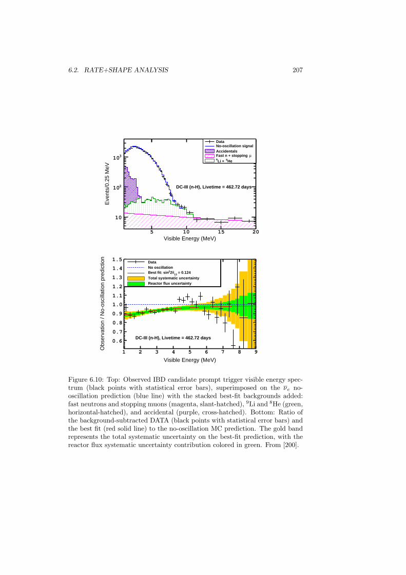
6.2. RATE+SHAPE ANALYSIS 207
Visible Energy (MeV)5 10 15 20
Eve
nts/
0.25
MeV
10
210
310
DC-III (n-H), Livetime = 462.72 days
DataNo-oscillation signalAccidentals
µFast n + stopping He8Li + 9
Visible Energy (MeV)
1 2 3 4 5 6 7 8 9
Obs
erva
tion
/ No-
osci
llatio
n pr
edic
tion
0.6
0.7
0.8
0.9
1.0
1.1
1.2
1.3
1.4
1.5
DC-III (n-H), Livetime = 462.72 days
DataNo oscillation
= 0.12413
θ22Best fit: sinTotal systematic uncertaintyReactor flux uncertainty
Figure 6.10: Top: Observed IBD candidate prompt trigger visible energy spec-trum (black points with statistical error bars), superimposed on the νe no-oscillation prediction (blue line) with the stacked best-fit backgrounds added:fast neutrons and stopping muons (magenta, slant-hatched), 9Li and 8He (green,horizontal-hatched), and accidental (purple, cross-hatched). Bottom: Ratio ofthe background-subtracted DATA (black points with statistical error bars) andthe best fit (red solid line) to the no-oscillation MC prediction. The gold bandrepresents the total systematic uncertainty on the best-fit prediction, with thereactor flux systematic uncertainty contribution colored in green. From [200].
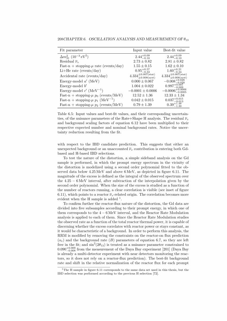
208CHAPTER 6. OSCILLATION ANALYSIS AND MEASUREMENT OF θ13
Fit parameter Input value Best-fit value
∆m231 (10−3 eV2) 2.44+0.09
−0.10 2.44+0.09−0.10
Residual νe 2.73± 0.82 2.81± 0.82Fast-n + stopping-µ rate (events/day) 1.55± 0.15 1.62± 0.10Li+He rate (events/day) 0.95+0.57
−0.33 1.60+0.21−0.24
Accidental rate (events/day) 4.334±0.007(stat)±0.008(syst) 4.334±0.007(stat)
±0.008(syst)
Energy-model a′ (MeV) 0.000± 0.067 −0.008+0.028−0.020
Energy-model b′ 1.004± 0.022 0.997+0.007−0.009
Energy-model c′ (MeV−1) −0.0001± 0.0006 −0.0006+0.0006−0.0005
Fast-n + stopping-µ p0 (events/MeV) 12.52± 1.36 12.33± 1.34Fast-n + stopping-µ p1 (MeV−1) 0.042± 0.015 0.037+0.015
−0.013
Fast-n + stopping-µ p2 (events/MeV) 0.79± 1.39 0.39+1.48−1.30
Table 6.5: Input values and best-fit values, and their corresponding uncertain-ties, of the nuisance parameters of the Rate+Shape H analysis. The residual νeand background scaling factors of equation 6.12 have been multiplied to theirrespective expected number and nominal background rates. Notice the uncer-tainty reduction resulting from the fit.
with respect to the IBD candidate prediction. This suggests that either anunexpected background or an unaccounted νe contribution is entering both Gd-based and H-based IBD selections.
To test the nature of the distortion, a simple sideband analysis on the Gdsample is performed, in which the prompt energy spectrum in the vicinity ofthe distortion is modelized using a second order polynomial fitted to the ob-served data below 4.25 MeV and above 6 MeV, as depicted in figure 6.11. Themagnitude of the excess is defined as the integral of the observed spectrum overthe 4.25 − 6 MeV interval, after subtraction of the interpolation given by thesecond order polynomial. When the size of the excess is studied as a function ofthe number of reactors running, a clear correlation is visible (see inset of figure6.11), which points to a reactor νe-related origin. The correlation becomes moreevident when the H sample is added 1.
To confirm further the reactor-flux nature of the distortion, the Gd data aredivided into five subsamples according to their prompt energy, in which one ofthem corresponds to the 4− 6 MeV interval, and the Reactor Rate Modulationanalysis is applied to each of them. Since the Reactor Rate Modulation studiesthe observed rate as a function of the total reactor thermal power, it is capable ofdiscerning whether the excess correlates with reactor power or stays constant, asit would be characteristic of a background. In order to perform this analysis, theRRM is modified by removing the constraints on the reactor-on flux prediction(αr) and the background rate (B) parameters of equation 6.7, so they are leftfree in the fit; and sin2(2θ13) is treated as a nuisance parameter constrained to0.090+0.009
−0.008 from the measurement of the Daya Bay experiment [201] (Daya Bayis already a multi-detector experiment with near detectors monitoring the reac-tors, so it does not rely on a reactor-flux prediction). The best-fit backgroundrate and shift in the relative normalization of the reactor flux for each prompt
1The H sample in figure 6.11 corresponds to the same data set used in this thesis, but theIBD selection was performed according to the previous H selection [72].
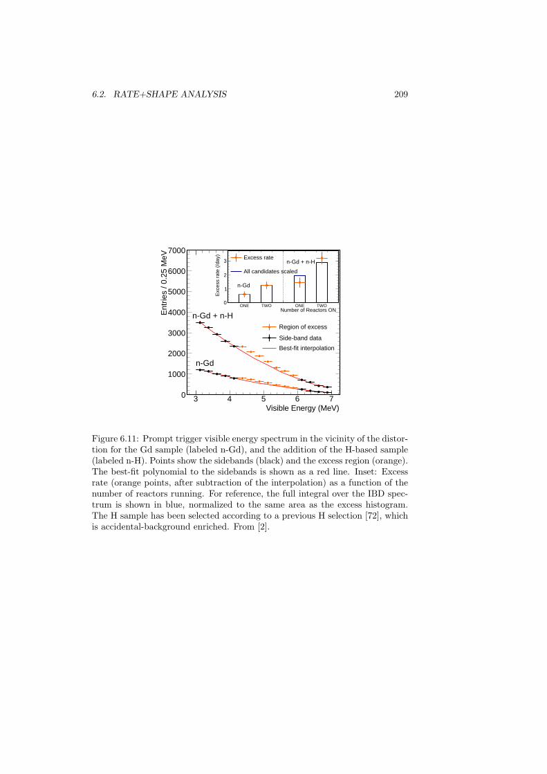
6.2. RATE+SHAPE ANALYSIS 209
Visible Energy (MeV)3 4 5 6 7
Ent
ries
/ 0.2
5 M
eV
0
1000
2000
3000
4000
5000
6000
7000
n-Gd
n-Gd + n-HRegion of excess
Side-band data
Best-fit interpolation
Number of Reactors ON ONE TWO ONE TWO
Exc
ess
rate
(/d
ay)
0
1
2
3Excess rate
All candidates scaled
n-Gd
n-Gd + n-H
Figure 6.11: Prompt trigger visible energy spectrum in the vicinity of the distor-tion for the Gd sample (labeled n-Gd), and the addition of the H-based sample(labeled n-H). Points show the sidebands (black) and the excess region (orange).The best-fit polynomial to the sidebands is shown as a red line. Inset: Excessrate (orange points, after subtraction of the interpolation) as a function of thenumber of reactors running. For reference, the full integral over the IBD spec-trum is shown in blue, normalized to the same area as the excess histogram.The H sample has been selected according to a previous H selection [72], whichis accidental-background enriched. From [2].
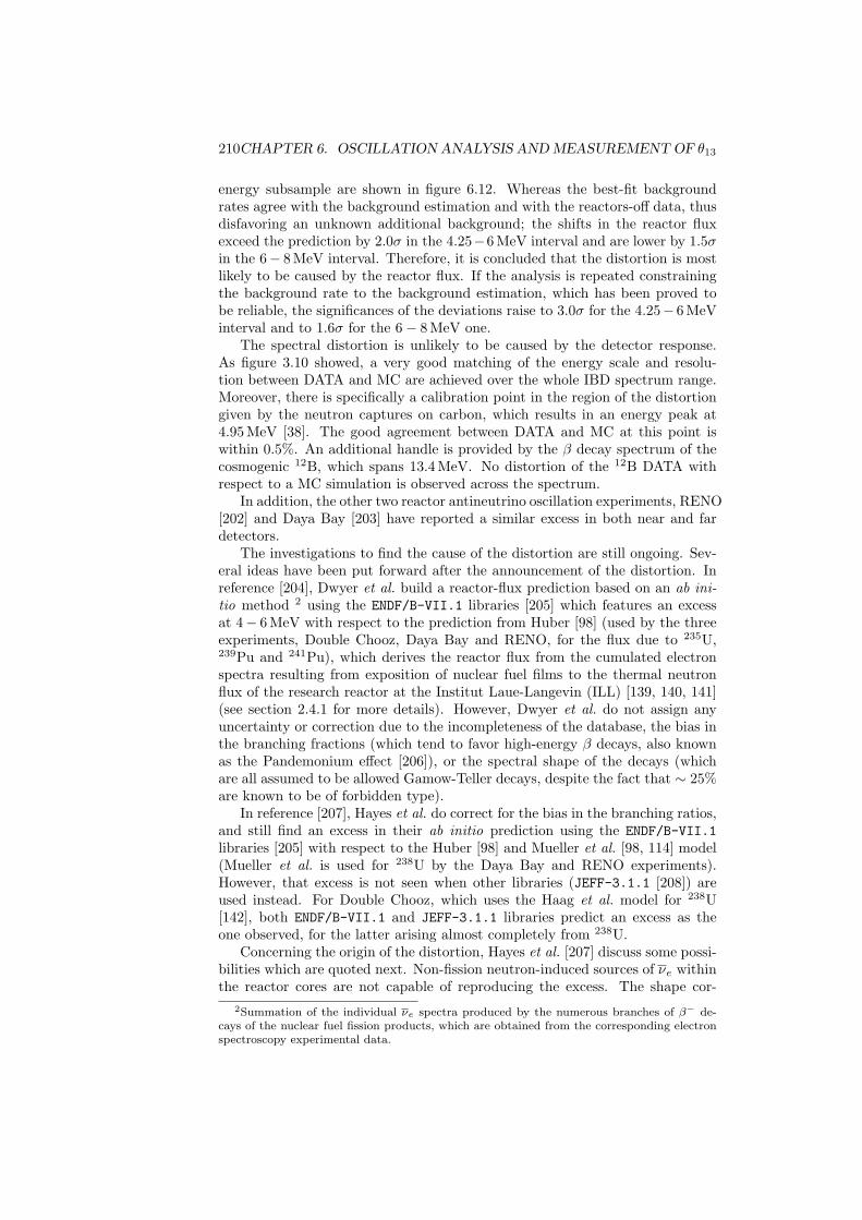
210CHAPTER 6. OSCILLATION ANALYSIS AND MEASUREMENT OF θ13
energy subsample are shown in figure 6.12. Whereas the best-fit backgroundrates agree with the background estimation and with the reactors-off data, thusdisfavoring an unknown additional background; the shifts in the reactor fluxexceed the prediction by 2.0σ in the 4.25−6 MeV interval and are lower by 1.5σin the 6− 8 MeV interval. Therefore, it is concluded that the distortion is mostlikely to be caused by the reactor flux. If the analysis is repeated constrainingthe background rate to the background estimation, which has been proved tobe reliable, the significances of the deviations raise to 3.0σ for the 4.25− 6 MeVinterval and to 1.6σ for the 6− 8 MeV one.
The spectral distortion is unlikely to be caused by the detector response.As figure 3.10 showed, a very good matching of the energy scale and resolu-tion between DATA and MC are achieved over the whole IBD spectrum range.Moreover, there is specifically a calibration point in the region of the distortiongiven by the neutron captures on carbon, which results in an energy peak at4.95 MeV [38]. The good agreement between DATA and MC at this point iswithin 0.5%. An additional handle is provided by the β decay spectrum of thecosmogenic 12B, which spans 13.4 MeV. No distortion of the 12B DATA withrespect to a MC simulation is observed across the spectrum.
In addition, the other two reactor antineutrino oscillation experiments, RENO[202] and Daya Bay [203] have reported a similar excess in both near and fardetectors.
The investigations to find the cause of the distortion are still ongoing. Sev-eral ideas have been put forward after the announcement of the distortion. Inreference [204], Dwyer et al. build a reactor-flux prediction based on an ab ini-tio method 2 using the ENDF/B-VII.1 libraries [205] which features an excessat 4− 6 MeV with respect to the prediction from Huber [98] (used by the threeexperiments, Double Chooz, Daya Bay and RENO, for the flux due to 235U,239Pu and 241Pu), which derives the reactor flux from the cumulated electronspectra resulting from exposition of nuclear fuel films to the thermal neutronflux of the research reactor at the Institut Laue-Langevin (ILL) [139, 140, 141](see section 2.4.1 for more details). However, Dwyer et al. do not assign anyuncertainty or correction due to the incompleteness of the database, the bias inthe branching fractions (which tend to favor high-energy β decays, also knownas the Pandemonium effect [206]), or the spectral shape of the decays (whichare all assumed to be allowed Gamow-Teller decays, despite the fact that ∼ 25%are known to be of forbidden type).
In reference [207], Hayes et al. do correct for the bias in the branching ratios,and still find an excess in their ab initio prediction using the ENDF/B-VII.1libraries [205] with respect to the Huber [98] and Mueller et al. [98, 114] model(Mueller et al. is used for 238U by the Daya Bay and RENO experiments).However, that excess is not seen when other libraries (JEFF-3.1.1 [208]) areused instead. For Double Chooz, which uses the Haag et al. model for 238U[142], both ENDF/B-VII.1 and JEFF-3.1.1 libraries predict an excess as theone observed, for the latter arising almost completely from 238U.
Concerning the origin of the distortion, Hayes et al. [207] discuss some possi-bilities which are quoted next. Non-fission neutron-induced sources of νe withinthe reactor cores are not capable of reproducing the excess. The shape cor-
2Summation of the individual νe spectra produced by the numerous branches of β− de-cays of the nuclear fuel fission products, which are obtained from the corresponding electronspectroscopy experimental data.
6.2. RATE+SHAPE ANALYSIS 211
Visible Energy (MeV)0 5 10 15 20
)-1
MeV
-1B
ackg
roun
d R
ate
(day
-0.2
0.0
0.2
0.4
0.6
0.8
BG estimation
Best-fit BG
2-Off observation
Visible Energy (MeV)0 1 2 3 4 5 6 7 8
(%
)Φ∆
Flu
x no
rmal
izat
ion
-30
-20
-10
0
10
20
Φ∆Best-fit
(BG constrained)Φ∆Best-fit
uncertaintyΦ
Figure 6.12: Modified Reactor Rate Modulation analysis (see text for the de-tails) applied to subsamples of the Gd-based νe selection according to theirprompt energy. Top: Best-fit background rates (black circles with error boxes)for each subsample. For comparison purposes, the background rate estimationis shown as a line and its uncertainty as a yellow band, and the reactors-off ob-served data are represented by blue empty triangles with statistical error bars.Bottom: Best-fit shifts of the reactor-flux normalization with respect to theprediction, with the background rate left free (black circles with error boxes)and with the background constrained to the estimation (red empty squares witherror bars). The uncertainty on the reactor-flux prediction is shown as a yellowband. The analysis is restricted to the νe-dominated region (below 8 MeV).From [2].
212CHAPTER 6. OSCILLATION ANALYSIS AND MEASUREMENT OF θ13
rections from a proper treatment of the forbidden decays cannot explain themagnitude of the excess either. The role of 238U is examined, since its contri-bution in the 4 − 6 MeV region is twice that of 235U. Both ENDF/B-VII.1 andJEFF-3.1.1 libraries predict a shoulder in the 238U spectrum with respect toMueller et al. [114], but to reproduce the size exclusively with 238U would requirefission yields a factor four and two larger than those of the libraries, respectively.For Haag et al. [142], the shoulder from 238U in JEFF-3.1.1 may explain theexcess, but more data is needed before such conclusion can be drawn. Anotherpossibility is that pressurized water reactors (PWR), like those in the DoubleChooz, Daya Bay and RENO experiments, are known to have a harder neutronspectrum, with a more sizable epithermal component, than the research reactorat the ILL where the reference cumulated electron spectra for 235U, 239Pu and241Pu used by the three experiments were measured. This difference in the neu-tron energies may alter the fission yields, enhancing certain nuclei and buildingthe excess. Finally, a possible error in the original ILL measurements cannot beexcluded.
Regarding the impact of the spectral distortion to the Rate+Shape mea-surements of θ13, it must be noted first that almost all the oscillation signatureis concentrated at prompt energies below 4 MeV, where the observed data ex-hibits the characteristic energy-dependent deficit (cf. the ratio plots in figures6.9 and 6.10), so an unaccounted structure above 4 MeV has little effect on thedetermination of θ13. This was tested explicitly by including an artificial excessin the predicted IBD candidate spectrum in the region of the distortion, whosenormalization was left free in the fit. After trying multiple peak energies andwidths, none resulted in a deviation of θ13 larger than 30% of its uncertaintyinterval, demonstrating that the distortion does not affect significantly the θ13
measurement. Another proof of the robustness of the Double Chooz measure-ments is the agreement found between the Rate+Shape results and the ReactorRate Modulation ones, the latter not being sensitive to the distortion.
However, the appearance of a distortion in the observed spectrum not antic-ipated by the reactor-flux model casts doubts on the accuracy of the predictionand the quoted uncertainty. Consequently, there is nothing to be gained froma simultaneous Rate+Shape analysis of the Gd-based and H-based νe samplesto decrease the uncertainty on θ13. Notice that this conclusion does not af-fect so severely the Reactor Rate Modulation analysis, which does not use thespectrum shape but the total integral, which is anchored to a short-baselinemeasurement by the Bugey4 experiment (see equation 2.11). In any case, thisreinforces the necessity of having a near detector close to the reactor cores, inorder to reduce the dependence on a reactor model and to improve the precisionof the measurement of θ13. This is precisely the subject of the next section.
6.3 Two-detector outlook
To conclude the chapter, the expected precision on θ13 resulting from theanalysis of the data from the Near and Far Detectors is discussed. The NearDetector became operative during the writing of this thesis, and no oscillationanalysis has been performed yet using the Near Detector DATA. Therefore, thefollowing study utilizes only the νe MC simulation developed for the Far Detec-tor as a proxy for the observed and expected νe interactions in both detectors.
6.3. TWO-DETECTOR OUTLOOK 213
An oscillation corresponding to sin2(2θ13) = 0.10 is artificially induced in theobserved sample.
The oscillation analysis chosen is the Rate+Shape analysis, since it has pro-vided the most precise θ13 measurements so far. The χ2 statistic used is similarto that of equation 6.12, although it has been extended to accommodate twodetectors:
χ2 =∑i
∑j
(Npredi −Nobs
i
)M−1ij
(Npredj −Nobs
j
)+
+(
∆m231 −∆m2
MINOS
σMINOS
)2
+
+∑
D=ND, FD
(αDFn+Sµ − 1σDFn+Sµ
)2
+
(αDLi+He − 1σDLi+He
)2
+
(αDacc − 1σDacc(syst)
)2
(6.17)where the sum in i and j is over the bins in which the prompt spectra of thetwo detectors have been divided (following the same convention as in table 6.2).The Far and Near Detector prompt spectra can be regarded as two vectors,~NFD and ~NND, respectively; which are concatenated to form a single vector, so∑
i
∑j
(Npredi −Nobs
i
)M−1ij
(Npredj −Nobs
j
)=
=(~NFD,pred − ~NFD,obs, ~NND,pred − ~NND,obs
)·
·(MFD M corr
M corr MND
)−1( ~NFD,pred − ~NFD,obs
~NND,pred − ~NND,obs
) (6.18)
where the covariance matrix, M , which accounts for the uncertainties describedlater, has been divided into four blocks. The diagonal blocks account for theuncertainties affecting a single detector, MFD for the Far Detector and MND
for the Near Detector. The off-diagonal blocks account for the correlated un-certainties between detectors. The internal structure of each block depends onthe correlations between the energy bins which are relating.
The observed (Nobsi ) and predicted (Npred
i ) number of IBD candidates inthe i-th bin are obtained using the Gd selection (section 4.1). In this case,the predicted number of IBD candidates in the i-th bin of the D-th detector isexpressed as
ND,predi =
∑R=1,2
P surv,Di,R
(sin2(2θ13),∆m2
31
)Nν,Di,R (b′) +
+ αDFn+SµNFn+Sµi + αDLi+HeN
Li+Hei + αDaccN
acci ,
(6.19)
where P surv,Di,R
(sin2(2θ13),∆m2
31
)is the survival probability of the νe emitted
from the reactor R which interacted in the detector D and ended up in the i-thenergy bin, which is a function of sin2(2θ13) and ∆m2
31 (as in equation 1.54).The treatment of ∆m2
31 is identical to the one-detector fit, and normal masshierarchy is assumed, so ∆m2
MINOS = (2.44+0.09−0.10) · 10−3 eV2 from reference [59].
Nν,Di,R is the expected number of νe IBD interactions in the detector D coming
from the reactor R in the null-oscillation hypothesis. Since a MC prediction has
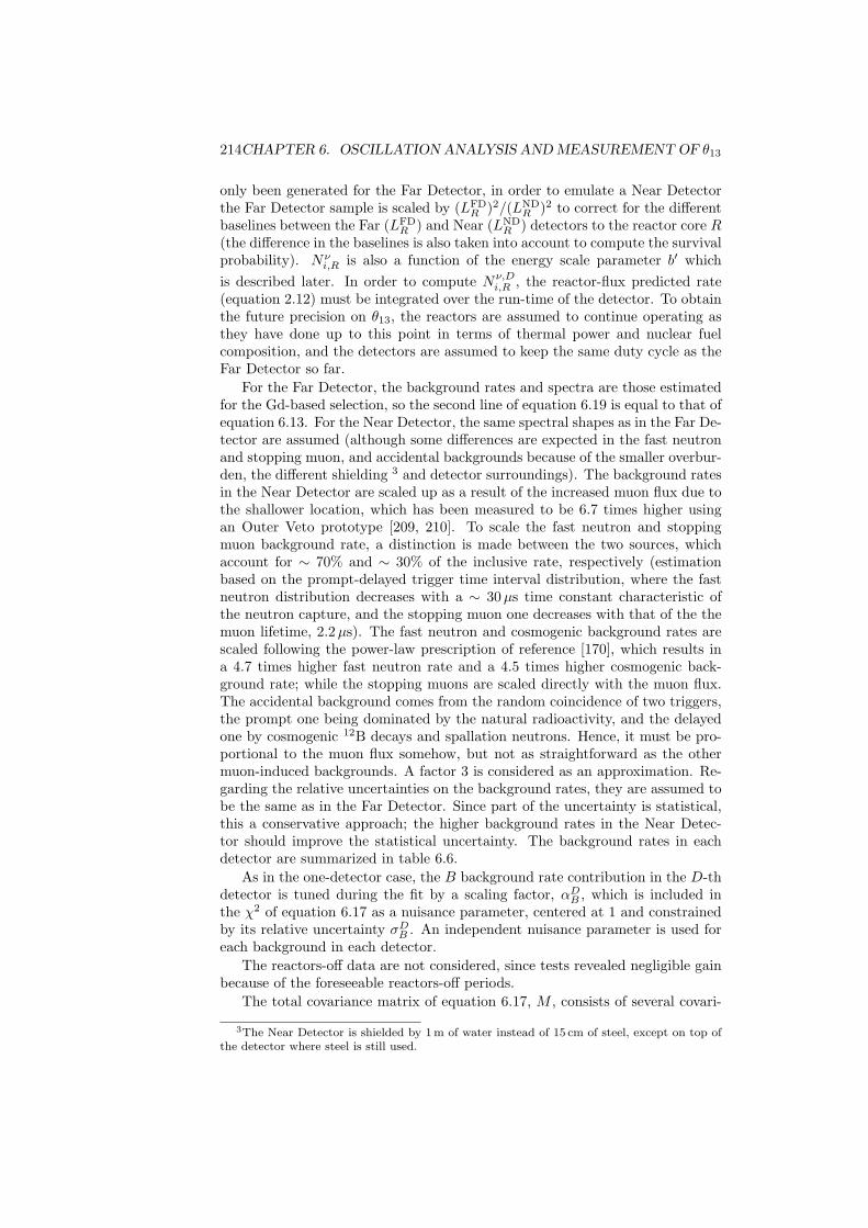
214CHAPTER 6. OSCILLATION ANALYSIS AND MEASUREMENT OF θ13
only been generated for the Far Detector, in order to emulate a Near Detectorthe Far Detector sample is scaled by (LFD
R )2/(LNDR )2 to correct for the different
baselines between the Far (LFDR ) and Near (LND
R ) detectors to the reactor core R(the difference in the baselines is also taken into account to compute the survivalprobability). Nν
i,R is also a function of the energy scale parameter b′ whichis described later. In order to compute Nν,D
i,R , the reactor-flux predicted rate(equation 2.12) must be integrated over the run-time of the detector. To obtainthe future precision on θ13, the reactors are assumed to continue operating asthey have done up to this point in terms of thermal power and nuclear fuelcomposition, and the detectors are assumed to keep the same duty cycle as theFar Detector so far.
For the Far Detector, the background rates and spectra are those estimatedfor the Gd-based selection, so the second line of equation 6.19 is equal to that ofequation 6.13. For the Near Detector, the same spectral shapes as in the Far De-tector are assumed (although some differences are expected in the fast neutronand stopping muon, and accidental backgrounds because of the smaller overbur-den, the different shielding 3 and detector surroundings). The background ratesin the Near Detector are scaled up as a result of the increased muon flux due tothe shallower location, which has been measured to be 6.7 times higher usingan Outer Veto prototype [209, 210]. To scale the fast neutron and stoppingmuon background rate, a distinction is made between the two sources, whichaccount for ∼ 70% and ∼ 30% of the inclusive rate, respectively (estimationbased on the prompt-delayed trigger time interval distribution, where the fastneutron distribution decreases with a ∼ 30µs time constant characteristic ofthe neutron capture, and the stopping muon one decreases with that of the themuon lifetime, 2.2µs). The fast neutron and cosmogenic background rates arescaled following the power-law prescription of reference [170], which results ina 4.7 times higher fast neutron rate and a 4.5 times higher cosmogenic back-ground rate; while the stopping muons are scaled directly with the muon flux.The accidental background comes from the random coincidence of two triggers,the prompt one being dominated by the natural radioactivity, and the delayedone by cosmogenic 12B decays and spallation neutrons. Hence, it must be pro-portional to the muon flux somehow, but not as straightforward as the othermuon-induced backgrounds. A factor 3 is considered as an approximation. Re-garding the relative uncertainties on the background rates, they are assumed tobe the same as in the Far Detector. Since part of the uncertainty is statistical,this a conservative approach; the higher background rates in the Near Detec-tor should improve the statistical uncertainty. The background rates in eachdetector are summarized in table 6.6.
As in the one-detector case, the B background rate contribution in the D-thdetector is tuned during the fit by a scaling factor, αDB , which is included inthe χ2 of equation 6.17 as a nuisance parameter, centered at 1 and constrainedby its relative uncertainty σDB . An independent nuisance parameter is used foreach background in each detector.
The reactors-off data are not considered, since tests revealed negligible gainbecause of the foreseeable reactors-off periods.
The total covariance matrix of equation 6.17, M , consists of several covari-
3The Near Detector is shielded by 1 m of water instead of 15 cm of steel, except on top ofthe detector where steel is still used.
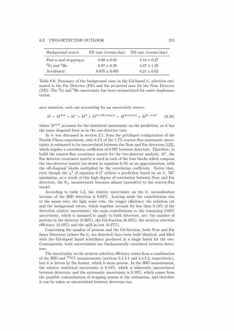
6.3. TWO-DETECTOR OUTLOOK 215
Background source FD rate (events/day) ND rate (events/day)
Fast-n and stopping-µ 0.60± 0.05 3.18± 0.279Li and 8He 0.97± 0.29 4.37± 1.29Accidental 0.070± 0.005 0.21± 0.02
Table 6.6: Summary of the background rates in the Gd-based νe selection esti-mated in the Far Detector (FD) and the projected ones for the Near Detector(ND). The 9Li and 8He uncertainty has been symmetrized for easier implemen-tation.
ance matrices, each one accounting for an uncertainty source:
M = M stat +M r +Md +MLi+He(shape) +Macc(stat) +ME−scale (6.20)
where M stat accounts for the statistical uncertainty on the prediction, so it hasthe same diagonal form as in the one-detector case.
As it was discussed in section 2.1, from the privileged configuration of theDouble Chooz experiment, only 0.1% of the 1.7% reactor-flux systematic uncer-tainty is estimated to be uncorrelated between the Near and Far detectors [122],which implies a correlation coefficient of 0.997 between detectors. Therefore, tobuild the reactor-flux covariance matrix for the two-detector analysis, M r, theFar detector covariance matrix is used in each of the four blocks which composethe two-detector matrix (as shown in equation 6.18) as an approximation, withthe off-diagonal blocks multiplied by the correlation coefficient. Notice that,even though the χ2 of equation 6.17 utilizes a prediction based on an νe MCsimulation, as a result of this high degree of correlation between Near and Fardetectors, the θ13 measurement becomes almost insensitive to the reactor-fluxmodel.
According to table 5.3, the relative uncertainty on the νe normalizationbecause of the IBD detection is 0.63%. Leaving aside the contributions dueto the muon veto, the light noise cuts, the trigger efficiency, the isolation cutand the background vetoes, which together account for less than 0.13% of thedetection relative uncertainty; the main contributions to the remaining 0.62%uncertainty, which is assumed to apply to both detectors, are: the number ofprotons in the detector (0.30%), the Gd-fraction (0.43%), the neutron selectionefficiency (0.19%) and the spill-in/out (0.27%).
Concerning the number of protons and the Gd-fraction, both Near and FarInner Detectors (where the νe are detected) have been built identical, and filledwith the Gd-doped liquid scintillator produced in a single batch for the two.Consequently, both uncertainties are fundamentally correlated between detec-tors.
The uncertainty on the neutron selection efficiency arises from a combinationof the IBD and 252Cf measurements (sections 5.4.2.1 and 5.4.2.2, respectively),but it is driven by the former, which is more precise. In the IBD measurement,the relative statistical uncertainty is 0.10%, which is inherently uncorrelatedbetween detectors; and the systematic uncertainty is 0.19%, which comes fromthe possible contamination of stopping muons in the estimation, and thereforeit can be taken as uncorrelated between detectors too.
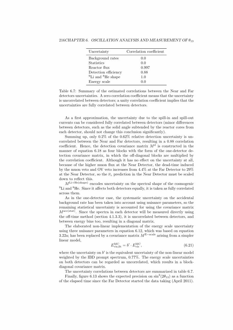
216CHAPTER 6. OSCILLATION ANALYSIS AND MEASUREMENT OF θ13
Uncertainty Correlation coefficient
Background rates 0.0Statistics 0.0Reactor flux 0.997Detection efficiency 0.889Li and 8He shape 1.0Energy scale 0.0
Table 6.7: Summary of the estimated correlations between the Near and Fardetectors uncertainties. A zero correlation coefficient means that the uncertaintyis uncorrelated between detectors; a unity correlation coefficient implies that theuncertainties are fully correlated between detectors.
As a first approximation, the uncertainty due to the spill-in and spill-outcurrents can be considered fully correlated between detectors (minor differencesbetween detectors, such as the solid angle subtended by the reactor cores fromeach detector, should not change this conclusion significantly).
Summing up, only 0.2% of the 0.62% relative detection uncertainty is un-correlated between the Near and Far detectors, resulting in a 0.88 correlationcoefficient. Hence, the detection covariance matrix Md is constructed in themanner of equation 6.18 as four blocks with the form of the one-detector de-tection covariance matrix, in which the off-diagonal blocks are multiplied bythe correlation coefficient. Although it has no effect on the uncertainty at all,because of the higher muon flux at the Near Detector, the dead-time inducedby the muon veto and OV veto increases from 4.4% at the Far Detector to 29%at the Near Detector, so the νe prediction in the Near Detector must be scaleddown to reflect this.
MLi+He(shape) encodes uncertainty on the spectral shape of the cosmogenic9Li and 8He. Since it affects both detectors equally, it is taken as fully correlatedacross them.
As in the one-detector case, the systematic uncertainty on the accidentalbackground rate has been taken into account using nuisance parameters, so theremaining statistical uncertainty is accounted for using the covariance matrixMacc(stat). Since the spectra in each detector will be measured directly usingthe off-time method (section 4.1.3.3), it is uncorrelated between detectors, andbetween energy bins too, resulting in a diagonal matrix.
The elaborated non-linear implementation of the energy scale uncertaintyusing three nuisance parameters in equation 6.12, which was based on equation3.22a; has been replaced by a covariance matrix ME−scale arising from a simplerlinear model,
EMCvis,fit = b′ · EMC
vis , (6.21)
where the uncertainty on b′ is the equivalent uncertainty of the non-linear modelweighted by the IBD prompt spectrum, 0.77%. The energy scale uncertaintieson both detectors can be regarded as uncorrelated, which results in a block-diagonal covariance matrix.
The uncertainty correlations between detectors are summarized in table 6.7.Finally, figure 6.13 shows the expected precision on sin2(2θ13) as a function
of the elapsed time since the Far Detector started the data taking (April 2011).
6.3. TWO-DETECTOR OUTLOOK 217
Total years of data-taking since April 20110 1 2 3 4 5 6 7 8
= 0
.113θ22
err
or o
n si
nσ
Exp
ecte
d 1
0.00
0.01
0.02
0.03
0.04
0.05
0.06
0.07DC-II (n-Gd): FD only
DC-II (n-Gd): ND and FD
DC-III (n-Gd): FD only
DC-III (n-Gd): ND and FD
Range of potential precision (n-Gd): ND and FD
Figure 6.13: Expected precision of the Double Chooz Rate+Shape measurementof sin2(2θ13) considering only IBD neutrons captured on Gd, as a function of theelapsed time since the Far Detector (FD) started the data taking (April 2011),assuming sin2(2θ13) = 0.10 (see text for further assumptions). The projectionsusing only the Far Detector (blue dashed line) and both Near Detector (ND)and Far Detector (blue solid line) are shown. The shaded region represents thepotential improvement brought by the reduction of systematic uncertainties,delimited from below by the case in which all systematic uncertainties but thereactor-flux one are negligible. For comparison purposes, black curves repre-senting the expected precision from the previous Gd-based νe selection [1] areincluded. From [2].
In order to quantify the precision achieved, one half of the 68.3% C.L. interval onthe best-fit sin2(2θ13) is used. For comparison purposes, it includes the expecta-tion from the previous Gd-based νe analysis [1] so as to reveal the improvementdue to the new analysis [2] described in this thesis. With the assumptions listedin this section, a 15% precision on sin2(2θ13) will be achieved in three years ofdata taking with both detectors. However, there is room for improvement (e.g.the uncertainty on the background rates has a statistical component which willdecrease as more data comes in), and a 10% precision is within reach. Fromfigure 6.13, it is concluded that the Double Chooz measurement of θ13 will bestill dominated by statistics even after three years running with two detectors.Therefore, the data from the H-based νe selection, which has not been consid-ered in figure 6.13, plays a crucial role, since it has the potential to shorten thetimescale to achieve the precision goals.

218CHAPTER 6. OSCILLATION ANALYSIS AND MEASUREMENT OF θ13
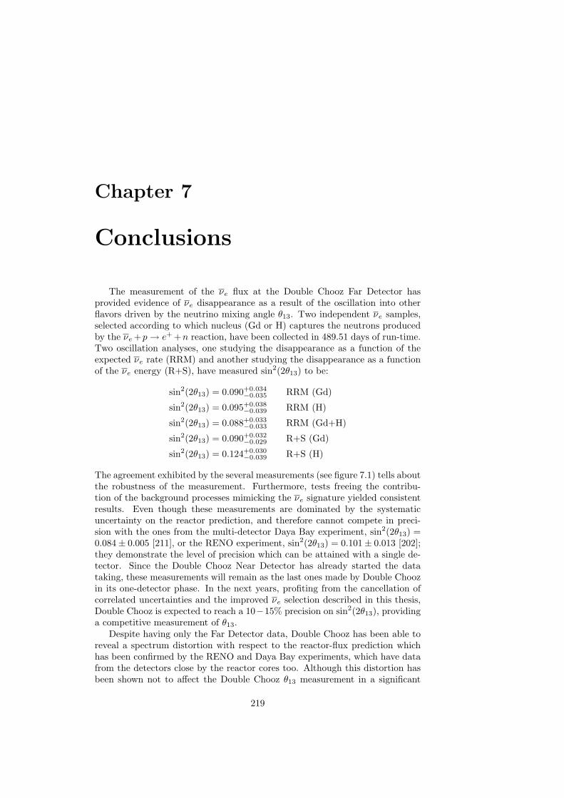
Chapter 7
Conclusions
The measurement of the νe flux at the Double Chooz Far Detector hasprovided evidence of νe disappearance as a result of the oscillation into otherflavors driven by the neutrino mixing angle θ13. Two independent νe samples,selected according to which nucleus (Gd or H) captures the neutrons producedby the νe+p→ e+ +n reaction, have been collected in 489.51 days of run-time.Two oscillation analyses, one studying the disappearance as a function of theexpected νe rate (RRM) and another studying the disappearance as a functionof the νe energy (R+S), have measured sin2(2θ13) to be:
sin2(2θ13) = 0.090+0.034−0.035 RRM (Gd)
sin2(2θ13) = 0.095+0.038−0.039 RRM (H)
sin2(2θ13) = 0.088+0.033−0.033 RRM (Gd+H)
sin2(2θ13) = 0.090+0.032−0.029 R+S (Gd)
sin2(2θ13) = 0.124+0.030−0.039 R+S (H)
The agreement exhibited by the several measurements (see figure 7.1) tells aboutthe robustness of the measurement. Furthermore, tests freeing the contribu-tion of the background processes mimicking the νe signature yielded consistentresults. Even though these measurements are dominated by the systematicuncertainty on the reactor prediction, and therefore cannot compete in preci-sion with the ones from the multi-detector Daya Bay experiment, sin2(2θ13) =0.084± 0.005 [211], or the RENO experiment, sin2(2θ13) = 0.101± 0.013 [202];they demonstrate the level of precision which can be attained with a single de-tector. Since the Double Chooz Near Detector has already started the datataking, these measurements will remain as the last ones made by Double Choozin its one-detector phase. In the next years, profiting from the cancellation ofcorrelated uncertainties and the improved νe selection described in this thesis,Double Chooz is expected to reach a 10−15% precision on sin2(2θ13), providinga competitive measurement of θ13.
Despite having only the Far Detector data, Double Chooz has been able toreveal a spectrum distortion with respect to the reactor-flux prediction whichhas been confirmed by the RENO and Daya Bay experiments, which have datafrom the detectors close by the reactor cores too. Although this distortion hasbeen shown not to affect the Double Chooz θ13 measurement in a significant
219
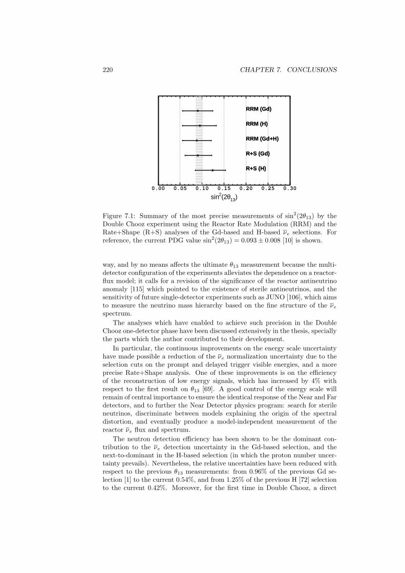
220 CHAPTER 7. CONCLUSIONS
)13θ(22sin0.00 0.05 0.10 0.15 0.20 0.25 0.30
RRM (Gd)
RRM (H)
RRM (Gd+H)
R+S (Gd)
R+S (H)
RRM (Gd)
RRM (H)
RRM (Gd+H)
R+S (Gd)
R+S (H)
Figure 7.1: Summary of the most precise measurements of sin2(2θ13) by theDouble Chooz experiment using the Reactor Rate Modulation (RRM) and theRate+Shape (R+S) analyses of the Gd-based and H-based νe selections. Forreference, the current PDG value sin2(2θ13) = 0.093± 0.008 [10] is shown.
way, and by no means affects the ultimate θ13 measurement because the multi-detector configuration of the experiments alleviates the dependence on a reactor-flux model; it calls for a revision of the significance of the reactor antineutrinoanomaly [115] which pointed to the existence of sterile antineutrinos, and thesensitivity of future single-detector experiments such as JUNO [106], which aimsto measure the neutrino mass hierarchy based on the fine structure of the νespectrum.
The analyses which have enabled to achieve such precision in the DoubleChooz one-detector phase have been discussed extensively in the thesis, speciallythe parts which the author contributed to their development.
In particular, the continuous improvements on the energy scale uncertaintyhave made possible a reduction of the νe normalization uncertainty due to theselection cuts on the prompt and delayed trigger visible energies, and a moreprecise Rate+Shape analysis. One of these improvements is on the efficiencyof the reconstruction of low energy signals, which has increased by 4% withrespect to the first result on θ13 [69]. A good control of the energy scale willremain of central importance to ensure the identical response of the Near and Fardetectors, and to further the Near Detector physics program: search for sterileneutrinos, discriminate between models explaining the origin of the spectraldistortion, and eventually produce a model-independent measurement of thereactor νe flux and spectrum.
The neutron detection efficiency has been shown to be the dominant con-tribution to the νe detection uncertainty in the Gd-based selection, and thenext-to-dominant in the H-based selection (in which the proton number uncer-tainty prevails). Nevertheless, the relative uncertainties have been reduced withrespect to the previous θ13 measurements: from 0.96% of the previous Gd se-lection [1] to the current 0.54%, and from 1.25% of the previous H [72] selectionto the current 0.42%. Moreover, for the first time in Double Chooz, a direct
221
measurement of the neutron selection efficiency in the full volume of the de-tector has been performed using the neutrons from the inverse β-decay (IBD).In the future two-detector measurement in the Gd channel, as a consequenceof the identicalness of the detectors, the contribution of the neutron detectionefficiency uncertainty is expected to reach 0.2%, from the uncorrelated compo-nent between detectors. It will be dominated by the neutron selection efficiency,which is measured most precisely using the IBD neutron source as it has beendescribed in this thesis. The uncertainty on the IBD neutron measurement con-sists of approximately equal statistic and systematic parts. While the statisticsin the Far Detector will continue improving slowly; the systematic uncertaintyarising from the stopping-muon contamination could be brought down if newveto techniques against the stopping-muon background are implemented. An-other advantage of the IBD source to estimate the neutron detection efficiencycompared to the 252Cf is that it does not require to take dedicated calibrationruns, so the detectors can operate with a higher duty cycle.
Given the good performance demonstrated by the Artificial Neural Network-based H selection, which has reached a precision comparable to that of the Gdselection, an extension to include both H and Gd captures at selection level canbe envisioned. This would not only boost the statistics, but also would removethe dominant systematic uncertainty on the neutron detection with a singledetector, the Gd/H fraction, since the two neutron capture possibilities wouldbe treated in an inclusive way. Furthermore, as the Target–Gamma Catcherdistinction would disappear effectively, this would also reduce the uncertaintydue to the migration of neutrons. Consequently, the single-detector physicscapabilities would be enhanced.
The level of precision on θ13 that will be achieved by the three reactor ex-periments (Double Chooz, Daya Bay and RENO) will not be surpassed by otherexperiments in the near future; and unlike the accelerator-based experiments,their measurement does not require assumptions on the values of the other mix-ing angles or the CP violation phase. An eventual combination of the threereactor measurements should provide the most precise θ13 measurement ever,to be used as an input parameter by all the subsequent experiments searchingfor the neutrino mass hierarchy or the CP violation.

222 CHAPTER 7. CONCLUSIONS
References
[1] Double Chooz Collaboration, Y. Abe et al., Reactor electronantineutrino disappearance in the Double Chooz experiment, Phys.Rev.D86 (2012) 052008, [arXiv:1207.6632].
[2] Double Chooz Collaboration, Y. Abe et al., Improved measurements ofthe neutrino mixing angle θ13 with the Double Chooz detector, JHEP1410 (2014) 86 [Erratum ibid. 1502 (2015) 74], [arXiv:1406.7763].
[3] F. Halzen and A. D. Martin, Quarks and Leptons: An IntroductoryCourse in Modern Particle Physics. 1984.
[4] S. L. Glashow, Partial Symmetries of Weak Interactions, Nucl. Phys. 22(1961) 579–588.
[5] S. Weinberg, A Model of Leptons, Phys. Rev. Lett. 19 (1967) 1264–1266.
[6] A. Salam, Weak and Electromagnetic Interactions, Conf. Proc. C680519(1968) 367–377.
[7] F. Englert and R. Brout, Broken Symmetry and the Mass of GaugeVector Mesons, Phys. Rev. Lett. 13 (1964) 321–323.
[8] P. W. Higgs, Broken Symmetries and the Masses of Gauge Bosons,Phys. Rev. Lett. 13 (1964) 508–509.
[9] G. S. Guralnik, C. R. Hagen, and T. W. B. Kibble, Global ConservationLaws and Massless Particles, Phys. Rev. Lett. 13 (1964) 585–587.
[10] Particle Data Group Collaboration, K. A. Olive et al., Review ofParticle Physics, Chin.Phys. C38 (2014) 090001.
[11] ATLAS Collaboration, G. Aad et al., Observation of a new particle inthe search for the Standard Model Higgs boson with the ATLAS detectorat the LHC, Phys. Lett. B716 (2012) 1–29, [arXiv:1207.7214].
[12] CMS Collaboration, S. Chatrchyan et al., Observation of a new boson ata mass of 125 GeV with the CMS experiment at the LHC, Phys. Lett.B716 (2012) 30–61, [arXiv:1207.7235].
[13] M. Goldhaber, L. Grodzins, and A. W. Sunyar, Helicity of Neutrinos,Phys. Rev. 109 (1958) 1015–1017.
[14] L. M. Brown, The idea of the neutrino, Phys. Today 31N9 (1978) 23–28.
223
224 REFERENCES
[15] J. Chadwick, Possible Existence of a Neutron, Nature 129 (1932) 312.
[16] E. Fermi, Trends to a Theory of beta Radiation. (In Italian), NuovoCim. 11 (1934) 1–19.
[17] C. L. Cowan, F. Reines, F. B. Harrison, H. W. Kruse, and A. D.McGuire, Detection of the free neutrino: A Confirmation, Science 124(1956) 103–104.
[18] G. Feinberg, Decays of the mu Meson in the Intermediate-Meson Theory,Phys. Rev. 110 (1958) 1482–1483.
[19] B. Pontecorvo, Electron and Muon Neutrinos, Sov. Phys. JETP 10(1960) 1236–1240. [Zh. Eksp. Teor. Fiz.37,1751(1959)].
[20] G. Danby, J. M. Gaillard, K. A. Goulianos, L. M. Lederman, N. B.Mistry, M. Schwartz, and J. Steinberger, Observation of High-EnergyNeutrino Reactions and the Existence of Two Kinds of Neutrinos, Phys.Rev. Lett. 9 (1962) 36–44.
[21] DONUT Collaboration, K. Kodama et al., Observation of tau neutrinointeractions, Phys. Lett. B504 (2001) 218–224, [hep-ex/0012035].
[22] M. L. Perl et al., Evidence for Anomalous Lepton Production in e+ - e-Annihilation, Phys. Rev. Lett. 35 (1975) 1489–1492.
[23] SLD Electroweak Group, DELPHI, ALEPH, SLD, SLD HeavyFlavour Group, OPAL, LEP Electroweak Working Group, L3Collaboration, S. Schael et al., Precision electroweak measurements onthe Z resonance, Phys. Rept. 427 (2006) 257–454, [hep-ex/0509008].
[24] N. Cabibbo, Unitary Symmetry and Leptonic Decays, Phys. Rev. Lett.10 (1963) 531–533.
[25] M. Kobayashi and T. Maskawa, CP Violation in the RenormalizableTheory of Weak Interaction, Prog. Theor. Phys. 49 (1973) 652–657.
[26] B. Pontecorvo, Neutrino Experiments and the Problem of Conservationof Leptonic Charge, Sov. Phys. JETP 26 (1968) 984–988. [Zh. Eksp.Teor. Fiz.53,1717(1967)].
[27] V. N. Gribov and B. Pontecorvo, Neutrino astronomy and lepton charge,Phys. Lett. B28 (1969) 493.
[28] Z. Maki, M. Nakagawa, and S. Sakata, Remarks on the unified model ofelementary particles, Prog. Theor. Phys. 28 (1962) 870–880.
[29] C. Giunti and C. W. Kim, Fundamentals of Neutrino Physics andAstrophysics. 2007.
[30] B. Kayser, On the Quantum Mechanics of Neutrino Oscillation, Phys.Rev. D24 (1981) 110.
[31] W. Grimus and P. Stockinger, Real oscillations of virtual neutrinos,Phys. Rev. D54 (1996) 3414–3419, [hep-ph/9603430].
REFERENCES 225
[32] L. Wolfenstein, Neutrino Oscillations in Matter, Phys. Rev. D17 (1978)2369–2374.
[33] S. P. Mikheev and A. Yu. Smirnov, Resonance Amplification ofOscillations in Matter and Spectroscopy of Solar Neutrinos, Sov. J.Nucl. Phys. 42 (1985) 913–917. [Yad. Fiz.42,1441(1985)].
[34] S. P. Mikheev and A. Yu. Smirnov, Resonant amplification of neutrinooscillations in matter and solar neutrino spectroscopy, Nuovo Cim. C9(1986) 17–26.
[35] X. Qian and P. Vogel, Neutrino Mass Hierarchy, Prog. Part. Nucl. Phys.83 (2015) 1–30, [arXiv:1505.0189].
[36] J. N. Bahcall, Solar neutrinos. I: Theoretical, Phys. Rev. Lett. 12 (1964)300–302.
[37] R. Davis, Solar neutrinos. II: Experimental, Phys. Rev. Lett. 12 (1964)303–305.
[38] National Nuclear Data Center, “Information extracted from the NuDat 2database.” http://www.nndc.bnl.gov/nudat2/, 2015.
[39] C. Giunti and M. Laveder, Essential solar neutrinos, hep-ph/0301276.
[40] J. N. Bahcall, A. M. Serenelli, and S. Basu, New solar opacities,abundances, helioseismology, and neutrino fluxes, Astrophys. J. 621(2005) L85–L88, [astro-ph/0412440].
[41] B. T. Cleveland, T. Daily, R. Davis, Jr., J. R. Distel, K. Lande, C. K.Lee, P. S. Wildenhain, and J. Ullman, Measurement of the solar electronneutrino flux with the Homestake chlorine detector, Astrophys. J. 496(1998) 505–526.
[42] J. N. Bahcall and M. H. Pinsonneault, What do we (not) knowtheoretically about solar neutrino fluxes?, Phys. Rev. Lett. 92 (2004)121301, [astro-ph/0402114].
[43] GNO Collaboration, M. Altmann et al., Complete results for five yearsof GNO solar neutrino observations, Phys. Lett. B616 (2005) 174–190,[hep-ex/0504037].
[44] SAGE Collaboration, J. N. Abdurashitov et al., Solar neutrino fluxmeasurements by the Soviet-American Gallium Experiment (SAGE) forhalf the 22 year solar cycle, J. Exp. Theor. Phys. 95 (2002) 181–193,[astro-ph/0204245]. [Zh. Eksp. Teor. Fiz.122,211(2002)].
[45] Kamiokande Collaboration, Y. Fukuda et al., Solar neutrino datacovering solar cycle 22, Phys. Rev. Lett. 77 (1996) 1683–1686.
[46] Super-Kamiokande Collaboration, J. Hosaka et al., Solar neutrinomeasurements in Super-Kamiokande-I, Phys. Rev. D73 (2006) 112001,[hep-ex/0508053].
226 REFERENCES
[47] SNO Collaboration, Q. R. Ahmad et al., Direct evidence for neutrinoflavor transformation from neutral current interactions in the SudburyNeutrino Observatory, Phys. Rev. Lett. 89 (2002) 011301,[nucl-ex/0204008].
[48] SNO Collaboration, B. Aharmim et al., Electron energy spectra, fluxes,and day-night asymmetries of B-8 solar neutrinos from measurementswith NaCl dissolved in the heavy-water detector at the Sudbury NeutrinoObservatory, Phys. Rev. C72 (2005) 055502, [nucl-ex/0502021].
[49] SNO Collaboration, B. Aharmim et al., An Independent Measurementof the Total Active B-8 Solar Neutrino Flux Using an Array of He-3Proportional Counters at the Sudbury Neutrino Observatory, Phys. Rev.Lett. 101 (2008) 111301, [arXiv:0806.0989].
[50] Super-Kamiokande Collaboration, S. Fukuda et al., Determination ofsolar neutrino oscillation parameters using 1496 days ofSuper-Kamiokande I data, Phys. Lett. B539 (2002) 179–187,[hep-ex/0205075].
[51] KamLAND Collaboration, A. Gando et al., Reactor On-OffAntineutrino Measurement with KamLAND, Phys. Rev. D88 (2013),no. 3 033001, [arXiv:1303.4667].
[52] Borexino Collaboration, G. Bellini et al., Final results of BorexinoPhase-I on low energy solar neutrino spectroscopy, Phys. Rev. D89(2014), no. 11 112007, [arXiv:1308.0443].
[53] Kamiokande-II Collaboration, K. S. Hirata et al., Experimental Studyof the Atmospheric Neutrino Flux, Phys. Lett. B205 (1988) 416.
[54] R. Becker-Szendy et al., The Electron-neutrino and muon-neutrinocontent of the atmospheric flux, Phys. Rev. D46 (1992) 3720–3724.
[55] Super-Kamiokande Collaboration, R. Wendell et al., Atmosphericneutrino oscillation analysis with sub-leading effects inSuper-Kamiokande I, II, and III, Phys. Rev. D81 (2010) 092004,[arXiv:1002.3471].
[56] Soudan-2 Collaboration, W. W. M. Allison et al., Neutrino oscillationeffects in Soudan-2 upward-stopping muons, Phys. Rev. D72 (2005)052005, [hep-ex/0507068].
[57] MACRO Collaboration, M. Ambrosio et al., Measurements ofatmospheric muon neutrino oscillations, global analysis of the datacollected with MACRO detector, Eur. Phys. J. C36 (2004) 323–339.
[58] K2K Collaboration, M. H. Ahn et al., Measurement of NeutrinoOscillation by the K2K Experiment, Phys. Rev. D74 (2006) 072003,[hep-ex/0606032].
[59] MINOS Collaboration, P. Adamson et al., Combined analysis of νµdisappearance and νµ → νe appearance in MINOS using accelerator andatmospheric neutrinos, Phys.Rev.Lett. 112 (2014) 191801,[arXiv:1403.0867].
REFERENCES 227
[60] T2K Collaboration, K. Abe et al., Precise Measurement of the NeutrinoMixing Parameter θ23 from Muon Neutrino Disappearance in an Off-AxisBeam, Phys. Rev. Lett. 112 (2014), no. 18 181801, [arXiv:1403.1532].
[61] OPERA Collaboration, N. Agafonova et al., Discovery of τ NeutrinoAppearance in the CNGS Neutrino Beam with the OPERA Experiment,Phys. Rev. Lett. 115 (2015), no. 12 121802, [arXiv:1507.0141].
[62] P. Vogel, L. Wen, and C. Zhang, Neutrino Oscillation Studies withReactors, arXiv:1503.0105.
[63] CHOOZ Collaboration, M. Apollonio et al., Search for neutrinooscillations on a long baseline at the CHOOZ nuclear power station,Eur.Phys.J. C27 (2003) 331–374, [hep-ex/0301017].
[64] CHOOZ Collaboration, M. Apollonio et al., Initial results from theCHOOZ long baseline reactor neutrino oscillation experiment, Phys.Lett. B420 (1998) 397–404, [hep-ex/9711002].
[65] F. Boehm et al., Final results from the Palo Verde neutrino oscillationexperiment, Phys. Rev. D64 (2001) 112001, [hep-ex/0107009].
[66] Double Chooz Collaboration, F. Ardellier et al., Double Chooz: ASearch for the neutrino mixing angle theta(13), hep-ex/0606025.
[67] Daya Bay Collaboration, X. Guo et al., A Precision measurement ofthe neutrino mixing angle θ13 using reactor antineutrinos at Daya-Bay,hep-ex/0701029.
[68] RENO Collaboration, J. K. Ahn et al., RENO: An Experiment forNeutrino Oscillation Parameter θ13 Using Reactor Neutrinos atYonggwang, arXiv:1003.1391.
[69] Double Chooz Collaboration, Y. Abe et al., Indication for thedisappearance of reactor electron antineutrinos in the Double Choozexperiment, Phys.Rev.Lett. 108 (2012) 131801, [arXiv:1112.6353].
[70] Daya Bay Collaboration, F. P. An et al., Observation ofelectron-antineutrino disappearance at Daya Bay, Phys.Rev.Lett. 108(2012) 171803, [arXiv:1203.1669].
[71] RENO Collaboration, J. K. Ahn et al., Observation of Reactor ElectronAntineutrino Disappearance in the RENO Experiment, Phys. Rev. Lett.108 (2012) 191802, [arXiv:1204.0626].
[72] Double Chooz Collaboration, Y. Abe et al., First Measurement of θ13
from Delayed Neutron Capture on Hydrogen in the Double ChoozExperiment, Phys.Lett. B723 (2013) 66–70, [arXiv:1301.2948].
[73] Double Chooz Collaboration, C. Buck, The Double Chooz experiment,PoS EPS-HEP2013 (2013) 514.
[74] Double Chooz Collaboration, Y. Abe et al., Background-independentmeasurement of θ13 in Double Chooz, Phys. Lett. B735 (2014) 51–56,[arXiv:1401.5981].
228 REFERENCES
[75] T2K Collaboration, K. Abe et al., Indication of Electron NeutrinoAppearance from an Accelerator-produced Off-axis Muon Neutrino Beam,Phys. Rev. Lett. 107 (2011) 041801, [arXiv:1106.2822].
[76] MINOS Collaboration, P. Adamson et al., Improved search formuon-neutrino to electron-neutrino oscillations in MINOS, Phys. Rev.Lett. 107 (2011) 181802, [arXiv:1108.0015].
[77] M. Freund, Analytic approximations for three neutrino oscillationparameters and probabilities in matter, Phys. Rev. D64 (2001) 053003,[hep-ph/0103300].
[78] T2K Collaboration, K. Abe et al., Observation of Electron NeutrinoAppearance in a Muon Neutrino Beam, Phys. Rev. Lett. 112 (2014)061802, [arXiv:1311.4750].
[79] Troitsk Collaboration, V. N. Aseev et al., An upper limit on electronantineutrino mass from Troitsk experiment, Phys. Rev. D84 (2011)112003, [arXiv:1108.5034].
[80] C. Kraus et al., Final results from phase II of the Mainz neutrino masssearch in tritium beta decay, Eur. Phys. J. C40 (2005) 447–468,[hep-ex/0412056].
[81] KATRIN Collaboration, G. Drexlin, KATRIN: Direct measurement ofa sub-eV neutrino mass, Nucl. Phys. Proc. Suppl. 145 (2005) 263–267.[,263(2005)].
[82] K. Assamagan et al., Upper limit of the muon-neutrino mass andcharged pion mass from momentum analysis of a surface muon beam,Phys. Rev. D53 (1996) 6065–6077.
[83] ALEPH Collaboration, R. Barate et al., An Upper limit on thetau-neutrino mass from three-prong and five-prong tau decays, Eur.Phys. J. C2 (1998) 395–406.
[84] P. Minkowski, µ→ eγ at a Rate of One Out of 109 Muon Decays?, Phys.Lett. B67 (1977) 421–428.
[85] P. Ramond, The Family Group in Grand Unified Theories, inInternational Symposium on Fundamentals of Quantum Theory andQuantum Field Theory Palm Coast, Florida, February 25-March 2,1979, pp. 265–280, 1979. hep-ph/9809459.
[86] M. Gell-Mann, P. Ramond, and R. Slansky, Complex Spinors and UnifiedTheories, Conf. Proc. C790927 (1979) 315–321, [arXiv:1306.4669].
[87] R. N. Mohapatra and G. Senjanovic, Neutrino Mass and SpontaneousParity Violation, Phys. Rev. Lett. 44 (1980) 912.
[88] T. Yanagida, Horizontal Symmetry and Masses of Neutrinos, Conf.Proc. C7902131 (1979) 95–99.
[89] J. Schechter and J. W. F. Valle, Neutrinoless Double beta Decay inSU(2) x U(1) Theories, Phys. Rev. D25 (1982) 2951.
REFERENCES 229
[90] S. Dell’Oro, S. Marcocci, and F. Vissani, New expectations anduncertainties on neutrinoless double beta decay, Phys. Rev. D90 (2014),no. 3 033005, [arXiv:1404.2616].
[91] H. V. Klapdor-Kleingrothaus and I. V. Krivosheina, The evidence for theobservation of 0nu beta beta decay: The identification of 0nu beta betaevents from the full spectra, Mod. Phys. Lett. A21 (2006) 1547–1566.
[92] GERDA Collaboration, M. Agostini et al., Results on NeutrinolessDouble-β Decay of 76Ge from Phase I of the GERDA Experiment, Phys.Rev. Lett. 111 (2013), no. 12 122503, [arXiv:1307.4720].
[93] EXO-200 Collaboration, M. Auger et al., Search for NeutrinolessDouble-Beta Decay in 136Xe with EXO-200, Phys. Rev. Lett. 109 (2012)032505, [arXiv:1205.5608].
[94] EXO-200 Collaboration, J. B. Albert et al., Search for Majorananeutrinos with the first two years of EXO-200 data, Nature 510 (2014)229–234, [arXiv:1402.6956].
[95] KamLAND-Zen Collaboration, A. Gando et al., Limit on Neutrinolessββ Decay of 136Xe from the First Phase of KamLAND-Zen andComparison with the Positive Claim in 76Ge, Phys. Rev. Lett. 110(2013), no. 6 062502, [arXiv:1211.3863].
[96] Planck Collaboration, P. A. R. Ade et al., Planck 2015 results. XIII.Cosmological parameters, arXiv:1502.0158.
[97] G. Mangano, G. Miele, S. Pastor, and M. Peloso, A Precision calculationof the effective number of cosmological neutrinos, Phys. Lett. B534(2002) 8–16, [astro-ph/0111408].
[98] P. Huber, On the determination of anti-neutrino spectra from nuclearreactors, Phys.Rev. C84 (2011) 024617, [arXiv:1106.0687].
[99] M. C. Gonzalez-Garcia, M. Maltoni, and T. Schwetz, Updated fit to threeneutrino mixing: status of leptonic CP violation, JHEP 11 (2014) 052,[arXiv:1409.5439].
[100] NOvA Collaboration, D. S. Ayres et al., NOvA: Proposal to build a 30kiloton off-axis detector to study νµ → νe oscillations in the NuMIbeamline, hep-ex/0503053.
[101] K. Abe et al., Letter of Intent: The Hyper-Kamiokande Experiment —Detector Design and Physics Potential —, arXiv:1109.3262.
[102] LBNE Collaboration, C. Adams et al., The Long-Baseline NeutrinoExperiment: Exploring Fundamental Symmetries of the Universe, 2013.arXiv:1307.7335.
[103] IceCube PINGU Collaboration, M. G. Aartsen et al., Letter of Intent:The Precision IceCube Next Generation Upgrade (PINGU),arXiv:1401.2046.
230 REFERENCES
[104] KM3NeT Collaboration, U. F. Katz, The ORCA Option for KM3NeT,in Proceedings of the 15th International Workshop on NeutrinoTelescopes (Neutel 2013), 2014. arXiv:1402.1022.
[105] ICAL Collaboration, S. Ahmed et al., Physics Potential of the ICALdetector at the India-based Neutrino Observatory (INO),arXiv:1505.0738.
[106] JUNO Collaboration, F. An et al., Neutrino Physics with JUNO,arXiv:1507.0561.
[107] LSND Collaboration, A. Aguilar-Arevalo et al., Evidence for neutrinooscillations from the observation of anti-neutrino(electron) appearance ina anti-neutrino(muon) beam, Phys. Rev. D64 (2001) 112007,[hep-ex/0104049].
[108] KARMEN Collaboration, B. Armbruster et al., Upper limits forneutrino oscillations νµ → øverlineνe from muon decay at rest, Phys.Rev. D65 (2002) 112001, [hep-ex/0203021].
[109] MiniBooNE Collaboration, A. A. Aguilar-Arevalo et al., ImprovedSearch for νµ → νe Oscillations in the MiniBooNE Experiment, Phys.Rev. Lett. 110 (2013) 161801, [arXiv:1207.4809].
[110] MicroBooNE Collaboration, H. Chen et al., Proposal for a NewExperiment Using the Booster and NuMI Neutrino Beamlines:MicroBooNE, .
[111] LArTPC Collaboration, C. Adams et al., LAr1-ND: Testing NeutrinoAnomalies with Multiple LArTPC Detectors at Fermilab, in CommunitySummer Study 2013: Snowmass on the Mississippi (CSS2013)Minneapolis, MN, USA, July 29-August 6, 2013, 2013.arXiv:1309.7987.
[112] D. Gibin and J. Kisiel, ICARUS report to the CXVIII Meeting of SPSC,June 23-24, 2015, Tech. Rep. CERN-SPSC-2015-024. SPSC-SR-163,CERN, Geneva, Jun, 2015.
[113] C. Giunti and M. Laveder, Statistical Significance of the GalliumAnomaly, Phys. Rev. C83 (2011) 065504, [arXiv:1006.3244].
[114] T. A. Mueller, D. Lhuillier, M. Fallot, A. Letourneau, S. Cormon, et al.,Improved Predictions of Reactor Antineutrino Spectra, Phys.Rev. C83(2011) 054615, [arXiv:1101.2663].
[115] G. Mention, M. Fechner, T. Lasserre, T. A. Mueller, D. Lhuillier,M. Cribier, and A. Letourneau, The Reactor Antineutrino Anomaly,Phys. Rev. D83 (2011) 073006, [arXiv:1101.2755].
[116] Borexino Collaboration, G. Bellini et al., SOX: Short distance neutrinoOscillations with BoreXino, JHEP 08 (2013) 038, [arXiv:1304.7721].
[117] A. Gando et al., CeLAND: search for a 4th light neutrino state with a 3PBq 144Ce-144Pr electron antineutrino generator in KamLAND,arXiv:1312.0896.
REFERENCES 231
[118] M. Fukugita and T. Yanagida, Baryogenesis Without Grand Unification,Phys. Lett. B174 (1986) 45.
[119] A. D. Sakharov, Violation of CP Invariance, c Asymmetry, and BaryonAsymmetry of the Universe, Pisma Zh. Eksp. Teor. Fiz. 5 (1967) 32–35.[Usp. Fiz. Nauk161,61(1991)].
[120] Y. Kozlov, L. Mikaelyan, and V. Sinev, Two detector reactor neutrinooscillation experiment Kr2Det at Krasnoyarsk: Status report,Phys.Atom.Nucl. 66 (2003) 469–471, [hep-ph/0109277].
[121] RENO Collaboration, J. K. Ahn et al., Observation of Reactor ElectronAntineutrino Disappearance in the RENO Experiment, Phys.Rev.Lett.108 (2012) 191802, [arXiv:1204.0626].
[122] A. S. Cucoanes, P. Novella, A. Cabrera, M. Fallot, A. Onillon, et al.,Reactor Neutrino Flux Uncertainty Suppression on Multiple DetectorExperiments, arXiv:1501.0035.
[123] P. Vogel and J. F. Beacom, Angular distribution of neutron inverse betadecay, νe + p→ e+ + n, Phys.Rev. D60 (1999) 053003,[hep-ph/9903554].
[124] A. Pichlmaier, V. Varlamov, K. Schreckenbach, and P. Geltenbort,Neutron lifetime measurement with the UCN trap-in-trap MAMBO II,Phys.Lett. B693 (2010) 221–226.
[125] D. H. Wilkinson, Phase space for neutron beta-decay: An update,Nucl.Instrum.Meth. A404 (1998) 305–310.
[126] S. A. Fayans, Radiative Corrections and Recoil Effects in the Reactionνe + P → N + e+ at Low-energies. (In Russian), Sov.J.Nucl.Phys. 42(1985) 590.
[127] C. Aberle, C. Buck, B. Gramlich, F. X. Hartmann, M. Lindner, et al.,Large scale Gd-beta-diketonate based organic liquid scintillator productionfor antineutrino detection, JINST 7 (2012) P06008, [arXiv:1112.5941].
[128] C. Aberle, C. Buck, F. X. Hartmann, and S. Schonert, Light yield andenergy transfer in a new Gd-loaded liquid scintillator, Chem.Phys.Lett.516 (2011) 257–262.
[129] E. Calvo, M. Cerrada, C. Fernandez-Bedoya, I. Gil-Botella,C. Palomares, et al., Characterization of large area photomutipliersunder low magnetic fields: Design and performances of the magneticshielding for the Double Chooz neutrino experiment, Nucl.Instrum.Meth.A621 (2010) 222–230, [arXiv:0905.3246].
[130] D. Dietrich, D. Greiner, J. Jochum, T. Lachenmaier, M. Rohling, et al.,Monte Carlo aided design of the inner muon veto detectors for theDouble Chooz experiment, JINST 7 (2012) P08012, [arXiv:1207.1623].
[131] F. Beissel, A. Cabrera, A. Cucoanes, J. V. Dawson, D. Kryn, et al., TheTrigger and Timing System of the Double Chooz Experiment, JINST 8(2013) T01003, [arXiv:1209.5607].
232 REFERENCES
[132] O. Meplan et al., MURE: MCNP Utility for Reactor Evolution -Description of the methods, first applications and results, in Proceedingsof the European Nuclear Conference (ENC 2005). Nuclear Power for theXXIst Century: From basic research to high-tech industry, 2005.
[133] MURE, MCNP Utility for Reactor Evolution: couples Monte-Carlotransport with fuel burnup calculations, “NEA-1845/01.”http://www.oecd-nea.org/tools/abstract/detail/nea-1845, 2009.
[134] X-5 Monte Carlo Team, MCNP – A General Monte Carlo N-ParticleTransport Code, Version 5, Tech. Rep. LA-UR-03-1987, Los AlamosNational Laboratory, Los Alamos (New Mexico), Apr, 2003.
[135] G. Marleau et al., DRAGON: A Collision Probability Transport Code forCell and Supercell Calculations, Tech. Rep. Report IGE-157, Institut degenie nucleaire, Ecole Polytechnique de Montreal, Montreal, Quebec,1994.
[136] C. L. Jones, A. Bernstein, J. M. Conrad, Z. Djurcic, M. Fallot, et al.,Reactor Simulation for Antineutrino Experiments using DRAGON andMURE, Phys.Rev. D86 (2012) 012001, [arXiv:1109.5379].
[137] V. Kopeikin, L. Mikaelyan, and V. Sinev, Reactor as a source ofantineutrinos: Thermal fission energy, Phys.Atom.Nucl. 67 (2004)1892–1899, [hep-ph/0410100].
[138] M. Fallot and A. Onillon, Reactor plots, Double Chooz InternalDC-doc-3377 (2011).
[139] F. Von Feilitzsch, A. A. Hahn, and K. Schreckenbach, Experimental betaspectra from Pu-239 and U-235 thermal neutron fission products andtheir correlated anti-neutrinos spectra, Phys.Lett. B118 (1982) 162–166.
[140] K. Schreckenbach, G. Colvin, W. Gelletly, and F. Von Feilitzsch,Determination of the anti-neutrino spectrum from U-235 thermalneutron fission products up to 9.5-MeV, Phys.Lett. B160 (1985) 325–330.
[141] A. A. Hahn et al., Anti-neutrino Spectra From 241Pu and 239Pu ThermalNeutron Fission Products, Phys.Lett. B218 (1989) 365–368.
[142] N. Haag et al., Experimental Determination of the AntineutrinoSpectrum of the Fission Products of 238U, Phys.Rev.Lett. 112 (2014),no. 12 122501, [arXiv:1312.5601].
[143] M. Fallot, S. Cormon, M. Estienne, A. Algora, V. M. Bui, et al., Newantineutrino energy spectra predictions from the summation of beta decaybranches of the fission products, Phys.Rev.Lett. 109 (2012) 202504,[arXiv:1208.3877].
[144] Y. Declais et al., Study of reactor anti-neutrino interaction with protonat Bugey nuclear power plant, Phys.Lett. B338 (1994) 383–389.
[145] A. J. Franke, Searching for Reactor Antineutrino Flavor Oscillationswith the Double Chooz Far Detector. PhD thesis, Columbia University,Dec, 2012.
REFERENCES 233
[146] GEANT4 Collaboration, S. Agostinelli et al., GEANT4: A Simulationtoolkit, Nucl.Instrum.Meth. A506 (2003) 250–303.
[147] J. Allison, K. Amako, J. Apostolakis, H. Araujo, P. A. Dubois, et al.,Geant4 developments and applications, IEEE Trans.Nucl.Sci. 53 (2006)270.
[148] D. Motta and S. Schonert, Optical properties of Bialkali photocathodes,Nucl.Instrum.Meth. A539 (2005) 217–235, [physics/0408075].
[149] C. Aberle, C. Buck, F. X. Hartmann, S. Schonert, and S. Wagner, Lightoutput of Double Chooz scintillators for low energy electrons, JINST 6(2011) P11006.
[150] C. Aberle, Optimization, simulation and analysis of the scintillationsignals in the Double Chooz experiment. PhD thesis,Ruperto-Carola-University of Heidelberg, Dec, 2011.
[151] C. Buck and B. Reinhold, Proton Number Tech Note, Double ChoozInternal DC-doc-4211 (2012).
[152] I. Ostrovskiy, Measuring the neutrino mixing angle θ13 with the DoubleChooz Far Detector. PhD thesis, The University of Alabama, 2012.
[153] R. R. Spencer, R. Gwin, and R. Ingle, A Measurement of the AverageNumber of Prompt Neutrons from Spontaneous Fission ofCalifornium-252, Nucl. Sci. and Eng. 80 (1982) 603–629.
[154] A. S. Cucoanes, A Toy Model for the Gamma Spectrum Generated inn-Captures on Gd, Double Chooz Internal DC-doc-3139 (2011).
[155] Y. Abe, T. Akiri, A. Cabrera, B. Courty, J. V. Dawson, et al., TheWaveform Digitiser of the Double Chooz Experiment: Performance andQuantisation Effects on PhotoMultiplier Tube Signals, JINST 8 (2013)P08015, [arXiv:1307.4917].
[156] Y. Abe, C. Buck, A. Cabrera, M. Ishitsuka, G. Pronost,J. Reichenbacher, B. Reinhold, L. F. F. Stokes, and S. Wagner, DCIIIEnergy Blessing candidates (ESv5), Double Chooz InternalDC-doc-5603 (2014).
[157] A. Chyzh, B. Baramsai, J. A. Becker, F. Becvar, T. A. Bredeweg, et al.,Measurement of the Gd-157 (n, gamma) reaction with the DANCEgamma calorimeter array, Phys.Rev. C84 (2011) 014306.
[158] B. Baramsai, G. E. Mitchell, U. Agvaanluvsan, F. Becvar, T. A.Bredeweg, et al., Neutron resonance parameters in Gd-155 measuredwith the DANCE gamma-ray calorimeter array, Phys.Rev. C85 (2012)024622.
[159] Double Chooz Collaboration, Y. Abe et al., Improved measurement ofθ13 in Double Chooz using neutron captures on hydrogen using novelbackground rejection techniques, .
234 REFERENCES
[160] J. I. Crespo-Anadon, Estudio de la emision de luz en los tubosfotomultiplicadores del experimento double chooz, Master’s thesis,Universidad Complutense de Madrid, Jun, 2011.
[161] E. Calvo et al., Toward a better understanding of the glowing: a possibleexplanation of the light emission process, Double Chooz InternalDC-doc-3234 (2011).
[162] Double Chooz Collaboration, Y. Abe et al., Characterization of theSpontaneous Light Emission of the PMTs used in the Double ChoozExperiment, .
[163] R. Roncin, From the measurement of the θ13 mixing angle to the searchfor geo-neutrinos: studying νe with Double Chooz and Borexino. PhDthesis, Universite Paris Diderot (Paris 7) Sorbonne Paris Cite/Universitadegli Studi dell’Aquila, Sep, 2014.
[164] P. Novella, DCIII nGd Candidates: Blessed Plots, Double Chooz InternalDC-doc-5608 (2014).
[165] E. Conover, Muon-induced backgrounds in the Double Chooz neutrinooscillation experiment. PhD thesis, The University of Chicago, Jun,2014.
[166] KamLAND Collaboration, S. Abe et al., Production of RadioactiveIsotopes through Cosmic Muon Spallation in KamLAND, Phys.Rev. C81(2010) 025807, [arXiv:0907.0066].
[167] Double Chooz Collaboration, Y. Abe et al., Precision MuonReconstruction in Double Chooz, Nucl.Inst.Meth.Phys.Res. A (2014)[arXiv:1405.6227].
[168] J. M. Lopez-Castano, Evaluacion del fondo del detector en la medida deθ13 en el experimento Double Chooz. PhD thesis, UniversidadComplutense de Madrid, In preparation, 2015.
[169] J. M. Lopez-Castano, Acc plots to be blessed, Double Chooz InternalDC-doc-5541 (2014).
[170] Double Chooz Collaboration, Y. Abe et al., Direct Measurement ofBackgrounds using Reactor-Off Data in Double Chooz, Phys.Rev. D87(2013) 011102, [arXiv:1210.3748].
[171] A. Hocker, J. Stelzer, F. Tegenfeldt, H. Voss, K. Voss, et al., TMVA -Toolkit for Multivariate Data Analysis, PoS ACAT (2007) 040,[physics/0703039].
[172] R. Brun and F. Rademakers, ROOT: An object oriented data analysisframework, Nucl.Instrum.Meth. A389 (1997) 81–86.
[173] R. Sharankova and J. I. Crespo-Anadon, H-III: ANN plots for blessing,Double Chooz Internal DC-doc-6106 (2015).
[174] G. Pronost, HIII IVV OVV blessing package, Double Chooz InternalDC-doc-6181 (2015).
REFERENCES 235
[175] A. Hourlier, HIII FVV blessing package, Double Chooz InternalDC-doc-6114 (2015).
[176] D. C. A. Group, H-III analysis tech-note, Double Chooz InternalDC-doc-5918 (2015).
[177] A. Meregaglia, MPS-Blessing, Double Chooz Internal DC-doc-6104(2015).
[178] Y. Abe et al., Ortho-positronium observation in the Double ChoozExperiment, JHEP 10 (2014) 32, [arXiv:1407.6913].
[179] A. Cabrera, M. Ishitsuka, A. Meregaglia, and G. Pronost, H-IIICorrelated Background Blessing Package, Double Chooz InternalDC-doc-6105 (2015).
[180] S. L. F. F., HIII LiHe Plots for blessing, Double Chooz InternalDC-doc-6099 (2015).
[181] G. A. Horton-Smith, Composition and volume of scintillator in MC,Double Chooz Internal DC-doc-3188 (2011).
[182] A. Etenko, Slow neutrons modelling, Double Chooz InternalDC-doc-1264 (2009).
[183] A. Etenko, Slow neutrons modelling, Double Chooz InternalDC-doc-1430 (2010).
[184] J. R. Granada, Slow-neutron scattering by molecular gases: A syntheticscattering function, Phys. Rev. B 31 (Apr, 1985) 4167–4177.
[185] Plot produced online using the Evaluated Nuclear Data File (ENDF),National Nuclear Data Center, Brookhaven National LaboratoryENDF/B-VII.1 and CENDL-3.1 databases (2015).
[186] J. Neyman, Outline of a theory of statistical estimation based on theclassical theory of probability, Philosophical Transactions of the RoyalSociety of London. Series A, Mathematical and Physical Sciences 236(1937), no. 767 pp. 333–380.
[187] C. J. Clopper and E. S. Pearson, The use of confidence or fiducial limitsillustrated in the case of the binomial, Biometrika 26 (1934), no. 4 pp.404–413.
[188] “TEfficiency Class Reference.”https://root.cern.ch/doc/master/classTEfficiency.html, 2015.
[189] J. Haser, Neutron Detection Uncertainties in the θ13 Analysis of theDouble Chooz Experiment. PhD thesis, Ruperto-Carola-University ofHeidelberg, Feb, 2015.
[190] J. Haser, n-Gd Neutron Detection Efficiency Volume FactorizationMethod using 252 Cf, Double Chooz Internal DC-doc-5293 (2013).
236 REFERENCES
[191] A. P. Collin, J. I. Crespo-Anadon, J. Haser, and G. Yang, Measurementof the detection systematic uncertainty in the Double Chooz experiment,in Poster in the 37th International Conference on High Energy Physics(ICHEP 2014), 2014.
[192] K. Terao, B. Reinhold, K. Nakajima, J. Maeda, S. Lucht, K. Crum, andR. Carr, nH Analysis Technote, Double Chooz Internal DC-doc-4156(2013).
[193] TRIPOLI-4 version 8.1, 3D general purpose continuous energy MonteCarlo Transport code, “NEA-1716/07.”http://www.oecd-nea.org/tools/abstract/detail/nea-1716, 2013.
[194] J. Haser, “Private communication.” 2015.
[195] P. Novella, H-III Candidates plots for blessing, Double Chooz InternalDC-doc-6096 (2015).
[196] P. Novella, DCIII nGd RRM: blessed plots, Double Chooz InternalDC-doc-5622 (2014).
[197] P. Novella, RRM H-III Blessed plots, Double Chooz InternalDC-doc-6103 (2015).
[198] M. H. Shaevitz, Separating Components of Error Matrices, BooNETechnical Note 253 (2008).
[199] R. Carr and K. Crum, Gd-III Rate+Shape results - blessed, DoubleChooz Internal DC-doc-5610 (2014).
[200] R. Carr and G. Yang, H-III Rate+Shape fit: Candidates for blessing,Double Chooz Internal DC-doc-6146 (2015).
[201] Daya Bay Collaboration, F. P. An et al., Spectral measurement ofelectron antineutrino oscillation amplitude and frequency at Daya Bay,Phys.Rev.Lett. 112 (2014) 061801, [arXiv:1310.6732].
[202] RENO Collaboration, S.-H. Seo, New Results from RENO and The 5MeV Excess, AIP Conf. Proc. 1666 (2015) 080002, [arXiv:1410.7987].
[203] Daya Bay Collaboration, F. P. An et al., Measurement of the ReactorAntineutrino Flux and Spectrum at Daya Bay, arXiv:1508.0423.
[204] D. A. Dwyer and T. J. Langford, Spectral Structure of ElectronAntineutrinos from Nuclear Reactors, Phys. Rev. Lett. 114 (2015), no. 1012502, [arXiv:1407.1281].
[205] M. Chadwick, M. Herman, P. Oblozinsky, et al., ENDF/B-VII.1 nucleardata for science and technology: Cross sections, covariances, fissionproduct yields and decay data, Nuclear Data Sheets 112 (2011), no. 122887 – 2996. Special Issue on ENDF/B-VII.1 Library.
[206] J. Hardy, L. Carraz, B. Jonson, and P. Hansen, The essential decay ofpandemonium: A demonstration of errors in complex beta-decayschemes, Physics Letters B 71 (1977), no. 2 307 – 310.
REFERENCES 237
[207] A. C. Hayes, J. L. Friar, G. T. Garvey, D. Ibeling, G. Jungman,T. Kawano, and R. W. Mills, The Possible Origin and Implications ofthe Shoulder in Reactor Neutrino Spectra, arXiv:1506.0058.
[208] Kellett, M. A. and Bersillon, O. and Mills, R. W., “The JEFF3.1/-3.1.1Radioactive Decay Data and Fission Yields Sub-Libraries. JEFF Report20, NEA Report No. 6287..” http://www.oecd-nea.org/dbforms/data/eva/evatapes/jeff_31/index-JEFF3.1.1.html, 2009.
[209] M. Toups, Chooz Mega-mini Data, Double Chooz InternalDC-doc-1589 (2010).
[210] L. N. Kalousis, Muon flux measurement in the near lab, Double ChoozInternal DC-doc-5006 (2013).
[211] Daya Bay Collaboration, F. P. An et al., A new measurement ofantineutrino oscillation with the full detector configuration at Daya Bay,arXiv:1505.0345.


![Léxico agrícola de Aguaviva (Teruel) y su zona - ifc.dpz.es · z [θ] = interdental fricativa sorda En los rasgos generales mi sincronía coincide totalmente con el valioso estudio](https://static.fdocument.org/doc/165x107/5ba291a409d3f2a1708c131d/lexico-agricola-de-aguaviva-teruel-y-su-zona-ifcdpzes-z-interdental.jpg)