Univariate Time Series Part I
54
Univariate Time Series Jorge Bravo Universidad de Chile July 2015 Jorge Bravo (Universidad de Chile) Time Series July 2015 1 / 54
-
Upload
fena-pino-magna -
Category
Documents
-
view
233 -
download
0
description
Univariate Time Series Lectures
Transcript of Univariate Time Series Part I
Univariate Time Series
Jorge Bravo
Universidad de Chile
July 2015
Jorge Bravo (Universidad de Chile) Time Series July 2015 1 / 54
Univariate Time Series
Outline
1) Stationary stochastic processes
2) Non-stationary stochastic processes
Jorge Bravo (Universidad de Chile) Time Series July 2015 2 / 54
Univariate Time Series
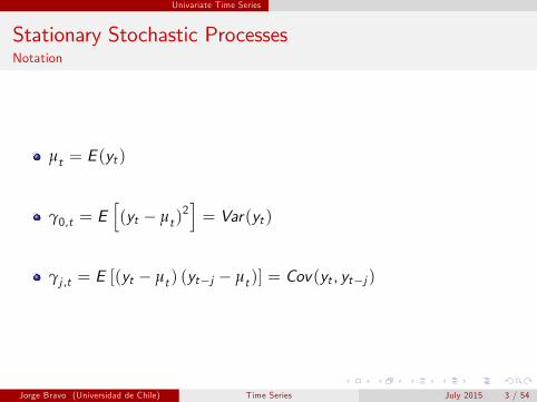
Stationary Stochastic ProcessesNotation
µt = E (yt )
γ0,t = Eh(yt µt )
2i= Var(yt )
γj ,t = E [(yt µt ) (ytj µt )] = Cov(yt , ytj )
Jorge Bravo (Universidad de Chile) Time Series July 2015 3 / 54
Univariate Time Series
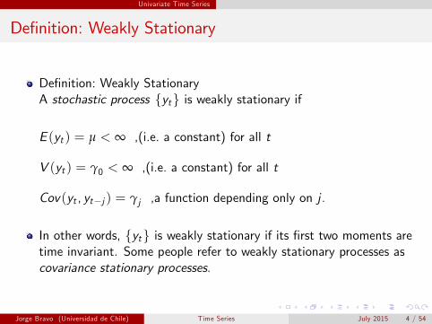
Denition: Weakly Stationary
Denition: Weakly StationaryA stochastic process fytg is weakly stationary if
E (yt ) = µ < ∞ ,(i.e. a constant) for all t
V (yt ) = γ0 < ∞ ,(i.e. a constant) for all t
Cov(yt , ytj ) = γj ,a function depending only on j .
In other words, fytg is weakly stationary if its rst two moments aretime invariant. Some people refer to weakly stationary processes ascovariance stationary processes.
Jorge Bravo (Universidad de Chile) Time Series July 2015 4 / 54
Univariate Time Series
Denition: Strict Stationary
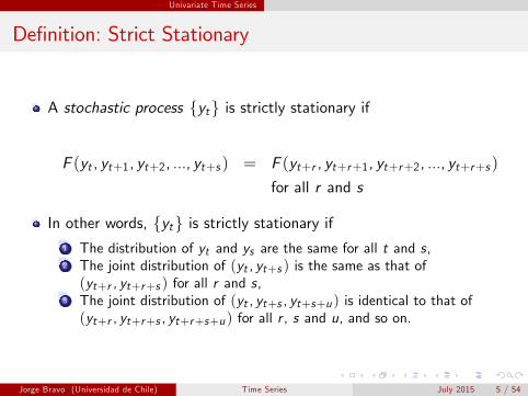
A stochastic process fytg is strictly stationary if
F (yt , yt+1, yt+2, ..., yt+s ) = F (yt+r , yt+r+1, yt+r+2, ..., yt+r+s )
for all r and s
In other words, fytg is strictly stationary if1 The distribution of yt and ys are the same for all t and s,2 The joint distribution of (yt , yt+s ) is the same as that of(yt+r , yt+r+s ) for all r and s,
3 The joint distribution of (yt , yt+s , yt+s+u) is identical to that of(yt+r , yt+r+s , yt+r+s+u) for all r , s and u, and so on.
Jorge Bravo (Universidad de Chile) Time Series July 2015 5 / 54
Univariate Time Series
Denition: Strict Stationary
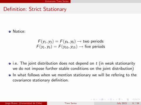
Notice:
F (y1, y3) = F (y4, y6)! two periodsF (y1, y5) = F (y10, y15)! ve periods
i.e. The joint distribution does not depend on t (in weak stationaritywe do not impose further stable conditions on the joint distribution)
In what follows when we mention stationary we will be refering to thecovariance stationary denition.
Jorge Bravo (Universidad de Chile) Time Series July 2015 6 / 54
Univariate Time Series
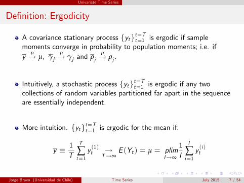
Denition: Ergodicity
A covariance stationary process fytgt=Tt=1 is ergodic if samplemoments converge in probability to population moments; i.e. ify
p! µ, γjp! γj and ρj
p! ρj .
Intuitively, a stochastic process fytgt=Tt=1 is ergodic if any twocollections of random variables partitioned far apart in the sequenceare essentially independent.
More intuition. fytgt=Tt=1 is ergodic for the mean if:
y 1T
T
∑t=1y (1)t !
T!∞E (Yt ) = µ = plim
I!∞
1I
I
∑i=1y (i )t
Jorge Bravo (Universidad de Chile) Time Series July 2015 7 / 54
Univariate Time Series
White Noise Process
It is the building block for our time series models.
εt for t = 1, 2, . . . ,T , is a white noise if:1 E [εt ] = E [εt jεt1,εt2,...] = E [εt jall information en t 1] = 02 Cov(εt , εtj ) = 0, for all t and j .3 Var [εt ] = Var [εt jεt1,εt2,...] = Var [εt jall information en t 1] =
σ2ε
The rst and second properties are the absence of any serialcorrelation or predictability. The third property is conditionalhomoskedasticity or a constant conditional variance.
Jorge Bravo (Universidad de Chile) Time Series July 2015 8 / 54
Univariate Time Series
White Noise Process
Remarks:
Notation: εt sWN(0, σ2ε )This process is a Gaussian white noise process if εt s N(0, σ2ε )By construction it is a stationary process (a collection of uncorrelatedrandom variables with mean 0)Example: the error term of a classical linear regression model is a whitenoise.
Jorge Bravo (Universidad de Chile) Time Series July 2015 9 / 54
Univariate Time Series
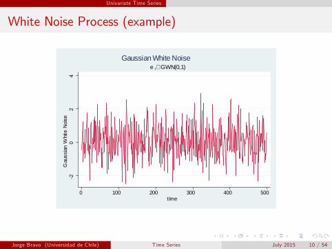
White Noise Process (example)
20
24
Gau
ssia
n W
hite
Noi
se
0 100 200 300 400 500time
e t∼ GWN(0,1)Gaussian White Noise
Jorge Bravo (Universidad de Chile) Time Series July 2015 10 / 54
Univariate Time Series
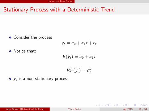
Stationary Process with a Deterministic Trend
Consider the processyt = α0 + α1t + εt
Notice that:E (yt ) = α0 + α1t
Var(yt ) = σ2ε
yt is a non-stationary process.
Jorge Bravo (Universidad de Chile) Time Series July 2015 11 / 54
Univariate Time Series
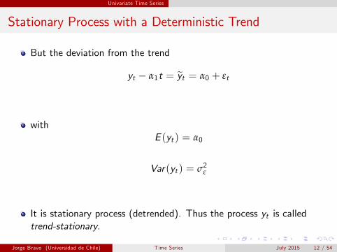
Stationary Process with a Deterministic Trend
But the deviation from the trend
yt α1t = eyt = α0 + εt
withE (yt ) = α0
Var(yt ) = σ2ε
It is stationary process (detrended). Thus the process yt is calledtrend-stationary.
Jorge Bravo (Universidad de Chile) Time Series July 2015 12 / 54
Univariate Time Series
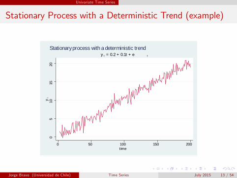
Stationary Process with a Deterministic Trend (example)
05
1015
20y
t
0 50 100 150 200time
y t = 0.2 + 0.1t + e t
Stationary process with a deterministic trend
Jorge Bravo (Universidad de Chile) Time Series July 2015 13 / 54
Univariate Time Series
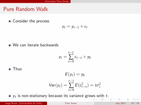
Pure Random Walk
Consider the processyt = yt1 + εt
We can iterate backwards
yt =t1∑s=0
εts + y0
ThusE (yt ) = y0
Var(yt ) =t1∑s=0
E (ε2ts ) = tσ2ε
yt is non-stationary because its variance grows with t.
Jorge Bravo (Universidad de Chile) Time Series July 2015 14 / 54
Univariate Time Series
Random Walk with Drift
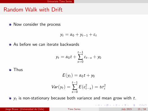
Now consider the process
yt = α0 + yt1 + εt
As before we can iterate backwards
yt = α0t +t1∑s=0
εts + y0
ThusE (yt ) = α0t + y0
Var(yt ) =t1∑s=0
E (ε2ts ) = tσ2ε
yt is non-stationary because both variance and mean grow with t.
Jorge Bravo (Universidad de Chile) Time Series July 2015 15 / 54
Univariate Time Series
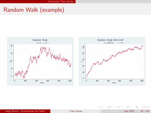
Random Walk (example)0
1020
3040
yt
0 200 400 600 800 1000time
y t = y t 1 + e t
Random W alk
020
4060
8010
0y
t0 200 400 600 800 1000
time
y t = 0.15 + y t 1 + e t
Random W alk W ith Drif t
Jorge Bravo (Universidad de Chile) Time Series July 2015 16 / 54
Univariate Time Series
Random Walk with Drift
Remarks
The e¤ect of the initial value, y0, stays in the process.The innovations, εts , are accumulated to a random walk, ∑t1s=0 εts .This is denoted a stochastic trend.Note that shocks have permanent e¤ects.In the case of deterministic trend shocks have transitory e¤ects. Why?
Jorge Bravo (Universidad de Chile) Time Series July 2015 17 / 54
Univariate Time Series
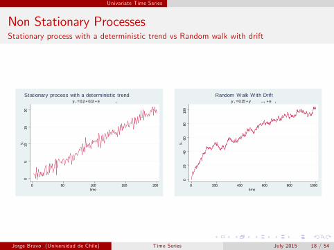
Non Stationary ProcessesStationary process with a deterministic trend vs Random walk with drift
05
1015
20y
t
0 50 100 150 200time
y t = 0.2 + 0.1t + e t
Stat ionary process with a deterministic trend
020
4060
8010
0y
t
0 200 400 600 800 1000time
y t = 0.15 + y t 1 + e t
Random W alk W ith Drif t
Jorge Bravo (Universidad de Chile) Time Series July 2015 18 / 54
Univariate Time Series
Univariate Stationary Time Series Models
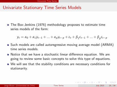
The Box-Jenkins (1976) methodology proposes to estimate timeseries models of the form:
yt = α0 + α1yt1 + ...+ αpytp + εt + β1εt1 + ...+ βpεtp
Such models are called autoregressive moving average model (ARMA)time series models.
Notice that we have a stochastic linear di¤erence equation. We aregoing to review some basic concepts to solve this type of equations.
We will see that the stability conditions are necessary conditions forstationarity.
Jorge Bravo (Universidad de Chile) Time Series July 2015 19 / 54
Univariate Time Series
Univariate Stationary Time Series Models
In what follows we will develop the tools used to identify and estimateARMA models following the Box-Jenkins methodology.
These models are useful for:
Statistical hypothesis testing (to prove some theory)Forecasting
Some examples?
Jorge Bravo (Universidad de Chile) Time Series July 2015 20 / 54
Univariate Time Series
Univariate Stationary Time Series Models
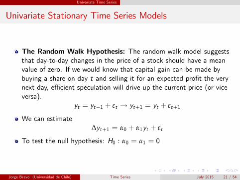
The Random Walk Hypothesis: The random walk model suggeststhat day-to-day changes in the price of a stock should have a meanvalue of zero. If we would know that capital gain can be made bybuying a share on day t and selling it for an expected prot the verynext day, e¢ cient speculation will drive up the current price (or viceversa).
yt = yt1 + εt ! yt+1 = yt + εt+1
We can estimate∆yt+1 = α0 + α1yt + εt
To test the null hypothesis: H0 : α0 = α1 = 0
Jorge Bravo (Universidad de Chile) Time Series July 2015 21 / 54
Univariate Time Series
Univariate Stationary Time Series Models
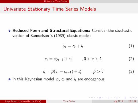
Reduced Form and Structural Equations: Consider the stochasticversion of Samuelson´s (1939) classic model:
yt = ct + it (1)
ct = αyt1 + εct , 0 < α < 1 (2)
it = β(ct ct1) + εit , β > 0 (3)
In this Keynesian model yt , ct and it are endogenous.
Jorge Bravo (Universidad de Chile) Time Series July 2015 22 / 54
Univariate Time Series
Univariate Stationary Time Series Models
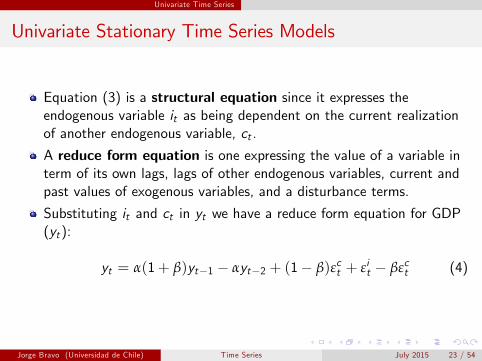
Equation (3) is a structural equation since it expresses theendogenous variable it as being dependent on the current realizationof another endogenous variable, ct .
A reduce form equation is one expressing the value of a variable interm of its own lags, lags of other endogenous variables, current andpast values of exogenous variables, and a disturbance terms.
Substituting it and ct in yt we have a reduce form equation for GDP(yt):
yt = α(1+ β)yt1 αyt2 + (1 β)εct + εit βεct (4)
Jorge Bravo (Universidad de Chile) Time Series July 2015 23 / 54
Univariate Time Series
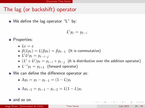
The lag (or backshift) operator
We dene the lag operator Lby:
Liyt = yti
Properties:
Lc = cβ(Lyt ) = L(βyt ) = βyt1 (It is commutative)LiLjyt = ytij(Li + Lj )yt = yti + ytj /(it is distributive over the addition operator)Li yt = yt+1 (forward operator)
We can dene the di¤erence operator as:
∆yt = yt yt1 = (1 L)yt
∆yt1 = yt1 yt2 = L(1 L)yt
and so on.Jorge Bravo (Universidad de Chile) Time Series July 2015 24 / 54
Univariate Time Series
Moving Average Process
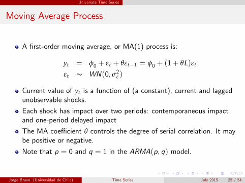
A rst-order moving average, or MA(1) process is:
yt = φ0 + εt + θεt1 = φ0 + (1+ θL)εtεt s WN(0, σ2ε )
Current value of yt is a function of (a constant), current and laggedunobservable shocks.
Each shock has impact over two periods: contemporaneous impactand one-period delayed impact
The MA coe¢ cient θ controls the degree of serial correlation. It maybe positive or negative.
Note that p = 0 and q = 1 in the ARMA(p, q) model.
Jorge Bravo (Universidad de Chile) Time Series July 2015 25 / 54
Univariate Time Series
MA(1) Process
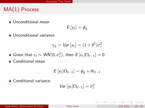
Unconditional meanE [yt ] = φ0
Unconditional variance
γ0 = Var [yt ] = (1+ θ2)σ2ε
Given that εt sWN(0, σ2ε ), then E [εt jΩt1] = 0
Conditional mean
E [yt jΩt1] = φ0 + θεt1
Conditional varianceVar [yt jΩt1] = σ2ε
Jorge Bravo (Universidad de Chile) Time Series July 2015 26 / 54
Univariate Time Series
MA(1) Process
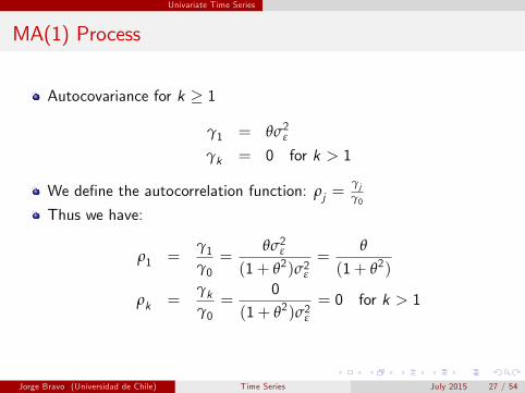
Autocovariance for k 1
γ1 = θσ2ε
γk = 0 for k > 1
We dene the autocorrelation function: ρj =γjγ0
Thus we have:
ρ1 =γ1γ0=
θσ2ε(1+ θ2)σ2ε
=θ
(1+ θ2)
ρk =γkγ0=
0
(1+ θ2)σ2ε= 0 for k > 1
Jorge Bravo (Universidad de Chile) Time Series July 2015 27 / 54
Univariate Time Series
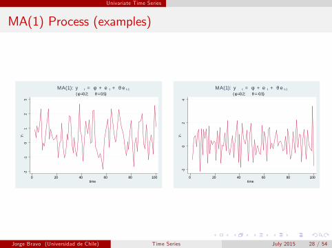
MA(1) Process (examples)2
10
12
3y
t
0 20 40 60 80 100time
( φ =0.2; θ = 0.5)MA(1): y t = φ + e t + θ e t1
20
24
yt
0 20 40 60 80 100time
( φ =0.2; θ = 0.5)MA(1): y t = φ + e t + θ e t1
Jorge Bravo (Universidad de Chile) Time Series July 2015 28 / 54
Univariate Time Series
MA(2) Process
A second-order moving average, or MA(2) process is:
yt = φ0 + εt + θ1εt1 + θ2εt2 = φ0 + (1+ θ1L+ θ2L2)εtεt s WN(0, σ2ε )
Now we have p = 0 and q = 2 in the ARMA(p, q) model.
Jorge Bravo (Universidad de Chile) Time Series July 2015 29 / 54
Univariate Time Series
MA(2) Process
Properties
Unconditional meanE [yt ] = φ0
Unconditional variance
γ0 = Var [yt ] = (1+ θ21 + θ22)σ2ε
Given that εt sWN(0, σ2ε ), then E [εt jΩt1] = 0
Conditional mean
E [yt jΩt1] = φ0 + θ1εt1 + θ2εt2
Conditional varianceVar [yt jΩt1] = σ2ε
Jorge Bravo (Universidad de Chile) Time Series July 2015 30 / 54
Univariate Time Series
MA(2) Process
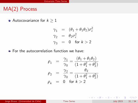
Autocovariance for k 1
γ1 = (θ1 + θ1θ2)σ2ε
γ2 = θ2σ2ε
γ3 = 0 for k > 2
For the autocorrelation function we have:
ρ1 =γ1γ0=
(θ1 + θ1θ2)
(1+ θ21 + θ22)
ρ2 =γ2γ0=
θ2
(1+ θ21 + θ22)
ρk = 0 for k > 2
Jorge Bravo (Universidad de Chile) Time Series July 2015 31 / 54
Univariate Time Series
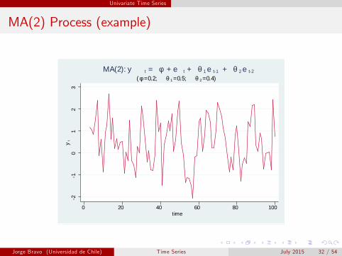
MA(2) Process (example)
21
01
23
yt
0 20 40 60 80 100time
( φ =0.2; θ 1 =0.5; θ 2 =0.4)MA(2): y t = φ + e t + θ 1 e t1 + θ 2 e t2
Jorge Bravo (Universidad de Chile) Time Series July 2015 32 / 54
Univariate Time Series
MA(q) Process
A q-order moving average, or MA(q) process is:
yt = φ0 + εt + θ1εt1 + θ2εt2 + ...+ θqεtq
= φ0 + (1+ θ1L+ θ2L2 + ...+ θqLq)εtεt s WN(0, σ2ε )
Now we have ARMA(0, q) model.
Jorge Bravo (Universidad de Chile) Time Series July 2015 33 / 54
Univariate Time Series
MA(q) Process
Unconditional meanE [yt ] = φ0
Unconditional variance
γ0 = (1+ θ21 + θ22 + ...+ θ2q)σ2ε
Given that εt sWN(0, σ2ε ), then E [εt jΩt1] = 0
Conditional mean
E [yt jΩt1] = φ0 + θ1εt1 + θ2εt2 + ...+ θqεtq
Conditional varianceVar [yt jΩt1] = σ2ε
Jorge Bravo (Universidad de Chile) Time Series July 2015 34 / 54
Univariate Time Series
MA(q) Process
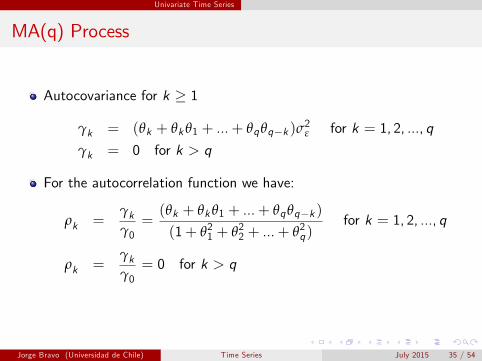
Autocovariance for k 1
γk = (θk + θk θ1 + ...+ θqθqk )σ2ε for k = 1, 2, ..., q
γk = 0 for k > q
For the autocorrelation function we have:
ρk =γkγ0=(θk + θk θ1 + ...+ θqθqk )
(1+ θ21 + θ22 + ...+ θ2q)for k = 1, 2, ..., q
ρk =γkγ0= 0 for k > q
Jorge Bravo (Universidad de Chile) Time Series July 2015 35 / 54
Univariate Time Series
Autoregressive Process
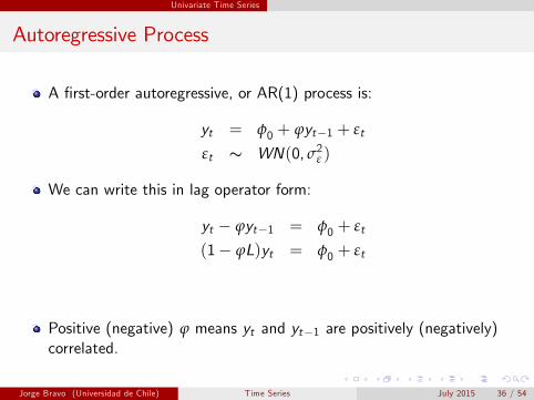
A rst-order autoregressive, or AR(1) process is:
yt = φ0 + ϕyt1 + εt
εt s WN(0, σ2ε )
We can write this in lag operator form:
yt ϕyt1 = φ0 + εt
(1 ϕL)yt = φ0 + εt
Positive (negative) ϕ means yt and yt1 are positively (negatively)correlated.
Jorge Bravo (Universidad de Chile) Time Series July 2015 36 / 54
Univariate Time Series
AR(1) Process
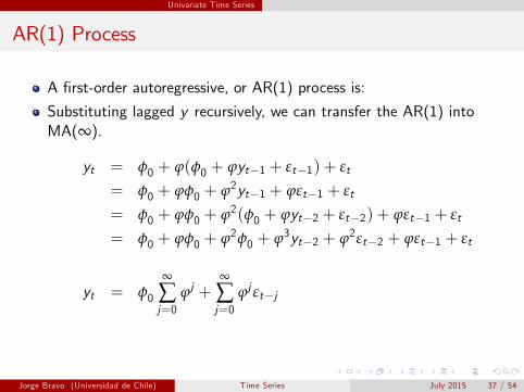
A rst-order autoregressive, or AR(1) process is:
Substituting lagged y recursively, we can transfer the AR(1) intoMA(∞).
yt = φ0 + ϕ(φ0 + ϕyt1 + εt1) + εt
= φ0 + ϕφ0 + ϕ2yt1 + ϕεt1 + εt
= φ0 + ϕφ0 + ϕ2(φ0 + ϕyt2 + εt2) + ϕεt1 + εt
= φ0 + ϕφ0 + ϕ2φ0 + ϕ3yt2 + ϕ2εt2 + ϕεt1 + εt
yt = φ0
∞
∑j=0
ϕj +∞
∑j=0
ϕj εtj
Jorge Bravo (Universidad de Chile) Time Series July 2015 37 / 54
Univariate Time Series
AR(1) Process
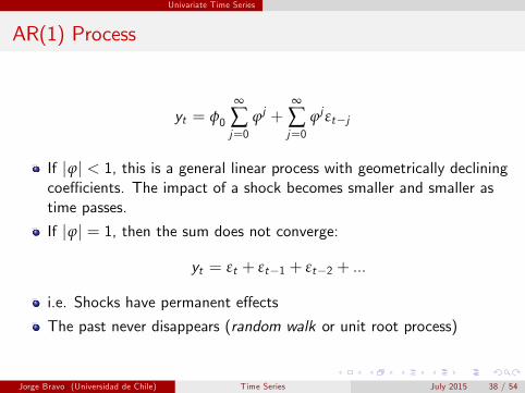
yt = φ0
∞
∑j=0
ϕj +∞
∑j=0
ϕj εtj
If jϕj < 1, this is a general linear process with geometrically decliningcoe¢ cients. The impact of a shock becomes smaller and smaller astime passes.
If jϕj = 1, then the sum does not converge:
yt = εt + εt1 + εt2 + ...
i.e. Shocks have permanent e¤ects
The past never disappears (random walk or unit root process)
Jorge Bravo (Universidad de Chile) Time Series July 2015 38 / 54
Univariate Time Series
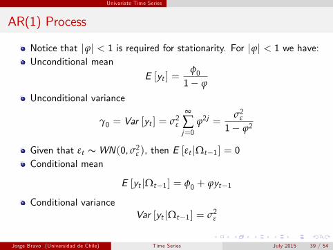
AR(1) Process
Notice that jϕj < 1 is required for stationarity. For jϕj < 1 we have:Unconditional mean
E [yt ] =φ01 ϕ
Unconditional variance
γ0 = Var [yt ] = σ2ε
∞
∑j=0
ϕ2j =σ2ε
1 ϕ2
Given that εt sWN(0, σ2ε ), then E [εt jΩt1] = 0Conditional mean
E [yt jΩt1] = φ0 + ϕyt1
Conditional varianceVar [yt jΩt1] = σ2ε
Jorge Bravo (Universidad de Chile) Time Series July 2015 39 / 54
Univariate Time Series
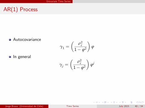
AR(1) Process
Autocovariance
γ1 =
σ2ε
1 ϕ2
ϕ
In general
γj =
σ2ε
1 ϕ2
ϕj
Jorge Bravo (Universidad de Chile) Time Series July 2015 40 / 54
Univariate Time Series
AR(1) Process
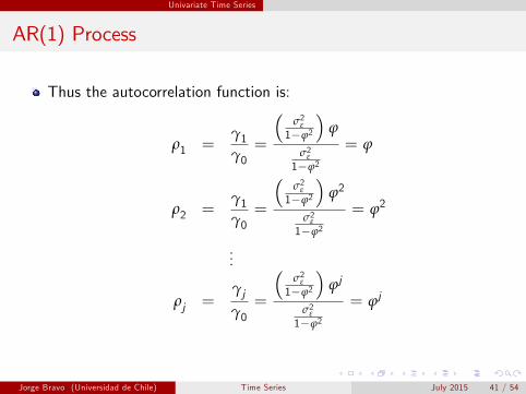
Thus the autocorrelation function is:
ρ1 =γ1γ0=
σ2ε1ϕ2
ϕ
σ2ε1ϕ2
= ϕ
ρ2 =γ1γ0=
σ2ε1ϕ2
ϕ2
σ2ε1ϕ2
= ϕ2
...
ρj =γjγ0=
σ2ε1ϕ2
ϕj
σ2ε1ϕ2
= ϕj
Jorge Bravo (Universidad de Chile) Time Series July 2015 41 / 54
Univariate Time Series
AR(1) Process
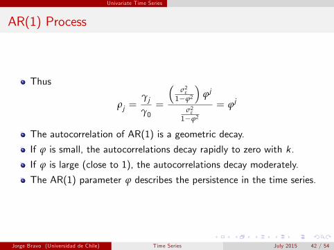
Thus
ρj =γjγ0=
σ2ε1ϕ2
ϕj
σ2ε1ϕ2
= ϕj
The autocorrelation of AR(1) is a geometric decay.
If ϕ is small, the autocorrelations decay rapidly to zero with k.
If ϕ is large (close to 1), the autocorrelations decay moderately.
The AR(1) parameter ϕ describes the persistence in the time series.
Jorge Bravo (Universidad de Chile) Time Series July 2015 42 / 54
Univariate Time Series
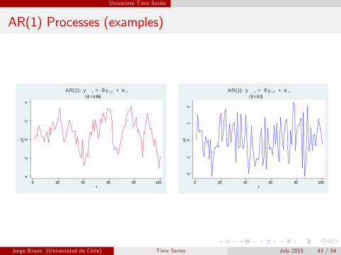
AR(1) Processes (examples)4
20
24
y1
0 20 40 60 80 100t
( θ = 0.95)AR(1): y t = θ y t1 + e t
21
01
2y2
0 20 40 60 80 100t
( θ = 0.2)AR(1): y t = θ y t1 + e t
Jorge Bravo (Universidad de Chile) Time Series July 2015 43 / 54
Univariate Time Series
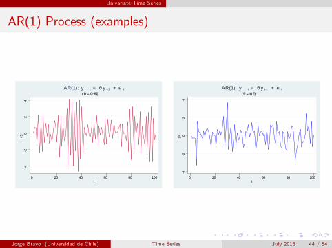
AR(1) Process (examples)4
20
24
y3
0 20 40 60 80 100t
( θ = 0.95)AR(1): y t = θ y t1 + e t
42
02
4y4
0 20 40 60 80 100t
( θ = 0.2)AR(1): y t = θ y t1 + e t
Jorge Bravo (Universidad de Chile) Time Series July 2015 44 / 54
Univariate Time Series
AR(2) Process
A second-order autoregressive, or AR(2) process is:
yt = φ0 + ϕ1yt1 + ϕ2yt2 + εt
εt s WN(0, σ2ε )
We can write this in lag operator form:
yt ϕ1yt1 ϕ2yt2 = φ0 + εt
(1 ϕ1L ϕ2L2)yt = φ0 + εt
Φ(L)yt = φ0 + εt
Characteristic equation:
1 ϕ1x ϕ2x2 = 0
yt is covariance stationary if all roots of the characteristic equationare outside the unit circle. (stationarity condition).
Jorge Bravo (Universidad de Chile) Time Series July 2015 45 / 54
Univariate Time Series
AR(2) Process
In the case of AR(1) we have:
1 ϕ1L = 0) L =
1ϕ1 > 1, jϕ1j < 1
In the case of AR(2) we have:
1 ϕ1L ϕ2L = 0) L =
ϕ1
qϕ21 4ϕ2
2ϕ2
> 1Example:
yt = 0.7yt1 + 0.35yt2(1 0.7L 0.35L2)yt = 0
Characteristic equation:
1 0.7x 0.35x2 = 0
Jorge Bravo (Universidad de Chile) Time Series July 2015 46 / 54
Univariate Time Series
AR(2) Process
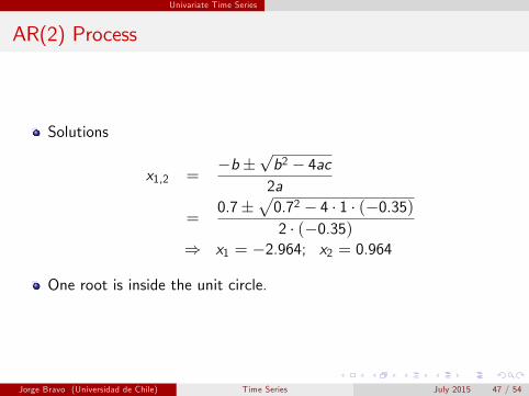
Solutions
x1,2 =b
pb2 4ac2a
=0.7
p0.72 4 1 (0.35)2 (0.35)
) x1 = 2.964; x2 = 0.964
One root is inside the unit circle.
Jorge Bravo (Universidad de Chile) Time Series July 2015 47 / 54
Univariate Time Series
AR(2) Process
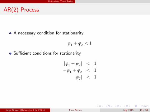
A necessary condition for stationarity
ϕ1 + ϕ2 < 1
Su¢ cient conditions for stationarity
jϕ1 + ϕ2j < 1
ϕ1 + ϕ2 < 1
jϕ2j < 1
Jorge Bravo (Universidad de Chile) Time Series July 2015 48 / 54
Univariate Time Series
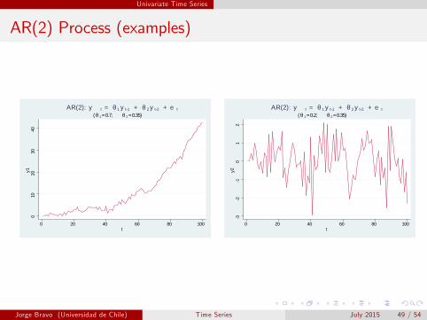
AR(2) Process (examples)0
1020
3040
y1
0 20 40 60 80 100t
( θ 1 = 0.7; θ 2 = 0.35)AR(2): y t = θ 1 y t1 + θ 2 y t2 + e t
32
10
12
y20 20 40 60 80 100
t
( θ 1 = 0.2; θ 2 = 0.35)AR(2): y t = θ 1 y t1 + θ 2 y t2 + e t
Jorge Bravo (Universidad de Chile) Time Series July 2015 49 / 54
Univariate Time Series
AR(2) Process
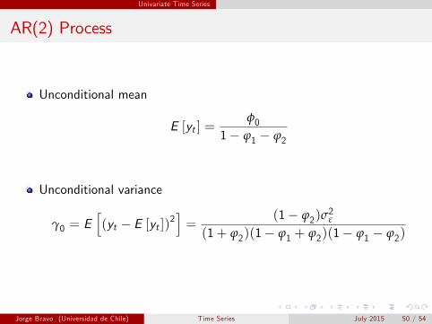
Unconditional mean
E [yt ] =φ0
1 ϕ1 ϕ2
Unconditional variance
γ0 = Eh(yt E [yt ])2
i=
(1 ϕ2)σ2ε
(1+ ϕ2)(1 ϕ1 + ϕ2)(1 ϕ1 ϕ2)
Jorge Bravo (Universidad de Chile) Time Series July 2015 50 / 54
Univariate Time Series
AR(2) Process
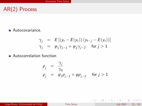
Autocovariance.
γj = E [(yt E (yt )) (ytj E (yt ))]γj = ϕ1γj1 + ϕ2γj2 for j > 1
Autocorrelation function
ρj =γjγ0
ρj = ϕ1ρj1 + ϕρj2 for j > 1
Jorge Bravo (Universidad de Chile) Time Series July 2015 51 / 54
Univariate Time Series
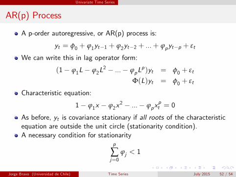
AR(p) Process
A p-order autoregressive, or AR(p) process is:
yt = φ0 + ϕ1yt1 + ϕ2yt2 + ...+ ϕpytp + εt
We can write this in lag operator form:
(1 ϕ1L ϕ2L2 ... ϕpL
p)yt = φ0 + εt
Φ(L)yt = φ0 + εt
Characteristic equation:
1 ϕ1x ϕ2x2 ... ϕpx
pt = 0
As before, yt is covariance stationary if all roots of the characteristicequation are outside the unit circle (stationarity condition).A necessary condition for stationarity
p
∑j=0
ϕj < 1
Jorge Bravo (Universidad de Chile) Time Series July 2015 52 / 54
Univariate Time Series
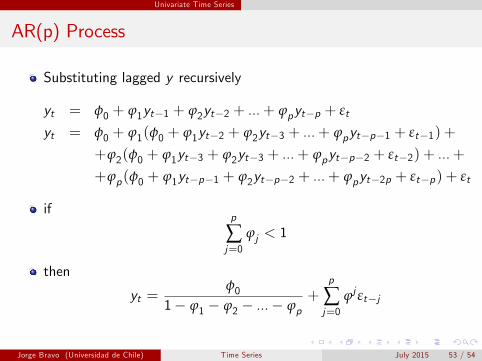
AR(p) Process
Substituting lagged y recursively
yt = φ0 + ϕ1yt1 + ϕ2yt2 + ...+ ϕpytp + εt
yt = φ0 + ϕ1(φ0 + ϕ1yt2 + ϕ2yt3 + ...+ ϕpytp1 + εt1) +
+ϕ2(φ0 + ϕ1yt3 + ϕ2yt3 + ...+ ϕpytp2 + εt2) + ...+
+ϕp(φ0 + ϕ1ytp1 + ϕ2ytp2 + ...+ ϕpyt2p + εtp) + εt
ifp
∑j=0
ϕj < 1
then
yt =φ0
1 ϕ1 ϕ2 ... ϕp+
p
∑j=0
ϕj εtj
Jorge Bravo (Universidad de Chile) Time Series July 2015 53 / 54
Univariate Time Series
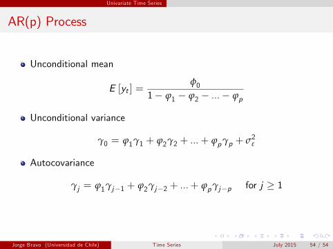
AR(p) Process
Unconditional mean
E [yt ] =φ0
1 ϕ1 ϕ2 ... ϕp
Unconditional variance
γ0 = ϕ1γ1 + ϕ2γ2 + ...+ ϕpγp + σ2ε
Autocovariance
γj = ϕ1γj1 + ϕ2γj2 + ...+ ϕpγjp for j 1
Jorge Bravo (Universidad de Chile) Time Series July 2015 54 / 54