Unadulterated spectral function of low-energy quasiparticles

Unadulterated spectral function of low-energy quasiparticles

Evtushinsky Daniil

Institute of Metal Physics,Kiev, Ukraine

Moscow Institute of Physics and Technology

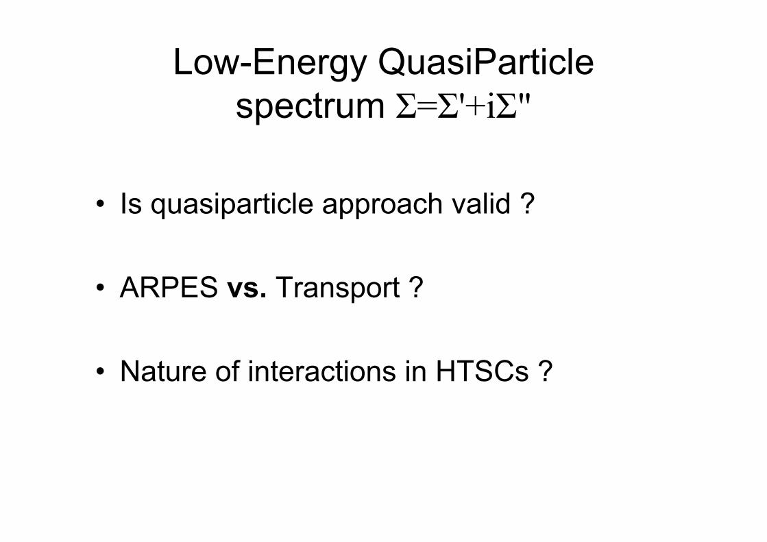
Low-Energy QuasiParticlespectrum Σ=Σ'+iΣ"

• Is quasiparticle approach valid ?

• ARPES vs. Transport ?

• Nature of interactions in HTSCs ?

• Offset at ω → 0 and at T → 0 ?

• Behavior near TC ?

• Evolution with doping?

Questions to behavior of Σ"∼1/τ

Problems

• How to remove resolution effectsaccurately?

R-?

• How to disentangle impurity scatteringfrom quasiparticle interaction?

Σ"int=Σ"-Σ"imp

Total response function

• RA – Analyzer• Remains constant• Easy to measure

• RS – Sample Surface• Varies with space and time• Difficult to measure

R=RA ⊗ RS

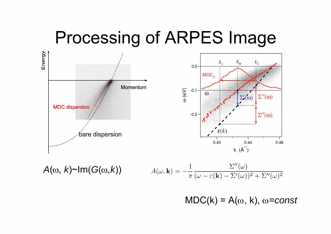
Processing of ARPES Image

MDC(k) = A(ω, k), ω=const

bare dispersion

A(ω, k)~Im(G(ω,k))

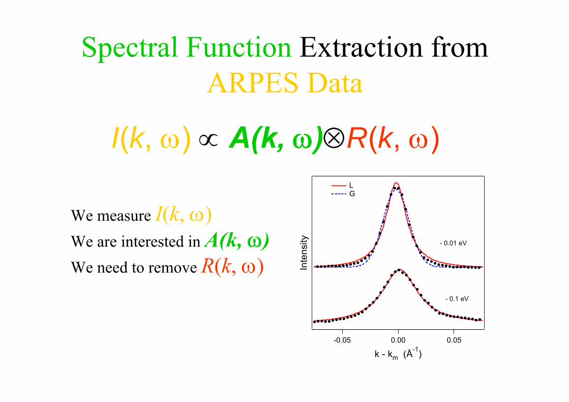
Spectral Function Extraction from ARPES Data

I(k, ω) ∝ A(k, ω)⊗R(k, ω)

Inte

nsity

-0.05 0.00 0.05

k - km (Å-1)

L G

- 0.01 eV

- 0.1 eV

We measure I(k, ω)We are interested in A(k, ω)We need to remove R(k, ω)

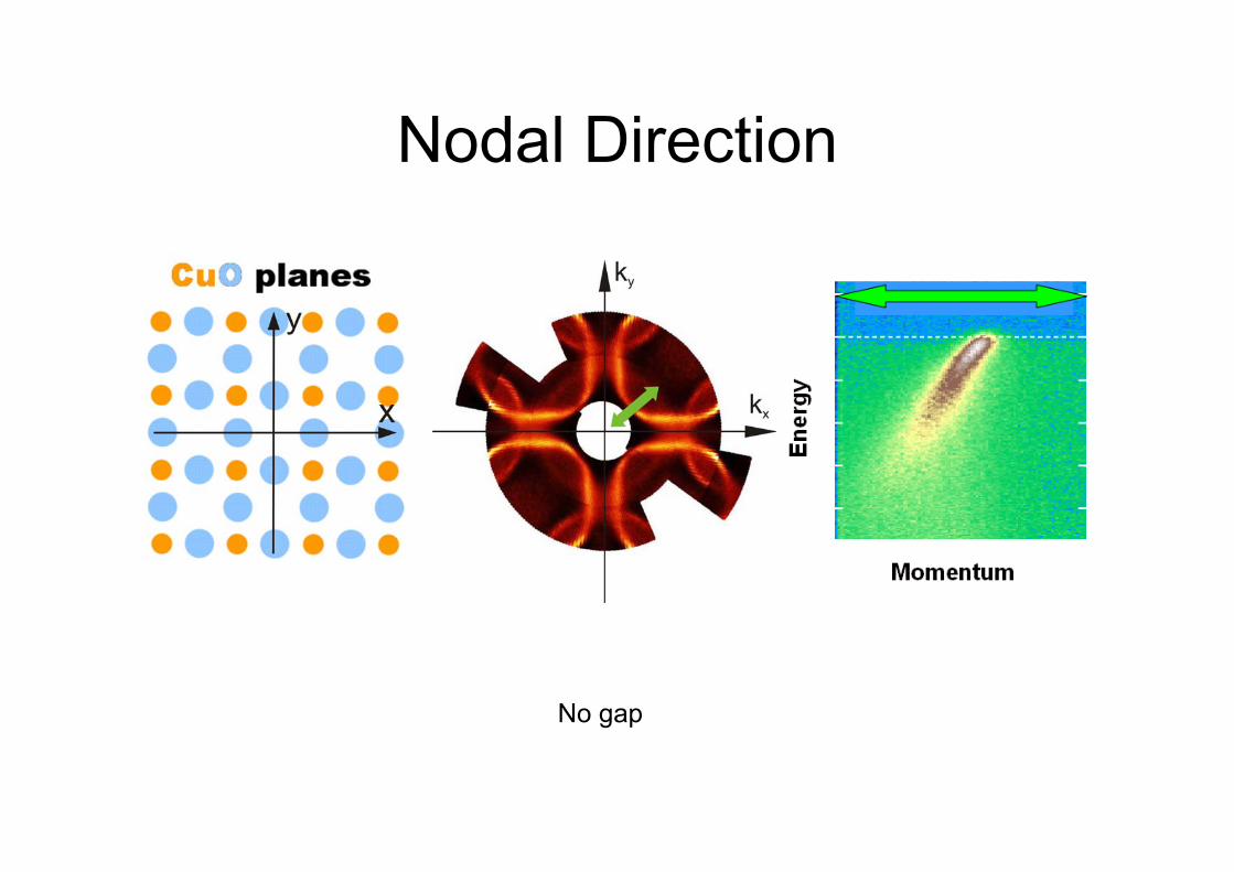
Nodal Direction

No gap

Momentum Resolution

( )( ) 20

2max

00 ))((

)(1),()(ω

ωπ

ωΣ ′′+−⋅

Σ ′′⋅−==

kkvkAkL

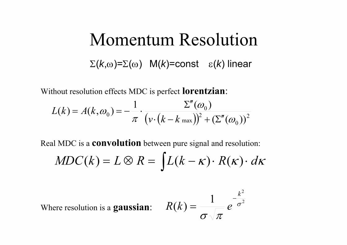
Without resolution effects MDC is perfect lorentzian:

Real MDC is a convolution between pure signal and resolution:

κκκ dRkLRLkMDC ⋅⋅−=⊗= ∫ )()()(

2

2

1)( σ

πσ

k

ekR−

=Where resolution is a gaussian:

Σ(k,ω)=Σ(ω) M(k)=const ε(k) linear

Real MDC = Pure MDC(Lorentzian)

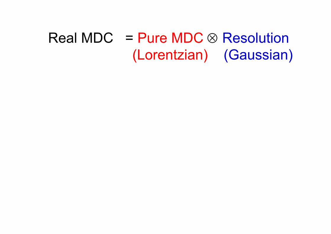
Real MDC = Pure MDC ⊗ Resolution(Lorentzian) (Gaussian)

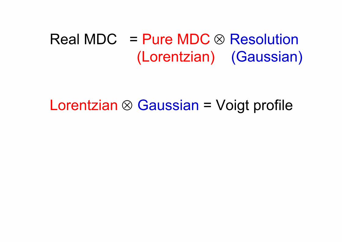
Lorentzian ⊗ Gaussian = Voigt profile


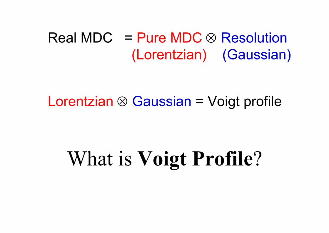
What is Voigt Profile?

Lorentzian ⊗ Gaussian = Voigt profile


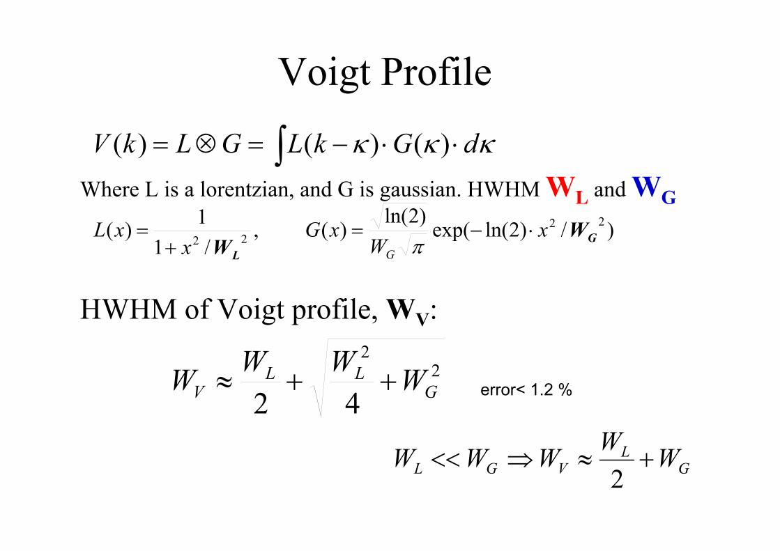
Voigt Profile

κκκ dGkLGLkV ⋅⋅−=⊗= ∫ )()()(

42

22

GLL

V WWWW ++≈

Where L is a lorentzian, and G is gaussian. HWHM WL and WG

)/)2ln(exp()2ln(

)( ,/1

1)( 2222 G

L

WW

xW

xGx

xLG

⋅−=+

=π

HWHM of Voigt profile, WV:

GL

VGL WWWWW +≈⇒<<2

error< 1.2 %

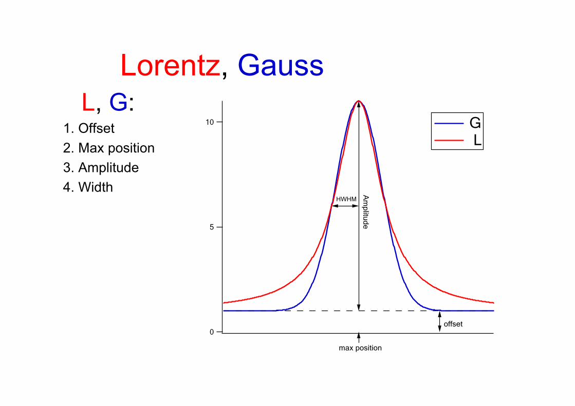
L, G:1. Offset2. Max position3. Amplitude4. Width

Lorentz, Gauss10

5

0

HWHM

Am

plitude

max position

offset

G L

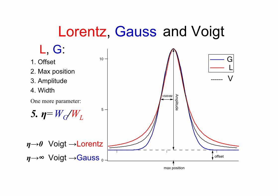
and VoigtL, G:

1. Offset2. Max position3. Amplitude4. Width

Lorentz, Gauss

One more parameter:

5. η=WG/WL

10

5

0

HWHM

Am

plitude

max position

offset

G L

------ V

Voigt →Lorentz

η→∞

η→0

Voigt →Gauss

0.500.400.30k, 1/A

-0.4

-0.2

0.0

ω, eV

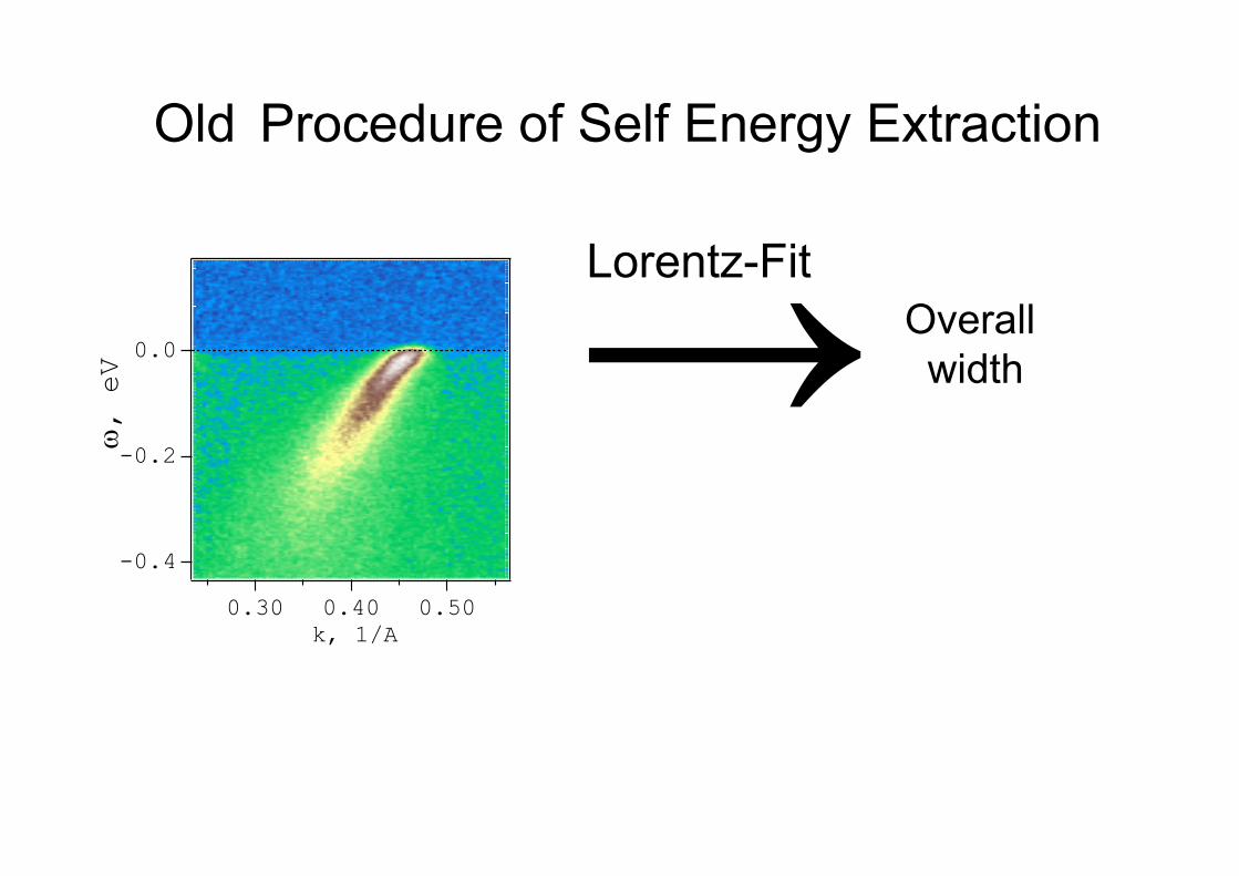
Old

Lorentz-FitOverall width

Procedure of Self Energy Extraction

0.500.400.30k, 1/A

-0.4

-0.2

0.0

ω, eV

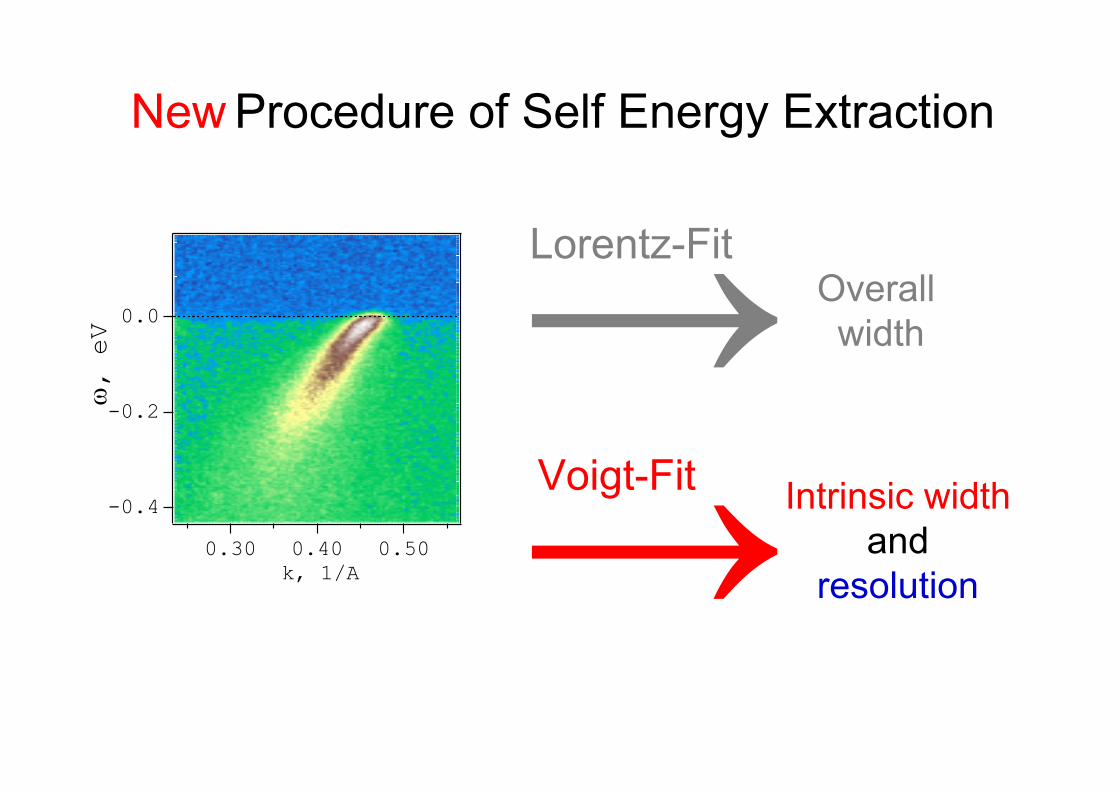
New

Voigt-Fit

Lorentz-FitOverall width

Intrinsic widthand

resolution

Procedure of Self Energy Extraction

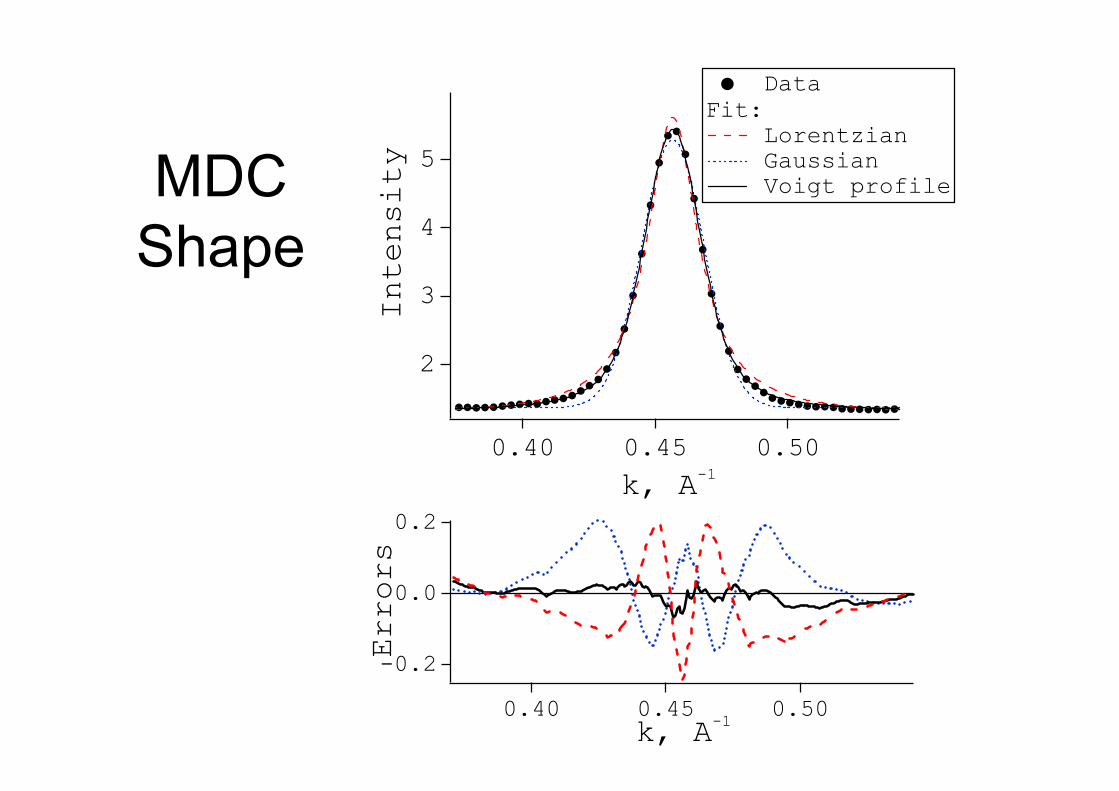
MDC Shape

-0.2

0.0

0.2

Errors

0.500.450.40k, A-1

5

4

3

2Intensity

0.500.450.40

k, A-1

DataFit:

Lorentzian Gaussian Voigt profile

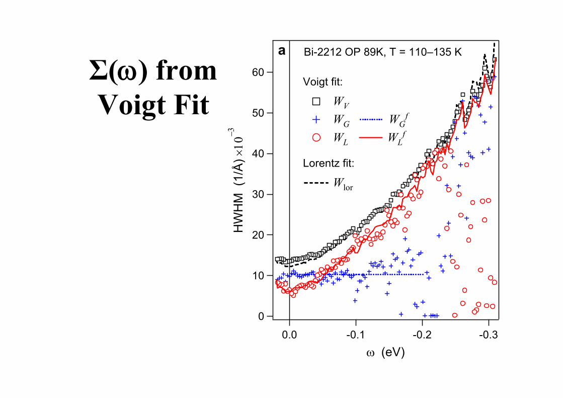
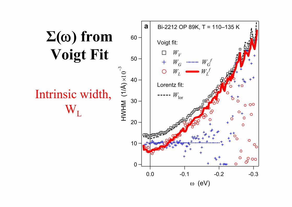
Σ(ω) from Voigt Fit

60

50

40

30

20

10

0

HW

HM

(1/

Å) ×

10−3

-0.3-0.2-0.10.0ω (eV)

Voigt fit:

WV

WG WGf

WL WLf

Lorentz fit:

Wlor

Bi-2212 OP 89K, T = 110–135 Ka


60

50

40

30

20

10

0

HW

HM

(1/

Å) ×

10−3

-0.3-0.2-0.10.0ω (eV)

Voigt fit:

WV

WG WGf

WL WLf

Lorentz fit:

Wlor

Bi-2212 OP 89K, T = 110–135 Ka

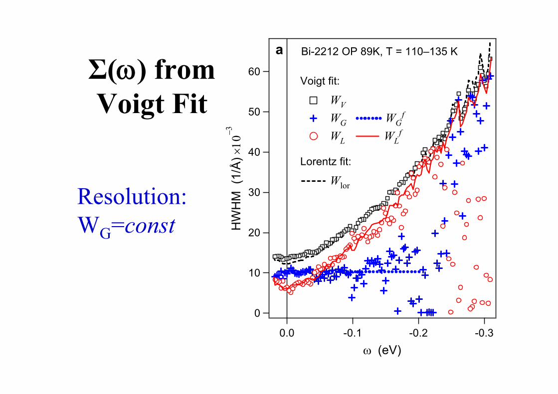
Resolution:WG=const


60

50

40

30

20

10

0

HW

HM

(1/

Å) ×

10−3

-0.3-0.2-0.10.0ω (eV)

Voigt fit:

WV

WG WGf

WL WLf

Lorentz fit:

Wlor

Bi-2212 OP 89K, T = 110–135 Ka

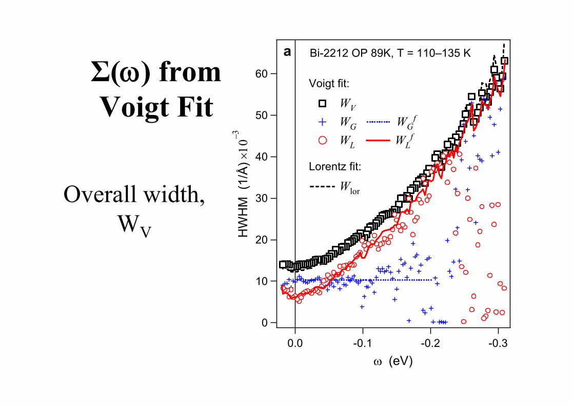
Overall width,WV


60

50

40

30

20

10

0

HW

HM

(1/

Å) ×

10−3

-0.3-0.2-0.10.0ω (eV)

Voigt fit:

WV

WG WGf

WL WLf

Lorentz fit:

Wlor

Bi-2212 OP 89K, T = 110–135 Ka

Intrinsic width,WL

Examples of Voigt fit Application to ARPES Data

• BSCCO• x=0.21• x=0.16• x=0.12

• YBCO• Temperature dependence• Comparison to high-resolution data

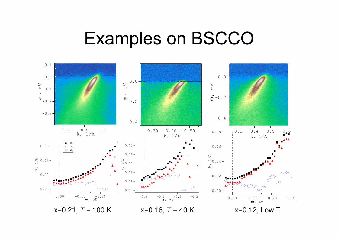
Examples on BSCCO

0.06

0.04

0.02

0.00

W, 1/A

-0.20-0.100.00ω, эВ

WV WL WG

0.05

0.04

0.03

0.02

0.01

0.00

W, 1/A

-0.3-0.2-0.10.0ω, eV

0.08

0.06

0.04

0.02

0.00

W, 1/A

-0.30-0.20-0.100.00 ω, eV

0.50.40.3k, 1/A

-0.3

-0.2

-0.1

0.0

0.1

ω , eV

0.500.400.30k, 1/A

-0.4

-0.2

0.0

ω, eV

0.60.50.40.3k, 1/A

-0.4

-0.2

0.0

ω, eV

x=0.21, T = 100 K x=0.16, T = 40 K x=0.12, Low T

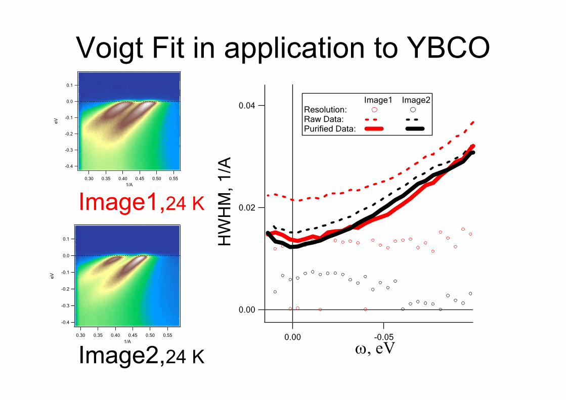
Voigt Fit in application to YBCO

0.550.500.450.400.350.301/A

-0.4

-0.3

-0.2

-0.1

0.0

0.1

eV

0.550.500.450.400.350.301/A

-0.4

-0.3

-0.2

-0.1

0.0

0.1

eV

0.04

0.02

0.00

HW

HM

, 1/A

-0.050.00

ω, eV

Image1 Image2Resolution: Raw Data: Purified Data:

Image1,24 K

Image2,24 K

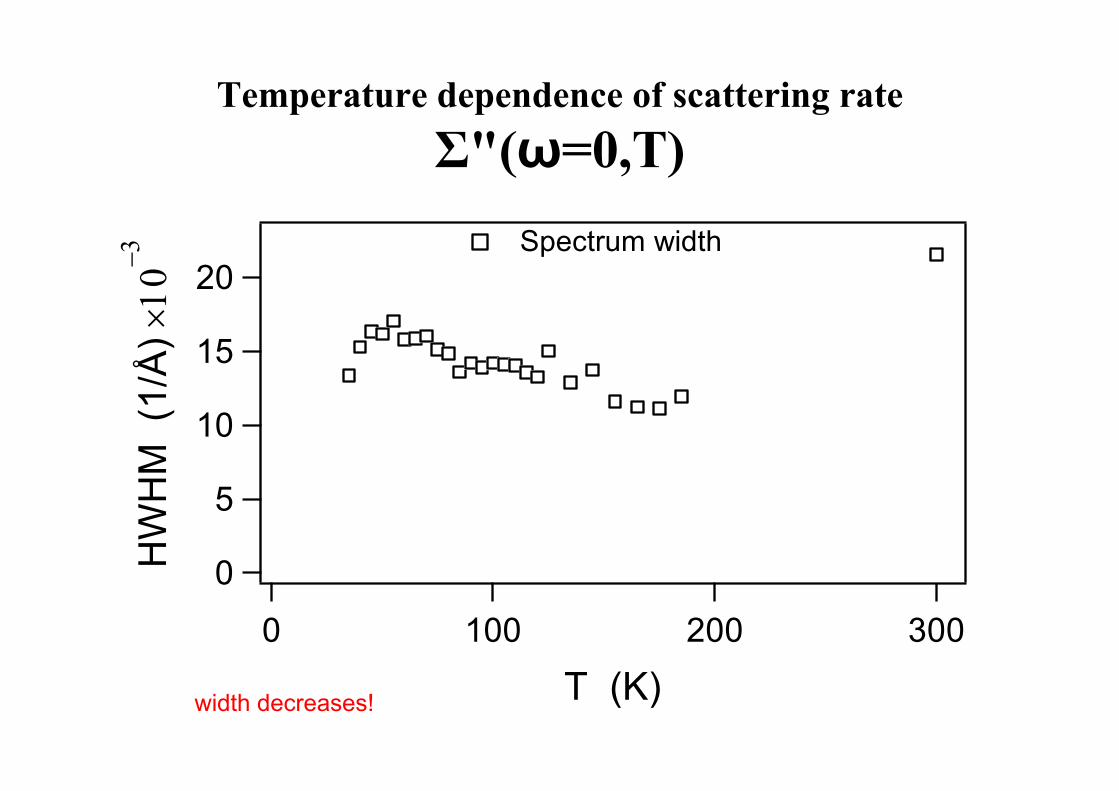
Temperature dependence of scattering rate Σ"(ω=0,T)

20

15

10

5

0HW

HM

(1/

Å) ×

10−3

3002001000

T (K)

Spectrum width

width decreases!

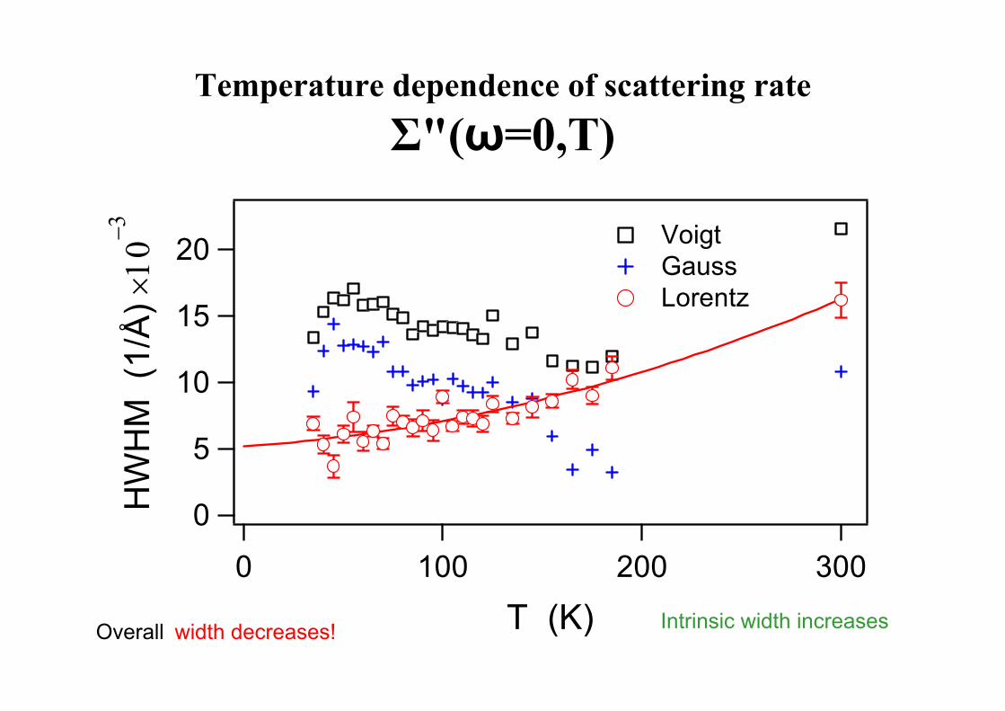
Temperature dependence of scattering rate Σ"(ω=0,T)

20

15

10

5

0HW

HM

(1/

Å) ×

10−3

3002001000

T (K)

Voigt Gauss Lorentz

width decreases!Overall Intrinsic width increases

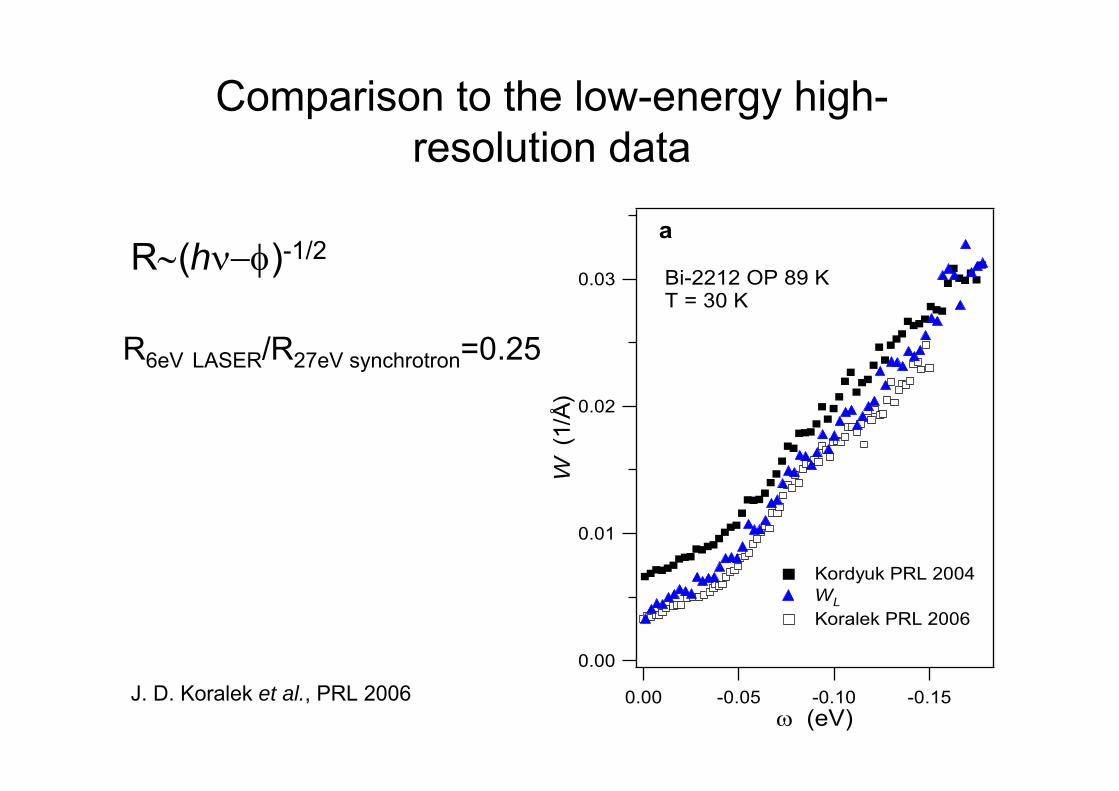
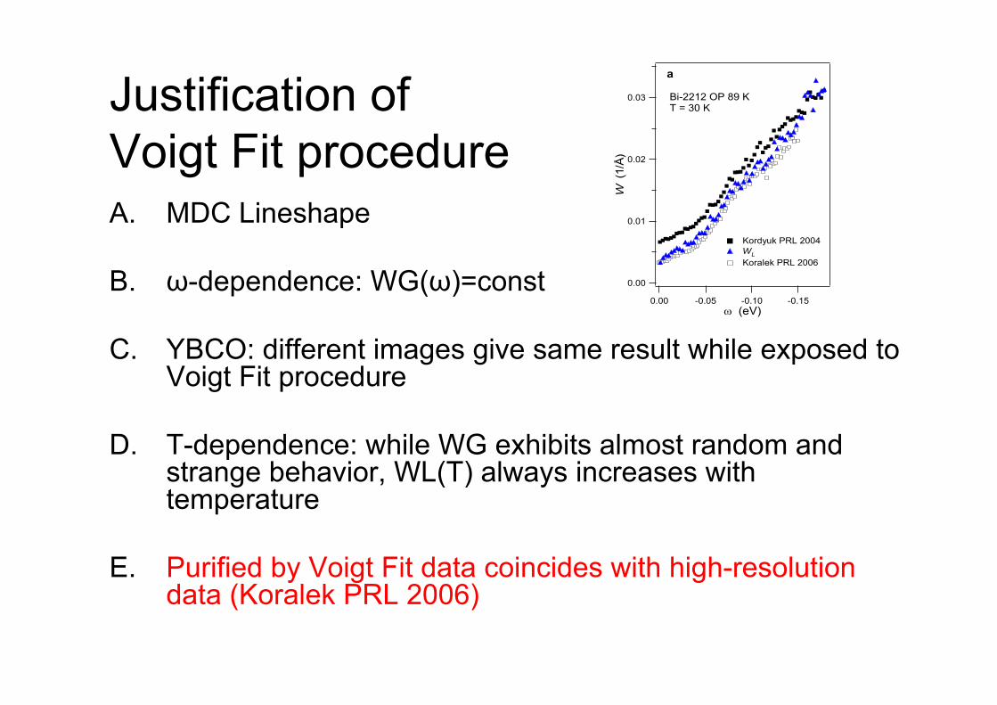
Comparison to the low-energy high-resolution data

0.03

0.02

0.01

0.00

W (

1/Å)

-0.15-0.10-0.050.00ω (eV)

Kordyuk PRL 2004 WL Koralek PRL 2006

a

Bi-2212 OP 89 KT = 30 K

J. D. Koralek et al., PRL 2006

R∼(hν−φ)-1/2

R6eV LASER/R27eV synchrotron=0.25

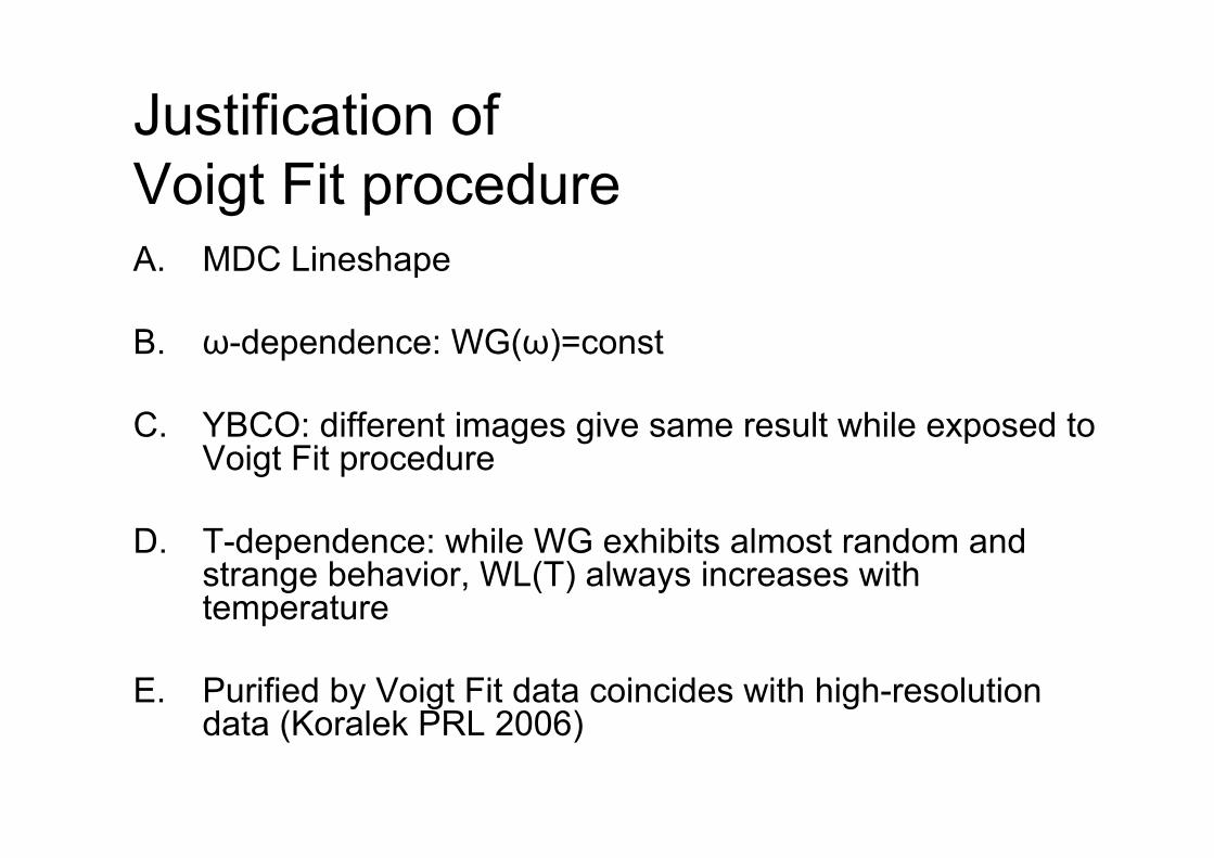
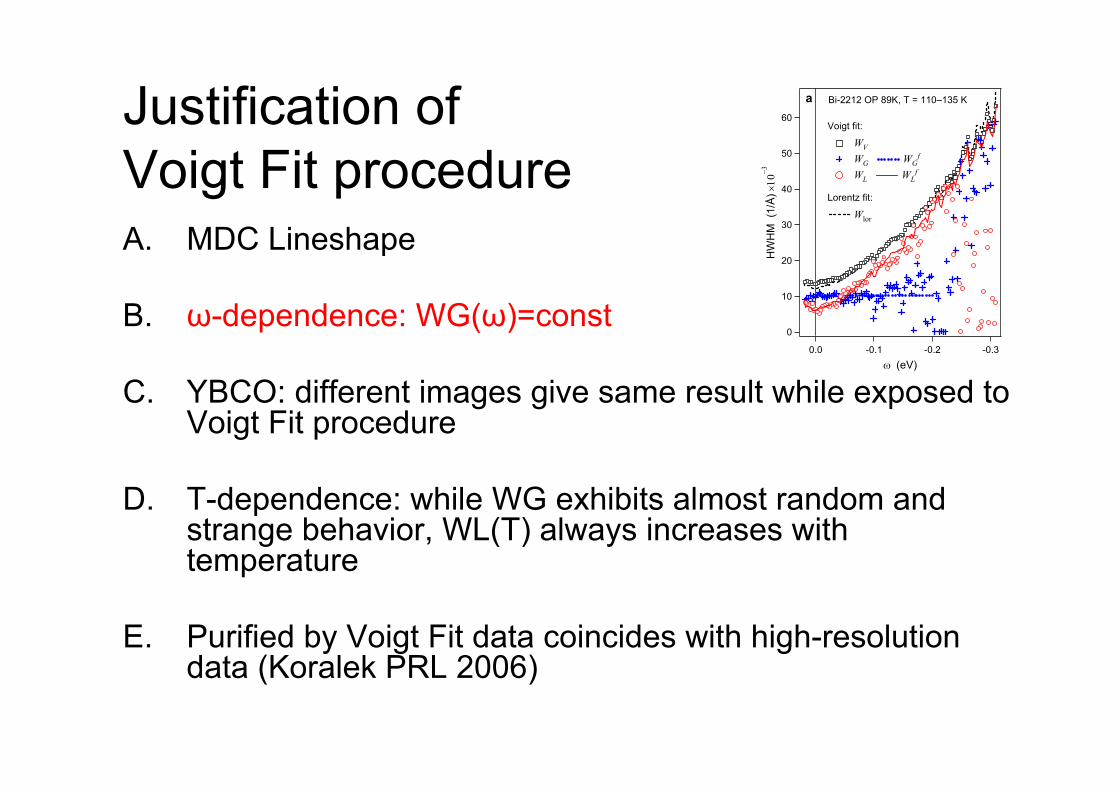
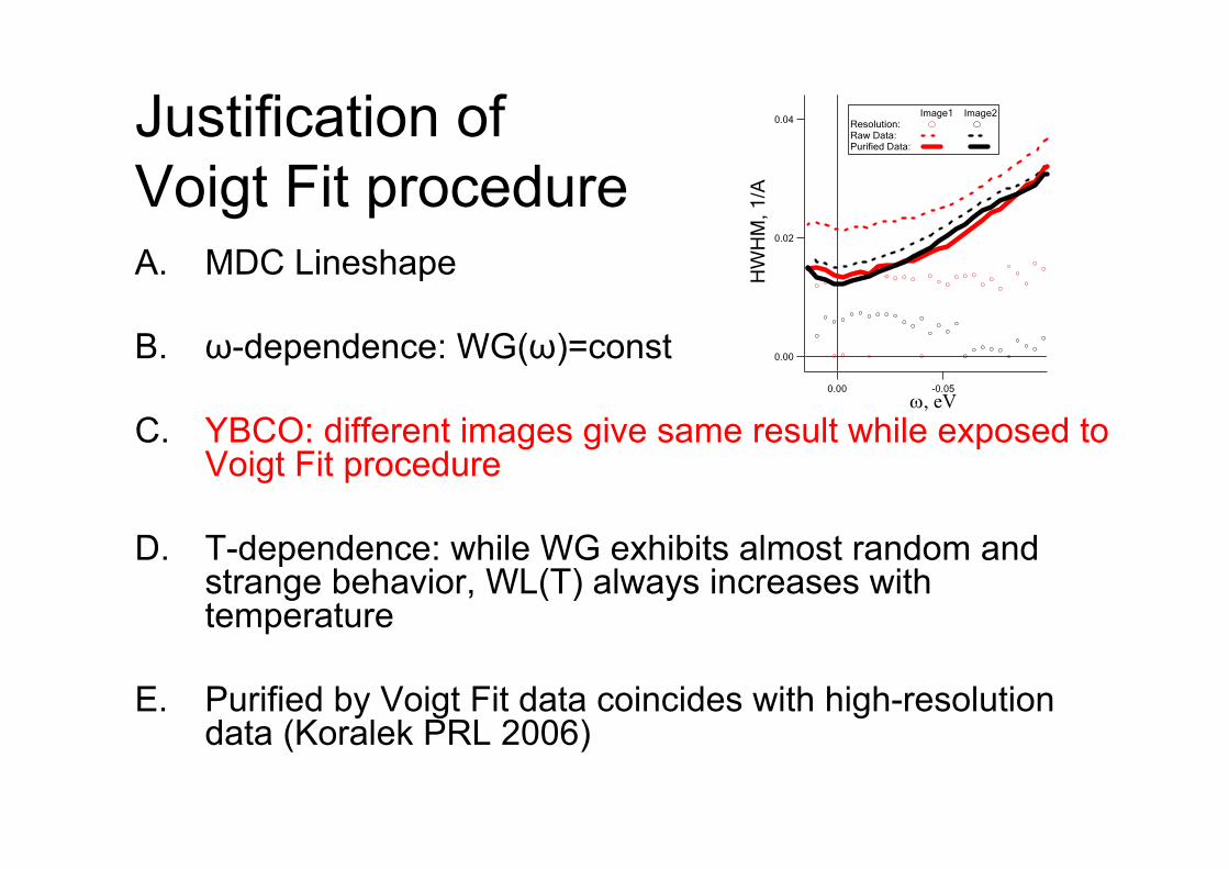
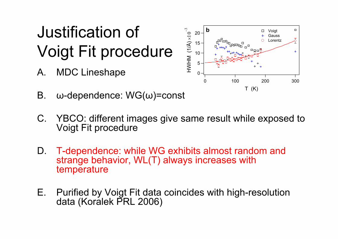
Justification of Voigt Fit procedureA. MDC Lineshape

B. ω-dependence: WG(ω)=const

C. YBCO: different images give same result while exposed to Voigt Fit procedure

D. T-dependence: while WG exhibits almost random and strange behavior, WL(T) always increases with temperature

E. Purified by Voigt Fit data coincides with high-resolution data (Koralek PRL 2006)

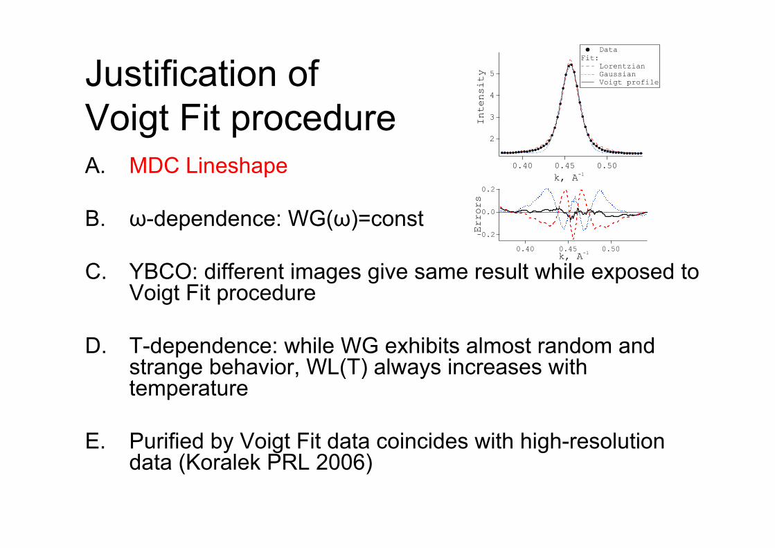
Justification of Voigt Fit procedure

-0.2

0.0

0.2

Errors

0.500.450.40k, A-1

5

4

3

2

Intensity

0.500.450.40

k, A-1

DataFit:

Lorentzian Gaussian Voigt profile

A. MDC Lineshape






60

50

40

30

20

10

0

HW

HM

(1/

Å) ×

10−3

-0.3-0.2-0.10.0ω (eV)

Voigt fit:

WV

WG WGf

WL WLf

Lorentz fit:

Wlor

Bi-2212 OP 89K, T = 110–135 Ka

A. MDC Lineshape






0.04

0.02

0.00

HW

HM

, 1/A

-0.050.00

ω, eV

Image1 Image2Resolution: Raw Data: Purified Data:

A. MDC Lineshape






20

15

10

5

0HW

HM

(1/

Å) ×

10−3

3002001000

T (K)

Voigt Gauss Lorentz

b

A. MDC Lineshape






0.03

0.02

0.01

0.00

W (

1/Å)

-0.15-0.10-0.050.00ω (eV)

Kordyuk PRL 2004 WL Koralek PRL 2006

a

Bi-2212 OP 89 KT = 30 K

A. MDC Lineshape





Most interesting part ☺

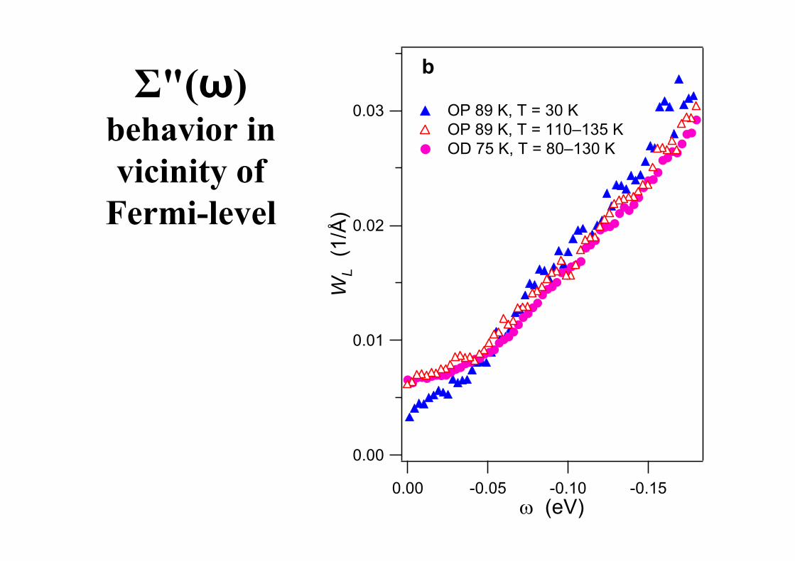
Σ"(ω) behavior in vicinity of

Fermi-level

0.03

0.02

0.01

0.00

WL

(1/Å

)

-0.15-0.10-0.050.00ω (eV)

OP 89 K, T = 30 K OP 89 K, T = 110–135 K OD 75 K, T = 80–130 K

b

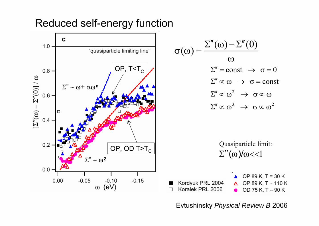
ωΣ ′′−ωΣ ′′

=ωσ)0()()(

23

2

const 0 const

ω∝σ→ω∝Σ ′′

ω∝σ→ω∝Σ ′′

=σ→ω∝Σ ′′=σ→=Σ ′′

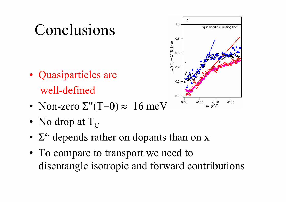
Reduced self-energy function

Evtushinsky Physical Review B 2006

Quasiparticle limit:Σ’’(ω)/ω<<1

Σ” ∼ ω2

Σ” ∼ ω+ αωn

OP, T<TC

OP, OD T>TC

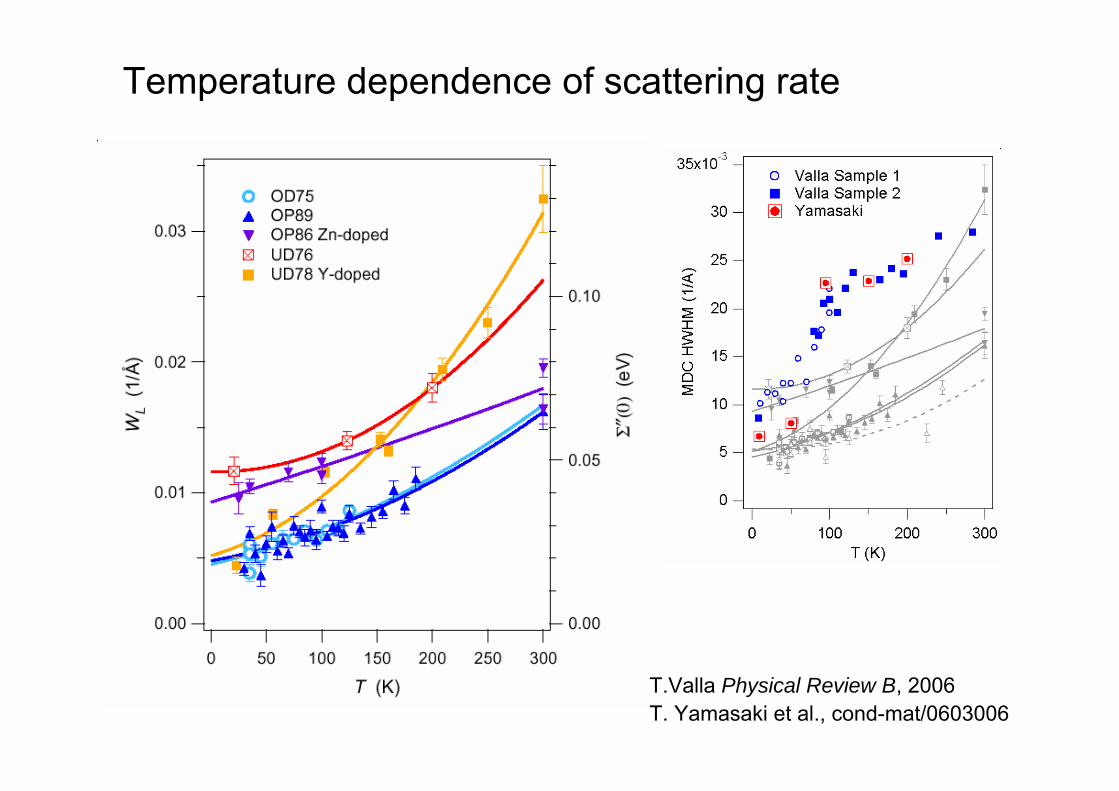
Temperature dependence of scattering rate

T.Valla Physical Review B, 2006T. Yamasaki et al., cond-mat/0603006

ARPESvs.

Transport

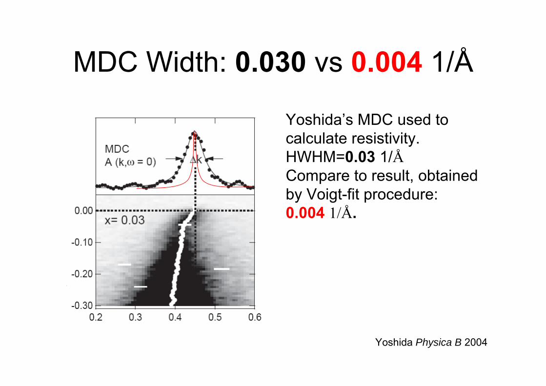
MDC Width: 0.030 vs 0.004 1/Å

Yoshida’s MDC used to calculate resistivity. HWHM=0.03 1/ÅCompare to result, obtainedby Voigt-fit procedure: 0.004 1/Å.

Yoshida Physica B 2004

r

imF

vnek

nem Σ ′′

≈τ

=ρη220

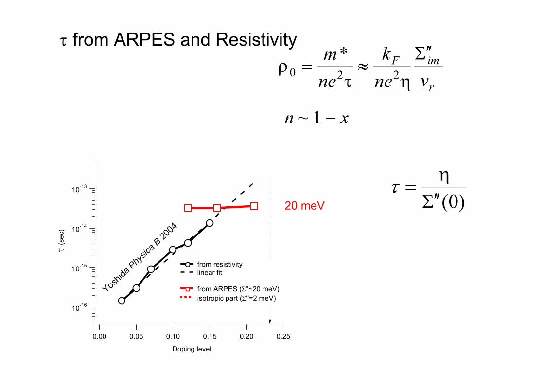
*τ from ARPES and Resistivity

Yoshid

a Physic

a B 2004

10-16

10-15

10-14

10-13

τ (s

ec)

0.250.200.150.100.050.00

Doping level

from resistivity linear fit

from ARPES (Σ''~20 meV) isotropic part (Σ''=2 meV)

20 meV

n ~ 1 − x

)0(Σ ′′=

ητ

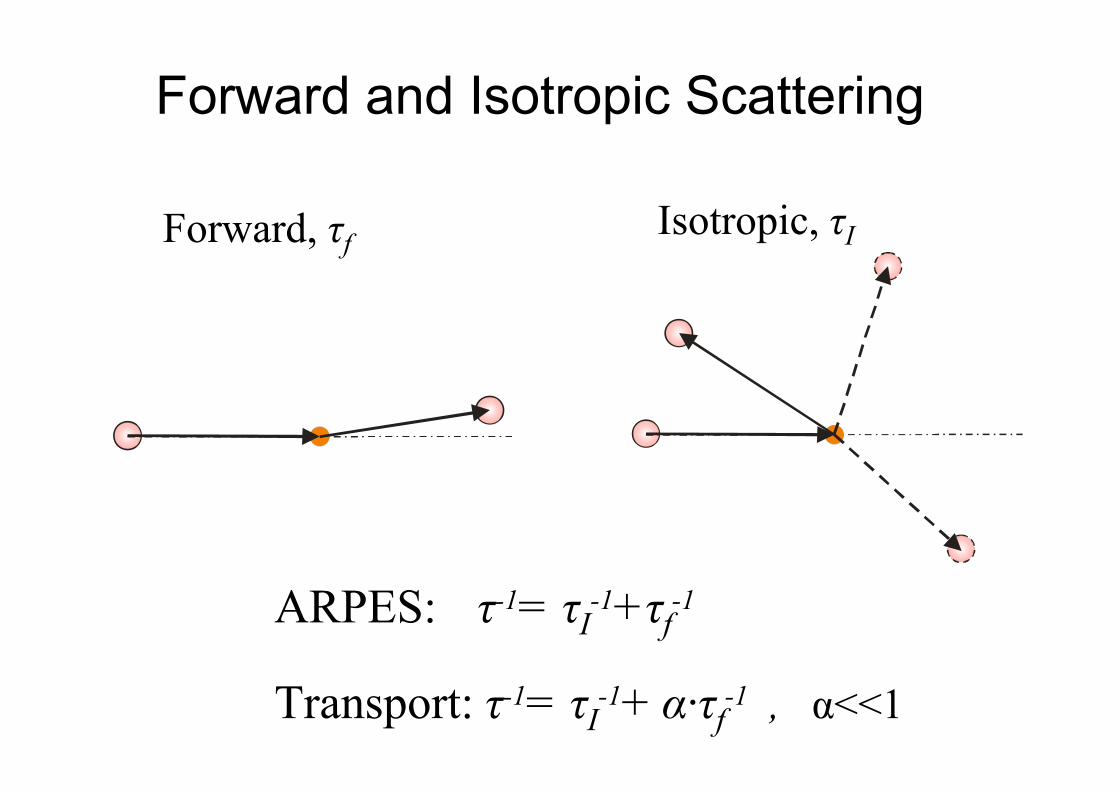
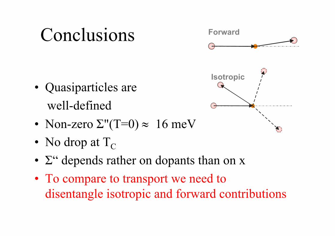
Forward and Isotropic Scattering

Forward, τf Isotropic, τI

Transport: τ-1= τI-1+ α·τf-1 , α<<1

ARPES: τ-1= τI-1+τf-1

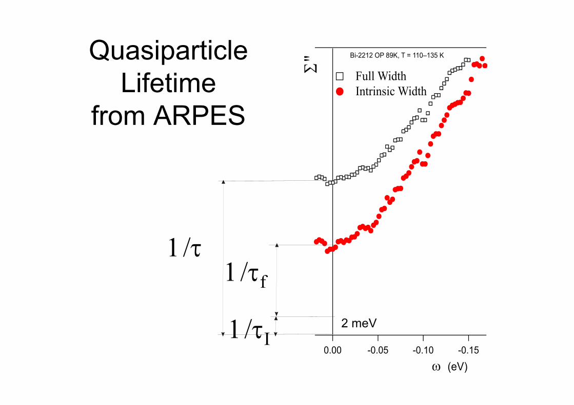
Quasiparticle Lifetime

from ARPES

1/τf

1/τI

1/τ

Σ"

-0.15-0.10-0.050.00

ω (eV)

Full Width Intrinsic Width

Bi-2212 OP 89K, T = 110–135 K

2 meV

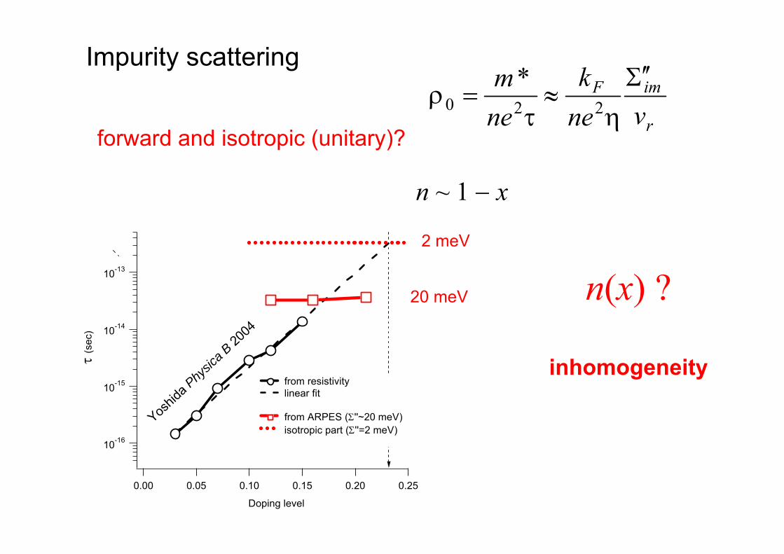
r

imF

vnek

nem Σ ′′

≈τ

=ρη220

*Impurity scattering

Yoshid

a Physic

a B 2004

n(x) ?

inhomogeneity

forward and isotropic (unitary)?

10-16

10-15

10-14

10-13

τ (s

ec)

0.250.200.150.100.050.00

Doping level

from resistivity linear fit

from ARPES (Σ''~20 meV) isotropic part (Σ''=2 meV)

20 meV

2 meV

n ~ 1 − x

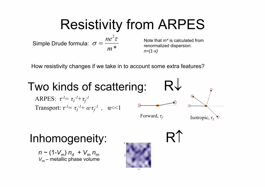
Resistivity from ARPES*

2

mne τσ =Simple Drude formula: Note that m* is calculated from

renormalized dispersion.n=(1-x)

How resistivity changes if we take in to account some extra features?

Two kinds of scattering: R↓ARPES: τ-1= τI-1+τf-1

Transport: τ-1= τI-1+ α·τf-1 , α<<1Forward, τf Isotropic, τI

Inhomogeneity: R↑n ~ (1-Vm) nd + Vm nmVm – metallic phase volume

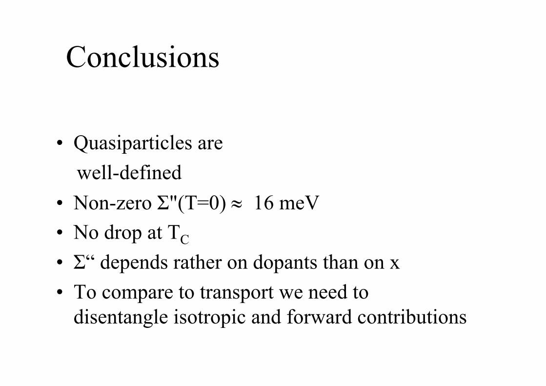
Conclusions

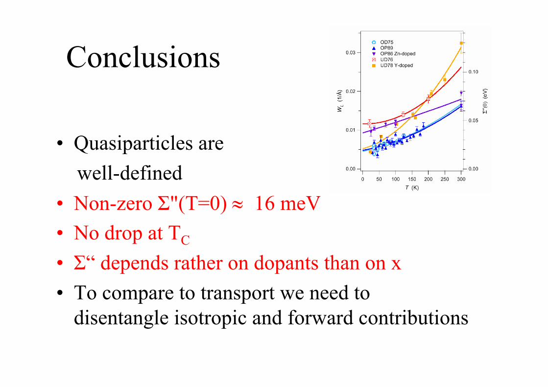
• Quasiparticles are well-defined

• Non-zero Σ"(T=0) ≈ 16 meV• No drop at TC

• Σ“ depends rather on dopants than on x• To compare to transport we need to

disentangle isotropic and forward contributions

Conclusions

• Quasiparticles are well-defined

• Non-zero Σ"(T=0) ≈ 16 meV• No drop at TC

• Σ“ depends rather on dopants than on x• To compare to transport we need to

disentangle isotropic and forward contributions

Forward

Isotropic

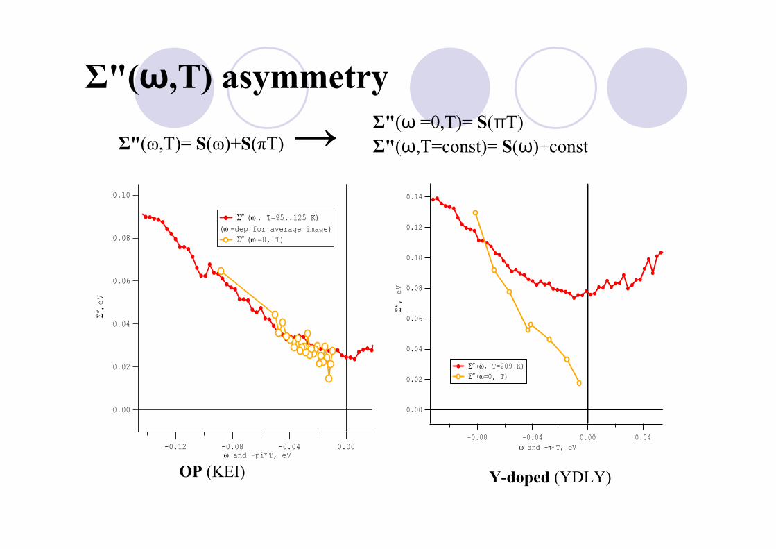
Σ"(ω,T) asymmetryΣ"(ω =0,T)= S(πT)Σ"(ω,T=const)= S(ω)+const

0.10

0.08

0.06

0.04

0.02

0.00

Σ″, e

V

-0.12 -0.08 -0.04 0.00ω and -pi*T, eV

Σ″ (ω , T=95..125 K) (ω -dep for average image)

Σ″ (ω =0, T)

Σ"(ω,T)= S(ω)+S(πT) →0.14

0.12

0.10

0.08

0.06

0.04

0.02

0.00Σ″, eV

-0.08 -0.04 0.00 0.04ω and -π*T, eV

Σ″(ω, T=209 K) Σ″(ω=0, T)

OP (KEI) Y-doped (YDLY)

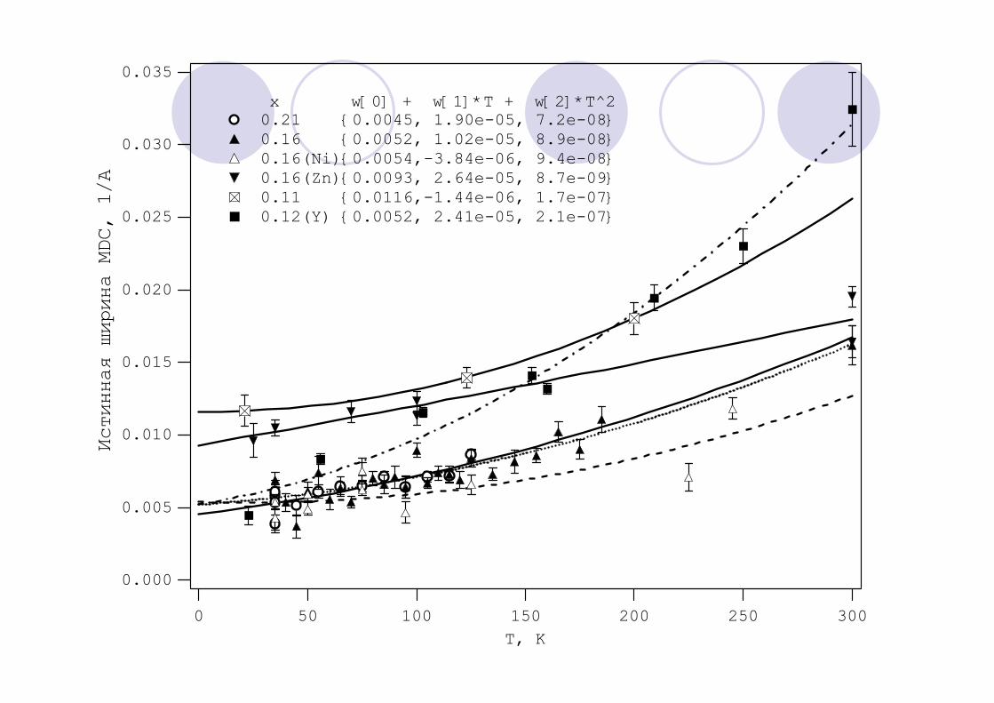
0.035

0.030

0.025

0.020

0.015

0.010

0.005

0.000

Истинная ширина MDC, 1/A

300250200150100500T, K

x w[0] + w[1]*T + w[2]*T^2 0.21 {0.0045, 1.90e-05, 7.2e-08} 0.16 {0.0052, 1.02e-05, 8.9e-08} 0.16(Ni){0.0054,-3.84e-06, 9.4e-08} 0.16(Zn){0.0093, 2.64e-05, 8.7e-09} 0.11 {0.0116,-1.44e-06, 1.7e-07} 0.12(Y) {0.0052, 2.41e-05, 2.1e-07}

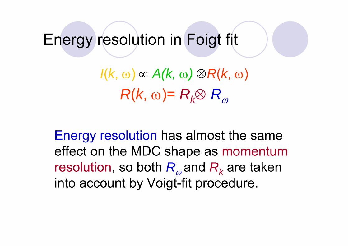
Energy resolution in Foigt fit

I(k, ω) ∝ A(k, ω) ⊗R(k, ω)R(k, ω)= Rk⊗ Rω

Energy resolution has almost the same effect on the MDC shape as momentum resolution, so both Rω and Rk are taken into account by Voigt-fit procedure.

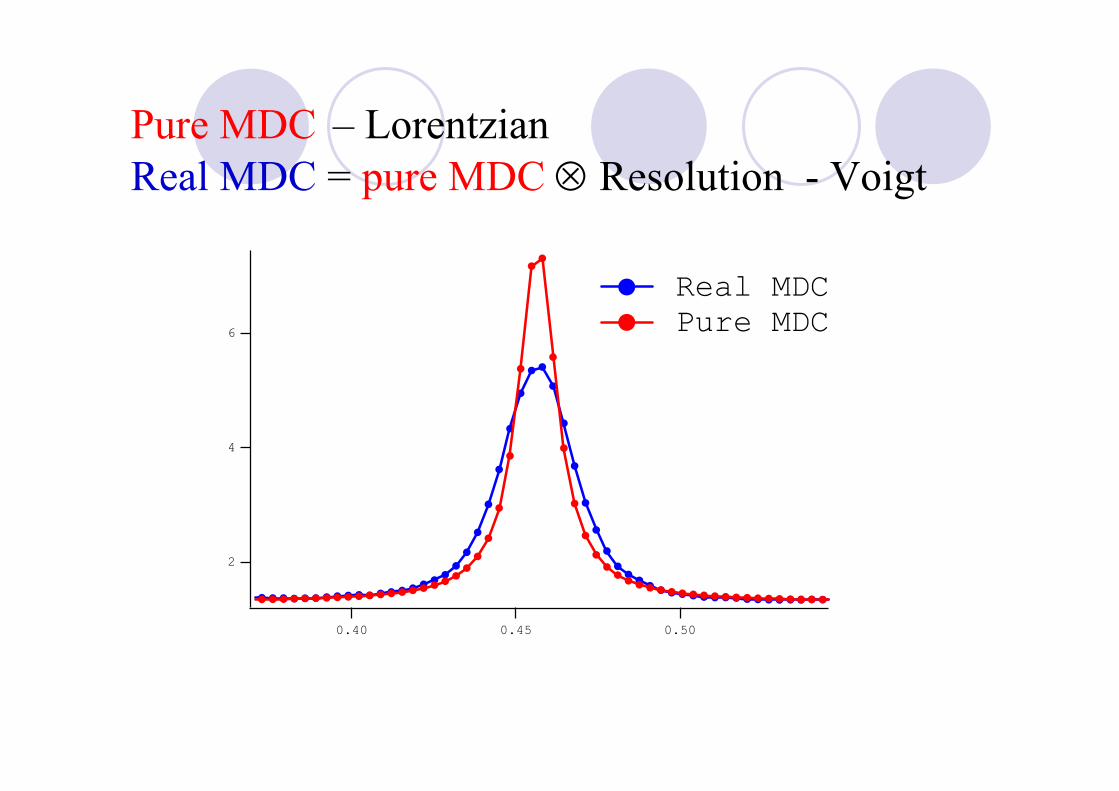
Pure MDC – LorentzianReal MDC = pure MDC ⊗ Resolution - Voigt

6

4

2

0.500.450.40

Real MDC Pure MDC

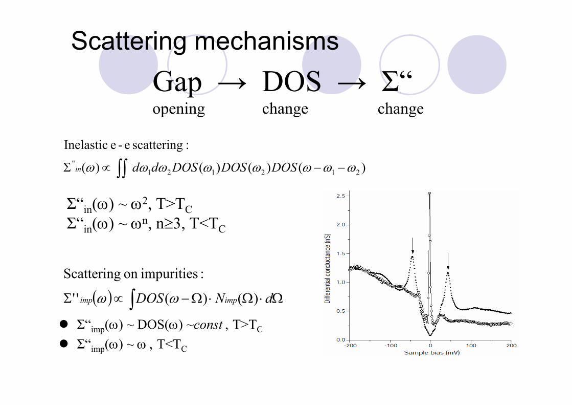
Scattering mechanisms

Σ“imp(ω) ~ DOS(ω) ~const , T>TC

Σ“imp(ω) ~ ω , T<TC

Gap → DOS → Σ“opening change change

)()()()(

:scattering e-e Inelastic

212121'' ωωωωωωωω −−∝Σ ∫∫ DOSDOSDOSddin

Σ“in(ω) ~ ω2, T>TCΣ“in(ω) ~ ωn, n≥3, T<TC

( ) Ω⋅Ω⋅Ω−∝Σ ∫ dNDOS impimp )()(''

:impuritieson Scattering

ωω

Unadulterated spectral function of low-energy quasiparticles

Documents

Transcript of Unadulterated spectral function of low-energy quasiparticles