Physics-based preconditioning of sound wavesA Jacobian-free Newton-Krylov method for implicit multi-D

hydrodynamics

Maxime VialletMax-Planck-Institute für Astrophysik, Garching

Workshop on Newton-Krylov methodsLyon, October 6th, 2013

Max-Planck-Institut für Astrophysik

Outline

• Introduction

• Newton-Krylov solvers

• Conclusion

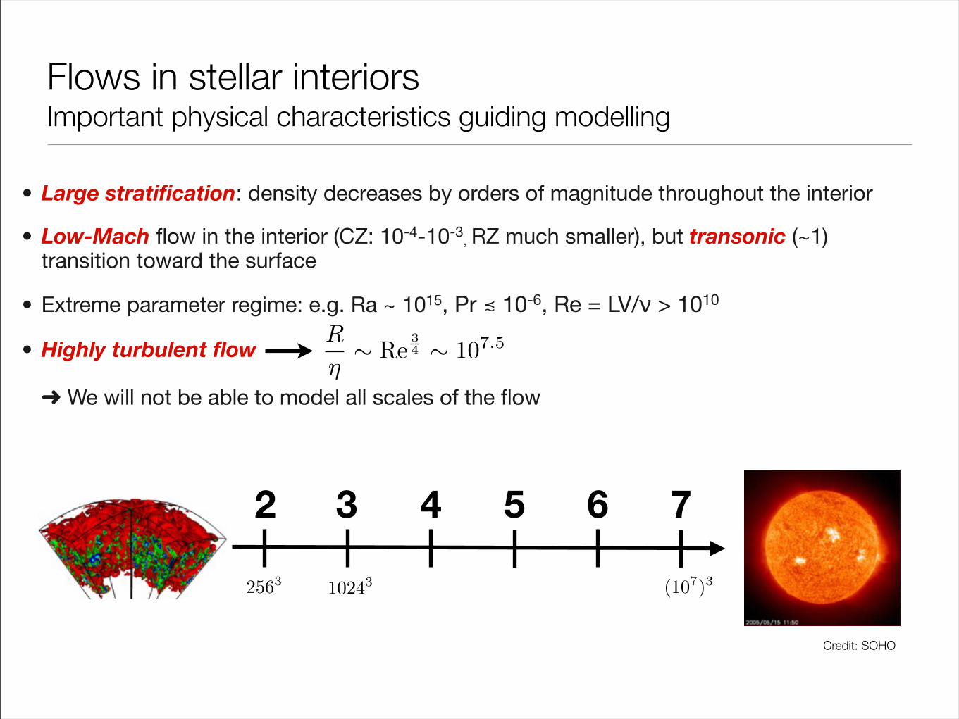
Flows in stellar interiorsImportant physical characteristics guiding modelling

• Large stratification: density decreases by orders of magnitude throughout the interior

• Low-Mach flow in the interior (CZ: 10-4-10-3, RZ much smaller), but transonic (~1) transition toward the surface

• Extreme parameter regime: e.g. Ra ~ 1015, Pr ≾ 10-6, Re = LV/ν > 1010

• Highly turbulent flow

! We will not be able to model all scales of the flow

2563 10243

2 3 4 5 6 7

Credit: SOHO

(107)3

R

η∼ Re

34 ∼ 107.5

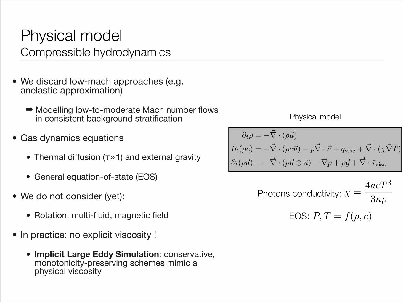
Physical modelCompressible hydrodynamics

• We discard low-mach approaches (e.g. anelastic approximation)

" Modelling low-to-moderate Mach number flows in consistent background stratification

• Gas dynamics equations

• Thermal diffusion (τ≫1) and external gravity

• General equation-of-state (EOS)

• We do not consider (yet):

• Rotation, multi-fluid, magnetic field

• In practice: no explicit viscosity !

• Implicit Large Eddy Simulation: conservative, monotonicity-preserving schemes mimic a physical viscosity

χ =4acT 3

3κρPhotons conductivity:

EOS: P, T = f(ρ, e)

Physical model

∂tρ = −�∇ · (ρ�u)

∂t(ρe) = −�∇ · (ρe�u)− p�∇ · �u+ qvisc + �∇ · (χ�∇T )

∂t(ρ�u) = −�∇ · (ρ�u⊗ �u)− �∇p+ ρ�g + �∇ · ¯̄τvisc

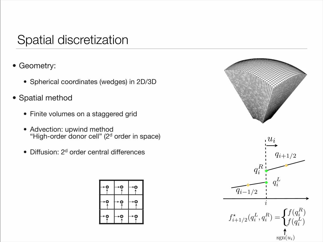
Spatial discretization

• Geometry:

• Spherical coordinates (wedges) in 2D/3D

• Spatial method

• Finite volumes on a staggered grid

• Advection: upwind method “High-order donor cell” (2d order in space)

• Diffusion: 2d order central differences

i

ui

qLi

qRi

qi+1/2

qi−1/2

{sgn(ui)

f(qRi )f(qLi )

f�i+1/2(q

Li , q

Ri ) =

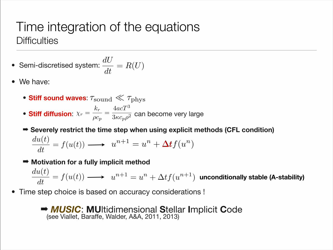
• Semi-discretised system:

• We have:

• Stiff sound waves:

• Stiff diffusion: can become very large

" Severely restrict the time step when using explicit methods (CFL condition)

" Motivation for a fully implicit method

• Time step choice is based on accuracy considerations !

" MUSIC: MUltidimensional Stellar Implicit Code(see Viallet, Baraffe, Walder, A&A, 2011, 2013)

χr =krρcp

=4acT 3

3κcpρ2

Time integration of the equationsDifficulties

τsound � τphys

dU

dt= R(U)

unconditionally stable (A-stability) un+1 = un +∆tf(un+1)du(t)

dt= f(u(t))

du(t)

dt= f(u(t)) un+1 = un +∆tf(un)∆t

Outline

• Introduction

• Newton-Krylov solvers

• Conclusion

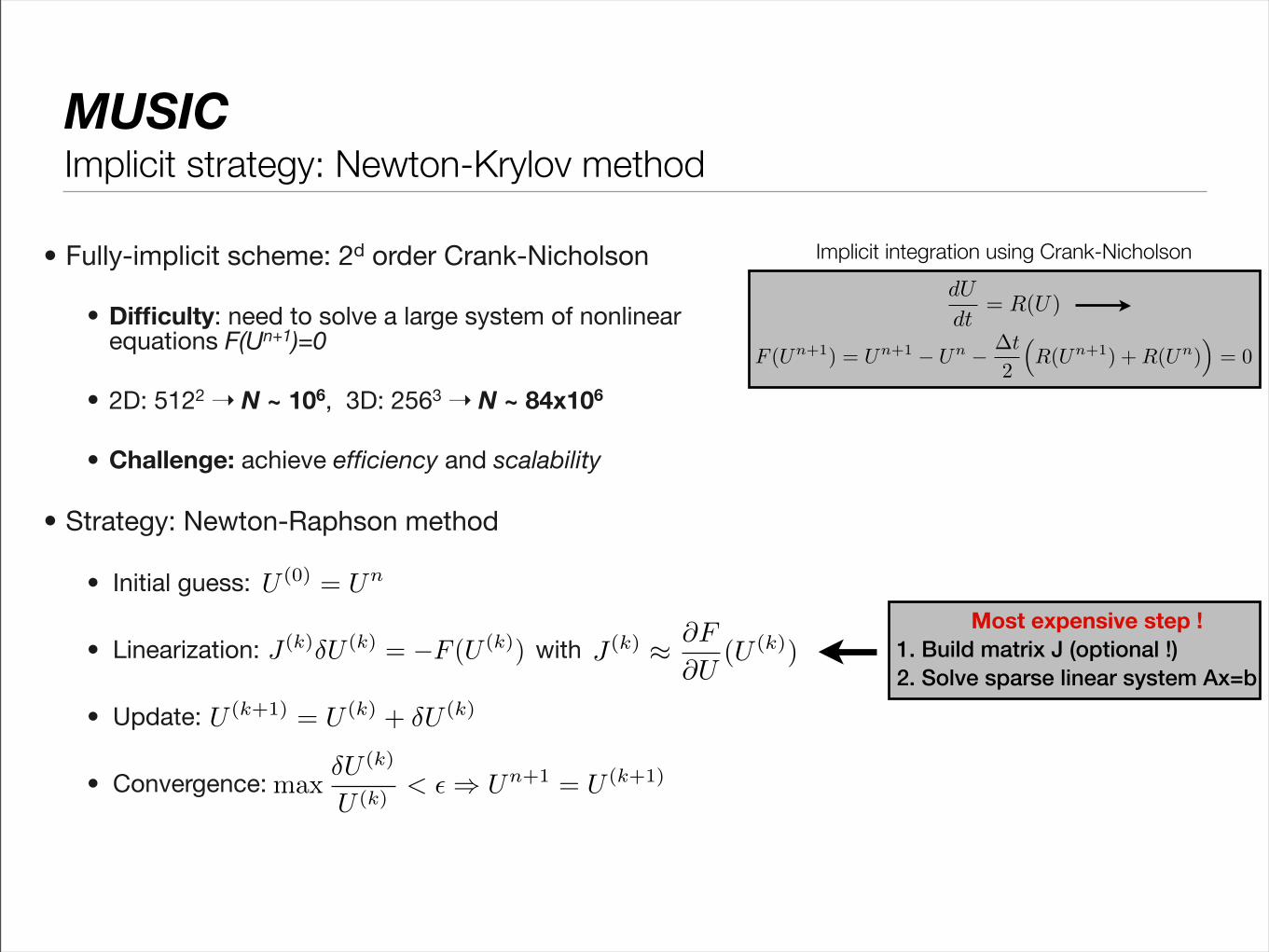
• Fully-implicit scheme: 2d order Crank-Nicholson

• Difficulty: need to solve a large system of nonlinear equations F(Un+1)=0

• 2D: 5122 ! N ~ 106, 3D: 2563 ! N ~ 84x106

• Challenge: achieve efficiency and scalability

• Strategy: Newton-Raphson method

• Initial guess:

• Linearization: with

• Update:

• Convergence:

dU

dt= R(U)

F (Un+1) = Un+1 − Un − ∆t

2

�R(Un+1) +R(Un)

�= 0

Implicit integration using Crank-Nicholson

U (0) = Un

U (k+1) = U (k) + δU (k)

maxδU (k)

U (k)< � ⇒ Un+1 = U (k+1)

J (k)δU (k) = −F (U (k)) J (k) ≈ ∂F

∂U(U (k))

MUSICImplicit strategy: Newton-Krylov method

Most expensive step !1. Build matrix J (optional !)2. Solve sparse linear system Ax=b

MUSICNewton-Krylov method

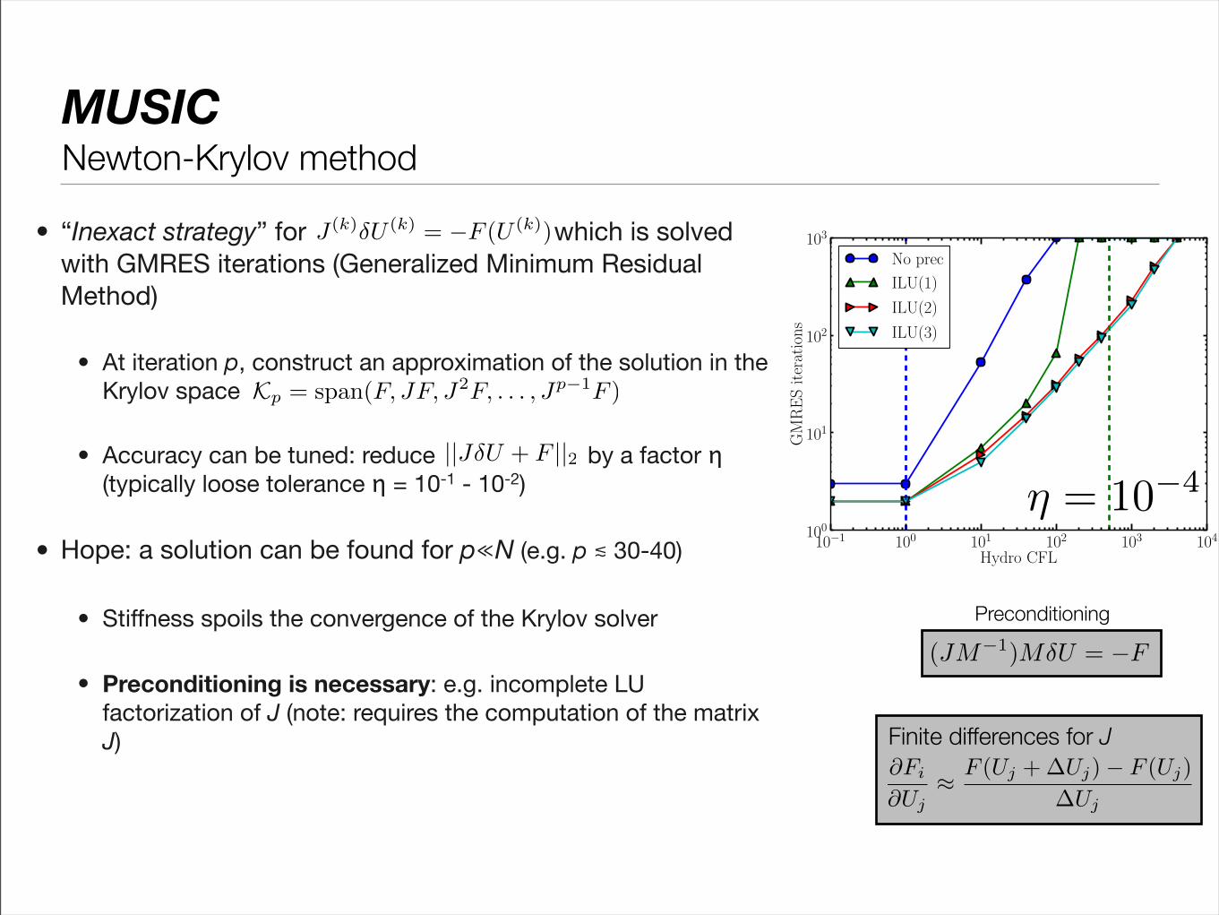
• “Inexact strategy” for which is solved with GMRES iterations (Generalized Minimum Residual Method)

• At iteration p, construct an approximation of the solution in the Krylov space

• Accuracy can be tuned: reduce by a factor η(typically loose tolerance η = 10-1 - 10-2)

• Hope: a solution can be found for p≪N (e.g. p ≲ 30-40)

• Stiffness spoils the convergence of the Krylov solver

• Preconditioning is necessary: e.g. incomplete LU factorization of J (note: requires the computation of the matrix J)

J (k)δU (k) = −F (U (k))

Kp = span(F, JF, J2F, . . . , Jp−1F )

∂Fi

∂Uj≈ F (Uj + ∆Uj)− F (Uj)

∆Uj

Finite differences for J

(JM−1)MδU = −F

Preconditioning

||JδU + F ||2

η = 10−4

104

105

106

107

DOFs

10−1

100

101

102

103

Tim

e(s)

∝ N

163

323

643

1282

2562

5122

10242

Jacobian

ILU(2)

GMRES (20 iters)

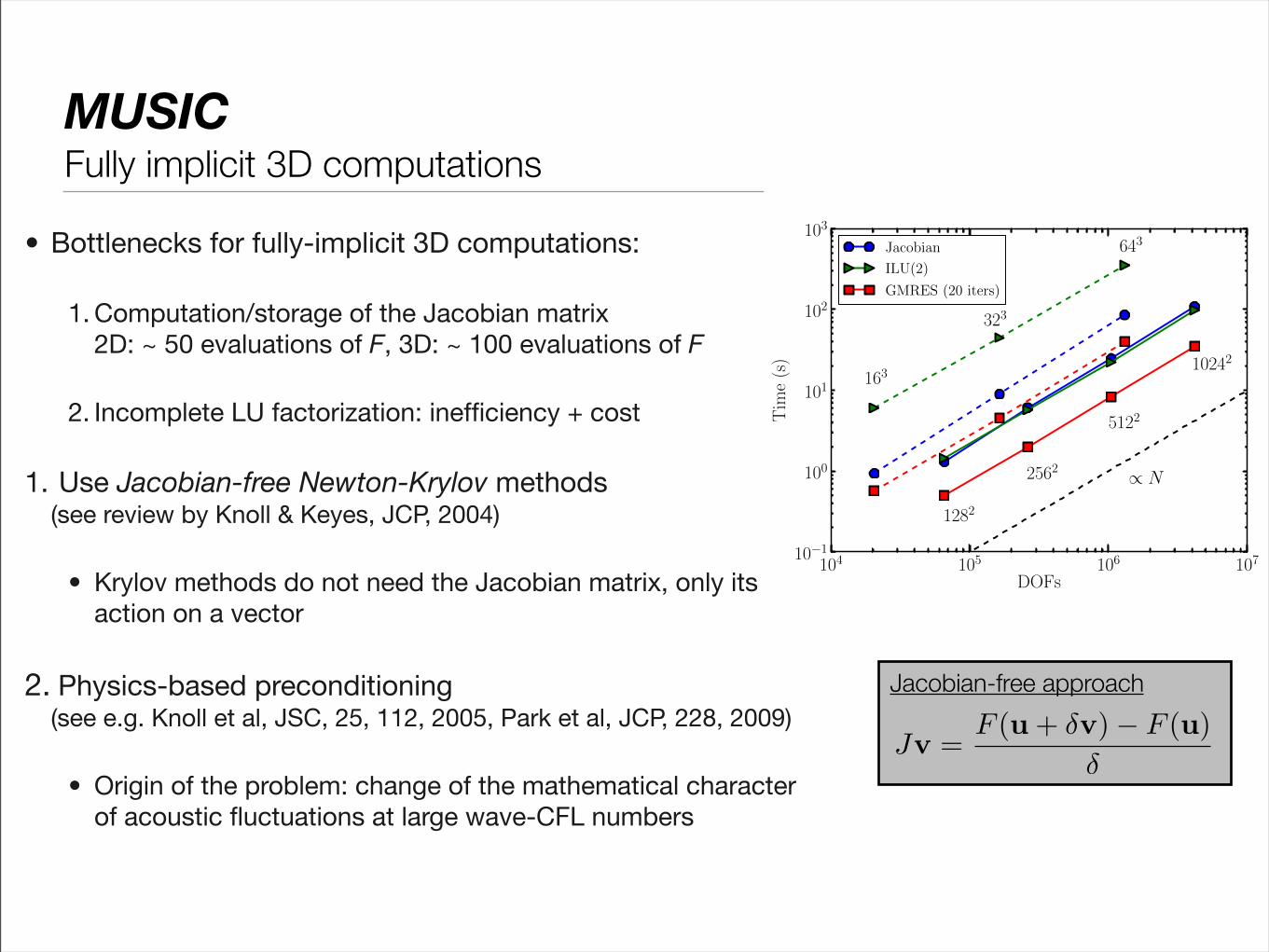
• Bottlenecks for fully-implicit 3D computations:

1. Computation/storage of the Jacobian matrix2D: ~ 50 evaluations of F, 3D: ~ 100 evaluations of F

2. Incomplete LU factorization: inefficiency + cost

1. Use Jacobian-free Newton-Krylov methods(see review by Knoll & Keyes, JCP, 2004)

• Krylov methods do not need the Jacobian matrix, only its action on a vector

2. Physics-based preconditioning(see e.g. Knoll et al, JSC, 25, 112, 2005, Park et al, JCP, 228, 2009)

• Origin of the problem: change of the mathematical character of acoustic fluctuations at large wave-CFL numbers

MUSICFully implicit 3D computations

Jv =F (u+ δv)− F (u)

δ

Jacobian-free approach

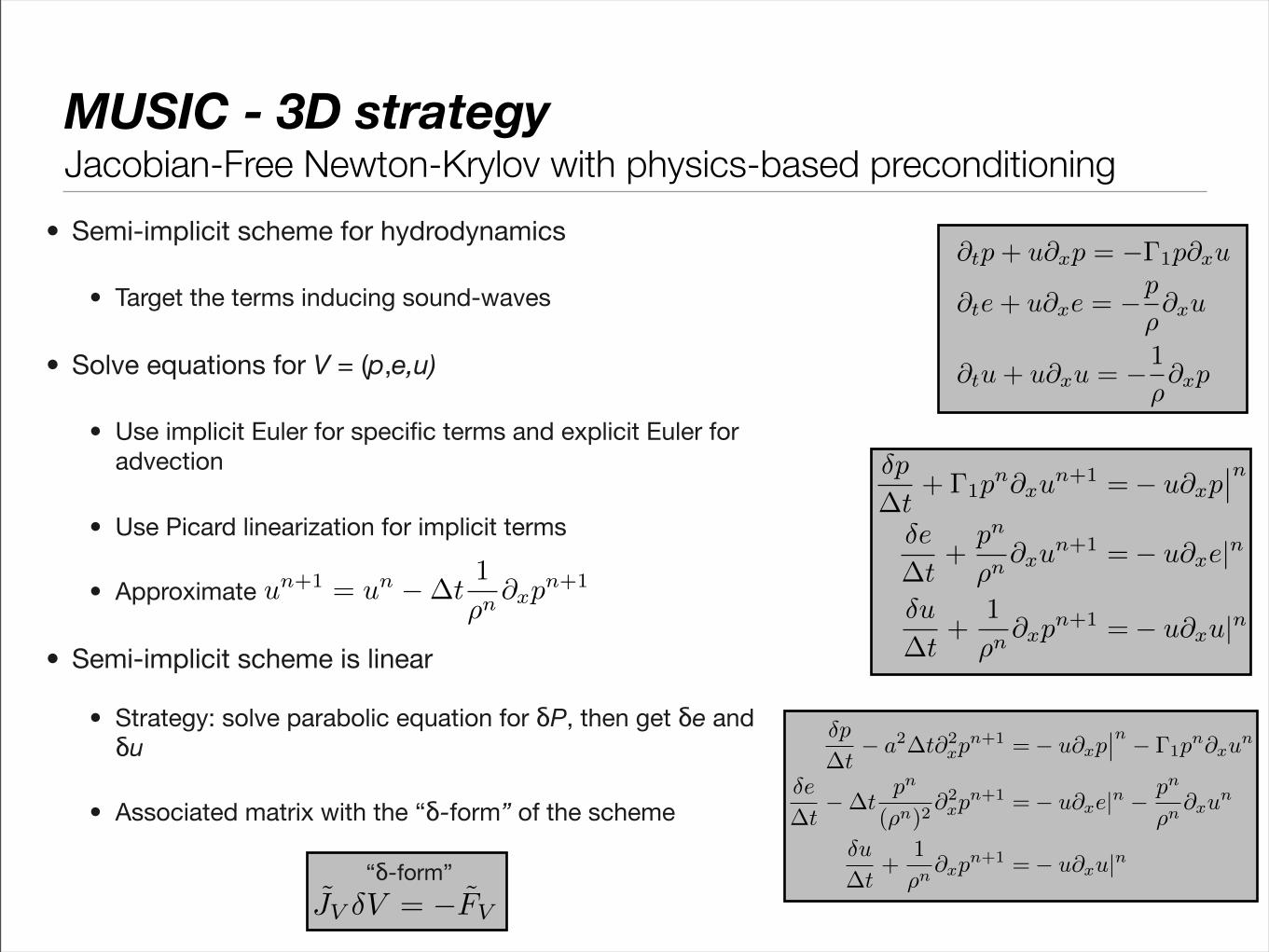
• Semi-implicit scheme for hydrodynamics

• Target the terms inducing sound-waves

• Solve equations for V = (p,e,u)

• Use implicit Euler for specific terms and explicit Euler for advection

• Use Picard linearization for implicit terms

• Approximate

• Semi-implicit scheme is linear

• Strategy: solve parabolic equation for δP, then get δe and δu

• Associated matrix with the “δ-form” of the scheme

MUSIC - 3D strategyJacobian-Free Newton-Krylov with physics-based preconditioning

δp

∆t+ Γ1p

n∂xun+1 =− u∂xp

��n

δe

∆t+

pn

ρn∂xu

n+1 =− u∂xe|n

δu

∆t+

1

ρn∂xp

n+1 =− u∂xu|n

∂tp+ u∂xp = −Γ1p∂xu

∂te+ u∂xe = −p

ρ∂xu

∂tu+ u∂xu = −1

ρ∂xp

δp

∆t− a2∆t∂2

xpn+1 =− u∂xp

��n − Γ1pn∂xu

n

δe

∆t−∆t

pn

(ρn)2∂2xp

n+1 =− u∂xe|n − pn

ρn∂xu

n

δu

∆t+

1

ρn∂xp

n+1 =− u∂xu|n

J̃V δV = −F̃V

“δ-form”

un+1 = un −∆t1

ρn∂xp

n+1

• Test of the semi-implicit scheme

• Advection of an isotropic vortex in 2D

• Scheme is not prone to a wave-CFL condition

• But advection limits the time step (CFLadv ≲ 0.2)

MUSIC - 3D strategyJacobian-Free Newton-Krylov with physics-based preconditioning

10−2 10−1 100 101CFLadv

10−6

10−5

10−4

10−3

10−2

10−1

Normsof

theerror

∝ ∆t

T∞ = 1010

L1-norm

L2-norm

L∞-norm

103 104 105 106CFLhydro

10−2 10−1 100 101CFLadv

10−6

10−5

10−4

10−3

10−2

10−1

Normsof

theerror

∝ ∆t

T∞ = 1

L1-norm

L2-norm

L∞-norm

10−1 100 101CFLhydro

Ms = 0.1 Ms = 10−6

CFLhydro = max� |u|+ cs

∆x

�∆t

CFLadv = max� |u|∆x

�∆t

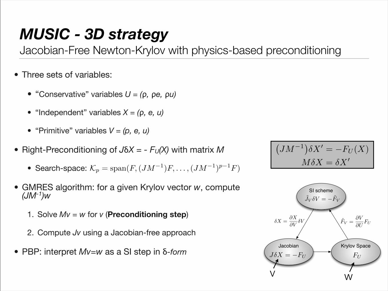
• Three sets of variables:

• “Conservative” variables U = (ρ, ρe, ρu)

• “Independent” variables X = (ρ, e, u)

• “Primitive” variables V = (p, e, u)

• Right-Preconditioning of JδX = - FU(X) with matrix M

• Search-space:

• GMRES algorithm: for a given Krylov vector w, compute(JM-1)w

1. Solve Mv = w for v (Preconditioning step)

2. Compute Jv using a Jacobian-free approach

• PBP: interpret Mv=w as a SI step in δ-form

MUSIC - 3D strategyJacobian-Free Newton-Krylov with physics-based preconditioning

�JM−1

�δX � = −FU (X)

MδX = δX �

SI schemeJ̃V δV = −F̃V

F̃V =∂V

∂UFUδX =

∂X

∂VδV

Jacobian

JδX = −FU

Krylov Space

FU

Kp = span(F, (JM−1)F, . . . , (JM−1)p−1F )

wv

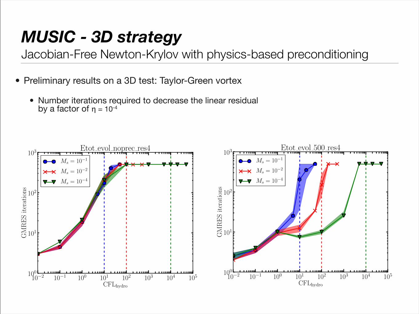
• Preliminary results on a 3D test: Taylor-Green vortex

• Number iterations required to decrease the linear residual by a factor of η = 10-4

MUSIC - 3D strategyJacobian-Free Newton-Krylov with physics-based preconditioning

10−2 10−1 100 101 102 103 104 105CFLhydro

100

101

102

103

GMRESiterations

Etot evol noprec res4

Ms = 10−1

Ms = 10−2

Ms = 10−4

10−2 10−1 100 101 102 103 104 105CFLhydro

100

101

102

103

GMRESiterations

Etot evol 500 res4

Ms = 10−1

Ms = 10−2

Ms = 10−4

Outline

• Introduction

• Newton-Krylov solvers

• Conclusion

• Jacobian-Free Newton-Krylov method for hydrodynamics

• Stiffness spoils the convergence of the Krylov solver

• The preconditioner is the most important ingredient !

• If you know any linear method that yields an approximate solution of your (nonlinear) problem, embedding it within a JFNK method will give you the accuracy

• Unlike algebraic preconditioning, physics-based preconditioning cures the stiffness at the level of the physical model

• Pro: obtain maximum efficiency

• Contra: problem dependent

• Free lunch: semi-implicit schemes also provide a better initial guess for NR

• Additional physics can be included in the preconditioner

• Thermal diffusion: results in two coupled parabolic equations for p and e

Conclusion

END