(Typed) λ-Calculus and Formalising Mathematics `a la de Bruijn In … · 2010-10-07 · let...

(Typed) λ-Calculus and Formalising Mathematics

a la de Bruijn

In honour of De Bruijn’s 90th anniversary

Fairouz Kamareddine (Heriot-Watt University)

5 September 2008

Eindhoven, September 2008

De Bruijn in 1967

• In 1967, an internationally renowned mathematician called N.G. de Bruijnwanted to do something never done before: use the computer to formallycheck the correctness of mathematical books.

• Such a task needs a good formalisation of mathematics, a good competencein implementation, and extreme attention to all the details so that nothing isleft informal.

• No earlier formalisation of mathematics (Frege, Russell, Whitehead, Hilbert,Ramsey, etc.) had ever achieved such attention to details.

• Implementing extensive formal systems on the computer was never done before.

• De Bruijn, an extremely original mathematician, did every step his own way,quickly replacing existing ideas with his own original genious way of thinking,shaping the road ahead for everyone else to follow.

Eindhoven, September 2008 1

De Bruijn in 1967

• When de Bruijn announced his new project Automath at the start of January1967, there was mixed reactions:

– We are talking about respected N.G. de Bruijn who is known to produceideas of gold so the project was bound to gain support.

– The project is so new, so revolutionary, so, it obviously gained opposition:∗ Amongst mathematicians: Why is de Bruijn defecting?∗ Amongst computer scientists: De Bruijn is not a computer scientist so

why is he coming to do a computer scientist’s job?∗ Amongst logicians: De Bruijn is not a logician and has he also forgotten

about Goedel’s undecidability results?

• But, de Bruijn was ahead of everyone else. He is a living genious whose evenscribbled ideas require a life devotion from us ordinary mortal researchers.


• It goes without saying that de Bruijn and his Automath shaped the way.

• It is known that de Bruijn is the father and initiator of Logical frameworks.

• In particular, de Bruijn’s Automath was hugely influential in the developmentof the Edinburgh Logical Frameworks.

• Constable’s Nuprl project has been throughout its development, closelyconnected to ideas in de Bruijn’s Automath (e.g., telescopes).

• Coquand and Huet’s calculus of constructions and consequently the proofchecker Coq were heavily influenced by de Bruijn’s dependent types, PAT andAutomath.

• De Bruijn was the first to put the Propositions As Types (PAT) idea in practice.

• Barendregt’s cube and Pure Type systems are a beautiful example of thegenerality of the typing rules of Automath.


• De Bruijn was the first to express the importance of definitions to theformalisation and proof checking of mathematics. Definitions (also known aslet expressions) have been adopted in other proof checkers and in programminglanguges (e.g. ML).

• De Bruijn’s Automath was the first (and remains the only) proof checker inwhich an entire book has been fully proof checked by the computer (Mizar isthe next system in which 60% of a book is proof checked).

• There are numerous other gems in de Bruijn’s Automath.

• It has been, and will be for many generations to come, a hard but magicaltask to fully decode the genious ideas of de Bruijn in his Automath project.

• In this talk, I will concentrate on some low level details which explain whyevery sentence in de Bruijn’s writing is a gem that can help us solve numerousproblems in current research in programming language theory/implementationand in logical frameworks.


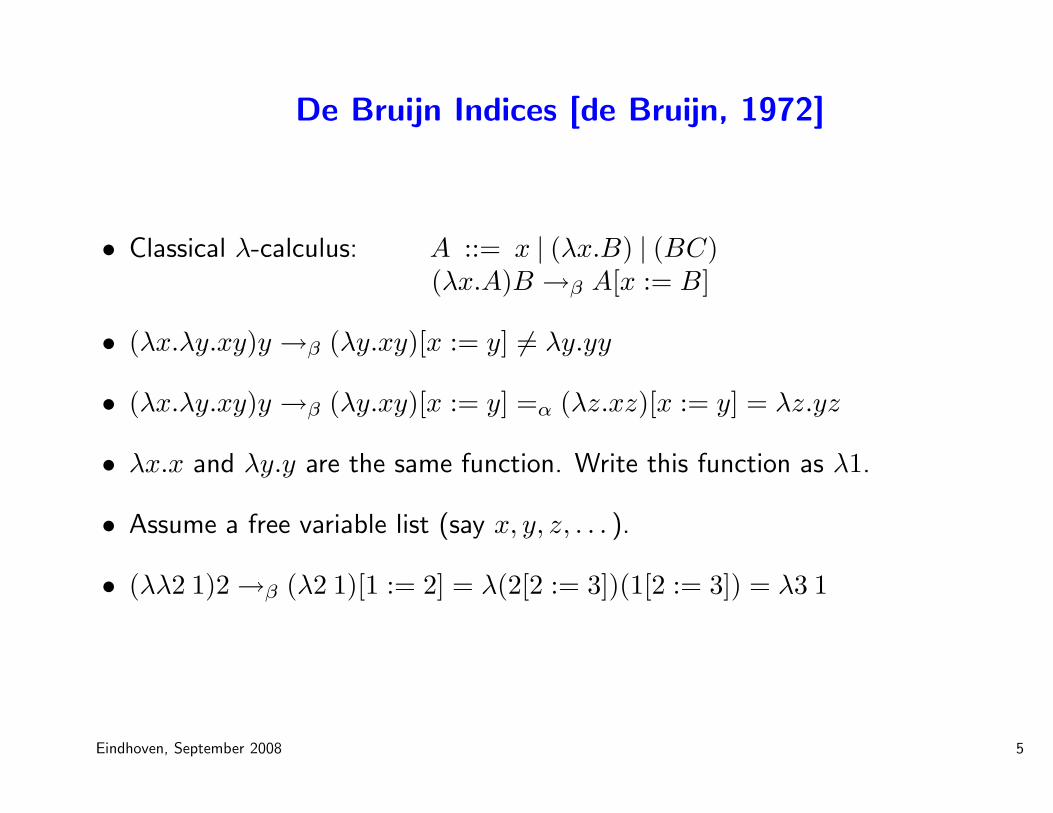
De Bruijn Indices [de Bruijn, 1972]

• Classical λ-calculus: A ::= x | (λx.B) | (BC)(λx.A)B →β A[x := B]

• (λx.λy.xy)y →β (λy.xy)[x := y] 6= λy.yy

• (λx.λy.xy)y →β (λy.xy)[x := y] =α (λz.xz)[x := y] = λz.yz

• λx.x and λy.y are the same function. Write this function as λ1.

• Assume a free variable list (say x, y, z, . . . ).

• (λλ2 1)2→β (λ2 1)[1 := 2] = λ(2[2 := 3])(1[2 := 3]) = λ3 1


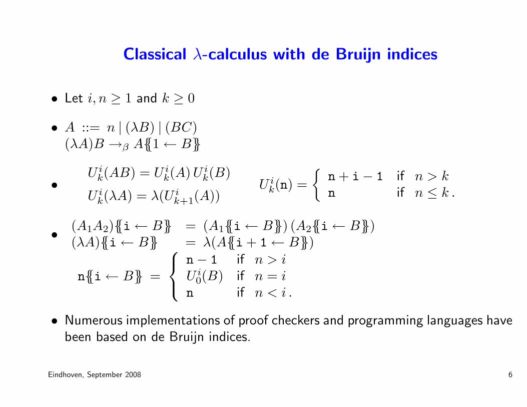
Classical λ-calculus with de Bruijn indices

• Let i, n ≥ 1 and k ≥ 0

• A ::= n | (λB) | (BC)(λA)B →β A{{1← B}}

•U i

k(AB) = U ik(A) U i

k(B)

U ik(λA) = λ(U i

k+1(A))U i

k(n) =

{

n + i− 1 if n > kn if n ≤ k .

•(A1A2){{i← B}} = (A1{{i← B}}) (A2{{i← B}})(λA){{i← B}} = λ(A{{i + 1← B}})

n{{i← B}} =

n− 1 if n > iU i

0(B) if n = in if n < i .

• Numerous implementations of proof checkers and programming languages havebeen based on de Bruijn indices.


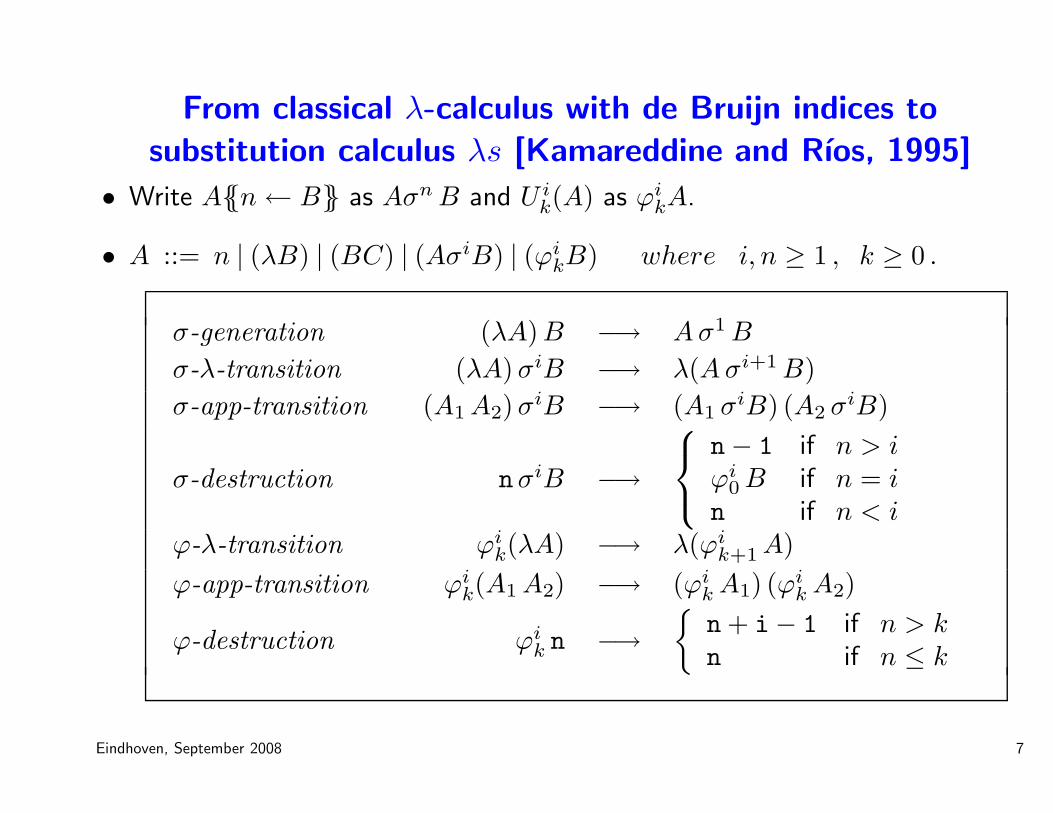
From classical λ-calculus with de Bruijn indices to

substitution calculus λs [Kamareddine and Rıos, 1995]

• Write A{{n← B}} as Aσn B and U ik(A) as ϕi

kA.

• A ::= n | (λB) | (BC) | (AσiB) | (ϕikB) where i, n ≥ 1 , k ≥ 0 .

σ-generation (λA) B −→ A σ1 B

σ-λ-transition (λA) σiB −→ λ(A σi+1 B)

σ-app-transition (A1 A2) σiB −→ (A1 σiB) (A2 σiB)

σ-destruction nσiB −→

n− 1 if n > iϕi

0 B if n = in if n < i

ϕ-λ-transition ϕik(λA) −→ λ(ϕi

k+1 A)

ϕ-app-transition ϕik(A1 A2) −→ (ϕi

k A1) (ϕik A2)

ϕ-destruction ϕik n −→

{

n + i− 1 if n > kn if n ≤ k


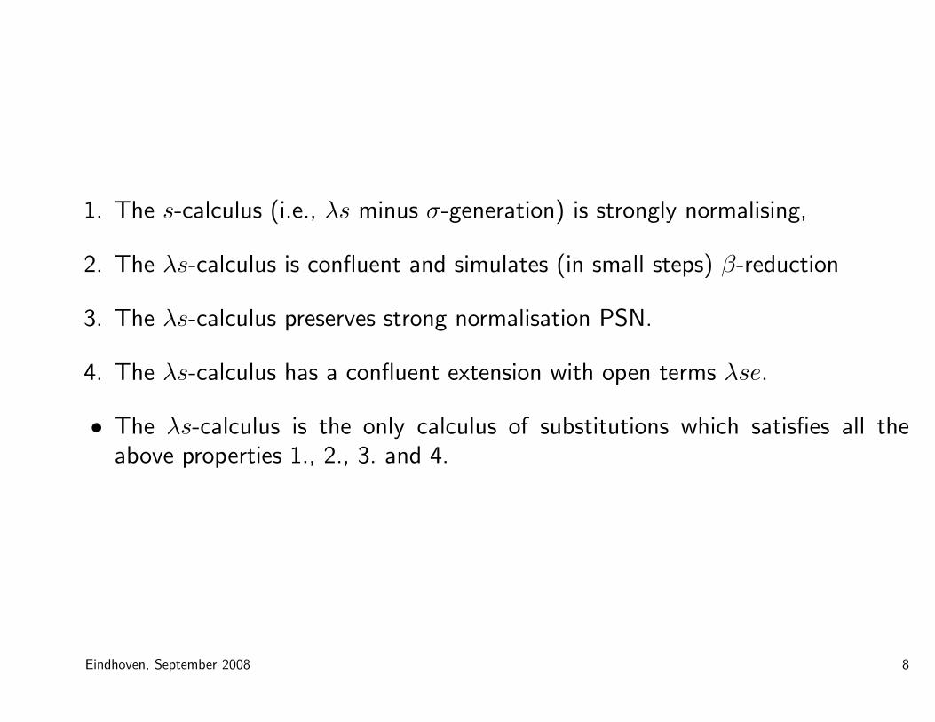
1. The s-calculus (i.e., λs minus σ-generation) is strongly normalising,

2. The λs-calculus is confluent and simulates (in small steps) β-reduction

3. The λs-calculus preserves strong normalisation PSN.

4. The λs-calculus has a confluent extension with open terms λse.

• The λs-calculus is the only calculus of substitutions which satisfies all theabove properties 1., 2., 3. and 4.


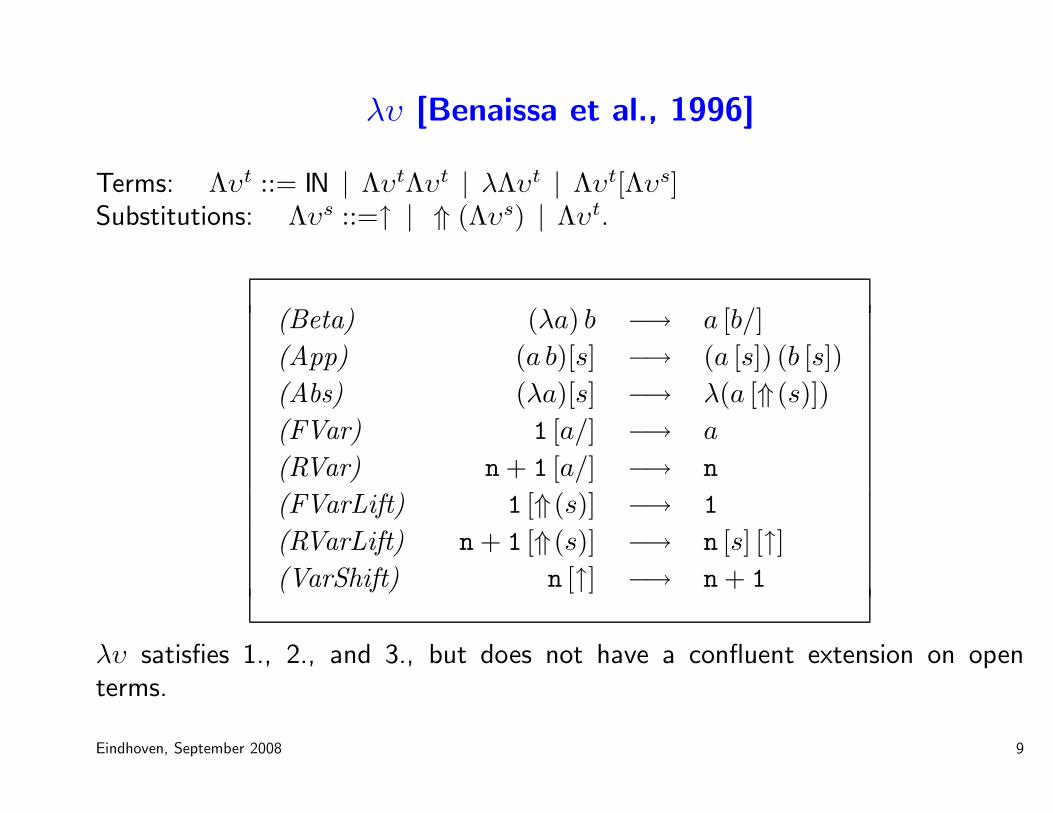
λυ [Benaissa et al., 1996]

Terms: Λυt ::= IN | ΛυtΛυt | λΛυt | Λυt[Λυs]Substitutions: Λυs ::=↑ | ⇑ (Λυs) | Λυt.

(Beta) (λa) b −→ a [b/]

(App) (a b)[s] −→ (a [s]) (b [s])

(Abs) (λa)[s] −→ λ(a [⇑(s)])

(FVar) 1 [a/] −→ a

(RVar) n + 1 [a/] −→ n

(FVarLift) 1 [⇑(s)] −→ 1

(RVarLift) n + 1 [⇑(s)] −→ n [s] [↑]

(VarShift) n [↑] −→ n + 1

λυ satisfies 1., 2., and 3., but does not have a confluent extension on openterms.


λσ⇑

Terms: Λσt⇑ ::= IN | Λσt

⇑Λσt⇑ | λΛσt

⇑ | Λσt⇑[Λσs

⇑]Substitutions: Λσs

⇑ ::= id | ↑ | ⇑ (Λσs⇑) | Λσt

⇑ · Λσs⇑ | Λσs

⇑ ◦ Λσs⇑.

(Beta) (λa) b −→ a [b · id]

(App) (a b)[s] −→ (a [s]) (b [s])

(Abs) (λa)[s] −→ λ(a [⇑(s)])

(Clos) (a [s])[t] −→ a [s ◦ t]

(Varshift1) n [↑] −→ n + 1

(Varshift2) n [↑ ◦ s] −→ n + 1 [s]

(FVarCons) 1 [a · s] −→ a

(RVarCons) n + 1 [a · s] −→ n [s]

(FVarLift1) 1 [⇑(s)] −→ 1

(FVarLift2) 1 [⇑(s) ◦ t] −→ 1 [t]

(RVarLift1) n + 1 [⇑(s)] −→ n[s ◦ ↑]

(RVarLift2) n + 1 [⇑(s) ◦ t] −→ n[s ◦ (↑ ◦ t)]


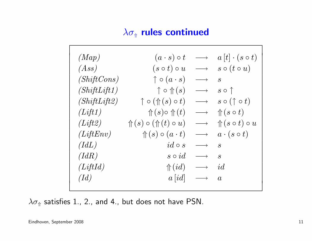
λσ⇑ rules continued

(Map) (a · s) ◦ t −→ a [t] · (s ◦ t)

(Ass) (s ◦ t) ◦ u −→ s ◦ (t ◦ u)

(ShiftCons) ↑ ◦ (a · s) −→ s

(ShiftLift1) ↑ ◦ ⇑(s) −→ s ◦ ↑

(ShiftLift2) ↑ ◦ (⇑(s) ◦ t) −→ s ◦ (↑ ◦ t)

(Lift1) ⇑(s)◦ ⇑(t) −→ ⇑(s ◦ t)

(Lift2) ⇑(s) ◦ (⇑(t) ◦ u) −→ ⇑(s ◦ t) ◦ u

(LiftEnv) ⇑(s) ◦ (a · t) −→ a · (s ◦ t)

(IdL) id ◦ s −→ s

(IdR) s ◦ id −→ s

(LiftId) ⇑(id) −→ id

(Id) a [id] −→ a

λσ⇑ satisfies 1., 2., and 4., but does not have PSN.


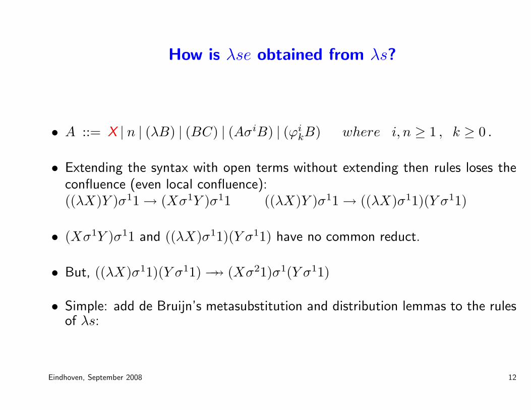
How is λse obtained from λs?

• A ::= X | n | (λB) | (BC) | (AσiB) | (ϕikB) where i, n ≥ 1 , k ≥ 0 .

• Extending the syntax with open terms without extending then rules loses theconfluence (even local confluence):((λX)Y )σ11→ (Xσ1Y )σ11 ((λX)Y )σ11→ ((λX)σ11)(Y σ11)

• (Xσ1Y )σ11 and ((λX)σ11)(Y σ11) have no common reduct.

• But, ((λX)σ11)(Y σ11)→→ (Xσ21)σ1(Y σ11)

• Simple: add de Bruijn’s metasubstitution and distribution lemmas to the rulesof λs:


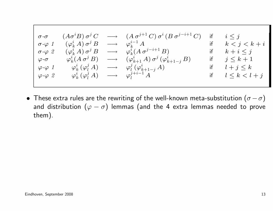
σ-σ (AσiB) σj C −→ (A σj+1 C) σi (B σj−i+1 C) if i ≤ j

σ-ϕ 1 (ϕik A) σj B −→ ϕi−1

k A if k < j < k + i

σ-ϕ 2 (ϕik A) σj B −→ ϕi

k(A σj−i+1 B) if k + i ≤ j

ϕ-σ ϕik(A σj B) −→ (ϕi

k+1 A) σj (ϕik+1−j B) if j ≤ k + 1

ϕ-ϕ 1 ϕik (ϕj

l A) −→ ϕjl (ϕi

k+1−j A) if l + j ≤ k

ϕ-ϕ 2 ϕik (ϕj

l A) −→ ϕj+i−1l A if l ≤ k < l + j

• These extra rules are the rewriting of the well-known meta-substitution (σ−σ)and distribution (ϕ − σ) lemmas (and the 4 extra lemmas needed to provethem).


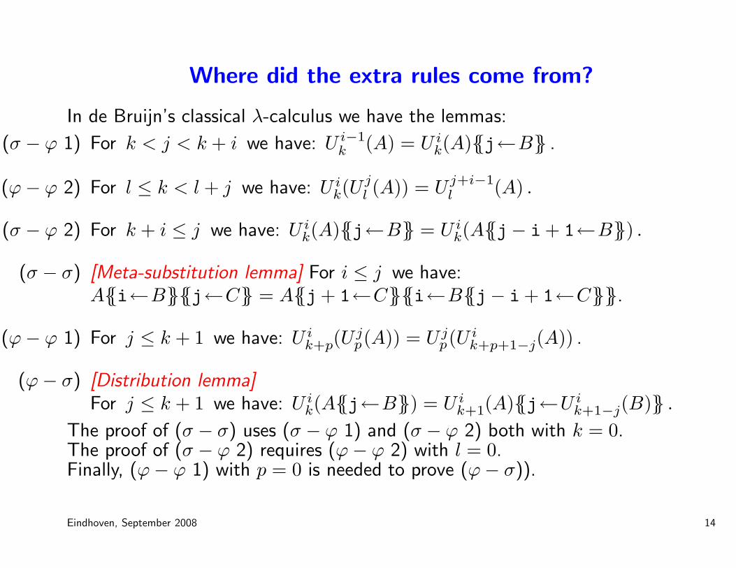
Where did the extra rules come from?

In de Bruijn’s classical λ-calculus we have the lemmas:

(σ − ϕ 1) For k < j < k + i we have: U i−1k (A) = U i

k(A){{j←B}} .

(ϕ− ϕ 2) For l ≤ k < l + j we have: U ik(U

jl (A)) = U j+i−1

l (A) .

(σ − ϕ 2) For k + i ≤ j we have: U ik(A){{j←B}} = U i

k(A{{j− i + 1←B}}) .

(σ − σ) [Meta-substitution lemma] For i ≤ j we have:A{{i←B}}{{j←C}} = A{{j + 1←C}}{{i←B{{j− i + 1←C}}}}.

(ϕ− ϕ 1) For j ≤ k + 1 we have: U ik+p(U

jp(A)) = U j

p(U ik+p+1−j(A)) .

(ϕ− σ) [Distribution lemma]For j ≤ k + 1 we have: U i

k(A{{j←B}}) = U ik+1(A){{j←U i

k+1−j(B)}} .

The proof of (σ − σ) uses (σ − ϕ 1) and (σ − ϕ 2) both with k = 0.The proof of (σ − ϕ 2) requires (ϕ− ϕ 2) with l = 0.Finally, (ϕ− ϕ 1) with p = 0 is needed to prove (ϕ− σ)).


Summary of [de Bruijn, 1972]

• Those who in 1967 said that de Bruijn was not a computer scientist, musthave felt embarassed afterwards.

• De Bruijn’s work not only had serious consequences on the implementationof numerous programming languages and proof checkers, but also was todominate decades of research and hundreds of articles by many researchers.

• Here, I described how his work in [de Bruijn, 1972] influenced research intocalculi of explicit substitutions.

• Next I describe how his novel notation for the λ-calculus influenced notions ofgeneralised reductions (with implications on theoretical and implementationalaspects of the λ-calculus and programming languages).


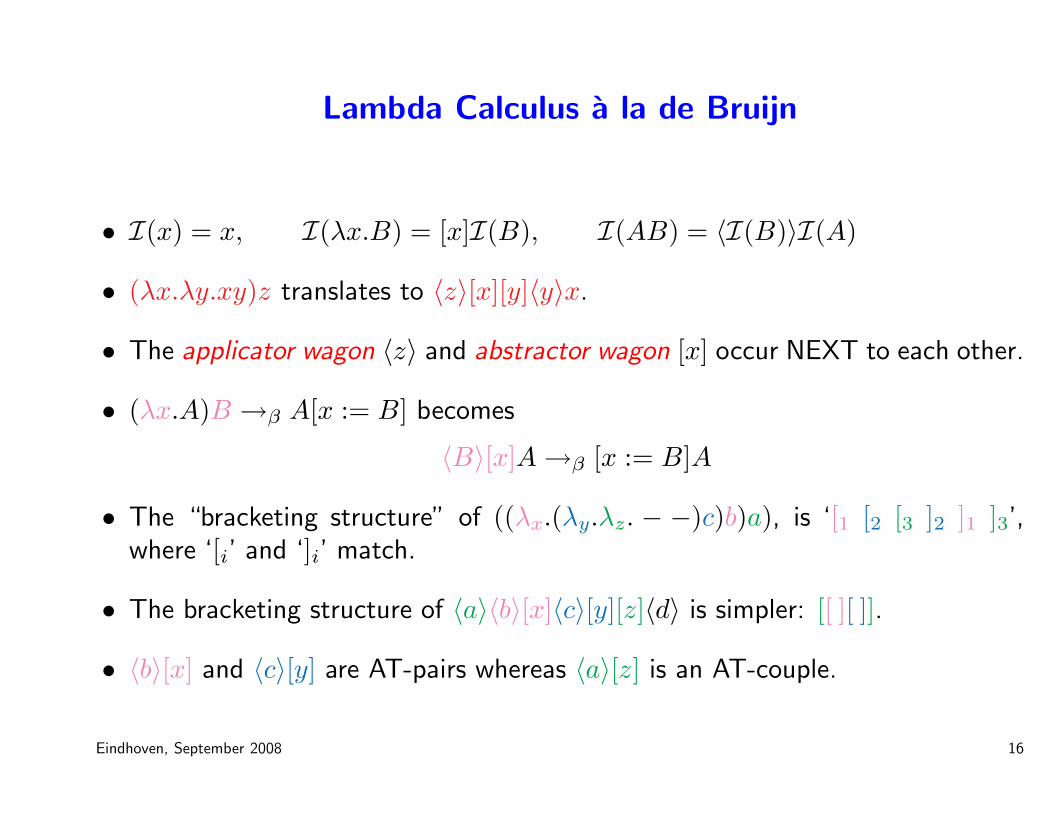
Lambda Calculus a la de Bruijn

• I(x) = x, I(λx.B) = [x]I(B), I(AB) = 〈I(B)〉I(A)

• (λx.λy.xy)z translates to 〈z〉[x][y]〈y〉x.

• The applicator wagon 〈z〉 and abstractor wagon [x] occur NEXT to each other.

• (λx.A)B →β A[x := B] becomes

〈B〉[x]A→β [x := B]A

• The “bracketing structure” of ((λx.(λy.λz. − −)c)b)a), is ‘[1 [2 [3 ]2 ]1 ]3’,where ‘[i’ and ‘]i’ match.

• The bracketing structure of 〈a〉〈b〉[x]〈c〉[y][z]〈d〉 is simpler: [[ ][ ]].

• 〈b〉[x] and 〈c〉[y] are AT-pairs whereas 〈a〉[z] is an AT-couple.


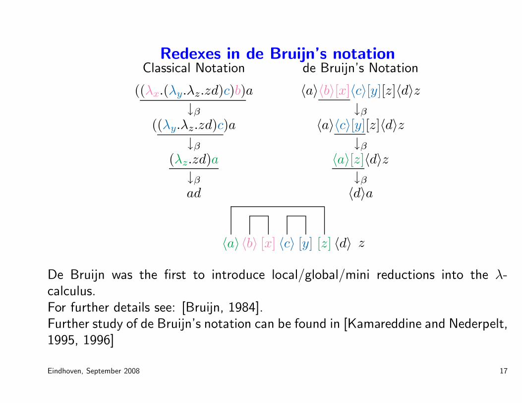
Redexes in de Bruijn’s notationClassical Notation de Bruijn’s Notation

((λx.(λy.λz.zd)c)b)a 〈a〉〈b〉[x]〈c〉[y][z]〈d〉z

↓β ↓β((λy.λz.zd)c)a 〈a〉〈c〉[y][z]〈d〉z

↓β ↓β(λz.zd)a 〈a〉[z]〈d〉z

↓β ↓βad 〈d〉a

〈a〉〈b〉 [x] 〈c〉 [y] [z] 〈d〉 z

De Bruijn was the first to introduce local/global/mini reductions into the λ-calculus.For further details see: [Bruijn, 1984].Further study of de Bruijn’s notation can be found in [Kamareddine and Nederpelt,1995, 1996]


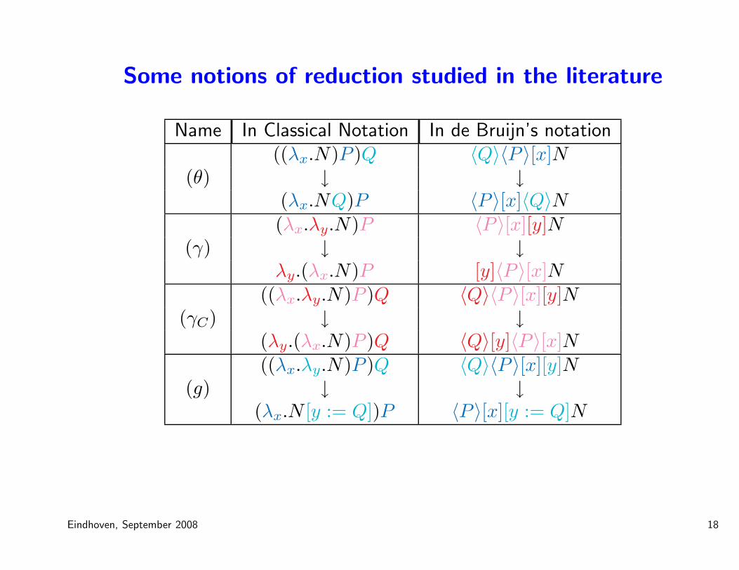
Some notions of reduction studied in the literature

Name In Classical Notation In de Bruijn’s notation((λx.N)P )Q 〈Q〉〈P 〉[x]N

(θ) ↓ ↓(λx.NQ)P 〈P 〉[x]〈Q〉N(λx.λy.N)P 〈P 〉[x][y]N

(γ) ↓ ↓λy.(λx.N)P [y]〈P 〉[x]N

((λx.λy.N)P )Q 〈Q〉〈P 〉[x][y]N(γC) ↓ ↓

(λy.(λx.N)P )Q 〈Q〉[y]〈P 〉[x]N((λx.λy.N)P )Q 〈Q〉〈P 〉[x][y]N

(g) ↓ ↓(λx.N [y := Q])P 〈P 〉[x][y := Q]N


A Few Uses of these reductions/term reshuffling

• Regnier [1992] uses θ and γ in analyzing perpetual reduction strategies.

• Term reshuffling is used in [Kfoury et al., 1994; Kfoury and Wells, 1994] inanalyzing typability problems.

• [Nederpelt, 1973; de Groote, 1993; Kfoury and Wells, 1995] use generalisedreduction and/or term reshuffling in relating SN to WN.

• [Ariola et al., 1995] uses a form of term-reshuffling in obtaining a calculus thatcorresponds to lazy functional evaluation.

• [Kamareddine and Nederpelt, 1995; Kamareddine et al., 1999, 1998; Blooet al., 1996] shows that they could reduce space/time needs.

• [Kamareddine, 2000] shows the conservation theorem for generalised reduction.

• All these works have been heavily influenced by de Bruijn’s Automath whoseλ-notation facilitated the manipulation of redexes.


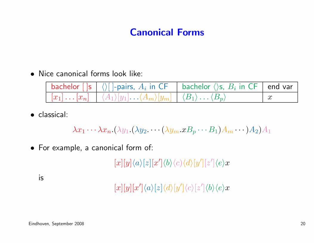
Canonical Forms

• Nice canonical forms look like:

bachelor [ ]s 〈〉[ ]-pairs, Ai in CF bachelor 〈〉s, Bi in CF end var[x1] . . . [xn] 〈A1〉[y1]. . .〈Am〉[ym] 〈B1〉 . . . 〈Bp〉 x

• classical:

λx1 · · ·λxn.(λy1.(λy2. · · · (λym.xBp · · ·B1)Am · · · )A2)A1

• For example, a canonical form of:

[x][y]〈a〉[z][x′]〈b〉〈c)〈d〉[y′][z′]〈e〉x

is[x][y][x′]〈a〉[z]〈d〉[y′]〈c〉[z′]〈b〉〈e〉x


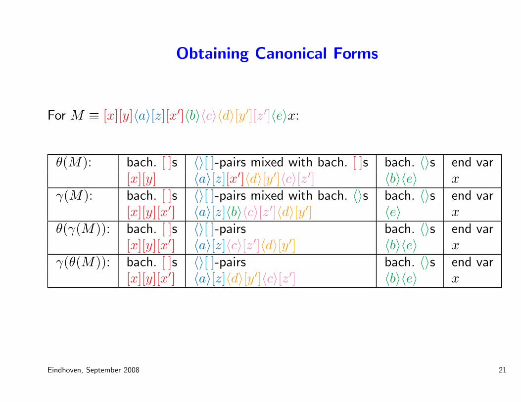
Obtaining Canonical Forms

For M ≡ [x][y]〈a〉[z][x′]〈b〉〈c〉〈d〉[y′][z′]〈e〉x:

θ(M): bach. [ ]s 〈〉[ ]-pairs mixed with bach. [ ]s bach. 〈〉s end var[x][y] 〈a〉[z][x′]〈d〉[y′]〈c〉[z′] 〈b〉〈e〉 x

γ(M): bach. [ ]s 〈〉[ ]-pairs mixed with bach. 〈〉s bach. 〈〉s end var[x][y][x′] 〈a〉[z]〈b〉〈c〉[z′]〈d〉[y′] 〈e〉 x

θ(γ(M)): bach. [ ]s 〈〉[ ]-pairs bach. 〈〉s end var[x][y][x′] 〈a〉[z]〈c〉[z′]〈d〉[y′] 〈b〉〈e〉 x

γ(θ(M)): bach. [ ]s 〈〉[ ]-pairs bach. 〈〉s end var[x][y][x′] 〈a〉[z]〈d〉[y′]〈c〉[z′] 〈b〉〈e〉 x


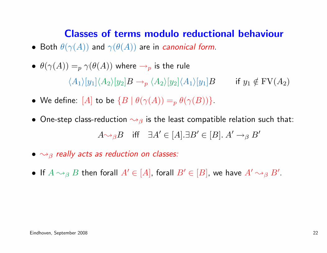
Classes of terms modulo reductional behaviour• Both θ(γ(A)) and γ(θ(A)) are in canonical form.

• θ(γ(A)) =p γ(θ(A)) where →p is the rule

〈A1〉[y1]〈A2〉[y2]B →p 〈A2〉[y2]〈A1〉[y1]B if y1 /∈ FV(A2)

• We define: [A] to be {B | θ(γ(A)) =p θ(γ(B))}.

• One-step class-reduction ;β is the least compatible relation such that:

A;βB iff ∃A′ ∈ [A].∃B′ ∈ [B]. A′ →β B′

• ;β really acts as reduction on classes:

• If A ;β B then forall A′ ∈ [A], forall B′ ∈ [B], we have A′;β B′.


Properties of reduction modulo classes

• ;β generalises →g and →β: →β ⊂→g⊂;β ⊂=β.

• ≈β and =β are equivalent: A ≈β B iff A =β B.

• ;;β is Church Rosser:If A ;;β B and A ;;β C, then for some D: B ;;β D and C ;;β D.

• Classes preserve SN→β: If A ∈ SN→β

and A′ ∈ [A] then A′ ∈ SN→β.

• Classes preserve SN;β: If A ∈ SN;β

and A′ ∈ [A] then A′ ∈ SN;β.

• SN→βand SN;β

are equivalent: A ∈ SN;βiff A ∈ SN→β

.


Typed λ-calculus with single binder

• Let f : N→ N et gf : N→ N such that gf(x) = f(f(x)).

Let FN : (N→ N)→ (N→ N) such that FN(f)(x) = gf(x) = f(f(x)).

• In Church’s simply typed lambda calculus we write the function FN as follows:

λf :N→N.λx:N.f(f(x))

• If we want the same function on the booleans B, we write:

the function FB is λf :B→B.λx:B.f(f(x))the type of the function FB is (B → B)→ (B → B)


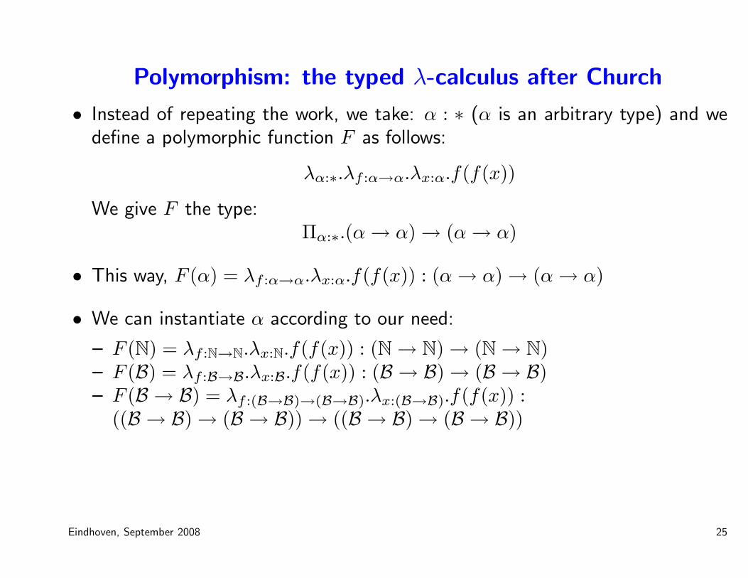
Polymorphism: the typed λ-calculus after Church

• Instead of repeating the work, we take: α : ∗ (α is an arbitrary type) and wedefine a polymorphic function F as follows:

λα:∗.λf :α→α.λx:α.f(f(x))

We give F the type:Πα:∗.(α→ α)→ (α→ α)

• This way, F (α) = λf :α→α.λx:α.f(f(x)) : (α→ α)→ (α→ α)

• We can instantiate α according to our need:

– F (N) = λf :N→N.λx:N.f(f(x)) : (N→ N)→ (N→ N)– F (B) = λf :B→B.λx:B.f(f(x)) : (B → B)→ (B → B)– F (B → B) = λf :(B→B)→(B→B).λx:(B→B).f(f(x)) :

((B → B)→ (B → B))→ ((B → B)→ (B → B))


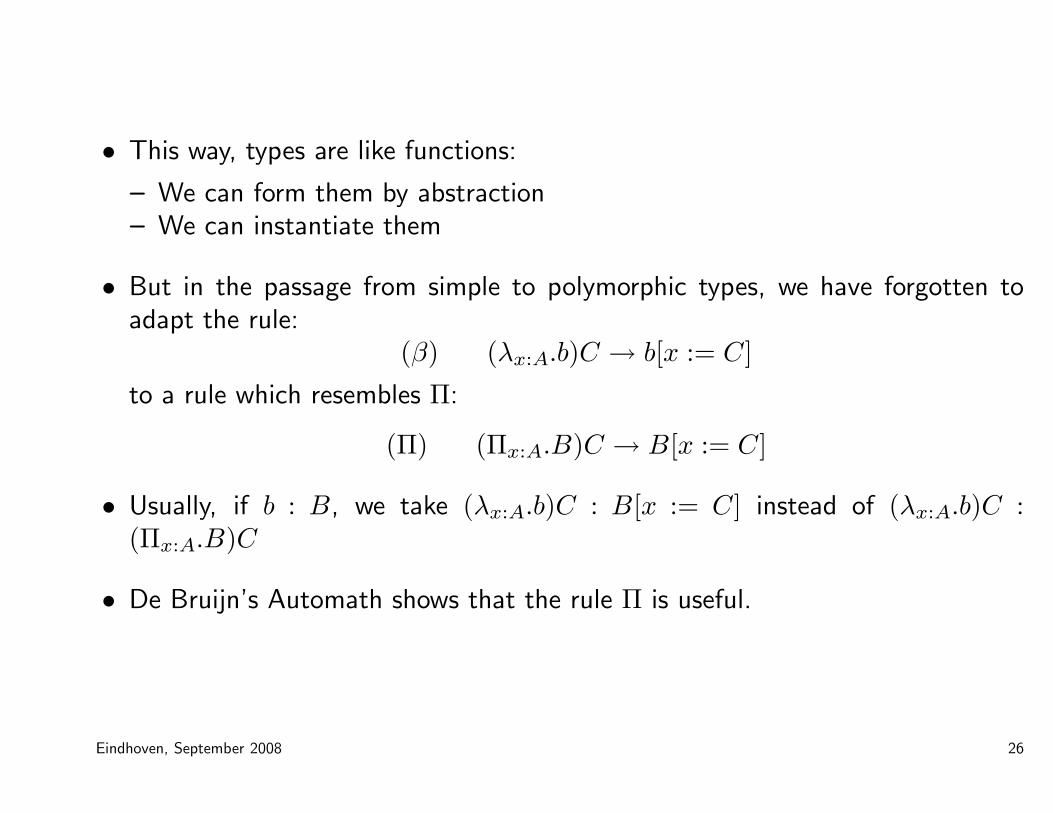
• This way, types are like functions:

– We can form them by abstraction– We can instantiate them

• But in the passage from simple to polymorphic types, we have forgotten toadapt the rule:

(β) (λx:A.b)C → b[x := C]

to a rule which resembles Π:

(Π) (Πx:A.B)C → B[x := C]

• Usually, if b : B, we take (λx:A.b)C : B[x := C] instead of (λx:A.b)C :(Πx:A.B)C

• De Bruijn’s Automath shows that the rule Π is useful.


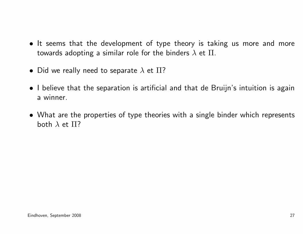
• It seems that the development of type theory is taking us more and moretowards adopting a similar role for the binders λ et Π.

• Did we really need to separate λ et Π?

• I believe that the separation is artificial and that de Bruijn’s intuition is againa winner.

• What are the properties of type theories with a single binder which representsboth λ et Π?


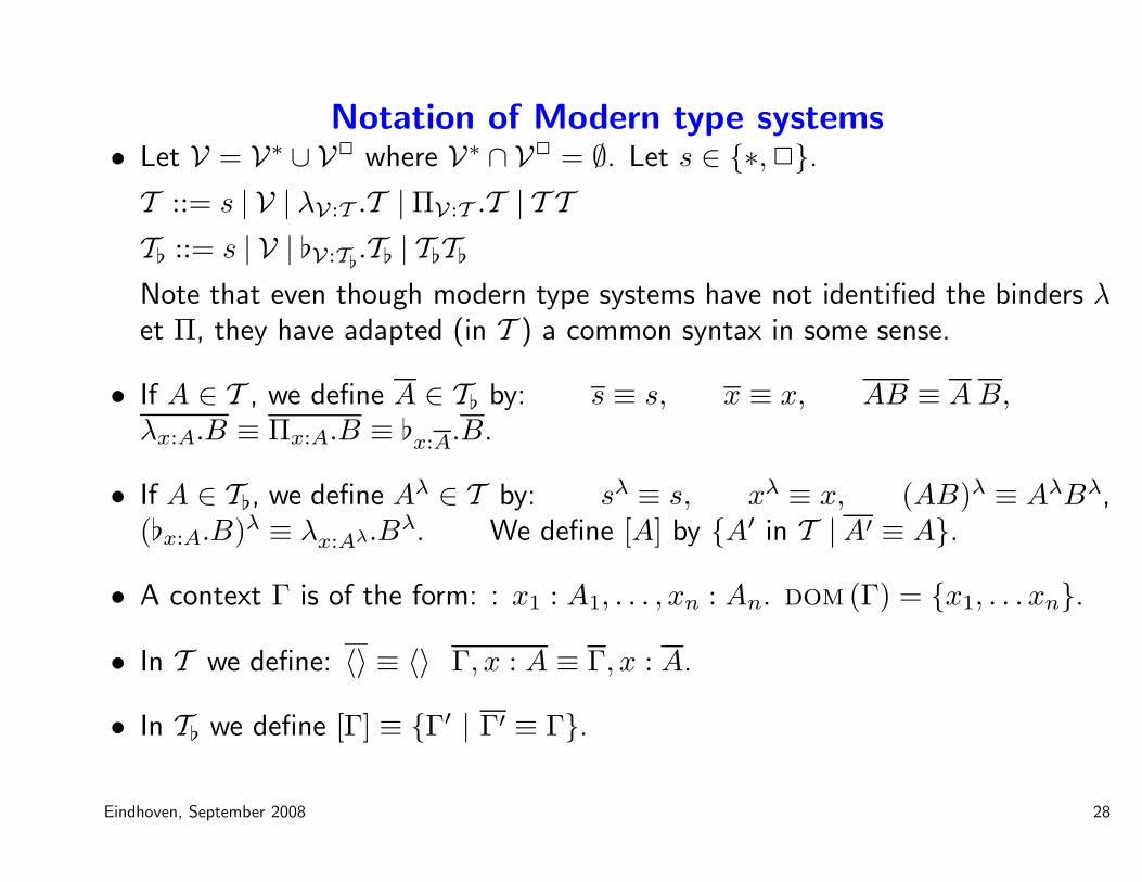
Notation of Modern type systems• Let V = V∗ ∪ V2 where V∗ ∩ V2 = ∅. Let s ∈ {∗, 2}.

T ::= s | V | λV:T .T |ΠV:T .T | T T

T♭ ::= s | V | ♭V:T♭.T♭ | T♭T♭

Note that even though modern type systems have not identified the binders λet Π, they have adapted (in T ) a common syntax in some sense.

• If A ∈ T , we define A ∈ T♭ by: s ≡ s, x ≡ x, AB ≡ A B,λx:A.B ≡ Πx:A.B ≡ ♭x:A.B.

• If A ∈ T♭, we define Aλ ∈ T by: sλ ≡ s, xλ ≡ x, (AB)λ ≡ AλBλ,(♭x:A.B)λ ≡ λx:Aλ.Bλ. We define [A] by {A′ in T |A′ ≡ A}.

• A context Γ is of the form: : x1 : A1, . . . , xn : An. dom (Γ) = {x1, . . . xn}.

• In T we define: 〈〉 ≡ 〈〉 Γ, x : A ≡ Γ, x : A.

• In T♭ we define [Γ] ≡ {Γ′ | Γ′ ≡ Γ}.


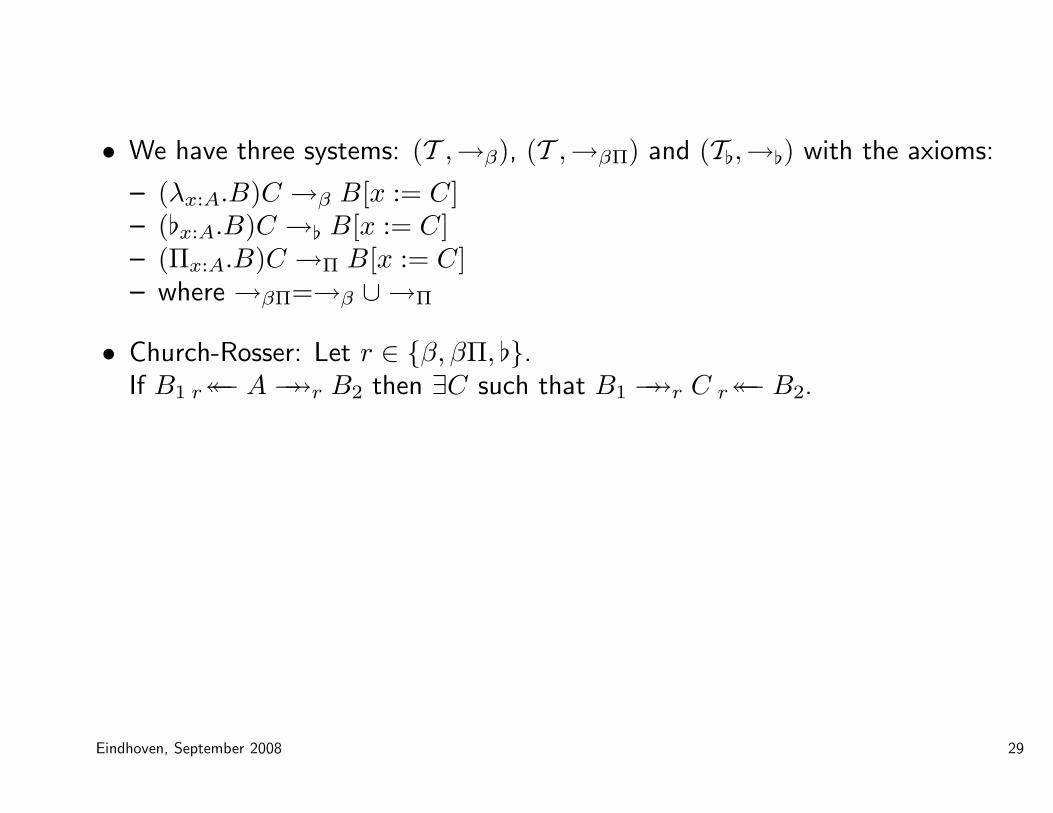
• We have three systems: (T ,→β), (T ,→βΠ) and (T♭,→♭) with the axioms:

– (λx:A.B)C →β B[x := C]– (♭x:A.B)C →♭ B[x := C]– (Πx:A.B)C →Π B[x := C]– where →βΠ=→β ∪ →Π

• Church-Rosser: Let r ∈ {β, βΠ, ♭}.If B1 r←← A→→r B2 then ∃C such that B1→→r C r←← B2.


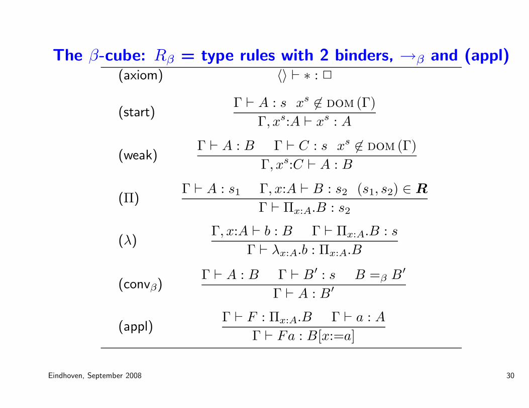
The β-cube: Rβ = type rules with 2 binders, →β and (appl)(axiom) 〈〉 ⊢ ∗ : 2

(start)Γ ⊢ A : s xs 6∈ dom (Γ)

Γ, xs:A ⊢ xs : A

(weak)Γ ⊢ A : B Γ ⊢ C : s xs 6∈ dom (Γ)

Γ, xs:C ⊢ A : B

(Π)Γ ⊢ A : s1 Γ, x:A ⊢ B : s2 (s1, s2) ∈ R

Γ ⊢ Πx:A.B : s2

(λ)Γ, x:A ⊢ b : B Γ ⊢ Πx:A.B : s

Γ ⊢ λx:A.b : Πx:A.B

(convβ)Γ ⊢ A : B Γ ⊢ B′ : s B =β B′

Γ ⊢ A : B′

(appl)Γ ⊢ F : Πx:A.B Γ ⊢ a : A

Γ ⊢ Fa : B[x:=a]


��

��

��

��

�

��

��

��

��

�

��

��

��

��

�

��

��

��

��

�

β→ βP

β2 βP2

βωβPω

βCβω

r r

rr

r r

rr

-

6

��1

(∗, 2) ∈ R

(2,2) ∈ R

(2, ∗) ∈ R

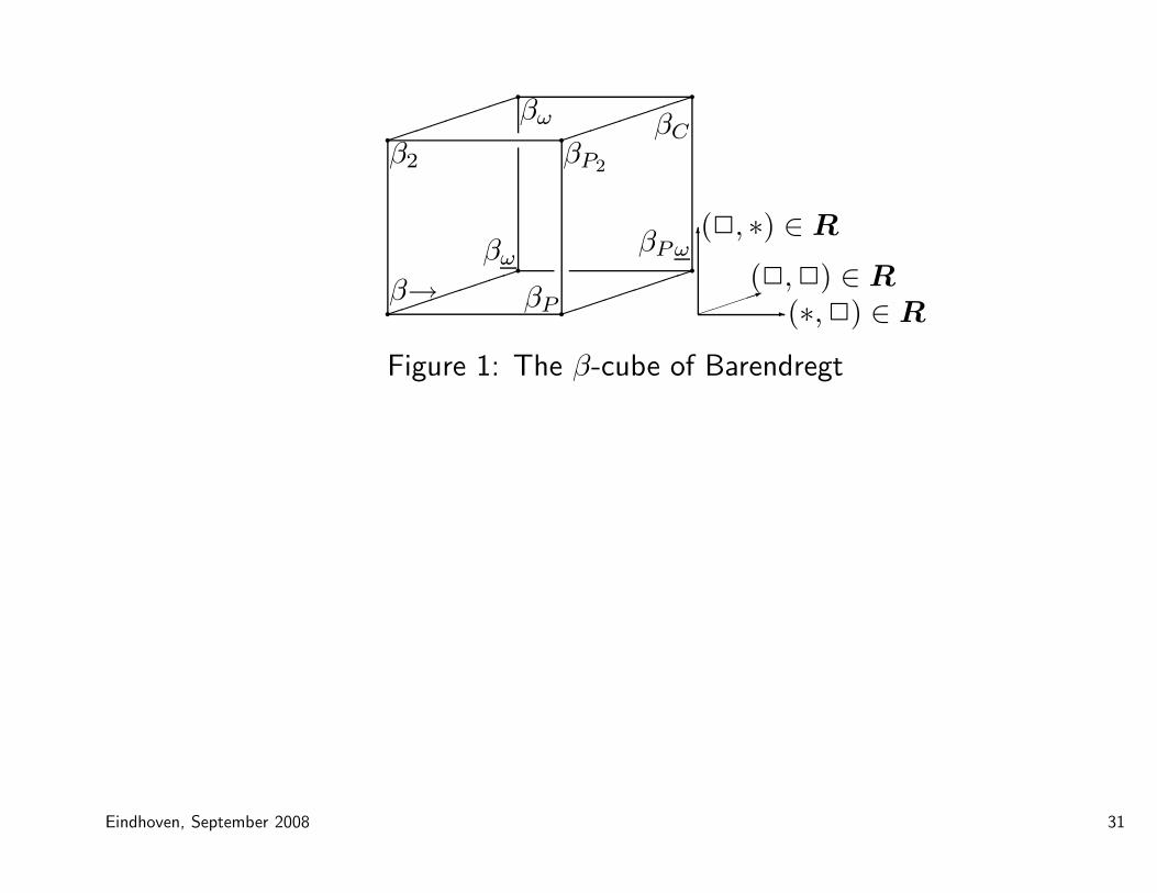
Figure 1: The β-cube of Barendregt


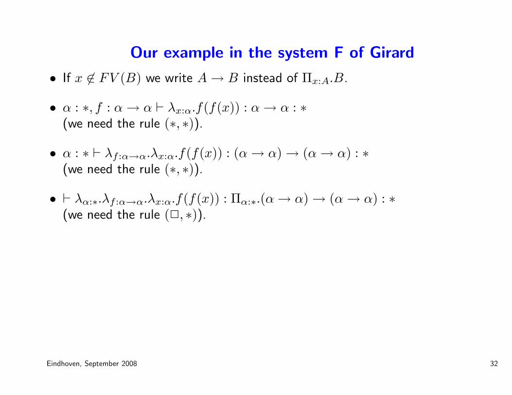
Our example in the system F of Girard

• If x 6∈ FV (B) we write A→ B instead of Πx:A.B.

• α : ∗, f : α→ α ⊢ λx:α.f(f(x)) : α→ α : ∗(we need the rule (∗, ∗)).

• α : ∗ ⊢ λf :α→α.λx:α.f(f(x)) : (α→ α)→ (α→ α) : ∗(we need the rule (∗, ∗)).

• ⊢ λα:∗.λf :α→α.λx:α.f(f(x)) : Πα:∗.(α→ α)→ (α→ α) : ∗(we need the rule (2, ∗)).


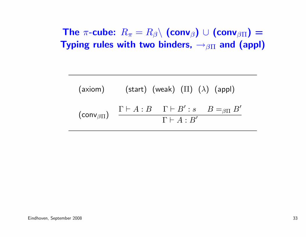
The π-cube: Rπ = Rβ\ (convβ) ∪ (convβΠ) =

Typing rules with two binders, →βΠ and (appl)

(axiom) (start) (weak) (Π) (λ) (appl)

(convβΠ)Γ ⊢ A : B Γ ⊢ B′ : s B =βΠ B′

Γ ⊢ A : B′


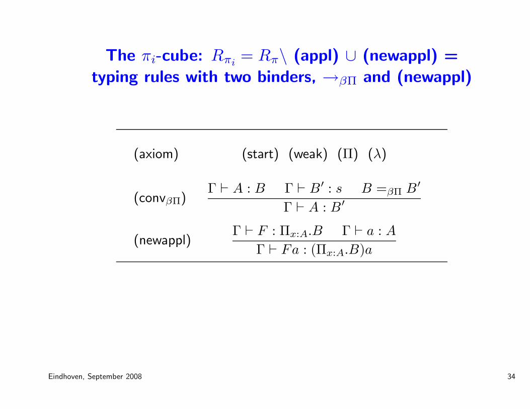
The πi-cube: Rπi= Rπ\ (appl) ∪ (newappl) =

typing rules with two binders, →βΠ and (newappl)

(axiom) (start) (weak) (Π) (λ)

(convβΠ)Γ ⊢ A : B Γ ⊢ B′ : s B =βΠ B′

Γ ⊢ A : B′

(newappl)Γ ⊢ F : Πx:A.B Γ ⊢ a : A

Γ ⊢ Fa : (Πx:A.B)a


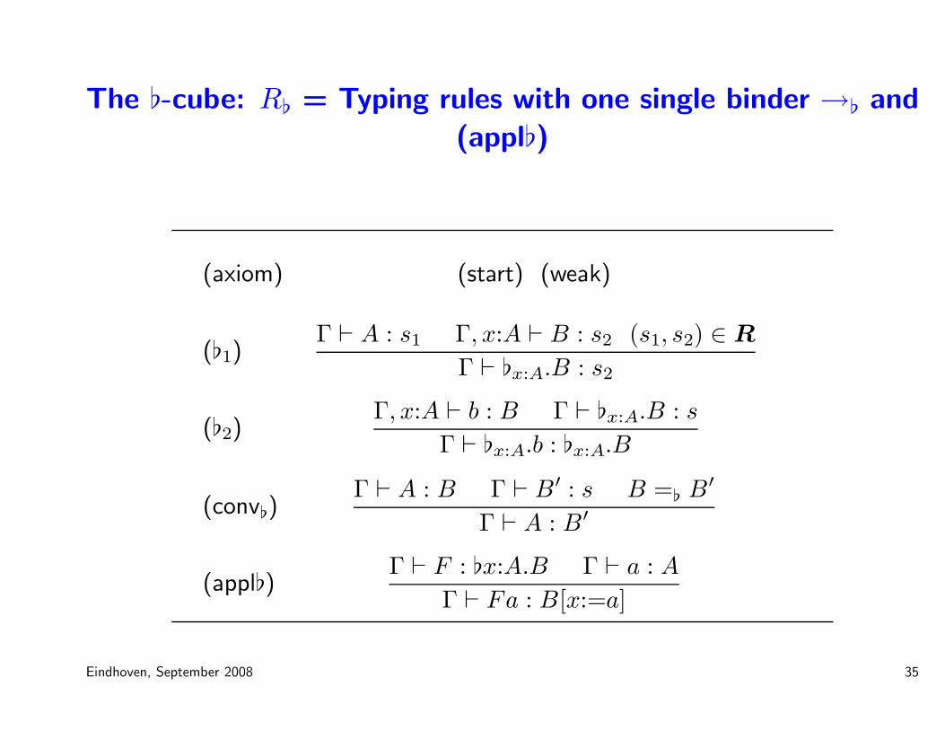
The ♭-cube: R♭ = Typing rules with one single binder →♭ and

(appl♭)

(axiom) (start) (weak)

(♭1)Γ ⊢ A : s1 Γ, x:A ⊢ B : s2 (s1, s2) ∈ R

Γ ⊢ ♭x:A.B : s2

(♭2)Γ, x:A ⊢ b : B Γ ⊢ ♭x:A.B : s

Γ ⊢ ♭x:A.b : ♭x:A.B

(conv♭)Γ ⊢ A : B Γ ⊢ B′ : s B =♭ B′

Γ ⊢ A : B′

(appl♭)Γ ⊢ F : ♭x:A.B Γ ⊢ a : A

Γ ⊢ Fa : B[x:=a]


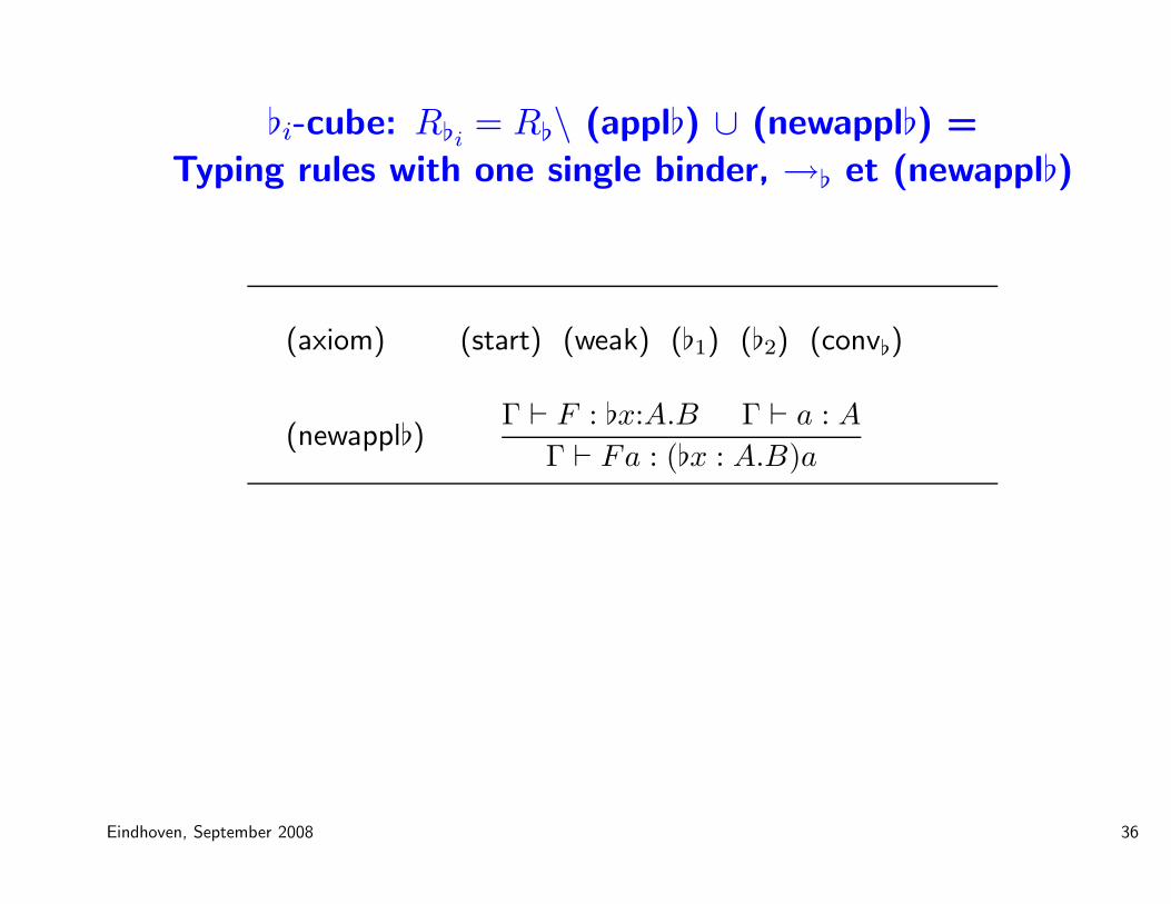
♭i-cube: R♭i= R♭\ (appl♭) ∪ (newappl♭) =

Typing rules with one single binder, →♭ et (newappl♭)

(axiom) (start) (weak) (♭1) (♭2) (conv♭)

(newappl♭)Γ ⊢ F : ♭x:A.B Γ ⊢ a : A

Γ ⊢ Fa : (♭x : A.B)a


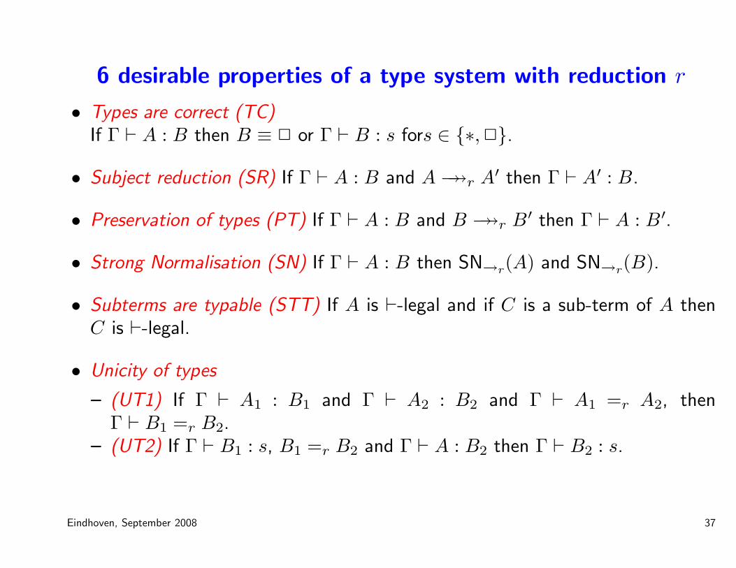
6 desirable properties of a type system with reduction r

• Types are correct (TC)If Γ ⊢ A : B then B ≡ 2 or Γ ⊢ B : s fors ∈ {∗, 2}.

• Subject reduction (SR) If Γ ⊢ A : B and A→→r A′ then Γ ⊢ A′ : B.

• Preservation of types (PT) If Γ ⊢ A : B and B →→r B′ then Γ ⊢ A : B′.

• Strong Normalisation (SN) If Γ ⊢ A : B then SN→r(A) and SN→r(B).

• Subterms are typable (STT) If A is ⊢-legal and if C is a sub-term of A thenC is ⊢-legal.

• Unicity of types

– (UT1) If Γ ⊢ A1 : B1 and Γ ⊢ A2 : B2 and Γ ⊢ A1 =r A2, thenΓ ⊢ B1 =r B2.

– (UT2) If Γ ⊢ B1 : s, B1 =r B2 and Γ ⊢ A : B2 then Γ ⊢ B2 : s.


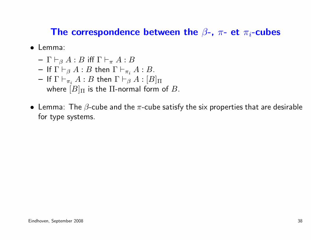
The correspondence between the β-, π- et πi-cubes

• Lemma:

– Γ ⊢β A : B iff Γ ⊢π A : B– If Γ ⊢β A : B then Γ ⊢πi

A : B.– If Γ ⊢πi

A : B then Γ ⊢β A : [B]Πwhere [B]Π is the Π-normal form of B.

• Lemma: The β-cube and the π-cube satisfy the six properties that are desirablefor type systems.


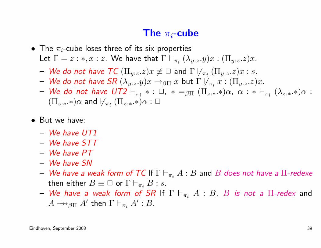
The πi-cube

• The πi-cube loses three of its six propertiesLet Γ = z : ∗, x : z. We have that Γ ⊢πi

(λy:z.y)x : (Πy:z.z)x.

– We do not have TC (Πy:z.z)x 6≡ 2 and Γ 6⊢πi(Πy:z.z)x : s.

– We do not have SR (λy:z.y)x→βΠ x but Γ 6⊢πix : (Πy:z.z)x.

– We do not have UT2 ⊢πi∗ : 2, ∗ =βΠ (Πz:∗.∗)α, α : ∗ ⊢πi

(λz:∗.∗)α :(Πz:∗.∗)α and 6⊢πi

(Πz:∗.∗)α : 2

• But we have:

– We have UT1– We have STT– We have PT– We have SN– We have a weak form of TC If Γ ⊢πi

A : B and B does not have a Π-redexethen either B ≡ 2 or Γ ⊢πi

B : s.– We have a weak form of SR If Γ ⊢πi

A : B, B is not a Π-redex andA→→βΠ A′ then Γ ⊢πi

A′ : B.


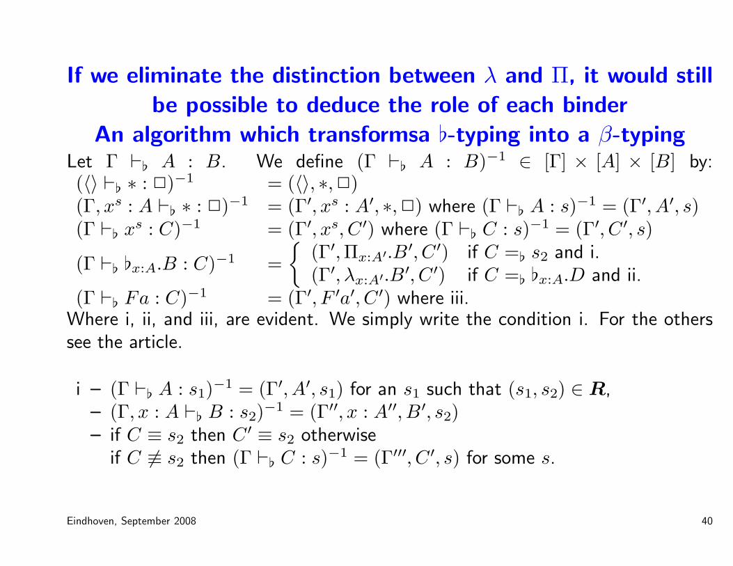
If we eliminate the distinction between λ and Π, it would still

be possible to deduce the role of each binder

An algorithm which transformsa ♭-typing into a β-typingLet Γ ⊢♭ A : B. We define (Γ ⊢♭ A : B)−1 ∈ [Γ] × [A] × [B] by:(〈〉 ⊢♭ ∗ : 2)−1 = (〈〉, ∗,2)(Γ, xs : A ⊢♭ ∗ : 2)−1 = (Γ′, xs : A′, ∗, 2) where (Γ ⊢♭ A : s)−1 = (Γ′, A′, s)(Γ ⊢♭ xs : C)−1 = (Γ′, xs, C′) where (Γ ⊢♭ C : s)−1 = (Γ′, C′, s)

(Γ ⊢♭ ♭x:A.B : C)−1 =

{

(Γ′,Πx:A′.B′, C′) if C =♭ s2 and i.(Γ′, λx:A′.B′, C′) if C =♭ ♭x:A.D and ii.

(Γ ⊢♭ Fa : C)−1 = (Γ′, F ′a′, C′) where iii.Where i, ii, and iii, are evident. We simply write the condition i. For the otherssee the article.

i – (Γ ⊢♭ A : s1)−1 = (Γ′, A′, s1) for an s1 such that (s1, s2) ∈ R,

– (Γ, x : A ⊢♭ B : s2)−1 = (Γ′′, x : A′′, B′, s2)

– if C ≡ s2 then C ′ ≡ s2 otherwiseif C 6≡ s2 then (Γ ⊢♭ C : s)−1 = (Γ′′′, C′, s) for some s.


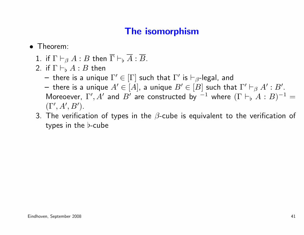
The isomorphism

• Theorem:

1. if Γ ⊢β A : B then Γ ⊢♭ A : B.2. if Γ ⊢♭ A : B then

– there is a unique Γ′ ∈ [Γ] such that Γ′ is ⊢β-legal, and– there is a unique A′ ∈ [A], a unique B′ ∈ [B] such that Γ′ ⊢β A′ : B′.Moreoever, Γ′, A′ and B′ are constructed by −1 where (Γ ⊢♭ A : B)−1 =(Γ′, A′, B′).

3. The verification of types in the β-cube is equivalent to the verification oftypes in the ♭-cube


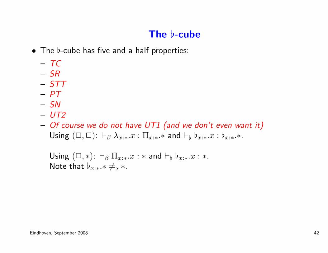
The ♭-cube

• The ♭-cube has five and a half properties:

– TC– SR– STT– PT– SN– UT2– Of course we do not have UT1 (and we don’t even want it)

Using (2,2): ⊢β λx:∗.x : Πx:∗.∗ and ⊢♭ ♭x:∗.x : ♭x:∗.∗.

Using (2, ∗): ⊢β Πx:∗.x : ∗ and ⊢♭ ♭x:∗.x : ∗.Note that ♭x:∗.∗ 6=♭ ∗.


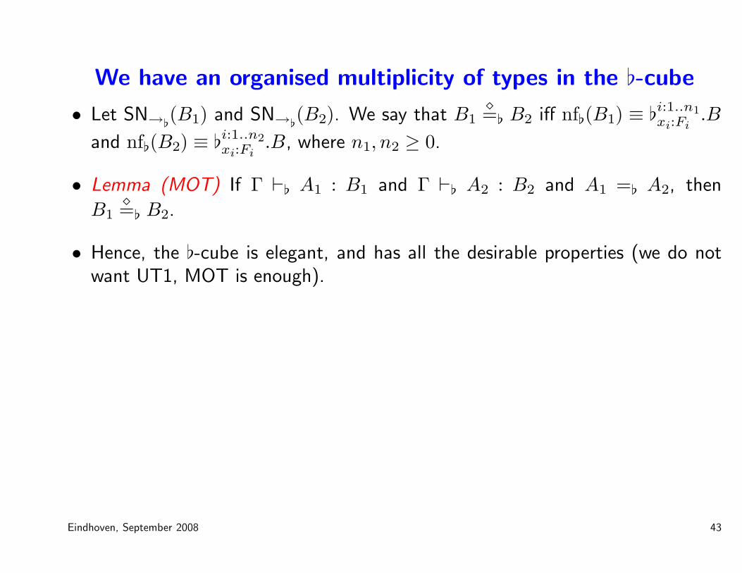
We have an organised multiplicity of types in the ♭-cube

• Let SN→♭(B1) and SN→♭

(B2). We say that B1⋄=♭ B2 iff nf♭(B1) ≡ ♭i:1..n1

xi:Fi.B

and nf♭(B2) ≡ ♭i:1..n2xi:Fi

.B, where n1, n2 ≥ 0.

• Lemma (MOT) If Γ ⊢♭ A1 : B1 and Γ ⊢♭ A2 : B2 and A1 =♭ A2, then

B1⋄=♭ B2.

• Hence, the ♭-cube is elegant, and has all the desirable properties (we do notwant UT1, MOT is enough).


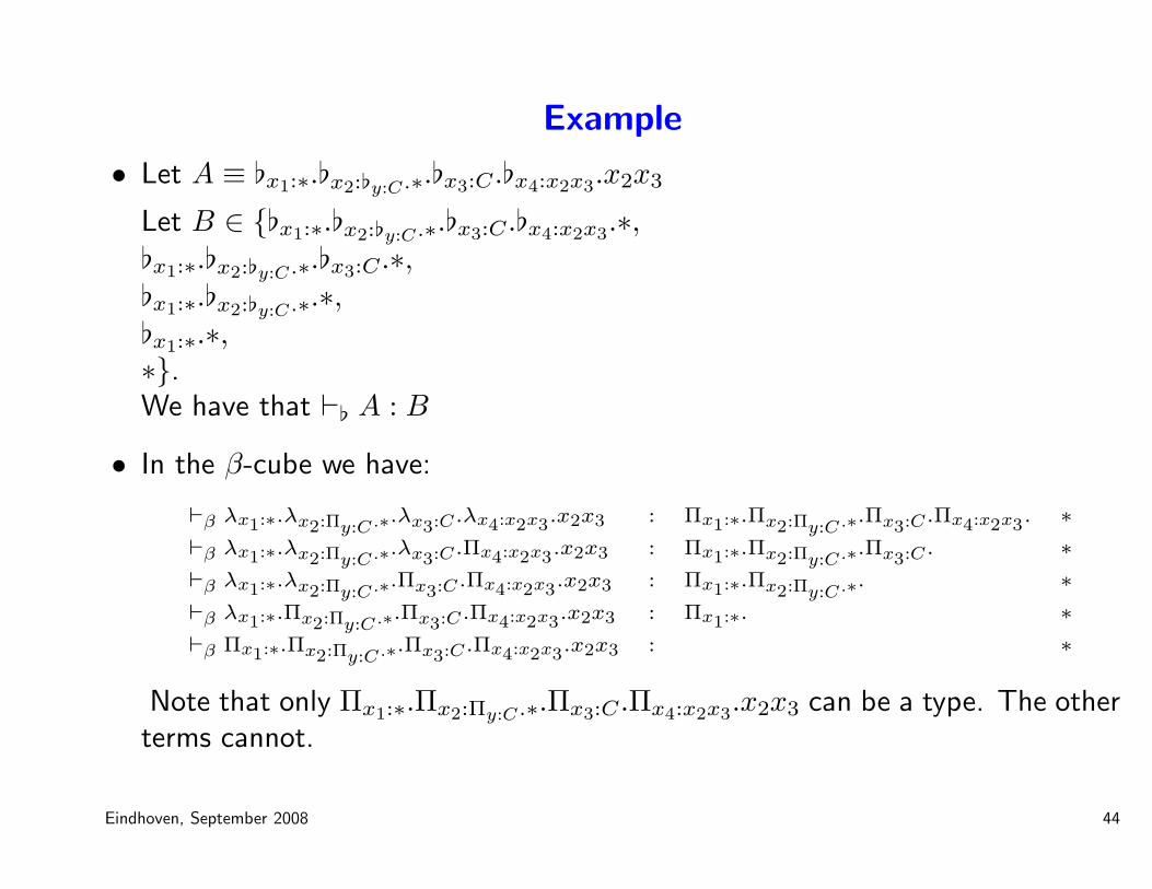
Example

• Let A ≡ ♭x1:∗.♭x2:♭y:C.∗.♭x3:C.♭x4:x2x3.x2x3

Let B ∈ {♭x1:∗.♭x2:♭y:C.∗.♭x3:C.♭x4:x2x3.∗,♭x1:∗.♭x2:♭y:C.∗.♭x3:C.∗,♭x1:∗.♭x2:♭y:C.∗.∗,♭x1:∗.∗,∗}.We have that ⊢♭ A : B

• In the β-cube we have:

⊢β λx1:∗.λx2:Πy:C.∗.λx3:C.λx4:x2x3.x2x3 : Πx1:∗.Πx2:Πy:C.∗.Πx3:C.Πx4:x2x3. ∗

⊢β λx1:∗.λx2:Πy:C.∗.λx3:C.Πx4:x2x3.x2x3 : Πx1:∗.Πx2:Πy:C.∗.Πx3:C. ∗

⊢β λx1:∗.λx2:Πy:C.∗.Πx3:C.Πx4:x2x3.x2x3 : Πx1:∗.Πx2:Πy:C.∗. ∗

⊢β λx1:∗.Πx2:Πy:C.∗.Πx3:C.Πx4:x2x3.x2x3 : Πx1:∗. ∗

⊢β Πx1:∗.Πx2:Πy:C.∗.Πx3:C.Πx4:x2x3.x2x3 : ∗

Note that only Πx1:∗.Πx2:Πy:C.∗.Πx3:C.Πx4:x2x3.x2x3 can be a type. The otherterms cannot.


Summary

• If the type system can do all that we want (as we have seen in the ♭-cube),why separate the levels of types and terms?

• Terms and types are not different. The only difference is the relation thatexists between them. In A : B, the A on the left represents a term, the B onthe right represents a type.

• Even if you do not want to use this system, its existence is already ofsignificance.


Conclusion

• There are still millions of hidden gems in de Bruijn’s Automath.

• Current work include de Bruijn’s subtyping, de Bruijn’s mathematicalvernacular.

• Is it an exageration to say that: “if an idea in logical frameworks is good, itexists already in Automath. Look enough you will find it.”

• Amazing that a single project (Automath) has resulted in such a treasure ofinfluential ideas.

• Thank you de Bruijn, and thanks to your extremely modest, and extremelyimpressive x-PhD students/researchers (Rob Nederpelt, Bert van BenthemJutting, Diedrick van Daalen, Herman Balsters, Jeff Zucker).

• What this group has done is truly impressive.


• I am particularly thankful to Rob Nederpelt who throughout decades hasintroduced me to the beautiful work in Automath and with whom I had mymost extensive collaboration (and a very close and valuable friendship).

• Keep studying Automath, and keep discovering its beauty.

• Long live de Bruijn and long live Automath.


Bibliography

Abadi, Cardelli, Curien, and Levy. The λσ calculus. Functional Programming, 1991.

Zena M. Ariola, Matthias Felleisen, John Maraist, Martin Odersky, and Philip Wadler. The call-by-need lambdacalculus. In Conf. Rec. 22nd Ann. ACM Symp. Princ. of Prog. Langs., pages 233–246, 1995.

Z.E.A. Benaissa, D. Briaud, P. Lescanne, and J. Rouyer-Degli. λυ, a calculus of explicit substitutions which preservesstrong normalisation. Journal of Functional Programming, 6(5):699–722, 1996.

Roel Bloo, Fairouz Kamareddine, and Rob Nederpelt. The Barendregt cube with definitions and generalisedreduction. Inform. & Comput., 126(2):123–143, May 1996.

N.G. de Bruijn. Generalising automath by means of a lambda-typed lambda calculus. 1984. Also in [Nederpelt et al.,1994], pages 313–337.

N.G. de Bruijn. Lambda calculus notation with nameless dummies, a tool for automatic formula manipulation, withapplication to the chuirch rosser theorem. In Indagationes Math, pages 381–392. 1972. Also in [Nederpelt et al.,

1994].

Philippe de Groote. The conservation theorem revisited. In Proc. Int’l Conf. Typed Lambda Calculi and Applications,

pages 163–178. Springer, 1993.


F. Kamareddine and A. Rıos. A λ-calculus a la de bruijn with explicit substitutions. Proceedings of ProgrammingLanguages Implementation and the Logic of Programs PLILP’95, Lecture Notes in Computer Science, 982:45–62,1995.

F. Kamareddine, R. Bloo, and R. Nederpelt. On Π-conversion in the λ-cube and the combination with abbreviations.Ann. Pure Appl. Logic, 97(1–3):27–45, 1999.

Fairouz Kamareddine. Postponement, conservation and preservation of strong normalisation for generalised reduction.

J. Logic Comput., 10(5):721–738, 2000.

Fairouz Kamareddine and Rob Nederpelt. Refining reduction in the λ-calculus. J. Funct. Programming, 5(4):637–651, October 1995.

Fairouz Kamareddine and Rob Nederpelt. A useful λ-notation. Theoret. Comput. Sci., 155(1):85–109, 1996.

Fairouz Kamareddine, Alejandro Rıos, and J. B. Wells. Calculi of generalised β-reduction and explicit substitutions:The type free and simply typed versions. J. Funct. Logic Programming, 1998(5), June 1998.

A. J. Kfoury and J. B. Wells. A direct algorithm for type inference in the rank-2 fragment of the second-order

λ-calculus. In Proc. 1994 ACM Conf. LISP Funct. Program., pages 196–207, 1994. ISBN 0-89791-643-3.

A. J. Kfoury and J. B. Wells. New notions of reduction and non-semantic proofs of β-strong normalization in typedλ-calculi. In Proc. 10th Ann. IEEE Symp. Logic in Comput. Sci., pages 311–321, 1995. ISBN 0-8186-7050-9.

URL http://www.church-project.org/reports/electronic/Kfo+Wel:LICS-1995.pdf.gz.


Assaf J. Kfoury, Jerzy Tiuryn, and Pawe l Urzyczyn. An analysis of ML typability. J. ACM, 41(2):368–398, March1994.

Rob Nederpelt. Strong Normalization in a Typed Lambda Calculus With Lambda Structured Types. PhD thesis,Eindhoven, 1973.

R.P. Nederpelt, J.H. Geuvers, and R.C. de Vrijer, editors. Selected Papers on Automath. Studies in Logic and the

Foundations of Mathematics 133. North-Holland, Amsterdam, 1994.

Laurent Regnier. Lambda calcul et reseaux. PhD thesis, University Paris 7, 1992.


(Typed) λ-Calculus and Formalising Mathematics `a la de Bruijn In … · 2010-10-07 · let...

Documents

Transcript of (Typed) λ-Calculus and Formalising Mathematics `a la de Bruijn In … · 2010-10-07 · let...