Two topics in R:Simulation and goodness-of-fit

HWU - GS

2

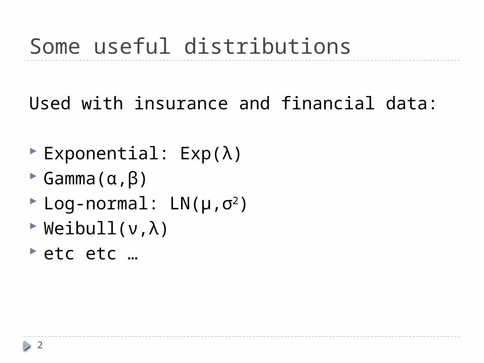
Some useful distributions

Used with insurance and financial data:

Exponential: Exp(λ) Gamma(α,β) Log-normal: LN(μ,σ2) Weibull(ν,λ) etc etc …

3

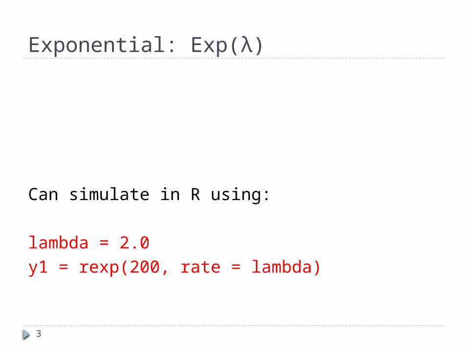
Exponential: Exp(λ)

Can simulate in R using:

lambda = 2.0

y1 = rexp(200, rate = lambda)

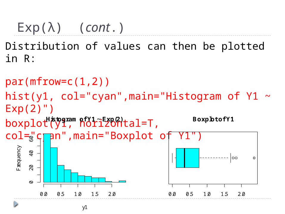
Exp(λ) (cont.)Distribution of values can then be plotted in R:

par(mfrow=c(1,2))

hist(y1, col="cyan",main="Histogram of Y1 ~ Exp(2)")

boxplot(y1, horizontal=T, col="cyan",main="Boxplot of Y1")

Histogram of Y1 ~ Exp(2)

y1

Fre

qu

en

cy

0.0 0.5 1.0 1.5 2.0

02

04

06

0

0.0 0.5 1.0 1.5 2.0

Boxplot of Y1

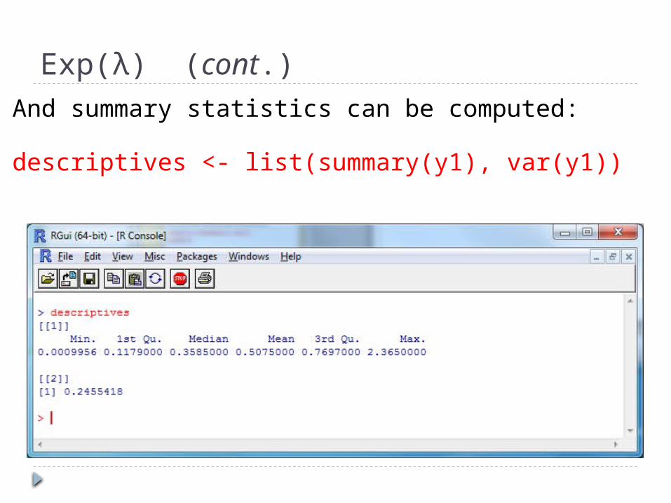
Exp(λ) (cont.)And summary statistics can be computed:

descriptives <- list(summary(y1), var(y1))

6

Gamma(α,β)

Can simulate in R using:

alpha = 3.0; beta = 2.0

y2 = rgamma(200, shape = alpha, rate = beta)

7

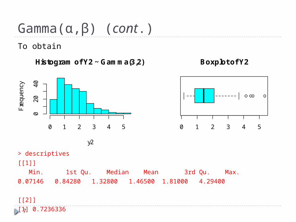
Gamma(α,β) (cont.)To obtain

> descriptives

[[1]]

Min. 1st Qu. Median Mean 3rd Qu. Max.

0.07146 0.84280 1.32800 1.46500 1.81000 4.29400

[[2]]

[1] 0.7236336

Histogram of Y2 ~ Gamma(3,2)

y2

Fre

qu

en

cy

0 1 2 3 4 5

02

04

0

0 1 2 3 4 5

Boxplot of Y2

8

Log-normal: LN(μ,σ2)

Note that

Can write a function in R that will return a generated sample together with plots and summary statistics.

9

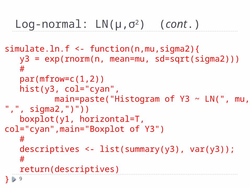
Log-normal: LN(μ,σ2) (cont.)

simulate.ln.f <- function(n,mu,sigma2){ y3 = exp(rnorm(n, mean=mu, sd=sqrt(sigma2))) # par(mfrow=c(1,2)) hist(y3, col="cyan", main=paste("Histogram of Y3 ~ LN(", mu, ",", sigma2,")")) boxplot(y1, horizontal=T, col="cyan",main="Boxplot of Y3") # descriptives <- list(summary(y3), var(y3)); # return(descriptives)}

10

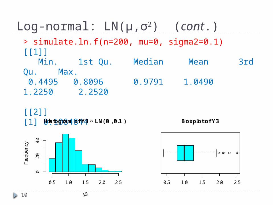
Log-normal: LN(μ,σ2) (cont.) > simulate.ln.f(n=200, mu=0, sigma2=0.1)

[[1]] Min. 1st Qu. Median Mean 3rd Qu. Max. 0.4495 0.8096 0.9791 1.0490 1.2250 2.2520

[[2]][1] 0.1084844

Histogram of Y3 ~ LN( 0 , 0.1 )

y3

Fre

qu

en

cy

0.5 1.0 1.5 2.0 2.5

02

04

0

0.5 1.0 1.5 2.0 2.5

Boxplot of Y3

11

Weibull(ν,λ)

R uses a different parameterisation, so we would better write our own code for simulating Weibull data.

12

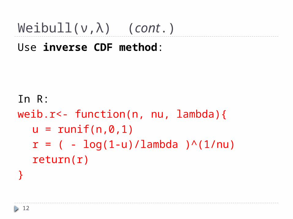
Weibull(ν,λ) (cont.)Use inverse CDF method:

In R:weib.r<- function(n, nu, lambda){

u = runif(n,0,1)

r = ( - log(1-u)/lambda )^(1/nu)

return(r)

}

13

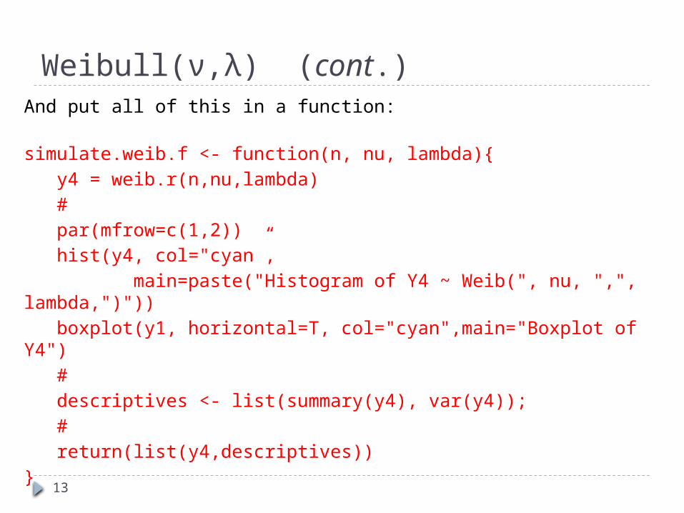
Weibull(ν,λ) (cont.)And put all of this in a function:

simulate.weib.f <- function(n, nu, lambda){

y4 = weib.r(n,nu,lambda)

#

par(mfrow=c(1,2))

hist(y4, col="cyan”,

main=paste("Histogram of Y4 ~ Weib(", nu, ",", lambda,")"))

boxplot(y1, horizontal=T, col="cyan",main="Boxplot of Y4")

#

descriptives <- list(summary(y4), var(y4));

#

return(list(y4,descriptives))

}

14

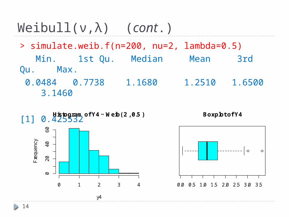
Weibull(ν,λ) (cont.)> simulate.weib.f(n=200, nu=2, lambda=0.5)

Min. 1st Qu. Median Mean 3rd Qu. Max.

0.0484 0.7738 1.1680 1.2510 1.6500 3.1460

[1] 0.425532

Histogram of Y4 ~ Weib( 2 , 0.5 )

y4

Fre

qu

en

cy

0 1 2 3 4

02

04

06

0

0.0 0.5 1.0 1.5 2.0 2.5 3.0 3.5

Boxplot of Y4

15

Goodness of fit

16

Empirical v theoretical CDF plot

Consider the Weibull(2, 0.5) example from before.

If the data are truly form this distn, then their empirical CDF should be close to the theoretical CDF of the Weibull(2, 0.5).

Plot these 2 in R and compare visually.

17

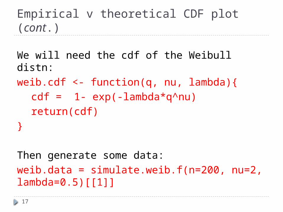
Empirical v theoretical CDF plot (cont.)

We will need the cdf of the Weibull distn:weib.cdf <- function(q, nu, lambda){

cdf = 1- exp(-lambda*q^nu)

return(cdf)

}

Then generate some data:weib.data = simulate.weib.f(n=200, nu=2, lambda=0.5)[[1]]

18

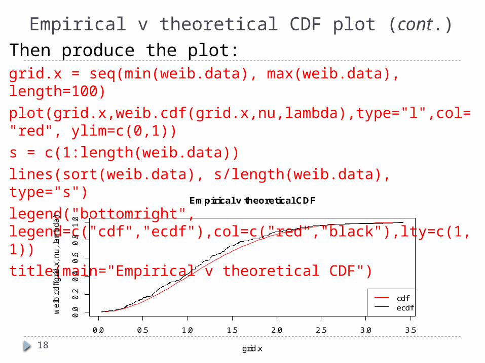
Empirical v theoretical CDF plot (cont.) Then produce the plot:grid.x = seq(min(weib.data), max(weib.data), length=100)

plot(grid.x,weib.cdf(grid.x,nu,lambda),type="l",col="red", ylim=c(0,1))

s = c(1:length(weib.data))

lines(sort(weib.data), s/length(weib.data), type="s")

legend("bottomright", legend=c("cdf","ecdf"),col=c("red","black"),lty=c(1,1))

title(main="Empirical v theoretical CDF")

0.0 0.5 1.0 1.5 2.0 2.5 3.0 3.5

0.0

0.2

0.4

0.6

0.8

1.0

grid.x

we

ib.c

df(

gri

d.x

, nu

, la

mb

da

)

Empirical v theoretical CDF

cdfecdf

19

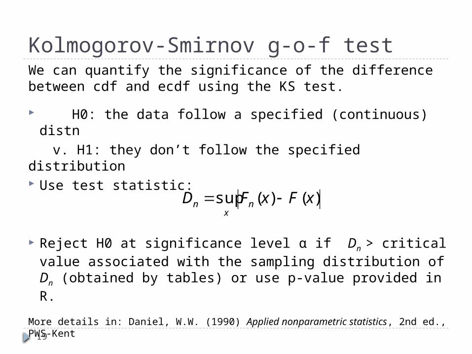
Kolmogorov-Smirnov g-o-f testWe can quantify the significance of the difference between cdf and ecdf using the KS test.

H0: the data follow a specified (continuous) distn v. H1: they don’t follow the specified distribution Use test statistic:

Reject H0 at significance level α if Dn > critical value associated with the sampling distribution of Dn (obtained by tables) or use p-value provided in R.

More details in: Daniel, W.W. (1990) Applied nonparametric statistics, 2nd ed., PWS-Kent

)()(sup xFxFD nx

n

20

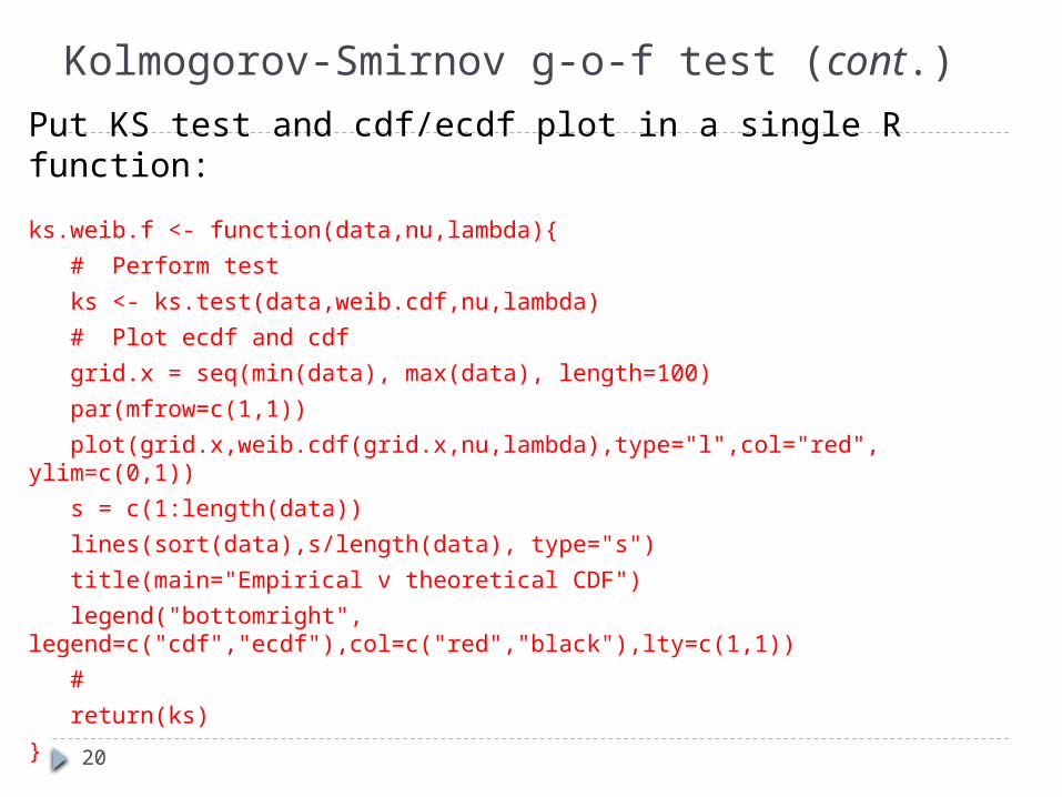
Kolmogorov-Smirnov g-o-f test (cont.)Put KS test and cdf/ecdf plot in a single R function:

ks.weib.f <- function(data,nu,lambda){

# Perform test

ks <- ks.test(data,weib.cdf,nu,lambda)

# Plot ecdf and cdf

grid.x = seq(min(data), max(data), length=100)

par(mfrow=c(1,1))

plot(grid.x,weib.cdf(grid.x,nu,lambda),type="l",col="red", ylim=c(0,1))

s = c(1:length(data))

lines(sort(data),s/length(data), type="s")

title(main="Empirical v theoretical CDF")

legend("bottomright", legend=c("cdf","ecdf"),col=c("red","black"),lty=c(1,1))

#

return(ks)

}

21

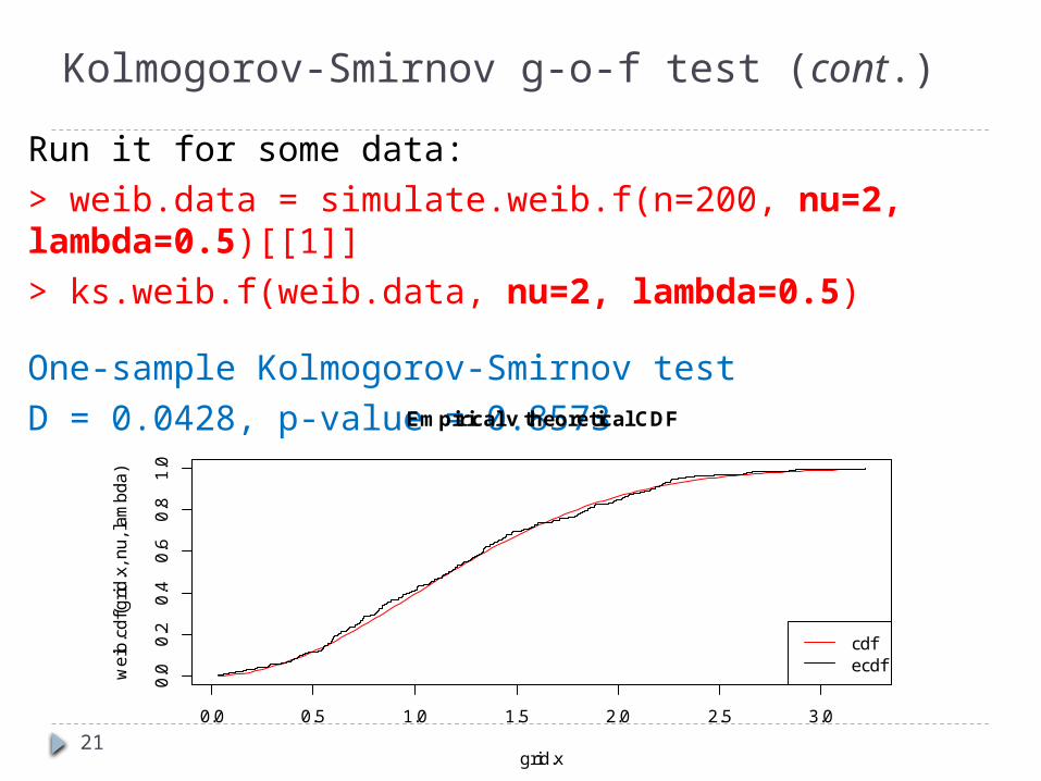
Kolmogorov-Smirnov g-o-f test (cont.)

Run it for some data:> weib.data = simulate.weib.f(n=200, nu=2, lambda=0.5)[[1]]

> ks.weib.f(weib.data, nu=2, lambda=0.5)

One-sample Kolmogorov-Smirnov test

D = 0.0428, p-value = 0.8573

0.0 0.5 1.0 1.5 2.0 2.5 3.0

0.0

0.2

0.4

0.6

0.8

1.0

grid.x

we

ib.c

df(

gri

d.x

, nu

, la

mb

da

)

Empirical v theoretical CDF

cdfecdf

22

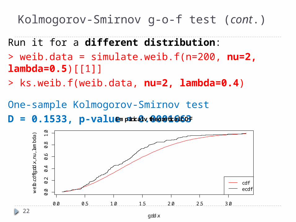
Kolmogorov-Smirnov g-o-f test (cont.)

Run it for a different distribution:> weib.data = simulate.weib.f(n=200, nu=2, lambda=0.5)[[1]]

> ks.weib.f(weib.data, nu=2, lambda=0.4)

One-sample Kolmogorov-Smirnov test

D = 0.1533, p-value = 0.0001663

0.0 0.5 1.0 1.5 2.0 2.5 3.0

0.0

0.2

0.4

0.6

0.8

1.0

grid.x

we

ib.c

df(

gri

d.x

, nu

, la

mb

da

)

Empirical v theoretical CDF

cdfecdf