The speed of sound in a magnetized hot Quark-Gluon-Plasma Based on: 0905.2097
−0.8 −0.6 −0.4 −0.2 0 0.2 0.4 0.6 0.8
−0.4
−0.2
0
0.2
0.4
0.6
0.8
x(λD)
y(λ
D)
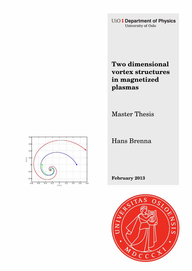
Two dimensionalvortex structuresin magnetizedplasmas
Master Thesis
Hans Brenna
February 2013

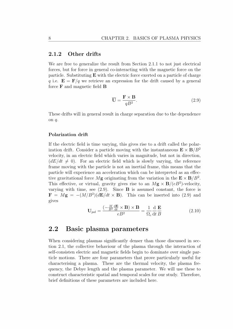
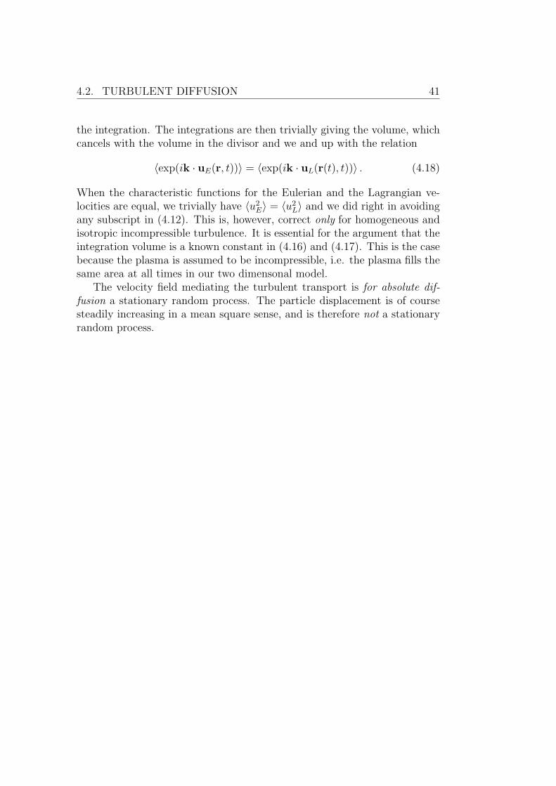
The figure on the front page shows the collapsing trajectories of threevortices with strengths γ1 = 2, γ2 = 2, γ3 = −1 at the positions (1/2, 0),(−1/2, 0) and
√3/2(cos(π/6), sin(π/6))


ii
Abstract
This thesis presents a numerical study of vortex structures in magnetizedplasmas. In a first approximation, such vortices can be understood as acollection of magnetic field aligned charged filaments. Their charge distri-bution gives rise to slowly varying E × B/B2-drifts of the ambient plasmaand the vortices embedded there. A mathematical model has been derived,studied analytically for low-dimensional vortex systems and implemented ascomputer code. The code has been verified by recreation of some of theanalytical results.
The main focus has been on the study of macroscopic structures createdby superimposing many discrete point vortex systems and on the study ofhomogeneous and isotropic vortex systems approximated by periodic bound-ary conditions. The dynamics of the structures show a wealth of phenomenafor relatively simple model, including long lived coherent formations and theevolution of stable tripolar macroscopic vortex systems from the collision oftwo vortex pairs. Homogeneous and isotropic vortex systems display the ba-sic properties of turbulent diffusion and transport, i.e. finite correlation time,continuous power spectra, etc. From these results we have calculated effec-tive diffusion coefficients for a range of vortex strengths and we have foundphenomenological relations between the Eulerian and Lagrangian integraltime scales and mean square velocities.
iii

iv

Acknowledgments
First of all, I would like to thank my supervisor, Prof. Hans Pecseli forgiving me this opportunity, for all your support and help during this project,and for reading my thesis innumerable times. It has been a great experienceworking with you!
I would also like to thank Vegard Lundby Rekaa for all his help with thewriting of my code. Thank you for taking your time to explain, and helpingme debug when I thought I had exhausted all options. Also, thank you forthe proofreading in the final stages.
And Prof. em. Jan Trulsen for his invaluable advise with the numericsand for helping me understand things I had never even thought of.
Thanks to Bjørn Lybekk for making several illustrations used in thisthesis.
Thanks to Anne Bregsaker, Elling Hauge-Iversen, Christoffer Stauslandand all the other students and staff at the Plasma and space physics forinteresting discussions and good times, during lunch and at times when oneshould work on one’s thesis.
And to I-M for making me think of other things occasionally.Finally I would like to thank everyone who has made me explain what I’ve
been doing this past year. Without failing to answer that question repeatedly,I would probably never have understood it myself.
v

vi
Contents
1 Introduction 11.1 Plasma . . . . . . . . . . . . . . . . . . . . . . . . . . . . . . . 11.2 Turbulence . . . . . . . . . . . . . . . . . . . . . . . . . . . . . 21.3 Motivation . . . . . . . . . . . . . . . . . . . . . . . . . . . . . 3
2 Basics of plasma physics 52.1 Single particle motion . . . . . . . . . . . . . . . . . . . . . . 5
2.1.1 The E×B-drift . . . . . . . . . . . . . . . . . . . . . . 52.1.2 Other drifts . . . . . . . . . . . . . . . . . . . . . . . . 8
2.2 Basic plasma parameters . . . . . . . . . . . . . . . . . . . . . 82.2.1 Thermal velocity . . . . . . . . . . . . . . . . . . . . . 92.2.2 The plasma frequency . . . . . . . . . . . . . . . . . . 92.2.3 The Debye length . . . . . . . . . . . . . . . . . . . . . 92.2.4 The plasma parameter . . . . . . . . . . . . . . . . . . 102.2.5 Summary . . . . . . . . . . . . . . . . . . . . . . . . . 10
2.3 Theoretical models . . . . . . . . . . . . . . . . . . . . . . . . 112.3.1 Single particle description . . . . . . . . . . . . . . . . 112.3.2 Kinetic description . . . . . . . . . . . . . . . . . . . . 122.3.3 Fluid description . . . . . . . . . . . . . . . . . . . . . 13
3 Flute modes 153.1 The vortex . . . . . . . . . . . . . . . . . . . . . . . . . . . . . 16
3.1.1 Electron Shielding . . . . . . . . . . . . . . . . . . . . 173.1.2 Some divergences . . . . . . . . . . . . . . . . . . . . . 18
3.2 Basic modes of propagation . . . . . . . . . . . . . . . . . . . 183.2.1 One vortex . . . . . . . . . . . . . . . . . . . . . . . . 183.2.2 Two vortices . . . . . . . . . . . . . . . . . . . . . . . . 183.2.3 Collision of two vortex pairs . . . . . . . . . . . . . . . 193.2.4 Collapse of three unshielded vortices . . . . . . . . . . 203.2.5 Hamiltonian property of vortex systems . . . . . . . . . 22
3.3 Many vortices . . . . . . . . . . . . . . . . . . . . . . . . . . . 24
vii
viii CONTENTS
3.3.1 Many vortices with deterministic positions . . . . . . . 24
3.4 Randomly distributed ensemble of vortices . . . . . . . . . . . 28
3.4.1 Localised cloud . . . . . . . . . . . . . . . . . . . . . . 28
3.4.2 Homogeneous ensembles . . . . . . . . . . . . . . . . . 28
3.5 Negative temperatures . . . . . . . . . . . . . . . . . . . . . . 28
3.5.1 Negative temperature states . . . . . . . . . . . . . . . 31
4 Turbulent diffusion and transport 33
4.1 Classical diffusion . . . . . . . . . . . . . . . . . . . . . . . . . 33
4.1.1 Diffusion of a light particle . . . . . . . . . . . . . . . . 34
4.2 Turbulent diffusion . . . . . . . . . . . . . . . . . . . . . . . . 35
4.2.1 Single particle diffusion . . . . . . . . . . . . . . . . . . 36
4.2.2 Eulerian and Lagrangian mean-square velocities . . . . 40
5 Numerical Model 43
5.1 Assumptions and approximations . . . . . . . . . . . . . . . . 43
5.1.1 Dimensions . . . . . . . . . . . . . . . . . . . . . . . . 44
5.2 Equations of motion . . . . . . . . . . . . . . . . . . . . . . . 44
5.2.1 Unshielded vortices . . . . . . . . . . . . . . . . . . . . 45
5.2.2 Shielded vortices . . . . . . . . . . . . . . . . . . . . . 45
5.2.3 Modified Bessel functions . . . . . . . . . . . . . . . . 46
5.3 4th order Runge-Kutta algorithm . . . . . . . . . . . . . . . . 46
5.4 Discretized equations of motion . . . . . . . . . . . . . . . . . 47
5.4.1 Initial conditions . . . . . . . . . . . . . . . . . . . . . 48
5.5 Time step . . . . . . . . . . . . . . . . . . . . . . . . . . . . . 48
5.5.1 Calculation of the Hamiltonian . . . . . . . . . . . . . 49
5.6 Test particles . . . . . . . . . . . . . . . . . . . . . . . . . . . 49
5.7 Eulerian points . . . . . . . . . . . . . . . . . . . . . . . . . . 50
5.8 Homogeneous systems . . . . . . . . . . . . . . . . . . . . . . 50
5.8.1 Periodic boundary conditions . . . . . . . . . . . . . . 50
6 Data analysis 53
6.1 Density histograms . . . . . . . . . . . . . . . . . . . . . . . . 53
6.2 Ensemble mean values . . . . . . . . . . . . . . . . . . . . . . 53
6.2.1 Schwarz’ inequality . . . . . . . . . . . . . . . . . . . . 54
6.3 Interpolation . . . . . . . . . . . . . . . . . . . . . . . . . . . 54
6.4 Correlation functions . . . . . . . . . . . . . . . . . . . . . . . 55
6.5 Probability density functions . . . . . . . . . . . . . . . . . . . 58
CONTENTS ix
7 Results 597.1 Time evolution of a localized random ensemble . . . . . . . . . 597.2 Collisions of four vortex clouds . . . . . . . . . . . . . . . . . . 707.3 Homogeneous systems . . . . . . . . . . . . . . . . . . . . . . 81
7.3.1 Constant vortex strengths . . . . . . . . . . . . . . . . 817.3.2 Varying vortex strength . . . . . . . . . . . . . . . . . 86
8 Discussions and Conclusions 918.1 Future perspectives . . . . . . . . . . . . . . . . . . . . . . . . 92
A C++ source code 99
B MATLAB data analysis routines 127

x CONTENTS
Chapter 1
Introduction
1.1 Plasma
A plasma is a state of matter where the atoms or molecules have been partlyor fully ionized, so that a portion of the ions and electrons can move aboutfreely. Plasma is in many ways similar to a gas, i.e. it will have no deter-mined volume or shape unless placed in a container. Under the influence ofelectric fields, the high conductivity of plasma leads flows of charged parti-cles generating currents and magnetic fields. Under the influence of magneticfields it can form structures such as filaments, rays and double layers.
In contrast with neutral gases, where the interactions between particlesare short range, long range interactions and forces due to electric and mag-netic fields are important in describing the properties and dynamics of plas-mas. This makes plasmas so different from gases that plasma is often calledthe fourth state of matter.
Plasma is the most common state of ordinary matter in the universe, over90% of it is in a plasma state, mainly in the intergalactic medium. Most ofthe visible matter is ionized as well, in stars. On Earth, plasma is muchless common and is usually associated with human activity, though lightningand other processes in thunder storms are known to produce plasma. Plasmais common, though in earth’s upper atmosphere, as well as near and outerspace. Because of the rarity of plasma phenomena on earth, it was notdiscovered until the 1870s by Sir William Crookes during his experiments onCrookes tubes (Crookes). Crookes used the term radiant matter for whathe observed; the term plasma was first used in 1928 by Irving Langmuir(Langmuir, 1928).
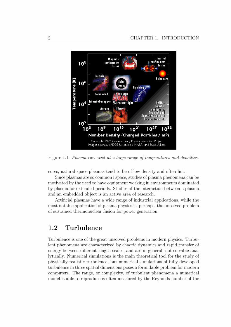
Figure 1.1 illustrated the range of temperatures and densities at whichplasmas can exist. Except for the plasmas in stars, and especially stellar
1
2 CHAPTER 1. INTRODUCTION
Figure 1.1: Plasma can exist at a large range of temperatures and densities.
cores, natural space plasmas tend to be of low density and often hot.
Since plasmas are so common i space, studies of plasma phenomena can bemotivated by the need to have equipment working in environments dominatedby plasma for extended periods. Studies of the interaction between a plasmaand an embedded object is an active area of research.
Artificial plasmas have a wide range of industrial applications, while themost notable application of plasma physics is, perhaps, the unsolved problemof sustained thermonuclear fusion for power generation.
1.2 Turbulence
Turbulence is one of the great unsolved problems in modern physics. Turbu-lent phenomena are characterized by chaotic dynamics and rapid transfer ofenergy between different length scales, and are in general, not solvable ana-lytically. Numerical simulations is the main theoretical tool for the study ofphysically realistic turbulence, but numerical simulations of fully developedturbulence in three spatial dimensions poses a formidable problem for moderncomputers. The range, or complexity, of turbulent phenomena a numericalmodel is able to reproduce is often measured by the Reynolds number of the
1.3. MOTIVATION 3
initial flow. The range, or complexity, of turbulent phenomena a numeri-cal model is able to reproduce is often measured by the Reynolds numberof the initial flow. Some of the largest present day simulations thus assumeReynolds numbers∼ 500 or even less; compared to∼ 5000 (Frisch, 1996) thatcan be quite easily obtained in turbulent pipe flows. It can have great valueto find simpler, yet physically realistic and realisable models, that requirereduced computer resources. Such models can then be used as a “test-bed”for ideas of general interest, such as the Eulerian-Lagrangian transformationof time scales or correlation functions, detailed investigations of parametervariations of turbulent diffusion, etc. Simulations in two dimensions, as ad-dressed in the present study, offer such a possibility.
1.3 Motivation
In this thesis , we will first discuss general plasma phenomena (scales, sin-gle particle motions, kinetic and fluid models) in Chapter 2. We will thenintroduce flute modes and turbulent diffusion as the theoretical frameworkneeded to analyse the results we present later. Next we present the numer-ical methods developed for this thesis in Chapter 5 and the data analysismethods in Chapter 6. Last we present the results in Chapter 7 and someconcluding remarks in Chapter 8.
The main goals of this thesis are:
The derivation and description of a simple, yet realistic, model forthe low frequency dynamics of homogeneously magnetized plasmas;formulated in terms of interacting line vortices.
The implementation of this model in a computer program.
The utilisation of the program to run simulations of physically relevantsystems.
Demonstrate that vortex systems can develop characteristics similar toturbulent flows, i.e. correlation functions with finite memory (correla-tion times) and continuous power spectra.
Use numerical results to illustrate basic results for particle transportdue to random or turbulent motions.

4 CHAPTER 1. INTRODUCTION
Chapter 2
Basics of plasma physics
2.1 Single particle motion
A good starting point for our discussion of basic plasma physics is the dynam-ics and behaviour of single particles interacting with electric and magneticfields. Many of the drifts and phenomena described here are important asbulk movements in plasmas consisting of many particles, especially if theplasma is dilute.
2.1.1 The E×B-drift
The force on a charged particle in an electric and a magnetic field is givenby the Lorentz force
F = q(E + U×B). (2.1)
where F is the force on a particle with charge q due to the electric field Eand the magnetic field B and U is the velocity of the particle.
Consider a single particle with massmmoving in a uniform and stationarymagnetic field with velocity U. Assuming E = 0 the equation of motion forthis particle is then
md
dtU⊥ = qU⊥ ×B, (2.2)
where U⊥ is the components of the velocity which are perpendicular to B.Since the magnetic force on a particle is always perpendicular to the velocity,magnetic forces alone can neither add, nor transfer, energy to or from theparticle, only change the direction of the velocity. The result is a gyratingmotion of the particle in a circular orbit with radius
rL =mU⊥qB
, (2.3)
5
6 CHAPTER 2. BASICS OF PLASMA PHYSICS
where rL is known as the Larmor radius with corresponding frequency
Ωc =qB
m(2.4)
also referred to as the cyclotron frequency.Consider the case where we have a constant electric field in the direction
perpendicular to B, the magnetic field still being constant in space and time.The equations of motion in the direction perpendicular to B becomes
md
dtU⊥ = q(E⊥ + U⊥ ×B) (2.5)
We know that by a suitable change of reference the electric field can be madeto vanish. We introduce a new velocity U∗ = U⊥−E⊥×B/B2, where U⊥ isthe “true“ particle velocity. Substituting this new velocity into the equationof motion correspond to changing the frame of reference to the one in whichthe electric field is vanishing. The velocity U∗ thus follows the equation
md
dtU∗(t) = qU∗(t)×B. (2.6)
In this frame of reference we have a gyro-orbit solution for U∗(t), as inequation 2.2. The actual trajectory is obtained by changing reference systemback to the laboratory frame by adding the velocity
UE×B =E×B
B2(2.7)
generally called the E×B-velocity. This will be an average velocity associatedwith the gyro-centre, in addition to the circular gyrating motion. The realtrajectory will thus be a type of curve called a cycloid.
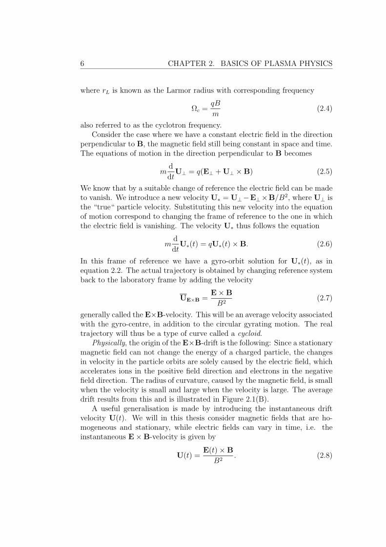
Physically, the origin of the E×B-drift is the following: Since a stationarymagnetic field can not change the energy of a charged particle, the changesin velocity in the particle orbits are solely caused by the electric field, whichaccelerates ions in the positive field direction and electrons in the negativefield direction. The radius of curvature, caused by the magnetic field, is smallwhen the velocity is small and large when the velocity is large. The averagedrift results from this and is illustrated in Figure 2.1(B).
A useful generalisation is made by introducing the instantaneous driftvelocity U(t). We will in this thesis consider magnetic fields that are ho-mogeneous and stationary, while electric fields can vary in time, i.e. theinstantaneous E×B-velocity is given by
U(t) =E(t)×B
B2. (2.8)
2.1. SINGLE PARTICLE MOTION 7
Figure 2.1: Illustration of single particle drifts in a homogeneous mag-netic field. (A) No disturbing force, (B) a homogeneous electric field,(C) an independent homogeneous force, e.g. a gravitational field, (D)an inhomogeneity in the magnetic field. Image created by Ian Tresman.Source:http://commons.wikimedia.org/wiki/File:Charged-particle-drifts.svg
8 CHAPTER 2. BASICS OF PLASMA PHYSICS
2.1.2 Other drifts
We are free to generalize the result from Section 2.1.1 to not just electricalforces, but for force in general co-interacting with the magnetic force on theparticle. Substituting E with the electric force exerted on a particle of chargeq i.e. E = F/q we retrieve an expression for the drift caused by a generalforce F and magnetic field B
U =F×B
qB2. (2.9)
These drifts will in general result in charge separation due to the dependenceon q.
Polarization drift
If the electric field is time varying, this gives rise to a drift called the polar-ization drift. Consider a particle moving with the instantaneous E ×B/B2
velocity, in an electric field which varies in magnitude, but not in direction,(dE/dt 6= 0). For an electric field which is slowly varying, the referenceframe moving with the particle is not an inertial frame, this means that theparticle will experience an acceleration which can be interpreted as an effec-tive gravitational force Mg originating from the variation in the E×B/B2.This effective, or virtual, gravity gives rise to an Mg × B/(eB2)-velocity,varying with time, see (2.9). Since B is assumed constant, the force isF = Mg = −(M/B2)(dE/dt × B). This can be inserted into (2.9) andgives
Upol =(−M
B2dEdt×B)×B
eB2=
1
Ωc
d
dt
E
B(2.10)
2.2 Basic plasma parameters
When considering plasmas significantly denser than those discussed in sec-tion 2.1, the collective behaviour of the plasma through the interaction ofself-consisten electric and magnetic fields begin to dominate over single par-ticle motions. There are four parameters that prove particularly useful forcharacterising a plasma. These are the thermal velocity, the plasma fre-quency, the Debye length and the plasma parameter. We will use these toconstruct characteristic spatial and temporal scales for our study. Therefore,brief definitions of these parameters are included here.
2.2. BASIC PLASMA PARAMETERS 9
2.2.1 Thermal velocity
The thermal velocity is the typical velocity of the thermal motion of theparticles in a fluid or gas of a given temperature. The definition used here is
uth,s =
(κTsms
)1/2
, (2.11)
where κTs is the temperature and ms is the mass of particle species s. Anumerical constant has been omitted from the definition for simplicity.
2.2.2 The plasma frequency
Consider a slab of plasma with the electron displaced slightly with respectto the ions. This small perturbation in the charge distribution sets up anelectric field trying to restore the imbalance. Since the electrons are muchlighter, and hence more mobile than the ions, the electrons start to oscillatearound the equilibrium position with the characteristic frequency
ωpe =
(e2n
ε0me
)1/2
(2.12)
where n is the number density and me is the electron mass. The correspond-ing plasma period is the τp = 2π/ωpe.
2.2.3 The Debye length
The Debye length λD characterises a shielding distance. When a surplusparticle with charge q is introduced into a plasma, the surrounding plasmareorganizes in an attempt to screen off the electric potential arising from thecharge q. The result is that at larger distances from the perturbing charge,the perturbation is close to undetectable and only the collective behaviourof all the particles can be observed. At distance λD from the charge q, theelectric potential of this charge is reduced by a factor e−1: The charge isshielded by the surrounding plasma. The Debye length is defined as
λD =
(ε0κT
e2n
)1/2
. (2.13)
A plasma particle travelling with the thermal velocity will travel one Debyelength in one plasma period.
10 CHAPTER 2. BASICS OF PLASMA PHYSICS
2.2.4 The plasma parameter
From the Debye length and the plasma density the plasma parameter can beconstructed as
Np = nλ3D. (2.14)
This dimensionless quantity is, apart from a factor of order unity, the averagenumber of particles within a sphere with radius λD. For large Np, a smallperturbation in the plasma will not be noticed at large distances, since thesurrounding plasma efficiently screens off the perturbation and the overallelectric field is not noticeably influenced. If, on the other hand, Np is low,any perturbation can have a significant effect on the surroundings. Plasmaswith large Np can for most purposes be considered to be collisionless and thedynamics are controlled by collective interactions.
Note that the plasma parameter actually decreases for increasing n assum-ing constant temperature, since λ3
D ∼ n−3/2T 3/2, we have Np ∼ n−1/2T 3/2.Plasmas with large Np thus have low density and high temperature, and arecharacterised as hot and dilute.
Note also that the plasma parameter as defined here only makes physicalsense in three spatial dimensions. Since our main concern in this study istwo dimensional plasmas, the plasma parameter has to be redefined as thenumber of particles in a rectangle with area λ2
D.
2.2.5 Summary
Even though the parameters we have introduced here are constructed with anelectron gas or electron dynamics as examples, it is straight forward to con-struct similar quantities for gases of different species and for mixed chargedgases. In the latter example, different species are allowed to have differenttemperatures, densities, etc.
For the vortex structures introduced in the next chapter including themodel and corresponding assumptions used, the thermal velocity and theplasma frequency are with limited physical significance. Instead the magni-tude of the E × B/B2-velocity will serve as a characteristic velocity U0 =E0/B0. The Debye length will still be used as a characteristic distance,and from combining the latter we can construct the characteristic time scalet0 = λD/U0 as the time a particle travelling with velocity U0 takes to travelone Debye length.
2.3. THEORETICAL MODELS 11
2.3 Theoretical models
From the discussion so far, we can conclude that the motion of any chargedparticle in the presence of electric and magnetic fields will be governed bythe Lorentz’ force
F(Xj, t) = qj(E(Xj, t) + Uj(t)×B(Xj, t)), (2.15)
where all fields are assumed to be functions of both position and time, e.g.B = B(X(t), t), and Xj = Xj(t), Vj = Vj(t), qj are the position, velocityand charge of particle j. The magnetic and electric fields are given selfconsistently from Maxwell’s equations
∇ · E =ρ
ε0
, (Gauss’ law for electric fields) (2.16)
∇ ·B = 0, (Gauss’ law for magnetic fields) (2.17)
∇× E = −∂B
∂t, (Faraday’s law) (2.18)
∇×B = µ0j + µ0ε0∂E
∂t, (The modified Ampere law) (2.19)
where ρ is the plasma charge density, j is the current density and ε0, µ0 isthe vacuum permeability and susceptibility respectively. In all cases studiedin this thesis the electric field will be assumed to be electrostatic, so E =−∇φ, and by substitution, Gauss’ law for electric fields simplifies to Poisson’sequation
∇2φ = − ρε0. (2.20)
2.3.1 Single particle description
Through integrating the equations of motion, a set of equations describingthe trajectories of an ensemble N of particles can be retrieved, all of whichare to be solved together with Maxwell’s equations (2.16)-(2.19),
dXj
dt= Uj (2.21)
dUj
dt=
Fj
mj
=qjmj
(E(Xj, t) + Uj(t)×B(Xj, t)) (2.22)
ρ =
∫qjN(x,u, t)dv (2.23)
j =
∫qjvN(x,u, t)dv (2.24)
12 CHAPTER 2. BASICS OF PLASMA PHYSICS
where N(x,v, t) =∑
j δ(x−Xj(t))δ(v−Vj(t)) is the density of particles inphase space.
Attempting to solve these equations fully for the ensemble N involvessolving equations (2.21)-(2.24) N 2 times, a task which is in most cases al-most impossible to perform numerically, let alone analytically. The challengeof solving such a problem is often referred to as the N-body problem and themethod in general molecular dynamics. Here, it is worth mentioning the no-tation often used in numerical simulations, the order or complexityO(N 2) fora given number of particles N . Though computationally difficult to perform,the method has relevance to this thesis.
This single particle description, which explicitly keeps track of every sin-gle component particle in the plasma is, luckily, more detailed than usuallyneeded, and there are two approximative descriptions of plasma dynamicsthat are widely used, and will be discussed in the remainder of this chapter..
2.3.2 Kinetic description
The first approximation is achieved by introducing the probability distribu-tion function
f(x,v, t) = 〈N(x,v, t)〉 (2.25)
where 〈...〉 represents the ensemble average over over all realisations of theplasma consistent with give constraints. By assuming that the exact solutionscan be expanded in terms of a distribution and a correction to account forthe two-particle interactions (collisions), we get the plasma kinetic equation.Assuming no collisions the kinetic equation simplifies to the Vlasov equation
∂f(x,v, t)
∂t+ v · ∇xf(x,v, t) +
q
mE(x, t) + v ×B(x, t) = 0 (2.26)
which describes the time evolution of a plasma. For the probability densityfunctions f(x,v, t) to represent a probabilistically acceptable system thereare some requirements that need to be met:
f(x,v, t) ≥ 0 for all x,v, t.
Integrating f(x,v, t) over all physical space and velocity space givesthe total number of particles.
f(x,v, t)→ 0 for v → ±∞.
The kinetic description has it’s strengths in that it allows us to reduce thecomplexity of the problem without loosing all detailed information. It’sstrongest limitation is the assumption of no collisions, which in most space-and astrophysical problems, is after all a good approximation.
2.3. THEORETICAL MODELS 13
2.3.3 Fluid description
The fluid description of plasmas is even further removed from the single par-ticle description, in that the fluid description only considers the bulk densityand the bulk velocity, and as such describes the plasma as an electricallycharged fluid. The quantities kept are the particle density, charge density,bulk velocity and charge density defined as:
n = n(x, t) =∑s
ns =∑s
∫fs(x,v, t)dv, (2.27)
ρe = ρe(x, t) =∑s
qsns =∑s
qs
∫fs(x,v, t)dv, (2.28)
nu = n(x, t)u(x, t) =∑s
nsus =∑s
∫vfs(x,v, t)dv, (2.29)
j = j(x, t) =∑s
qsnsus (2.30)
where s represents the particle species involved.The fluid description can be derived from the kinetic description by mul-
tiplying the Vlasov equation with m, mv and mvv and then integratingover velocity space. Thus gives the fluid equations for conservation of mass,momentum and energy:
∂ρ
∂t+∇ · (ρu) = 0 (2.31)
ρ
(∂u
∂t+ u · ∇u
)= ρe(E + u×B)−∇p (2.32)
∂
∂t
(ρu2
2+
3p
2
)+∇ ·
(ρu2u
2+
3pu
2
)= j · E−∇ · (ρu). (2.33)
Here ρ = nm is mass density, p, ρu2/2 and 3p/2 are the plasma pressure,kinetic energy and thermal energy, respectively, and ρe is the charge den-sity. By combining equations (2.31)-(2.33) with Maxwell’s equations and anequation of state, we have a closed set of equations which can be solved fora given plasma.
The most commonly used fluid plasma model, magnetohydrodynamics(MHD), treats the plasma as a single fluid, which makes charge separationimpossible. There are different ways of omitting this limitation in fluid mod-els, the simplest of which decscribe the plasma as consisting of multiplefluids, one for each particle specie. This allows for charge separation, but isgenerally more complicated.

14 CHAPTER 2. BASICS OF PLASMA PHYSICS
Chapter 3
Flute modes
Flute modes are a limiting case of electrostatic plasma perturbations whereall of (or almost all) spatial variations of the potential is in the directionperpendicular to the magnetic field B. This limit can be derived form amore general three dimensional plasma model.
First we introduce the continuity equation
∂ne∂t
+∇ · neUe = 0 (3.1)
for the electrons, and∂ni∂t
+∇ · niUi = 0 (3.2)
for the ions; and the momentum equations
mene
(∂Ue
∂t+ Ue · ∇ ·Ue
)= −∇p− ene (E + Ue ×B) (3.3)
for the electrons and
mini
(∂Ui
∂t+ Ui · ∇ ·Ui
)= −∇p+ eni (E + Ui ×B) (3.4)
for the ions.Assuming that the only bulk flow is due to the E×B-drift, we have the
bulk velocity in the form U = −∇⊥φ×BB2 since the electric field is electrostatic.
In the electrostatic limit the particle species are linked through Poisson’sequation
∇2φ =e
ε0
(ne − ni). (3.5)
Note that U defined before is the same for both electron and ion guidingcentres. Note also that the flow is incompressible for B = constant, i.e.∇ ·U = 0 since ∇× (∇φ×B) = 0 here.
15
16 CHAPTER 3. FLUTE MODES
Taking (3.1)-(3.2), using Poisson’s equation and assuming the same in-compressible flow for both species, where we identify the particle positionwith the guiding centre position, we obtain the equation(
∂
∂t− 1
B2∇⊥φ×B · ∇⊥
)∇2φ = 0 (3.6)
which uniquely determines the evolution of the electrostatic potential whenan initial condition is given. This equation is inherently non-linear sincelinearisation gives trivially ∂φ
∂t= 0.
Taking (3.1)+(3.2) gives an equation for the evolution of the bulk plasmadensity (
∂
∂t− 1
B2∇⊥φ×B · ∇⊥
)n = 0 (3.7)
with n ≡ 12(ne + ni) and φ is assumed given from solving 3.6. This equation
determines the evolution of the entire plasma density once the potential isgiven.
3.1 The vortex
In fluid mechanical potential theory, a point vortex is a two-dimensionalstructure characterized by a velocity potential on the form
Φ = γ ln r (3.8)
in two spatial dimensions. This corresponds to a so-called irrotational circu-lation with ∇×U = 0, where the streamlines are concentric circles and thevelocity is proportional to 1/r. A line charge, i.e. an infinitely long line ofcharge, with constant density will have the electrostatic potential distribution
φ =Q
2πε0
ln r. (3.9)
By superimposing a homogeneous magnetic field B, the E ×B/B2 velocityin the plasma will be
Ur, Uθ, Uz =Q
2πε0B
0,
1
r, 0
(3.10)
in cylindrical coordinates where we introduced E = −∇φ. This potential isan exact non-linear solution of equations (3.6) and (3.7) and corresponds to”charging-up” of a magnetic field line. The result is a non-uniform rotation
3.1. THE VORTEX 17
of the entire plasma around the charge distribution. The angular directionof the rotation changes with the sign of the charge or the magnetic field.The resulting velocity field is equivalent to a point vortex. Throughout thisthesis, such line charge structures will routinely be referred to as vortices.
By this model we represent a charge by an idealized “line“ distribution.For a physically more realistic case, we have to assume a finite line widthgiven by an average Larmor radius of the particle species in question.
3.1.1 Electron Shielding
The vortex defined above, assumes that all line charges are perfectly alignedto the magnetic field. By relaxing this assumption, and allowing pertur-bations to make a small angle with respect to the magnetic field, the ionswill still be bound to the magnetic field, but the electrons can flow alongthe field lines to maintain an isothermal Boltzmann distribution ne(r, t) =n0 exp(eφ(r, t)/κTe). We denote this as a “quasi two dimensional” limit. De-scribing the ions in two dimensions while allowing the electrons to move inthis way is consistent as long as the transverse ion E⊥ ×B-velocity is muchlarger than the ion velocity V|| ∼ eE/(ωM) along B.
By using Poisson’s equation on the form
∇2⊥φ =
e
ε0
(en0φ
κTe− ni
)(3.11)
electron shielding can be accounted for. Here the Boltzmann distribution islinearised and the ion density is ni = n0 − ni. Combining this with the ioncontinuity equation and the ion velocity −∇φ×B/b2 gives[
∂
∂t− 1
B2∇⊥φ×B · ∇⊥
](∇2⊥φ−
1
λ2D
φ
)= 0 (3.12)
which is identical to
∂
∂t
(∇2φ− 1
λ2D
)− 1
B2(∇⊥φ×B · ∇⊥)∇2
⊥φ = 0 (3.13)
where the Debye length enters as a shielding distance.An exact solution to this is again a line charge, but now with a different
radial potential distribution. The shielded vortex will have a potential of theform φ(r) = aK0(r) where K0 is the modified Bessel function of the secondkind.
These shielded vortices will behave differently, in that their interactionsare basically limited in distance to the electron Debye length of the plasma inwhich they are embedded (See Section 2.2.3 for a discussion of the physicalmeaning of the Debye length.).
18 CHAPTER 3. FLUTE MODES
3.1.2 Some divergences
The vortex is inertia-less in the sense defined here, and we will not define akinetic energy density associated with it, in the usual sense. (We consideran effective Hamiltonian later.) It may still be interesting to note, howeverthat
∫∞0u2dr →∞.
3.2 Basic modes of propagation
By introducing the centre of vorticity as defined by Aref (1979) we can studythe motion of a configuration of more than one vortex. The centre of vorticityis given as
(X, Y ) =1∑α γα
(∑α
γαxα,∑α
γαyα
)(3.14)
where γα is the strength of vortex α, in our case γα = Qα2πε0
, and (xα, yα)is the position of vortex α
3.2.1 One vortex
The motion of one vortex is trivial, since it can not induce motion on itself.
3.2.2 Two vortices
The simplest non-trivial case is to consider two vortices separated by a dis-tance l along, say, the y-axis, with the vortices in the positions y = ±l/2.Their motion can then be classified into the four different cases Q1 = Q2 = Q,Q1 = −Q2, Q1 > 0, Q2 > 0 and Q1 > 0, Q2 < 0 by the position of theircentres of vorticity.
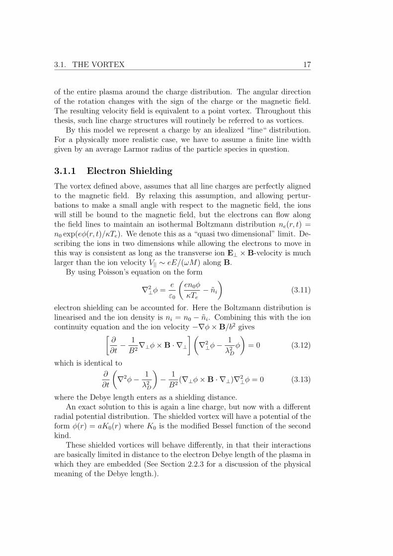
In the first case, the centre of vorticity will be in (0, 0) and the vorticeswill convect each other in opposite directions, and the result will be a circularmotion without net displacement. This case is illustrated in figure 3.1(a).
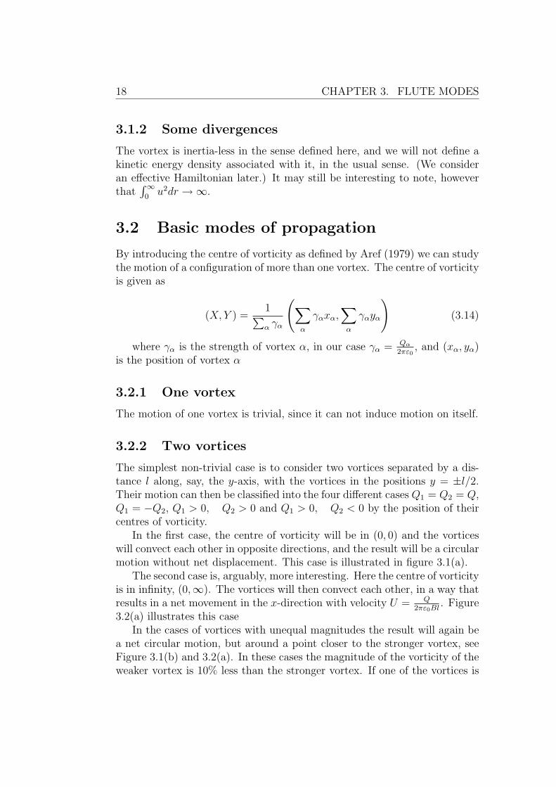
The second case is, arguably, more interesting. Here the centre of vorticityis in infinity, (0,∞). The vortices will then convect each other, in a way thatresults in a net movement in the x-direction with velocity U = Q
2πε0Bl. Figure
3.2(a) illustrates this caseIn the cases of vortices with unequal magnitudes the result will again be
a net circular motion, but around a point closer to the stronger vortex, seeFigure 3.1(b) and 3.2(a). In these cases the magnitude of the vorticity of theweaker vortex is 10% less than the stronger vortex. If one of the vortices is
3.2. BASIC MODES OF PROPAGATION 19
0 0.2 0.4 0.6 0.8 1−0.5
0
0.5
x(λD)
y(λ
D)
(a) (b)
Figure 3.1: The trajectory followed by two vortices of equal sign. (a) showsthe trajectories when both vortices have the same strength Q = 1 while (b)shows the trajectories when Q1 = 1.0 and Q2 = 0.9
much stronger than the other the result will be that the weaker orbits thestronger, with the stronger almost stationary.
3.2.3 Collision of two vortex pairs
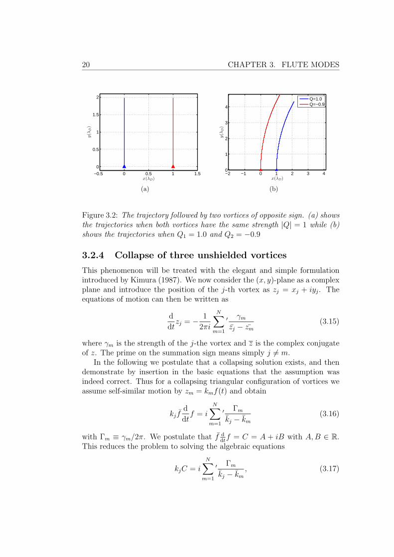
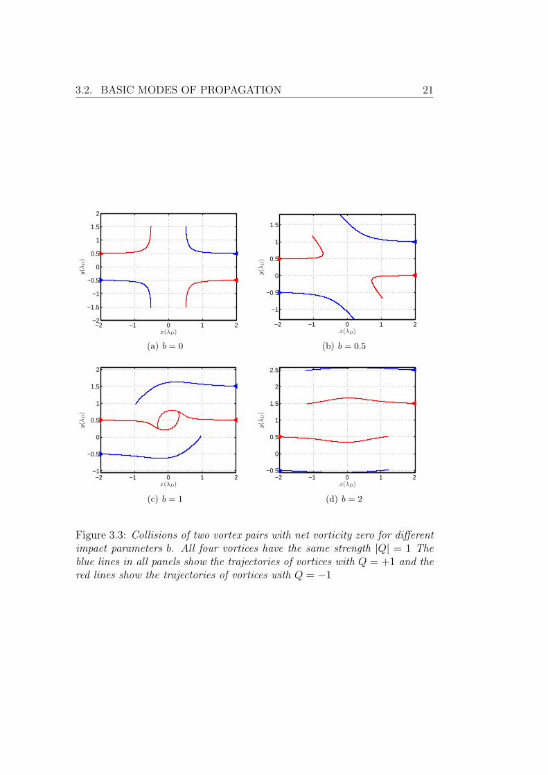
If we arrange four vortices as shown by the arrowheads in Figure 3.3(a), withthe blue arrowheads representing the vortices with positive polarities andthe red representing the negative, the resulting motion of the four vorticesare shown by the trajectories in Figure 3.3(a). This shows a collision oftwo vortex pairs; the pairs will independently move as described above whenthe separation between the pairs are larger than the distance between thevortices, the pairs then interact and change partners and directions.
If we shift one of the pairs a distance b in the y-direction, we call thisdistance the impact parameter and the case above is b = 0, we get differentbehaviour. The trajectories for different values of b is shown in figure 3.3.For low b the result is an elastic collision where the vortices change partnersand direction; when b is almost equal to the distance between the vortices,the result is what could be called an inelastic collision, where the two vorticeswith the same polarity meet and move a circular trajectory with the othertwo vortices orbiting. When b is twice the separation, as shown in Figure3.3(d) the pairs pass without much interaction and for increasing b the resultapproaches two independently propagating vortex pairs.
20 CHAPTER 3. FLUTE MODES
−0.5 0 0.5 1 1.5
0
0.5
1
1.5
2
x(λD)
y(λ
D)
(a)
−2 −1 0 1 2 3 40
1
2
3
4
x(λD)
y(λ
D)
Q=1.0Q=−0.9
(b)
Figure 3.2: The trajectory followed by two vortices of opposite sign. (a) showsthe trajectories when both vortices have the same strength |Q| = 1 while (b)shows the trajectories when Q1 = 1.0 and Q2 = −0.9
3.2.4 Collapse of three unshielded vortices
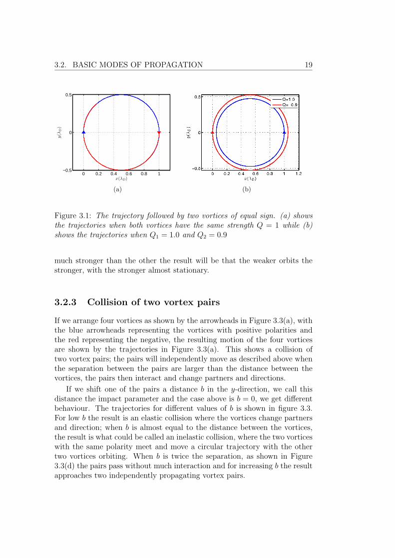
This phenomenon will be treated with the elegant and simple formulationintroduced by Kimura (1987). We now consider the (x, y)-plane as a complexplane and introduce the position of the j-th vortex as zj = xj + iyj. Theequations of motion can then be written as
d
dtzj = − 1
2πi
N∑m=1
′ γmzj − zm
(3.15)
where γm is the strength of the j-the vortex and z is the complex conjugateof z. The prime on the summation sign means simply j 6= m.
In the following we postulate that a collapsing solution exists, and thendemonstrate by insertion in the basic equations that the assumption wasindeed correct. Thus for a collapsing triangular configuration of vortices weassume self-similar motion by zm = kmf(t) and obtain
kj fd
dtf = i
N∑m=1
′ Γmkj − km
(3.16)
with Γm ≡ γm/2π. We postulate that f ddtf = C = A + iB with A,B ∈ R.
This reduces the problem to solving the algebraic equations
kjC = iN∑m=1
′ Γmkj − km
, (3.17)
3.2. BASIC MODES OF PROPAGATION 21
−2 −1 0 1 2−2
−1.5
−1
−0.5
0
0.5
1
1.5
2
x(λD)
y(λ
D)
(a) b = 0
−2 −1 0 1 2
−1
−0.5
0
0.5
1
1.5
x(λD)
y(λ
D)
(b) b = 0.5
−2 −1 0 1 2−1
−0.5
0
0.5
1
1.5
2
x(λD)
y(λ
D)
(c) b = 1
−2 −1 0 1 2−0.5
0
0.5
1
1.5
2
2.5
x(λD)
y(λ
D)
(d) b = 2
Figure 3.3: Collisions of two vortex pairs with net vorticity zero for differentimpact parameters b. All four vortices have the same strength |Q| = 1 Theblue lines in all panels show the trajectories of vortices with Q = +1 and thered lines show the trajectories of vortices with Q = −1
22 CHAPTER 3. FLUTE MODES
−0.8 −0.6 −0.4 −0.2 0 0.2 0.4 0.6 0.8
−0.4
−0.2
0
0.2
0.4
0.6
0.8
x(λD)
y(λ
D)
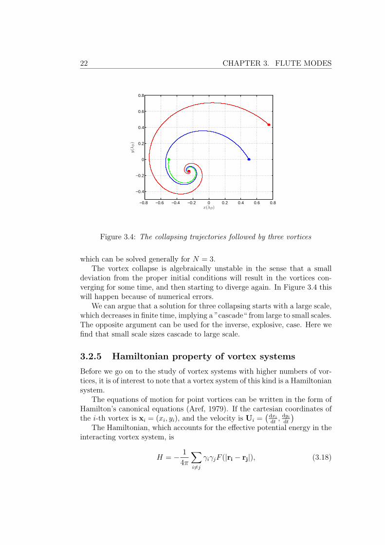
Figure 3.4: The collapsing trajectories followed by three vortices
which can be solved generally for N = 3.The vortex collapse is algebraically unstable in the sense that a small
deviation from the proper initial conditions will result in the vortices con-verging for some time, and then starting to diverge again. In Figure 3.4 thiswill happen because of numerical errors.
We can argue that a solution for three collapsing starts with a large scale,which decreases in finite time, implying a ”cascade“ from large to small scales.The opposite argument can be used for the inverse, explosive, case. Here wefind that small scale sizes cascade to large scale.
3.2.5 Hamiltonian property of vortex systems
Before we go on to the study of vortex systems with higher numbers of vor-tices, it is of interest to note that a vortex system of this kind is a Hamiltoniansystem.
The equations of motion for point vortices can be written in the form ofHamilton’s canonical equations (Aref, 1979). If the cartesian coordinates ofthe i-th vortex is xi = (xi, yi), and the velocity is Ui =
(dxidt, dyi
dt
)The Hamiltonian, which accounts for the effective potential energy in the
interacting vortex system, is
H = − 1
4π
∑i 6=j
γiγjF (|ri − rj|), (3.18)
3.2. BASIC MODES OF PROPAGATION 23
where F (|r|) is some function accounting for the interaction between vor-tices and γi is the strength of vortex i. In the case of unshielded vorticesF (|r|) = ln(|r|) and for the shielded vortices described in section 3.1.1,F (|r|) = K0(κ|r|), but F can in fact be of a broad class of interactions,some of which might not be physically realizable (Lynov et al., 1991). Theymight, however, have the advantage of removing the singularity at r = 0 inthe simple vortices used here.
By using the expression for the Hamiltonian (3.18) and the expression forvelocity we can see that
γidxidt
=∂H
∂yi(3.19)
γidyidt
= −∂H∂xi
, (3.20)
which is on the same form as Hamilton’s equations
dpidt
= −∂H∂qi
,dqidt
=∂H
∂pi, (3.21)
with xi taking the role of generalised coordinate and yi taking the role ofgeneralised momentum. This means, as far as the hamiltonian is concerned,that one spatial coordinate is a “coordinate” and the other is a generalisedmomentum. This system does not contain any kinetic energy in the usualsense, since the vortices move like massless particles, instantly assuming thelocal flow velocity. Expression 3.18 for the Hamiltonian only applies forunbounded systems. The presence of periodic boundary conditions breakrotational symmetry, and the potential will have to be modified.
Since the Hamiltonian does not depend explicitly on time, it is an integralof motion. The Hamiltonian is, as well, invariant to translations and rotationsof the coordinates, this implies three conservation laws.
∑i
γixi = constant (3.22)∑i
γiyi = constant (3.23)∑i
γi(x2i + y2
i ) = constant. (3.24)
If the sum of all vortex strengths is non-zero,∑
i γi 6= 0, the centre ofvorticity is a fixed point for the flow with coordinates
X, Y ≡ 1∑i γi
∑i
γixi,∑i
γiyi
. (3.25)
24 CHAPTER 3. FLUTE MODES
By introducing the vortex separation as li,j ≡ |ri − rj|, it can be shown that
1
2
∑i
γiγjl2i,j =
(∑i
γi
)∑j
γj(x2j + y2
j )
−
(∑i
γixi
)2
−
(∑i
γixi
)2
, (3.26)
is a constant of motion as well, independent of the reference system. Fromequations (3.19) it is possible to derive an expression for the square of thevortex separation without reference to the absolute positions of the vortices.For unshielded vortices we have
d
dtl2i,j =
2
π
∑k 6=i,k 6=j
γkσi,j,kAi,j,k
(1
l2j,k− 1
l2k,i
), (3.27)
where the sum excludes k = i and k = j. The quantity σi,j,k defines theorientation of the triangle spanned by three vortices i, j, k so that σi,j,k = +1if i, j, k appear in counter clockwise order, and σi,j,k = −1 otherwise. Ai,j,kis the area of the triangle. Note that σi,j,k is undefined if the three vorticesare on a line, but that in this case the area is zero.
The relations (3.25) together with the Hamiltonian (3.18) and the con-stant of motion (3.26) defines the problem of the motion of N vortices. Equa-tion (3.25) indicates that the problem of N = 3 is fundamental for the under-standing of N > 3, since 3 is the lowest number of vortices where the righthand side of (3.25) is nonzero, and the separation of the vortices is not aconstant of motion. This means that if we consider the separations as quan-titative measures of excited scales of motion, the three-vortex interaction isthe lowest order interaction capable of exciting new scales. The three vortexproblem is Hamiltonian with six degrees of freedom and four constants ofmotion with the vortex strengths as constant parameters, and as such is in-tegrable as shown by Poincare (1893) (See Aref (1983) for a historical reviewof the research on vortex dynamics.). Some of the solutions of this motion ishighly unexpected and surprising, so a summary of these special results willbe given before embarking on the treatment of N vortices.
3.3 Many vortices
3.3.1 Many vortices with deterministic positions
For cases with more than two vortices, it is possible to construct stablepatterns of vortices. See for example (Morikawa and Swenson, 1971) for a
3.3. MANY VORTICES 25
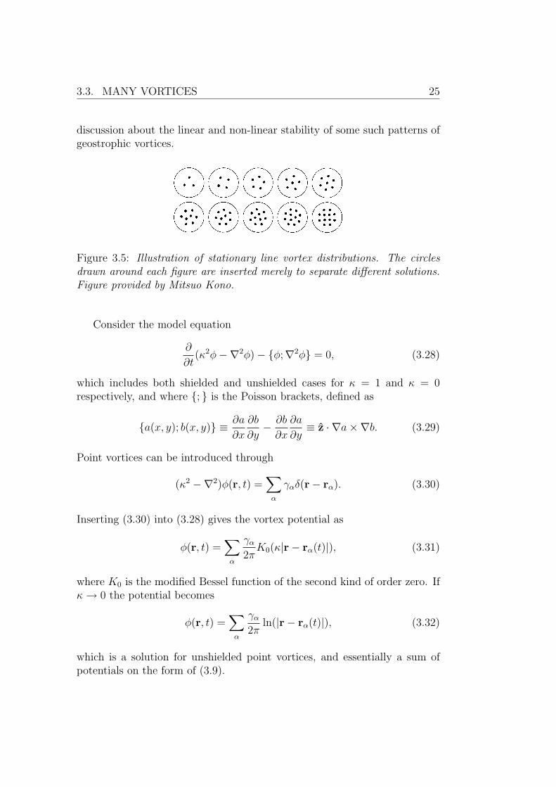
discussion about the linear and non-linear stability of some such patterns ofgeostrophic vortices.
Figure 3.5: Illustration of stationary line vortex distributions. The circlesdrawn around each figure are inserted merely to separate different solutions.Figure provided by Mitsuo Kono.
Consider the model equation
∂
∂t(κ2φ−∇2φ)− φ;∇2φ = 0, (3.28)
which includes both shielded and unshielded cases for κ = 1 and κ = 0respectively, and where ; is the Poisson brackets, defined as
a(x, y); b(x, y) ≡ ∂a
∂x
∂b
∂y− ∂b
∂x
∂a
∂y≡ z · ∇a×∇b. (3.29)
Point vortices can be introduced through
(κ2 −∇2)φ(r, t) =∑α
γαδ(r− rα). (3.30)
Inserting (3.30) into (3.28) gives the vortex potential as
φ(r, t) =∑α
γα2πK0(κ|r− rα(t)|), (3.31)
where K0 is the modified Bessel function of the second kind of order zero. Ifκ→ 0 the potential becomes
φ(r, t) =∑α
γα2π
ln(|r− rα(t)|), (3.32)
which is a solution for unshielded point vortices, and essentially a sum ofpotentials on the form of (3.9).
26 CHAPTER 3. FLUTE MODES
The equations of motion for the vortices are
d
dtrα = z×∇φ(rα, t)
=κ
2π
∑β
γβz× (rα − rβ)
|rα − rβ|K1(κ|rα − rβ|), (3.33)
where the K1-function arises from the differentiation of K0. These equationsmean, physically, that each vortex, at any time, is convected by the superim-posed velocity field from all the other vortices. When the distances betweenvortices is short enough, compared to the shielding distance, shielding canbe neglected, and the equation (3.34) simplifies to
d
dtrα =
1
2π
∑β
γβz× (rα − rβ)
|rα − rβ|2(3.34)
for κ→ 0, which could also have been derived from equation (3.32)Equilibrium configurations have been discussed by Morikawa and Swen-
son (1971) for N vortices equally distributed on a circle without a centrevortex, see e.g. Figure 3.5. They found that for 2 ≤ N ≤ 6 the configurationis stable for κ < 1.289 and that N = 7 is stable for κ = 0. When a centrevortex is present the configuration N = 3 is stable for κ ≥ 3.50, configura-tions of N = 4, 5, 6, 7 vortices are stable for all κ, for N = 8 the configurationis stable for κ < 1.597 and N = 9 gives a stable configuration only for κ = 0.
A more general analysis Kono et al. (1998) can be made by introducingthe distribution function
f(r, t) =∑α
γαδ(r− rα(t)) (3.35)
and rewriting equation 3.34 as
∂
∂tf(r, t) = − κ
2π
∫dr′
K1(κ|r− r′|)|r− r′|
z× (r− r′) · ∇f(r′, t)f(r, t) (3.36)
Changing coordinates from Cartesian to cylindrical (r, θ) and rememberingthat
z× (r− r′) · ∇ = −r′ sin(θ − θ′) ∂∂r
+
[1− r′
rcos(θ − θ′)
]∂
∂θ, (3.37)
we get
∂
∂tf(r, θ, t) + Ω(r, θ, t)
∂
∂θf(r, θ, t) + V (r, θ, t)
∂
∂rf(r, θ, t) = 0, (3.38)
3.3. MANY VORTICES 27
where
Ω(r, θ, t) = − κ
2π
∫dr′
K1(κ|r− r′|)|r− r′|
[1− r′
rcos(θ − θ′)
]f(r, θ, t) (3.39)
V (r, θ, t) = − κ
2π
∫dr′r′
K1(κ|r− r′|)|r− r′|
sin(θ − θ′)f(r, θ, t) (3.40)
From equations (3.39) and (3.40) equilibrium configurations are obtained byimposing that V (r, θ, t) has to be identically zero and that Ω(r, θ, t) has tobe constant. Under these conditions the system is rigidly rotating aroundthe origin without any radial displacement
It is, using the foregoing equations, possible to look for stable concentricstructures of M rings with radius am with Nm identical vortices equallydistributed on the m-th ring (m = 1, ...,M). This means that γα = γ.The pattern can be with or without a center vortex γ0 which corresponds toγ0 = γ or γ0 = 0. Then
f(r, θ, t) =∑m,n
γ
amδ(r − am)δ(θ − θm,n) +
γ0
rδ(r)δ(θ) (3.41)
for which the following holds in equilibriun
V (m0, n0) = −κ2
2πγ∑m,n
amσm,n
K1(σm,n) sin(θm0,n0 − θm,n) = 0 (3.42)
and
Ω(m0, n0) = −κ2
2πγ∑m,n
1
σm,nK1(σm,n)
[1− am
am0
cos(θm0,n0 − θm,n)
]+
κ
2πγ0K1(κam0)
am0
= const, (3.43)
where
σm,n = κ√a2m0
+ a2m − 2am0am cos(θm0,n0 − θm, n) (3.44)
and (m,n) refers to the n-th vortex on the m-th ring and (m0, n0) refers tothe coordinates of an arbitrary reference vortex.
If the vortices are distributed on each circle, in such a way that that thedistances between neighbouring vortices is the same, as illustrated in Figure3.5, that is θm,n = 2πn/Nm where Nm is the number of vortices on the m-thcircle, then V (m0, n0) is always equal to zero and Ω(m0, n0) does not dependon n0 because of symmetry.
28 CHAPTER 3. FLUTE MODES
3.4 Randomly distributed ensemble of vor-
tices
3.4.1 Localised cloud
The dynamics of a localised cloud will depend on the sign of the vorticities.If all vortices have the same polarity, the dominating motion will be on ofrotation, since the total vorticity is large. The Hamiltonian of this systemwill be large and positive. The cloud will rotate almost as a rigid body andwe expect that the cloud will preserve it’s identity and structure over time.
A cloud with approximately zero total vorticity will have no net rotation,and we will expect that vortices with opposite polarities will pair up andpropagate away from the cloud. This system will have a small Hamiltoniansince pairs of ++,+−,−+,−− have equal probability. We do not expectthis system to preserve it’s structure over time.
3.4.2 Homogeneous ensembles
With an infinite system, we mean one which is homogeneous, isotropic andin equilibrium, so, apart form random fluctuations, the quantities are timestationary. The transport properties of such an infinite system will be treatedas those arising from a random turbulent velocity field, and discussed in detailin Chapter 4.
The realisation of such a system for numerical simulation is treated inChapter 5.
3.5 Negative temperatures
In standard applications of classical statistical mechanics the idea of negativetemperatures might seem to be leading to paradoxes. It might be worthwhileto give a simple illustrative summary demonstrating the properties of realiz-able physical systems which can logically be assigned a negative temperature(Marvan, 1966). Such systems consisting of simple particle spins are to someextent simpler to analyse than a collection of line vortices.
Standard and intuitive objections to the concept of negative temperaturesare often based on models derived from ideal gases, and indeed it will notbe possible to give a meaningful definition of negative temperatures in thatcontext. We heat a gas by supplying energy: the more energy we add,the warmer the gas becomes. On the other hand we will not be able tocool the gas below the absolute zero. Note, however, that although energy
3.5. NEGATIVE TEMPERATURES 29
a)
b)
c)
d)
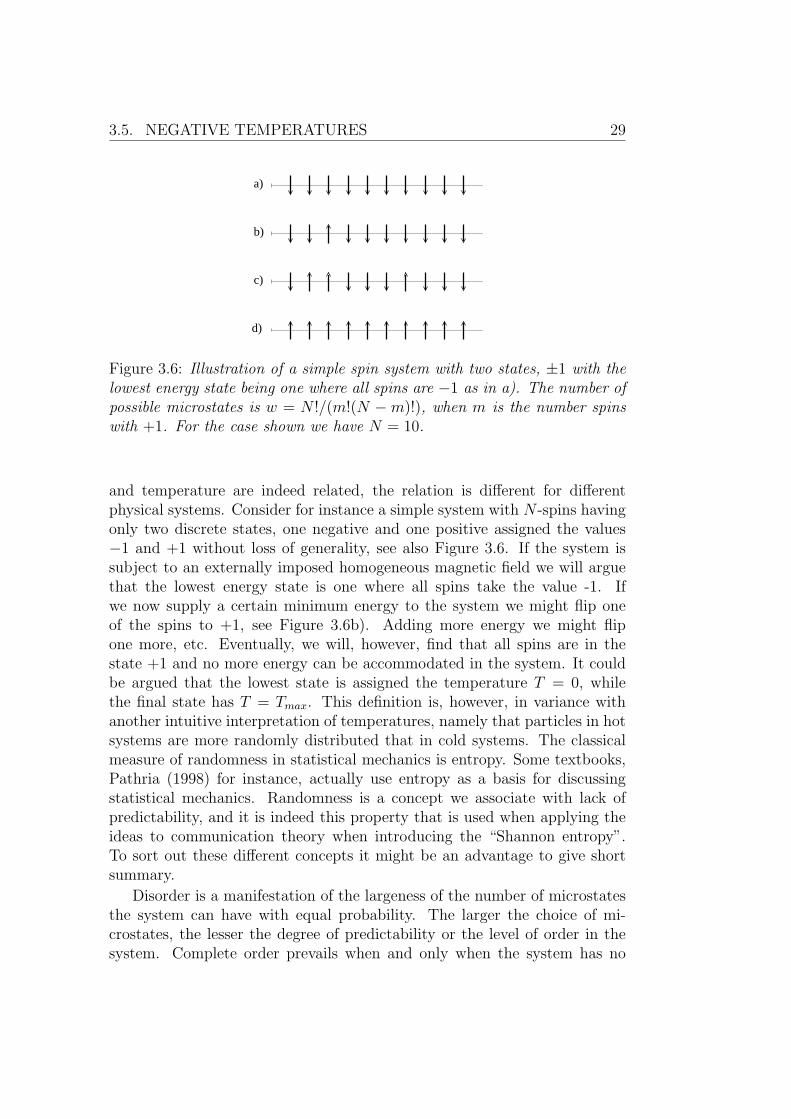
Figure 3.6: Illustration of a simple spin system with two states, ±1 with thelowest energy state being one where all spins are −1 as in a). The number ofpossible microstates is w = N !/(m!(N −m)!), when m is the number spinswith +1. For the case shown we have N = 10.
and temperature are indeed related, the relation is different for differentphysical systems. Consider for instance a simple system with N -spins havingonly two discrete states, one negative and one positive assigned the values−1 and +1 without loss of generality, see also Figure 3.6. If the system issubject to an externally imposed homogeneous magnetic field we will arguethat the lowest energy state is one where all spins take the value -1. Ifwe now supply a certain minimum energy to the system we might flip oneof the spins to +1, see Figure 3.6b). Adding more energy we might flipone more, etc. Eventually, we will, however, find that all spins are in thestate +1 and no more energy can be accommodated in the system. It couldbe argued that the lowest state is assigned the temperature T = 0, whilethe final state has T = Tmax. This definition is, however, in variance withanother intuitive interpretation of temperatures, namely that particles in hotsystems are more randomly distributed that in cold systems. The classicalmeasure of randomness in statistical mechanics is entropy. Some textbooks,Pathria (1998) for instance, actually use entropy as a basis for discussingstatistical mechanics. Randomness is a concept we associate with lack ofpredictability, and it is indeed this property that is used when applying theideas to communication theory when introducing the “Shannon entropy”.To sort out these different concepts it might be an advantage to give shortsummary.
Disorder is a manifestation of the largeness of the number of microstatesthe system can have with equal probability. The larger the choice of mi-crostates, the lesser the degree of predictability or the level of order in thesystem. Complete order prevails when and only when the system has no
30 CHAPTER 3. FLUTE MODES
5 10 15 20m
-10
-5
0
5
10
kT
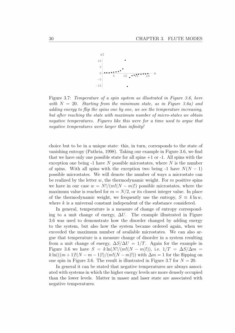
Figure 3.7: Temperature of a spin system as illustrated in Figure 3.6, herewith N = 20. Starting from the minimum state, as in Figure 3.6a) andadding energy to flip the spins one by one, we see the temperature increasing,but after reaching the state with maximum number of micro-states we obtainnegative temperatures. Figures like this were for a time used to argue thatnegative temperatures were larger than infinity!
choice but to be in a unique state: this, in turn, corresponds to the state ofvanishing entropy (Pathria, 1998). Taking our example in Figure 3.6, we findthat we have only one possible state for all spins +1 or -1. All spins with theexception one being -1 have N possible microstates, where N is the numberof spins. With all spins with the exception two being -1 have N(N − 1)possible microstates. We will denote the number of ways a microstate canbe realized by the letter w, the thermodynamic weight. For m positive spinswe have in our case w = N !/(m!(N −m)!) possible microstates, where themaximum value is reached for m = N/2, or its closest integer value. In placeof the thermodynamic weight, we frequently use the entropy, S ≡ k lnw,where k is a universal constant independent of the substance considered.
In general, temperature is a measure of change of entropy correspond-ing to a unit change of energy, ∆U . The example illustrated in Figure3.6 was used to demonstrate how the disorder changed by adding energyto the system, but also how the system became ordered again, when weexceeded the maximum number of available microstates. We can also ar-gue that temperature is a measure change of disorder in a system resultingfrom a unit change of energy, ∆S/∆U = 1/T . Again for the example inFigure 3.6 we have S = k ln(N !/(m!(N − m)!)), i.e. 1/T = ∆S/∆m =k ln(((m+ 1)!(N −m− 1)!)/(m!(N −m)!)) with ∆m = 1 for the flipping onone spin in Figure 3.6. The result is illustrated in Figure 3.7 for N = 20.
In general it can be stated that negative temperatures are always associ-ated with systems in which the higher energy levels are more densely occupiedthan the lower levels. Matter in maser and laser state are associated withnegative temperatures.
3.5. NEGATIVE TEMPERATURES 31
3.5.1 Negative temperature states
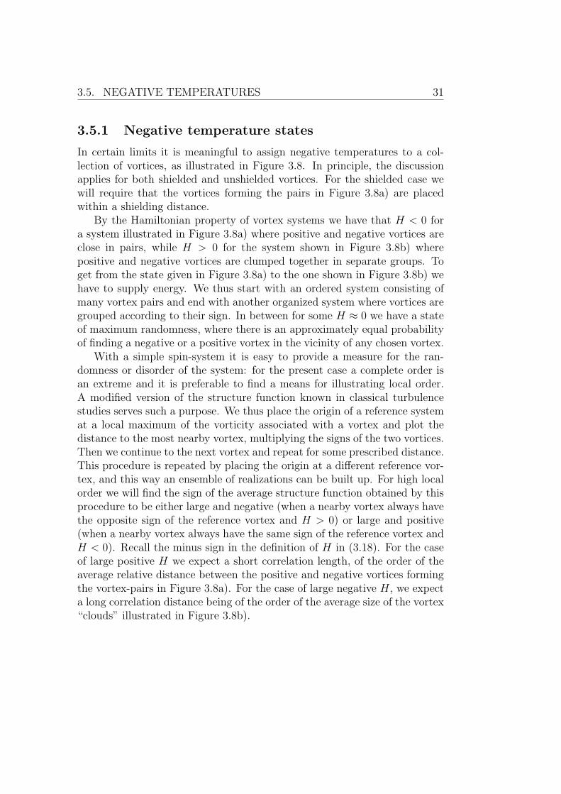
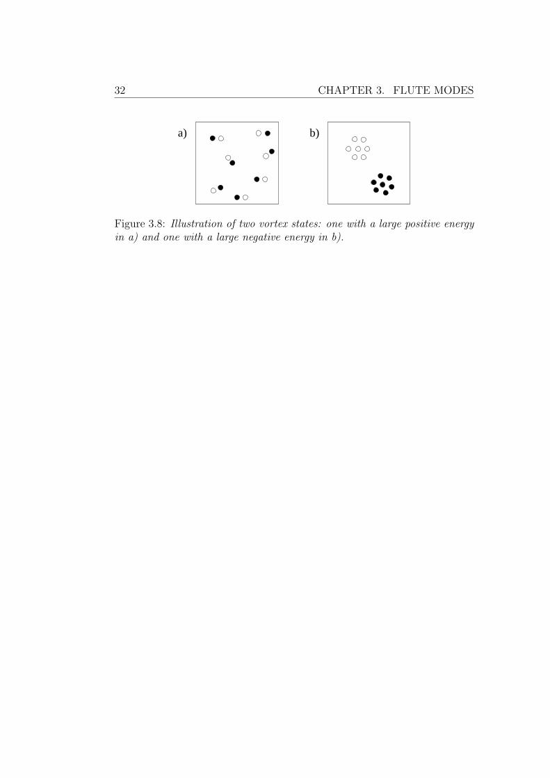
In certain limits it is meaningful to assign negative temperatures to a col-lection of vortices, as illustrated in Figure 3.8. In principle, the discussionapplies for both shielded and unshielded vortices. For the shielded case wewill require that the vortices forming the pairs in Figure 3.8a) are placedwithin a shielding distance.
By the Hamiltonian property of vortex systems we have that H < 0 fora system illustrated in Figure 3.8a) where positive and negative vortices areclose in pairs, while H > 0 for the system shown in Figure 3.8b) wherepositive and negative vortices are clumped together in separate groups. Toget from the state given in Figure 3.8a) to the one shown in Figure 3.8b) wehave to supply energy. We thus start with an ordered system consisting ofmany vortex pairs and end with another organized system where vortices aregrouped according to their sign. In between for some H ≈ 0 we have a stateof maximum randomness, where there is an approximately equal probabilityof finding a negative or a positive vortex in the vicinity of any chosen vortex.
With a simple spin-system it is easy to provide a measure for the ran-domness or disorder of the system: for the present case a complete order isan extreme and it is preferable to find a means for illustrating local order.A modified version of the structure function known in classical turbulencestudies serves such a purpose. We thus place the origin of a reference systemat a local maximum of the vorticity associated with a vortex and plot thedistance to the most nearby vortex, multiplying the signs of the two vortices.Then we continue to the next vortex and repeat for some prescribed distance.This procedure is repeated by placing the origin at a different reference vor-tex, and this way an ensemble of realizations can be built up. For high localorder we will find the sign of the average structure function obtained by thisprocedure to be either large and negative (when a nearby vortex always havethe opposite sign of the reference vortex and H > 0) or large and positive(when a nearby vortex always have the same sign of the reference vortex andH < 0). Recall the minus sign in the definition of H in (3.18). For the caseof large positive H we expect a short correlation length, of the order of theaverage relative distance between the positive and negative vortices formingthe vortex-pairs in Figure 3.8a). For the case of large negative H, we expecta long correlation distance being of the order of the average size of the vortex“clouds” illustrated in Figure 3.8b).
32 CHAPTER 3. FLUTE MODES
a) b)
Figure 3.8: Illustration of two vortex states: one with a large positive energyin a) and one with a large negative energy in b).
Chapter 4
Turbulent diffusion andtransport
Diffusion is an important transport phenomenon in many physical systems.Classical diffusion can be derived from simple random walk processes andwill usually be slow. In many plasma physics systems, the transport is manytimes higher than this classical diffusion (Tennekes and Lumley, 1972). Thesesystems are often turbulent and one of the most important properties ofturbulent flows is their ability to disperse particles at a rate which by farexceeds transport by classical molecular diffusion (Tennekes and Lumley,1972). This property is the same for neutral fluids and for plasmas.
We will make some general remarks on classical diffusion and Brownianmotion, and we will present some basic results on turbulent diffusion.
4.1 Classical diffusion
Classical diffusion can be derived from the continuity equation (see section2.3.3 and (3.1), (3.2)) on the form
∂φ(r, t)
∂t+∇ · j = 0 (4.1)
where φ(r, t) is the density of the diffusing material at point r and time t, andj is the flux of the diffusing material. φ can represent any scalar quantity, alsotemperature. No material is created or destroyed. By postulating that thedriving force of the flux is a gradient in φ and that this force is proportionalto ∇φ, this is called Fick’s first law1, i.e. j = −D(φ)∇φ(r, t) we arrive at the
1This is a phenomenological law based on the experimentally confirmed assumptionthat macroscopic fluxes originate from density gradients (Rumer and Ryvkin, 1980).
33
34 CHAPTER 4. TURBULENT DIFFUSION AND TRANSPORT
diffusion equation.
∂φ(r, t)
∂t= ∇ · [D(φ)∇φ(r, t)] (4.2)
which simplifies to the linear diffusion equation if D(φ) = D = constant
∂φ
∂t= D∇2φ. (4.3)
4.1.1 Diffusion of a light particle
Consider a light point charge which is free to move due to collisions withother particles in the environment. The displacement of this particle canbe analysed quite simply (Pecseli, 2000). The particle will have constantvelocity w between collisions, so it’s displacement from z0 in the z-directionis z = z0 + wt until the next collision. The displacement relative to z0 canbe written on the form
z =
∫ t1
0
w1dt+
∫ t2
t1
w2dt+ ...+
∫ TtN1
wNdt =N∑r=1
wr(tr−1 − tr) (4.4)
and similarly for the other coordinates. We assume that the velocity of theparticle after each collision is random with 〈wr〉 = 0 and independent of thevelocity before the collision. Then 〈z〉 = 0 is trivial. To get a non-trivialresult we consider 〈z2〉
〈z2〉 =N∑s=1
n∑r=1
〈wswr(ts−1 − ts)(tr−1tr)〉. (4.5)
If we now consider a very short time interval T in which collisions can beignored, we get z =
∫ T0w1dt = w1T and
〈z2〉 = w21T 2 (4.6)
This short time limit is determined purely by inertial effects and is indepen-dent on collision frequency.
Now we consider the particle after it has undergone many collisions. Sincethe velocities in different time intervals are statistically independent and also
4.2. TURBULENT DIFFUSION 35
independent of the particular time interval, we get
〈z2〉 =N∑s=1
n∑r=1
〈wswr(ts−1 − ts)(tr−1tr)〉
= 〈w2〉N∑s=1
〈(ts−1 − ts)2〉
= 2κT
m
N
ν2,
where ν is the particle collision frequency. We assumed that 〈wswr〉 =〈w2
s〉δr,s = 〈w2〉δr,s in terms of the Kronecker delta, since the particle’s veloc-ity after the collision is considered completely uncorrelated to the velocitybefore the collision. (This assumption is valid for light particles, but not forheavy particles moving against a background of light particles.) We used〈(ts−1 − ts)2〉 = 1/ν2 for all s. With the assumption that the particle beingin thermal equilibrium after one collision, we also used 〈w2〉 = κT/m. Thenumber of collisions, N , in the series varies statistically from realization torealization and, averaging over the realizations, we have 〈N〉 = T ν. Thisgives
〈z2〉 = 2κT
m
Tν. (4.7)
This limit for large T is often called the diffusion limit with referenceto the solutions of the standard diffusion equation; see Section 4.1. In thiscase the diffusing material would be the probability density P (z, t) for theparticles displacement z. The solution to this diffusion equation is P (z, t) =√
4πDt exp[−z2/(4Dt)] if the particle was at z = 0 at t = 0, i.e. P (z, t =0) = δ(z). In this case we get 〈z2〉 =
∫∞−∞ z
2P (t, z) = 2Dt which is analogousto (4.7) if we define
D =〈w2〉ν
=κT
mν. (4.8)
4.2 Turbulent diffusion
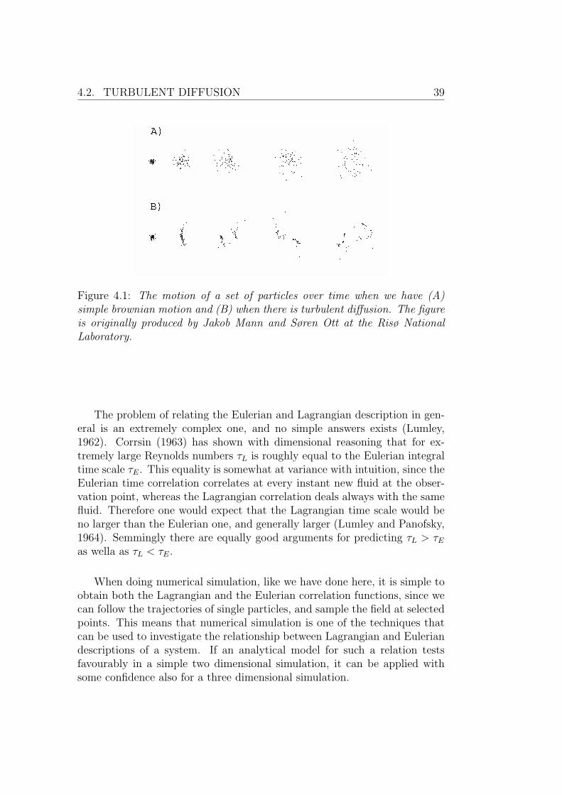
Turbulent diffusion is manifestly different form classical Brownian diffusion.This is best seen by considering a cloud of particles released at the sametime, see Figure 4.1. Turbulent diffusion moves and distorts the entire cloud,but in the asymptotic diffusion limit (t → ∞), the two figures (A) and (B)tends to become similar.
We will now show some of the basic results on turbulent diffusion. Theoutline is independent of the dimensionality of the problem and the ideas
36 CHAPTER 4. TURBULENT DIFFUSION AND TRANSPORT
apply equally well for three dimensional and two dimensional turbulence,given the assumption of homogeneity and isotropy. Particle displacement willbe expressed in terms of a velocity, but this velocity can be obtained froman electrostatic electric field in magnetized plasmas as u(r, t) = E(r, t) ×B0/B
20 for homogeneous magnetic fields, assuming low frequency turbulence
where all relevant frequencies are ω Ωci. This model will then assumetwo dimensional turbulence in the plane ⊥ B0. Many experiments havedemonstrated that turbulent transport is an important mechanism in forinstance fusion plasma experiments (Liewer, 1985), and significant effortshave been made to understand this mechanism for anomalous transport alsoin the context of drift wave turbulence (Horton, 1999).
4.2.1 Single particle diffusion
Let us again consider the simplest possible problem, namely the one where asingle particle is released in a homogeneous and isotropic turbulent velocityfield, u(r, t); the field generated from an ensemble of vortices is such a velocityfield. We assume that the particle is convected as a passive scalar by theflow, and want to determine its mean-square displacement with respect tothe origin of release, which we without loss of generality take to be at theorigin of the coordinate system (Roberts, 1957).
Since, by assumption, dr(t)/dt = u(r(t), t), we have in a given realizationof the flow the particle position to be
r(t) =
∫ t
0
u(r(t′), t′)dt′ . (4.9)
The average position 〈r(t)〉 vanishes, since we have assumed 〈u(r(t), t)〉 = 0.This is actually not quite as self evident as it might appear (Tennekes andLumley, 1972), since we can assume from the outset only that 〈u(r, t)〉 = 0,but this is concerning a function of a spatial as well as a temporal variable,while 〈u(r(t), t)〉 is a function of time alone. We postpone the discussion ofthis question.
The mean square displacement is a positive quantity, and we find
r(t) · dr(t)
dt=
1
2
dr2(t)
dt= u(r(t), t) ·
∫ t
0
u(r(t′), t′)dt′
=
∫ t
0
u(r(t), t) · u(r(t′), t′)dt′ . (4.10)
Taking the ensemble average, we have
d
dt
⟨r2(t)
⟩= 2
∫ t
0
〈u(r(t), t) · u(r(t′), t′)〉 dt′ . (4.11)
4.2. TURBULENT DIFFUSION 37
For time stationary turbulence we require 〈u(r(t), t) · u(r(t′), t′)〉 = RL(t −t′)〈u2〉, with the subscript L reminding us to sample the velocity field along aLagrangian orbit. We introduced RL as the normalized Lagrangian velocitycorrelation function, RL(0) = 1.
When integrating (4.10) as 〈r2(t)〉 = 2〈u2〉∫ t
0
∫ t′′0RL(t′′ − t′)dt′dt′′, it is
an advantage to introduce the variables τ ≡ t′′ − t′ and s ≡ t′′, giving theJacobian
J =
∂τ
∂t′′∂τ
∂t′
∂s
∂t′′∂s
∂t′
=1 -11 0
= 1 ,
so that dt′′dt′ = dτds. Making the variable transforms as indicated, wenote that we can change the order of integration as
∫ t0
∫ s0RL(τ)dτds =∫ t
0
∫ tτRL(τ)dsdτ to give
⟨r2(t)
⟩= 2t〈u2〉
∫ t
0
(1− τ/t)RL(τ)dτ . (4.12)
Two relevant limiting cases of (4.12) can be distinguished here (Roberts,1957).
1. Very short times, where it can be assumed that RL(τ) ≈ 1. In thislimit we find 〈r2(t)〉 ≈ 〈u2〉t2, which is often called the ballistic limitsince it is the result we would have obtained by assuming the particleto follow straight lines of orbit, r(t) = ut, and simply average over allvelocities. We might experience to find auto-correlation functions thatare not differentiable for τ = 0, and in such cases the ballistic limit doesnot exist. Such a case requires that 〈(du/dt)2〉 diverges. With finiteparticle inertia we would expect that du/dt should be finite at all times.The absence of a ballistic limit simply indicates a very rapidly changingvelocity field, and the interval where RL(τ) ≈ 1 may be negligible.
2. Very large times, t→∞, where it can be assumed that∫ t
0RL(τ)dτ ≈
τL, introducing the Lagrangian integral correlation time
τL ≡∫ ∞
0
RL(τ)dτ . (4.13)
In this limit we find the important result⟨r2(t)
⟩≈ 2tτL〈u2〉 . (4.14)
38 CHAPTER 4. TURBULENT DIFFUSION AND TRANSPORT
At least formally this looks like the result one obtains by using the clas-sical diffusion equation with a diffusion coefficient D ≡ 2τL〈u2〉 to ob-tain the mean square particle displacement. Such cases have 〈r2(t)〉 ∼ t.The limit of times much larger than the Lagrangian correlation time isconsequently called the diffusion limit. This limiting case is consistentwith a random walk with a typical length step τL
√〈u2〉 per time τL.
Note that r(t) is not a time-stationary random process, although it isderived from u(r, t) which can be assumed to be so! The initial time (thetime of release of the particle) has a special role for r(t).
Introducing the Lagrangian power spectrum,
SL(ω) ≡ (1/2π)
∫ ∞−∞
RL(t)e−iωtdt
, with RL(t) =∫∞−∞ SL(ω)eiωtdω, we can write the result (4.12) on the form
(Lumley and Panofsky, 1964)⟨r2(t)
⟩= t2 〈u2〉
∫ ∞−∞
(sin(ωt/2)
ωt/2
)2
SL(ω)dω . (4.15)
The function sin2(ωt/2)/(ωt/2)2 originates from the Fourier transform of the“triangular” function 1−τ/t entering the convolution (4.12). For large timesit is evident that dispersion of the test particle is primarily due to the lowfrequencies in the Lagrangian spectrum. We have limt→∞ sin(ωt/2)/(ω/2) =πδ(ω), so we recover τL = SL(ω = 0). Note that oscillations in the La-grangian spectrum with frequencies being multipla of 1/t do not contributeto the particle displacement. This is because they return the particle to itsstarting point after a time t (Batchelor, 1949). Often it is assumed thatlow frequencies in (4.15) corresponds to large wavelengths (or rather largescales), but we should be aware that there is no a priori reason to believethis.
By (4.15) our problem seems to be solved once and for all, at least forthe case of homogeneous isotropic turbulence! Alas, it is not so, since wedo not know the spectrum SL(ω), and it is very complicated to obtain itexperimentally. It has been a major enterprise over the years to find waysof predicting SL(ω) on the basis of the more readily measurable Euleriancorrelation function. Amazingly good results can be obtained, at least as faras predictions of 〈r2(t)〉 are concerned. However, this might as well implythat this is a very robust results, and that almost any reasonable guess onRL will give acceptable results. After all, we must require that RL(0) = 1and that RL(t → ∞) → 0, and with a little common sense all reasonableguesses of RL tend to look more or less the same.
4.2. TURBULENT DIFFUSION 39
Figure 4.1: The motion of a set of particles over time when we have (A)simple brownian motion and (B) when there is turbulent diffusion. The figureis originally produced by Jakob Mann and Søren Ott at the Risø NationalLaboratory.
The problem of relating the Eulerian and Lagrangian description in gen-eral is an extremely complex one, and no simple answers exists (Lumley,1962). Corrsin (1963) has shown with dimensional reasoning that for ex-tremely large Reynolds numbers τL is roughly equal to the Eulerian integraltime scale τE. This equality is somewhat at variance with intuition, since theEulerian time correlation correlates at every instant new fluid at the obser-vation point, whereas the Lagrangian correlation deals always with the samefluid. Therefore one would expect that the Lagrangian time scale would beno larger than the Eulerian one, and generally larger (Lumley and Panofsky,1964). Semmingly there are equally good arguments for predicting τL > τEas wella as τL < τE.
When doing numerical simulation, like we have done here, it is simple toobtain both the Lagrangian and the Eulerian correlation functions, since wecan follow the trajectories of single particles, and sample the field at selectedpoints. This means that numerical simulation is one of the techniques thatcan be used to investigate the relationship between Lagrangian and Euleriandescriptions of a system. If an analytical model for such a relation testsfavourably in a simple two dimensional simulation, it can be applied withsome confidence also for a three dimensional simulation.
40 CHAPTER 4. TURBULENT DIFFUSION AND TRANSPORT
4.2.2 Eulerian and Lagrangian mean-square velocities
Before closing the present discussion, we should clear up an ambiguity hintedalready: we introduced 〈u2〉 in a Lagrangian context: we should in principledistinguish ensemble averages of Eulerian and a Lagrangian velocities. Thesetwo are however simply related in cases relevant here. Consider first the Eu-lerian characteristic function for the fluctuating velocity which we can defineas the ensemble average 〈exp(ik · uE(r, t)〉. The corresponding structurefunction for the Lagrangian velocity field, as sampled by a self consistentlymoving passive test particle is 〈exp(ik · uL(r(t), t)〉. We then integrate thetwo exponential functions entering the characteristic functions over a (large)volume, V . Selecting a certain reference time, the volume is defined by thesame boundaries for both integrals, i.e. we have
1
V
∫V
exp(ik · uE(r, t))dr =1
V
∫V
exp(ik · uL(r(t), t))dr (4.16)
We now take the ensemble average of both sides of this relation, but inorder to have an expression involving the characteristic function, we wouldlike to move the average signs inside the integral signs. As far as the Eulerianintegral is concerned, we can retain the integration volume to be the same,without further ado, provided the flow is incompressible, as we have assumedfrom the outset here. Lagrangian integral is problematic, however. Here, thevolume is deformed as the flow defining the volume evolves. The relative de-formation is however, immaterial in the limit where V →∞, simply becausethe number of particles leaving the reference volume scales with the surfaceof V (Tennekes and Lumley, 1972). Consequently, we can formally considerthe surface of this volume as fixed also for the Lagrangian case. In the limitV →∞ we therefore have
limV→∞
1
V
⟨∫V
exp(ik ·UE(r, t))dr
⟩=
limV→∞
1
V
∫V
〈exp(ik · uE(r, t))〉dr =
limV→∞
1
V
⟨∫V
exp(ik · uL(r(t), t))dr
⟩=
limV→∞
1
V
∫V
〈exp(ik · uL(r(t), t))〉dr (4.17)
For homogeneous and isotropic turbulence we have 〈exp(ik · uE(r, t)〉 aswell as 〈exp(ik · uL(r(t), t)〉 being independent of position (that is the wholeidea with homogeneity and isotropy) and we can take these quantities outside
4.2. TURBULENT DIFFUSION 41
the integration. The integrations are then trivially giving the volume, whichcancels with the volume in the divisor and we and up with the relation
〈exp(ik · uE(r, t))〉 = 〈exp(ik · uL(r(t), t))〉 . (4.18)
When the characteristic functions for the Eulerian and the Lagrangian ve-locities are equal, we trivially have 〈u2
E〉 = 〈u2L〉 and we did right in avoiding
any subscript in (4.12). This is, however, correct only for homogeneous andisotropic incompressible turbulence. It is essential for the argument that theintegration volume is a known constant in (4.16) and (4.17). This is the casebecause the plasma is assumed to be incompressible, i.e. the plasma fills thesame area at all times in our two dimensonal model.
The velocity field mediating the turbulent transport is for absolute dif-fusion a stationary random process. The particle displacement is of coursesteadily increasing in a mean square sense, and is therefore not a stationaryrandom process.

42 CHAPTER 4. TURBULENT DIFFUSION AND TRANSPORT
Chapter 5
Numerical Model
To study the implications of larger ensembles of vortices, especially the trans-port properties of a random ensemble, we have implemented the model de-scribed in chapter 3 in a C++ program. The source code is included inappendix A. This chapter describes the implementation and the routinesused to simulate the system.
5.1 Assumptions and approximations
The magnetic field B is assumed to be purely in the z direction and allvariation in the plasma is assumed to be in the plane perpendicular toz.
The magnetic field is assumed to be homogeneous in the plane perpen-dicular to z.
The fields are electrostatic, and the plasma currents are not strongenough to perturb the magnetic field in the perpendicular direction.
The basic state of the plasma is homogeneous and isotropic. The vortexstructures are introduced as perturbations in the electrostatic potentialby introducing line charges.
All dynamics are assumed to occur on time-scales much longer than thecyclotron frequencies and on length scales much longer than the Larmorradius. This allows us to only consider the guiding centre motion andview the line charges as charged magnetic field lines.
To simulate the motion of electrostatic vortices, as described in section 3.1we will use a discretized version of the equations of motion for an ensemble of
43
44 CHAPTER 5. NUMERICAL MODEL
vortices; equation (3.33) with Debye shielding and equation (3.34) without.We will solve these equations numerically using the Runge-Kutta algorithmto the 4th order.
5.1.1 Dimensions
When representing numbers on a computer, we are limited by the maximumprecision, called double precision, allowed in most computer applications.When we work with numbers close to this limit, the errors in the representa-tion grows. This means that we will often like to express simulated system inunits which are typical for the physical system. This is done by dividing ourphysical quantity with a number with the same unit, and which is typical forthe system.
Two natural scales present themselves in this problem, the Debye length
λD =√
ε0T0
n0q20, and the E × B-velocity U0 = E0×B0
B20
where E0 = γ02πε0λD
. We
then retrieve a characteristic line charge density γ0 = q0/λD for two dimen-sional plasmas. Here subscript 0 refer to an arbitrary reference plasma. Byusing these natural scales, a natural time-scale t0 = λD
U0can be constructed.
By inserting the expressions for the Debye length and the E×B velocity weget
t0 =2πε2
0B0T0
e2n0γ0
.
All times will be expressed in this scale, which corresponds to the timeit takes for a particle moving with velocity U0 to travel one Debye length,given E0, B0, T0, n0 of an arbitrary plasma.
All quantities given in this, or later chapters, are, unless otherwise stated,normalized with the corresponding reference values.
5.2 Equations of motion
Since the vortices move like massless particles, their velocity is, at all times,the instantaneous E ×B-velocity generated by the ensemble of all vortices.The whole motion of one vortex in the field of all others is then described bythe equation
dr
dt= U, (5.1)
5.2. EQUATIONS OF MOTION 45
with the two component equations
ui =dxidt
In the x-direction (5.2)
vi =dyidt
In the y-direction (5.3)
where, as was described in section 3.1, the velocity U = (u, v) is the instan-taneous E×B-velocity, with direction E×B and magnitude E/B. E is theinstantaneous electric field from the vortex j 6= i evaluated in the positionof vortex i, and B = Bz, where z is the unit vector in the z direction, is thehomogeneous magnetic field in which the vortices are moving.
By insertion of the expression for the velocity in (5.2) and (5.3) the equa-tions of motion becomes
dxidt
=EyB
B2, (5.4)
dyidt
= −ExBB2
. (5.5)
5.2.1 Unshielded vortices
If the vortices are unshielded, the electrostatic potential of one vortex atposition r due to another in position rα is φ = γα ln(|r − rα|), as describedin section 3.1. This gives the electric field on one vortex in r from anotherin rα as
E = γαr− rα
(|r− rα|)2. (5.6)
5.2.2 Shielded vortices
If, on the other hand, the vortices are shielded, the potential of one vortexat position r due to another in position rα is modified to (equation (3.31))φ = γαK0(|r − rα|) where K0 is the modified Bessel function of the secondkind of order zero. This gives the electric field on one vortex in r from anotherin rα as
E = γαr− rα|r− rα|
K1(|r− rα|). (5.7)
Where K1 arises from the differentiation of K0 and is the modified Besselfunction of the second kind of order one.
46 CHAPTER 5. NUMERICAL MODEL
5.2.3 Modified Bessel functions
The modified Bessel functions of the second kind (sometimes known as mod-ified Bessel functions of the third kind) of order n for a real argument x canbe found from the recursion formula
Kn+1(x) = Kn−1(x) +2n
xKn(x), (5.8)
starting from K0(x) and K1(x). For the implementation of Debye shieldedvortex potentials we need to calculate K1(x). We calculate K1(x) from twodifferent polynomial approximations, one for 0 < x ≤ 2 (b1), which hastruncation error |ε < 8× 10⁻⁹|, and one for 2 ≤ x <∞ (b2) with truncationerror |ε| < 2.2×10⁻⁷. Using b1 requires the calculation of the modified Besselfunction of the first kind of order one I1 from it’s polynomial approximationvalid for −3.75 ≤ x ≤ 3.75 with truncation error |ε| < 8×10⁻⁹ (Abramowitzand Stegun, 1965: Handbook of Mathematical Functions).
All modified Bessel functions needed for this study were implementedin the routine called tbessk.cpp. This contains the functions necessary tocalculate Kn(x) and was originally written by Jean-Pierre Moreau1.
5.3 4th order Runge-Kutta algorithm
Integration of the equations of motion are performed with the 4th orderRunge-Kutta algorithm with variable time step, which, given an initial valueproblem
y = f(t, y), y(t0) = y0 (5.9)
is as follows:
yn+1 = yn +1
6(k1 + 2k2 + 2k3 + k4) (5.10)
tn+1 = tn + h (5.11)
where h is the iteration step length, yn+1 is the RK4 approximation of y(tn+1)and
k1 = hf(tn, yn) (5.12)
k2 = hf(tn +1
2h, yn +
1
2k1) (5.13)
k3 = hf(tn +1
2h, yn +
1
2k2) (5.14)
k4 = hf(tn + h, yn + k3) (5.15)
1Source:http://jean-pierre.moreau.pagesperso-orange.fr/c bessel.html
5.4. DISCRETIZED EQUATIONS OF MOTION 47
The next value (yn+1) is given by the previous value (yn) and the weightedaverage of four increments where each increment is the product of the steplength h and a slope estimated by the function f . From equations (5.12)-(5.15) we have
k1 is the increment based on the slope at the beginning of the intervalyn, and corresponds to Euler’s method
k2 is the increment based on the slope at the midpoint of the interval,using yn + 1
2k1
k3 is another increment based on the slope at the midpoint, but nowusing k2
k4 the increment using the slope at the end of the interval yn + k3
The weighted average is based on Simpson’s rule. RK4 is a fourth ordermethod, meaning that the stepwise error is on the order of h5 (O(h5)) andthe accumulated error is on the order of h4 (O(h4)).
Alternative integration schemes, like Euler’s method, Leapfrog and 2ndorder Runge-Kutta algorithm leads to accuracies O(h), O(h2) and O(h2)respectively. The Euler and Leapfrog methods are the fastest, both Runge-Kutta methods perform more calculations, and the Leapfrog method wouldbe preferred over 2nd order Runge-Kutta if 2nd order accuracy was sufficient.However for the vortex simulations carried out here the extra accuracy of theRK4 scheme is of sufficiently great value that the relative slowdown of thecode is an acceptable sacrifice.
5.4 Discretized equations of motion
Discretizing the equations of motion, (5.2) and (5.3), results in the set oftwo coupled equations for vortex i on the form of the RK4-algorithm givenabove:
xi,n+1 = xi,n +1
6(k1x + 2k2x + 2k3x + k4x) In the x-direction (5.16)
yi,n+1 = yi,n +1
6(k1y + 2k2y + 2k3y + k4y) In the y-direction. (5.17)
k1a, k2a, k3a, k4a in the a-direction are estimates of the position at t + ∆t asdescribed above. Given the initial conditions
xi(t = 0) = x0 (5.18)
yi(t = 0) = y0 (5.19)
48 CHAPTER 5. NUMERICAL MODEL
and estimates of the slopes
fxi(t, xi) = Ux =
∑j 6=iEy,jB
B2(5.20)
fyi(t, yi) = Uy = −∑
j 6=iEx,jB
B2(5.21)
where, again, Ey,j is the electric field from vortex j evaluated at the positionof vortex i. By this we have a closed system of discretized equations, whichcan be iterated to find the positions (xi,n+1, yi,n+1).
5.4.1 Initial conditions
We are most interested in studying random ensembles of many vortices. Therandom initial conditions are generated by using a random number genera-tor. For every particle we generate two random numbers to give a uniformdistribution in a specified area of the plane. We also generate a random num-ber from some distribution to give the vortex strength. The initial velocityof particle i is then calculated from the positions of all the vortices i 6= j andthe vortex strength
The random numbers needed to generate the initial conditions for thesimulations are generated from the standard C++ random number generator(RNG) drand48(), which is seeded by the function srand48(seed). Somesimulations were run with constant seed = 1. This results in the samesequence of pseudo random numbers being generated in every simulation. Inother cases we wanted to have a varying seed for every simulation; in thesecases we seeded the RNG with the computer clock using the C++ functiontime(NULL).
5.5 Time step
The system consisting of an ensemble of line charges is susceptible to errors ifthe time resolution is inadequate. If this is the case the system might not besimulated correctly, which can result in unphysical behaviour, so care must betaken to assure that the time step used in the simulation is adequately small.For the cases covered in this thesis this problem is of particular concern forthe initial time steps of a simulation of the diffusion of a cloud and for theentire simulation if we have imposed periodic boundary conditions. In thelatter case the overall density of line charges will not decrease since no vortexis allowed to exit the reference cell.
5.6. TEST PARTICLES 49
For every time step of the simulation, we find the shortest distance sep-arating two vortices lmin and the highest calculated velocity experienced bya vortex Umax. We use these to calculate the necessary time step throughthe following reasoning: If the shortest separation distance is the radius ina circular orbit, and the vortex following that orbit will travel with velocityUmax, the time step ∆t should be such that the vortex will use k time steps totravel one orbit if the velocity remained unchanged. The Nyquist samplingcondition tells us that we have to have at least k = 4 samples, i.e. the vortexhas to use 4 time steps to complete one orbit, to be able to simulate theorbit correctly. To be conservative, we have chosen to use k = 10 samples asthe condition for the time step ∆t; the time step is then calculated from thecondition Umax∆t = πlmin/k, which gives
∆t =πlminkUmax
5.5.1 Calculation of the Hamiltonian
The Hamiltonian of the simulated unshielded vortex systems has been cal-culated using equation (3.18), ignoring a numerical constant, and should beconstant in time for a given realization. A drift in the value of the Hamilto-nian would indicate numerical errors, possibly arising from the time resolu-tion not being adequate.
In Figure 5.1 we show the Hamiltonian as function of time for one re-alization of a homogeneous system of vortices (see sections 5.8). The meanvalue was 〈H(t)〉 = −0.0258, the maximum value was Hmax = −0.0236 whilethe minimum value was Hmin = −0.0293. The ratio Hmax/Hmin = 0.8035.There are rather large fluctuations in the value of the Hamiltonian, but thereis no overall trend with time. That the value is not perfectly conserved isnot unexpected in a numerical simulation. Not as well that the initial valueH(t = 0) = −0.0251 is very close to the mean value.
5.6 Test particles
For the sake of the Lagrangian statistical analysis we have included test par-ticles that are transported as passive scalars in the velocity field generated bythe vortex distribution, see Section 4.2.1. The test particles are transportedusing the velocity field from all the normal vortices, and then moved in thesame way. They do not, however contribute to the velocity field for othervortices. At every sampling, we write the positions and velocity components
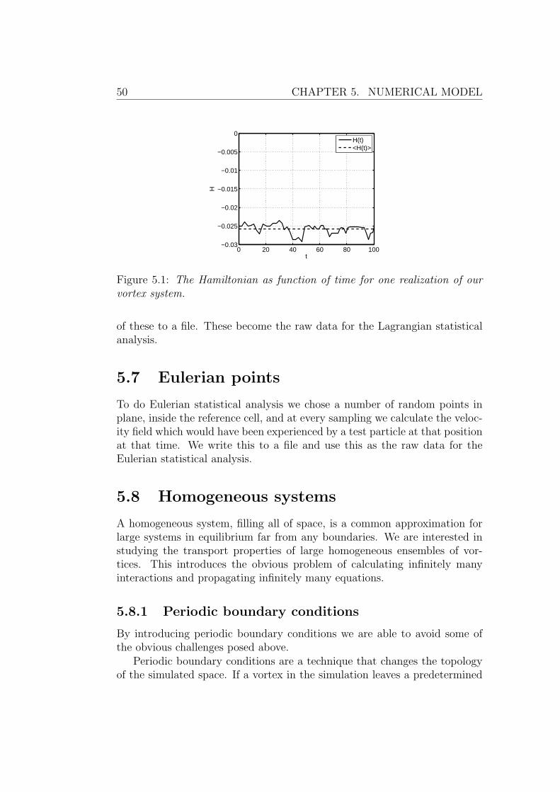
50 CHAPTER 5. NUMERICAL MODEL
0 20 40 60 80 100−0.03
−0.025
−0.02
−0.015
−0.01
−0.005
0
t
H
H(t)<H(t)>
Figure 5.1: The Hamiltonian as function of time for one realization of ourvortex system.
of these to a file. These become the raw data for the Lagrangian statisticalanalysis.
5.7 Eulerian points
To do Eulerian statistical analysis we chose a number of random points inplane, inside the reference cell, and at every sampling we calculate the veloc-ity field which would have been experienced by a test particle at that positionat that time. We write this to a file and use this as the raw data for theEulerian statistical analysis.
5.8 Homogeneous systems
A homogeneous system, filling all of space, is a common approximation forlarge systems in equilibrium far from any boundaries. We are interested instudying the transport properties of large homogeneous ensembles of vor-tices. This introduces the obvious problem of calculating infinitely manyinteractions and propagating infinitely many equations.
5.8.1 Periodic boundary conditions
By introducing periodic boundary conditions we are able to avoid some ofthe obvious challenges posed above.
Periodic boundary conditions are a technique that changes the topologyof the simulated space. If a vortex in the simulation leaves a predetermined
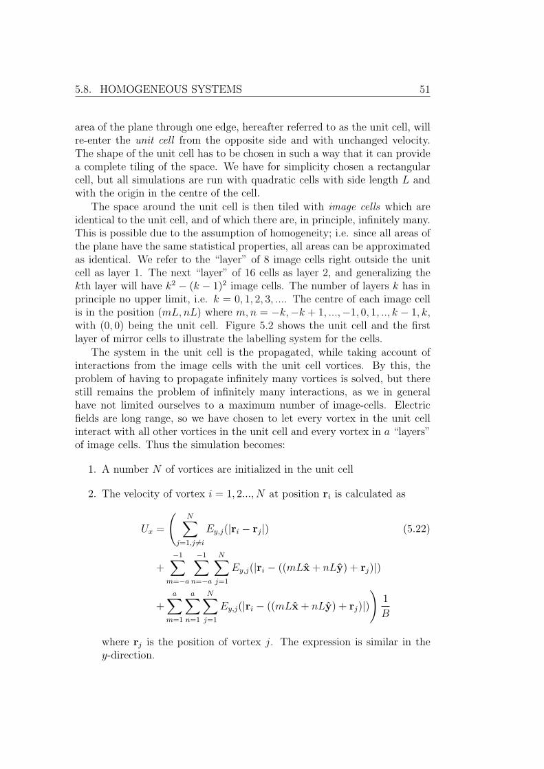
5.8. HOMOGENEOUS SYSTEMS 51
area of the plane through one edge, hereafter referred to as the unit cell, willre-enter the unit cell from the opposite side and with unchanged velocity.The shape of the unit cell has to be chosen in such a way that it can providea complete tiling of the space. We have for simplicity chosen a rectangularcell, but all simulations are run with quadratic cells with side length L andwith the origin in the centre of the cell.
The space around the unit cell is then tiled with image cells which areidentical to the unit cell, and of which there are, in principle, infinitely many.This is possible due to the assumption of homogeneity; i.e. since all areas ofthe plane have the same statistical properties, all areas can be approximatedas identical. We refer to the “layer” of 8 image cells right outside the unitcell as layer 1. The next “layer” of 16 cells as layer 2, and generalizing thekth layer will have k2 − (k − 1)2 image cells. The number of layers k has inprinciple no upper limit, i.e. k = 0, 1, 2, 3, .... The centre of each image cellis in the position (mL, nL) where m,n = −k,−k + 1, ...,−1, 0, 1, .., k − 1, k,with (0, 0) being the unit cell. Figure 5.2 shows the unit cell and the firstlayer of mirror cells to illustrate the labelling system for the cells.
The system in the unit cell is the propagated, while taking account ofinteractions from the image cells with the unit cell vortices. By this, theproblem of having to propagate infinitely many vortices is solved, but therestill remains the problem of infinitely many interactions, as we in generalhave not limited ourselves to a maximum number of image-cells. Electricfields are long range, so we have chosen to let every vortex in the unit cellinteract with all other vortices in the unit cell and every vortex in a “layers”of image cells. Thus the simulation becomes:
1. A number N of vortices are initialized in the unit cell
2. The velocity of vortex i = 1, 2..., N at position ri is calculated as
Ux =
(N∑
j=1,j 6=i
Ey,j(|ri − rj|) (5.22)
+−1∑
m=−a
−1∑n=−a
N∑j=1
Ey,j(|ri − ((mLx + nLy) + rj)|)
+a∑
m=1
a∑n=1
N∑j=1
Ey,j(|ri − ((mLx + nLy) + rj)|)
)1
B
where rj is the position of vortex j. The expression is similar in they-direction.
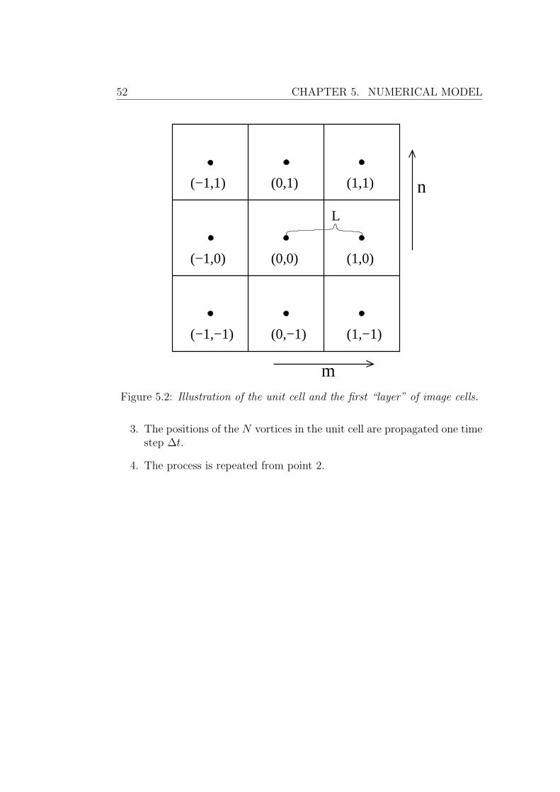
52 CHAPTER 5. NUMERICAL MODEL
(−1,1) (0,1) (1,1)
(1,0)(0,0)(−1,0)
(−1,−1) (0,−1) (1,−1)
L
m
n
Figure 5.2: Illustration of the unit cell and the first “layer” of image cells.
3. The positions of the N vortices in the unit cell are propagated one timestep ∆t.
4. The process is repeated from point 2.
Chapter 6
Data analysis
For the purpose of analysing the simulations, we made datasets from eachrun. The main variables contained in these datasets was the position of eachvortex, the positions and velocities of the test vortices and the velocity ateach of the Eulerian points at every sampling time. We have used these tostudy the time evolution of the vortex systems from several different initialconditions. The main focus of this study is the characterisation of the trans-port properties of a random vortex ensemble, both infinite and localized.
6.1 Density histograms
A basic characteristic of a localized system is it’s spatial distribution as afunction of time. To study this we have made density histograms, whichshow the particle density in a particular area of space at the sampling time
The density histograms are made with a two dimensional histogram rou-tine resulting in plots as shown in Figure 7.1. Temporal evolutions can betracked through comparisons of diagrams taken at selected times.
6.2 Ensemble mean values
The raw data are used to directly calculate the first order moment 〈|r|〉 andthe second order 〈r2〉 moments, respectively, of the spatial distribution atevery sampling time. These characterize the average time evolution of thelocalized ensembles. The second order moment is the variance of the spatialdistribution, given that 〈r〉 = 0, which is the case here, while 〈|r|〉 is alsoa measure of the spread of the distribution, but without obvious physicalmeaning.
53
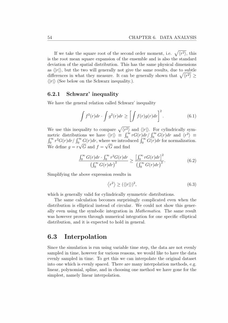
54 CHAPTER 6. DATA ANALYSIS
If we take the square root of the second order moment, i.e.√〈r2〉, this
is the root mean square expansion of the ensemble and is also the standarddeviation of the spatial distribution. This has the same physical dimensionsas 〈|r|〉, but the two will generally not give the same results, due to subtledifferences in what they measure. It can be generally shown that
√〈r2〉 ≥
〈|r|〉 (See below on the Schwarz inequality.).
6.2.1 Schwarz’ inequality
We have the general relation called Schwarz’ inequality∫f 2(r)dr ·
∫g2(r)dr ≥
[∫f(r)g(r)dr
]2
. (6.1)
We use this inequality to compare√〈r2〉 and 〈|r|〉. For cylindrically sym-
metric distributions we have 〈|r|〉 ≡∫∞
0rG(r)dr/
∫∞0G(r)dr and 〈r2〉 ≡∫∞
0r2G(r)dr/
∫∞0G(r)dr, where we introduced
∫∞0G(r)dr for normalization.
We define g = r√G and f =
√G and find∫∞
0G(r)dr ·
∫∞0r2G(r)dr(∫∞
0G(r)dr
)2 ≥[∫∞
0rG(r)dr
]2(∫∞0G(r)dr
)2 . (6.2)
Simplifying the above expression results in⟨r2⟩≥ (〈|r|〉)2, (6.3)
which is generally valid for cylindrically symmetric distributions.The same calculation becomes surprisingly complicated even when the
distribution is elliptical instead of circular. We could not show this gener-ally even using the symbolic integration in Mathematica. The same resultwas however proven through numerical integration for one specific ellipticaldistribution, and it is expected to hold in general.
6.3 Interpolation
Since the simulation is run using variable time step, the data are not evenlysampled in time, however for various reasons, we would like to have the dataevenly sampled in time. To get this we can interpolate the original datasetinto one which is evenly spaced. There are many interpolation methods, e.g.linear, polynomial, spline, and in choosing one method we have gone for thesimplest, namely linear interpolation.
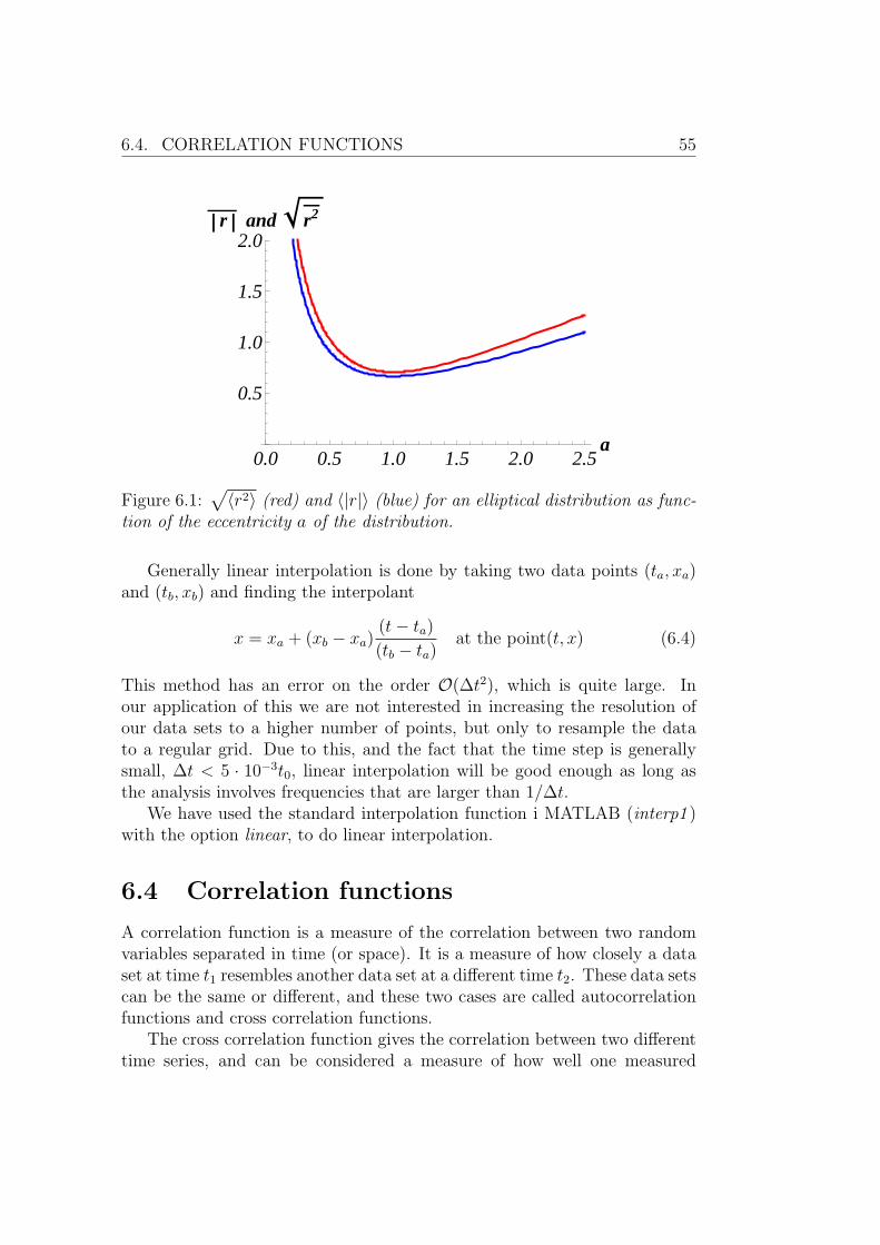
6.4. CORRELATION FUNCTIONS 55
0.0 0.5 1.0 1.5 2.0 2.5a
0.5
1.0
1.5
2.0r and r2
Figure 6.1:√〈r2〉 (red) and 〈|r|〉 (blue) for an elliptical distribution as func-
tion of the eccentricity a of the distribution.
Generally linear interpolation is done by taking two data points (ta, xa)and (tb, xb) and finding the interpolant
x = xa + (xb − xa)(t− ta)(tb − ta)
at the point(t, x) (6.4)
This method has an error on the order O(∆t2), which is quite large. Inour application of this we are not interested in increasing the resolution ofour data sets to a higher number of points, but only to resample the datato a regular grid. Due to this, and the fact that the time step is generallysmall, ∆t < 5 · 10−3t0, linear interpolation will be good enough as long asthe analysis involves frequencies that are larger than 1/∆t.
We have used the standard interpolation function i MATLAB (interp1 )with the option linear, to do linear interpolation.
6.4 Correlation functions
A correlation function is a measure of the correlation between two randomvariables separated in time (or space). It is a measure of how closely a dataset at time t1 resembles another data set at a different time t2. These data setscan be the same or different, and these two cases are called autocorrelationfunctions and cross correlation functions.
The cross correlation function gives the correlation between two differenttime series, and can be considered a measure of how well one measured
56 CHAPTER 6. DATA ANALYSIS
quantity can be used to predict the development of another; it is importantto remember that we do not necessarily know which quantity is cause andwhich is effect. The cross correlation function is defined as
C(t1, t2) =〈X(t1)Y (t2)〉√〈X2〉〈Y 2〉
(6.5)
where X(t), Y (t) are two different data sets; 〈X(t1)Y (t2)〉 is the covarianceof X and Y .
The autocorrelation function is the cross correlation between a time se-ries and itself, and gives the correlation between two points from the samedataset at different points in time. It can be considered as a measure of howwell measurements of one quantity at earlier times can be used to predictthe development of the same quantity at later times. The autocorrelationfunction is defined similarly
C(t1, t2) =〈X(t1)X(t2)〉〈X2〉
. (6.6)
If the random process measured is time stationary, we can simplify theabove expressions by introducing τ which denotes the time difference betweent1 and t2, i.e. τ = t2− t1. We are mainly interested in calculating correlationfunctions for the simulated infinite systems and assuming a time stationaryprocess seems reasonable in that case, since an infinite system in equilibriumis per definition time stationary. The new expression for the cross correlationbecomes
CXY (τ) =〈X(t)Y (t+ τ)〉√〈X2〉 〈Y 2〉
. (6.7)
The autocorrelation is then similarly
CXX(τ) =〈X(t+ τ)X(t)〉
〈X2〉. (6.8)
The discretized expression for the cross correlation functions is
CXY =1
n−τ∑n−τ
1=1 X(i)Y (i+ τ)√〈X2〉 〈Y 2〉
(6.9)
and equivalently for the autocorrelation function.The expressions above give the correlation functions between two time
series. Since we have several datasets, it will be convenient to combine theresults into one correlation function. The correct way to find this for m
6.4. CORRELATION FUNCTIONS 57
datasets is given below, where the covariance between the two variables Xand Y and the mean squares of X and Y are found separately.
CXY (τ) =
1m
∑mj=1
(1
n−τ∑n−τ
1=1 X(i)Y (i+ τ))j√
1m2
∑mj=1 〈X2〉j
∑mj=1 〈Y 2〉j
(6.10)
Physically, the correlation function quantifies how the processes whichgenerate a signal are related, and the ability to use one signal to predict orexplain the variation in in the same or another signal. For the autocorrelationfunction this relation is always greatest for τ = 0. The cross correlationfunction can have it’s maximum value for any τ depending on how the twoprocesses are related. The correlation functions contain physical informationon e.g. time scales of a process or the delay between two related processes.
In the current study it will be most interesting to investigate how the ve-locity of a test particle (u(r(t), t)) is correlated with itself, and the differencebetween the velocity autocorrelation function of test particles and veloc-ity autocorrelation functions of Eulerian points (autocorrelation of u(r, t)).These two different autocorrelation functions are called, respectively, theLagrangian velocity autocorrelation function and the Eulerian velocity auto-correlation function, and their theoretical differences are discussed in detailin Chapter 4
For a time stationary process the autocorrelation function is symmetricaround τ = 0. If we calculate the Fourier transform of the autocorrelationfunction this symmetry results in a Fourier transform which is real and pos-itive for all frequencies. This is the power spectrum of this variable. Thepower spectrum gives information about the frequencies of the energy con-taining processes in the system. From Section 4.2.1 we remember that thepower at frequency ω = 0 gives the Lagrangian integral correlation time τL.
Since we will have finite length time series of data, the autocorrelationfunctions for high time lag τ will be quite noisy. To avoid having this intro-ducing spurious fluctuations in the power spectra, we will only use the first2/3s of the autocorrelation functions when calculation the power spectra.
A finite number of realizations, such as we have here, can only provide anestimate of the average, not the true values. To quantify the error done byhaving a finite number of realizations can be found through the following:
Consider a random variable x and assume that you have found an estimate1N
∑Nj=1 xj for the average µ ≡ 〈x〉. The error e on the estimate is given as
e ≡
⟨(〈x〉 − 1
N
N∑j=1
xj
)2⟩. (6.11)
58 CHAPTER 6. DATA ANALYSIS
This results in
e = 〈x〉2 +1
N2
⟨(N∑j=1
xj
)2⟩− 2
⟨〈x〉 1
N
N∑j=1
xj
⟩.
The last term can be written as −2 〈x〉2, while the second term can be writtenas
1
N2
N∑k=1
N∑j=1
〈xjxk〉 .
This double sum contains N terms where j = k, all of which results in⟨x2j
⟩= 〈x2〉, and N(N − 1) terms where j 6= k. The latter can be written as
〈xjxk〉 = 〈xj〉 〈xk〉 = 〈x〉2. Combining these terms again, our error e is
e = 〈x〉2 +1
N2(N⟨x2⟩
+N(N − 1) 〈x〉2)− 2 〈x〉2 .
Simplifying results in
e =1
N(⟨x2⟩− 〈x〉2).
For N → ∞ we have e → 0 as expected in such a way that the root-mean-square error decreases as 1/
√N . The discussion can be extended to
other, also higher order, averages and correlations, but the expressions be-come lengthy.
6.5 Probability density functions
The measured time series can be difficult to interpret in their raw state.To get an overall impression of the data we have estimated the probabilitydensity function (PDF) of the data for the Lagrangian and Eulerian velocitystatistics. To do this we grouped the data into bins and counted the numberof observations in each bin, just as one would for making a histogram. Theresult was the normalized to ensure that the area under the graph was equalto one.
Chapter 7
Results
In this chapter we present the results from the numerical experiments con-ducted. All results are obtained from simulations done with the code de-scribed in Chapter 5.
First we present results concerning the time evolution of a localized ran-dom ensemble of N vortices with net vorticity density 1
N
∑i γi. We present
the results for several different initial conditions.Next we will study a generalization of the four vortex collisions from
section 3.2.3. We generalize this to four ensembles with N = 100 individualvortices in each, and we will classify the behaviour in terms of the impactparameter b.
Last we present the results from simulations of homogeneous systems interms of a turbulent velocity field, as discussed in Chapter 4, by using theboundary conditions presented in section 5.8.
7.1 Time evolution of a localized random en-
semble
The basic behaviour of such systems depends on the sign and distribution ofthe vortex strengths. We adopt the notation χ ∼ D(a, b) where the variableχ is a stochastic variable with distribution D(a, b). The relevant cases are
1. All vortices have the same sign
All vortices have the same sign and strength, set to 1.
The vortex strengths are distributed γ ∼ U(0, 1)1. Here U(a, b)
1In all these cases P (γ = 0) = 0 since vortices with γ = 0 will be completely inert.Simulating these will be a waste of computational resources.
59
60 CHAPTER 7. RESULTS
represent the uniform distribution on the interval (a, b)
2. The vortex strengths are randomly distributed with mean 0 so that thetotal vorticity is 1
N
∑i γi ≈ 0.
The strengths are distributed so that P (γ = 1) = P (γ = −1) =1/2.
The strengths are distributed γ ∼ U(−1, 1)1.
The strengths are distributed γ ∼ N(0, 1/2)1. Here N(a, b) repre-sents the Normal distribution with µ = a and σ = b.
The cases have been simulated using the code described in Chapter 5, andthe simulations have been done for both unshielded and shielded vortices aswell as for both circular and elliptical spatial distributions. The circulardistributions are exact solutions of the equations (3.6) and (3.7), while theelliptical distributions are not. Density histograms of these simulations areshown in Figures 7.1-7.4). The cases shown here are illustrative: Circularand elliptical distribution with P (γ) = 1; circular and elliptical distributionwith P (γ = 1) = P (γ = −1) = 1/2. The illustrations are for unshieldedvortex potentials.
The basic behaviour is, as previously stated, strongly dependent on thesign distribution of the systems and on the presence of shielding. Whenall vortices have the same sign, the dominating behaviour is a large scalerotation of the entire system, similar to the two vortex dynamics for samesign vortices. There is very little expansion of the system in these cases,especially for the circular distributions.
The elliptical distributions are stretched by the rotation, and the outerparts of the ellipse are thrown away from the central rotating core, whichrapidly becomes circular.
When shielding effects have been included, and with spatial distributionsignificantly larger than the Debye length, the result is no large scale coherentmotion, only small scale fluctuating interactions.
When the vortices have different polarity and the net vorticity densityis approximately zero, there is no net rotation of the system, instead thesmall scale interactions between nearby vortices dominate, and the pairingup of two vortices of opposite polarity results in a large of expansion of theseclouds. The cloud quickly loses it’s character. This general behaviour is validboth for circular, and elliptic clouds and for both shielded and unshieldedvortices. The result here is visually similar to the turbulent diffusion illus-trated in Figure 4.1. The distortion of the cloud of vortices is much larger
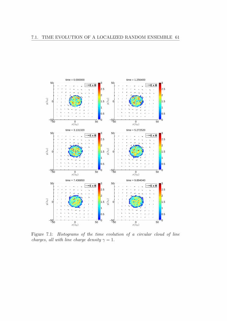
7.1. TIME EVOLUTION OF A LOCALIZED RANDOM ENSEMBLE 61
−50 0 50−50
0
50
x(λD)
time = 0.000000
y(λ
D)
0
0.5
1
1.5
2
2.5
3E x B
−50 0 50−50
0
50
x(λD)
time = 1.256400
y(λ
D)
0
0.5
1
1.5
2
2.5
3E x B
−50 0 50−50
0
50
x(λD)
time = 3.131320
y(λ
D)
0
0.5
1
1.5
2
2.5
3E x B
−50 0 50−50
0
50
x(λD)
time = 5.272520
y(λ
D)
0
0.5
1
1.5
2
2.5
3E x B
−50 0 50−50
0
50
x(λD)
time = 7.436850
y(λ
D)
0
0.5
1
1.5
2
2.5
3E x B
−50 0 50−50
0
50
x(λD)
time = 9.894040
y(λ
D)
0
0.5
1
1.5
2
2.5
3E x B
Figure 7.1: Histograms of the time evolution of a circular cloud of linecharges, all with line charge density γ = 1.
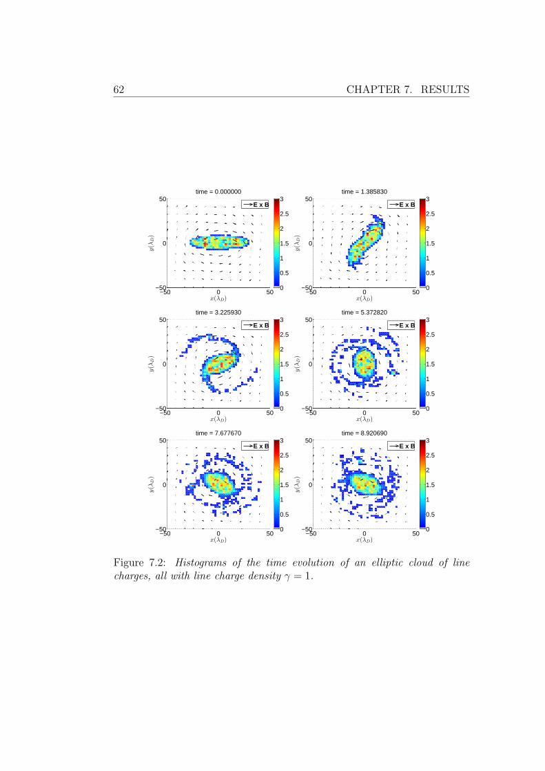
62 CHAPTER 7. RESULTS
−50 0 50−50
0
50
x(λD)
time = 0.000000
y(λ
D)
0
0.5
1
1.5
2
2.5
3E x B
−50 0 50−50
0
50
x(λD)
time = 1.385830
y(λ
D)
0
0.5
1
1.5
2
2.5
3E x B
−50 0 50−50
0
50
x(λD)
time = 3.225930
y(λ
D)
0
0.5
1
1.5
2
2.5
3E x B
−50 0 50−50
0
50
x(λD)
time = 5.372820
y(λ
D)
0
0.5
1
1.5
2
2.5
3E x B
−50 0 50−50
0
50
x(λD)
time = 7.677670
y(λ
D)
0
0.5
1
1.5
2
2.5
3E x B
−50 0 50−50
0
50
x(λD)
time = 8.920690
y(λ
D)
0
0.5
1
1.5
2
2.5
3E x B
Figure 7.2: Histograms of the time evolution of an elliptic cloud of linecharges, all with line charge density γ = 1.
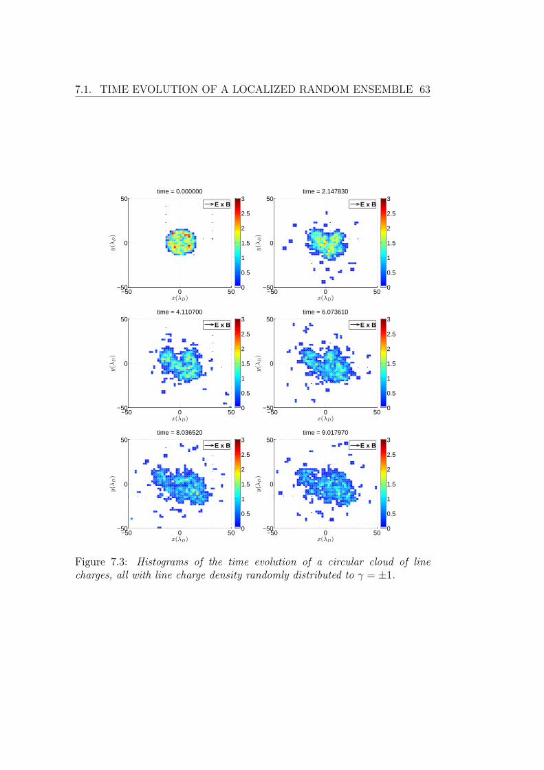
7.1. TIME EVOLUTION OF A LOCALIZED RANDOM ENSEMBLE 63
−50 0 50−50
0
50
x(λD)
time = 0.000000
y(λ
D)
0
0.5
1
1.5
2
2.5
3E x B
−50 0 50−50
0
50
x(λD)
time = 2.147830
y(λ
D)
0
0.5
1
1.5
2
2.5
3E x B
−50 0 50−50
0
50
x(λD)
time = 4.110700
y(λ
D)
0
0.5
1
1.5
2
2.5
3E x B
−50 0 50−50
0
50
x(λD)
time = 6.073610
y(λ
D)
0
0.5
1
1.5
2
2.5
3E x B
−50 0 50−50
0
50
x(λD)
time = 8.036520
y(λ
D)
0
0.5
1
1.5
2
2.5
3E x B
−50 0 50−50
0
50
x(λD)
time = 9.017970
y(λ
D)
0
0.5
1
1.5
2
2.5
3E x B
Figure 7.3: Histograms of the time evolution of a circular cloud of linecharges, all with line charge density randomly distributed to γ = ±1.
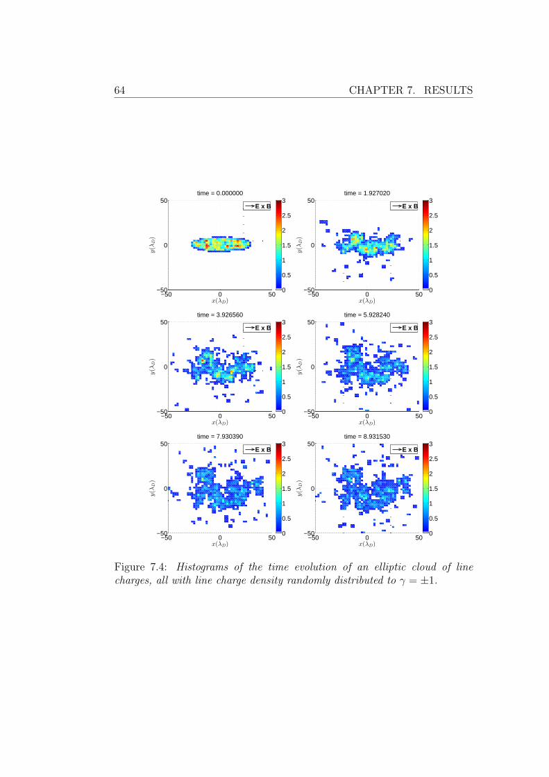
64 CHAPTER 7. RESULTS
−50 0 50−50
0
50
x(λD)
time = 0.000000
y(λ
D)
0
0.5
1
1.5
2
2.5
3E x B
−50 0 50−50
0
50
x(λD)
time = 1.927020
y(λ
D)
0
0.5
1
1.5
2
2.5
3E x B
−50 0 50−50
0
50
x(λD)
time = 3.926560
y(λ
D)
0
0.5
1
1.5
2
2.5
3E x B
−50 0 50−50
0
50
x(λD)
time = 5.928240
y(λ
D)
0
0.5
1
1.5
2
2.5
3E x B
−50 0 50−50
0
50
x(λD)
time = 7.930390
y(λ
D)
0
0.5
1
1.5
2
2.5
3E x B
−50 0 50−50
0
50
x(λD)
time = 8.931530
y(λ
D)
0
0.5
1
1.5
2
2.5
3E x B
Figure 7.4: Histograms of the time evolution of an elliptic cloud of linecharges, all with line charge density randomly distributed to γ = ±1.
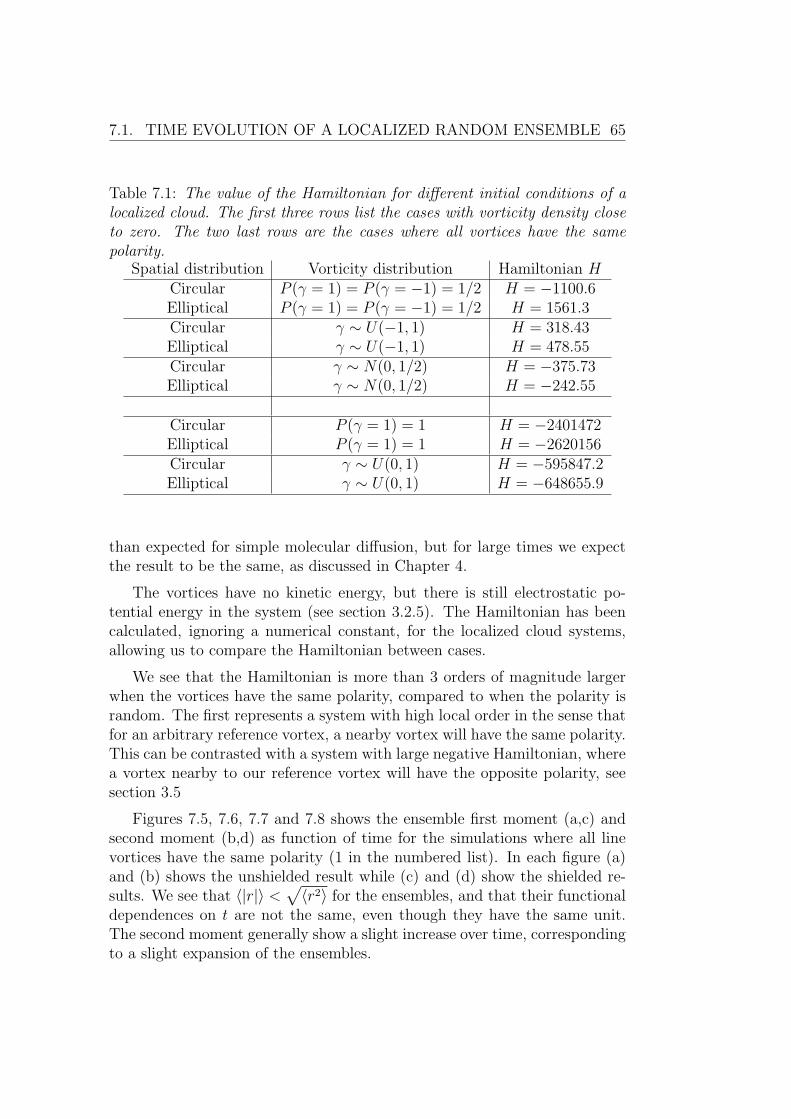
7.1. TIME EVOLUTION OF A LOCALIZED RANDOM ENSEMBLE 65
Table 7.1: The value of the Hamiltonian for different initial conditions of alocalized cloud. The first three rows list the cases with vorticity density closeto zero. The two last rows are the cases where all vortices have the samepolarity.
Spatial distribution Vorticity distribution Hamiltonian HCircular P (γ = 1) = P (γ = −1) = 1/2 H = −1100.6Elliptical P (γ = 1) = P (γ = −1) = 1/2 H = 1561.3Circular γ ∼ U(−1, 1) H = 318.43Elliptical γ ∼ U(−1, 1) H = 478.55Circular γ ∼ N(0, 1/2) H = −375.73Elliptical γ ∼ N(0, 1/2) H = −242.55
Circular P (γ = 1) = 1 H = −2401472Elliptical P (γ = 1) = 1 H = −2620156Circular γ ∼ U(0, 1) H = −595847.2Elliptical γ ∼ U(0, 1) H = −648655.9
than expected for simple molecular diffusion, but for large times we expectthe result to be the same, as discussed in Chapter 4.
The vortices have no kinetic energy, but there is still electrostatic po-tential energy in the system (see section 3.2.5). The Hamiltonian has beencalculated, ignoring a numerical constant, for the localized cloud systems,allowing us to compare the Hamiltonian between cases.
We see that the Hamiltonian is more than 3 orders of magnitude largerwhen the vortices have the same polarity, compared to when the polarity israndom. The first represents a system with high local order in the sense thatfor an arbitrary reference vortex, a nearby vortex will have the same polarity.This can be contrasted with a system with large negative Hamiltonian, wherea vortex nearby to our reference vortex will have the opposite polarity, seesection 3.5
Figures 7.5, 7.6, 7.7 and 7.8 shows the ensemble first moment (a,c) andsecond moment (b,d) as function of time for the simulations where all linevortices have the same polarity (1 in the numbered list). In each figure (a)and (b) shows the unshielded result while (c) and (d) show the shielded re-sults. We see that 〈|r|〉 <
√〈r2〉 for the ensembles, and that their functional
dependences on t are not the same, even though they have the same unit.The second moment generally show a slight increase over time, correspondingto a slight expansion of the ensembles.
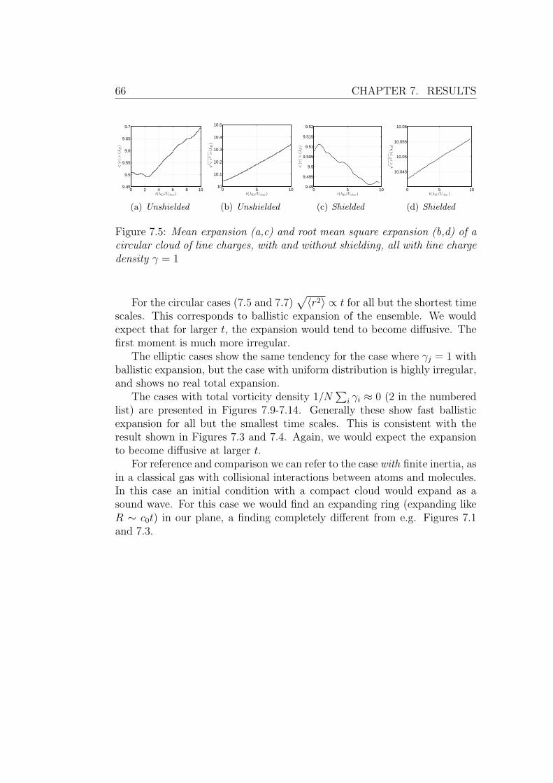
66 CHAPTER 7. RESULTS
0 2 4 6 8 109.45
9.5
9.55
9.6
9.65
9.7
t(λD/Uchar)
<|r|>
(λD)
(a) Unshielded
0 5 1010
10.1
10.2
10.3
10.4
10.5
t(λD/Uchar)
√
<r2
>(λ
D)
(b) Unshielded
0 5 109.49
9.495
9.5
9.505
9.51
9.515
9.52
t(λD/Uchar)
<|r|>
(λD)
(c) Shielded
0 5 10
10.045
10.05
10.055
10.06
t(λD/Uchar)
√
<r2
>(λ
D)
(d) Shielded
Figure 7.5: Mean expansion (a,c) and root mean square expansion (b,d) of acircular cloud of line charges, with and without shielding, all with line chargedensity γ = 1
For the circular cases (7.5 and 7.7)√〈r2〉 ∝ t for all but the shortest time
scales. This corresponds to ballistic expansion of the ensemble. We wouldexpect that for larger t, the expansion would tend to become diffusive. Thefirst moment is much more irregular.
The elliptic cases show the same tendency for the case where γj = 1 withballistic expansion, but the case with uniform distribution is highly irregular,and shows no real total expansion.
The cases with total vorticity density 1/N∑
i γi ≈ 0 (2 in the numberedlist) are presented in Figures 7.9-7.14. Generally these show fast ballisticexpansion for all but the smallest time scales. This is consistent with theresult shown in Figures 7.3 and 7.4. Again, we would expect the expansionto become diffusive at larger t.
For reference and comparison we can refer to the case with finite inertia, asin a classical gas with collisional interactions between atoms and molecules.In this case an initial condition with a compact cloud would expand as asound wave. For this case we would find an expanding ring (expanding likeR ∼ c0t) in our plane, a finding completely different from e.g. Figures 7.1and 7.3.
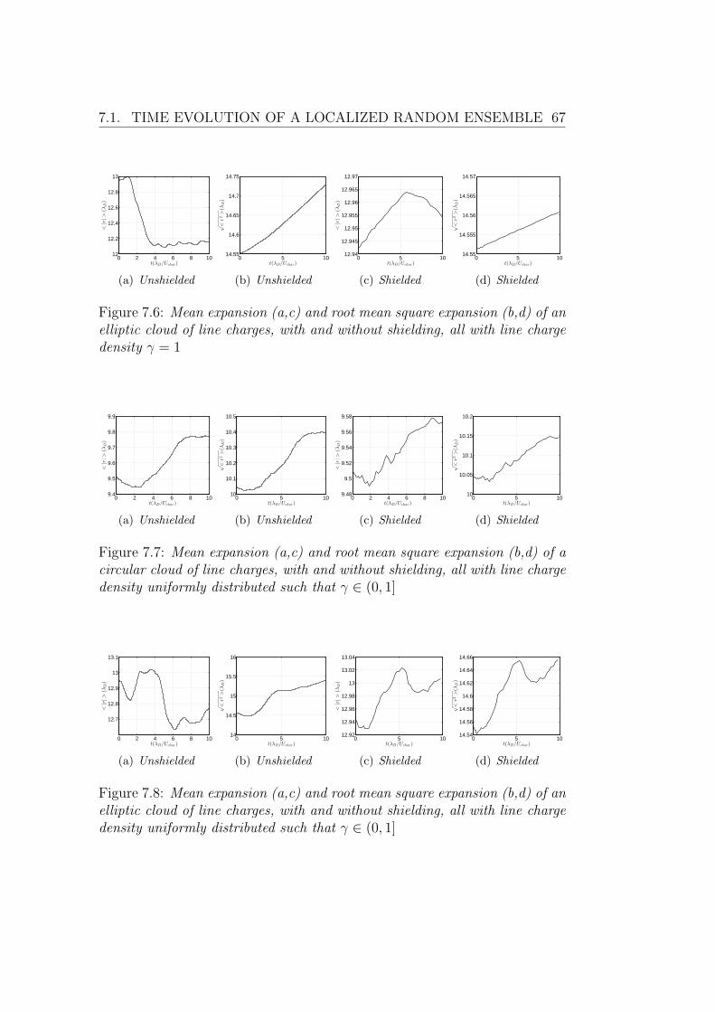
7.1. TIME EVOLUTION OF A LOCALIZED RANDOM ENSEMBLE 67
0 2 4 6 8 1012
12.2
12.4
12.6
12.8
13
t(λD/Uchar)
<|r|>
(λD)
(a) Unshielded
0 5 1014.55
14.6
14.65
14.7
14.75
t(λD/Uchar)
√
<r2
>(λ
D)
(b) Unshielded
0 5 1012.94
12.945
12.95
12.955
12.96
12.965
12.97
t(λD/Uchar)
<|r|>
(λD)
(c) Shielded
0 5 1014.55
14.555
14.56
14.565
14.57
t(λD/Uchar)
√
<r2
>(λ
D)
(d) Shielded
Figure 7.6: Mean expansion (a,c) and root mean square expansion (b,d) of anelliptic cloud of line charges, with and without shielding, all with line chargedensity γ = 1
0 2 4 6 8 109.4
9.5
9.6
9.7
9.8
9.9
t(λD/Uchar)
<|r|>
(λD)
(a) Unshielded
0 5 1010
10.1
10.2
10.3
10.4
10.5
t(λD/Uchar)
√
<r2
>(λ
D)
(b) Unshielded
0 2 4 6 8 109.48
9.5
9.52
9.54
9.56
9.58
t(λD/Uchar)
<|r|>
(λD)
(c) Shielded
0 5 1010
10.05
10.1
10.15
10.2
t(λD/Uchar)
√
<r2
>(λ
D)
(d) Shielded
Figure 7.7: Mean expansion (a,c) and root mean square expansion (b,d) of acircular cloud of line charges, with and without shielding, all with line chargedensity uniformly distributed such that γ ∈ (0, 1]
0 2 4 6 8 10
12.7
12.8
12.9
13
13.1
t(λD/Uchar)
<|r|>
(λD)
(a) Unshielded
0 5 1014
14.5
15
15.5
16
t(λD/Uchar)
√
<r2
>(λ
D)
(b) Unshielded
0 5 1012.92
12.94
12.96
12.98
13
13.02
13.04
t(λD/Uchar)
<|r|>
(λD)
(c) Shielded
0 5 1014.54
14.56
14.58
14.6
14.62
14.64
14.66
t(λD/Uchar)
√
<r2
>(λ
D)
(d) Shielded
Figure 7.8: Mean expansion (a,c) and root mean square expansion (b,d) of anelliptic cloud of line charges, with and without shielding, all with line chargedensity uniformly distributed such that γ ∈ (0, 1]
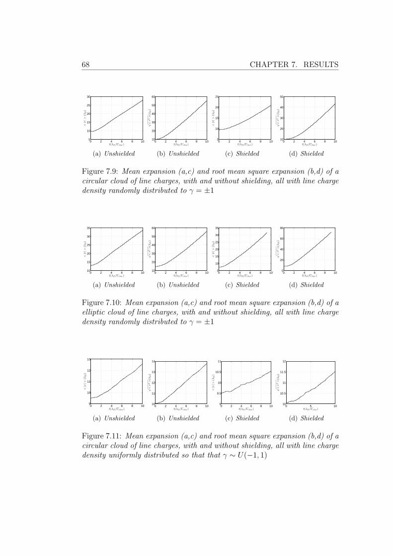
68 CHAPTER 7. RESULTS
0 2 4 6 8 105
10
15
20
25
30
t(λD/Uchar)
<|r|>
(λD)
(a) Unshielded
0 2 4 6 8 1010
20
30
40
50
60
t(λD/Uchar)√
<r2
>(λ
D)
(b) Unshielded
0 2 4 6 8 105
10
15
20
25
t(λD/Uchar)
<|r|>
(λD)
(c) Shielded
0 2 4 6 8 1010
20
30
40
50
t(λD/Uchar)
√
<r2
>(λ
D)
(d) Shielded
Figure 7.9: Mean expansion (a,c) and root mean square expansion (b,d) of acircular cloud of line charges, with and without shielding, all with line chargedensity randomly distributed to γ = ±1
0 2 4 6 8 1010
15
20
25
30
35
t(λD/Uchar)
<|r|>
(λD)
(a) Unshielded
0 2 4 6 8 1010
20
30
40
50
60
t(λD/Uchar)
√
<r2
>(λ
D)
(b) Unshielded
0 2 4 6 8 105
10
15
20
25
30
35
t(λD/Uchar)
<|r|>
(λD)
(c) Shielded
0 2 4 6 8 100
20
40
60
80
t(λD/Uchar)√
<r2
>(λ
D)
(d) Shielded
Figure 7.10: Mean expansion (a,c) and root mean square expansion (b,d) of aelliptic cloud of line charges, with and without shielding, all with line chargedensity randomly distributed to γ = ±1
0 2 4 6 8 109
10
11
12
13
t(λD/Uchar)
<|r|>
(λD)
(a) Unshielded
0 2 4 6 8 1010
11
12
13
14
t(λD/Uchar)
√
<r2
>(λ
D)
(b) Unshielded
0 2 4 6 8 109
9.5
10
10.5
11
t(λD/Uchar)
<|r|>
(λD)
(c) Shielded
0 5 1010
10.5
11
11.5
12
t(λD/Uchar)
√
<r2
>(λ
D)
(d) Shielded
Figure 7.11: Mean expansion (a,c) and root mean square expansion (b,d) of acircular cloud of line charges, with and without shielding, all with line chargedensity uniformly distributed so that that γ ∼ U(−1, 1)
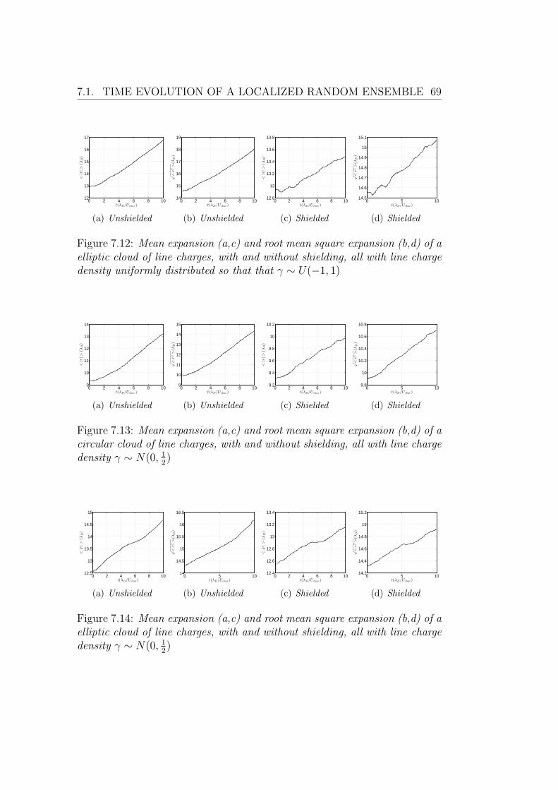
7.1. TIME EVOLUTION OF A LOCALIZED RANDOM ENSEMBLE 69
0 2 4 6 8 1012
13
14
15
16
17
t(λD/Uchar)
<|r|>
(λD)
(a) Unshielded
0 2 4 6 8 1014
15
16
17
18
19
t(λD/Uchar)
√
<r2
>(λ
D)
(b) Unshielded
0 2 4 6 8 1012.8
13
13.2
13.4
13.6
13.8
t(λD/Uchar)
<|r|>
(λD)
(c) Shielded
0 5 1014.5
14.6
14.7
14.8
14.9
15
15.1
t(λD/Uchar)
√
<r2
>(λ
D)
(d) Shielded
Figure 7.12: Mean expansion (a,c) and root mean square expansion (b,d) of aelliptic cloud of line charges, with and without shielding, all with line chargedensity uniformly distributed so that that γ ∼ U(−1, 1)
0 2 4 6 8 109
10
11
12
13
14
t(λD/Uchar)
<|r|>
(λD)
(a) Unshielded
0 2 4 6 8 109
10
11
12
13
14
15
t(λD/Uchar)
√
<r2
>(λ
D)
(b) Unshielded
0 2 4 6 8 109.2
9.4
9.6
9.8
10
10.2
t(λD/Uchar)
<|r|>
(λD)
(c) Shielded
0 5 109.8
10
10.2
10.4
10.6
10.8
t(λD/Uchar)
√
<r2
>(λ
D)
(d) Shielded
Figure 7.13: Mean expansion (a,c) and root mean square expansion (b,d) of acircular cloud of line charges, with and without shielding, all with line chargedensity γ ∼ N(0, 1
2)
0 2 4 6 8 1012.5
13
13.5
14
14.5
15
t(λD/Uchar)
<|r|>
(λD)
(a) Unshielded
0 5 1014
14.5
15
15.5
16
16.5
t(λD/Uchar)
√
<r2
>(λ
D)
(b) Unshielded
0 2 4 6 8 1012.4
12.6
12.8
13
13.2
13.4
t(λD/Uchar)
<|r|>
(λD)
(c) Shielded
0 5 1014.2
14.4
14.6
14.8
15
15.2
t(λD/Uchar)
√
<r2
>(λ
D)
(d) Shielded
Figure 7.14: Mean expansion (a,c) and root mean square expansion (b,d) of aelliptic cloud of line charges, with and without shielding, all with line chargedensity γ ∼ N(0, 1
2)
70 CHAPTER 7. RESULTS
7.2 Collisions of four vortex clouds
We have simulated the collision between four circular “clouds” of vortices,with two different radii, arranged similarly to the collisions discussed in Sec-tion 3.2.3. These single vortex collisions are the extreme limit of cloud colli-sions when the ratio of the cloud radius and the separation distance betweenclouds r/d→ 0. It can be interesting to note that a single pair will propagatein the same way as two point vortices, and that in a simulation of a singlepair, the individual clouds keep their separate identities for at least 500t0.
Samples of the space-time evolution of cloud pairs for selected parame-ters b and d (see Figure 7.15) are shown in Figures 7.16-7.19. Extracts ofparameters characterizing the final states are summarized in Tables 7.2 and7.3. These tables contain a wealth of information, which we believe can mostreadily be interpreted in terms of collisional cross sections. A part of thedata are extracted in Figure 7.20
In the simulation we held d = 20 fixed while we have varied the impactparameter b from 0 to 2d. This has been done for two different cloud radii,r1 = 1/2
√200 ≈ 7.07107 and r2 ≈
√200 = 14.14214 while the total number
of individual vortices was held constant at 401, i.e. 100 vortices in eachcloud, except for cloud 1, which for programming reasons has 101 individualvortices.
This system is a generalisation of the collision of two vortex pairs, dis-cussed in section 3.2.3, to distributions of vorticity. The point vortex collisionis the limit where r/d → 0. The greatest difference between the point vor-tex limit and the ensemble systems is the increasing number of degrees offreedom in the ensemble collisions. There is the centre of vorticity motionof each ensemble, the motion of individual line vortices around the ensemblecentre of vorticity, as well as the possibility of deformation and splitting ofthe ensembles.
The results of the simulations with ensemble radius r1 = 1/2√
200 ≈7.07107 for varying impact parameter b are presented in Figures 7.16 and7.17 and Table 7.2. Immediately we can see that the general behaviour canbe classified into several types, depending on b.
1. “Elastic” collisions, no excitation of other degrees of freedom than thecentre of vorticity motion. The vortex pairs interact and change part-ners in the same way as the individual vortices in section 3.2.3. Thiscan also be classified as collisions with deflections of 90 deg or more.For b = 0 to b = 0.7d, Figures 7.16(a) and 7.16(b).
2. Almost elastic collisions, but with slight “inelaticity”, i.e. a few linevortices are separated from the original ensemble, or are exchanged
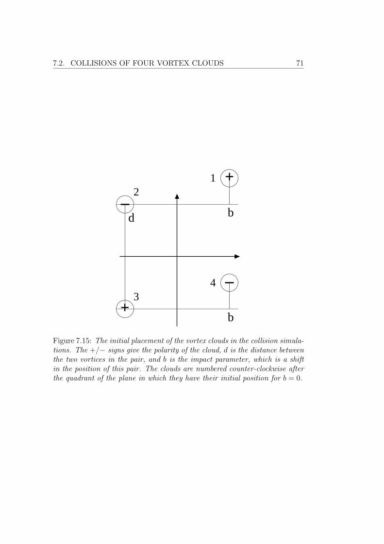
7.2. COLLISIONS OF FOUR VORTEX CLOUDS 71
+
+
b
b
d
1
43
2
Figure 7.15: The initial placement of the vortex clouds in the collision simula-tions. The +/− signs give the polarity of the cloud, d is the distance betweenthe two vortices in the pair, and b is the impact parameter, which is a shiftin the position of this pair. The clouds are numbered counter-clockwise afterthe quadrant of the plane in which they have their initial position for b = 0.
72 CHAPTER 7. RESULTS
between clouds. For b = 0.75d to b = 0.8d, Figures 7.16(c) and 7.16(d).
3. Ensemble 2 and 4 connect slightly, but split again. The two new pairsexit in quadrants 1 and 3. Many vortices are exchanged between 2 and4. For b = 0.85d. Not shown.
4. Inelastic collisions resulting in a bound state. Two ensembles withthe same polarity merge and produce a compound vortex of approxi-mately double strength. The two other two ensembles orbit the centralcombined vortex. The result is a stable tripolar vortex configurationresembling the tripolar vortices found experimentally and described byVranjes et al. (2002), Okamoto et al. (2003) and Okamoto et al. (2005).For b = 0.9d to b = 1.25d. The interesting observation here is that such“bound states” of three vortex clouds can result from an inelastic col-lision of four vortex clouds. Figures 7.16(e) and 7.16(f).
5. Strong interaction of the two ensembles with the same polarity result-ing in the formation of a combined central vortex, but the tripolarconfiguration is not stable, and the central vortex splits into two ap-proximately equal ensembles again. The result is the re-emergence oftwo pairs of ensembles. For b = 1.3d to b = 1.5d, Figures 7.17(a) and7.17(b).
6. A region of weaker interactions, with a few line vortices exchanged,but otherwise little deflection of the centre of vorticity motion. Forb = 1.55d to b = 1.95d, Figures 7.17(c) and 7.17(d).
7. Slight deflection of the centre of vorticity motion, but otherwise littleinteraction. For b = 2d, Figures 7.17(e) and 7.17(f).
8. When b d interactions will become negligible. Not shown.
The doubling of the ensemble radius, to r ≈√
200, while holding all otherparameters constant results in significantly altered behaviour. The resultsare presented in Figures 7.18 7.19 and Table 7.3. First we see that doublingthe radius means that there is an overlap between the component ensemblesof one pair and the density of line vortices is now reduced by a factor 4.
As shown in the figures, there is now no stable bound state, in contrastwith the result for clouds with half the radius. The individual line vorticesare more lightly bound to the ensemble of which they are part, and thusthe exchange and ejection of individual vortices happens for all values of b.The overall interaction between the centres of vorticity is less strong, and thebehaviour is in all cases less like the point vortex collisions.
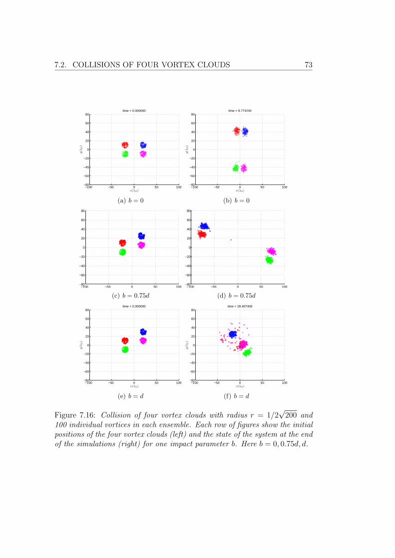
7.2. COLLISIONS OF FOUR VORTEX CLOUDS 73
−100 −50 0 50 100−80
−60
−40
−20
0
20
40
60
80time = 0.000000
x(λD)
y(λ
D)
(a) b = 0
−100 −50 0 50 100−80
−60
−40
−20
0
20
40
60
80time = 9.774240
x(λD)
y(λ
D)
(b) b = 0
−100 −50 0 50 100−80
−60
−40
−20
0
20
40
60
80
(c) b = 0.75d−100 −50 0 50 100
−80
−60
−40
−20
0
20
40
60
80
(d) b = 0.75d
−100 −50 0 50 100−80
−60
−40
−20
0
20
40
60
80time = 0.000000
x(λD)
y(λ
D)
(e) b = d
−100 −50 0 50 100−80
−60
−40
−20
0
20
40
60
80time = 39.407400
x(λD)
y(λ
D)
(f) b = d
Figure 7.16: Collision of four vortex clouds with radius r = 1/2√
200 and100 individual vortices in each ensemble. Each row of figures show the initialpositions of the four vortex clouds (left) and the state of the system at the endof the simulations (right) for one impact parameter b. Here b = 0, 0.75d, d.
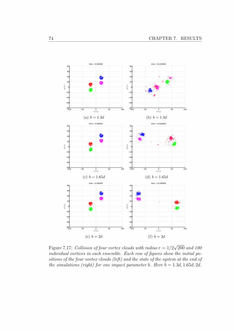
74 CHAPTER 7. RESULTS
−100 −50 0 50 100−80
−60
−40
−20
0
20
40
60
80time = 0.000000
x(λD)
y(λ
D)
(a) b = 1.3d
−100 −50 0 50 100−80
−60
−40
−20
0
20
40
60
80time = 19.245800
x(λD)
y(λ
D)
(b) b = 1.3d
−100 −50 0 50 100−80
−60
−40
−20
0
20
40
60
80time = 0.000000
x(λD)
y(λ
D)
(c) b = 1.65d
−100 −50 0 50 100−80
−60
−40
−20
0
20
40
60
80time = 19.039000
x(λD)
y(λ
D)
(d) b = 1.65d
−100 −50 0 50 100−80
−60
−40
−20
0
20
40
60
80time = 0.000000
x(λD)
y(λ
D)
(e) b = 2d
−100 −50 0 50 100−80
−60
−40
−20
0
20
40
60
80time = 19.249500
x(λD)
y(λ
D)
(f) b = 2d
Figure 7.17: Collision of four vortex clouds with radius r = 1/2√
200 and 100individual vortices in each ensemble. Each row of figures show the initial po-sitions of the four vortex clouds (left) and the state of the system at the end ofthe simulations (right) for one impact parameter b. Here b = 1.3d, 1.65d, 2d.
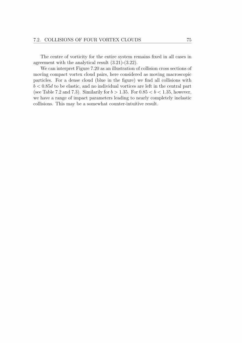
7.2. COLLISIONS OF FOUR VORTEX CLOUDS 75
The centre of vorticity for the entire system remains fixed in all cases inagreement with the analytical result (3.21)-(3.22).
We can interpret Figure 7.20 as an illustration of collision cross sections ofmoving compact vortex cloud pairs, here considered as moving macroscopicparticles. For a dense cloud (blue in the figure) we find all collisions withb < 0.85d to be elastic, and no individual vortices are left in the central part(see Table 7.2 and 7.3). Similarily for b > 1.35. For 0.85 < b < 1.35, however,we have a range of impact parameters leading to nearly completely inelasticcollisions. This may be a somewhat counter-intuitive result.
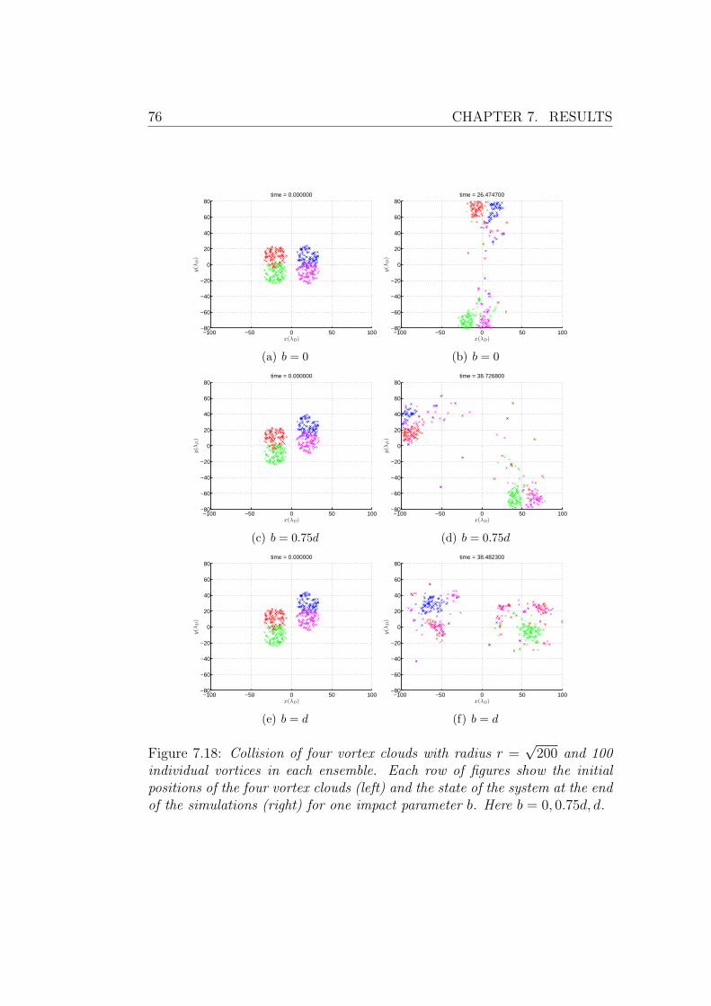
76 CHAPTER 7. RESULTS
−100 −50 0 50 100−80
−60
−40
−20
0
20
40
60
80time = 0.000000
x(λD)
y(λ
D)
(a) b = 0
−100 −50 0 50 100−80
−60
−40
−20
0
20
40
60
80time = 26.474700
x(λD)
y(λ
D)
(b) b = 0
−100 −50 0 50 100−80
−60
−40
−20
0
20
40
60
80time = 0.000000
x(λD)
y(λ
D)
(c) b = 0.75d
−100 −50 0 50 100−80
−60
−40
−20
0
20
40
60
80time = 38.726800
x(λD)
y(λ
D)
(d) b = 0.75d
−100 −50 0 50 100−80
−60
−40
−20
0
20
40
60
80time = 0.000000
x(λD)
y(λ
D)
(e) b = d
−100 −50 0 50 100−80
−60
−40
−20
0
20
40
60
80time = 38.482300
x(λD)
y(λ
D)
(f) b = d
Figure 7.18: Collision of four vortex clouds with radius r =√
200 and 100individual vortices in each ensemble. Each row of figures show the initialpositions of the four vortex clouds (left) and the state of the system at the endof the simulations (right) for one impact parameter b. Here b = 0, 0.75d, d.
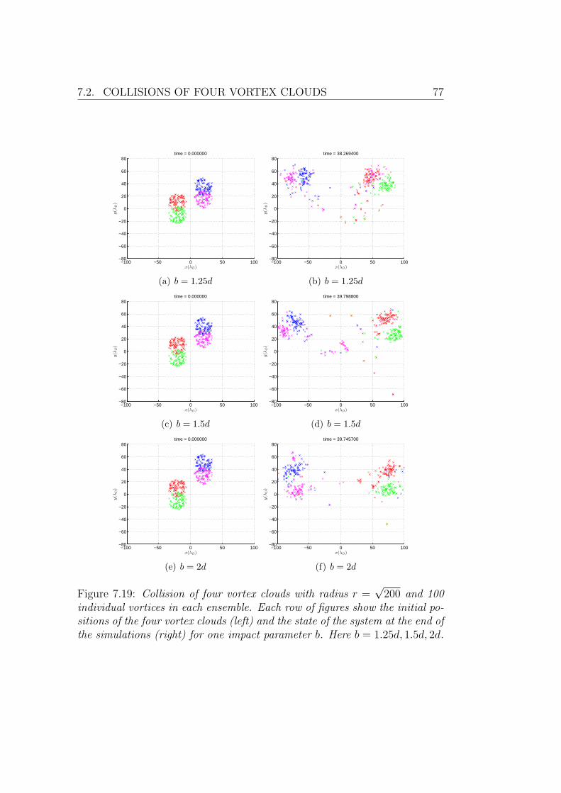
7.2. COLLISIONS OF FOUR VORTEX CLOUDS 77
−100 −50 0 50 100−80
−60
−40
−20
0
20
40
60
80time = 0.000000
x(λD)
y(λ
D)
(a) b = 1.25d
−100 −50 0 50 100−80
−60
−40
−20
0
20
40
60
80time = 38.269400
x(λD)y(λ
D)
(b) b = 1.25d
−100 −50 0 50 100−80
−60
−40
−20
0
20
40
60
80time = 0.000000
x(λD)
y(λ
D)
(c) b = 1.5d
−100 −50 0 50 100−80
−60
−40
−20
0
20
40
60
80time = 39.798800
x(λD)
y(λ
D)
(d) b = 1.5d
−100 −50 0 50 100−80
−60
−40
−20
0
20
40
60
80time = 0.000000
x(λD)
y(λ
D)
(e) b = 2d
−100 −50 0 50 100−80
−60
−40
−20
0
20
40
60
80time = 39.745700
x(λD)
y(λ
D)
(f) b = 2d
Figure 7.19: Collision of four vortex clouds with radius r =√
200 and 100individual vortices in each ensemble. Each row of figures show the initial po-sitions of the four vortex clouds (left) and the state of the system at the end ofthe simulations (right) for one impact parameter b. Here b = 1.25d, 1.5d, 2d.
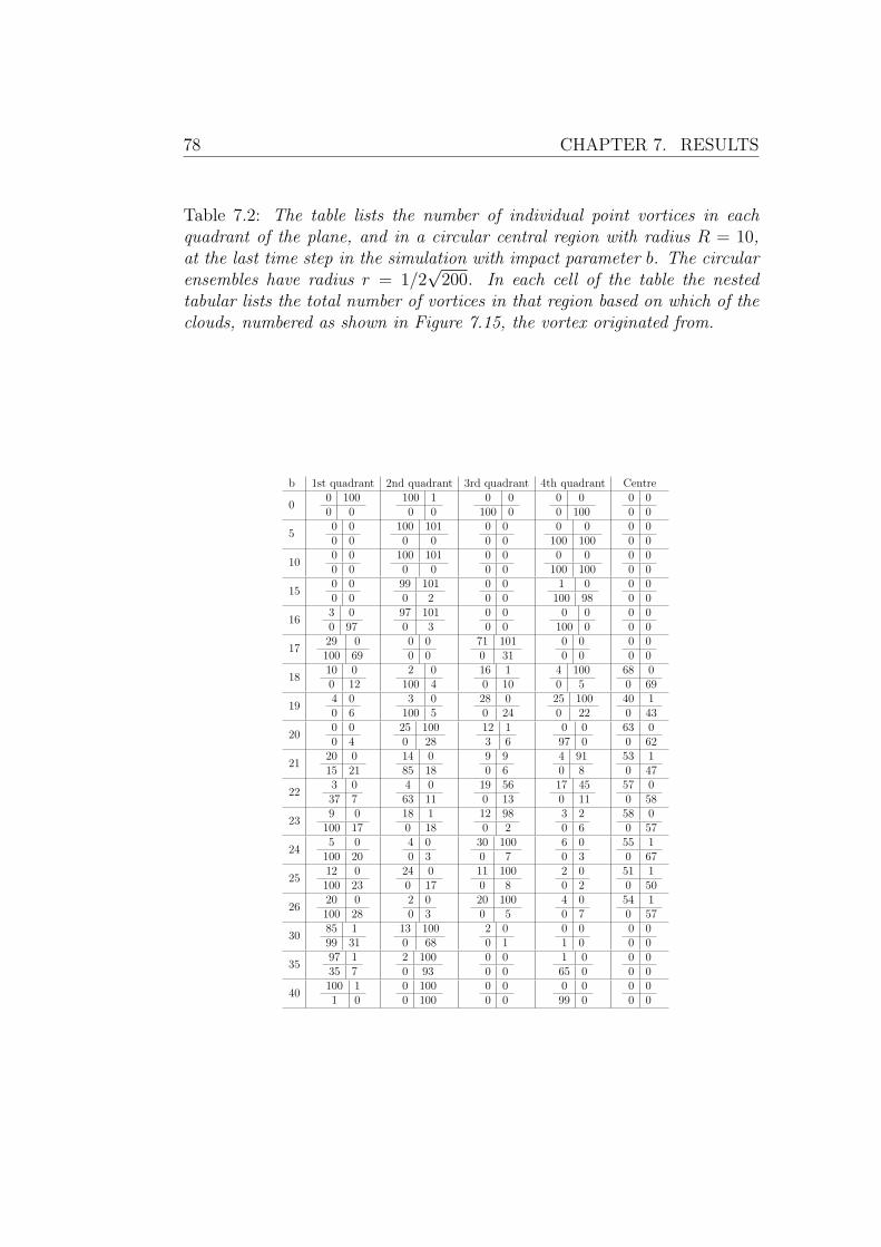
78 CHAPTER 7. RESULTS
Table 7.2: The table lists the number of individual point vortices in eachquadrant of the plane, and in a circular central region with radius R = 10,at the last time step in the simulation with impact parameter b. The circularensembles have radius r = 1/2
√200. In each cell of the table the nested
tabular lists the total number of vortices in that region based on which of theclouds, numbered as shown in Figure 7.15, the vortex originated from.
b 1st quadrant 2nd quadrant 3rd quadrant 4th quadrant Centre
00 1000 0
100 10 0
0 0100 0
0 00 100
0 00 0
50 00 0
100 1010 0
0 00 0
0 0100 100
0 00 0
100 00 0
100 1010 0
0 00 0
0 0100 100
0 00 0
150 00 0
99 1010 2
0 00 0
1 0100 98
0 00 0
163 00 97
97 1010 3
0 00 0
0 0100 0
0 00 0
1729 0100 69
0 00 0
71 1010 31
0 00 0
0 00 0
1810 00 12
2 0100 4
16 10 10
4 1000 5
68 00 69
194 00 6
3 0100 5
28 00 24
25 1000 22
40 10 43
200 00 4
25 1000 28
12 13 6
0 097 0
63 00 62
2120 015 21
14 085 18
9 90 6
4 910 8
53 10 47
223 037 7
4 063 11
19 560 13
17 450 11
57 00 58
239 0
100 1718 10 18
12 980 2
3 20 6
58 00 57
245 0
100 204 00 3
30 1000 7
6 00 3
55 10 67
2512 0100 23
24 00 17
11 1000 8
2 00 2
51 10 50
2620 0100 28
2 00 3
20 1000 5
4 00 7
54 10 57
3085 199 31
13 1000 68
2 00 1
0 01 0
0 00 0
3597 135 7
2 1000 93
0 00 0
1 065 0
0 00 0
40100 11 0
0 1000 100
0 00 0
0 099 0
0 00 0
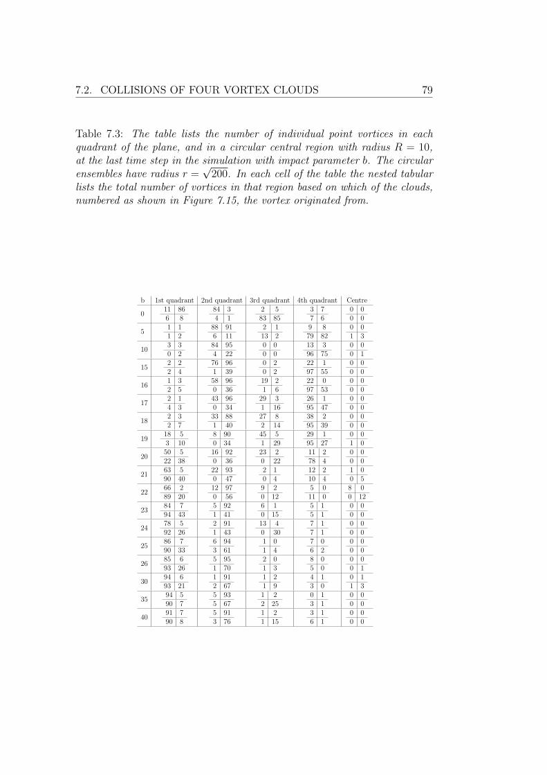
7.2. COLLISIONS OF FOUR VORTEX CLOUDS 79
Table 7.3: The table lists the number of individual point vortices in eachquadrant of the plane, and in a circular central region with radius R = 10,at the last time step in the simulation with impact parameter b. The circularensembles have radius r =
√200. In each cell of the table the nested tabular
lists the total number of vortices in that region based on which of the clouds,numbered as shown in Figure 7.15, the vortex originated from.
b 1st quadrant 2nd quadrant 3rd quadrant 4th quadrant Centre
011 866 8
84 34 1
2 583 85
3 77 6
0 00 0
51 11 2
88 916 11
2 113 2
9 879 82
0 01 3
103 30 2
84 954 22
0 00 0
13 396 75
0 00 1
152 22 4
76 961 39
0 20 2
22 197 55
0 00 0
161 32 5
58 960 36
19 21 6
22 097 53
0 00 0
172 14 3
43 960 34
29 31 16
26 195 47
0 00 0
182 32 7
33 881 40
27 82 14
38 295 39
0 00 0
1918 53 10
8 900 34
45 51 29
29 195 27
0 01 0
2050 522 38
16 920 36
23 20 22
11 278 4
0 00 0
2163 590 40
22 930 47
2 10 4
12 210 4
1 00 5
2266 289 20
12 970 56
9 20 12
5 011 0
8 00 12
2384 794 43
5 921 41
6 10 15
5 15 1
0 00 0
2478 592 26
2 911 43
13 40 30
7 17 1
0 00 0
2586 790 33
6 943 61
1 01 4
7 06 2
0 00 0
2685 693 26
5 951 70
2 01 3
8 05 0
0 00 1
3094 693 21
1 912 67
1 21 9
4 13 0
0 11 3
3594 590 7
5 935 67
1 22 25
0 13 1
0 00 0
4091 790 8
5 913 76
1 21 15
3 16 1
0 00 0
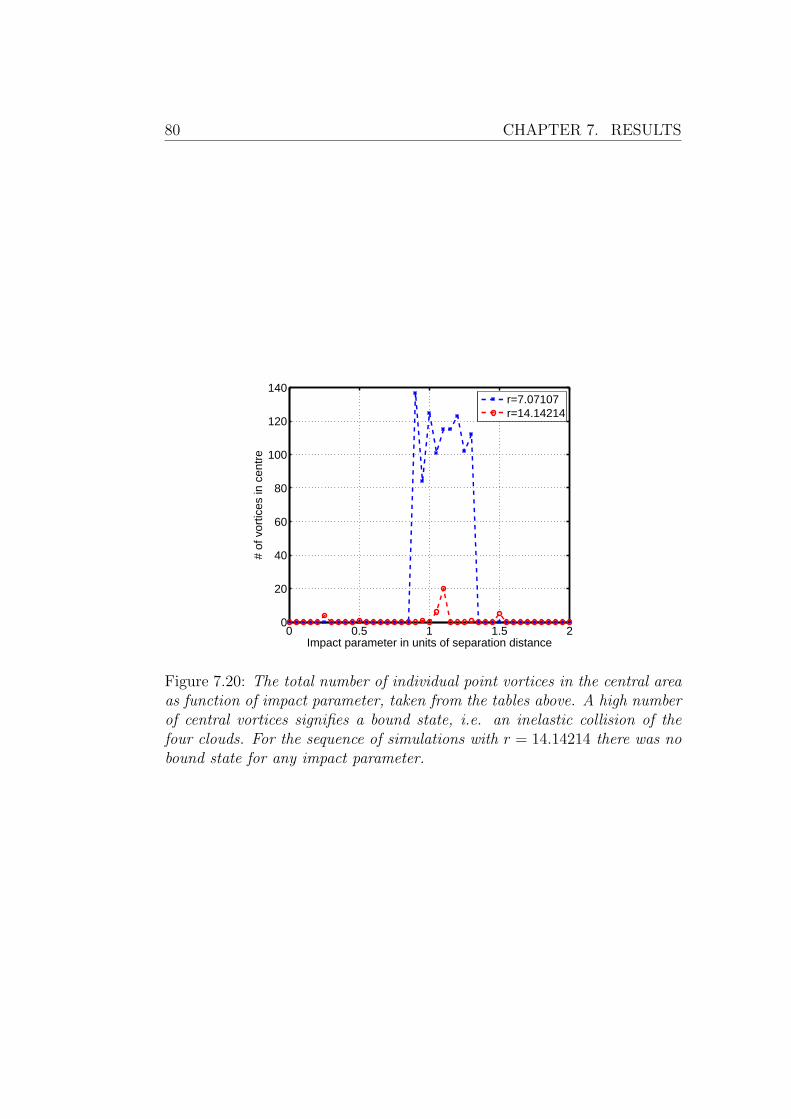
80 CHAPTER 7. RESULTS
0 0.5 1 1.5 20
20
40
60
80
100
120
140
Impact parameter in units of separation distance
# of
vor
tices
in c
entr
e
r=7.07107r=14.14214
Figure 7.20: The total number of individual point vortices in the central areaas function of impact parameter, taken from the tables above. A high numberof central vortices signifies a bound state, i.e. an inelastic collision of thefour clouds. For the sequence of simulations with r = 14.14214 there was nobound state for any impact parameter.
7.3. HOMOGENEOUS SYSTEMS 81
7.3 Homogeneous systems
For a description of the boundary conditions, see section 5.8
7.3.1 Constant vortex strengths
We have simulated a homogeneous system using periodic boundary condi-tions and image cells as an approximation. We did several simulations withthe same initial conditions with different random numbers used to gener-ate the initial uniform spatial distribution of vortices, where the position ofvortex i was (xi, yi), x, y ∈ (−10, 10). The total vorticity in all these sim-ulations was zero and P (γi = 0.1) = P (γi = −0.1) = 1/2 for vortex i. Thenumber of image cell layers was set to 4, see section 5.8, and the boundariesof the unit cell was the same as the initial spatial distribution. Also, thenumber of vortices simulated was Ns = 400 with Nt = Ne = Ns/10 = 40 testvortices and Eulerian points.
We ran one simulation with tmax = 100t0 and 13 with tmax = 30t0. Thesimulation time varied due to the different random numbers drawn in eachsimulation. If the numbers drawn were such that the velocities experiencedby the particles are high, the time step will be small, and the simulation willbe slow. In this, one vortex pair, separated by a particularly short distance,can dominate since the shortest separation distance and highest velocity areused to calculate the time step.
In all experiments we saved the velocity components of the test particlesand the components of the velocity field at the Eulerian points at every timestep. We used these as the raw data for statistical analysis.
The raw and analysed data from the single simulation with tmax = 100t0 isshown in Figures 7.21-7.30. Typical raw velocity data is shown in Figure 7.21.Figures 7.21(a) and 7.21(b) shows raw Lagrangian and Eulerian velocity data,respectively, of one vortex and fixed point for the entirety of the simulation.
The Lagrangian raw data shows a mean velocity close to zero, large vari-ations over time-scales of a few t0 with some sharp spikes, and many smallscale fluctuations. That the mean velocity is close to zero is as expectedfrom a fluctuating velocity field generated by an ensemble with net vorticityzero, and is consistent with the assumptions done in Chapter 4 on turbu-lent velocity fields. The large time scale variations in the velocity resultsfrom the overall interaction of the ensemble, sampled along the test vortextrajectory, while the small scale fluctuations are due to rapidly changing in-teractions between nearby vortices. The changes can be arbitrarily rapidsince the vortices are without inertia. If the velocity field changes, a vortexwill instantaneously adopt the new velocity.
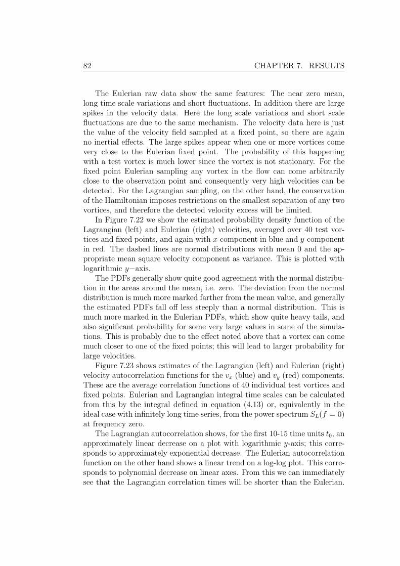
82 CHAPTER 7. RESULTS
The Eulerian raw data show the same features: The near zero mean,long time scale variations and short fluctuations. In addition there are largespikes in the velocity data. Here the long scale variations and short scalefluctuations are due to the same mechanism. The velocity data here is justthe value of the velocity field sampled at a fixed point, so there are againno inertial effects. The large spikes appear when one or more vortices comevery close to the Eulerian fixed point. The probability of this happeningwith a test vortex is much lower since the vortex is not stationary. For thefixed point Eulerian sampling any vortex in the flow can come arbitrarilyclose to the observation point and consequently very high velocities can bedetected. For the Lagrangian sampling, on the other hand, the conservationof the Hamiltonian imposes restrictions on the smallest separation of any twovortices, and therefore the detected velocity excess will be limited.
In Figure 7.22 we show the estimated probability density function of theLagrangian (left) and Eulerian (right) velocities, averaged over 40 test vor-tices and fixed points, and again with x-component in blue and y-componentin red. The dashed lines are normal distributions with mean 0 and the ap-propriate mean square velocity component as variance. This is plotted withlogarithmic y−axis.
The PDFs generally show quite good agreement with the normal distribu-tion in the areas around the mean, i.e. zero. The deviation from the normaldistribution is much more marked farther from the mean value, and generallythe estimated PDFs fall off less steeply than a normal distribution. This ismuch more marked in the Eulerian PDFs, which show quite heavy tails, andalso significant probability for some very large values in some of the simula-tions. This is probably due to the effect noted above that a vortex can comemuch closer to one of the fixed points; this will lead to larger probability forlarge velocities.
Figure 7.23 shows estimates of the Lagrangian (left) and Eulerian (right)velocity autocorrelation functions for the vx (blue) and vy (red) components.These are the average correlation functions of 40 individual test vortices andfixed points. Eulerian and Lagrangian integral time scales can be calculatedfrom this by the integral defined in equation (4.13) or, equivalently in theideal case with infinitely long time series, from the power spectrum SL(f = 0)at frequency zero.
The Lagrangian autocorrelation shows, for the first 10-15 time units t0, anapproximately linear decrease on a plot with logarithmic y-axis; this corre-sponds to approximately exponential decrease. The Eulerian autocorrelationfunction on the other hand shows a linear trend on a log-log plot. This corre-sponds to polynomial decrease on linear axes. From this we can immediatelysee that the Lagrangian correlation times will be shorter than the Eulerian.
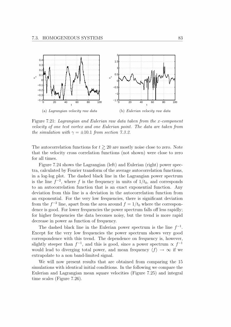
7.3. HOMOGENEOUS SYSTEMS 83
0 20 40 60 80 100−0.4
−0.3
−0.2
−0.1
0
0.1
0.2
0.3
0.4
t
v x
(a) Lagrangian velocity raw data
0 20 40 60 80 100−1.5
−1
−0.5
0
0.5
1
1.5
2
t
v x(b) Eulerian velocity raw data
Figure 7.21: Lagrangian and Eulerian raw data taken from the x-componentvelocity of one test vortex and one Eulerian point. The data are taken fromthe simulation with γ = ±10.1 from section 7.3.2.
The autocorrelation functions for t & 20 are mostly noise close to zero. Notethat the velocity cross correlation functions (not shown) were close to zerofor all times.
Figure 7.24 shows the Lagrangian (left) and Eulerian (right) power spec-tra, calculated by Fourier transform of the average autocorrelation functions,in a log-log plot. The dashed black line in the Lagrangian power spectrumis the line f−2, where f is the frequency in units of 1/t0, and correspondsto an autocorrelation function that is an exact exponential function. Anydeviation from this line is a deviation in the autocorrelation function froman exponential. For the very low frequencies, there is significant deviationfrom the f−2 line, apart from the area around f = 1/t0 where the correspon-dence is good. For lower frequencies the power spectrum falls off less rapidly;for higher frequencies the data becomes noisy, but the trend is more rapiddecrease in power as function of frequency.
The dashed black line in the Eulerian power spectrum is the line f−1.Except for the very low frequencies the power spectrum shows very goodcorrespondence with this trend. The dependence on frequency is, however,slightly steeper than f−1, and this is good, since a power spectrum ∝ f−1
would lead to diverging total power, and mean frequency 〈f〉 → ∞ if weextrapolate to a non band-limited signal.
We will now present results that are obtained from comparing the 15simulations with identical initial conditions. In the following we compare theEulerian and Lagrangian mean square velocities (Figure 7.25) and integraltime scales (Figure 7.26).
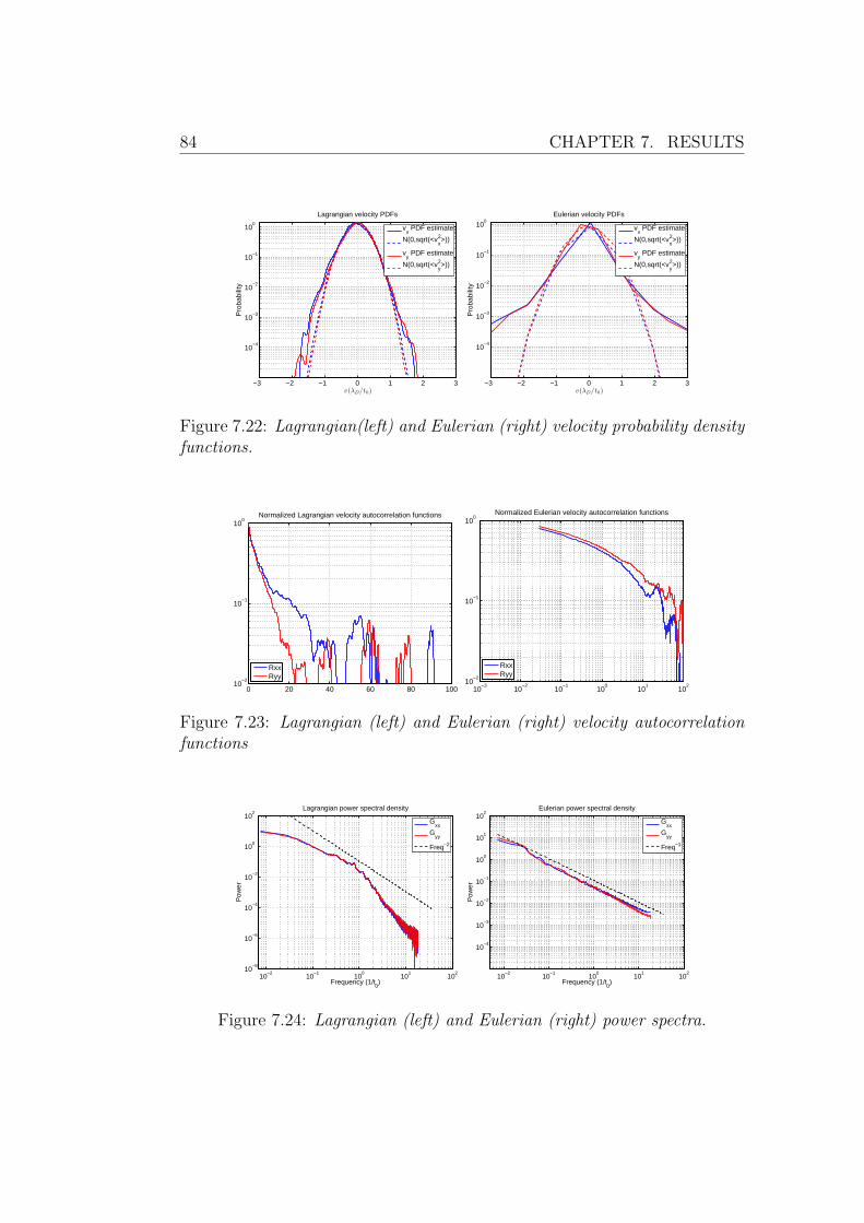
84 CHAPTER 7. RESULTS
−3 −2 −1 0 1 2 3
10−4
10−3
10−2
10−1
100
v(λD/t0)
Pro
babi
lity
Lagrangian velocity PDFs
vx PDF estimate
N(0,sqrt(<vx2>))
vy PDF estimate
N(0,sqrt(<vy2>))
−3 −2 −1 0 1 2 3
10−4
10−3
10−2
10−1
100
v(λD/t0)
Pro
babi
lity
Eulerian velocity PDFs
vx PDF estimate
N(0,sqrt(<vx2>))
vy PDF estimate
N(0,sqrt(<vy2>))
Figure 7.22: Lagrangian(left) and Eulerian (right) velocity probability densityfunctions.
0 20 40 60 80 10010
−2
10−1
100
Normalized Lagrangian velocity autocorrelation functions
RxxRyy
10−3
10−2
10−1
100
101
102
10−2
10−1
100
Normalized Eulerian velocity autocorrelation functions
RxxRyy
Figure 7.23: Lagrangian (left) and Eulerian (right) velocity autocorrelationfunctions
10−2
10−1
100
101
102
10−8
10−6
10−4
10−2
100
102
Frequency (1/t0)
Pow
er
Lagrangian power spectral density
Gxx
Gyy
Freq−2
10−2
10−1
100
101
102
10−4
10−3
10−2
10−1
100
101
102
Frequency (1/t0)
Pow
er
Eulerian power spectral density
Gxx
Gyy
Freq−1
Figure 7.24: Lagrangian (left) and Eulerian (right) power spectra.
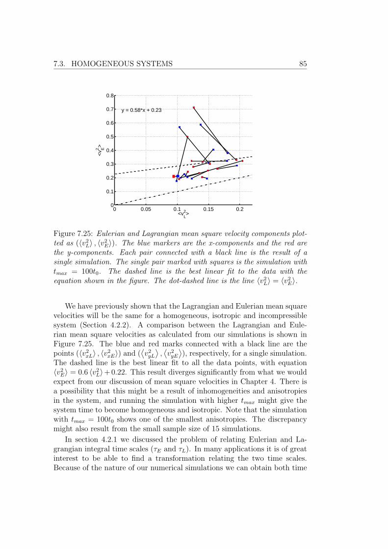
7.3. HOMOGENEOUS SYSTEMS 85
0 0.05 0.1 0.15 0.20
0.1
0.2
0.3
0.4
0.5
0.6
0.7
0.8
<vL2>
<v E2
>
y = 0.58*x + 0.23
Figure 7.25: Eulerian and Lagrangian mean square velocity components plot-ted as (〈v2
L〉 , 〈v2E〉). The blue markers are the x-components and the red are
the y-components. Each pair connected with a black line is the result of asingle simulation. The single pair marked with squares is the simulation withtmax = 100t0. The dashed line is the best linear fit to the data with theequation shown in the figure. The dot-dashed line is the line 〈v2
L〉 = 〈v2E〉.
We have previously shown that the Lagrangian and Eulerian mean squarevelocities will be the same for a homogeneous, isotropic and incompressiblesystem (Section 4.2.2). A comparison between the Lagrangian and Eule-rian mean square velocities as calculated from our simulations is shown inFigure 7.25. The blue and red marks connected with a black line are thepoints (〈v2
xL〉 , 〈v2xE〉) and (
⟨v2yL
⟩,⟨v2yE
⟩), respectively, for a single simulation.
The dashed line is the best linear fit to all the data points, with equation〈v2E〉 = 0.6 〈v2
L〉+ 0.22. This result diverges significantly from what we wouldexpect from our discussion of mean square velocities in Chapter 4. There isa possibility that this might be a result of inhomogeneities and anisotropiesin the system, and running the simulation with higher tmax might give thesystem time to become homogeneous and isotropic. Note that the simulationwith tmax = 100t0 shows one of the smallest anisotropies. The discrepancymight also result from the small sample size of 15 simulations.
In section 4.2.1 we discussed the problem of relating Eulerian and La-grangian integral time scales (τE and τL). In many applications it is of greatinterest to be able to find a transformation relating the two time scales.Because of the nature of our numerical simulations we can obtain both time
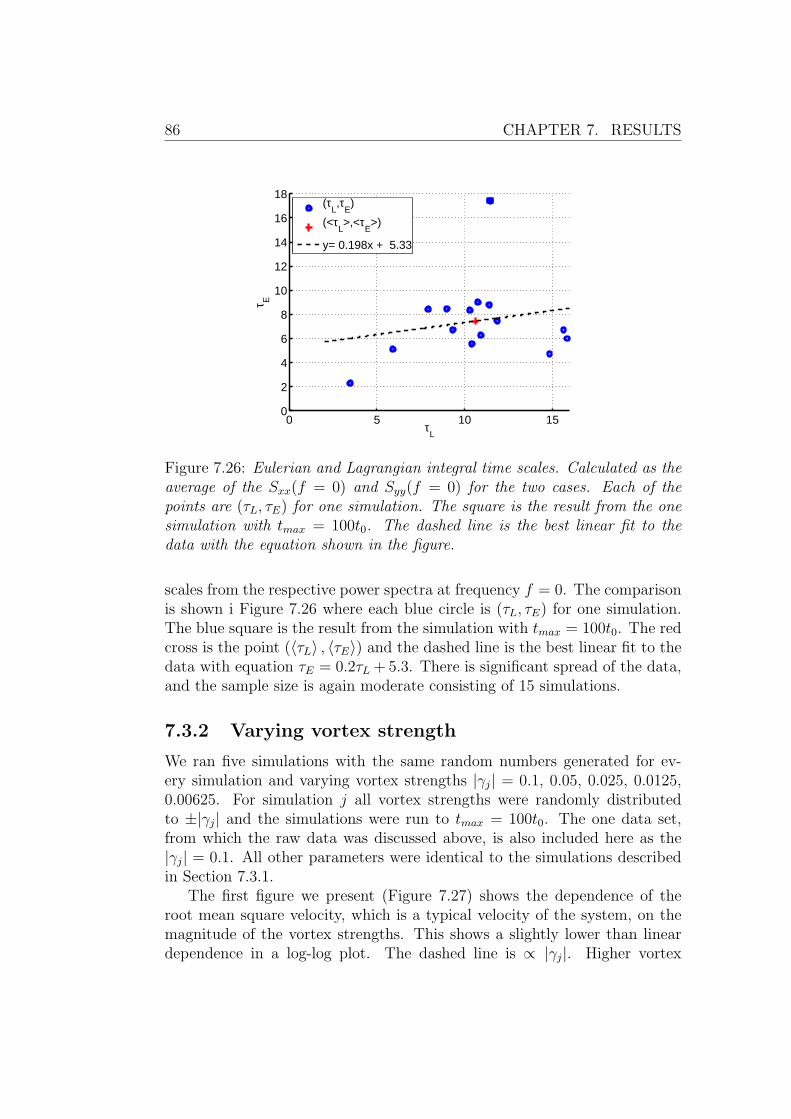
86 CHAPTER 7. RESULTS
0 5 10 150
2
4
6
8
10
12
14
16
18
τL
τ E
(τL,τ
E)
(<τL>,<τ
E>)
y= 0.198x + 5.33
Figure 7.26: Eulerian and Lagrangian integral time scales. Calculated as theaverage of the Sxx(f = 0) and Syy(f = 0) for the two cases. Each of thepoints are (τL, τE) for one simulation. The square is the result from the onesimulation with tmax = 100t0. The dashed line is the best linear fit to thedata with the equation shown in the figure.
scales from the respective power spectra at frequency f = 0. The comparisonis shown i Figure 7.26 where each blue circle is (τL, τE) for one simulation.The blue square is the result from the simulation with tmax = 100t0. The redcross is the point (〈τL〉 , 〈τE〉) and the dashed line is the best linear fit to thedata with equation τE = 0.2τL + 5.3. There is significant spread of the data,and the sample size is again moderate consisting of 15 simulations.
7.3.2 Varying vortex strength
We ran five simulations with the same random numbers generated for ev-ery simulation and varying vortex strengths |γj| = 0.1, 0.05, 0.025, 0.0125,0.00625. For simulation j all vortex strengths were randomly distributedto ±|γj| and the simulations were run to tmax = 100t0. The one data set,from which the raw data was discussed above, is also included here as the|γj| = 0.1. All other parameters were identical to the simulations describedin Section 7.3.1.
The first figure we present (Figure 7.27) shows the dependence of theroot mean square velocity, which is a typical velocity of the system, on themagnitude of the vortex strengths. This shows a slightly lower than lineardependence in a log-log plot. The dashed line is ∝ |γj|. Higher vortex
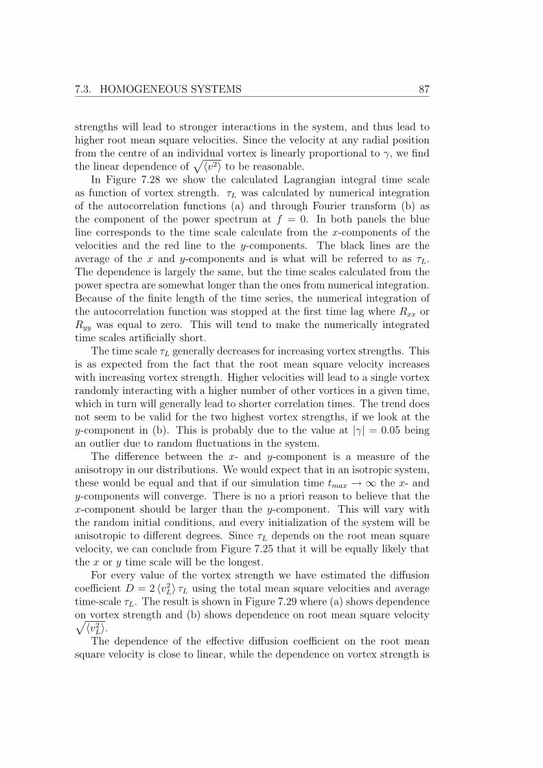
7.3. HOMOGENEOUS SYSTEMS 87
strengths will lead to stronger interactions in the system, and thus lead tohigher root mean square velocities. Since the velocity at any radial positionfrom the centre of an individual vortex is linearly proportional to γ, we findthe linear dependence of
√〈v2〉 to be reasonable.
In Figure 7.28 we show the calculated Lagrangian integral time scaleas function of vortex strength. τL was calculated by numerical integrationof the autocorrelation functions (a) and through Fourier transform (b) asthe component of the power spectrum at f = 0. In both panels the blueline corresponds to the time scale calculate from the x-components of thevelocities and the red line to the y-components. The black lines are theaverage of the x and y-components and is what will be referred to as τL.The dependence is largely the same, but the time scales calculated from thepower spectra are somewhat longer than the ones from numerical integration.Because of the finite length of the time series, the numerical integration ofthe autocorrelation function was stopped at the first time lag where Rxx orRyy was equal to zero. This will tend to make the numerically integratedtime scales artificially short.
The time scale τL generally decreases for increasing vortex strengths. Thisis as expected from the fact that the root mean square velocity increaseswith increasing vortex strength. Higher velocities will lead to a single vortexrandomly interacting with a higher number of other vortices in a given time,which in turn will generally lead to shorter correlation times. The trend doesnot seem to be valid for the two highest vortex strengths, if we look at they-component in (b). This is probably due to the value at |γ| = 0.05 beingan outlier due to random fluctuations in the system.
The difference between the x- and y-component is a measure of theanisotropy in our distributions. We would expect that in an isotropic system,these would be equal and that if our simulation time tmax → ∞ the x- andy-components will converge. There is no a priori reason to believe that thex-component should be larger than the y-component. This will vary withthe random initial conditions, and every initialization of the system will beanisotropic to different degrees. Since τL depends on the root mean squarevelocity, we can conclude from Figure 7.25 that it will be equally likely thatthe x or y time scale will be the longest.
For every value of the vortex strength we have estimated the diffusioncoefficient D = 2 〈v2
L〉 τL using the total mean square velocities and averagetime-scale τL. The result is shown in Figure 7.29 where (a) shows dependenceon vortex strength and (b) shows dependence on root mean square velocity√〈v2L〉.
The dependence of the effective diffusion coefficient on the root meansquare velocity is close to linear, while the dependence on vortex strength is
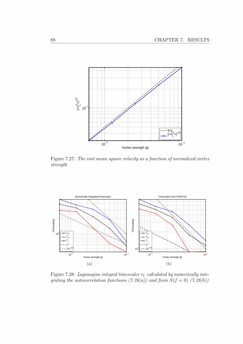
88 CHAPTER 7. RESULTS
10−2
10−1
10−1
Vortex strength (γ)
(<v L2 >
)1/2
5*γ(<v
L2>)1/2
Figure 7.27: The root mean square velocity as a function of normalized vortexstrength
10−2
10−1
101
Vortex strength (γ)
Tim
esca
le(γ
)
Numerically integrated timescales
τLx
τLy
τL
γ−1
2*γ−1/2
(a)
10−2
10−1
101
Vortex strength (γ)
Tim
esca
le(γ
)
Timescales from PSD(f=0)
τLx
τLy
τL
γ−1
2γ−1/2
(b)
Figure 7.28: Lagrangian integral timescales τL calculated by numerically inte-grating the autocorrelation functions (7.28(a)) and from S(f = 0) (7.28(b))
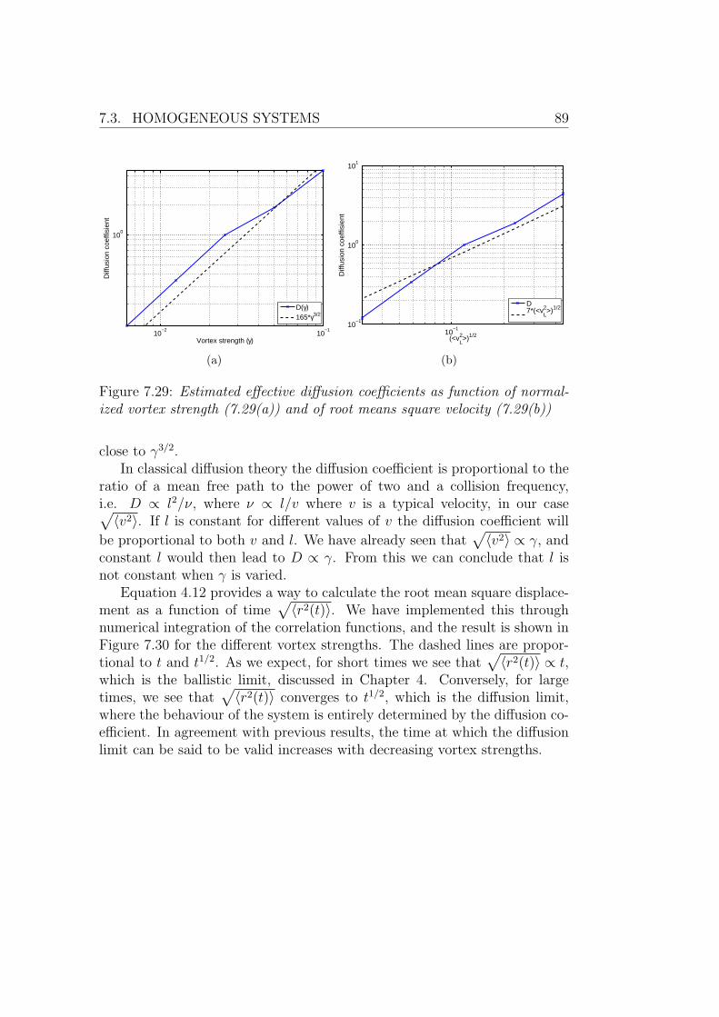
7.3. HOMOGENEOUS SYSTEMS 89
10−2
10−1
100
Vortex strength (γ)
Diff
usio
n co
effis
ient
D(γ)165*γ3/2
(a)
10−1
10−1
100
101
(<vL2>)1/2
Diff
usio
n co
effis
ient
D7*(<v
L2>)1/2
(b)
Figure 7.29: Estimated effective diffusion coefficients as function of normal-ized vortex strength (7.29(a)) and of root means square velocity (7.29(b))
close to γ3/2.In classical diffusion theory the diffusion coefficient is proportional to the
ratio of a mean free path to the power of two and a collision frequency,i.e. D ∝ l2/ν, where ν ∝ l/v where v is a typical velocity, in our case√〈v2〉. If l is constant for different values of v the diffusion coefficient will
be proportional to both v and l. We have already seen that√〈v2〉 ∝ γ, and
constant l would then lead to D ∝ γ. From this we can conclude that l isnot constant when γ is varied.
Equation 4.12 provides a way to calculate the root mean square displace-ment as a function of time
√〈r2(t)〉. We have implemented this through
numerical integration of the correlation functions, and the result is shown inFigure 7.30 for the different vortex strengths. The dashed lines are propor-tional to t and t1/2. As we expect, for short times we see that
√〈r2(t)〉 ∝ t,
which is the ballistic limit, discussed in Chapter 4. Conversely, for largetimes, we see that
√〈r2(t)〉 converges to t1/2, which is the diffusion limit,
where the behaviour of the system is entirely determined by the diffusion co-efficient. In agreement with previous results, the time at which the diffusionlimit can be said to be valid increases with decreasing vortex strengths.
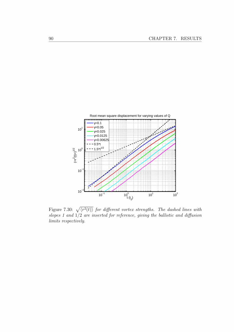
90 CHAPTER 7. RESULTS
10−1
100
101
102
10−2
10−1
100
101
t (t0)
(<r2 (t
)>)1/
2
Root mean square displacement for varying values of Q
γ=0.1γ=0.05γ=0.025γ=0.0125γ=0.006250.5*t
1.5*t1/2
Figure 7.30:√〈r2(t)〉 for different vortex strengths. The dashed lines with
slopes 1 and 1/2 are inserted for reference, giving the ballistic and diffusionlimits respectively.
Chapter 8
Discussions and Conclusions
Most of the results obtained have been discussed in the respective chaptersand sections. The present chapter will only give a summary.
We have demonstrated that a many vortex system can evolve to haveturbulence-like characteristics, such as turbulence-like correlation functions(Eulerian and Lagrangian) showing finite memory, continuous power spectra,etc. Also the basic features of turbulent transport are recovered. All this isfound for computationally moderate requirements, i.e. our models typicallycontain a few hundred to a few thousand discrete vortices. The model alsoallows studies of large-scale coherent structures obtained by superimposingmany discrete vortices. The present model is found to have randomly varyingvelocity fields as in turbulent neutral flows. One important difference is thatclassical turbulence is generally seen as a driven-dissipative system. For thepresent vortex system the Hamiltonian is given by the initial conditions andenergy is neither dissipated nor injected.
We have analysed and demonstrated a number of basic properties of vor-tex systems and their numerical implementation.
1. In the implementation of the numerical model there were some areasof special concern:
Variable time step: To ensure that a vortex system is simulatedcorrectly, careful attention must be paid to the time step usedwhen solving the differential equations. We came to the conclusionthat a variable time step, calculated in every iteration was themost efficient way to ensure adequate time resolution.
Periodic boundary conditions and image cells: The correct imple-mentation of periodic boundary conditions and the handling ofinteractions with vortices in image cells presented a major chal-lenge
91
92 CHAPTER 8. DISCUSSIONS AND CONCLUSIONS
Subroutines for Bessel functions: The efficiency of any Besselfunction subroutine is of great importance for large simulations.Highly optimized routines for calculating the modified Bessel func-tions should be a focus if large simulations of shielded vortices areof interest.
2. The basic properties of low dimensional vortex systems have been re-covered through numerical simulations. We have demonstrated:
The propagation of vortex pairs for different combinations of vor-tex strengths.
Vortex pair collisions for different impact parameters.
The expansion/collapse of a vortex triplet given specific initialconditions.
3. We have studied the time evolution of large-scale coherent structuresby superimposing many discrete vortices.
A vortex cloud of one polarity will have a long life time as acoherent structure. This is also valid for a pair of vortex cloudsof opposite polarities.
A vortex cloud of approximately zero vorticity density will haveshort life time as a coherent structure.
Collisions of two vortex cloud pairs display the same basic dynam-ics as vortex pair collisions for small impact parameters. Estab-lished also parameter range for inelastic collisions.
4. The basic features of turbulent transport are recovered in terms of anapproximately homogeneous and isotropic system of point vortices.
Realized the evolution of turbulent spectra for the velocity field.
Established phenomenological relations between Eulerian and La-grangian integral time scales.
Identified ballistic and diffusive limits for turbulent diffusion ofsingle particles.
8.1 Future perspectives
The time one has for the completion of a masters degree is necessarily limited.Due to this, many goals and interesting projects could not be completed. If
8.1. FUTURE PERSPECTIVES 93
we get the opportunity to continue this study at a later time, the followingchanges and refinements would be prioritized:
The implementation of Ewald summation methods for calculating theinteractions in the periodic system. This will allow for a greater numberof image cells without increasing the simulation time.
The reformulation of the model by the use of “vortex-in-cell” methods(Leonard, 1980), similar to particle-in-cell methods. This will allow fora larger number of simulated vortices.
The consideration of other vortex interaction functions F than the log-arithmic an Bessel function interactions covered in this thesis. Thevortices considered in this study are all singular for r = 0, other inter-action functions can have the advantage of removing this singularity.
The implementation of vortices of finite size.
Incorporation of polarization drifts, i.e. the first higher order correctionin the parameter 〈ω〉 /Ωc. This will be a very challenging problemanalytically, and it has never been approached for vortex systems. (Formodel equations based on fluid theory this problem is much easier.)

94 CHAPTER 8. DISCUSSIONS AND CONCLUSIONS
Bibliography
M. Abramowitz and I. A. Stegun. Handbook of Mathematical Functions.Dover Publications, New York, 1965.
H. Aref. Motion of three vortices. Physics of Fluids, 22(3):393–400, 1979.
H. Aref. Integrable, chaotic and turbulent vortex motion in two-dimensionalflows. Annual Review of Fluid Mechanics, 15:345–389, 1983.
G. K. Batchelor. Diffusion in a field of homogeneous turbulence. Aust. J.Sci. Res., 2:437–450, 1949.
S. Corrsin. Estimates of the relations between eulerian and lagrangian scalesin large reynolds number turbulence. Journal of the Atmospheric Sciences,20(2):115–119, 1963.
William Crookes. The bakerian lecture: On the illumination of lines of molec-ular pressure, and the trajectory of molecules. Philosophical Transactionsof the Royal Society of London, 170:135–164.
U. Frisch. Turbulence: The Legacy of A. N. Kolmogorov. Cambridge Uni-versity Press, 1996.
W. Horton. Drift waves and transport. Rev. Mod. Phys., 71:735–778, Apr1999.
Y. Kimura. Similarity Solution of Two-Dimensional Point Vortices. Journalof the Physical Society of Japan, 56(6):2024–2030, 1987.
M. Kono, B. Krane, H. L. Pecseli, and J. Trulsen. Vortex dynamics inmagnetized plasmas. Phys. Scripta, 58:238–245, 1998.
I Langmuir. Oscillations in ionized gases. Proceedings of the NationalAcademy of Sciences of The United States of America, 14:627–637, 1928.
95
96 BIBLIOGRAPHY
A Leonard. Vortex Methods for Flow Simulation. Journal of ComputationalPhysics, 37(3):289–335, 1980.
P. C. Liewer. Measurements of Microturbulence in Tokamaks and Com-parisons with Theories of Turbulence and Anomalous Transport. NuclearFusion, 25(5):543–621, 1985.
J. L. Lumley. Approach to Eulerian-Lagrangian Problem. Journal of Math-ematical Physics, 3(2):309–&, 1962.
J. L. Lumley and H. A. Panofsky. The Sructure of Atmospheric turbulence.Interscience Publishers, 1964.
J. P. Lynov, A. H. Nielsen, H. L. Pecseli, and J. J. Rasmussen. Studies ofthe Eulerian-Lagrangian transformation in 2-dimansional random flows.Journal of Fluid Mechanics, 224:485–505, 1991.
M. Marvan. Negative Absolute Temperatures. Number 4 in Physics Paper-backs. Iliffe, London, 1966.
G. K. Morikawa and E. V. Swenson. Interacting Motion of RectilinearGeostrophic Vortices. Physics of Fluids, 14(6):1058–1073, 1971.
A. Okamoto, K. Hara, K. Nagaoka, S. Yoshimura, J. Vranjes, M Kono, andM. Y. Tanaka. Experimental observation of a tripolar vortex in a plasma.Physics of Plasmas, 10(6):2211–2216, 2003.
A. Okamoto, K. Nagaoka, S. Yoshimura, J. Vranjes, S. Kado, M Kono, andM. Y. Tanaka. Tripolar vortex in a plasma. IEEE Transactions on PlasmaSciences, 33(2, Part 1):452–453, 2005.
R. K. Pathria. Statistical Mechanics. Butterworth-Heinemann, Oxford, 2edition, 1998.
H. Poincare. Theorie des Tourbillons. Editions Jacques Gabay, Paris, 1893.
H. L. Pecseli. Fluctuations in Physical Systems. Cambridge University Press,2000.
P. H. Roberts. On the application of a statistical approximation to the theoryof turbulent diffusion. J. Math. and Mech., 6:781–799, 1957.
Yu. B. Rumer and M. Sh. Ryvkin. Thermodynamics, Statistical Physics andKinetics. MIR Publishers, 1980.

BIBLIOGRAPHY 97
H. Tennekes and J. L. Lumley. A First Course in Turbulence. The MITpress, Cambridge, Massachusetts, 1972.
J. Vranjes, A. Okamoto, S. Yoshimura, S. Poedts, M. Kono, and M. Y.Tanaka. Analytical description of a neutral-induced tripole vortex in aplasma. Physical Review Letters, 89(26), DEC 23 2002.

98 BIBLIOGRAPHY
Appendix A
C++ source code
99
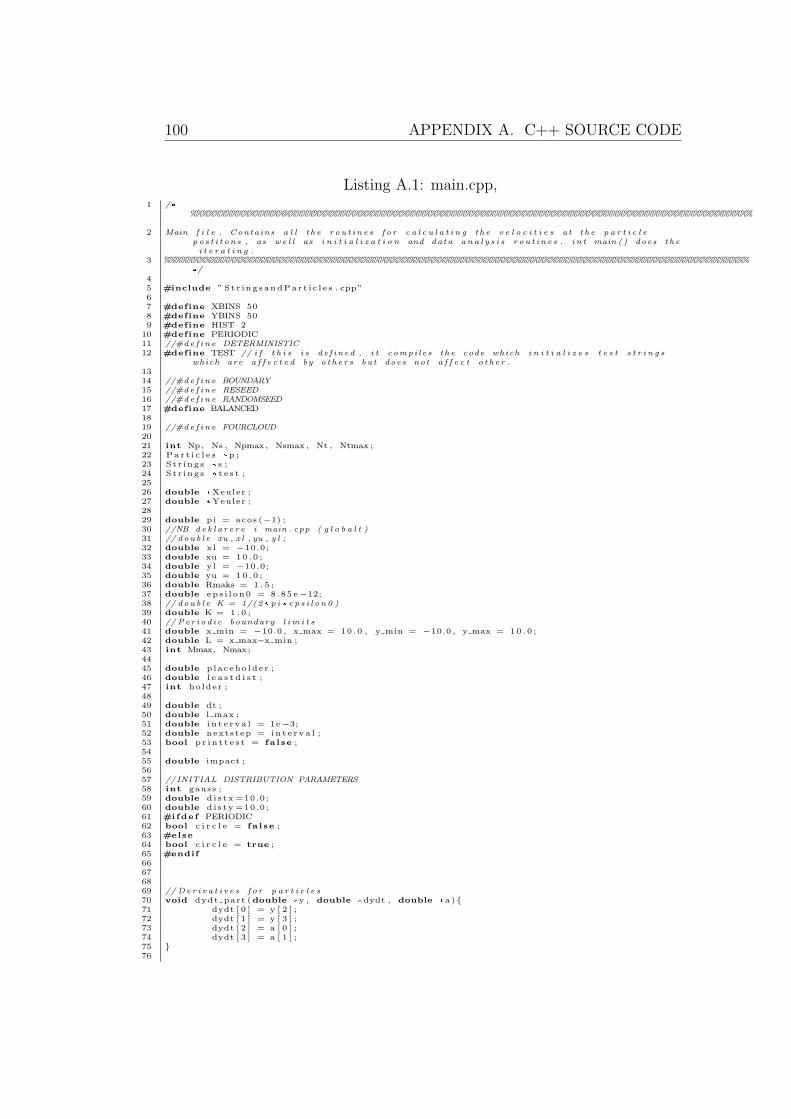
100 APPENDIX A. C++ SOURCE CODE
Listing A.1: main.cpp,1 /*
%%%%%%%%%%%%%%%%%%%%%%%%%%%%%%%%%%%%%%%%%%%%%%%%%%%%%%%%%%%%%%%%%%%%%%%%%%%%%%%%%%%%%%%%%%%%%%%%
2 Main f i l e . Contains a l l t h e r o u t i n e s f o r c a l c u l a t i n g t h e v e l o c i t i e s a t t h e p a r t i c l ep o s t i t o n s , as w e l l as i n i t i a l i z a t i o n and data a n a l y s i s r o u t i n e s . i n t main ( ) does t h ei t e r a t i n g .
3 %%%%%%%%%%%%%%%%%%%%%%%%%%%%%%%%%%%%%%%%%%%%%%%%%%%%%%%%%%%%%%%%%%%%%%%%%%%%%%%%%%%%%%%%%%%%%%%%%%%%*/
45 #include ” S t r i n g s andPa r t i c l e s . cpp”67 #define XBINS 508 #define YBINS 509 #define HIST 2
10 #define PERIODIC11 //#d e f i n e DETERMINISTIC12 #define TEST // i f t h i s i s de f ined , i t c omp i l e s t h e code which i n i t i a l i z e s t e s t s t r i n g s
which are a f f e c t e d by o t h e r s bu t does not a f f e c t o t h e r .1314 //#d e f i n e BOUNDARY15 //#d e f i n e RESEED16 //#d e f i n e RANDOMSEED17 #define BALANCED1819 //#d e f i n e FOURCLOUD2021 int Np, Ns , Npmax, Nsmax , Nt , Ntmax ;22 Pa r t i c l e s *p ;23 S t r i ng s * s ;24 S t r i ng s * t e s t ;2526 double *Xeuler ;27 double *Yeuler ;2829 double pi = acos (−1) ;30 //NB d e k l a r e r e i main . cpp ( g l o b a l t )31 // doub l e xu , x l , yu , y l ;32 double x l = −10.0;33 double xu = 10 . 0 ;34 double y l = −10.0;35 double yu = 10 . 0 ;36 double Rmaks = 1 . 5 ;37 double ep s i l on0 = 8.85 e−12;38 // doub l e K = 1/(2* p i* e p s i l o n 0 )39 double K = 1 . 0 ;40 // Pe r i o d i c boundary l i m i t s41 double x min = −10.0 , x max = 10 .0 , y min = −10.0 , y max = 10 . 0 ;42 double L = x max−x min ;43 int Mmax, Nmax;4445 double p lac eho lde r ;46 double l e a s t d i s t ;47 int ho lder ;4849 double dt ;50 double l max ;51 double i n t e r v a l = 1e−3;52 double nextstep = i n t e r v a l ;53 bool p r i n t t e s t = fa l se ;5455 double impact ;5657 //INITIAL DISTRIBUTION PARAMETERS58 int gauss ;59 double d i s t x =10.0;60 double d i s t y =10.0;61 #ifde f PERIODIC62 bool c i r c l e = fa l se ;63 #else64 bool c i r c l e = true ;65 #endif66676869 // De r i v a t i v e s f o r p a r t i c l e s70 void dydt part (double *y , double *dydt , double *a )71 dydt [ 0 ] = y [ 2 ] ;72 dydt [ 1 ] = y [ 3 ] ;73 dydt [ 2 ] = a [ 0 ] ;74 dydt [ 3 ] = a [ 1 ] ;75 76
101
77 // De r i v a t i v e s f o r s t r i n g s78 void dydt s t r i ng (double *y , double *dydt , double *v )79 dydt [ 0 ] = v [ 0 ] ;80 dydt [ 1 ] = v [ 1 ] ;81 8283 // I n i t i a l i z e s t h e s t r i n g s and p a r t i c l e s w i th a f i l e name and a l l v a l u e s s e t t o 0 .84 //Uses t h e c on s t r u c t o r in c l a s s s t r i n g s a n d p a r t i c l e s85 void i n i t i a l i z e (double T, double dt )8687 Ns = Np = Nt = 0 ;88 i f (Npmax>0) p= new Pa r t i c l e s [Npmax ] ;89 i f (Nsmax>0) s= new St r i ng s [Nsmax ] ;90 #ifde f TEST91 i f (Ntmax>0) t e s t = new St r i ng s [Ntmax ] ;92 #endif93 double Q=0. , B=0. ;94 double q=0.0 , m=0. ,u=0. ,v=0. ,x=0. ,y=0. ; //Charge , mass9596 s t r i n g header=”” ;97 #ifde f PSPRINT98 header=”header .m” ;99 ofstream mf i l ;
100 mf i l . open ( header . c s t r ( ) , i o s : : trunc ) ;101 mfi l<<”Np=”<<Npmax<<” ; ”<<endl102 <<”Ns=”<<Nsmax<<” ; ”<<endl ;103104 mf i l . c l o s e ( ) ;105 #endif106107 for ( int i =0; i<Nsmax;++ i )108 s [ i ] . i n i t i a l i z e ( header , i , x , y ,Q,B, dt , dyd t s t r i ng ) ;109 110 for ( int i =0; i<Npmax;++ i )111 p [ i ] . i n i t i a l i z e ( header , i , x , y , u , v , q ,m, dt , dydt part ) ;112 113 #ifde f TEST114 for ( int i =0; i<Ntmax;++ i )115 t e s t [ i ] . i n i t i a l i z e ( header , i , x , y ,Q,B, dt , dyd t s t r i ng ) ;116 117 #endif118119 120121 // Generates t h e s t r i n g s and p a r t i c l e s by making a a r b i t r a r y number o f t h e a c t i v e and
f i x i n g t h e i r v a l u e s122 void generate ( int Npgen , int Nsgen , int Ntgen , bool i n i t i a l )123 // I n i t i a l i z e random func t i on , dump f i r s t v a l u e124 #i f d e f RANDOMSEED125 srand48 ( int ( time (NULL) ) ) ; drand48 ( ) ;126 #else127 srand48 (1) ; drand48 ( ) ;128 #end i f129 double Q=1. , B=1. ;130 double q=0.0 , m=1. ; //Charge , mass131 double x , y , u , v ;132 double Q ef f =0.0 , Q e f f2 = 0 . 0 ;133134135 i f (Nsgen+Ns<=Nsmax)136137 #ifde f FOURCLOUD138 for ( int i =0; i<Nsgen / 4 . 0 ; ++i )139 i f ( i n i t i a l )140 double rad , angle , semi1 , semi2 ;141 semi1 =1.0; semi2 =1.0;142 rad = 0.1* sq r t ( d i s t x * d i s t x+d i s t y * d i s t y ) * sq r t ( drand48 ( ) ) ;143 angle = 2* pi *drand48 ( ) ;144 x = 20+semi1* rad* cos ( ang le ) ;145 y = impact+10+semi2* rad* s i n ( angle ) ;146147 else148 x=0.0;149 y=0.0;150 151 Q=drand48 ( ) ;152 while (Q==0.0)Q=drand48 ( ) ;153 i f (Q<0.0)Q = 1 ;154 else i f (Q>0.0) Q = 1 ;155 else cout<<”DAFUQ”<<” Q=”<<Q<<endl ;156157 s [ Ns++]. s e t a l l (x , y ,Q,B) ;158
102 APPENDIX A. C++ SOURCE CODE
159 for ( int i=Nsgen / 4 . 0 ; i<Nsgen / 2 . 0 ; ++i )160 i f ( i n i t i a l )161 double rad , angle , semi1 , semi2 ;162 semi1 =1.0; semi2 =1.0;163 rad = 0.1* sq r t ( d i s t x * d i s t x+d i s t y * d i s t y ) * sq r t ( drand48 ( ) ) ;164 angle = 2* pi *drand48 ( ) ;165 x = −20+semi1* rad* cos ( ang le ) ;166 y = 10+semi2* rad* s i n ( angle ) ;167168 else169 x=0.0;170 y=0.0;171 172 Q=drand48 ( ) ;173 while (Q==0.0)Q=drand48 ( ) ;174 i f (Q<0.0)Q = −1;175 else i f (Q>0.0) Q = −1;176 else cout<<”DAFUQ”<<” Q=”<<Q<<endl ;177178 s [ Ns++]. s e t a l l (x , y ,Q,B) ;179 180 for ( int i=Nsgen / 2 . 0 ; i<3*Nsgen /4 ; ++i )181 i f ( i n i t i a l )182 double rad , angle , semi1 , semi2 ;183 semi1 =1.0; semi2 =1.0;184 rad = 0.1* sq r t ( d i s t x * d i s t x+d i s t y * d i s t y ) * sq r t ( drand48 ( ) ) ;185 angle = 2* pi *drand48 ( ) ;186 x = −20+semi1* rad* cos ( ang le ) ;187 y = −10+semi2* rad* s i n ( angle ) ;188189 else190 x=0.0;191 y=0.0;192 193 Q=drand48 ( ) ;194 while (Q==0.0)Q=drand48 ( ) ;195 i f (Q<0.0)Q = 1 ;196 else i f (Q>0.0) Q = 1 ;197 else cout<<”DAFUQ”<<” Q=”<<Q<<endl ;198199 s [ Ns++]. s e t a l l (x , y ,Q,B) ;200 201 for ( int i =3*Nsgen / 4 . 0 ; i<Nsgen ; ++i )202 i f ( i n i t i a l )203 double rad , angle , semi1 , semi2 ;204 semi1 =1.0; semi2 =1.0;205 rad = 0.1* sq r t ( d i s t x * d i s t x+d i s t y * d i s t y ) * sq r t ( drand48 ( ) ) ;206 angle = 2* pi *drand48 ( ) ;207 x = 20+semi1* rad* cos ( ang le ) ;208 y = impact−10+semi2* rad* s i n ( angle ) ;209210 else211 x=0.0;212 y=0.0;213 214 Q=drand48 ( ) ;215 while (Q==0.0)Q=drand48 ( ) ;216 i f (Q<0.0)Q = −1;217 else i f (Q>0.0) Q = −1;218 else cout<<”DAFUQ”<<” Q=”<<Q<<endl ;219220 s [ Ns++]. s e t a l l (x , y ,Q,B) ;221 222 #else //
************************************************************************************************
223 for ( int i =0; i<Nsgen ; ++i )224 i f ( i n i t i a l )225 i f ( c i r c l e )226 double rad , angle , semi1 , semi2 ;227 semi1 =2.0; semi2 =0.5;228 rad = sqr t ( d i s t x * d i s t x+d i s t y * d i s t y ) * sq r t ( drand48
( ) ) ;229 angle = 2* pi *drand48 ( ) ;230 x = semi1* rad* cos ( ang le ) ;231 y = semi2* rad* s i n ( angle ) ;232 else 233 x=2*d i s t x *drand48 ( )−d i s t x ;234 y=2*d i s t y *drand48 ( )−d i s t y ;235 cout<<y<<endl ;236 237 238 else
103
239 x=0.0; // E l l e r x=drand48 ( )*vx240 y=0.0;241 242 i f ( gauss==1)243 double Ran1 , Ran2 , Ran3 ;244 Ran1 = drand48 ( ) ;245 Ran2 = drand48 ( ) ;246 cout<<Ran1<<” ”<<Ran2<<endl ;247 Ran3 = sqr t (−2* l og (Ran1) ) * cos (2* pi *Ran2) ;248 Q = 1 .0/2 . 0*Ran3 ;249 // cout<<Q<<end l ;250 while (Q==0.0)251 Ran1 = drand48 ( ) ;252 Ran2 = drand48 ( ) ;253 cout<<” In s i d e loop : ”<<Ran1<<” ”<<Ran2<<endl ;254 Ran3 = sqr t (−2* l og (Ran1) ) * cos (2* pi *Ran2) ;255 cout<<” In s i d e loop Ran3=:”<<Ran3<<endl ;256 Q = 1 .0/2 . 0*Ran3 ;257 // cout<<Q<<end l ;258 259 else i f ( gauss==0)260 Q=2.0*drand48 ( ) −1.0;261 while (Q==0.0)Q=drand48 ( ) ;262 i f (Q<0.0)Q = −1.0;263 else i f (Q>0.0) Q = 1 . 0 ;264 else cout<<”DAFUQ”<<” Q=”<<Q<<endl ;265 Q e f f += Q;266 // cout<<”Q e f f=”<<Q ef f<<end l ;267 #i f d e f BALANCED268 i f ( i<Nsgen /2) Q = 1 . 0 ;269 else Q = −1.0;270 Q e f f2 += Q;271 // cout<<”Q e f f 2=”<<Q ef f2<<end l ;272 #end i f273 else i f ( gauss==2)274 Q=2.0*drand48 ( ) −1.0;275 while (Q==0.0)Q=2.0*drand48 ( ) −1.0;276 else cout<<” gauss=”<<gauss<<endl ;277 Q /= 10 . 0 ;278 s [ Ns++]. s e t a l l (x , y ,Q,B) ;279 280281 else cout<<” could not generate ”<<endl ;282 i f (Npgen+Np<=Npmax)283 for ( int i =0; i<Npgen ; ++i )284 x=drand48 ( ) ;285 y=drand48 ( ) ;286 u=drand48 ( ) ;287 v=drand48 ( ) ;288 p [Np++]. s e t a l l (x , y , u , v , q ,m) ;289 290291 #endif292 cout<<”Ns=”<<Ns<<” ”<<”Np=”<<Np<<endl ;293 #ifde f TEST294 for ( int i =0; i<Ntgen;++ i )295 x = 2* d i s t x *drand48 ( )−d i s t x ;296 y = 2* d i s t y *drand48 ( )−d i s t y ;297 i f ( gauss==1)298 double Ran1 , Ran2 , Ran3 ;299 Ran1 = drand48 ( ) ;300 Ran2 = drand48 ( ) ;301 cout<<Ran1<<” ”<<Ran2<<endl ;302 Ran3 = sqr t (−2* l og (Ran1) ) * cos (2* pi *Ran2) ;303 Q = 1 .0/2 . 0*Ran3 ;304 // cout<<Q<<end l ;305 while (Q==0.0)306 Ran1 = drand48 ( ) ;307 Ran2 = drand48 ( ) ;308 cout<<” In s i d e loop : ”<<Ran1<<” ”<<Ran2<<endl ;309 Ran3 = sqr t (−2* l og (Ran1) ) * cos (2* pi *Ran2) ;310 cout<<” In s i d e loop Ran3=:”<<Ran3<<endl ;311 Q = 1 .0/2 . 0*Ran3 ;312 // cout<<Q<<end l ;313 314 else i f ( gauss==0)315 Q=2.0*drand48 ( ) −1.0;316 while (Q==0.0)Q=drand48 ( ) ;317 i f (Q<0.0)Q = −1.0;318 else i f (Q>0.0) Q = 1 . 0 ;319 else cout<<”DAFUQ”<<” Q=”<<Q<<endl ;320 // cout<<”Q=”<<Q<<end l ;321 else i f ( gauss==2)
104 APPENDIX A. C++ SOURCE CODE
322 Q=2.0*drand48 ( ) −1.0;323 while (Q==0.0)Q=2.0*drand48 ( ) −1.0;324 else cout<<” gauss=”<<gauss<<endl ;325 t e s t [ Nt++]. s e t a l l (x , y ,Q,B) ;326327 328329 #endif330 // cout<<”Q e f f=”<<Q ef f<<” Q e f f 2=”<<Q ef f2<<end l ;331 // cin>>Q e f f ;332 333334335 // Ca l c u l a t e s t h e f o r c e on a p a r i c l e in t h e f i e l d g ene ra t ed by a l l o t h e r s t r i n g s and
p a r t i c l e s336 void movepar t i c l e s ( int Mmax, int Nmax)337 double Fqx , Fqy , x , y , u , v ;338 double Ex=0.0 , Ey=0.0 , B=0.0 , Etx , Ety , Bt ;339 int nbox , mbox ;340 // cout<<”mov e p a r t i c l e s”<<end l ;341 for ( int i =0; i<Np; ++i )342 Ex=Ey=B=0.0;343 Etx=Ety=Bt=0.0;344 // cout<<”main : : mo v e p a r t i c l e s : i=”<<i<< end l ;345 Etx=Ety=Bt=0.0; //Temp v a r i a b l e s346 p [ i ] . g e tpo sve l (&x,&y,&u,&v) ;347 for (mbox=−Mmax;mbox<=Mmax;++mbox)348 for ( nbox=−Nmax; nbox<=Nmax;++nbox )349 for ( int j =0; j<i ; ++j )350 // cout<<”mov e p a r t i c l e s ( l ower ) j=”<<j<<end l ;351 p [ j ] . getE (x , y,&Etx ,&Ety ,mbox , nbox ,L) ;352 Ex+=Etx , Ey+=Ety ;353 // cout<<”lower : Ex=”<<Ex<<” Ey=”<<Ey<<end l ;354 355 for ( int j=i +1; j<Np; ++j )356 // cout<<”mov e p a r t i c l e s ( h i g h e r ) j=”<<j<<end l ;357 p [ j ] . getE (x , y,&Etx ,&Ety ,mbox , nbox ,L) ;358 Ex+=Etx , Ey+=Ety ;359 // cout<<”h i g h e r : Ex=”<<Ex<<” Ey=”<<Ey<<end l ;360 361 for ( int j =0; j<Ns ; ++j )362 // cout<<”mov e p a r t i c l e s ( s t r i n g s ) j=”<<j<<end l ;363 s [ j ] . getEB (x , y,&Etx ,&Ety ,&Bt ,mbox , nbox ,L , &
p lac eho lde r ) ;364 Ex+=Etx , Ey+=Ety , B+=Bt ;365 // cout<<”s t r i n g s : Ex=”<<Ex<<” Ey=”<<Ey<<” B=”<<B
<<end l ;366 367 368 369 B = B/Ns ;370 // cout<<”B=”<<B<<end l ;371 // Ca l c u l a t e F/q372 Fqx = K*Ex + v*B;373 Fqy = K*Ey − u*B;374375 //Pass f o r c e / charge to p a r t i c l e i376 p [ i ] . setFq (Fqx , Fqy) ;377 // cout<<end l ;378 379 380381 // Ca l c u l a t e s t h e ExB−v e l o c i t y f o r a s t r i n g in t h e f i e l d form a l l o t h e r s t i n g s and
p a r t i c l e s382 void movestr ings ( int Mmax, int Nmax, double t )383 l e a s t d i s t = 1 .0 e30 ;384 double d i s tance = 0 . 0 ;385 double x , y , u , v ;386 double Ex=0.0 , Ey=0.0 , B=0.0 , Etx , Ety , Bt ;387 int mbox , nbox ;388 double vabs2 , vmax2 = 0 .0 , f a c = pi / 10 . 0 ;389390 // cout<<”move s t r i n g s”<<end l ;391 #pragma omp p a r a l l e l for num threads (1)392 for ( int i =0; i<Ns ; ++i )393 Ex=Ey=B=0.0;394 Etx=Ety=Bt=0.0; //Temp v a r i a b l e s395 s [ i ] . getpos (&x,&y) ;396 for (mbox=−Mmax;mbox<=Mmax;++mbox)397 // cout<<”mbox=”<<mbox<<end l ;398 for ( nbox=−Nmax; nbox<=Nmax;++nbox )399 // cout<<”nbox=”<<nbox<<end l ;400 Etx=Ety=Bt=0.0; //Temp v a r i a b l e s
105
401402 for ( int j =0; j<Np; ++j )403 // cout<<”move s t r i n g s : x=”<<x<<” y=”<<y<<end l ;404 p [ j ] . getE (x , y,&Etx ,&Ety ,mbox , nbox , L) ;405 Ex+=Etx , Ey+=Ety ;406 407408 for ( int j =0; j<Ns ; ++j )409 // cout << ” j=”<<j<<end l ;410 s [ j ] . getEB (x , y,&Etx ,&Ety ,&Bt ,mbox , nbox , L , &
d i s tance ) ;411 Ex+=Etx , Ey+=Ety ;412 B+=Bt ;413 i f ( i != j )414 i f ( d i s tance<l e a s t d i s t )415 l e a s t d i s t=d i s t ance ;416 417 418 419 420 421 /* f o r ( i n t j =0; j<i ; ++j )422 s [ j ] . getEB ( x , y ,&Etx ,&Ety ,&Bt ) ;423 Ex+=Etx , Ey+=Ety , B+=Bt ;424 425426 f o r ( i n t j=i +1; j<Ns ; ++j )427 s [ j ] . getEB ( x , y ,&Etx ,&Ety ,&Bt ) ;428 Ex+=Etx , Ey+=Ety , B+=Bt ;429 430 */431 //B = B/(Ns−1.0) ;432 B /= (Ns * ( (Mmax*2+1) *(Nmax*2+1) ) ) ;433 // cout<<”move s t r i n g s : i=”<<i<<” B=”<<B<<end l ;434 // Ca l c u l a t e ExB v e l o c i t y435 i f (B!=0) u = 1.0*K*Ey/B, v = −1.0*K*Ex/B;436 else u=v=0.0;437438 vabs2 = v*v+u*u ;439 i f ( vabs2 > vmax2) vmax2 = vabs2 ;440 //Pass f o r c e / charge to p a r t i c l e i441 s [ i ] . s e tv (u , v ) ;442 443 #ifde f TEST444 for ( int i =0; i<Nt ; ++i )445 Ex=Ey=B=0.0;446 Etx=Ety=Bt=0.0; //Temp v a r i a b l e s447 t e s t [ i ] . getpos (&x,&y) ;448 for (mbox=−Mmax;mbox<=Mmax;++mbox)449 // cout<<”mbox=”<<mbox<<end l ;450 for ( nbox=−Nmax; nbox<=Nmax;++nbox )451 // cout<<”nbox=”<<nbox<<end l ;452 Etx=Ety=Bt=0.0; //Temp v a r i a b l e s453454 for ( int j =0; j<Np; ++j )455 // cout<<”move s t r i n g s : x=”<<x<<” y=”<<y<<end l ;456 p [ j ] . getE (x , y,&Etx ,&Ety ,mbox , nbox , L) ;457 Ex+=Etx , Ey+=Ety ;458 459460 for ( int j =0; j<Ns ; ++j )461 // cout << ” j=”<<j<<end l ;462 s [ j ] . getEB (x , y,&Etx ,&Ety ,&Bt ,mbox , nbox , L , &
d i s tance ) ;463 Ex+=Etx , Ey+=Ety ;464 B+=Bt ;465 i f ( i != j )466 i f ( d i s tance<l e a s t d i s t )467 l e a s t d i s t=d i s t ance ;468 469 470 471 472 473 /* f o r ( i n t j =0; j<i ; ++j )474 s [ j ] . getEB ( x , y ,&Etx ,&Ety ,&Bt ) ;475 Ex+=Etx , Ey+=Ety , B+=Bt ;476 477478 f o r ( i n t j=i +1; j<Ns ; ++j )479 s [ j ] . getEB ( x , y ,&Etx ,&Ety ,&Bt ) ;480 Ex+=Etx , Ey+=Ety , B+=Bt ;481
106 APPENDIX A. C++ SOURCE CODE
482 */483 //B = B/(Ns−1.0) ;484 B /= (Ns * ( (Mmax*2+1) *(Nmax*2+1) ) ) ;485 // cout<<”move s t r i n g s B=”<<B<<end l ;486 // cin>>ho l d e r ;487 // cout<<”move s t r i n g s : i=”<<i<<” B=”<<B<<end l ;488 // Ca l c u l a t e ExB v e l o c i t y489 i f (B!=0) u = 1.0*K*Ey/B, v = −1.0*K*Ex/B;490 else u=v=0.0;491492 vabs2 = v*v+u*u ;493 i f ( vabs2 > vmax2) vmax2 = vabs2 ;494 //Pass f o r c e / charge to p a r t i c l e i495 t e s t [ i ] . s e tv (u , v ) ;496 497 #endif498499 double dt max = 0 . 1 * ( 0 . 5 * ( ( x max−x min ) + (y max−y min ) ) / sq r t (vmax2) ) ;500 l max = fac * l e a s t d i s t ;501 // i f ( vmax2 > 0 .0 && l max / s q r t ( vmax2 ) < d t )502 cout<<”Endrer dt f r a : ”<<dt ;503 dt = fac * l max/ sq r t (vmax2) ;504 // i f ( dt <1.0e−7) d t =1.0e−8;505 // e l s e i f ( dt <1.0e−6) d t =1.0e−7;506 // e l s e i f ( dt <1.0e−5) d t =1.0e−6;507 // e l s e i f ( dt <1.0e−4) d t =1.0e−5;508 // e l s e i f ( dt <1.0e−3) d t =1.0e−4;509 // e l s e i f ( dt <1.0e−2) d t =1.0e−3;510 // e l s e i f ( dt <1.0e−1) d t =1.0e−2;511 // e l s e i f ( dt <1.0e−0) d t =1.0e−1;512 // e l s e d t =1.0e−1;513 /* i f ( t+d t >= ne x t s t e p )514 d t = dt − ( t + dt − n e x t s t e p ) ;515 n e x t s t e p += i n t e r v a l ;516 // cout <<”n e x t s t e p=”<<nex t s t e p<<end l ;517 p r i n t t e s t = t ru e ;518 */519 cout<<” t i l : ”<<dt<<” dt max”<<dt max<<endl ;520 i f ( dt max > dt )521 for ( int i =0; i<Ns ; ++i )522 s [ i ] . s e td t ( dt ) ;523 524 #i f d e f TEST525 for ( int i =0; i<Nt;++ i )526 t e s t [ i ] . s e td t ( dt ) ;527 528 #end i f529 530531 // 532 533534 void s e t i t e r a t i o n l e n g t h ( ) 535 dt=(pi * l e a s t d i s t * l e a s t d i s t ) / ( 10 . 0 ) ;536 l max=dt/ l e a s t d i s t ;537 // f o r ( i n t i =0; i<Ns ; ++i )538 // s [ i ] . s e t d t ( d t ) ;539 // 540 541542 void E(double x , double y , double &Ex , double &Ey)543 Ex=0, Ey=0;544 double Etx=0, Ety=0, Bt=0.0; //Temp v a r i a b l e s545 for ( int j =0; j<Np; ++j )546 p [ j ] . getE (x , y,&Etx ,&Ety , 0 , 0 , 0 . 0 ) ;547 Ex+=Etx , Ey+=Ety ;548 549 for ( int j =0; j<Ns ; ++j )550 s [ j ] . getEB(x , y,&Etx ,&Ety ,&Bt , 0 , 0 , 0 . 0 , &p lac eho lde r ) ;551 Ex+=Etx , Ey+=Ety ;552 553 //Regn ut k r a f t e n f r a l i k n i n g e n i moves t r ings , og movepart554555556 557558 // Ca l c u l a t e s ExB559 void ExB(double x , double y , double &ExBx , double &ExBy)560 double Ex=0, Ey=0, B=0;561 double Etx=0, Ety=0, Bt=0.0; //Temp v a r i a b l e s562 int mbox , nbox ;563 for (mbox=−Mmax;mbox<=Mmax;++mbox)564 // cout<<”mbox=”<<mbox<<end l ;
107
565 for ( nbox=−Nmax; nbox<=Nmax;++nbox )566 for ( int j =0; j<Np; ++j )567 p [ j ] . getE (x , y,&Etx ,&Ety , mbox , nbox , L) ;568 Ex+=Etx , Ey+=Ety ;569 570 for ( int j =0; j<Ns ; ++j )571 s [ j ] . getEB (x , y,&Etx ,&Ety ,&Bt , mbox , nbox , L , &
p lac eho lde r ) ;572 Ex+=Etx , Ey+=Ety , B+=Bt ;573 574 575 576 //Regn ut ExB f r a l i k n i n g e n i moves t r ings , og movepart577 // r e t u r n e r e s som pekere , g i t t i argument578579580 B /= (Ns * ( (Mmax*2+1) *(Nmax*2+1) ) ) ;581 // cout<<”ExB B=”<<B;582 // cin>>ho l d e r ;583 ExBx = 1.0*K*Ey/B;584 ExBy = −1.0*K*Ex/B;585 586587 void hamiltonian (double &hamilton )588 double x , y , q , b ;589 double pottmp ;590 int mbox , nbox ;591 hamilton = 0 . 0 ;592 for ( int i =0; i<Ns ; ++i )593594 pottmp=0.0; //Temp v a r i a b l e s595 s [ i ] . g e t a l l (&x,&y,&q,&b) ;596 for (mbox=−Mmax;mbox<=Mmax;++mbox)597 for ( nbox=−Nmax; nbox<=Nmax;++nbox )598 pottmp = 0 . 0 ; //Temp v a r i a b l e s599 for ( int j =0; j<Ns ; ++j )600 s [ j ] . g e t p o t e n t i a l (x , y,&pottmp ,mbox , nbox , L , q ) ;601 hamilton += pottmp ;602 // cout<<”main hami l ton ian”<<hami l ton<<end l ;603 i f ( hamilton>1e30 ) e x i t (1 ) ;604 605 606 607 608 // hami l ton = hami l ton *(−1/(4* p i ) )609 610 // Generates b l ank meshgr id f i l e s611 void meshclear ( ) 612 ofstream meshE ;613 ofstream meshEB ;614 meshE . open ( ”data/mesh/meshEl i st .m” , i o s : : trunc ) ;615 meshEB . open ( ”data/mesh/meshEBlist .m” , i o s : : trunc ) ;616 meshE<<” func t i on ”<<” ”<<”meshEl i st ”<<endl ;617 meshEB<<” func t i on ”<<” ”<<”meshEBlist ”<<endl ;618 meshE . c l o s e ( ) ;619 meshEB . c l o s e ( ) ;620 621622 // Ca l cu l a t e s , and dumps to f i l e t h e E− f i l d and ExB− f i e l d s a t t h e po i n t in a meshgr id623 void meshforce ( int t imestep )624625 s t r ing s t r eam st r t ime ;626 strt ime<<t imestep ;627628629630 ofstream Exout ;631 ofstream Eyout ;632 ofstream EBxout ;633 ofstream EByout ;634 ofstream Xout ;635 ofstream Yout ;636 ofstream meshE ;637 ofstream meshEB ;638639 i f ( t imestep >= 0 && timestep <=9)640 Exout . open ( ( ”data/mesh/ Ef i e ldx0000 ”+st r t ime . s t r ( )+” . dat” ) . c s t r ( ) , i o s : :
trunc ) ;641 Eyout . open ( ( ”data/mesh/ Ef i e ldy0000 ”+st r t ime . s t r ( )+” . dat” ) . c s t r ( ) , i o s : :
trunc ) ;642 EBxout . open ( ( ”data/mesh/ExBx0000”+st r t ime . s t r ( )+” . dat” ) . c s t r ( ) , i o s : :
trunc ) ;
108 APPENDIX A. C++ SOURCE CODE
643 EByout . open ( ( ”data/mesh/ExBy0000”+st r t ime . s t r ( )+” . dat” ) . c s t r ( ) , i o s : :trunc ) ;
644 645 else i f ( t imestep > 9 && timestep <= 99)646 Exout . open ( ( ”data/mesh/ Ef i e ldx000 ”+st r t ime . s t r ( )+” . dat” ) . c s t r ( ) , i o s : :
trunc ) ;647 Eyout . open ( ( ”data/mesh/ Ef i e ldy000 ”+st r t ime . s t r ( )+” . dat” ) . c s t r ( ) , i o s : :
trunc ) ;648 EBxout . open ( ( ”data/mesh/ExBx000”+st r t ime . s t r ( )+” . dat” ) . c s t r ( ) , i o s : :
trunc ) ;649 EByout . open ( ( ”data/mesh/ExBy000”+st r t ime . s t r ( )+” . dat” ) . c s t r ( ) , i o s : :
trunc ) ;650 651 else i f ( t imestep > 99 && timestep <= 999)652 Exout . open ( ( ”data/mesh/ Ef i e ldx00 ”+st r t ime . s t r ( )+” . dat” ) . c s t r ( ) , i o s : :
trunc ) ;653 Eyout . open ( ( ”data/mesh/ Ef i e ldy00 ”+st r t ime . s t r ( )+” . dat” ) . c s t r ( ) , i o s : :
trunc ) ;654 EBxout . open ( ( ”data/mesh/ExBx00”+st r t ime . s t r ( )+” . dat” ) . c s t r ( ) , i o s : : trunc
) ;655 EByout . open ( ( ”data/mesh/ExBy00”+st r t ime . s t r ( )+” . dat” ) . c s t r ( ) , i o s : : trunc
) ;656 657 else i f ( t imestep > 999 && timestep <= 9999)658 Exout . open ( ( ”data/mesh/ Ef i e ldx0 ”+st r t ime . s t r ( )+” . dat” ) . c s t r ( ) , i o s : :
trunc ) ;659 Eyout . open ( ( ”data/mesh/ Ef i e ldy0 ”+st r t ime . s t r ( )+” . dat” ) . c s t r ( ) , i o s : :
trunc ) ;660 EBxout . open ( ( ”data/mesh/ExBx0”+st r t ime . s t r ( )+” . dat” ) . c s t r ( ) , i o s : : trunc )
;661 EByout . open ( ( ”data/mesh/ExBy0”+st r t ime . s t r ( )+” . dat” ) . c s t r ( ) , i o s : : trunc )
;662 663 else i f ( t imestep > 9999)664 Exout . open ( ( ”data/mesh/ E f i e l dx ”+st r t ime . s t r ( )+” . dat” ) . c s t r ( ) , i o s : : trunc
) ;665 Eyout . open ( ( ”data/mesh/ E f i e l dy ”+st r t ime . s t r ( )+” . dat” ) . c s t r ( ) , i o s : : trunc
) ;666 EBxout . open ( ( ”data/mesh/ExBx”+st r t ime . s t r ( )+” . dat” ) . c s t r ( ) , i o s : : trunc ) ;667 EByout . open ( ( ”data/mesh/ExBy”+st r t ime . s t r ( )+” . dat” ) . c s t r ( ) , i o s : : trunc ) ;668 669 else cout << ”meshforce : t imestep not in va l i d range ” << t imestep << endl ;670671 meshE . open ( ”data/mesh/meshEl i st .m” , i o s : : app ) ;672 meshEB . open ( ”data/mesh/meshEBlist .m” , i o s : : app ) ;673674 i f ( t imestep == 0)675 Xout . open ( ”data/mesh/Xmesh . dat” ) ;676 Yout . open ( ”data/mesh/Ymesh . dat” ) ;677 meshE<<” load ( ’Xmesh . dat ’ ) ”<<endl ;678 meshE<<” load ( ’Ymesh . dat ’ ) ”<<endl ;679 meshEB<<” load ( ’Xmesh . dat ’ ) ”<<endl ;680 meshEB<<” load ( ’Ymesh . dat ’ ) ”<<endl ;681 682683684 meshE<<” load ( ’ ”<<” E f i e l dx ”<<s t r t ime . s t r ( )<<” . dat ’ ) ”<<endl ;685 meshE<<” load ( ’ ”<<” E f i e l dy ”<<s t r t ime . s t r ( )<<” . dat ’ ) ”<<endl ;686 meshEB<<” load ( ’ ”<<”ExBx”<<s t r t ime . s t r ( )<<” . dat ’ ) ”<<endl ;687 meshEB<<” load ( ’ ”<<”ExBy”<<s t r t ime . s t r ( )<<” . dat ’ ) ”<<endl ;688689 int nx = 12 , ny = 12 ;690 double x0 = xl , x1 = xu , dx = (x1−x0 ) /(nx−1) ;691 double y0 = yl , y1 = yu , dy = (y1−y0 ) /(ny−1) ;692 double Ex ,Ey ;693 double ExBx ,ExBy ;694 for (double y=y0 ; y<=y1 ; y+=dy)695 for (double x=x0 ; x<=x1 ; x+=dx)696 E(x , y , Ex ,Ey) ;697 ExB(x , y ,ExBx ,ExBy) ;698 i f ( t imestep == 0)699 Yout<<y<<” ” ;700 Xout<<x<<” ” ;701 702 Exout<<Ex<<” ” ;703 Eyout<<Ey<<” ” ;704 EBxout<<ExBx<<” ” ;705 EByout<<ExBy<<” ” ;706 707 i f ( t imestep == 0)708 Yout<<endl ;709 Xout<<endl ;710
109
711 Exout<<endl ;712 Eyout<<endl ;713 EBxout<<endl ;714 EByout<<endl ;715 716 Yout . c l o s e ( ) ;717 Xout . c l o s e ( ) ;718 Exout . c l o s e ( ) ;719 Eyout . c l o s e ( ) ;720 EBxout . c l o s e ( ) ;721 EByout . c l o s e ( ) ;722 meshE . c l o s e ( ) ;723 meshEB . c l o s e ( ) ;724 725726727 // Ac t u a l l y s t e p s a l l t h e p a r t i c l e s and s t r i n g s fo rwarg one t ime s t e p . Even tua l boundary
c on d i t i o n s are app l y here728 void i n t e g r a t e ( ) 729 double x s , x p , y s , y p , u p , v p , r p , r s , q p , m p , q s , b s , x t e s t ,
y t e s t ;730 double *X = new double [ Ns ] ;731 double *Y = new double [ Ns ] ;732 double *Vx = new double [ Ns ] ;733 double *Vy = new double [ Ns ] ;734 double x t , y t , vx t , vy t ;735736 #pragma omp p a r a l l e l for737 for ( int i =0; i<Np; ++i )738 p [ i ] . i n t e g r a t e ( ) ;739 #ifde f BOUNDARY740 p [ i ] . g e tpo sve l (&x p ,&y p ,&u p ,&v p ) ;741 r p = sq r t ( x p*x p+y p*y p ) ;742 while ( r p > Rmaks)743 //TODO Does not work , need s e t a l l or someth ing a l s o need g e t a l l (
x , y , u , v ,Q,m)744 p [Np−1] . g e t a l l (&x p ,&y p ,&u p ,&v p ,&q p ,&m p) ;745 p [ i ] . s e t a l l ( x p , y p , u p , v p , q p , m p) ;746 Np=Np−1;747 r p = sq r t ( x p*x p+y p*y p ) ;748 749 #endif750 #ifde f PERIODIC751 p [ i ] . g e tpo sve l (&x p ,&y p ,&u p ,&v p ) ;752 i f ( x p>x max ) x p −= (x max−x min ) ;753 i f ( x p<x min ) x p += (x max−x min ) ;754 i f ( y p>y max ) y p −= (y max−y min ) ;755 i f ( y p<y min ) cout<<”y p=”<<y p<<endl ; y p += (y max−y min ) ; cout<<”new
y p=”<<y p<<endl ;756 p [ i ] . s e tpos ( x p , y p ) ;757758 #endif759 760761762 for ( int i =0; i<Ns;++ i )763 s [ i ] . getpos (&x t ,& y t ) ;764 s [ i ] . getv(&vy t ,& vy t ) ;765 X[ i ]= x t ; Y[ i ]= y t ; Vx [ i ]= vx t ; Vy [ i ]= vy t ;766767768 769770 for ( int i =0; i<Ns ; ++i )771 s [ i ] . i n t e g r a t e ( ) ;772 773774775 // boo l ok=t ru e ;776 // wh i l e ( ok )777 // #pragma omp p a r a l l e l f o r778 // ok = f a l s e ;779 // f o r ( i n t i =0; i<Ns ; ++i )780 // s [ i ] . i n t e g r a t e ( ) ;781 // doub l e l x , l y , l t ;782 // doub l e r a t i o ;783 //784 // s [ i ] . g e t p o s (&x s ,& y s ) ;785 // l x=x s−X[ i ] ; l y=y s−Y[ i ] ;786 // l t=s q r t ( l x * l x+l y * l y ) ;787 // i f ( l t >l max )788 // // cout<<”dt1=”<<d t ;789 // r a t i o =( l t / l max ) ;
110 APPENDIX A. C++ SOURCE CODE
790 // cout<<”r a t i o=”<<r a t i o<<end l ;791 // d t = 1.0/ r a t i o * d t ;792 // // cout<<”dt2=”<<dt<<end l ;793 // ok = t ru e ;794 // f o r ( i n t i =0; i<Ns;++ i )795 // s [ i ] . s e t p o s (X[ i ] ,Y[ i ] ) ;796 // s [ i ] . s e t v (Vx [ i ] , Vy [ i ] ) ;797 // s [ i ] . s e t d t ( d t ) ;798 // 799 // break ;800 // 801 //802 // 803 // 804805806 #ifde f BOUNDARY807 for ( int i =0; i<Ns;++ i )808 s [ i ] . getpos (&x s ,& y s ) ;809 r s = sq r t ( x s * x s+y s * y s ) ;810 while ( r s > Rmaks)811 s [ Ns−1] . g e t a l l (&x s ,&y s ,&q s ,& b s ) ;812 s [ i ] . s e t a l l ( x s , y s , q s , b s ) ;813 Ns=Ns−1;814 r s = sq r t ( x s * x s+y s * y s ) ;815 816 817 #endif818 #ifde f PERIODIC819 for ( int i =0; i<Ns;++ i )820 s [ i ] . getpos (&x s ,& y s ) ;821 i f ( x s>x max ) x s −= (x max−x min ) ;822 i f ( x s<x min ) x s += (x max−x min ) ;823 i f ( y s>y max ) y s −= (y max−y min ) ;824 i f ( y s<y min ) y s += (y max−y min ) ;825 s [ i ] . s e tpos ( x s , y s ) ;826 827 #endif828829 #ifde f TEST830 for ( int i =0; i<Nt;++ i )831 t e s t [ i ] . i n t e g r a t e ( ) ;832 833 #ifde f PERIODIC834 for ( int i =0; i<Nt;++ i )835 t e s t [ i ] . getpos (&x te s t , &y t e s t ) ;836 i f ( x t e s t>x max ) x t e s t −= (x max−x min ) ;837 i f ( x t e s t<x min ) x t e s t += (x max−x min ) ;838 i f ( y t e s t>y max ) y t e s t −= (y max−y min ) ;839 i f ( y t e s t<y min ) y t e s t += (y max−y min ) ;840 t e s t [ i ] . s e tpos ( x t e s t , y t e s t ) ;841 842 #endif843 #endif844845 #ifde f BOUNDARY846 // i n f l u x−r u t i n e :847 double Ps f l ux =0.1;848 int input=int ( Ps f l ux ) ;849 double f r a c=Ps f lux−input ;850 i f ( input>0) generate (0 , input , fa l se ) ;851 i f ( drand48 ( )<f r a c ) generate (0 ,1 , fa l se ) ;852 #endif853854 855856 // Dec lare number o f t ime s t e p s and maximum time , s e t s d t857 void dec l a r e (double &T, double &dt , int &n)858 cout << ”Tmax=” << endl ;859 c in >> T;860 // cout << ”n=” << end l ;861 // c in >> n ;862863 double dens i ty=(Nsmax+Npmax) /( d i s t x * d i s t y ) ;864 double l ength = sq r t (1/ dens i ty ) ;865 double V0 = 1*1/( l ength *1) ;866 double dr=pi * l ength /100 . 0 ; //TODO en kons t an t867 //a=TODO en kons t an t868 dt=dr /(V0) ;869 // i f ( dt <1.0e−7) d t =1.0e−8;870 // e l s e i f ( dt <1.0e−6) d t =1.0e−7;871 // e l s e i f ( dt <1.0e−5) d t =1.0e−6;872 // e l s e i f ( dt <1.0e−4) d t =1.0e−5;
111
873 // e l s e i f ( dt <1.0e−3) d t =1.0e−4;874 // e l s e i f ( dt <1.0e−2) d t =1.0e−3;875 // e l s e i f ( dt <1.0e−1) d t =1.0e−2;876 // e l s e i f ( dt <1.0e−0) d t =1.0e−1;877 // e l s e d t =1.0e−1;878 l max = 10*dr ;879 cout<<” dec l a r e : dt=”<<dt<<endl ;880 // e x i t (1 ) ;881 cout<<”Q−d i s t r i b u t i o n (1=gauss ian , 0=d i s c r e t e , 2=uniform ) : ”<<endl ;882 c in >> gauss ;883 // d t = T/(( doub l e )n ) ;884 #ifde f PERIODIC885 cout << ”Mmax=” << endl ;886 c in >> Mmax;887 cout << ”Nmax=” << endl ;888 c in >> Nmax;889 #else890 Mmax = 0 ;891 Nmax = 0 ;892 #endif893 #ifde f FOURCLOUD894 cout<<” de f i n e impact f a c t o r ”<<endl ;895 cin>>impact ;896 #endif897 898899 // I n i t i a l i z e s t h e f i l e midde l . da t900 void i n i tm idde l ( ) 901 ofstream utmiddel ;902 utmiddel . open ( ”data/middel . dat” , i o s : : trunc ) ;903 utmiddel . c l o s e ( ) ;904 905906 // Ca l c u l a t e s t h e mean va l u e and the mean square va l u e o f t h e s t r i n g s a t t h e t ime o f
c a l l i n g907 void middel (double t , int s tep )908 double x , y , r , r2 , rm=0.0 , r2m = 0 . 0 ;909 for ( int i =0; i<Ns ; ++i )910 s [ i ] . getpos (&x,&y) ;911 r2 = x*x+y*y ;912 r = sq r t ( r2 ) ;913 rm += r ;914 r2m += r2 ;915 916917 // cout<<r<<” ”<<r2<<end l ;918919 r2m = r2m/Ns ;920 rm = rm/Ns ;921922 ofstream utmiddel ;923 utmiddel . open ( ”data/middel . dat” , i o s : : app ) ;924 utmiddel << t << ” ” << s tep << ” ” << rm << ” ” << r2m << endl ;925 utmiddel . c l o s e ( ) ;926 927928 void vmean( int t imestep , int Mmax)929 int xi , yi , number ;930 number = 7 ;931 cout<<”Ns=”<<Ns<<endl ; ;932 s t r ing s t r eam st r t ime ;933 s t r ing s t r eam strM ;934 strt ime<<t imestep ;935 strM<<Mmax;936 // cout<<”BLOCK 1”<<end l ;937938 ofstream ve loc i tymeanrad ia l ;939 ofstream ve loc i tymeantheta ;940 // cout<<”BLOCK 2”<<end l ;941942 ve l o c i tymeanrad ia l . open ( ( ”data/ veloc itymeanradia lM”+strM . s t r ( )+” t ”+st r t ime . s t r ( )
+” . dat” ) . c s t r ( ) , i o s : : trunc ) ;943 ve loc i tymeantheta . open ( ( ”data/velocitymeanthetaM”+strM . s t r ( )+” t ”+st r t ime . s t r ( )+”
. dat” ) . c s t r ( ) , i o s : : trunc ) ;944 // cout<<”BLOCK 3”<<end l ;945946 double x , y ,ExBx ,ExBy , r , theta , dl , vx , vy , x i t , y i t , V, s inphi , phi ;947948 // cout<<”number=”<<number<<end l ;949 dl=2*d i s t x /number ;950 // cout<<”d l=”<<d l<<end l ;951 double **vmeanr=new double * [ number ] ;952 double **vmeanth=new double * [ number ] ;
112 APPENDIX A. C++ SOURCE CODE
953 double ** counter=new double * [ number ] ;954 // cout<<”BLOCK 4”<<end l ;955956 for ( int i =0; i<number;++ i )957 vmeanr [ i ]=new double [ number ] ;958 vmeanth [ i ]=new double [ number ] ;959 counter [ i ]=new double [ number ] ;960 // cout<<i ;961 962 // cout<<”BLOCK 5”<<end l ;963964 for ( int i =0; i<number;++ i )965 // cout<<i<<” ” ;966 for ( int j =0; j<number;++j )967 vmeanr [ i ] [ j ] = 0 . 0 ;968 vmeanth [ i ] [ j ] = 0 . 0 ;969 counter [ i ] [ j ] = 0 . 0 ;970 // cout<<j<<” ” ;971 972 // cout<<end l ;973 974 // cout<<”BLOCK 6”<<end l ;975976 // Ca l c u l a t e s t h e v e l o c i t y h i s togram977 for ( int i =0; i<Ns ; ++i )978 cout<<i<<” ” ;979 s [ i ] . getpos (&x,&y) ;980 r=sq r t (x*x+y*y ) ;981982 // cout<<”x=”<<x<<” y=”<<y<<end l ;983 // cout<<”x/ d l=”<<x/ d l<<” y/ d l=”<<y/ d l<<end l ;984 x i=(x+d i s tx ) / dl ; y i=(y+d i s ty ) / dl ;985 ExB(x , y ,ExBx ,ExBy) ;986 vx=ExBx ; vy=ExBy ;987 // s [ i ] . g e t v (&vx ,&vy ) ;988 cout<<”vx=”<<vx<<” vy=”<<vy<<endl ;989 V = sqr t ( vx*vx+vy*vy ) ;990 // cout<<”x i=”<<x i<<” ”<<”y i=”<<yi<<end l ;991 s i nph i=(x*vy−y*vx ) /( r *V) ;992 phi = as in ( s i nph i ) ;993 vmeanr [ x i ] [ y i ]+=V* cos ( phi ) ;994 vmeanth [ x i ] [ y i ]+=V* s i n ( phi ) ;995 counter [ x i ] [ y i ]++;996997 998 cout<<”BLOCK 7”<<endl ;999 for ( int i =0; i<number;++ i )
1000 for ( int j =0; j<number;++j )1001 i f ( counter [ i ] [ j ] !=0) 1002 vmeanr [ i ] [ j ]/= counter [ i ] [ j ] ;1003 vmeanth [ i ] [ j ]/= counter [ i ] [ j ] ;1004 1005 1006 1007 cout<<”BLOCK 8”<<endl ;1008 for ( int i =0; i<number;++ i )1009 for ( int j =0; j<number;++j )1010 ve loc i tymeanrad ia l<<vmeanr [ i ] [ j ]<<” ” ;1011 ve loc i tymeantheta<<vmeanth [ i ] [ j ]<<” ” ;1012 1013 ve loc i tymeanrad ia l<<endl ;1014 veloc i tymeantheta<<endl ;1015 1016 cout<<”BLOCK 9”<<endl ;1017 ve loc i tymeantheta . c l o s e ( ) ;1018 ve l o c i tymeanrad ia l . c l o s e ( ) ;1019 cout<<”BLOCK 10”<<endl ;1020 10211022 void corner ( int Mmax)1023 ofstream corne r s ;1024 co rne r s . open ( ”data/ co rne r s . dat” , i o s : : app ) ;10251026 double x , y ,ExBx ,ExBy , vx , vy , V;1027 x=x max ; y=y max ;1028 ExB(x , y ,ExBx ,ExBy) ;1029 vx=ExBx ; vy=ExBy ; V=sqr t ( vx*vx+vy*vy ) ;10301031 corners<<Mmax<<” ”<<V<<” ”<<vx<<” ”<<vy<<endl ;1032 co rne r s . c l o s e ( ) ;1033 10341035
113
1036 // I n i t i a l i z e s t h e h i s togram f i l e s1037 void i n i t h i s t ( ) 1038 int ix , i y ;1039 double x , y ;1040 double Lx=(xu−x l ) ;1041 double Ly=(yu−y l ) ;1042 double xbin=(Lx) /(XBINS) ;1043 double ybin=(Ly) /(YBINS) ;1044 double dxdy=xbin*ybin ;1045 ofstream histmeshx , histmeshy ;1046 ofstream histm ;1047 histm . open ( ”data/ h i s t / h i s t l i s t .m” , i o s : : trunc ) ;1048 histmeshx . open ( ”data/ h i s t / histmeshx . dat” , i o s : : trunc ) ;1049 histmeshy . open ( ”data/ h i s t / histmeshy . dat” , i o s : : trunc ) ;1050 for ( ix =0,x=xl ; ix<=XBINS ; ++ix , x+=xbin )1051 for ( iy =0,y=yl ; iy<=YBINS ; ++iy , y+=ybin )1052 histmeshx<<x<<” ” ;1053 histmeshy<<y<<” ” ;1054 1055 histmeshx<<endl ;1056 histmeshy<<endl ;1057 10581059 histm<<” func t i on ”<<” ”<<” h i s t l i s t ”<<endl ;1060 histm<<” load ( ’ histmeshx . dat ’ ) ”<<endl ;1061 histm<<” load ( ’ histmeshy . dat ’ ) ”<<endl ;10621063 histmeshx . c l o s e ( ) ;1064 histmeshy . c l o s e ( ) ;1065 histm . c l o s e ( ) ;10661067 10681069 // Generates t h e h i s t o g rams1070 void histogram ( int t imestep )10711072 s t r i n g st r , name ;1073 double x , y , ybin , xbin ;1074 int ix , i y ;10751076 //Lx = lengden av boks i x−r e tn .1077 //Ly = lengden av boks i x−r e tn .1078 //xu , yu = Upper l i m i t f o r x , y1079 // x l , y l = nedre g rense f o r x , y10801081 double Lx=(xu−x l ) ;1082 double Ly=(yu−y l ) ;1083 xbin=(Lx) /(XBINS) ;1084 ybin=(Ly) /(YBINS) ;1085 double dxdy=xbin*ybin ;1086 cout << ”xbin=”<<xbin<<” ybin=”<<ybin<<endl ;10871088 double h i s t [XBINS+1] [YBINS+1] ;1089 int e r ro rcount =0, h i s t count =0;109010911092 #i f HIST == 11093 //NB ! ! ! : X,Y−mesh d i s p l c e d b e f o r e use1094 // A l t e r n a t i v e 1 : The easy way . Not used1095 for ( int i =0; i<=XBINS ; ++i ) for ( int j =0; j<=YBINS ; ++j ) h i s t [ i ] [ j ]=0 . 0 ;1096 for ( int j =0; j<Ns ; ++j )1097 s [ j ] . getpos (&x,&y) ;1098 ix=int ( ( x−x l ) /xbin ) ; // array p o s i s j o n i x1099 iy=int ( ( y−y l ) /ybin ) ; // array p o s i s j o n i y1100 i f ( ix>=0 && ix<=XBINS && iy>=0 && iy<=YBINS)1101 h i s t [ i x ] [ i y ]++;1102 h i s t count++;1103 else e r ro rcount++;1104 1105 #endif11061107 #i f HIST == 211081109 double wx ,wy ;1110 // A l t e r n a t i v e 2 : More comp l i c a t ed . Used1111 for ( int i =0; i<=XBINS ; ++i ) for ( int j =0; j<=YBINS ; ++j ) h i s t [ i ] [ j ]=0 . 0 ;1112 for ( int j =0; j<Ns ; ++j )1113 //Finn p o s i s j o n av g r i d punk t ” under ” x , y1114 //wx , wy m i d l e r t i d i g v a r i a b e l1115 s [ j ] . getpos (&x,&y) ;1116 ix = int (wx=((x−x l ) /xbin ) ) ;1117 iy = int (wy=((y−y l ) /ybin ) ) ;1118 wx−=(double ) ix ;
114 APPENDIX A. C++ SOURCE CODE
1119 wy−=(double ) iy ;1120 i f ( ix>=0 && ix<=XBINS && iy>=0 && iy<=YBINS)1121 h i s t [ i x ] [ i y ]+=(1.0−wx) *(1.0−wy) ;1122 h i s t [ i x +1] [ i y ]+=wx*(1.0−wy) ;1123 h i s t [ i x ] [ i y+1]+=(1.0−wx) *(wy) ;1124 h i s t [ i x +1] [ i y+1]+=wx*(wy) ;1125 h i s t count++;1126 else 1127 er ro rcount++;1128 // cout<<”h i s t a l t . 2 : wrong ix , i y=”<<i x<<”,”<<iy<<” wx , wy=”<<wx
<<”,”<<wy<<end l ;1129 1130 // cout<<”x , y=”<<x<<”,”<<y<<” ix , i y=”<<i x<<”,”<<iy<<” wx , wy=”<<wx<<”,”<<
wy<<end l ;1131 1132 for ( ix =0; ix<=XBINS;++ix )1133 h i s t [ i x ] [ 0 ] *=2 . 0 ;1134 h i s t [ i x ] [ YBINS]*=2.0 ;1135 1136 for ( iy =0; iy<=YBINS;++iy )1137 h i s t [ 0 ] [ i y ]*=2.0 ;1138 h i s t [XBINS ] [ i y ]*=2.0 ;1139 11401141 #endif1142 i f (30* errorcount>Ns) cout<<”ERROR many s t r i n g s out s ide histogram boundar ies ”1143 <<” er ro rcount=”<<errorcount<<” Ns=”<<Ns<<endl ;1144114511461147 //Write to data f i l e1148 s t r ing s t r eam st r t ime ;1149 strt ime<<t imestep ;11501151 ofstream uth i s t ;1152 ofstream histm ;11531154 i f ( t imestep >= 0 && timestep <= 9) u th i s t . open ( ( ”data/ h i s t / histogram0000 ”+
st r t ime . s t r ( )+” . dat” ) . c s t r ( ) , i o s : : trunc ) ;1155 else i f ( t imestep > 9 && timestep <= 99) u th i s t . open ( ( ”data/ h i s t / histogram000 ”+
st r t ime . s t r ( )+” . dat” ) . c s t r ( ) , i o s : : trunc ) ;1156 else i f ( t imestep > 99 && timestep <= 999) u th i s t . open ( ( ”data/ h i s t / histogram00”+
st r t ime . s t r ( )+” . dat” ) . c s t r ( ) , i o s : : trunc ) ;1157 else i f ( t imestep > 999 && timestep <= 9999) u th i s t . open ( ( ”data/ h i s t / histogram0”+
st r t ime . s t r ( )+” . dat” ) . c s t r ( ) , i o s : : trunc ) ;1158 else i f ( t imestep > 9999) u th i s t . open ( ( ”data/ h i s t / histogram”+st r t ime . s t r ( )+” . dat”
) . c s t r ( ) , i o s : : trunc ) ;1159 else cout << ”histogram : t imestep not in va l i d ransge ” << t imestep << endl ;11601161 histm . open ( ”data/ h i s t / h i s t l i s t .m” , i o s : : app ) ;1162 histm<<” load ( ”<<” ’ histogram”<<s t r t ime . s t r ( )<<” . dat ’ ) ”<<endl ;1163 for ( ix =0,x=xl ; ix<=XBINS ; ++ix , x+=xbin )1164 for ( iy =0,y=yl ; iy<=YBINS ; ++iy , y+=ybin )1165 uth i s t<<h i s t [ i x ] [ i y ] / dxdy<<” ” ;1166 1167 uth i s t<<endl ;1168 1169 u th i s t . c l o s e ( ) ;1170 histm . c l o s e ( ) ;1171 11721173 // I n i t i a l i z e s t h e rawdata . da t f i l e1174 void i n i t d a t a ( ) 1175 ofstream rawdata ;1176 rawdata . open ( ”data/rawdata . dat” , i o s : : trunc ) ;1177 rawdata . c l o s e ( ) ;1178 11791180 //Dumps the raw data to f i l e a t c a l l i n g1181 void rawdata (double time , int s tep )1182 double x=0.0 ,y=0.0;1183 ofstream rawdata ;1184 rawdata . open ( ”data/rawdata . dat” , i o s : : app ) ;1185 rawdata<<time<<” ”<<s tep ;1186 for ( int i =0; i<Ns ; ++i )1187 s [ i ] . getpos (&x,&y) ;1188 rawdata<<” ”<<x<<” ”<<y ;1189 1190 for ( int i=Ns ; i<Nsmax ; ++i )1191 rawdata<<” ”<<0.0<<” ”<<0.0;1192 1193 rawdata<<endl ;1194 rawdata . c l o s e ( ) ;
115
1195 1196 #ifde f TEST1197 void i n i t d a t a t e s t ( ) 1198 ofstream rawdata ;1199 rawdata . open ( ”data/ rawdata te s t . dat” , i o s : : trunc ) ;1200 rawdata . c l o s e ( ) ;1201 12021203 //Dumps the raw data to f i l e a t c a l l i n g1204 void rawdatatest (double time , int s tep )1205 double x=0.0 ,y=0.0;1206 ofstream rawdata ;1207 rawdata . open ( ”data/ rawdata te s t . dat” , i o s : : app ) ;1208 rawdata<<time<<” ”<<s tep ;1209 for ( int i =0; i<Nt ; ++i )1210 t e s t [ i ] . getpos (&x,&y) ;1211 rawdata<<” ”<<x<<” ”<<y ;1212 // cout<<”x=”<<x<<” y=”<<y<<end l ;1213 1214 for ( int i=Ns ; i<Nsmax ; ++i )1215 rawdata<<” ”<<0.0<<” ”<<0.0;1216 1217 rawdata<<endl ;1218 rawdata . c l o s e ( ) ;1219 12201221 void i n i t da tav ( ) 1222 ofstream rawdata ;1223 rawdata . open ( ”data/ rawdata te s t v . dat” , i o s : : trunc ) ;1224 rawdata . c l o s e ( ) ;1225 12261227 void rawdatav (double time , int s tep )1228 double vx=0.0 , vy=0.0;1229 ofstream rawdata ;1230 rawdata . open ( ”data/ rawdata te s t v . dat” , i o s : : app ) ;1231 rawdata<<setw (12)<<s e t p r e c i s i o n (10)<<time<<” ”<<setw (12)<<s tep ;1232 for ( int i =0; i<Nt ; ++i )1233 t e s t [ i ] . getv(&vx,&vy ) ;1234 rawdata<<” ”<<setw (12)<<s e t p r e c i s i o n (10)<<vx<<” ”<<setw (12)<<
s e t p r e c i s i o n (10)<<vy ;1235 // cout<<”x=”<<x<<” y=”<<y<<end l ;1236 1237 for ( int i=Ns ; i<Nsmax ; ++i )1238 rawdata<<” ”<<0.0<<” ”<<0.0;1239 1240 rawdata<<endl ;1241 rawdata . c l o s e ( ) ;1242 12431244 // ExB( doub l e x , doub l e y , doub l e &ExBx , doub l e &ExBy)12451246 void i n i t d a t a e u l e r ( ) 1247 ofstream rawdata ;1248 rawdata . open ( ”data/ rawdata eu le r . dat” , i o s : : trunc ) ;1249 rawdata . c l o s e ( ) ;1250 12511252 void rawdata eu le r (double time , int step , bool e u l e r f i r s t )1253 ofstream rawdata ;1254 rawdata . open ( ”data/ rawdata eu le r . dat” , i o s : : app ) ;125512561257 double vx = 0 .0 , vy = 0 . 0 ;1258 double xtemp = 0 .0 , ytemp = 0 . 0 ;12591260 i f ( e u l e r f i r s t )1261 Xeuler = new double [ Nt ] ;1262 Yeuler = new double [ Nt ] ;1263 for ( i =0; i<Nt;++ i )1264 Xeuler [ i ] = 2* d i s t x *drand48 ( )−d i s t x ;1265 Yeuler [ i ] = 2* d i s t y *drand48 ( )−d i s t y ;1266 // cout<<”Xtemp=”<<Xtemp [ i ]<<” Ytemp=”<<Ytemp [ i ]<<end l ;1267 1268 1269 rawdata<<setw (12)<<s e t p r e c i s i o n (10)<<time<<” ”<<setw (12)<<s tep ;1270 for ( i =0; i<Nt;++ i )1271 xtemp = Xeuler [ i ] ; ytemp = Yeuler [ i ] ;1272 // cout<<”xtemp=”<<xtemp<<” ytemp=”<<ytemp<<end l ;1273 ExB(xtemp , ytemp , vx , vy ) ;1274 rawdata<<” ”<<setw (12)<<s e t p r e c i s i o n (10)<<vx<<” ”<<setw (12)<<
s e t p r e c i s i o n (10)<<vy ;1275 vx = 0 . 0 ; vy = 0 . 0 ;
116 APPENDIX A. C++ SOURCE CODE
1276 xtemp = 0 . 0 ; ytemp = 0 . 0 ;1277 1278 rawdata<<endl ;1279 rawdata . c l o s e ( ) ;128012811282 1283 #endif12841285 void i n i tda ta hami l t on ( ) 1286 ofstream rawdata ;1287 rawdata . open ( ”data/ hamiltonian . dat” , i o s : : trunc ) ;1288 rawdata . c l o s e ( ) ;1289 12901291 void hamiltondata (double time , int s tep )1292 ofstream rawdata ;1293 rawdata . open ( ”data/ hamiltonian . dat” , i o s : : app ) ;12941295 double hamilton = 0 . 0 ;12961297 rawdata<<setw (12)<<s e t p r e c i s i o n (10)<<time<<” ”<<setw (12)<<s tep ;12981299 hamiltonian ( hamilton ) ;13001301 rawdata<<” ”<<setw (12)<<s e t p r e c i s i o n (10)<<hamilton<<endl ;1302 rawdata . c l o s e ( ) ;1303 130413051306 // C lo s e s t h e h i s t and mesh f i l e s1307 void f i l e e n d ( ) 1308 ofstream histm ( ”data/ h i s t / h i s t l i s t .m” , i o s : : app ) ;1309 ofstream meshE( ”data/mesh/meshEl ist .m” , i o s : : app ) ;1310 ofstream meshEB(”data/mesh/meshEBlist .m” , i o s : : app ) ;13111312 histm<<”end”<<endl ;1313 meshE<<”end”<<endl ;1314 meshEB<<”end”<<endl ;13151316 histm . c l o s e ( ) ;1317 meshE . c l o s e ( ) ;1318 meshEB . c l o s e ( ) ;1319 13201321 void parameters ( int Nsgen , int Npgen , double Tmax, int n , int Mmax, int Nmax)1322 // i n t Mmax, Nmax ;1323 ofstream parameters ;1324 parameters . open ( ”data/parameters . dat” , i o s : : trunc ) ;1325 # ifde f PERIODIC1326 parameters<<” Per i od i c boundary cond i t i on s ”<<endl ;1327 parameters<<”x min=”<<x min<<” x max=”<<x max<<” y min=”<<y min<<” y max=”<<
y max<<endl ;1328 parameters<<”Mmax=”<<Mmax<<” Nmax=”<<Nmax<<endl ;1329 #endif1330 #ifde f BOUNDARY1331 parameters<<”Destroying boundary cond i t i on s ” ;1332 #endif1333 parameters<<”Nsmax=”<<Nsmax<<” Nsgen=”<<Nsgen<<endl ;1334 parameters<<”Npmax=”<<Npmax<<” Npgen=”<<Npgen<<endl ;1335 parameters<<”Tmax=”<<Tmax<<” n=”<<n<<endl ;1336 parameters<<” I n i t i a l D i s t r i bu t i on ”<<endl ;1337 parameters<<”x=”<<distx<<”drand48 ( )−”<<d i s t x /2.0<< endl ;1338 parameters<<”y=”<<disty<<”drand48 ( )−”<<d i s t y /2.0<< endl ;1339 parameters<<” gauss=”<<gauss<<endl ;1340 parameters<<”2=> Uniform , 1=>Gaussian Q, 0=> d i s c r e t e Q”<<endl ;1341 #ifde f BESSEL1342 parameters<<” Bes s e l i n t e r a c t i o n s ”<<endl ;1343 #else1344 parameters<<”Logarithmic i n t e r a c t i o n s ”<<endl ;1345 #endif1346 parameters<<”Histogram”<<endl ;1347 parameters<<”Lower x bound=”<<xl<<” Upper x bound=”<<xu<<” Lower y bound=”<<yl<<
” Upper y bound=”<<yu<<endl ;1348 parameters . c l o s e ( ) ;1349 13501351 int main ( ) 1352 // s t a r t t imer1353 c l o c k t s t a r t , f i n i s h ;1354 s t a r t=c lock ( ) ;1355 int Nsgen , Npgen , Ntgen ;1356
117
13571358 #ifde f BOUNDARY1359 Npmax=2;1360 Nsmax=9;1361 Nsgen=Nsmax/2 ;1362 Npgen=Npmax/2 ;1363 #else1364 Npmax=1;1365 Nsmax=400;1366 Nsgen=Nsmax ;1367 Npgen=Npmax ;1368 #ifde f TEST13691370 Ntmax=Nsmax/10 ;1371 Ntgen=Ntmax ;1372 #else1373 Ntgen = 0 ;1374 #endif1375 #endif137613771378 double T, t ;1379 int n , t imestep ;1380 de c l a r e (T, dt , n) ;1381 i n i t i a l i z e (T, dt ) ;1382 generate (Npgen , Nsgen , Ntgen , true ) ;1383 meshclear ( ) ;1384 meshforce (0) ;1385 in i tm idde l ( ) ;1386 middel ( 0 . 0 , 0) ;1387 i n i t d a t a ( ) ;1388 rawdata ( 0 . 0 , 0) ;1389 i n i t h i s t ( ) ;1390 histogram (0) ;1391 parameters (Nsgen , Npgen , T, n , Mmax, Nmax) ;1392 #ifde f PERIODIC1393 vmean (0 ,Mmax) ;1394 #endif1395 #ifde f TEST1396 i n i t d a t a t e s t ( ) ;1397 in i tda tav ( ) ;1398 rawdatatest ( 0 . 0 , 0 ) ;1399 rawdatav ( 0 . 0 , 0 ) ;1400 i n i t d a t a e u l e r ( ) ;1401 rawdata eu le r ( 0 . 0 , 0 , true ) ;1402 in i tda ta hami l t on ( ) ;1403 hamiltondata ( 0 . 0 , 0 ) ;1404 #endif1405 t = 0 . 0 ;1406 t imestep = 0 ;1407 while ( t<T)1408 // f o r ( t=dt , t ime s t e p =1; t<T ; t+=dt , t ime s t e p++)14091410 movestr ings (Mmax, Nmax, t ) ;1411 movepar t i c l e s (Mmax, Nmax) ;1412 // s e t i t e r a t i o n l e n g t h ( ) ;1413 i n t e g r a t e ( ) ;1414 t imestep++;1415 t+=dt ;14161417 #ifde f PERIODIC1418 i f ( t imestep == n/2) corner (Mmax) ;1419 #endif1420 #ifde f TEST1421 i f ( t imestep%10==0)1422 rawdatatest ( t , t imestep ) ;1423 rawdatav ( t , t imestep ) ;1424 rawdata eu le r ( t , t imestep , fa l se ) ;1425 // cout<<”t ime”<<t<<end l ;1426 1427 i f ( t imestep%100==0)1428 hamiltondata ( t , t imestep ) ;1429 14301431 #endif1432 i f ( t imestep%10 == 0)1433 middel ( t , t imestep ) ;1434 histogram ( t imestep ) ;1435 meshforce ( t imestep ) ;1436 rawdata ( t , t imestep ) ;1437 cout<<” time=”<<t<<endl ;1438 1439 p r i n t t e s t = fa l se ;

118 APPENDIX A. C++ SOURCE CODE
1440 1441 hamiltondata ( t , t imestep ) ;1442 #ifde f PERIODIC1443 vmean( timestep ,Mmax) ;1444 #endif1445 // f i l e e n d ( ) ;14461447 delete [ ] p ;1448 delete [ ] s ;14491450 // s t op t imer1451 f i n i s h=c lock ( ) ;1452 cout << ” t i d = ” << ( ( f i n i s h−s t a r t ) /(double )CLOCKS PER SEC ) << endl ;14531454 return 0 ;1455
119
Listing A.2: StringsandParticles.h,1 #ifndef STRINGSPARTICLES H2 #define STRINGSPARTICLES H3 //#d e f i n e BESSEL45 #include <iostream>6 #include <fstream>7 #include <cmath>8 #include <c s td l i b>9 #include <sstream>
10 #include <iomanip>1112 #include ”ODE. cpp”13 #include ” tbes sk . cpp”1415 //#d e f i n e PSPRINT1617 using namespace std ;1819202122 class Pa r t i c l e s 23 private :24 int index ;25 int N;26 double q ,m;27 double *y , *a ;28 ODE *ode ;29 ofstream output ;30 public :31 Pa r t i c l e s ( ) ;32 ˜ Pa r t i c l e s ( ) ;33 void i n i t i a l i z e ( s t r i n g header , int in , double X, double Y, double U, double V,34 double Q, double M, double dt ,35 void (* de r i v s ) (double* , double* , double*) ) ;36 void i n t e g r a t e ( ) ;37 void pr in t ( ) ;38 void getE (double X, double Y, double *Ex , double *Ey , int mbox , int nbox , double
L) ;39 void ge tposve l (double *X, double *Y, double *U, double *V) ;40 void setFq (double Fqx , double Fqy) ;41 void s e t a l l (double X, double Y, double U, double V, double Q, double M) ;42 void g e t a l l (double *X, double *Y, double *U, double *V, double *Q, double *M) ;43 void s e tpos (double X, double Y) ;44 void s e td t (double dt ) ;4546 ;4748 Pa r t i c l e s : : P a r t i c l e s ( ) 49 Pa r t i c l e s : : ˜ P a r t i c l e s ( ) 50 output . c l o s e ( ) ;51 delete ode ;52 delete [ ] y ;53 delete [ ] a ;54 55565758 class St r i ng s 59 private :60 int index ;61 int N;62 double *y ,* v ;63 double B0 , Q;64 ODE *ode ;65 ofstream output ;66 public :67 S t r i ng s ( ) ;68 ˜ S t r i ng s ( ) ;69 void i n i t i a l i z e ( s t r i n g header , int in , double X, double Y,70 double q , double b , double dt ,71 void (* de r i v s ) (double* , double* , double*) ) ;72 void se tv (double vx , double vy ) ;73 void getv (double *vx , double *vy ) ;74 void getpos (double *X, double *Y) ;75 void getEB(double X, double Y, double *Etx , double *Ety , double *Bt , int mbox ,
int nbox , double L , double * d i s tance ) ;76 void i n t e g r a t e ( ) ;77 void pr in t ( ) ;78 void s e t a l l (double X, double Y, double q , double b) ;79 void g e t po t en t i a l (double X, double Y, double *pottmp , int mbox , int nbox , double
L , double Q temp) ;
120 APPENDIX A. C++ SOURCE CODE
80 void g e t a l l (double *X, double *Y, double *q , double *b) ;81 void s e tpos (double X, double Y) ;82 void s e td t (double dt ) ;83 ;848586 S t r i ng s : : S t r i ng s ( ) 87 S t r i ng s : : ˜ S t r i ng s ( ) 88 output . c l o s e ( ) ;89 delete ode ;90 delete [ ] y ;91 delete [ ] v ;92 93949596 #endif //STRINGSPARTICLES H
121
Listing A.3: Stringsandparticles.cpp,1 #include ” S t r i n g s andPa r t i c l e s . h”234 /* *************
5 * *************
6 * Pa r t i c l e s7 * *************
8 * *************
9 */1011 void Pa r t i c l e s : : i n i t i a l i z e ( s t r i n g header , int in , double X, double Y, double U, double V
,12 double Q, double M, double dt ,13 void (* de r i v s ) (double* , double* , double*) )1415 /*16 This method i s very s e n s i t i v e to t h e way the v a l u e s o f y are s en t .17 I f t h ey are s en t as an array , t h ey w i l l on l y be saved by r e f e r enc e ,18 not by va l u e .19 */2021 index = in ;22 N = 4 ;23 y = new double [ 4 ] ;24 a = new double [ 2 ] ;2526 s t r ing s t r eam fn ;27 fn<<”data/ p a r t i c l e ”<<index<<” . dat” ;28 output . open ( fn . s t r ( ) . c s t r ( ) , i o s : : trunc ) ;29303132 s t r ing s t r eam cmd ;33 cmd<<”p ( : , ”<<4*index+1<<” : ”<<4*index+4<<” )=load ( ’ ”<<fn . s t r ( )<<” ’ ) ; ”<<endl ;34 ofstream mf i l e ( header . c s t r ( ) , i o s : : app ) ;35 mf i l e<<cmd . s t r ( ) ;36 mf i l e . c l o s e ( ) ;373839 y [0 ]=X;40 y [1 ]=Y;41 y [2 ]=U;42 y [3 ]=V;43 a [ 0 ]=0 . 0 ;44 a [ 1 ]=0 . 0 ;45 q=Q;46 m=M;47 ode = new ODE( der ivs , dt , N) ;48 #ifde f PSPRINT49 cout<<” args=”<<X<<” ”<<Y<<” ”<<U<<” ”<<V<<endl ;50 cout<<”y=”<<y[0]<<” ”<<y[1]<<” ”<<y[2]<<” ”<<y[3]<< endl ;51 #endif52 535455 void Pa r t i c l e s : : i n t e g r a t e ( ) 56 (* ode ) . rk4 (y , a ) ;57 #ifde f PSPRINT58 for ( int i =0; i<N; ++i ) output<<y [ i ]<<” ” ; output<<endl ;59 #endif60 6162 void Pa r t i c l e s : : p r i n t ( ) 63 #ifde f PSPRINT64 cout<<”y=”<<y[0]<<” ”<<y[1]<<” ”<<y[2]<<” ”<<y[3]<< endl ;65 #endif66 6768 void Pa r t i c l e s : : g e tpo sve l (double *X, double *Y, double *U, double *V)69 // cout<< ” P a r t i c l e s : : g e t p o s v e l : i=” <<index<<” X=”<<y[0]<<” Y=”<<y[1]<<” U=”<<y[2]<<”
V=”<<y[3]<< end l ;70 *X=y [ 0 ] ;71 *Y=y [ 1 ] ;72 *U=y [ 2 ] ;73 *V=y [ 3 ] ;74 7576 void Pa r t i c l e s : : getE (double X, double Y, double *Etx , double *Ety , int mbox , int nbox ,
double L)77 double r=sq r t (pow(X−(y [0 ]+mbox*L) ,2)+pow(Y−(y [1 ]+nbox*L) ,2) ) ;78 // cout<<”P a r t i c l e s : : getE r=”<<r<<” (”<<X<<”,”<<Y<<”)−(”<<y[0]<<”,”<<y [1]<<”)”<<end l ;79 // doub l e t h e t a=atan ( (Y−y [ 1 ] ) /(X−y [ 0 ] ) ) ;
122 APPENDIX A. C++ SOURCE CODE
80 i f ( r>0)81 *Etx = q*(X−(y [0 ]+mbox*L) ) / r / r ;82 *Ety = q*(Y−(y [1 ]+nbox*L) ) / r / r ;83 else i f ( r==0.0)84 *Etx=0.0;85 *Ety=0.0;86 else i f ( i snan ( r ) )87 cout << ”ERROR Pa r t i c l e s : r i s nan : r=”<<r<<” EXITING PROGRAM”<<endl ;88 cout <<”X=”<<X<<” y [0 ]= ”<<y[0]<<” Y=”<<Y<<” y [1 ]= ”<<y[1]<< endl ;89 e x i t (1 ) ;90 else 91 cout << ”ERROR Pa r t i c l e s : r<0: r=”<<r<<” EXITING PROGRAM”<<endl ;92 cout <<”X=”<<X<<” y [0 ]= ”<<y[0]<<” Y=”<<Y<<” y [1 ]= ”<<y[1]<< endl ;93 e x i t (1 ) ;94 95 9697 void Pa r t i c l e s : : setFq (double Fqx , double Fqy)98 a [0 ]=Fqx*q/m;99 a [1 ]=Fqy*q/m;
100 // cout<<”P a r t i c l e s : : s e tFq : i=”<<index<<” a=”<<a[0]<< end l ;101 102103 void Pa r t i c l e s : : s e t a l l (double X, double Y, double U, double V, double Q, double M)104 y [ 0 ] = X;105 y [ 1 ] = Y;106 y [ 2 ] = U;107 y [ 3 ] = V;108 q = Q;109 m = M;110 111112 void Pa r t i c l e s : : g e t a l l (double *X, double *Y, double *U, double *V, double *Q, double *M)
113 *X=y [ 0 ] ;114 *Y=y [ 1 ] ;115 *U=y [ 2 ] ;116 *V=y [ 3 ] ;117 *Q=q ;118 *M=m;119 120121 void Pa r t i c l e s : : s e tpos (double X, double Y)122 y [ 0 ] = X;123 y [ 1 ] = Y;124 125126 void Pa r t i c l e s : : s e td t (double dt )127 (* ode ) . s e td t ( dt ) ;128 129130131 /* *************
132 * *************
133 * S t r i n g s134 * *************
135 * *************
136 */137138139140141142143144145146 void St r i ng s : : i n i t i a l i z e ( s t r i n g header , int in , double X, double Y,147 double q , double b , double dt ,148 void (* de r i v s ) (double* , double* , double*) )149 /*150 This method i s very s e n s i t i v e to t h e way the v a l u e s o f y are s en t .151 I f t h ey are s en t as an array , t h ey w i l l on l y be saved by r e f e r enc e ,152 not by va l u e .153 */154 index =in ;155 N=2;156 y = new double [ 2 ] ;157 v = new double [ 2 ] ;158159 #ifde f PSPRINT160 s t r ing s t r eam fn ;161 fn<<”data/ s t r i n g ”<<index<<” . dat” ;
123
162 output . open ( fn . s t r ( ) . c s t r ( ) , i o s : : trunc ) ;163164165 s t r ing s t r eam cmd ;166 cmd<<” s ( : , ”<<2*index+1<<” : ”<<2*index+2<<” )=load ( ’ ”<<fn . s t r ( )<<” ’ ) ; ”<<endl ;167 ofstream mf i l e ( header . c s t r ( ) , i o s : : app ) ;168 mf i l e<<cmd . s t r ( ) ;169 mf i l e . c l o s e ( ) ;170 #endif171172 y [0 ]=X;173 y [1 ]=Y;174 v [ 0 ]=0 . 0 ;175 v [ 1 ]=0 . 0 ;176 Q=q ;177 // cout<<”S t r i n g s : : i n i t i a l i z e Q=”<<Q<<end l ;178 B0=b ;179 ode = new ODE( der ivs , dt , N) ;180 #ifde f PSPRINT181 cout<<” args=”<<X<<” ”<<Y<<endl ;182 cout<<”y=”<<y[0]<<” ”<<y[1]<< endl ;183 #endif184 185 void St r i ng s : : s e tv (double vx , double vy )186 // cout<<”S t r i n g s : : s e t v : i=”<<index<<” ”<<v [0]<<” ”<<v [1]<< end l ;187 v [0 ]=vx , v [1 ]=vy ;188 189 void St r i ng s : : getv (double *vx , double *vy )190 *vx=v [ 0 ] ; *vy=v [ 1 ] ;191 192 void St r i ng s : : i n t e g r a t e ( ) 193 // cout<<”S t r i n g s : : i n t e g r a t e : x=”<<y[0]<<” y=”<<y[1]<<” u=”<<v [0]<<” v=”<<v [1]<< end l ;194 (* ode ) . rk4 (y , v ) ;195 // cout<<”S t r i n g s : : i n t e g r a t e : x=”<<y[0]<<” y=”<<y[1]<<” u=”<<v [0]<<” v=”<<v [1]<< end l ;196 #ifde f PSPRINT197 for ( int i =0; i<N; ++i ) output<<y [ i ]<<” ” ; output<<endl ;198 #endif199 200 void St r i ng s : : p r i n t ( ) 201 #ifde f PSPRINT202 cout<<”y=”<<y[0]<<” ”<<y[1]<< endl ;203 #endif204 205206 void St r i ng s : : getpos (double *X, double *Y)207 *X=y [ 0 ] ;208 *Y=y [ 1 ] ;209 210211 void St r i ng s : : getEB (double X, double Y, double *Etx , double *Ety , double *Bt , int mbox ,
int nbox , double L , double * d i s tance )212 double r=sq r t (pow(X−(y [0 ]+mbox*L) ,2)+pow(Y−(y [1 ]+nbox*L) ,2) ) ;213 * d i s tance = r ;214215 // cout<<”S t r i n g s : : getEB r=”<<r<<” (”<<X<<”,”<<Y<<”)−(”<<y[0]<<”,”<<y [1]<<”)”<<end l ;216 // doub l e t h e t a=atan ( (Y−y [ 1 ] ) /(X−y [ 0 ] ) ) ;217 #ifde f BESSEL218 i f ( r>0)219 *Etx = Q*(X−(y [0 ]+mbox*L) ) *BESSK1( r ) / r ;220 *Ety = Q*(Y−(y [1 ]+nbox*L) ) *BESSK1( r ) / r ;221 // cout <<”BESSK1( r )=”<< BESSK1( r )<<end l ;222 *Bt = B0 ;223 else i f ( r==0.0)224 *Etx = 0 . 0 ;225 *Ety = 0 . 0 ;226 *Bt = B0 ;227 228 #else229 i f ( r>0)230 *Etx = Q*(X−(y [0 ]+mbox*L) ) / r / r ;231 *Ety = Q*(Y−(y [1 ]+nbox*L) ) / r / r ;232 *Bt = B0 ; //TODO233 else i f ( r==0.0)234 //TODO Sp e c i a l care i f r=0!235 *Etx=0.0;236 *Ety=0.0;237 *Bt=B0 ;238 else i f ( i snan ( r ) )239 cout << ”ERROR St r i ng s : r i s nan : r=”<<r<<” EXITING PROGRAM”<<endl ;240 cout <<”X=”<<X<<” y [0 ]= ”<<y[0]<<” Y=”<<Y<<” y [1 ]= ”<<y[1]<< endl ;241 e x i t (1 ) ;242 else 243 cout << ”ERROR St r i ng s : r<0: r=”<<r<<” EXITING PROGRAM”<<endl ;
124 APPENDIX A. C++ SOURCE CODE
244 cout <<”X=”<<X<<” y [0 ]= ”<<y[0]<<” Y=”<<Y<<” y [1 ]= ”<<y[1]<< endl ;245 e x i t (1 ) ;246 247 #endif248 249250 void St r i ng s : : s e t a l l (double X, double Y, double q , double b)251 y [ 0 ] = X;252 y [ 1 ] = Y;253 Q = q ;254 B0 = b ;255 256257 void St r i ng s : : g e t p o t e n t i a l (double X, double Y, double *pottmp , int mbox , int nbox ,
double L , double Q temp)258 double r=sq r t (pow(X−(y [0 ]+mbox*L) ,2)+pow(Y−(y [1 ]+nbox*L) ,2) ) ;259260 i f ( r>0.0)261262 *pottmp = Q temp*Q* l og ( r ) ;263 // i f ( s q r t ( (X−(y [0 ]+mbox*L) ) *(X−(y [0 ]+mbox*L) )+(Y−(y [1 ]+mbox*L) ) *(Y−(y [1 ]+
mbox*L) ) )==0.0)264 // *pottmp = 0 . 0 ;265 // e l s e 266 // *pottmp = −(Q*Q* l o g ( s q r t ( (X−(y [0 ]+mbox*L) ) *(X−(y [0 ]+mbox*L) )+(Y
−(y [1 ]+mbox*L) ) *(Y−(y [1 ]+mbox*L) ) ) ) ) ;267 // 268 // cout<<”S t r i n g s : : g e t p o t e n t i a l ”<< s q r t ( (X−(y [0 ]+mbox*L) ) *(X−(y [0 ]+mbox*L) )
+(Y−(y [1 ]+mbox*L) ) *(Y−(y [1 ]+mbox*L) ) )<<end l ;269 // cout<<”S t r i n g s : : g e t p o t e n t i a l ”<< l o g ( s q r t ( (X−(y [0 ]+mbox*L) ) *(X−(y [0 ]+mbox*
L) )+(Y−(y [1 ]+mbox*L) ) *(Y−(y [1 ]+mbox*L) ) ) )<<end l ;270 else i f ( r==0.0)271 *pottmp = 0 . 0 ;272 else i f ( i snan ( r ) )273 cout << ”ERROR St r i ng s : r i s nan : r=”<<r<<” EXITING PROGRAM”<<endl ;274 cout <<”X=”<<X<<” y [0 ]= ”<<y[0]<<” Y=”<<Y<<” y [1 ]= ”<<y[1]<< endl ;275 e x i t (1 ) ;276 else277 cout << ”ERROR St r i ng s : r<0: r=”<<r<<” EXITING PROGRAM”<<endl ;278 cout <<”X=”<<X<<” y [0 ]= ”<<y[0]<<” Y=”<<Y<<” y [1 ]= ”<<y[1]<< endl ;279 e x i t (1 ) ;280 281 282283 void St r i ng s : : g e t a l l (double *X, double *Y, double *q , double *b)284 *X=y [ 0 ] ;285 *Y=y [ 1 ] ;286 *q=Q;287 *b=B0 ;288 289290 void St r i ng s : : s e tpos (double X, double Y)291 y [ 0 ] = X;292 y [ 1 ] = Y;293 294295 void St r i ng s : : s e td t (double dt )296 (* ode ) . s e td t ( dt ) ;297 // cout<<”dt3=”<<dt<<end l ;298
125
Listing A.4: ODE.cpp,1 #include <iostream>2 #include <fstream>3 #include <iomanip>45 //#d e f i n e ODE MAIN67 using namespace std ;89
10 class ODE11 private :12 int N;13 double h , h2 , h6 ;14 double *yt , *dyt , *dys , *dym;15 void (* de r i v s ) (double * , double * , double *) ;1617 public :18 ODE(void (* der ) (double * ,double * ,double *) , double d , int nn) ;19 ˜ODE() ;20 void rk4 (double *y , double *F) ;21 void eu l e r (double *y , double *F) ;22 void s e td t (double d) ;23 ;242526272829 ODE: :ODE(void (* der ) (double * ,double * ,double *) , double d , int nn)30 N=nn ;31 h=d ;32 h2=d /2 . 0 ;33 h6=d /6 . 0 ;34 yt = new double [N ] ;35 dyt = new double [N ] ;36 dys = new double [N ] ;37 dym = new double [N ] ;38 for ( int i =0; i<N; ++i ) dys [ i ]=dyt [ i ]=dym[ i ]=0 . 0 ;39 de r i v s = der ;4041 #ifde f DIAG42 cout<<”h2=”<<h2<<” h6=”<<h6<<endl ;43 #endif4445 4647 ODE: : ˜ODE() 48 delete [ ] yt ;49 delete [ ] dyt ;50 delete [ ] dys ;51 delete [ ] dym;52 53545556 void ODE: : rk4 (double *y , double *F)57 // Zero out dydt−ar ray s58 int i ;59 // So l v e w i th Runge Kut tas 4 th order method60 (* de r i v s ) ( y , dys , F) ; // k161 for ( i =0; i<N; i++) yt [ i ] = y [ i ]+h2*dys [ i ] ;62 (* de r i v s ) ( yt , dyt , F) ; // k263 for ( i =0; i<N; i++) yt [ i ] = y [ i ]+h2*dyt [ i ] ;64 (* de r i v s ) ( yt , dym, F) ; // k365 for ( i =0; i<N; i++) yt [ i ] = y [ i ]+h*dym[ i ] , dym[ i ] += dyt [ i ] ;66 (* de r i v s ) ( yt , dyt , F) ; // k467 for ( i =0; i<N; i++) y [ i ] += h6 *( dys [ i ]+dyt [ i ]+2.0*dym[ i ] ) ;68 697071 void ODE: : eu l e r (double *y , double *F)72 (* de r i v s ) (y , dyt , F) ;73 for ( int i =0; i<N; i++) y [ i ] += h*dyt [ i ] ;74 757677 void ODE: : s e td t (double d)78 h=d ;79 h2=d /2 . 0 ;80 h6=d /6 . 0 ;81 // cout<<”dt4=”<<h<<end l ;82
126 APPENDIX A. C++ SOURCE CODE
83848586 #ifde f ODE MAIN87 /*88 * **** main / t e s t i n g s e c t i o n ***
89 */909192 #define XDIM 29394 ofstream output ;9596 void d e r i v a t i v e s (double *y , double *dydt , double *a )97 dydt [ 0 ] = y [ 1 ] ;98 dydt [ 2 ] = y [ 3 ] ;99 dydt [ 1 ] = a [ 0 ] ;
100 dydt [ 3 ] = a [ 1 ] ;101 102103 void pr in t (double *y , int N)104 for ( int i =0; i<N; ++i ) output<<setw (12)<<y [ i ]<<” ” ; output<<endl ;105 106107108 int main ( ) 109 int N=4;110 double *y = new double [N ] ;111 double *a = new double [XDIM] ;112 double m=1.0;113 double dt =0.1;114115 output . open ( ” d e r i v a t i v e s . dat” , i o s : : trunc ) ;116 output . p r e c i s i o n (4) ;117118 y [ 0 ]=0 . 0 ; // x0119 y [ 1 ]=1 . 0 ; // vx0120 y [ 2 ]=0 . 0 ; // y0121 y [ 3 ]=0 . 0 ; // vy0122123 a [0 ]=0 .0/m; //Fx/m124 a [1 ]=1 .0/m; //Fy/m125126127 ODE ode ( de r i va t i v e s , dt , N) ;128 pr in t (y ,N) ;129 for ( int i =0; i <100; ++i )130 ode . rk4 (y , a ) ;131 // ode . e u l e r ( y , a ) ;132 pr in t (y ,N) ;133 134135 output . c l o s e ( ) ;136 delete [ ] y ;137 delete [ ] a ;138 return 0 ;139 140141 #endif
Appendix B
MATLAB data analysisroutines
127
128 APPENDIX B. MATLAB DATA ANALYSIS ROUTINES
Listing B.1: histmeshplot.m,1 clear a l l ; close a l l ;23 mycol = [4 1 .0000 1.0000 1 . 0000 ;5 0 0 1 . 0000 ;6 0 0 .0455 1 . 0000 ;7 0 0 .0909 1 . 0000 ;8 0 0 .1364 1 . 0000 ;9 0 0 .1818 1 . 0000 ;
10 0 0.2273 1 . 0000 ;11 0 0.2727 1 . 0000 ;12 0 0.3182 1 . 0000 ;13 0 0.3636 1 . 0000 ;14 0 0.4091 1 . 0000 ;15 0 0.4545 1 . 0000 ;16 0 0.5000 1 . 0000 ;17 0 0.5455 1 . 0000 ;18 0 0.5909 1 . 0000 ;19 0 0.6364 1 . 0000 ;20 0 0.6818 1 . 0000 ;21 0 0.7273 1 . 0000 ;22 0 0.7727 1 . 0000 ;23 0 0.8182 1 . 0000 ;24 0 0.8636 1 . 0000 ;25 0 0.9091 1 . 0000 ;26 0 0.9545 1 . 0000 ;27 0 1.0000 1 . 0000 ;28 0 .0625 1.0000 0 . 9375 ;29 0 .1250 1.0000 0 . 8750 ;30 0 .1875 1.0000 0 . 8125 ;31 0 .2500 1.0000 0 . 7500 ;32 0 .3125 1.0000 0 . 6875 ;33 0 .3750 1.0000 0 . 6250 ;34 0 .4375 1.0000 0 . 5625 ;35 0 .5000 1.0000 0 . 5000 ;36 0 .5625 1.0000 0 . 4375 ;37 0 .6250 1.0000 0 . 3750 ;38 0 .6875 1.0000 0 . 3125 ;39 0 .7500 1.0000 0 . 2500 ;40 0 .8125 1.0000 0 . 1875 ;41 0 .8750 1.0000 0 . 1250 ;42 0 .9375 1.0000 0 . 0625 ;43 1 .0000 1.0000 0 ;44 1 .0000 0.9375 0 ;45 1 .0000 0.8750 0 ;46 1 .0000 0.8125 0 ;47 1 .0000 0.7500 0 ;48 1 .0000 0.6875 0 ;49 1 .0000 0.6250 0 ;50 1 .0000 0.5625 0 ;51 1 .0000 0.5000 0 ;52 1 .0000 0.4375 0 ;53 1 .0000 0.3750 0 ;54 1 .0000 0.3125 0 ;55 1 .0000 0.2500 0 ;56 1 .0000 0.1875 0 ;57 1 .0000 0.1250 0 ;58 1 .0000 0.0625 0 ;59 1 .0000 0 0 ;60 0 .9375 0 0 ;61 0 .8750 0 0 ;62 0 .8125 0 0 ;63 0 .7500 0 0 ;64 0 .6875 0 0 ;65 0 .6250 0 0 ;66 0 .5625 0 0 ;67 0 .5000 0 0 ] ;686970 %r e s t o r e d e f a u l t p a t h ;71 %path ( path , ’ B e s s e l c i r c l e 3 / data / p l o t s ’ )72 boundary = 0 ;73 x l=−50; y l=−50;xu=50;yu=50;7475 vidObj = VideoWriter ( ’ data/ p l o t s / h i s t . av i ’ ) ;76 % vidOb j = VideoWriter ( ’ h i s t . av i ’ ) ;77 vidObj . FrameRate = 10 ;78 vidObj . Qual ity = 100 ;79 open ( vidObj ) ;8081 load ( ’ middel . dat ’ )82
129
83 h i s t f i l e s = dir ( ’ data/ h i s t /* histogram * . dat ’ ) ;84 E f i l e s x = dir ( ’ data/mesh/* Ef i e l dx * . dat ’ ) ;85 E f i l e s y = dir ( ’ data/mesh/* Ef i e l dy * . dat ’ ) ;86 ExBxf i l e s = dir ( ’ data/mesh/*ExBx* . dat ’ ) ;87 ExByf i l e s = dir ( ’ data/mesh/*ExBy* . dat ’ ) ;888990 forcemeshx = load ( ’ data/mesh/Xmesh . dat ’ ) ;91 forcemeshy = load ( ’ data/mesh/Ymesh . dat ’ ) ;92 histmeshx=load ( ’ data/ h i s t / histmeshx . dat ’ ) ;93 histmeshy=load ( ’ data/ h i s t / histmeshy . dat ’ ) ;9495 % h i s t f i l e s = d i r ( ’ oppgave 1/ data / h i s t / h i s togram * . dat ’ ) ;96 % E f i l e s x = d i r ( ’ oppgave 1/ data /mesh/ E f i e l d x * . dat ’ ) ;97 % E f i l e s y = d i r ( ’ oppgave 1/ data /mesh/ E f i e l d y * . dat ’ ) ;98 % ExBx f i l e s = d i r ( ’ oppgave 1/ data /mesh/ExBx* . dat ’ ) ;99 % ExBy f i l e s = d i r ( ’ oppgave 1/ data /mesh/ExBy* . dat ’ ) ;
100 %101 %102 % forcemeshx = load ( ’ oppgave 1/ data /mesh/Xmesh . dat ’ ) ;103 % forcemeshy = load ( ’ oppgave 1/ data /mesh/Ymesh . dat ’ ) ;104 % hi s tmeshx=load ( ’ oppgave 1/ data / h i s t / h i s tmeshx . dat ’ ) ;105 % his tmeshy=load ( ’ oppgave 1/ data / h i s t / h i s tmeshy . dat ’ ) ;106107 set (gca , ’ NextPlot ’ , ’ r e p l a c e ch i l d r e n ’ ) ;108 %F( numel ( h i s t f i l e s )−3) = s t r u c t ( ’ cdata ’ , [ ] , ’ colormap ’ , [ ] ) ;109110 f = f igure (1 ) ;111112 % fo r ind = 1 : numel ( h i s t f i l e s )113 % h i s t d a t a = load ( h i s t f i l e s ( ind ) . name) ;114 % h i s t c u t h ( ind , : ) = h i s t d a t a ( f l o o r ( l e n g t h ( h i s t d a t a ) /2) , : ) ;115 % h i s t c u t v ( : , ind ) = h i s t d a t a ( : , f l o o r ( l e n g t h ( h i s t d a t a ) /2) ) ;116 % fo r c e d a t a x = 0.0001* l o ad ( E xBx f i l e s ( ind ) . name) ;117 % fo r c e d a t a y = 0.0001* l o ad ( ExBy f i l e s ( ind ) . name) ;118 % Edatax = load ( E f i l e s x ( ind ) . name) ;119 % Edatay = load ( E f i l e s y ( ind ) . name) ;120 % %f i g u r e121 %122 % %con t ou r f ( h i s tmeshx , h i s tmeshy , h i s t d a t a ) ;123 % I = image ( [ x l xu ] , [ yu y l ] , h i s t d a t a ) ;124 % s e t ( I , ’ CDataMapping ’ , ’ s ca l e d ’ ) ;125 % co l o r b a r126 % tempMAX=max(max( h i s t d a t a ) ) ;127 % i f ind == 1128 % MAX=max(max( h i s t d a t a ) ) ;129 % end130 % % i f max(max( h i s t d a t a ) ) < MAX/2.0131 % % MAX=tempMAX;132 % % end133 % ca x i s ( [ 0 ,MAX] )134 % s e t ( gca , ’ FontSize ’ , 1 6 , ’ LineWidth ’ , 2 )135 % x l a b e l ( ’ $x (\ lambda D )$ ’ , ’ I n t e r p r e t e r ’ , ’ LaTeX ’ )136 % y l a b e l ( ’ $y (\ lambda D )$ ’ , ’ I n t e r p r e t e r ’ , ’ LaTeX ’ )137 % ho ld on138 % g = qu i v e r ( forcemeshx , forcemeshy , f o r c eda t a x , f o r c eda t ay , 2 , ’ Color ’ , [ 0 0 .6 0 . 2 ] ) ;139 % s e t ( g , ’ AutoScale ’ , ’ o f f ’ , ’ LineWidth ’ , 2 )140 % %qu i v e r ( forcemeshx , forcemeshy , Edatax , Edatay , ’ g ’ )141 % le g end ( ’\ b f E x \ b f B’ )142 % i f boundary==1143 % x=cos (0 :2* p i /1000:2* p i ) ;144 % y=s in (0 :2* p i /1000:2* p i ) ;145 % p l o t (1 .5* x , 1 . 5* y , ’ g ’ ) ;146 % end147 % ho ld o f f148 % currFrame = ge t f rame ( f ) ;149 % wr i t eV ideo ( vidObj , currFrame ) ;150 % %F( ind )=ge t f rame ;151 %152 % end153154155 for ind = 1 : round( numel ( h i s t f i l e s ) /10) : numel ( h i s t f i l e s )156 i =2;157 f igure ( i )158 h i s tda ta = load ( h i s t f i l e s ( ind ) . name) ;159 fo rcedatax = 100* load ( ExBxf i l e s ( ind ) . name) ;160 fo rcedatay = 100* load ( ExByf i l e s ( ind ) . name) ;161 Edatax = load ( E f i l e s x ( ind ) . name) ;162 Edatay = load ( E f i l e s y ( ind ) . name) ;163 I = surf ( histmeshx , histmeshy , h i s tda ta ) ;164 % I = image ( [ min ( h i s tmeshx ) max( h i s tmeshx ) ] , ( [ min ( h i s tmeshy ) max( h i s tmeshy ) ] ) ,
h i s t d a t a ’ ) ;
130 APPENDIX B. MATLAB DATA ANALYSIS ROUTINES
165 view (2 )166 shading f l a t167 set ( I , ’CDataMapping ’ , ’ s c a l ed ’ )168 colormap ( mycol ) ;169 colorbar170 set ( get ( get ( I , ’ Annotation ’ ) , ’ LegendInformation ’ ) , ’ I conDi sp laySty l e ’ , ’ o f f ’ )171 set (gca , ’ FontSize ’ ,24 , ’ LineWidth ’ ,2 )172 % i f max(max( h i s t d a t a ) ) > 50173 % ca x i s ( [ 0 , 1 0 0 ] )174 % e l s e i f max(max( h i s t d a t a ) ) < 50 && max(max( h i s t d a t a ) ) > 20175 % ca x i s ( [ 0 , 5 0 ] )176 % e l s e i f max(max( h i s t d a t a ) ) < 20 && max(max( h i s t d a t a ) ) > 10177 % ca x i s ( [ 0 , 2 0 ] )178 % e l s e179 % ca x i s ( [ 0 , 6 ] )180 % end181 caxis ( [ 0 3 ] ) ;182 xlabel ( ’ $x (\ lambda D ) $ ’ , ’ I n t e r p r e t e r ’ , ’LaTeX ’ )183 ylabel ( ’ $y (\ lambda D ) $ ’ , ’ I n t e r p r e t e r ’ , ’LaTeX ’ )184 hold on185 g = quiver ( forcemeshx , forcemeshy , forcedatax , forcedatay , 2 , ’ Color ’ , [ 0 0 0 ] ) ;186 set ( g , ’ AutoScale ’ , ’ o f f ’ , ’ LineWidth ’ ,2 )187 %qu i v e r ( forcemeshx , forcemeshy , Edatax , Edatay , ’ g ’ )188 legend ( ’\bfE x \bfB ’ , ’ Locat ion ’ , ’ NorthEast ’ )189 axis ( [ x l xu y l yu ] )190 t i t l e ( sprintf ( ’ time = %f ’ , middel ( ind , 1) ) ) ;191 set ( gcf , ’ Renderer ’ , ’ p a i n t e r s ’ )192 hold o f f193 f i l ename = sprintf ( ’ data/ p l o t s / h i s t p l o t%d . eps ’ , ind ) ;194 saveas ( f igure ( i ) , f i l ename , ’ psc2 ’ )195 i = i +1;196 end197198 close ( vidObj )199200 %movie (F , 0 )201202203204 f igure205 h=plot ( ( middel ( : , 1 ) ) , middel ( : , 3 ) , ’−k ’ ) ;206 grid on207 set (h , ’ LineWidth ’ ,2 ) ; set (gca , ’ FontSize ’ ,24 , ’ LineWidth ’ ,2 )208 xlabel ( ’ $t (\ lambda D/U char )$ ’ , ’ I n t e r p r e t e r ’ , ’LaTeX ’ )209 ylabel ( ’$<| r |>(\ lambda D ) $ ’ , ’ I n t e r p r e t e r ’ , ’LaTeX ’ )210 saveas (h , ’ data/ p l o t s /Er . eps ’ , ’ psc2 ’ )211 f igure212 h2=plot ( middel ( : , 1 ) , ( middel ( : , 4 ) ) , ’−k ’ ) ;213 grid on214 set (h2 , ’ LineWidth ’ ,2 ) ; set (gca , ’ FontSize ’ ,24 , ’ LineWidth ’ ,2 )215 xlabel ( ’ $t (\ lambda D/U char )$ ’ , ’ I n t e r p r e t e r ’ , ’LaTeX ’ )216 ylabel ( ’$<r ˆ2>(\ lambda D ) $ ’ , ’ I n t e r p r e t e r ’ , ’LaTeX ’ )217 saveas (h2 , ’ data/ p l o t s /Er2 . eps ’ , ’ psc2 ’ )218 f igure219 h3=plot ( middel ( : , 1 ) , sqrt ( middel ( : , 4 ) ) , ’−k ’ ) ;220 grid on221 set (h3 , ’ LineWidth ’ ,2 ) ; set (gca , ’ FontSize ’ ,24 , ’ LineWidth ’ ,2 )222 xlabel ( ’ $t (\ lambda D/U char )$ ’ , ’ I n t e r p r e t e r ’ , ’LaTeX ’ )223 ylabel ( ’ $\ sq r t<r ˆ2>(\ lambda D ) $ ’ , ’ I n t e r p r e t e r ’ , ’LaTeX ’ )224 saveas (h3 , ’ data/ p l o t s /Er2 . eps ’ , ’ psc2 ’ )225226 f igure227 h=semilogx ( middel ( : , 1 ) , middel ( : , 3 ) , ’−k ’ ) ;228 grid on229 set (h , ’ LineWidth ’ ,2 ) ; set (gca , ’ FontSize ’ ,24 , ’ LineWidth ’ ,2 )230 xlabel ( ’ $\ l og ( t ) $ ’ , ’ I n t e r p r e t e r ’ , ’LaTeX ’ )231 ylabel ( ’$<| r |>(\ lambda D ) $ ’ , ’ I n t e r p r e t e r ’ , ’LaTeX ’ )232 saveas (h , ’ data/ p l o t s / logxEr . eps ’ , ’ psc2 ’ )233 f igure234 h2=semilogx ( middel ( : , 1 ) , middel ( : , 4 ) , ’−k ’ ) ;235 grid on236 set (h2 , ’ LineWidth ’ ,2 ) ; set (gca , ’ FontSize ’ ,24 , ’ LineWidth ’ ,2 )237 xlabel ( ’ $ l og ( t ) $ ’ , ’ I n t e r p r e t e r ’ , ’LaTeX ’ )238 ylabel ( ’$<r ˆ2>(\ lambda D ) $ ’ , ’ I n t e r p r e t e r ’ , ’LaTeX ’ )239 saveas (h2 , ’ data/ p l o t s / logxEr2 . eps ’ , ’ psc2 ’ )240 f igure241 h3=semilogx ( middel ( : , 1 ) , sqrt ( middel ( : , 4 ) ) , ’−k ’ ) ;242 grid on243 set (h3 , ’ LineWidth ’ ,2 ) ; set (gca , ’ FontSize ’ ,24 , ’ LineWidth ’ ,2 )244 xlabel ( ’ $ l og ( t ) $ ’ , ’ I n t e r p r e t e r ’ , ’LaTeX ’ )245 ylabel ( ’ $\ sq r t<r ˆ2>(\ lambda D ) $ ’ , ’ I n t e r p r e t e r ’ , ’LaTeX ’ )246 saveas (h3 , ’ data/ p l o t s / logxEr2 . eps ’ , ’ psc2 ’ )247
131
248 f igure249 h=semilogy ( middel ( : , 1 ) , middel ( : , 3 ) , ’−k ’ ) ;250 grid on251 set (h , ’ LineWidth ’ ,2 ) ; set (gca , ’ FontSize ’ ,24 , ’ LineWidth ’ ,2 )252 xlabel ( ’ $t (\ lambda D/U char )$ ’ , ’ I n t e r p r e t e r ’ , ’LaTeX ’ )253 ylabel ( ’ $ l og (<| r |>)$ ’ , ’ I n t e r p r e t e r ’ , ’LaTeX ’ )254 saveas (h , ’ data/ p l o t s / logyEr . eps ’ , ’ psc2 ’ )255 f igure256 h2=semilogy ( middel ( : , 1 ) , middel ( : , 4 ) , ’−k ’ ) ;257 grid on258 set (h2 , ’ LineWidth ’ ,2 ) ; set (gca , ’ FontSize ’ ,24 , ’ LineWidth ’ ,2 )259 xlabel ( ’ $t (\ lambda D/U char )$ ’ , ’ I n t e r p r e t e r ’ , ’LaTeX ’ )260 ylabel ( ’ $ l og (<r ˆ2>)$ ’ , ’ I n t e r p r e t e r ’ , ’LaTeX ’ )261 saveas (h2 , ’ data/ p l o t s / logyEr2 . eps ’ , ’ psc2 ’ )262 f igure263 h3=semilogy ( middel ( : , 1 ) , sqrt ( middel ( : , 4 ) ) , ’−k ’ ) ;264 grid on265 set (h3 , ’ LineWidth ’ ,2 ) ; set (gca , ’ FontSize ’ ,24 , ’ LineWidth ’ ,2 )266 xlabel ( ’ $t (\ lambda D/U char )$ ’ , ’ I n t e r p r e t e r ’ , ’LaTeX ’ )267 ylabel ( ’ $ l og (\ sq r t<r ˆ2>)$ ’ , ’ I n t e r p r e t e r ’ , ’LaTeX ’ )268 saveas (h3 , ’ data/ p l o t s / logyEr2 . eps ’ , ’ psc2 ’ )269270 f igure271 h=loglog ( middel ( : , 1 ) , middel ( : , 3 ) , ’−k ’ ) ;272 grid on273 set (h , ’ LineWidth ’ ,2 ) ; set (gca , ’ FontSize ’ ,24 , ’ LineWidth ’ ,2 )274 xlabel ( ’ $ l og ( t ) $ ’ , ’ I n t e r p r e t e r ’ , ’LaTeX ’ )275 ylabel ( ’ $ l og (<| r |>)$ ’ , ’ I n t e r p r e t e r ’ , ’LaTeX ’ )276 saveas (h , ’ data/ p l o t s / logEr . eps ’ , ’ psc2 ’ )277 f igure278 h2=loglog ( middel ( : , 1 ) , middel ( : , 4 ) , ’−k ’ ) ;279 grid on280 set (h2 , ’ LineWidth ’ ,2 ) ; set (gca , ’ FontSize ’ ,24 , ’ LineWidth ’ ,2 )281 xlabel ( ’ $ l og ( t ) $ ’ , ’ I n t e r p r e t e r ’ , ’LaTeX ’ )282 ylabel ( ’ $ l og (<r ˆ2>)$ ’ , ’ I n t e r p r e t e r ’ , ’LaTeX ’ )283 saveas (h2 , ’ data/ p l o t s / logEr2 . eps ’ , ’ psc2 ’ )284 f igure285 h3=loglog ( middel ( : , 1 ) , sqrt ( middel ( : , 4 ) ) , ’−k ’ ) ;286 grid on287 set (h3 , ’ LineWidth ’ ,2 ) ; set (gca , ’ FontSize ’ ,24 , ’ LineWidth ’ ,2 )288 xlabel ( ’ $ l og ( t ) $ ’ , ’ I n t e r p r e t e r ’ , ’LaTeX ’ )289 ylabel ( ’ $ l og (\ sq r t<r ˆ2>)$ ’ , ’ I n t e r p r e t e r ’ , ’LaTeX ’ )290 saveas (h3 , ’ data/ p l o t s / logEr2 . eps ’ , ’ psc2 ’ )291292 h i s t cu t 1 = h i s t cu th ( : , 25 : −1 : 1 ) ;293 h i s t cu t 2 = h i s t cu th ( : , 2 7 : 5 1 ) ;294 h i s t cu t 3 = h i s t cu tv (25 : −1 : 1 , : ) ;295 h i s t cu t 4 = h i s t cu tv ( 2 7 : 5 1 , : ) ;296 cut = ( h i s t cu t 1+h i s t cu t2+h i s t cu t 3 . ’+ h i s t cu t 4 . ’ ) . / 4 ;297 x = linspace (0 ,150 ,25) ;298 t=linspace (0 ,100 ,1000) ;299 f igure300 contour f (x , t , cut , 5 0 )301 caxis ( [ 0 , 1 ] )302 colorbar303 xlabel ( ’ r ’ )304 ylabel ( ’ t ’ )
132 APPENDIX B. MATLAB DATA ANALYSIS ROUTINES
Listing B.2: histmeshplot.m,1 % Dir e c t o r y o f t h e f i l e s2 d = ’ data/mesh/ ’ ;3 % Re t r i e v e t h e name o f t h e f i l e s on l y4 names = dir (d) ;5 names = names ( ˜ [ names . i s d i r ] ) . name ;6 % Ca l c u l a t e t h e l e n g t h o f each name and the max l e n g t h7 l en = c e l l f u n ( ’ l ength ’ , names ) ;8 mLen = max( l en ) ;9 % Exc lude from renaming t he f i l e s l ong as t h e max
10 idx = len < mLen ;11 l en = len ( idx ) ;12 names = names ( idx ) ;1314 %Core o f t h e s c r i p t :15 % Rename in a LOOP16 for n = 1 : numel ( names )17 oldname = [ d namesn ] ;18 newname = sprintf ( ’%s%0*s ’ ,d ,mLen , namesn) ;19 %mov e f i l e ( oldname , newname)20 A=java . i o . F i l e ( oldname ) ;21 A. renameTo ( java . i o . F i l e (newname) ) ;22 % dos ( [ ’ rename ” ’ oldname ’” ” ’ newname ’ ” ’ ] ) ; % (1)23 end2425 A = java . i o . F i l e ( f i l ename ) ;26 A. renameTo ( java . i o . F i l e ( newFilename ) ) ;
133
Listing B.3: trajectories4.m,1 clear a l l ; close a l l ;2 r e s t o r ed e f au l t p a th ;3 path (path , ’ r =14.14214/ data b1 / ’ )4 load ( ’ rawdata . dat ’ )5 i =0.0;6 SIZE=s ize ( rawdata ) ;7 MAX = f loor ( SIZE (2) /8)8 f igure9
10 for j =1:round( SIZE (1) /20) : SIZE (1)11 k = 1 ;12 h=f igure ( k ) ;13 hold on14 for i =2:MAX+215 f=plot ( rawdata ( j , i *2−1) , rawdata ( j , i *2) , ’ xb ’ ) ;16 set ( f , ’ LineWidth ’ ,1 )17 end18 hold o f f19 hold on20 for i=MAX+2:2*MAX+121 f=plot ( rawdata ( j , i *2−1) , rawdata ( j , i *2) , ’ xr ’ ) ;22 set ( f , ’ LineWidth ’ ,1 )23 end24 hold o f f25 hold on26 for i =2*MAX+2:3*MAX+127 f=plot ( rawdata ( j , i *2−1) , rawdata ( j , i *2) , ’ xg ’ ) ;28 set ( f , ’ LineWidth ’ ,1 )29 end30 hold o f f31 hold on32 for i =3*MAX+2:4*MAX+133 f=plot ( rawdata ( j , i *2−1) , rawdata ( j , i *2) , ’xm ’ ) ;34 set ( f , ’ LineWidth ’ ,1 )35 end36 axis ([−100 100 −80 80 ] )37 set (gca , ’ FontSize ’ ,16 , ’ LineWidth ’ ,2 )38 t i t l e ( sprintf ( ’ time = %f ’ , rawdata ( j , 1) ) )39 xlabel ( ’ $x (\ lambda D ) $ ’ , ’ I n t e r p r e t e r ’ , ’LaTeX ’ )40 ylabel ( ’ $y (\ lambda D ) $ ’ , ’ I n t e r p r e t e r ’ , ’LaTeX ’ )41 grid on42 hold o f f43 f i l ename = sprintf ( ’ r =14.14214/ data b1 / p l o t s / p lo t%d . eps ’ , j ) ;44 saveas ( f igure ( k ) , f i l ename , ’ psc2 ’ )45 close a l l46 k=k+1;47 end
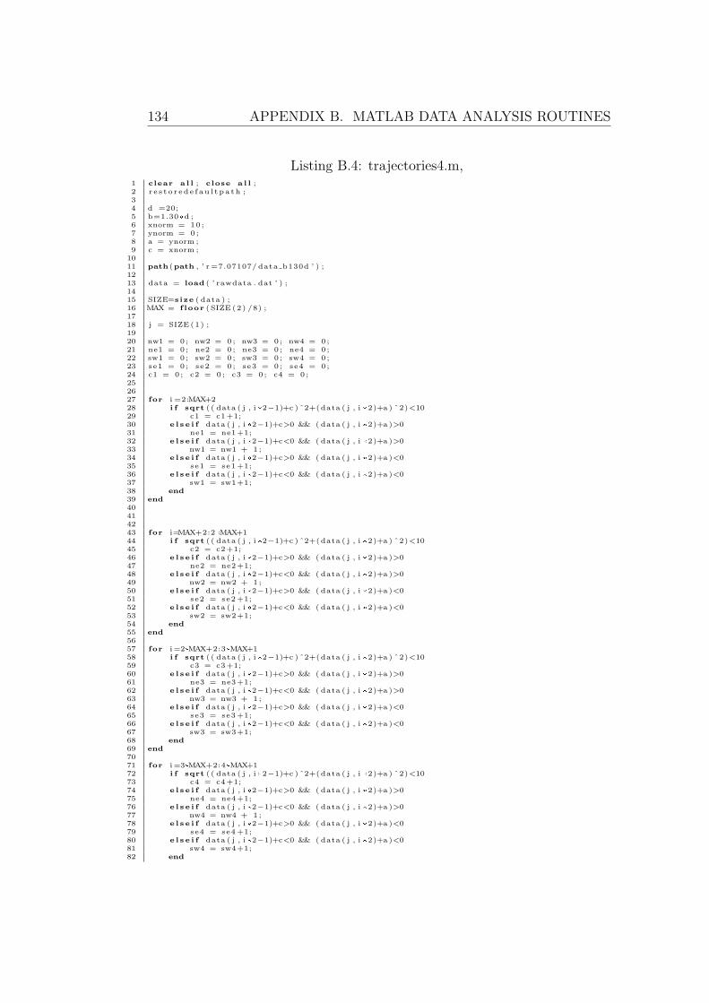
134 APPENDIX B. MATLAB DATA ANALYSIS ROUTINES
Listing B.4: trajectories4.m,1 clear a l l ; close a l l ;2 r e s t o r ed e f au l t p a th ;34 d =20;5 b=1.30*d ;6 xnorm = 10 ;7 ynorm = 0 ;8 a = ynorm ;9 c = xnorm ;
1011 path (path , ’ r =7.07107/ data b130d ’ ) ;1213 data = load ( ’ rawdata . dat ’ ) ;1415 SIZE=s ize ( data ) ;16 MAX = f loor ( SIZE (2) /8) ;1718 j = SIZE (1) ;1920 nw1 = 0 ; nw2 = 0 ; nw3 = 0 ; nw4 = 0 ;21 ne1 = 0 ; ne2 = 0 ; ne3 = 0 ; ne4 = 0 ;22 sw1 = 0 ; sw2 = 0 ; sw3 = 0 ; sw4 = 0 ;23 se1 = 0 ; se2 = 0 ; se3 = 0 ; se4 = 0 ;24 c1 = 0 ; c2 = 0 ; c3 = 0 ; c4 = 0 ;252627 for i =2:MAX+228 i f sqrt ( ( data ( j , i *2−1)+c ) ˆ2+(data ( j , i *2)+a ) ˆ2)<1029 c1 = c1+1;30 e l s e i f data ( j , i *2−1)+c>0 && ( data ( j , i *2)+a )>031 ne1 = ne1+1;32 e l s e i f data ( j , i *2−1)+c<0 && ( data ( j , i *2)+a )>033 nw1 = nw1 + 1 ;34 e l s e i f data ( j , i *2−1)+c>0 && ( data ( j , i *2)+a )<035 se1 = se1 +1;36 e l s e i f data ( j , i *2−1)+c<0 && ( data ( j , i *2)+a )<037 sw1 = sw1+1;38 end39 end40414243 for i=MAX+2:2*MAX+144 i f sqrt ( ( data ( j , i *2−1)+c ) ˆ2+(data ( j , i *2)+a ) ˆ2)<1045 c2 = c2+1;46 e l s e i f data ( j , i *2−1)+c>0 && ( data ( j , i *2)+a )>047 ne2 = ne2+1;48 e l s e i f data ( j , i *2−1)+c<0 && ( data ( j , i *2)+a )>049 nw2 = nw2 + 1 ;50 e l s e i f data ( j , i *2−1)+c>0 && ( data ( j , i *2)+a )<051 se2 = se2 +1;52 e l s e i f data ( j , i *2−1)+c<0 && ( data ( j , i *2)+a )<053 sw2 = sw2+1;54 end55 end5657 for i =2*MAX+2:3*MAX+158 i f sqrt ( ( data ( j , i *2−1)+c ) ˆ2+(data ( j , i *2)+a ) ˆ2)<1059 c3 = c3+1;60 e l s e i f data ( j , i *2−1)+c>0 && ( data ( j , i *2)+a )>061 ne3 = ne3+1;62 e l s e i f data ( j , i *2−1)+c<0 && ( data ( j , i *2)+a )>063 nw3 = nw3 + 1 ;64 e l s e i f data ( j , i *2−1)+c>0 && ( data ( j , i *2)+a )<065 se3 = se3 +1;66 e l s e i f data ( j , i *2−1)+c<0 && ( data ( j , i *2)+a )<067 sw3 = sw3+1;68 end69 end7071 for i =3*MAX+2:4*MAX+172 i f sqrt ( ( data ( j , i *2−1)+c ) ˆ2+(data ( j , i *2)+a ) ˆ2)<1073 c4 = c4+1;74 e l s e i f data ( j , i *2−1)+c>0 && ( data ( j , i *2)+a )>075 ne4 = ne4+1;76 e l s e i f data ( j , i *2−1)+c<0 && ( data ( j , i *2)+a )>077 nw4 = nw4 + 1 ;78 e l s e i f data ( j , i *2−1)+c>0 && ( data ( j , i *2)+a )<079 se4 = se4 +1;80 e l s e i f data ( j , i *2−1)+c<0 && ( data ( j , i *2)+a )<081 sw4 = sw4+1;82 end
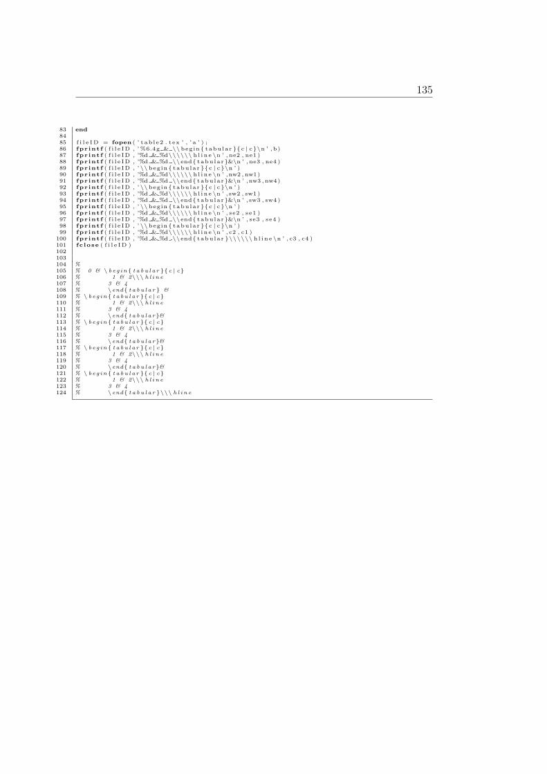
135
83 end8485 f i l e ID = fopen ( ’ t ab l e2 . tex ’ , ’ a ’ ) ;86 fpr int f ( f i l e ID , ’%6.4g & \\begin tabu lar c | c\n ’ ,b)87 fpr int f ( f i l e ID , ’%d & %d\\\\\\ h l i n e \n ’ , ne2 , ne1 )88 fpr int f ( f i l e ID , ’%d & %d \\end tabu lar&\n ’ , ne3 , ne4 )89 fpr int f ( f i l e ID , ’\\begin tabu lar c | c\n ’ )90 fpr int f ( f i l e ID , ’%d & %d\\\\\\ h l i n e \n ’ ,nw2 , nw1)91 fpr int f ( f i l e ID , ’%d & %d \\end tabu lar&\n ’ ,nw3 , nw4)92 fpr int f ( f i l e ID , ’\\begin tabu lar c | c\n ’ )93 fpr int f ( f i l e ID , ’%d & %d\\\\\\ h l i n e \n ’ , sw2 , sw1 )94 fpr int f ( f i l e ID , ’%d & %d \\end tabu lar&\n ’ , sw3 , sw4 )95 fpr int f ( f i l e ID , ’\\begin tabu lar c | c\n ’ )96 fpr int f ( f i l e ID , ’%d & %d\\\\\\ h l i n e \n ’ , se2 , se1 )97 fpr int f ( f i l e ID , ’%d & %d \\end tabu lar&\n ’ , se3 , se4 )98 fpr int f ( f i l e ID , ’\\begin tabu lar c | c\n ’ )99 fpr int f ( f i l e ID , ’%d & %d\\\\\\ h l i n e \n ’ , c2 , c1 )
100 fpr int f ( f i l e ID , ’%d & %d \\end tabu lar \\\\\\ h l i n e \n ’ , c3 , c4 )101 fc lose ( f i l e ID )102103104 %105 % 0 & \ b e g in t a b u l a r c | c106 % 1 & 2\\\ h l i n e107 % 3 & 4108 % \end t a b u l a r &109 % \ b e g in t a b u l a r c | c110 % 1 & 2\\\ h l i n e111 % 3 & 4112 % \end t a b u l a r&113 % \ b e g in t a b u l a r c | c114 % 1 & 2\\\ h l i n e115 % 3 & 4116 % \end t a b u l a r&117 % \ b e g in t a b u l a r c | c118 % 1 & 2\\\ h l i n e119 % 3 & 4120 % \end t a b u l a r&121 % \ b e g in t a b u l a r c | c122 % 1 & 2\\\ h l i n e123 % 3 & 4124 % \end t a b u l a r \\\ h l i n e
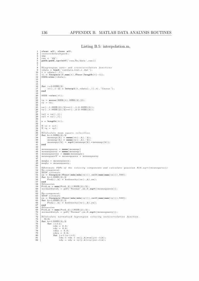
136 APPENDIX B. MATLAB DATA ANALYSIS ROUTINES
Listing B.5: interpolation.m,1 clear a l l ; close a l l ;2 r e s t o r ed e f au l t p a th ;3 t ic4 run = ’ 1Q’ ;5 path (path , sprintf ( ’ run %s/data ’ , run ) )678 %Lagrangian auto− and c r o s s c o r r e l a t i o n f u n c t i o n s9 vdata = load ( ’ r awdata te s t v . dat ’ ) ;
10 t = vdata ( : , 1 ) ;11 t i = linspace (0 ,max( t ) , f loor ( length ( t )−1) ) ;12 SIZE=s ize ( vdata ) ;13141516 for i =3:SIZE (2)17 v i ( : , i −2) = interp1 ( t , vdata ( : , i ) , t i , ’ l i n e a r ’ ) ;18 end1920 SIZE =s ize ( v i ) ;2122 vx = zeros ( SIZE (1) , SIZE (2) /2) ;23 vy = vx ;2425 vx ( : , 1 : SIZE (2) /2)=v i ( : , 1 : 2 : SIZE (2) ) ;26 vy ( : , 1 : SIZE (2) /2)=v i ( : , 2 : 2 : SIZE (2) ) ;2728 vx1 = vx ( : , 1 ) ;29 vy1 = vy ( : , 1 ) ;3031 n = length ( t i ) ;3233 % vx = vx1 ;34 % vy = vy1 ;3536 %Ca l c u l a t e mean square v e l o c i t i e s37 for k=1:SIZE (2) /238 meansqx (k ) = mean( vx ( : , k ) . ˆ 2 ) ;39 meansqy (k ) = mean( vy ( : , k ) . ˆ 2 ) ;40 meansqxy (k ) = sqrt (meansqx (k ) .*meansqy (k ) ) ;41 end4243 meansquarex = mean(meansqx )44 meansquarey = mean(meansqy )45 meansquarexy = mean(meansqxy )46 meansquareV = meansquarex + meansquarey4748 msqLx = meansquarex ;49 msqLy = meansquarey ;5051 %Est imate PDFs o f t h e v e l o c i t y components and c a l c u l a t e gau s s i an N(0 , s q r t ( meansqurex ) )52 %x−component :53 %PDF es t ima t e54 xn = linspace ( f loor (min(min( vx ) ) ) , ce i l (max(max( vx ) ) ) ,500) ;55 for k=1:SIZE (2) /256 FvxL ( : , k ) = ksdens i ty ( vx ( : , k ) , xn ) ;57 end58 %Gaussian59 FvxL m = sum(FvxL , 2 ) /(SIZE (2) /2) ;60 normaldistxL = pdf ( ’Normal ’ , xn , 0 , sqrt ( meansquarex ) ) ;6162 %y−component :63 %PDF es t ima t e64 yn = linspace ( f loor (min(min( vy ) ) ) , ce i l (max(max( vy ) ) ) ,500) ;65 for k=1:SIZE (2) /266 FvyL ( : , k ) = ksdens i ty ( vy ( : , k ) , yn ) ;67 end68 %Gaussian69 FvyL m = sum(FvyL , 2 ) /(SIZE (2) /2) ;70 normaldistyL = pdf ( ’Normal ’ , yn , 0 , sqrt ( meansquarey ) ) ;7172 %Ca l c u l a t e norma l i z ed l a g r an g i an v e l o c i t y a u t o c o r r e l a t i o n f un c t i o n .73 N=0;74 for k=1:SIZE (2) /275 for i =1:n ;76 vdx = 0 . 0 ;77 vdy = 0 . 0 ;78 vdxy = 0 . 0 ;79 vdyx = 0 . 0 ;80 for j =1:(n−i +1)81 vdx = vdx + vx ( j , k ) *vx ( j+i −1,k ) ;82 vdy = vdy + vy ( j , k ) *vy ( j+i −1,k ) ;
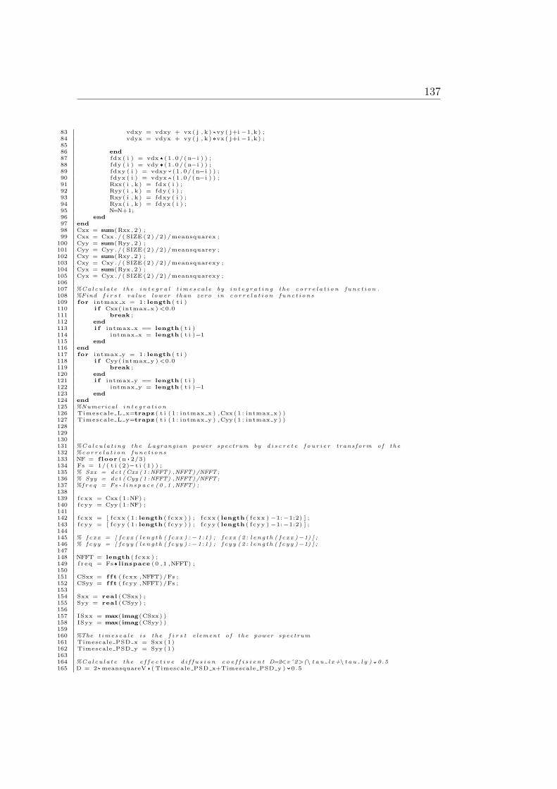
137
83 vdxy = vdxy + vx ( j , k ) *vy ( j+i −1,k ) ;84 vdyx = vdyx + vy ( j , k ) *vx ( j+i −1,k ) ;8586 end87 fdx ( i ) = vdx * ( 1 . 0 / ( n−i ) ) ;88 fdy ( i ) = vdy * ( 1 . 0 / ( n−i ) ) ;89 fdxy ( i ) = vdxy * ( 1 . 0 / ( n−i ) ) ;90 fdyx ( i ) = vdyx * ( 1 . 0 / ( n−i ) ) ;91 Rxx( i , k ) = fdx ( i ) ;92 Ryy( i , k ) = fdy ( i ) ;93 Rxy( i , k ) = fdxy ( i ) ;94 Ryx( i , k ) = fdyx ( i ) ;95 N=N+1;96 end97 end98 Cxx = sum(Rxx , 2 ) ;99 Cxx = Cxx . / ( SIZE (2) /2) /meansquarex ;
100 Cyy = sum(Ryy , 2 ) ;101 Cyy = Cyy . / ( SIZE (2) /2) /meansquarey ;102 Cxy = sum(Rxy , 2 ) ;103 Cxy = Cxy . / ( SIZE (2) /2) /meansquarexy ;104 Cyx = sum(Ryx , 2 ) ;105 Cyx = Cyx . / ( SIZE (2) /2) /meansquarexy ;106107 %Ca l c u l a t e t h e i n t e g r a l t im e s c a l e by i n t e g r a t i n g t h e c o r r e l a t i o n f un c t i o n .108 %Find f i r s t v a l u e l ower than ze ro in c o r r e l a t i o n f u n c t i o n s109 for intmax x = 1 : length ( t i )110 i f Cxx( intmax x )<0.0111 break ;112 end113 i f intmax x == length ( t i )114 intmax x = length ( t i )−1115 end116 end117 for intmax y = 1 : length ( t i )118 i f Cyy( intmax y )<0.0119 break ;120 end121 i f intmax y == length ( t i )122 intmax y = length ( t i )−1123 end124 end125 %Numerical i n t e g r a t i o n126 Timescale L x=trapz ( t i ( 1 : intmax x ) ,Cxx ( 1 : intmax x ) )127 Timescale L y=trapz ( t i ( 1 : intmax y ) ,Cyy ( 1 : intmax y ) )128129130131 %Ca l c u l a t i n g t h e Lagrangian power spectrum by d i s c r e t e f o u r i e r t rans form o f t h e132 %c o r r e l a t i o n f u n c t i o n s133 NF = f loor (n*2/3)134 Fs = 1/( t i (2 )−t i (1 ) ) ;135 % Sxx = dc t (Cxx ( 1 :NFFT) ,NFFT) /NFFT;136 % Syy = dc t (Cyy ( 1 :NFFT) ,NFFT) /NFFT;137 %f r e q = Fs* l i n s p a c e (0 ,1 ,NFFT) ;138139 fcxx = Cxx ( 1 :NF) ;140 fcyy = Cyy ( 1 :NF) ;141142 fcxx = [ fcxx ( 1 : length ( fcxx ) ) ; fcxx ( length ( fcxx ) −1:−1:2) ] ;143 fcyy = [ fcyy ( 1 : length ( fcyy ) ) ; fcyy ( length ( fcyy ) −1:−1:2) ] ;144145 % f c x x = [ f c x x ( l e n g t h ( f c x x ) :−1:1) ; f c x x ( 2 : l e n g t h ( f c x x )−1) ] ;146 % fcy y = [ f c y y ( l e n g t h ( f c y y ) :−1:1) ; f c y y ( 2 : l e n g t h ( f c y y )−1) ] ;147148 NFFT = length ( fcxx ) ;149 f r e q = Fs* linspace (0 ,1 ,NFFT) ;150151 CSxx = f f t ( fcxx ,NFFT)/Fs ;152 CSyy = f f t ( fcyy ,NFFT)/Fs ;153154 Sxx = real (CSxx) ;155 Syy = real (CSyy) ;156157 ISxx = max( imag(CSxx) )158 ISyy = max( imag(CSyy) )159160 %The t ime s c a l e i s t h e f i r s t e l ement o f t h e power spectrum161 Timescale PSD x = Sxx (1)162 Timescale PSD y = Syy (1)163164 %Ca l c u l a t e t h e e f f e c t i v e d i f f u s i o n c o e f f i s i e n t D=2<vˆ2>(\ t a u l x+\ t a u l y ) *0.5165 D = 2*meansquareV *( Timescale PSD x+Timescale PSD y ) *0 .5
138 APPENDIX B. MATLAB DATA ANALYSIS ROUTINES
166167 %Ca l c u l a t e <r ˆ2( t )>=2t<vˆ2>\ i n t 0 ˆ t (1−\ tau / t )R L(\ tau ) d\ tau168 for j =1:n169 rsq ( j ) =2*meansquareV*sum( ( t i ( j )−t i ( 1 : j ) ) ’ . * (Cxx ( 1 : j )+Cyy ( 1 : j ) ) *0 . 5 ) *1/(Fs ) ;170171 end172 sqrsq = sqrt ( r sq ) ;173174 %Plo t c o r r e l a t i o n f u n c t i o n s175 f i g 1 = f igure ;176 set ( gcf , ’ Renderer ’ , ’ p a i n t e r s ’ )177 h=semilogy ( t i , Cxx)178 set (h , ’ LineWidth ’ ,2 )179 hold on180 h=semilogy ( t i , Cyy , ’ r ’ )181 set (h , ’ LineWidth ’ ,2 )182 %h=semi l o gy ( t i , Cxy , ’ g ’ )183 %s e t ( h , ’ LineWidth ’ , 2 )184 %ho ld on185 %h=semi l o gy ( t i , Cyx , ’ c ’ )186 %s e t ( h , ’ LineWidth ’ , 2 )187 legend ( ’Rxx ’ , ’Ryy ’ , ’Rxy ’ , ’Ryx ’ , ’ Locat ion ’ , ’ SouthWest ’ )188 %le g end ( ’ Rxx ’ , ’Ryy ’ , ’ Rxy ’ , ’ Ryx ’ , ’ Locat ion ’ , ’ NorthEast ’ )%Legend f o r 3189 hold o f f190 set (gca , ’ LineWidth ’ ,2 , ’ FontSize ’ ,16)191 grid on192 i f min(Cxx)<0 | | min(Cyy)<0193 axisymin = 1e−3;194 else195 axisymin = min ( [min(Cxx) min(Cyy) ] ) ;196 end197 axis ( [ 0 max( t i ) 1e−2 1 ] )198 t i t l e ( ’ Normalized Lagrangian v e l o c i t y au t o c o r r e l a t i o n func t i on s ’ )199 % savea s ( f i g 1 , s p r i n t f ( ’ run %s / data / p l o t s /AcorrL . f i g ’ , run ) , ’ f i g ’ )200 % savea s ( f i g 1 , s p r i n t f ( ’ run %s / data / p l o t s /AcorrL . eps ’ , run ) , ’ psc2 ’ )201202 %Plo t PDF e s t ima t e s and f i t s203 probdensfuncL = f igure ;204 p1 = semilogy (xn , FvxL m , ’b ’ ) ;205 set (p1 , ’ LineWidth ’ ,2 )206 hold on ;207 norm1 = semilogy (xn , normaldistxL , ’−−b ’ )208 set (norm1 , ’ LineWidth ’ ,2 )209 p2 = semilogy (yn , FvyL m , ’ r ’ ) ;210 set (p2 , ’ LineWidth ’ ,2 )211 norm2 = semilogy (yn , normaldistyL , ’−−r ’ )212 set (norm2 , ’ LineWidth ’ ,2 )213 set (gca , ’ LineWidth ’ ,2 , ’ FontSize ’ ,16)214 p leg = legend ( ’ v x PDF est imate ’ , ’N(0 , sq r t (<v xˆ2>) ) ’ , ’ v y PDF est imate ’ , ’N(0 , sq r t (<v y
ˆ2>) ) ’ )215 set ( pleg , ’ I n t e r p r e t e r ’ , ’ tex ’ )216 axis ([−3 3 1e−5 max( [max(FvxL m) max(FvyL m) ] ) ] )217 t i t l e ( ’ Lagrangian v e l o c i t y PDFs ’ )218 xlabel ( ’ $v (\ lambda D/ t 0 ) $ ’ , ’ I n t e r p r e t e r ’ , ’LaTeX ’ )219 ylabel ( ’ P robab i l i t y ’ )220 grid on221 hold o f f ;222 % savea s ( probdensfuncL , s p r i n t f ( ’ run %s / data / p l o t s /PDFL. f i g ’ , run ) , ’ f i g ’ )223 % savea s ( probdensfuncL , s p r i n t f ( ’ run %s / data / p l o t s /PDFL. eps ’ , run ) , ’ psc2 ’ )224225 %Plo t power s p e c t r a226 powerspectra = f igure ;227 s1 = loglog ( f r e q ( 1 : f loor ( length ( f r e q ) /2) ) , smooth ( Sxx ( 1 : f loor ( length ( Sxx ) /2) ) ,10) , ’b ’ )228 set ( s1 , ’ LineWidth ’ ,2 )229 hold on230 s2 = loglog ( f r e q ( 1 : f loor ( length ( f r e q ) /2) ) , smooth ( Syy ( 1 : f loor ( length ( Syy ) /2) ) ,10) , ’ r ’ )231 set ( s2 , ’ LineWidth ’ ,2 )232 s f i t = loglog ( f req , ( f r e q .ˆ(−2) ) . /9 , ’−−k ’ )233 set ( s f i t , ’ LineWidth ’ ,2 )234 set (gca , ’ LineWidth ’ ,2 , ’ FontSize ’ ,16)235 grid on ;236 xlabel ( ’ Frequency (1/ t 0 ) ’ )237 ylabel ( ’Power ’ )238 legend ( ’G xx ’ , ’G yy ’ , ’ Freqˆ−2 ’ )239 t i t l e ( ’ Lagrangian power s p e c t r a l dens i ty ’ )240 hold o f f241 axis ( [ 7 e−3 1e2 1e−8 1e2 ] )%ax i s f o r 1242 % savea s ( powerspec t ra , s p r i n t f ( ’ run %s / data / p l o t s /psdL . f i g ’ , run ) , ’ f i g ’ )243 % savea s ( powerspec t ra , s p r i n t f ( ’ run %s / data / p l o t s /psdL . eps ’ , run ) , ’ psc2 ’ )244245 %%%%%%%%%%%%%%%%%%%%%%%%%%%%%%%%%%%%%%%%%%%%%%%%%%%%%%%%%%%%%%%%%%%%%%246 %break ;247
139
248 %Eu l e r i an auto− and c r o s s c o r r e l a t i o n f u n c t i o n s249 vdata = load ( ’ rawdata eu le r . dat ’ ) ;250 t = vdata ( : , 1 ) ;251 t i = linspace (0 ,max( t ) , length ( t )−1) ;252 SIZE=s ize ( vdata ) ;253254 for i =3:SIZE (2)255 v i ( : , i −2) = interp1 ( t , vdata ( : , i ) , t i , ’ l i n e a r ’ ) ;256 end257258 SIZE =s ize ( v i ) ;259260 vx = zeros ( SIZE (1) , SIZE (2) /2) ;261 vy = vx ;262263 vx ( : , 1 : SIZE (2) /2)=v i ( : , 1 : 2 : SIZE (2) ) ;264 vy ( : , 1 : SIZE (2) /2)=v i ( : , 2 : 2 : SIZE (2) ) ;265266 vx1 = vx ( : , 1 ) ;267 vy1 = vy ( : , 1 ) ;268269 n = length ( t i ) ;270271 % vx = vx1 ;272 % vy = vy1 ;273274 for k=1:SIZE (2) /2275 meansqx (k ) = mean( vx ( : , k ) . ˆ 2 ) ;276 meansqy (k ) = mean( vy ( : , k ) . ˆ 2 ) ;277 meansqxy (k ) = sqrt (meansqx (k ) .*meansqy (k ) ) ;278 end279280 meansquarex = mean(meansqx )281 meansquarey = mean(meansqy )282 meansquarexy = mean(meansqxy )283284 msqEx = meansquarex ;285 msqEy = meansquarey ;286287 xn = linspace ( f loor (min(min( vx ) ) ) , ce i l (max(max( vx ) ) ) ,100) ;288 for k=1:SIZE (2) /2289 FvxE ( : , k ) = ksdens i ty ( vx ( : , k ) , xn ) ;290 end291 FvxE m = sum(FvxE , 2 ) /(SIZE (2) /2) ;292 normaldistxE = pdf ( ’Normal ’ , xn , 0 , sqrt ( meansquarex ) ) ;293294 yn = linspace ( f loor (min(min( vy ) ) ) , ce i l (max(max( vy ) ) ) ,100) ;295 for k=1:SIZE (2) /2296 FvyE ( : , k ) = ksdens i ty ( vy ( : , k ) , yn ) ;297 end298 FvyE m = sum(FvyE , 2 ) /(SIZE (2) /2) ;299 normaldistyE = pdf ( ’Normal ’ , yn , 0 , sqrt ( meansquarey ) ) ;300301 N=0;302 for k=1:SIZE (2) /2303 for i =1:n ;304 vdx = 0 . 0 ;305 vdy = 0 . 0 ;306 vdxy = 0 . 0 ;307 vdyx = 0 . 0 ;308 for j =1:(n−i +1)309 vdx = vdx + vx ( j , k ) *vx ( j+i −1,k ) ;310 vdy = vdy + vy ( j , k ) *vy ( j+i −1,k ) ;311 vdxy = vdxy + vx ( j , k ) *vy ( j+i −1,k ) ;312 vdyx = vdyx + vy ( j , k ) *vx ( j+i −1,k ) ;313314 end315 fdx ( i ) = vdx * ( 1 . 0 / ( n−i ) ) ;316 fdy ( i ) = vdy * ( 1 . 0 / ( n−i ) ) ;317 fdxy ( i ) = vdxy * ( 1 . 0 / ( n−i ) ) ;318 fdyx ( i ) = vdyx * ( 1 . 0 / ( n−i ) ) ;319 Rxx( i , k ) = fdx ( i ) ;320 Ryy( i , k ) = fdy ( i ) ;321 Rxy( i , k ) = fdxy ( i ) ;322 Ryx( i , k ) = fdyx ( i ) ;323 N=N+1;324 end325 end326 Cxx = sum(Rxx , 2 ) ;327 Cxx = Cxx . / ( SIZE (2) /2) /meansquarex ;328 Cyy = sum(Ryy , 2 ) ;329 Cyy = Cyy . / ( SIZE (2) /2) /meansquarey ;330 Cxy = sum(Rxy , 2 ) ;
140 APPENDIX B. MATLAB DATA ANALYSIS ROUTINES
331 Cxy = Cxy . / ( SIZE (2) /2) /meansquarexy ;332 Cyx = sum(Ryx , 2 ) ;333 Cyx = Cyx . / ( SIZE (2) /2) /meansquarexy ;334335 N;336337 %Ca l c u l a t i n g t h e Eu l e r i an power spectrum by d i s c r e t e f o u r i e r t rans form o f t h e338 %c o r r e l a t i o n f u n c t i o n s339 NF = f loor (n*2/3)340 Fs = 1/( t i (2 )−t i (1 ) ) ;341 % Sxx = dc t (Cxx ( 1 :NFFT) ,NFFT) /NFFT;342 % Syy = dc t (Cyy ( 1 :NFFT) ,NFFT) /NFFT;343 %f r e q = Fs* l i n s p a c e (0 ,1 ,NFFT) ;344345 fcxx = Cxx ( 1 :NF) ;346 fcyy = Cyy ( 1 :NF) ;347348 fcxx = [ fcxx ( 1 : length ( fcxx ) ) ; fcxx ( length ( fcxx ) −1:−1:2) ] ;349 fcyy = [ fcyy ( 1 : length ( fcyy ) ) ; fcyy ( length ( fcyy ) −1:−1:2) ] ;350351 % f c x x = [ f c x x ( l e n g t h ( f c x x ) :−1:1) ; f c x x ( 2 : l e n g t h ( f c x x )−1) ] ;352 % fcy y = [ f c y y ( l e n g t h ( f c y y ) :−1:1) ; f c y y ( 2 : l e n g t h ( f c y y )−1) ] ;353354 NFFT = length ( fcxx ) ;355 f r e q = Fs* linspace (0 ,1 ,NFFT) ;356357 CSxx = f f t ( fcxx ,NFFT)/Fs ;358 CSyy = f f t ( fcyy ,NFFT)/Fs ;359360 Sxx = real (CSxx) ;361 Syy = real (CSyy) ;362363 ISxx = max( imag(CSxx) )364 ISyy = max( imag(CSyy) )365366 %The t ime s c a l e i s t h e f i r s t e l ement o f t h e power spectrum367 Timescale E PSD x = Sxx (1)368 Timescale E PSD y = Syy (1)369370 f i g 1 = f igure ;371372 h=loglog ( t i , Cxx , ’b ’ )373 set (h , ’ LineWidth ’ ,2 )374 hold on375 h=loglog ( t i , Cyy , ’ r ’ )376 set (h , ’ LineWidth ’ ,2 )377 %h=l o g l o g ( t i , Cxy , ’ g ’ )378 set (h , ’ LineWidth ’ ,2 )379 %h=l o g l o g ( t i , Cyx , ’ c ’ )380 set (h , ’ LineWidth ’ ,2 )381 legend ( ’Rxx ’ , ’Ryy ’ , ’Cxy ’ , ’Cyx ’ , ’ Locat ion ’ , ’ SouthWest ’ )382 hold o f f383 set (gca , ’ LineWidth ’ ,2 , ’ FontSize ’ ,16)384 t i t l e ( ’ Normalized Euler ian v e l o c i t y au t o c o r r e l a t i o n func t i on s ’ )385 grid on386 i f min(Cxx)<0 | | min(Cyy)<0387 axisyminE = 1e−3;388 e l s e i f min(Cxx)<0.1 | | min(Cyy)<0.1389 axisyminE = min ( [min(Cxx) min(Cyy) ] ) ;390 else391 axisyminE = 0 . 1 ;392 end393 axis ( [ 1 e−3 max( t i ) 1e−2 max( [max(Cxx ( 1 : n−0.1*n) ) max(Cyy ( 1 : n−0.1*n) ) ] ) ] )394 set (gca , ’ YMinorTick ’ , ’ on ’ )395 % savea s ( f i g 1 , s p r i n t f ( ’ run %s / data / p l o t s /AcorrE . f i g ’ , run ) , ’ f i g ’ )396 % savea s ( f i g 1 , s p r i n t f ( ’ run %s / data / p l o t s /AcorrE . eps ’ , run ) , ’ psc2 ’ )397398399 probdensfuncE = f igure ;400 p1 = semilogy (xn , FvxE m , ’b ’ ) ;401 set (p1 , ’ LineWidth ’ ,2 )402 hold on403 norm1 = semilogy (xn , normaldistxE , ’−−b ’ )404 set (norm1 , ’ LineWidth ’ ,2 )405 p2 = semilogy (yn , FvyE m , ’ r ’ ) ;406 set (p2 , ’ LineWidth ’ ,2 )407 norm2 = semilogy (yn , normaldistyE , ’−−r ’ )408 set (norm2 , ’ LineWidth ’ ,2 )409 set (gca , ’ LineWidth ’ ,2 , ’ FontSize ’ ,16)410 p leg = legend ( ’ v x PDF est imate ’ , ’N(0 , sq r t (<v xˆ2>) ) ’ , ’ v y PDF est imate ’ , ’N(0 , sq r t (<v y
ˆ2>) ) ’ )411 set ( pleg , ’ I n t e r p r e t e r ’ , ’ tex ’ )412 axis ([−3 3 1e−5 max( [max(FvxE m) max(FvyE m) ] ) ] )
141
413 %ax i s ([−7 7 1e−4 1 . 5 ] )%a x i s f o r 05Q414 t i t l e ( ’ Eu le r ian v e l o c i t y PDFs ’ )415 xlabel ( ’ $v (\ lambda D/ t 0 ) $ ’ , ’ I n t e r p r e t e r ’ , ’LaTeX ’ )416 ylabel ( ’ P robab i l i t y ’ )417 grid on418 hold o f f419 % savea s ( probdensfuncE , s p r i n t f ( ’ run %s / data / p l o t s /PDFE. f i g ’ , run ) , ’ f i g ’ )420 % savea s ( probdensfuncE , s p r i n t f ( ’ run %s / data / p l o t s /PDFE. eps ’ , run ) , ’ psc2 ’ )421422 %Plo t power s p e c t r a423 powerspectra = f igure ;424 s1 = loglog ( f r e q ( 1 : f loor ( length ( f r e q ) /2) ) , smooth ( Sxx ( 1 : f loor ( length ( Sxx ) /2) ) ,10) , ’b ’ )425 set ( s1 , ’ LineWidth ’ ,2 )426 hold on427 s2 = loglog ( f r e q ( 1 : f loor ( length ( f r e q ) /2) ) , smooth ( Syy ( 1 : f loor ( length ( Syy ) /2) ) ,10) , ’ r ’ )428 set ( s2 , ’ LineWidth ’ ,2 )429 s f i t = loglog ( f req , ( f r e q .ˆ(−1) ) . /9 , ’−−k ’ )430 set ( s f i t , ’ LineWidth ’ ,2 )431 set (gca , ’ LineWidth ’ ,2 , ’ FontSize ’ ,16)432 grid on ;433 xlabel ( ’ Frequency (1/ t 0 ) ’ )434 ylabel ( ’Power ’ )435 legend ( ’G xx ’ , ’G yy ’ , ’ Freqˆ−1 ’ )436 t i t l e ( ’ Eu le r ian power s p e c t r a l dens i ty ’ )437 hold o f f438 axis ( [ 5 e−3 1e2 1e−5 1e2 ] )%ax i s f o r 1439 % savea s ( powerspec t ra , s p r i n t f ( ’ run %s / data / p l o t s /psdE . f i g ’ , run ) , ’ f i g ’ )440 % savea s ( powerspec t ra , s p r i n t f ( ’ run %s / data / p l o t s /psdE . eps ’ , run ) , ’ psc2 ’ )441442443444 %%Write mean square v e l o c i t i e s L & E to f i l e f o r comparison . Used on the445 %%data w i th random seed446 f i l e ID = fopen ( ’ vmeansquaredata . dat ’ , ’ a ’ ) ;447 fpr int f ( f i l e ID , ’%d %f %f %f %f \n ’ , ( ( run )+1) ,msqLx , msqLy ,msqEx ,msqEy) ;448 fc lose ( f i l e ID ) ;449450 %%Write t h e E&L PSD t im e s c a l e s to f i l e . For use w i th t h e random seed data .451 % f i l e I D=fopen ( ’ ELt imesca l e s . dat ’ , ’ a ’ ) ;452 % f p r i n t f ( f i l e ID , ’%d %f %f %f %f \n ’ , ( ( run )+1) , Timescale PSD x , Timescale PSD y ,
Timescale E PSD x , Timescale E PSD y ) ;453 % f c l o s e ( f i l e I D ) ;454455 %%Write s q r t (<r ˆ2( t )>) to f i l e . Used f o r t h e runs w i th d i f f e r e n t Q456 % f i l e I D = fopen ( s p r i n t f ( ’ rms r ( t )%s . dat ’ , run ) , ’w ’ ) ;457 % A = [ t i ; s q r s q ] ;458 % f p r i n t f ( f i l e ID , ’% f %f \n ’ ,A) ;459 % f c l o s e ( f i l e I D ) ;460 %461 %%Write t h e mean square v e l o c i t i e s (L) to f i l e . Used f o r t h e runs w i th462 %%d i f f e r e n t Q463 % f i l e I D = fopen ( ’ vmeansquare varQ . dat ’ , ’ a ’ ) ;464 % f p r i n t f ( f i l e ID , ’% f \n ’ , meansquareV )465 % f c l o s e ( f i l e I D )466 %467 %%Write t h e numer i c a l l y i n t e g r a t e d t im e s c a l e s to f i l e . For t h e runs w i th468 %%d i f f e r e n t Q469 % f i l e I D = fopen ( ’ t i m e s c a l e s i n t e g r a t e d . dat ’ , ’ a ’ ) ;470 % f p r i n t f ( f i l e ID , ’% s %f %f \n ’ , run , Timesca le L x , T imesca l e L y ) ;471 % f c l o s e ( f i l e I D ) ;472 %473 %%Write t h e PSD t im e s c a l e s to f i l e . For t h e runs w i th474 %%d i f f e r e n t Q475 % f i l e I D = fopen ( ’ t im e s c a l e s p s d (0) . dat ’ , ’ a ’ ) ;476 % f p r i n t f ( f i l e ID , ’% s %f %f \n ’ , run , Timescale PSD x , Timescale PSD y ) ;477 % f c l o s e ( f i l e I D ) ;478 %479 %%Write t h e d i f f u s i o n c o e f f i s i e n t s to f i l e . For t h e runs w i th d i f f e r e n t Q480 % f i l e I D = fopen ( ’ d i f f u s i o n c o e f f i s i e n t s . dat ’ , ’ a ’ ) ;481 % f p r i n t f ( f i l e ID , ’% s %f \n ’ , run ,D) ;482 % f c l o s e ( f i l e I D )483484485486 r e s t o r ed e f au l t p a th ;487488 toc489 r e s t o r ed e f au l t p a th ;
142 APPENDIX B. MATLAB DATA ANALYSIS ROUTINES
Listing B.6: meansquareplot.m,1 clear a l l ; close a l l ;23 vmean = load ( ’ vmeansquaredata . dat ’ ) ;4 vmeans = [ ] ;56 for i =1: s ize (vmean , 1 )7 vmeans = [ vmeans ; vmean( i , 2 ) vmean( i , 4 ) ; vmean( i , 3 ) vmean( i , 5 ) ] ;8 end9 f igure ;
10 hold on ;11 for i =1: s ize ( vmeans , 1 ) /212 h = plot ( vmeans ( i *2−1: i *2 ,1) , vmeans ( i *2−1: i *2 ,2) , ’−xk ’ ) ;13 set (h , ’ LineWidth ’ ,2 )14 end15 h=plot ( vmeans ( : , 1 ) , vmeans ( : , 2 ) , ’ x ’ )16 h=plot (vmean ( : , 2 ) ,vmean ( : , 4 ) , ’ xb ’ ) ;17 set (h , ’ LineWidth ’ ,2 )18 h=plot (vmean ( : , 3 ) ,vmean ( : , 5 ) , ’ xr ’ ) ;19 set (h , ’ LineWidth ’ ,2 )20 set (gca , ’ LineWidth ’ ,2 , ’ FontSize ’ ,16)21 xlabel ( ’<v Lˆ2> ’ )22 ylabel ( ’<v Eˆ2> ’ )23 axis ( [ 0 0 .22 0 0 . 8 ] ) ;24 grid on25 h=plot ( 0 . 1009 , 0 . 2107 , ’ sb ’ )26 set (h , ’ LineWidth ’ ,3 , ’ MarkerSize ’ ,6 )27 h=plot ( 0 . 0941 , 0 . 2088 , ’ s r ’ )28 set (h , ’ LineWidth ’ ,3 , ’ MarkerSize ’ ,6 )29 h=plot ( [ 0 : 0 . 0 1 : 0 . 2 2 ] , [ 0 : 0 . 0 1 : 0 . 2 2 ] , ’−.k ’ )30 set (h , ’ LineWidth ’ ,2 )31 hold o f f3233 % uL = ( vmean ( : , 2 )+vmean ( : , 3 ) ) *0 . 5 ;34 % uE = ( vmean ( : , 4 )+vmean ( : , 5 ) ) *0 . 5 ;35 %36 % f i g u r e37 % h = p l o t (uL , uE , ’ x ’ )
143
Listing B.7: timescaleplot.m,1 clear a l l ; close a l l ;2 t = load ( ’ ELtimescales . dat ’ ) ;3 tml = mean ( [ t ( : , 2 ) t ( : , 3 ) ] , 2 ) ;4 tme = mean ( [ t ( : , 4 ) t ( : , 5 ) ] , 2 ) ;5 hold on6 h=plot ( tml , tme , ’ o ’ ) ;7 set (h , ’ LineWidth ’ ,6 , ’ MarkerSize ’ ,4 )8 h =plot (mean( tml ) ,mean( tme ) , ’+r ’ ) ;9 set (h , ’ LineWidth ’ ,3 , ’ MarkerSize ’ ,10)
10 set (gca , ’ LineWidth ’ ,2 , ’ FontSize ’ ,16)11 h=plot (0 .5* (13 .998705+8.900086) ,0 .5* (14 .201664+2.066290 e+01) , ’ s ’ )12 set ( get ( get (h , ’ Annotation ’ ) , ’ LegendInformation ’ ) , ’ I conDi sp laySty l e ’ , ’ o f f ’ )13 set (h , ’ LineWidth ’ ,6 , ’ MarkerSize ’ ,4 )14 grid on15 f i t o = f i t ( tml , tme , ’ poly1 ’ ) ;16 h=plot ( f i t o , ’−−k ’ )17 set (h , ’ LineWidth ’ ,2 )18 axis ( [ 0 16 0 18 ] )19 legend ( ’ (\ tau L ,\ tau E ) ’ , ’ (<\tau L>,<\tau E>) ’ , sprintf ( ’ y=%6.3gx +%6.3g ’ , f i t o . p1 , f i t o . p2
) , ’ Locat ion ’ , ’ NorthWest ’ )20 xlabel ( ’\ tau L ’ )21 ylabel ( ’\ tau E ’ )22 hold o f f
144 APPENDIX B. MATLAB DATA ANALYSIS ROUTINES
Listing B.8: timescales.m,1 clear a l l ; close a l l ;23 T in = load ( ’ t ime s c a l e s i n t e g r a t e d . dat ’ ) ;4 T psd = load ( ’ t ime s ca l e s p sd (0) . dat ’ ) ;5 Dc = load ( ’ d i f f u s i o n c o e f f i s i e n t s . dat ’ ) ;6 D = Dc ( : , 2 ) ;7 vmsq = load ( ’ vmeansquare varQ . dat ’ ) ;8 q = [ 0 . 1 0 .05 0 .025 0.0125 0 . 0 0 6 2 5 ] ;9
101112 f i g 1 = f igure ;13 h = loglog (q , T in ( : , 2 ) , ’−xb ’ )14 set (h , ’ LineWidth ’ ,2 )15 hold on16 h = loglog (q , T in ( : , 3 ) , ’−xr ’ )17 set (h , ’ LineWidth ’ ,2 )18 h = loglog (q , 0 . 5 . * ( T in ( : , 2 )+T in ( : , 3 ) ) , ’−xk ’ )19 set (h , ’ LineWidth ’ ,2 )20 h = loglog (q , 1 . / q , ’−−k ’ )21 set (h , ’ LineWidth ’ ,2 )22 h = loglog (q , 2 . / sqrt ( q ) , ’−.k ’ )23 set (h , ’ LineWidth ’ ,2 )24 set (gca , ’ LineWidth ’ ,2 , ’ FontSize ’ ,16)25 xlabel ( ’ Vortex s t r ength (\gamma) ’ )26 ylabel ( ’ Timescale (\gamma) ’ )27 legend ( ’\ tau Lx ’ , ’\ tau Ly ’ , ’\ tau L ’ , ’\gammaˆ−1 ’ , ’ 2*\gammaˆ−1/2 ’ , ’ Locat ion ’ , ’
SouthWest ’ )28 t i t l e ( ’ Numerical ly i n t eg ra t ed t ime s ca l e s ’ )29 axis ( [ 0 . 0 0625 0 .1 min( T in ( : , 3 ) ) max( T in ( : , 2 ) ) ] )30 grid on31 hold o f f32 saveas ( f i g1 , ’ t ime s c a l e s . f i g ’ , ’ f i g ’ )33 saveas ( f i g1 , ’ t ime s c a l e s . eps ’ , ’ psc2 ’ )3435 f i g 2 = f igure ;36 h = loglog (q , T psd ( : , 2 ) , ’−xb ’ )37 set (h , ’ LineWidth ’ ,2 )38 hold on39 h = loglog (q , T psd ( : , 3 ) , ’−xr ’ )40 set (h , ’ LineWidth ’ ,2 )41 h = loglog (q , 0 . 5 . * ( T psd ( : , 2 )+T psd ( : , 3 ) ) , ’−xk ’ )42 set (h , ’ LineWidth ’ ,2 )43 h = loglog (q , 1 . / q , ’−−k ’ )44 set (h , ’ LineWidth ’ ,2 )45 h = loglog (q , 2 . / sqrt ( q ) , ’−.k ’ )46 set (h , ’ LineWidth ’ ,3 )47 set (gca , ’ LineWidth ’ ,2 , ’ FontSize ’ ,16)48 xlabel ( ’ Vortex s t r ength (\gamma) ’ )49 ylabel ( ’ Timescale (\gamma) ’ )50 legend ( ’\ tau Lx ’ , ’\ tau Ly ’ , ’\ tau L ’ , ’\gammaˆ−1 ’ , ’ 2\gammaˆ−1/2 ’ , ’ Locat ion ’ , ’
SouthWest ’ )51 t i t l e ( ’ Timescales from PSD( f =0) ’ )52 axis ( [ 0 . 0 0625 0 .1 min( T psd ( : , 3 ) ) max( T psd ( : , 2 ) ) ] )53 grid on54 hold o f f55 saveas ( f i g2 , ’ t ime s ca l e s p sd . f i g ’ , ’ f i g ’ )56 saveas ( f i g2 , ’ t ime s ca l e s p sd . eps ’ , ’ psc2 ’ )5758 f i g 3 = f igure ;59 h = loglog (q ,D, ’−xb ’ )60 set (h , ’ LineWidth ’ ,2 )61 hold on62 h = loglog (q , 30*5 . 5* q . ˆ ( 3/2 ) , ’−−k ’ )63 set (h , ’ LineWidth ’ ,2 )64 set (gca , ’ LineWidth ’ ,2 , ’ FontSize ’ ,16)65 axis ( [ 0 . 0 0625 0 .1 min(D) max(D) ] )66 xlabel ( ’ Vortex s t r ength (\gamma) ’ )67 ylabel ( ’ D i f f u s i on c o e f f i s i e n t ’ )68 legend ( ’D(\gamma) ’ , ’ 165*\gammaˆ3/2 ’ , ’ Locat ion ’ , ’ SouthEast ’ )69 grid on70 hold o f f71 saveas ( f i g3 , ’ d i f f u s i o n c o e f f i s i e n t s Q . f i g ’ , ’ f i g ’ )72 saveas ( f i g3 , ’ d i f f u s i o n c o e f f i s i e n t s Q . eps ’ , ’ psc2 ’ )7374 f i g 4 = f igure ;7576 h = loglog (q , 10*0 . 5* q , ’−−k ’ )77 set (h , ’ LineWidth ’ ,2 )78 hold on79 h = loglog (q , sqrt (vmsq) , ’−xb ’ )80 set (h , ’ LineWidth ’ ,2 )
145
81 set (gca , ’ LineWidth ’ ,2 , ’ FontSize ’ ,16)82 xlabel ( ’ Vortex s t r ength (\gamma) ’ )83 ylabel ( ’(<v Lˆ2>)ˆ1/2 ’ )84 legend ( ’ 5*\gamma ’ , ’ (<v Lˆ2>)ˆ1/2 ’ , ’ Locat ion ’ , ’ SouthEast ’ )85 axis ( [min( q ) max( q ) min( sqrt (vmsq) ) max( sqrt (vmsq) ) ] )86 grid on87 hold o f f88 saveas ( f i g4 , ’ rmsv . f i g ’ , ’ f i g ’ )89 saveas ( f i g4 , ’ rmsv . eps ’ , ’ psc2 ’ )9091 f i g 5 = f igure ;92 h = loglog ( sqrt (vmsq) ,D, ’−xb ’ )93 set (h , ’ LineWidth ’ ,2 )94 hold on95 h = loglog ( sqrt (vmsq) ,7* ( vmsq . ˆ ( 1/2 ) ) , ’−−k ’ )96 set (h , ’ LineWidth ’ ,2 )97 %h=l o g l o g ( )98 set (gca , ’ LineWidth ’ ,2 , ’ FontSize ’ ,16)99 xlabel ( ’(<v Lˆ2>)ˆ1/2 ’ )
100 ylabel ( ’ D i f f u s i on c o e f f i s i e n t ’ )101 legend ( ’D ’ , ’ 7*(<v Lˆ2>)ˆ1/2 ’ , ’ Locat ion ’ , ’ SouthEast ’ )102 %ax i s ( [ 1 e−2 1e0 1e−1 1e1 ] )103 axis ( [min( sqrt (vmsq) ) max( sqrt (vmsq) ) 1e−1 1e1 ] )104 grid on105 hold o f f106 saveas ( f i g5 , ’ d i f f u s i o n c o e f f i s i e n t s v r m s . f i g ’ , ’ f i g ’ )107 saveas ( f i g5 , ’ d i f f u s i o n c o e f f i s i e n t s v r m s . eps ’ , ’ psc2 ’ )
146 APPENDIX B. MATLAB DATA ANALYSIS ROUTINES
Listing B.9: rmsr.m,1 clear a l l ; close a l l ;23 rms1q = load ( ’ rms r ( t ) 1Q. dat ’ ) ;4 rms05q = load ( ’ rms r ( t ) 05Q. dat ’ ) ;5 rms025q = load ( ’ rms r ( t ) 025Q. dat ’ ) ;6 rms0125q = load ( ’ rms r ( t ) 0125Q. dat ’ ) ;7 rms00625q = load ( ’ rms r ( t ) 00625Q. dat ’ ) ;89 f i g = f igure
10 h=loglog ( rms1q ( : , 1 ) , rms1q ( : , 2 ) )11 set (h , ’ LineWidth ’ ,2 )12 hold on13 h=loglog ( rms05q ( : , 1 ) , rms05q ( : , 2 ) , ’ r ’ )14 set (h , ’ LineWidth ’ ,2 )15 h=loglog ( rms025q ( : , 1 ) , rms025q ( : , 2 ) , ’ g ’ )16 set (h , ’ LineWidth ’ ,2 )17 h=loglog ( rms0125q ( : , 1 ) , rms0125q ( : , 2 ) , ’ c ’ )18 set (h , ’ LineWidth ’ ,2 )19 h=loglog ( rms00625q ( : , 1 ) , rms00625q ( : , 2 ) , ’m’ )20 set (h , ’ LineWidth ’ ,2 )21 h = loglog ( rms1q ( : , 1 ) , 0 . 5* rms1q ( : , 1 ) , ’−−k ’ )22 set (h , ’ LineWidth ’ ,2 )23 h = loglog ( rms1q ( : , 1 ) , 1 . 5* sqrt ( rms1q ( : , 1 ) ) , ’−−k ’ )24 set (h , ’ LineWidth ’ ,2 )25 set (gca , ’ LineWidth ’ ,2 , ’ FontSize ’ ,16)26 grid on27 xlabel ( ’ t ( t 0 ) ’ )28 ylabel ( ’(<r ˆ2( t )>)ˆ1/2 ’ )29 axis ( [ 2 e−2 1e2 1e−2 3e1 ] )30 legend ( ’\gamma=0.1 ’ , ’\gamma=0.05 ’ , ’\gamma=0.025 ’ , ’\gamma=0.0125 ’ , ’\gamma=0.00625 ’ , ’ 0 .5* t
’ , ’ 1 .5* t ˆ1/2 ’ , ’ Locat ion ’ , ’ NorthWest ’ )31 t i t l e ( ’ Root mean square disp lacement f o r varying va lues o f Q’ )32 hold o f f33 saveas ( f i g , ’ rms r . eps ’ , ’ psc2 ’ ) ;34 saveas ( f i g , ’ rms r . f i g ’ , ’ f i g ’ ) ;
147
Listing B.10: trajectories.m,1 clear a l l ; close a l l ;23 load ( ’ rawdata . dat ’ )4 %load ( ’ r awd a t a t e s t . dat ’ )5 f igure67 SIZE=s ize ( rawdata ) ;8 %s e t ( gc f , ’ De fau l tAxesCo lorOrder ’ , [ 0 0 1 ; 1 0 0 ] )9
10 h=plot ( rawdata ( : , 3 ) , rawdata ( : , 4 ) , ’b ’ ) ;11 set (h , ’ LineWidth ’ ,2 )12 hold on13 h=plot ( rawdata ( : , 5 ) , rawdata ( : , 6 ) , ’ r ’ ) ;14 set (h , ’ LineWidth ’ ,2 )15 h=plot ( rawdata (1 , 3 ) , rawdata (1 ,4 ) , ’<b ’ ) ;16 set (h , ’ LineWidth ’ ,4 )17 h=plot ( rawdata (1 , 5 ) , rawdata (1 ,6 ) , ’>r ’ ) ;18 set (h , ’ LineWidth ’ ,4 )19 h=plot ( rawdata ( : , 7 ) , rawdata ( : , 8 ) , ’b ’ ) ;20 set (h , ’ LineWidth ’ ,2 )21 h=plot ( rawdata ( : , 9 ) , rawdata ( : , 1 0 ) , ’ r ’ ) ;22 set (h , ’ LineWidth ’ ,2 )23 h=plot ( rawdata (1 , 7 ) , rawdata (1 ,8 ) , ’>b ’ ) ;24 set (h , ’ LineWidth ’ ,4 )25 h=plot ( rawdata (1 , 9 ) , rawdata (1 ,10) , ’<r ’ ) ;26 set (h , ’ LineWidth ’ ,4 )272829 % SIZET=s i z e ( r awd a t a t e s t ) ;30 % fo r i =2:SIZET (2) /231 % h=p l o t ( r awd a t a t e s t ( : , i *2−1) , r awd a t a t e s t ( : , i *2) , ’ r ’ ) ;32 % s e t ( h , ’ LineWidth ’ , 2 )33 % ho ld a l l34 % end35 % h2=p l o t ( rawdata ( l e n g t h ( rawdata ) ,3) , rawdata ( l e n g t h ( rawdata ) ,4) , ’ x ’ )36 % h3=p l o t ( rawdata ( l e n g t h ( rawdata ) ,5) , rawdata ( l e n g t h ( rawdata ) ,6) , ’ x ’ )37 % h4=p l o t ( rawdata ( l e n g t h ( rawdata ) ,7) , rawdata ( l e n g t h ( rawdata ) ,8) , ’ x ’ )38 % s e t ( h2 , ’ LineWidth ’ , 4 )39 % s e t ( h3 , ’ LineWidth ’ , 4 )40 % s e t ( h4 , ’ LineWidth ’ , 4 )41 % h5=p l o t ( rawdata (1 ,3 ) , rawdata (1 ,4 ) , ’ ˆ ’ ) ;42 % h6=p l o t ( rawdata (1 ,5 ) , rawdata (1 ,6 ) , ’ v ’ ) ;43 % %h7=p l o t ( rawdata (1 ,7 ) , rawdata (1 ,8 ) , ’ o ’ ) ;44 % s e t ( h5 , ’ LineWidth ’ , 4 )45 % s e t ( h6 , ’ LineWidth ’ , 4 )46 % %s e t ( h7 , ’ LineWidth ’ , 4 )47 set (gca , ’ FontSize ’ ,16 , ’ LineWidth ’ ,2 )48 xlabel ( ’ $x (\ lambda D ) $ ’ , ’ I n t e r p r e t e r ’ , ’LaTeX ’ )49 ylabel ( ’ $y (\ lambda D ) $ ’ , ’ I n t e r p r e t e r ’ , ’LaTeX ’ )50 %le g end ( ’Q=1.0 ’ , ’Q=−0.9 ’)51 grid on52 axis equal53 %ax i s ([−0.5 1 .5 −0.1 2 . 1 ] )