Tutorial on Nonparametric Inference With R - Center for Astrostatistics
202
Tutorial on Nonparametric Inference With R Chad Schafer and Larry Wasserman [email protected] [email protected] Carnegie Mellon University Tutorial on Nonparametric Inference – p.1/202
Transcript of Tutorial on Nonparametric Inference With R - Center for Astrostatistics
Tutorial on NonparametricInference
With R
Chad Schafer and Larry Wasserman
[email protected] [email protected]
Carnegie Mellon University
Tutorial on Nonparametric Inference – p.1/202
Outline
General Concepts of Smoothing, Bias-Variance Tradeoff
Linear Smoothers
Cross Validation
Local Polynomial Regression
Confidence Bands
Basis Methods: Splines and Wavelets
Multiple Regression
Density Estimation
Measurement Error
Inverse Probems
Classification
Nonparametric Bayes Tutorial on Nonparametric Inference – p.2/202
Basic Concepts in Smoothing
Problem I: Regression. Observe (X1, Y1), . . . , (Xn, Yn).Estimate f(x) = E(Y |X = x). Equivalently:
Yi = f(Xi) + εi
where E(εi) = 0. Simple estimator:
f(x) = meanYi : |Xi − x| ≤ h.
Problem II: Density Estimation. Observe X1, . . . , Xn ∼ f .Estimate f . Simple estimator: f(x) = histogram.
Tutorial on Nonparametric Inference – p.3/202
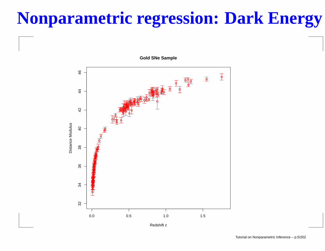
Nonparametric regression: Dark Energy
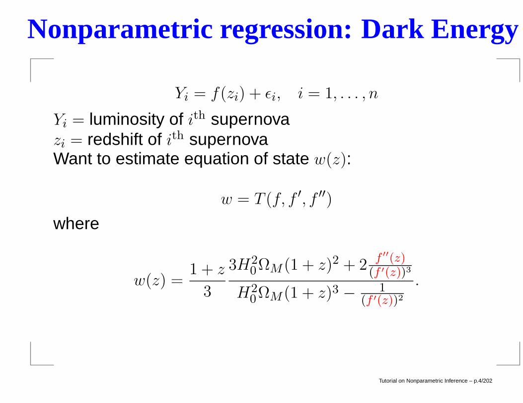
Yi = f(zi) + εi, i = 1, . . . , n
Yi = luminosity of ith supernovazi = redshift of ith supernovaWant to estimate equation of state w(z):
w = T (f, f ′, f ′′)
where
w(z) =1 + z
3
3H20ΩM (1 + z)2 + 2 f ′′(z)
(f ′(z))3
H20ΩM (1 + z)3 − 1
(f ′(z))2.
Tutorial on Nonparametric Inference – p.4/202
Nonparametric regression: Dark Energy
0.0 0.5 1.0 1.5
3234
3638
4042
4446
Gold SNe Sample
Redshift z
Dis
tanc
e M
odul
us
Tutorial on Nonparametric Inference – p.5/202
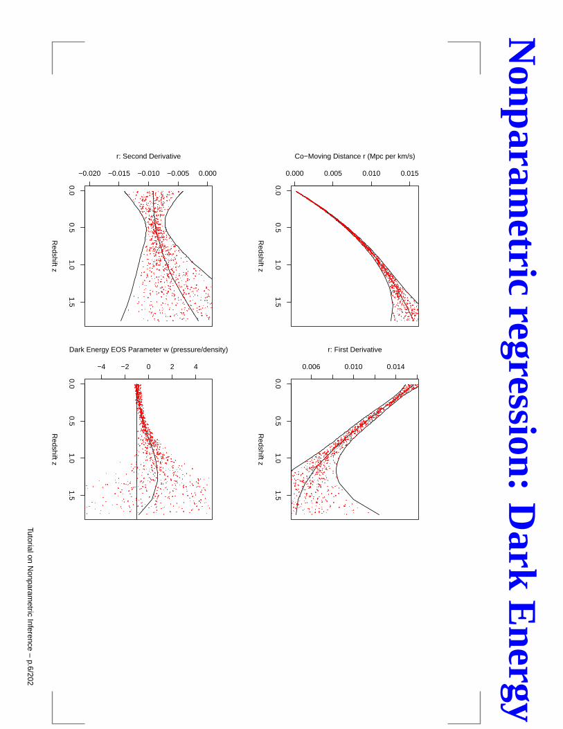
Nonparam
etricregression:
Dark
Energy
0.00.5
1.01.5
0.000 0.005 0.010 0.015
Redshift z
Co−Moving Distance r (Mpc per km/s)
0.00.5
1.01.5
0.006 0.010 0.014
Redshift z
r: First Derivative
0.00.5
1.01.5
−0.020 −0.015 −0.010 −0.005 0.000
Redshift z
r: Second Derivative
0.00.5
1.01.5
−4 −2 0 2 4
Redshift z
Dark Energy EOS Parameter w (pressure/density)
TutorialonN
onparametric
Inference–
p.6/202
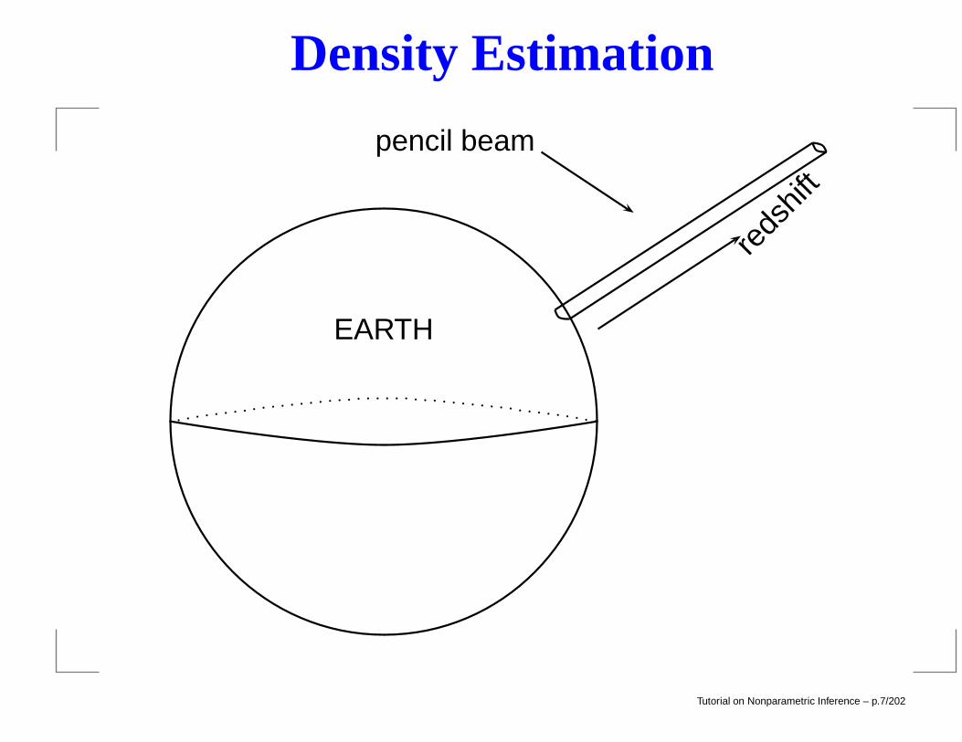
Density Estimation
reds
hift
EARTH
pencil beam
Tutorial on Nonparametric Inference – p.7/202
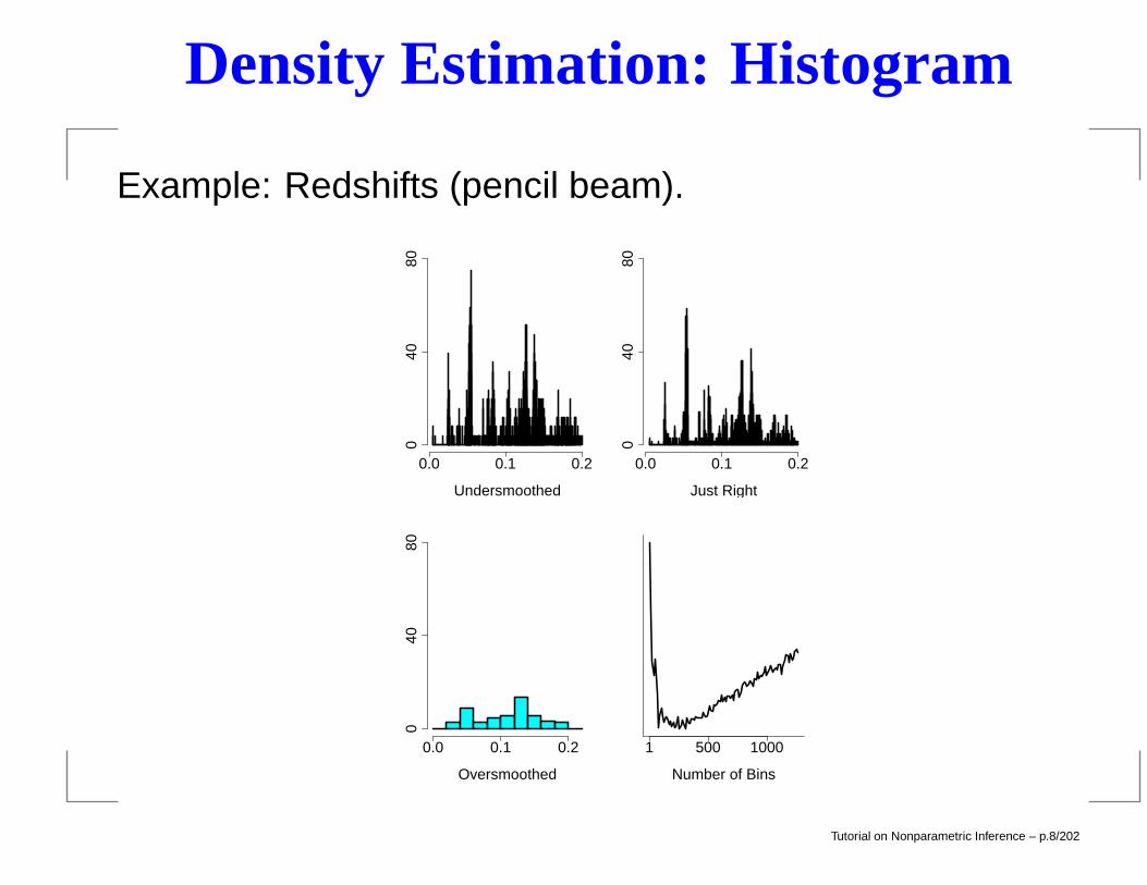
Density Estimation: Histogram
Example: Redshifts (pencil beam).
0.0 0.1 0.2
040
80
Undersmoothed
0.0 0.1 0.2
040
80
Just Right
0.0 0.1 0.2
040
80
Oversmoothed
1 500 1000
Number of Bins
Tutorial on Nonparametric Inference – p.8/202
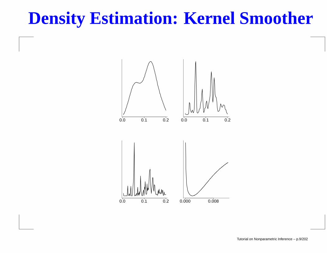
Density Estimation: Kernel Smoother
0.0 0.1 0.2 0.0 0.1 0.2
0.0 0.1 0.2 0.000 0.008
Tutorial on Nonparametric Inference – p.9/202
The Bias–Variance Tradeoff
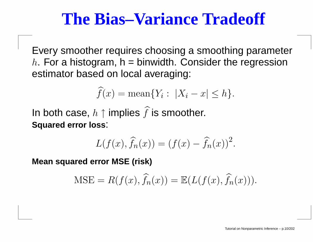
Every smoother requires choosing a smoothing parameterh. For a histogram, h = binwidth. Consider the regressionestimator based on local averaging:
f(x) = meanYi : |Xi − x| ≤ h.
In both case, h ↑ implies f is smoother.Squared error loss:
L(f(x), fn(x)) = (f(x)− fn(x))2.Mean squared error MSE (risk)
MSE = R(f(x), fn(x)) = E(L(f(x), fn(x))).
Tutorial on Nonparametric Inference – p.10/202
The Bias–Variance Tradeoff
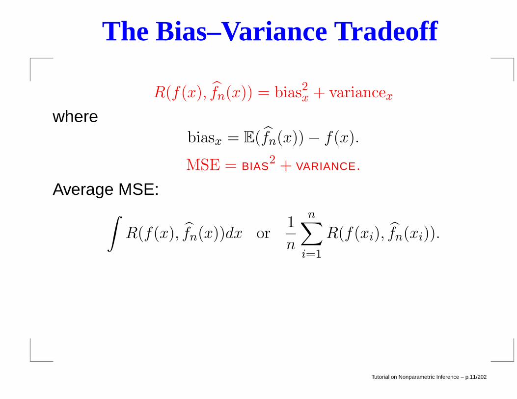
R(f(x), fn(x)) = bias2x + variancex
wherebiasx = E(fn(x))− f(x).
MSE = BIAS2 + VARIANCE.
Average MSE:∫R(f(x), fn(x))dx or
1
n
n∑
i=1
R(f(xi), fn(xi)).
Tutorial on Nonparametric Inference – p.11/202
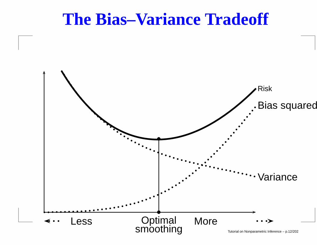
The Bias–Variance Tradeoff
Risk
Bias squared
Variance
Optimalsmoothing
MoreLessTutorial on Nonparametric Inference – p.12/202
The Bias–Variance Tradeoff
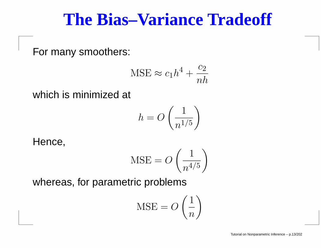
For many smoothers:
MSE ≈ c1h4 +
c2nh
which is minimized at
h = O
(1
n1/5
)
Hence,
MSE = O
(1
n4/5
)
whereas, for parametric problems
MSE = O
(1
n
)
Tutorial on Nonparametric Inference – p.13/202
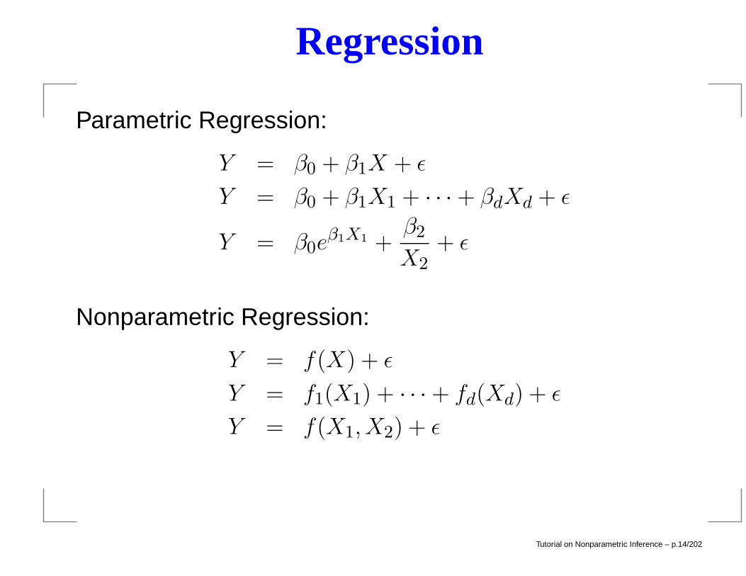
Regression
Parametric Regression:
Y = β0 + β1X + ε
Y = β0 + β1X1 + · · · + βdXd + ε
Y = β0eβ1X1 +
β2
X2+ ε
Nonparametric Regression:
Y = f(X) + ε
Y = f1(X1) + · · · + fd(Xd) + ε
Y = f(X1, X2) + ε
Tutorial on Nonparametric Inference – p.14/202
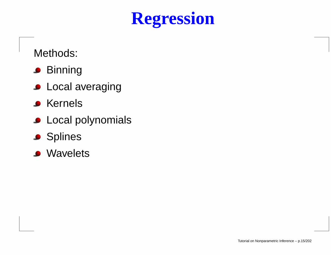
Regression
Methods:
Binning
Local averaging
Kernels
Local polynomials
Splines
Wavelets
Tutorial on Nonparametric Inference – p.15/202
Regression
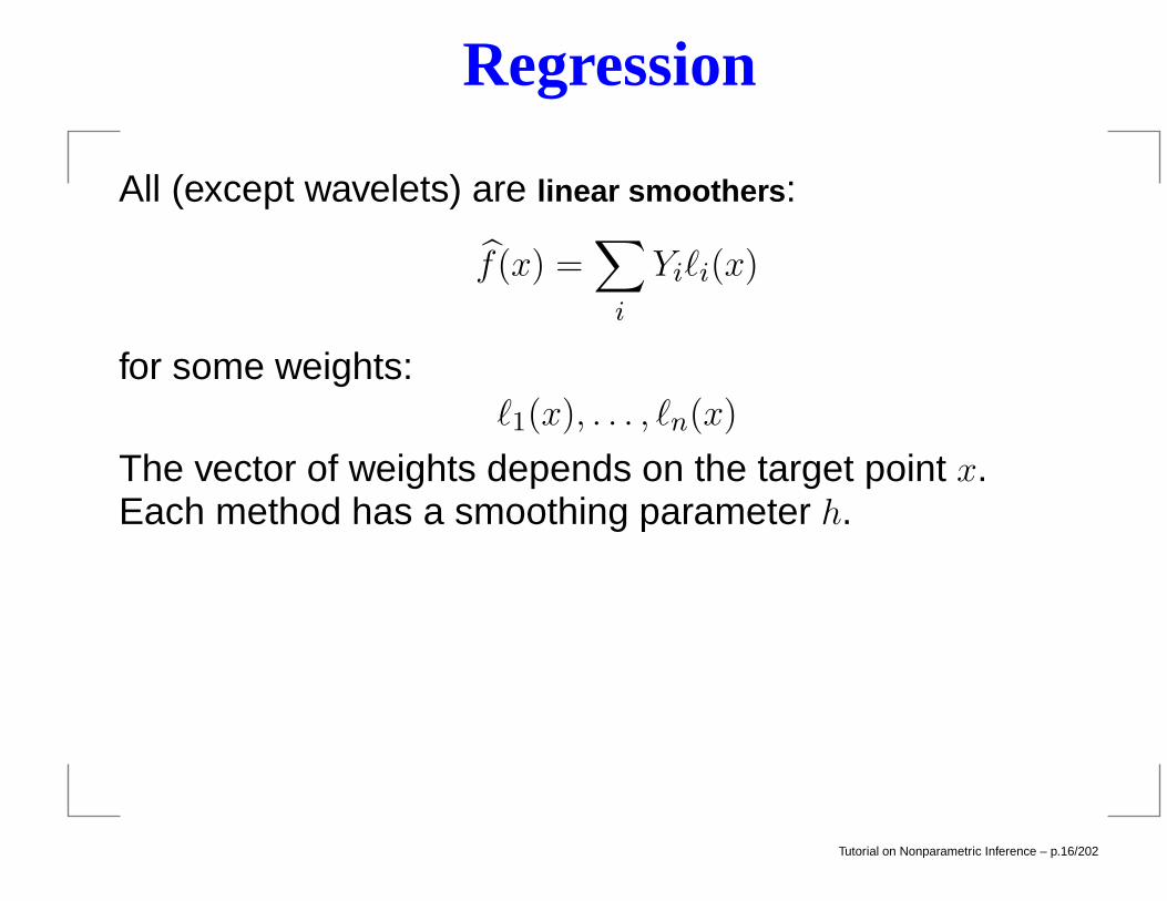
All (except wavelets) are linear smoothers:
f(x) =∑
i
Yi`i(x)
for some weights:`1(x), . . . , `n(x)
The vector of weights depends on the target point x.Each method has a smoothing parameter h.
Tutorial on Nonparametric Inference – p.16/202
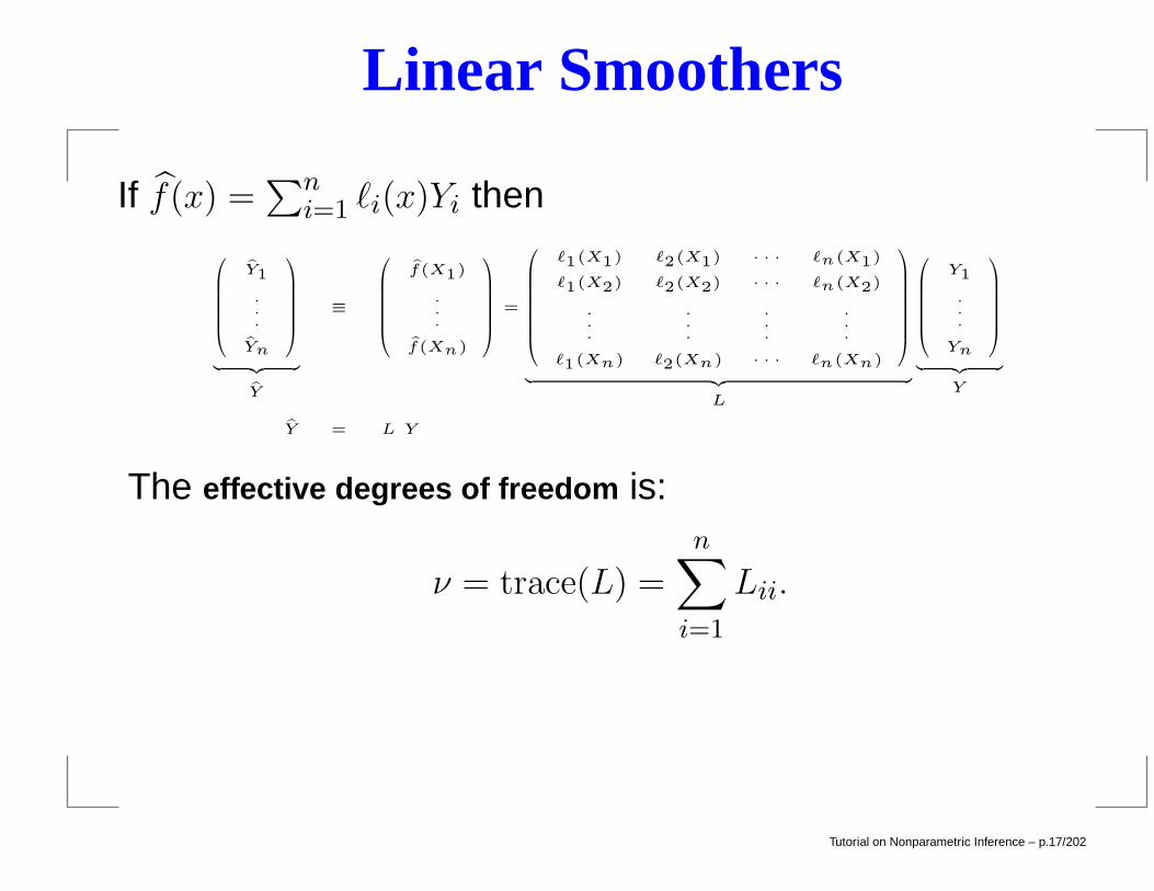
Linear Smoothers
If f(x) =∑n
i=1 `i(x)Yi then
Y1
.
.
.
Yn
︸ ︷︷ ︸Y
≡
f(X1)
.
.
.
f(Xn)
=
`1(X1) `2(X1) · · · `n(X1)
`1(X2) `2(X2) · · · `n(X2)
.
.
.
.
.
.
.
.
.
.
.
.
`1(Xn) `2(Xn) · · · `n(Xn)
︸ ︷︷ ︸L
Y1
.
.
.
Yn
︸ ︷︷ ︸Y
Y = L Y
The effective degrees of freedom is:
ν = trace(L) =
n∑
i=1
Lii.
Tutorial on Nonparametric Inference – p.17/202
Binning
Divide the x-axis into bins B1, B2, . . . of width h. f is a stepfunction based on averaging the Yi’s in each bin:
for x ∈ Bj : f(x) = mean
Yi : Xi ∈ Bj
.
The (arbitrary) choice of the boundaries of the bins canaffect inference, especially when h large.
Tutorial on Nonparametric Inference – p.18/202
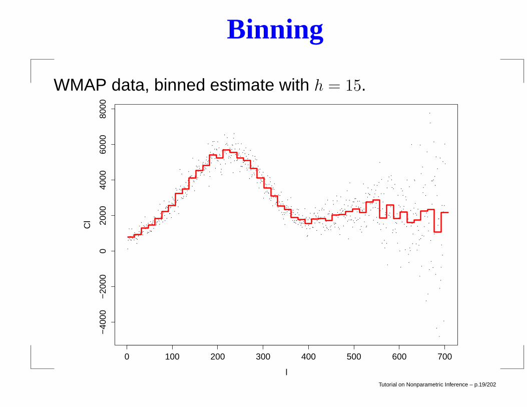
Binning
WMAP data, binned estimate with h = 15.
0 100 200 300 400 500 600 700
−40
00−
2000
020
0040
0060
0080
00
l
Cl
Tutorial on Nonparametric Inference – p.19/202

Binning
WMAP data, binned estimate with h = 50.
0 100 200 300 400 500 600 700
−40
00−
2000
020
0040
0060
0080
00
l
Cl
Tutorial on Nonparametric Inference – p.20/202
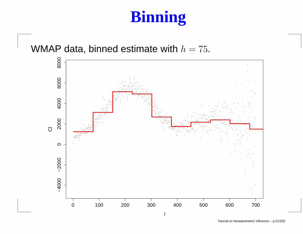
Binning
WMAP data, binned estimate with h = 75.
0 100 200 300 400 500 600 700
−40
00−
2000
020
0040
0060
0080
00
l
Cl
Tutorial on Nonparametric Inference – p.21/202
Local Averaging
For each x let
Nx =
[x− h
2, x+
h
2
].
This is a moving window of length h, centered at x. Define
f(x) = mean
Yi : Xi ∈ Nx
.
This is like binning but removes the arbitrary boundaries.
Tutorial on Nonparametric Inference – p.22/202
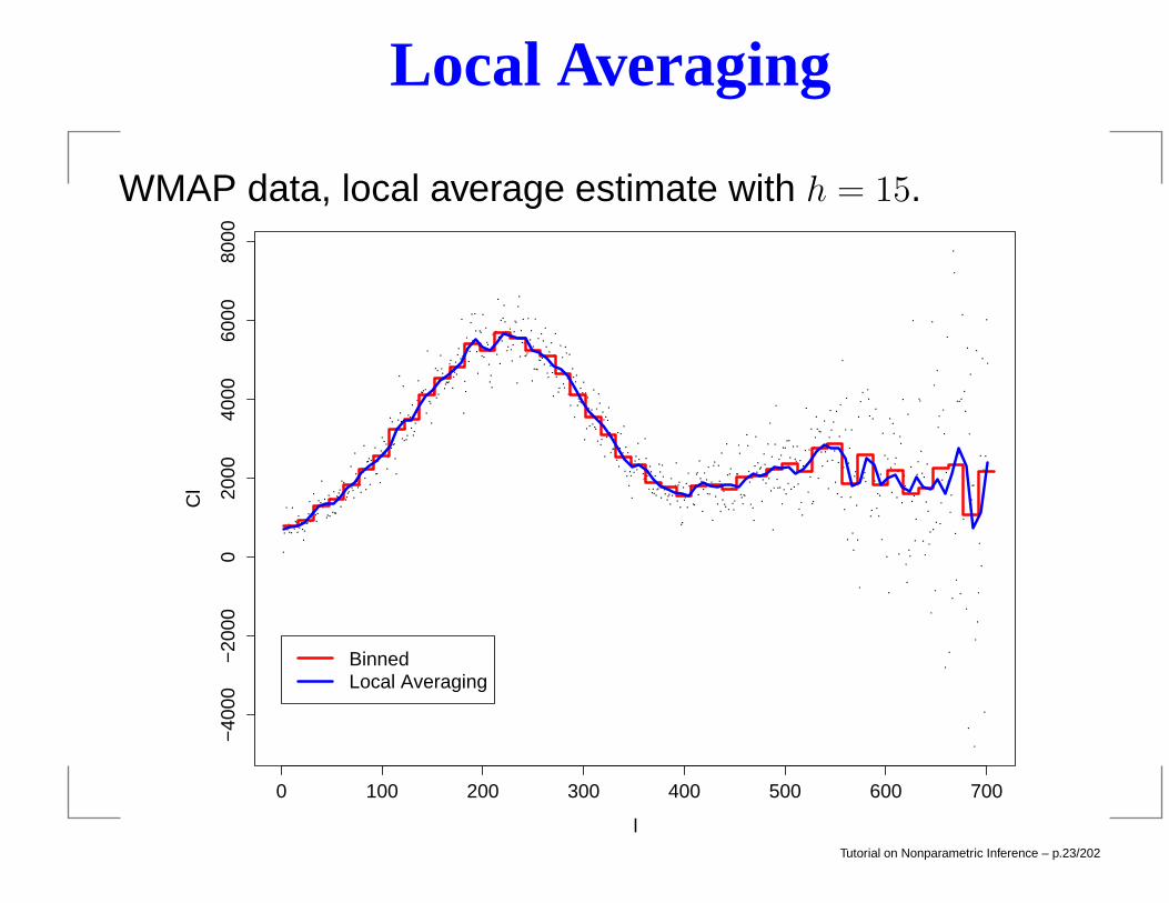
Local Averaging
WMAP data, local average estimate with h = 15.
0 100 200 300 400 500 600 700
−40
00−
2000
020
0040
0060
0080
00
l
Cl
BinnedLocal Averaging
Tutorial on Nonparametric Inference – p.23/202
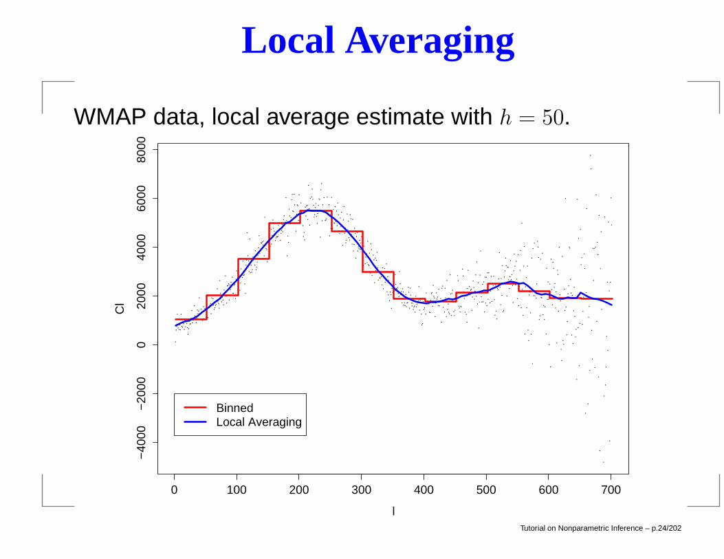
Local Averaging
WMAP data, local average estimate with h = 50.
0 100 200 300 400 500 600 700
−40
00−
2000
020
0040
0060
0080
00
l
Cl
BinnedLocal Averaging
Tutorial on Nonparametric Inference – p.24/202
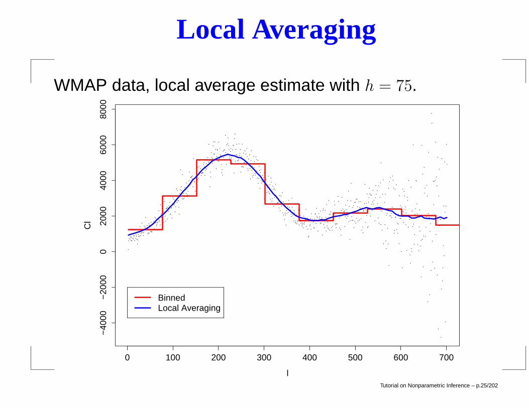
Local Averaging
WMAP data, local average estimate with h = 75.
0 100 200 300 400 500 600 700
−40
00−
2000
020
0040
0060
0080
00
l
Cl
BinnedLocal Averaging
Tutorial on Nonparametric Inference – p.25/202
Kernel Regression
The local average estimator can be written:
f(x) =
∑ni=1 Yi K
(x−Xi
h
)∑n
i=1K(x−Xi
h
)
where
K(x) =
1 |x| < 1/2
0 otherwise.
Can improve this by using a function K which is smoother.
Tutorial on Nonparametric Inference – p.26/202
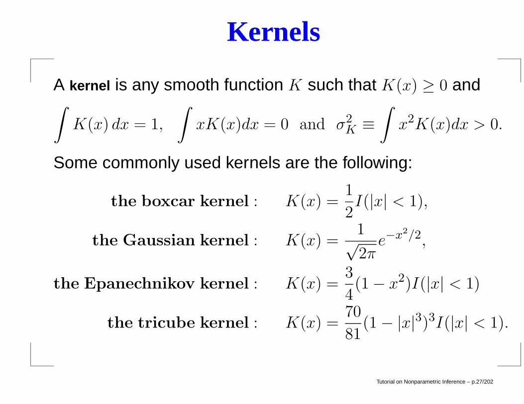
Kernels
A kernel is any smooth function K such that K(x) ≥ 0 and∫K(x) dx = 1,
∫xK(x)dx = 0 and σ2
K ≡∫x2K(x)dx > 0.
Some commonly used kernels are the following:
the boxcar kernel : K(x) =1
2I(|x| < 1),
the Gaussian kernel : K(x) =1√2πe−x
2/2,
the Epanechnikov kernel : K(x) =3
4(1− x2)I(|x| < 1)
the tricube kernel : K(x) =70
81(1− |x|3)3I(|x| < 1).
Tutorial on Nonparametric Inference – p.27/202
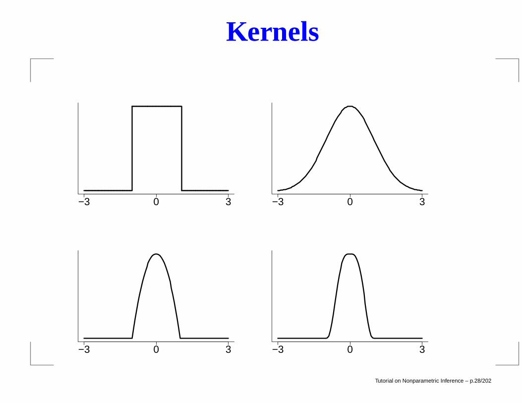
Kernels
−3 0 3 −3 0 3
−3 0 3 −3 0 3
Tutorial on Nonparametric Inference – p.28/202
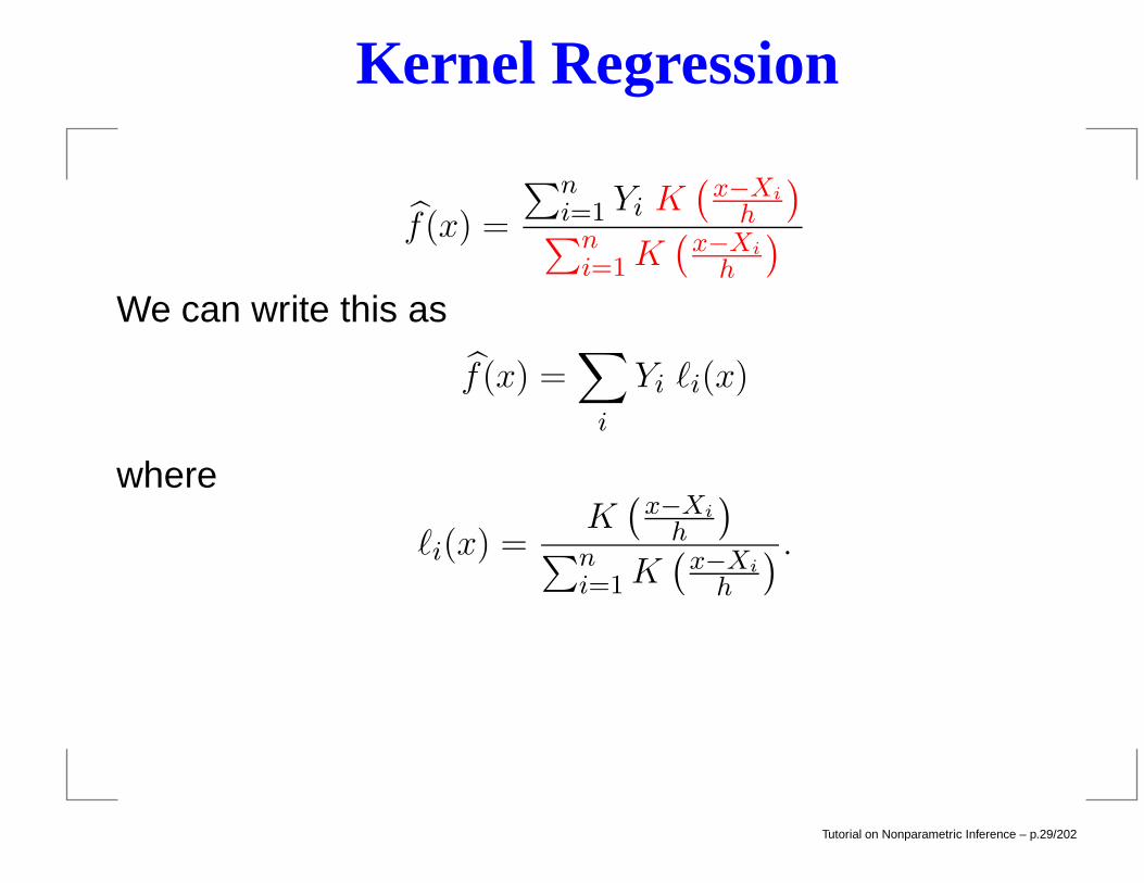
Kernel Regression
f(x) =
∑ni=1 Yi K
(x−Xi
h
)∑n
i=1K(x−Xi
h
)
We can write this as
f(x) =∑
i
Yi `i(x)
where
`i(x) =K(x−Xi
h
)∑n
i=1K(x−Xi
h
) .
Tutorial on Nonparametric Inference – p.29/202
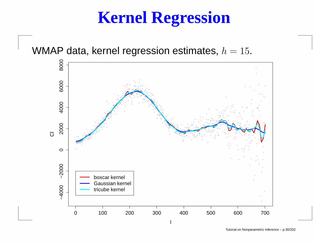
Kernel Regression
WMAP data, kernel regression estimates, h = 15.
0 100 200 300 400 500 600 700
−40
00−
2000
020
0040
0060
0080
00
l
Cl
boxcar kernelGaussian kerneltricube kernel
Tutorial on Nonparametric Inference – p.30/202
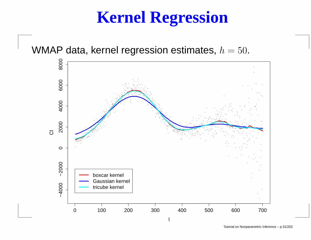
Kernel Regression
WMAP data, kernel regression estimates, h = 50.
0 100 200 300 400 500 600 700
−40
00−
2000
020
0040
0060
0080
00
l
Cl
boxcar kernelGaussian kerneltricube kernel
Tutorial on Nonparametric Inference – p.31/202
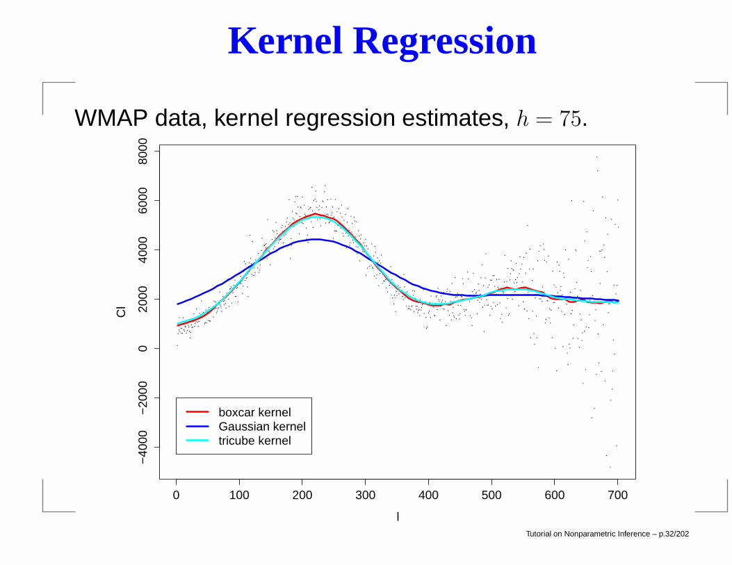
Kernel Regression
WMAP data, kernel regression estimates, h = 75.
0 100 200 300 400 500 600 700
−40
00−
2000
020
0040
0060
0080
00
l
Cl
boxcar kernelGaussian kerneltricube kernel
Tutorial on Nonparametric Inference – p.32/202
Kernel Regression
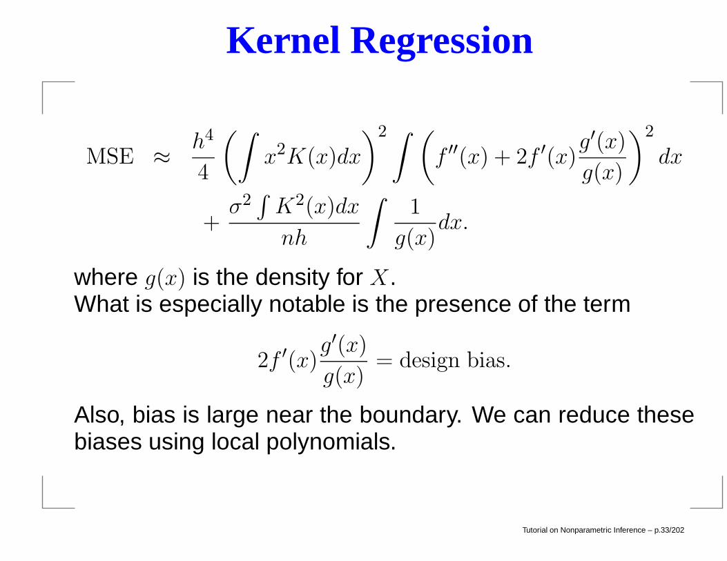
MSE ≈ h4
4
(∫x2K(x)dx
)2 ∫ (f ′′(x) + 2f ′(x)
g′(x)
g(x)
)2
dx
+σ2∫K2(x)dx
nh
∫1
g(x)dx.
where g(x) is the density for X.What is especially notable is the presence of the term
2f ′(x)g′(x)
g(x)= design bias.
Also, bias is large near the boundary. We can reduce thesebiases using local polynomials.
Tutorial on Nonparametric Inference – p.33/202
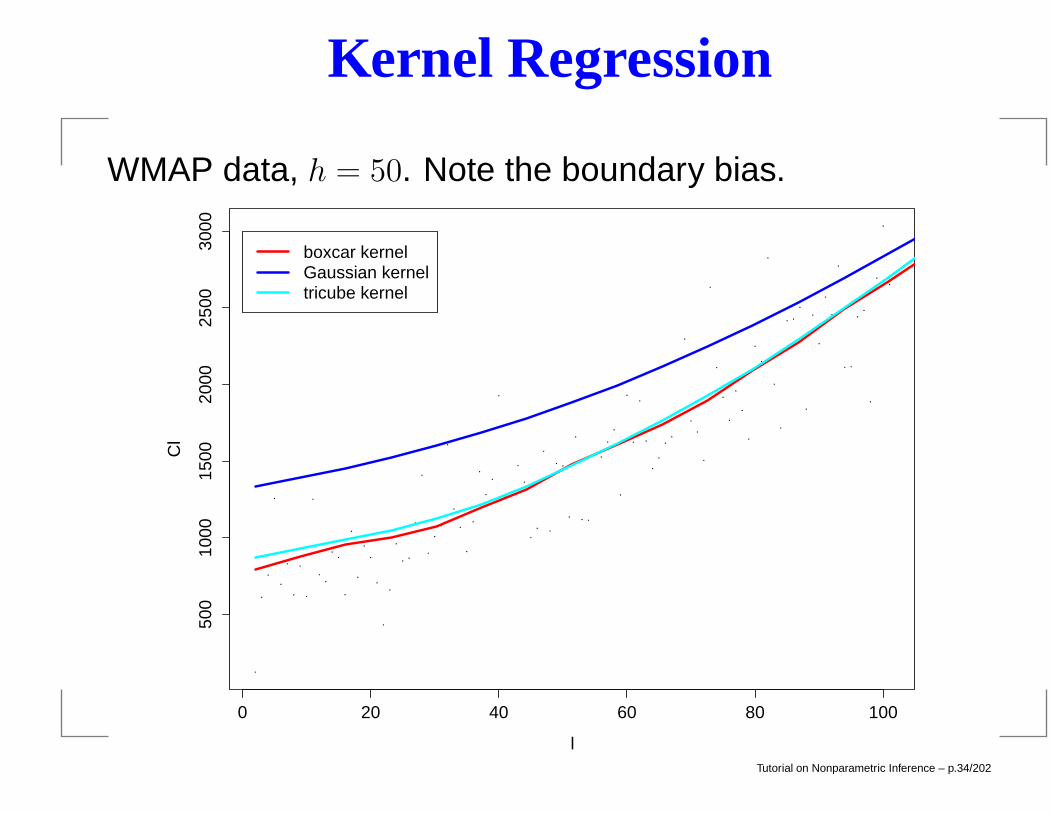
Kernel Regression
WMAP data, h = 50. Note the boundary bias.
0 20 40 60 80 100
500
1000
1500
2000
2500
3000
l
Cl
boxcar kernelGaussian kerneltricube kernel
Tutorial on Nonparametric Inference – p.34/202

Local Polynomial Regression
Recall polynomial regression:
f(x) = β0 + β1x+ β2x2 + · · · + βpx
p
where β = (β0, . . . , βp) are obtained by least squares:
minimize
n∑
i=1
(Yi − [β0 + β1x+ β2x
2 + · · ·+ βpxp]
)2
Tutorial on Nonparametric Inference – p.35/202
Local Polynomial Regression
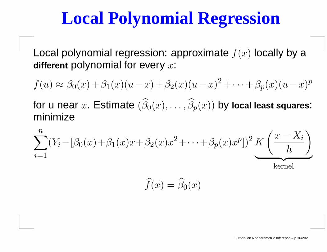
Local polynomial regression: approximate f(x) locally by adifferent polynomial for every x:
f(u) ≈ β0(x)+β1(x)(u−x)+β2(x)(u−x)2 + · · ·+βp(x)(u−x)p
for u near x. Estimate (β0(x), . . . , βp(x)) by local least squares:minimizen∑
i=1
(Yi−[β0(x)+β1(x)x+β2(x)x2+· · ·+βp(x)xp])2K
(x−Xi
h
)
︸ ︷︷ ︸kernel
f(x) = β0(x)
Tutorial on Nonparametric Inference – p.36/202
Local Polynomial Regression
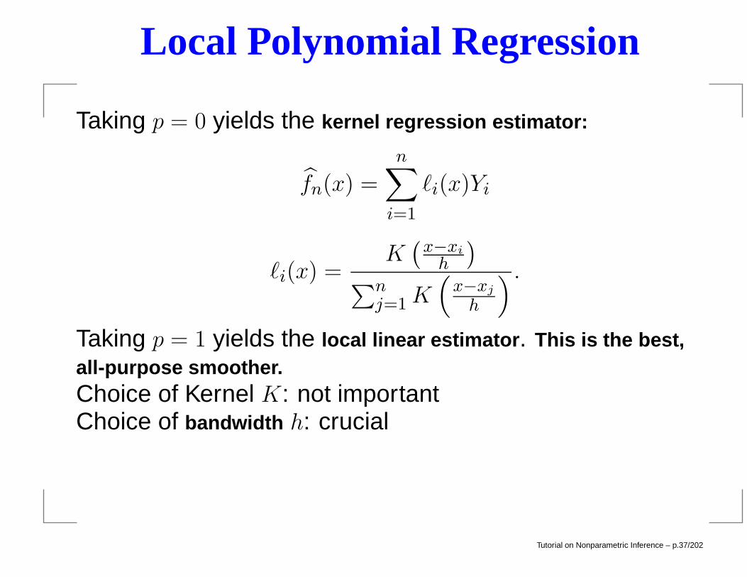
Taking p = 0 yields the kernel regression estimator:
fn(x) =
n∑
i=1
`i(x)Yi
`i(x) =K(x−xi
h
)∑n
j=1K(x−xj
h
) .
Taking p = 1 yields the local linear estimator. This is the best,all-purpose smoother.Choice of Kernel K: not importantChoice of bandwidth h: crucial
Tutorial on Nonparametric Inference – p.37/202
Local Polynomial Regression
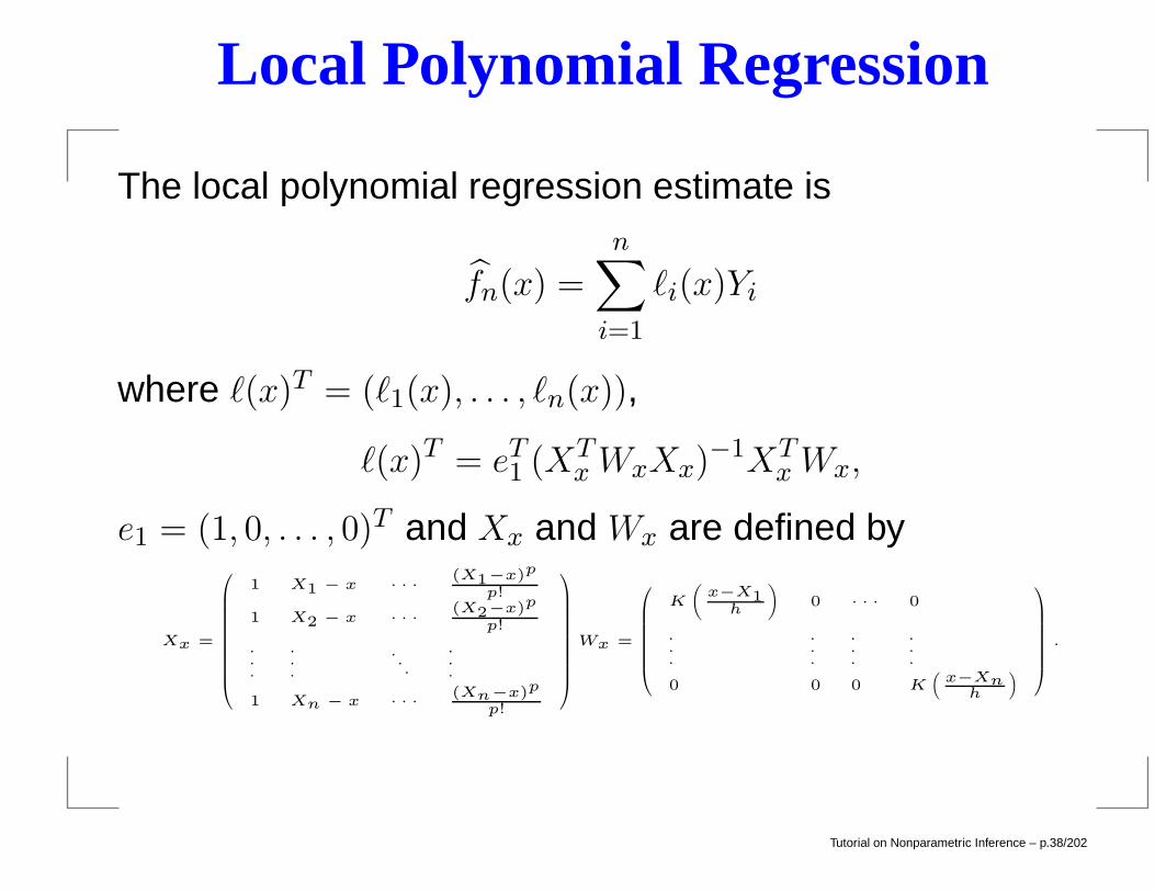
The local polynomial regression estimate is
fn(x) =
n∑
i=1
`i(x)Yi
where `(x)T = (`1(x), . . . , `n(x)),
`(x)T = eT1 (XTxWxXx)
−1XTxWx,
e1 = (1, 0, . . . , 0)T and Xx and Wx are defined by
Xx =
1 X1 − x · · ·(X1−x)p
p!
1 X2 − x · · ·(X2−x)p
p!
.
.
.
.
.
....
.
.
.
1 Xn − x · · ·(Xn−x)p
p!
Wx =
K
(x−X1
h
)0 · · · 0
.
.
.
.
.
.
.
.
.
.
.
.
0 0 0 K(
x−Xnh
)
.
Tutorial on Nonparametric Inference – p.38/202
Local Polynomial Regression
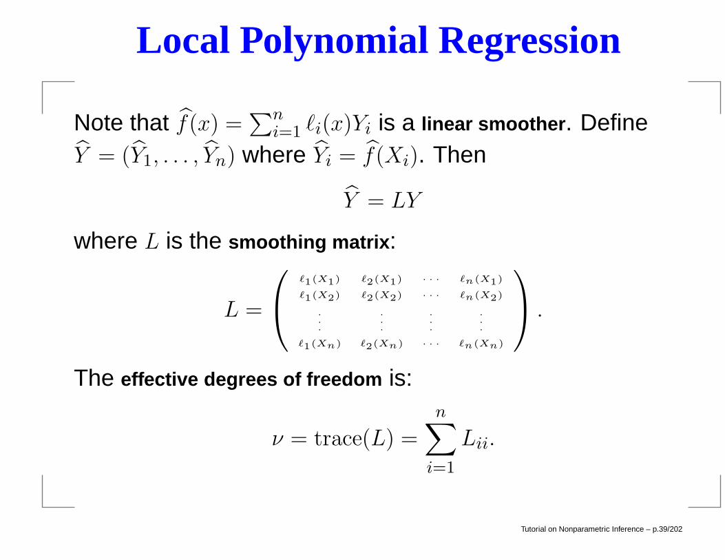
Note that f(x) =∑n
i=1 `i(x)Yi is a linear smoother. DefineY = (Y1, . . . , Yn) where Yi = f(Xi). Then
Y = LY
where L is the smoothing matrix:
L =
`1(X1) `2(X1) · · · `n(X1)
`1(X2) `2(X2) · · · `n(X2)
.
.
.
.
.
.
.
.
.
.
.
.
`1(Xn) `2(Xn) · · · `n(Xn)
.
The effective degrees of freedom is:
ν = trace(L) =n∑
i=1
Lii.
Tutorial on Nonparametric Inference – p.39/202
Choosing the Bandwidth
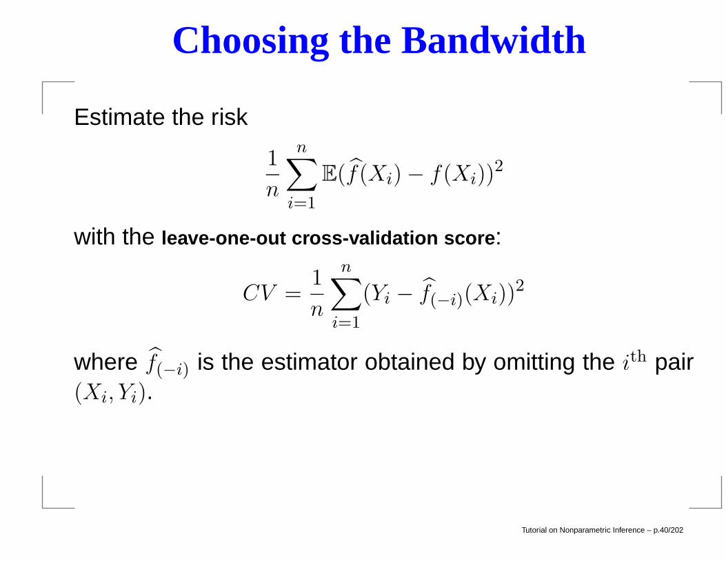
Estimate the risk
1
n
n∑
i=1
E(f(Xi)− f(Xi))2
with the leave-one-out cross-validation score:
CV =1
n
n∑
i=1
(Yi − f(−i)(Xi))2
where f(−i) is the estimator obtained by omitting the ith pair(Xi, Yi).
Tutorial on Nonparametric Inference – p.40/202
Choosing the Bandwidth
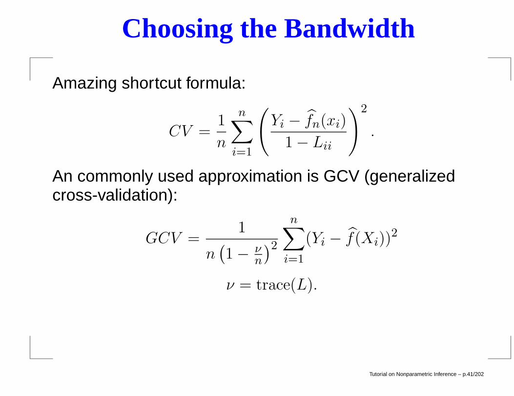
Amazing shortcut formula:
CV =1
n
n∑
i=1
(Yi − fn(xi)
1− Lii
)2
.
An commonly used approximation is GCV (generalizedcross-validation):
GCV =1
n(1− ν
n
)2n∑
i=1
(Yi − f(Xi))2
ν = trace(L).
Tutorial on Nonparametric Inference – p.41/202
Theoretical Aside
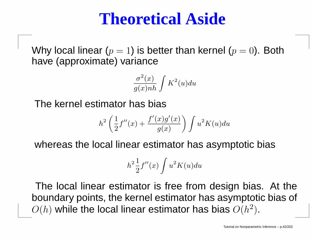
Why local linear (p = 1) is better than kernel (p = 0). Bothhave (approximate) variance
σ2(x)
g(x)nh
∫K2(u)du
The kernel estimator has bias
h2
(1
2f ′′(x) +
f ′(x)g′(x)
g(x)
)∫u2K(u)du
whereas the local linear estimator has asymptotic bias
h2 1
2f ′′(x)
∫u2K(u)du
The local linear estimator is free from design bias. At theboundary points, the kernel estimator has asymptotic bias ofO(h) while the local linear estimator has bias O(h2).
Tutorial on Nonparametric Inference – p.42/202
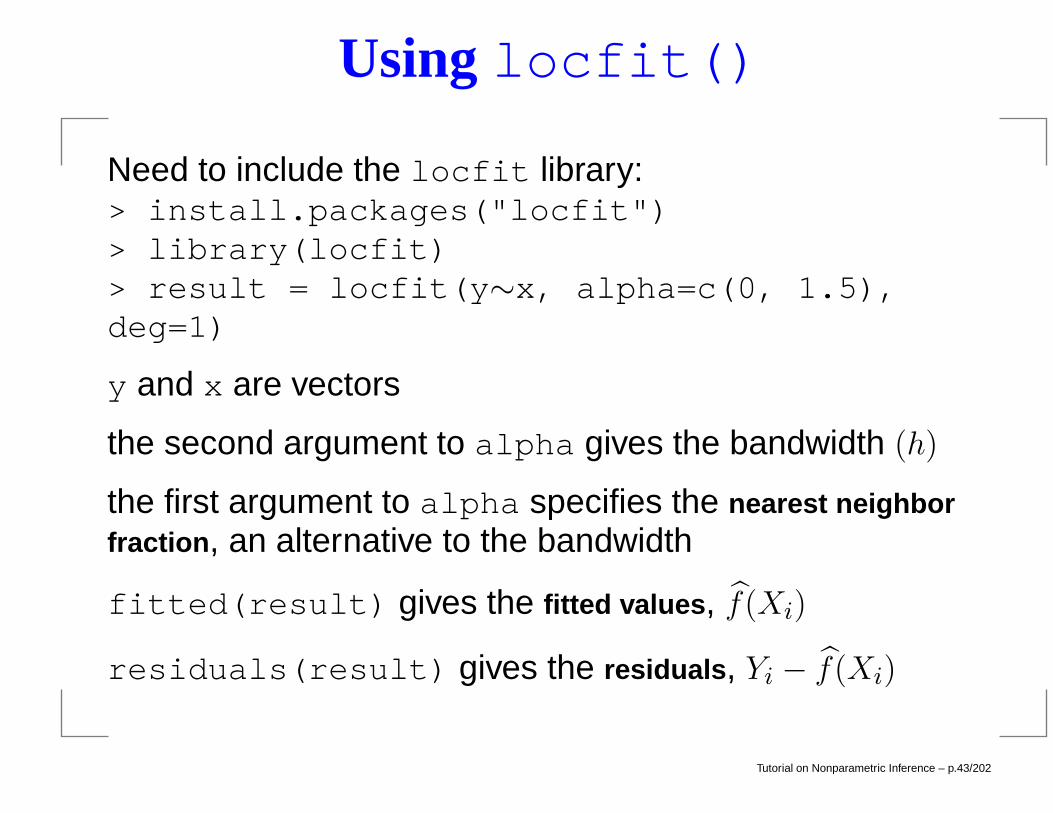
Using locfit()
Need to include the locfit library:> install.packages("locfit")> library(locfit)> result = locfit(y∼x, alpha=c(0, 1.5),deg=1)
y and x are vectors
the second argument to alpha gives the bandwidth (h)
the first argument to alpha specifies the nearest neighborfraction, an alternative to the bandwidth
fitted(result) gives the fitted values, f(Xi)
residuals(result) gives the residuals, Yi − f(Xi)
Tutorial on Nonparametric Inference – p.43/202
Using locfit()
See the R code locfit R example, the functionlocfit simdata().
Allows specification the true function f(x), simulate dataYi = f(Xi) + εi, i = 1, 2, . . . , n, where εi is normal(0,σ).
Illustrates the use of the function gcvplot(), which calcu-lates GCV for specified bandwidths.
Tutorial on Nonparametric Inference – p.44/202
An Aside: Functions in R
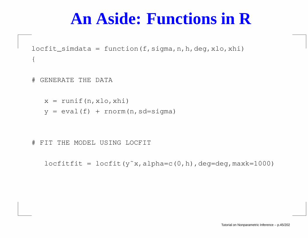
locfit_simdata = function(f,sigma,n,h,deg,xlo,xhi)
# GENERATE THE DATA
x = runif(n,xlo,xhi)
y = eval(f) + rnorm(n,sd=sigma)
# FIT THE MODEL USING LOCFIT
locfitfit = locfit(y˜x,alpha=c(0,h),deg=deg,maxk=1000)
Tutorial on Nonparametric Inference – p.45/202
An Aside: Functions in R
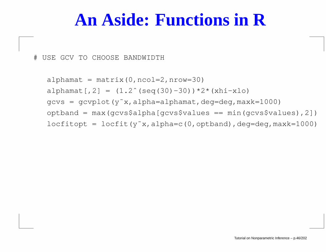
# USE GCV TO CHOOSE BANDWIDTH
alphamat = matrix(0,ncol=2,nrow=30)
alphamat[,2] = (1.2ˆ(seq(30)-30))*2*(xhi-xlo)
gcvs = gcvplot(y˜x,alpha=alphamat,deg=deg,maxk=1000)
optband = max(gcvs$alpha[gcvs$values == min(gcvs$values),2])
locfitopt = locfit(y˜x,alpha=c(0,optband),deg=deg,maxk=1000)
Tutorial on Nonparametric Inference – p.46/202
An Aside: Functions in R
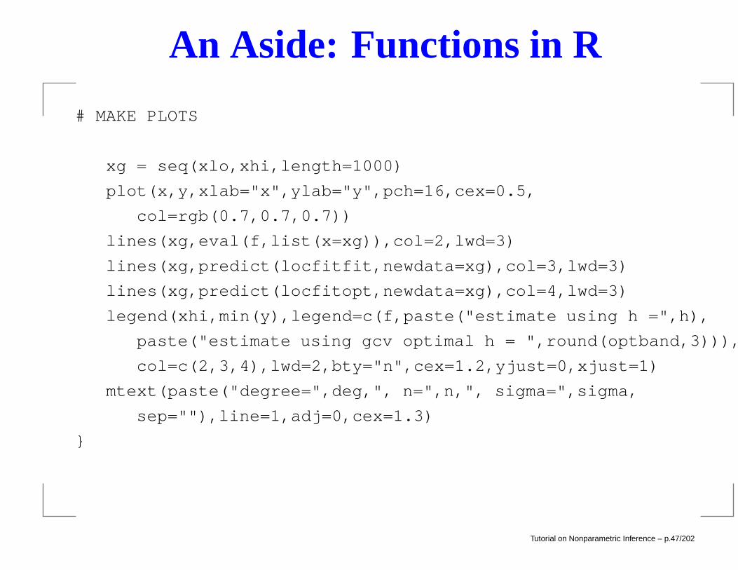
# MAKE PLOTS
xg = seq(xlo,xhi,length=1000)
plot(x,y,xlab="x",ylab="y",pch=16,cex=0.5,
col=rgb(0.7,0.7,0.7))
lines(xg,eval(f,list(x=xg)),col=2,lwd=3)
lines(xg,predict(locfitfit,newdata=xg),col=3,lwd=3)
lines(xg,predict(locfitopt,newdata=xg),col=4,lwd=3)
legend(xhi,min(y),legend=c(f,paste("estimate using h =",h),
paste("estimate using gcv optimal h = ",round(optband,3))),
col=c(2,3,4),lwd=2,bty="n",cex=1.2,yjust=0,xjust=1)
mtext(paste("degree=",deg,", n=",n,", sigma=",sigma,
sep=""),line=1,adj=0,cex=1.3)
Tutorial on Nonparametric Inference – p.47/202
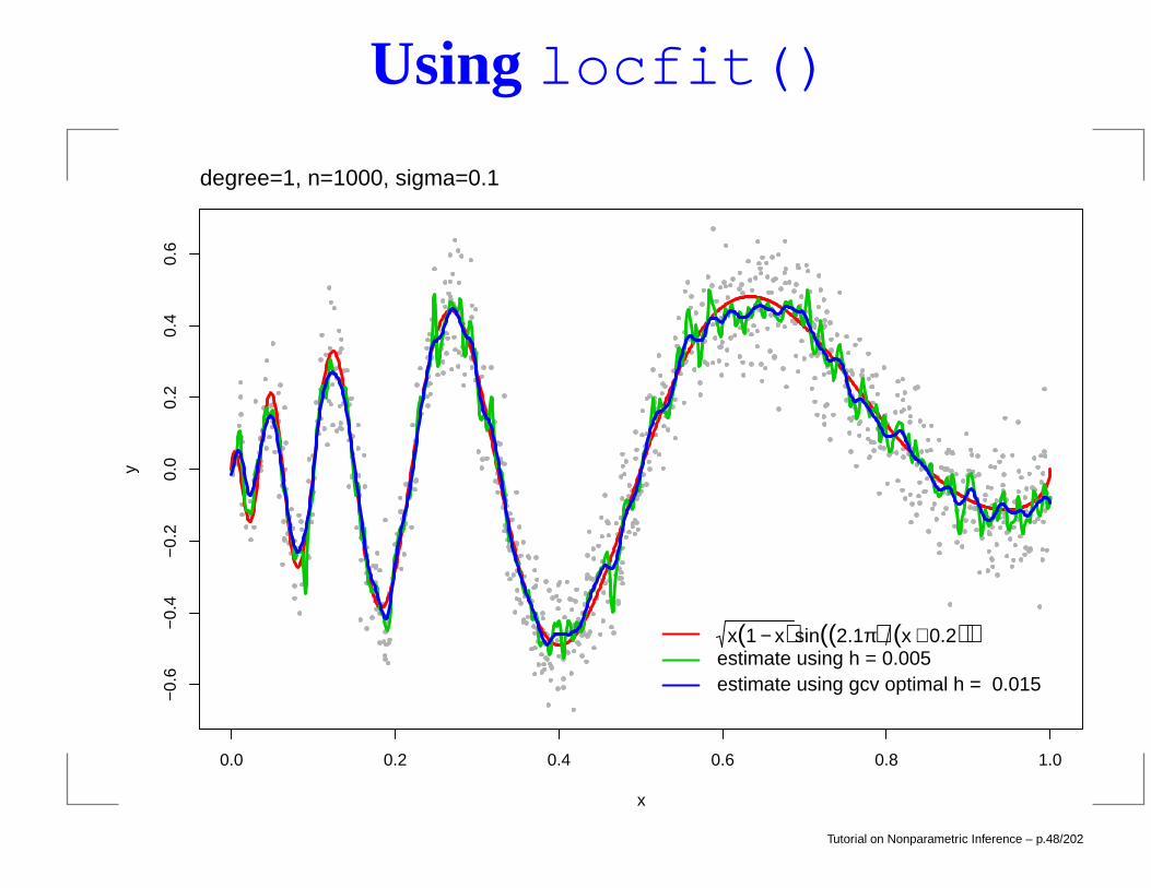
Using locfit()
0.0 0.2 0.4 0.6 0.8 1.0
−0.
6−
0.4
−0.
20.
00.
20.
40.
6
x
y
x(1 − x)sin((2.1π) (x + 0.2))estimate using h = 0.005estimate using gcv optimal h = 0.015
degree=1, n=1000, sigma=0.1
Tutorial on Nonparametric Inference – p.48/202
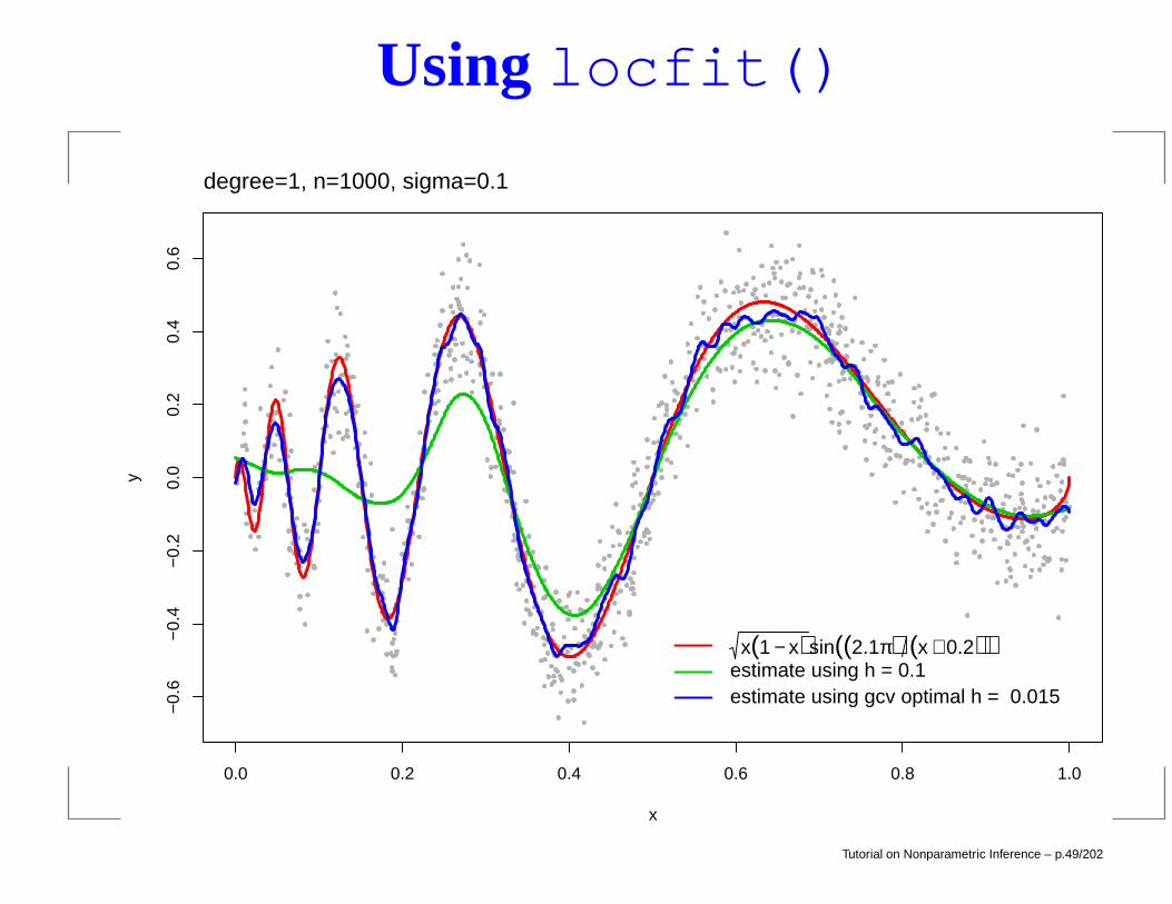
Using locfit()
0.0 0.2 0.4 0.6 0.8 1.0
−0.
6−
0.4
−0.
20.
00.
20.
40.
6
x
y
x(1 − x)sin((2.1π) (x + 0.2))estimate using h = 0.1estimate using gcv optimal h = 0.015
degree=1, n=1000, sigma=0.1
Tutorial on Nonparametric Inference – p.49/202
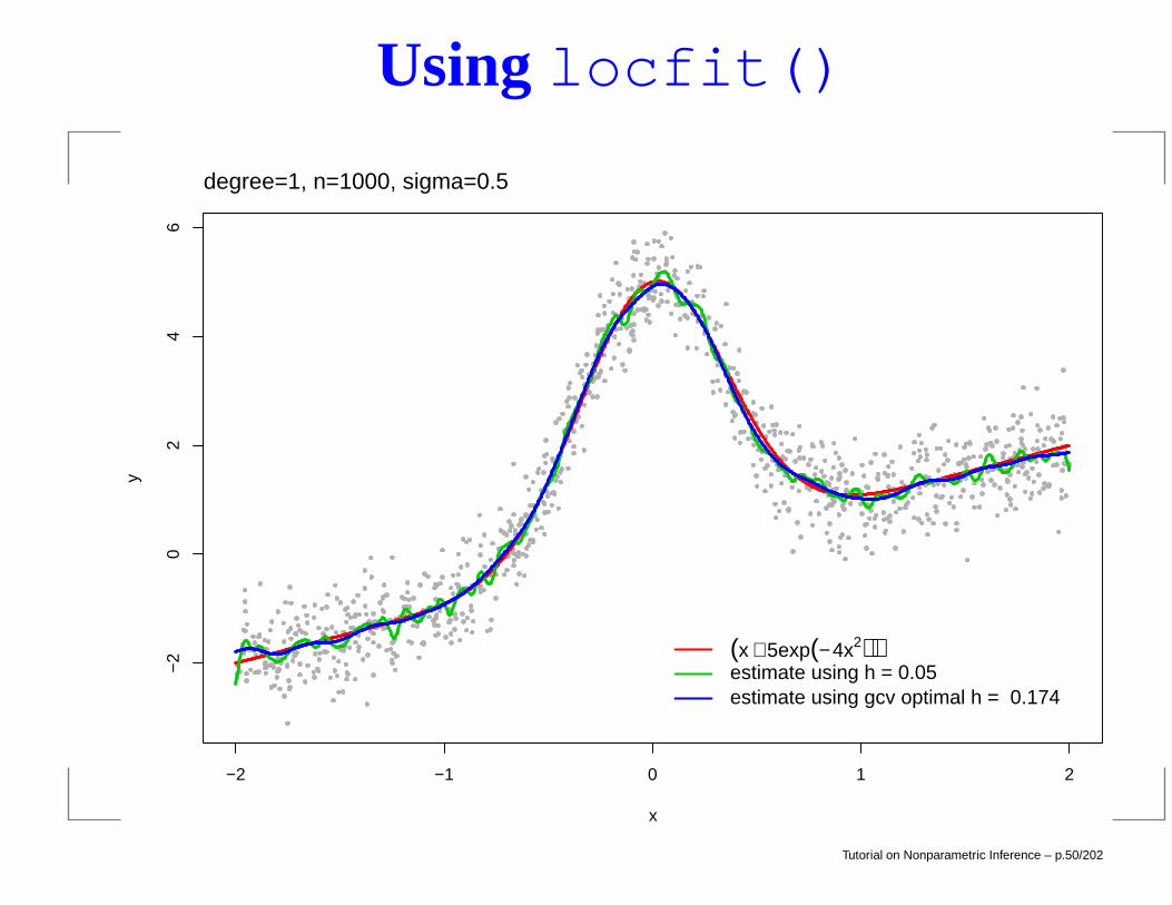
Using locfit()
−2 −1 0 1 2
−2
02
46
x
y
(x + 5exp(− 4x2))estimate using h = 0.05estimate using gcv optimal h = 0.174
degree=1, n=1000, sigma=0.5
Tutorial on Nonparametric Inference – p.50/202
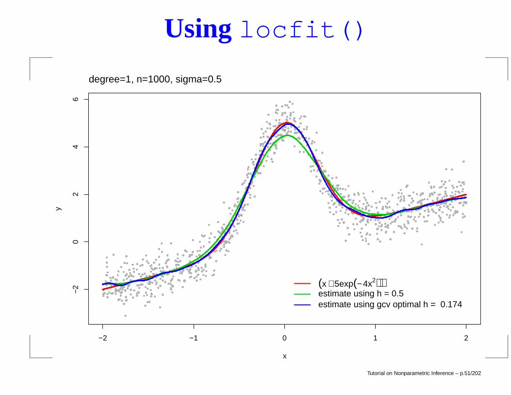
Using locfit()
−2 −1 0 1 2
−2
02
46
x
y
(x + 5exp(− 4x2))estimate using h = 0.5estimate using gcv optimal h = 0.174
degree=1, n=1000, sigma=0.5
Tutorial on Nonparametric Inference – p.51/202
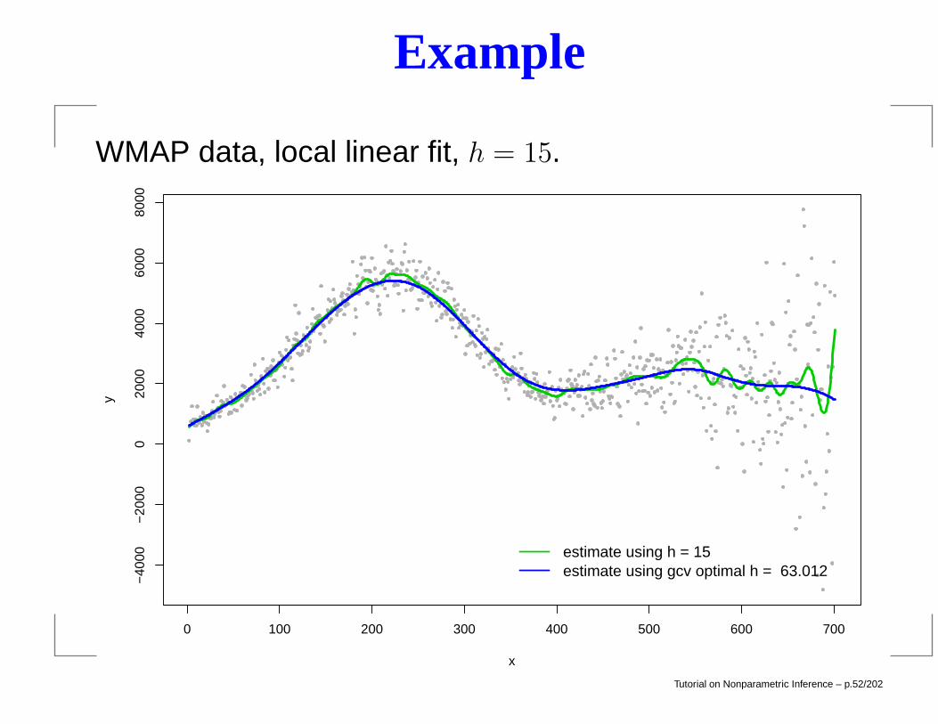
Example
WMAP data, local linear fit, h = 15.
0 100 200 300 400 500 600 700
−40
00−
2000
020
0040
0060
0080
00
x
y
estimate using h = 15estimate using gcv optimal h = 63.012
Tutorial on Nonparametric Inference – p.52/202
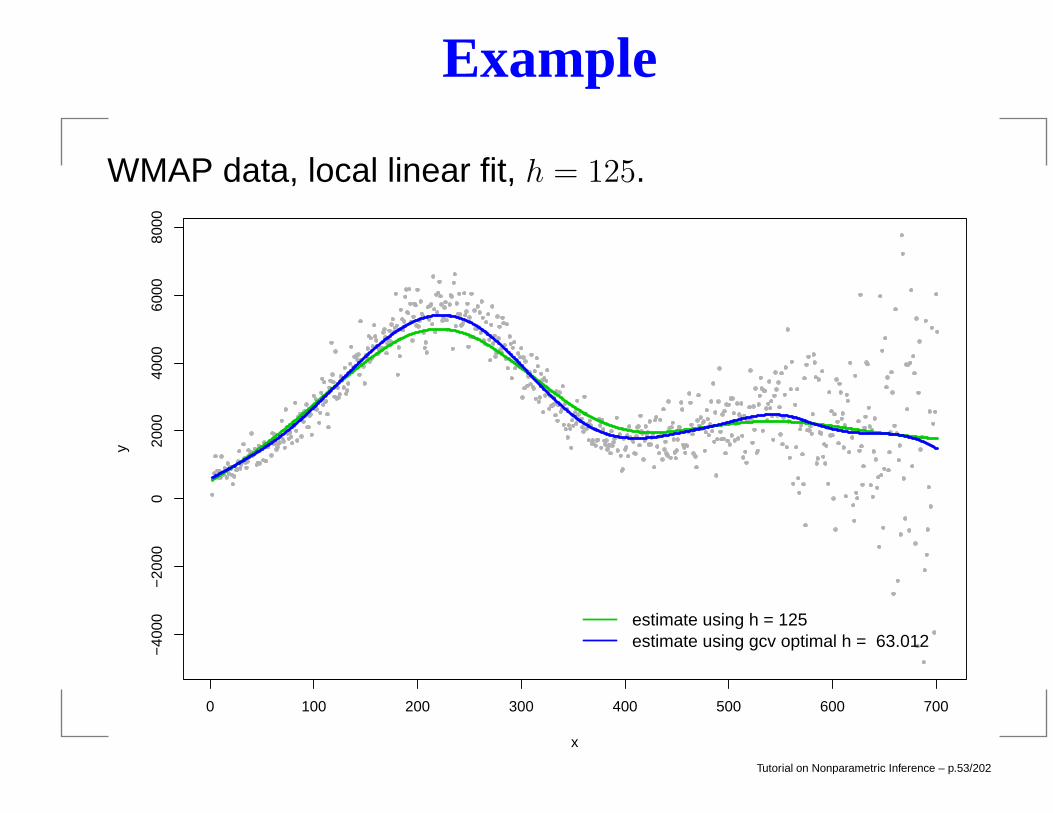
Example
WMAP data, local linear fit, h = 125.
0 100 200 300 400 500 600 700
−40
00−
2000
020
0040
0060
0080
00
x
y
estimate using h = 125estimate using gcv optimal h = 63.012
Tutorial on Nonparametric Inference – p.53/202
Variance Estimation
Let
σ2 =
∑ni=1(Yi − f(xi))
2
n− 2ν + ν
where
ν = tr(L), ν = tr(LTL) =n∑
i=1
||`(xi)||2.
If f is sufficiently smooth, then σ2 is a consistent estimatorof σ2.
Tutorial on Nonparametric Inference – p.54/202
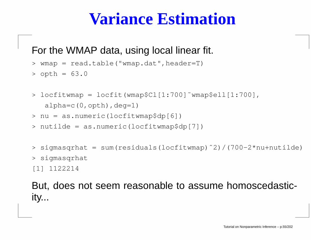
Variance Estimation
For the WMAP data, using local linear fit.> wmap = read.table("wmap.dat",header=T)
> opth = 63.0
> locfitwmap = locfit(wmap$Cl[1:700]˜wmap$ell[1:700],
alpha=c(0,opth),deg=1)
> nu = as.numeric(locfitwmap$dp[6])
> nutilde = as.numeric(locfitwmap$dp[7])
> sigmasqrhat = sum(residuals(locfitwmap)ˆ2)/(700-2*nu+nutilde)
> sigmasqrhat
[1] 1122214
But, does not seem reasonable to assume homoscedastic-ity...
Tutorial on Nonparametric Inference – p.55/202
Variance Estimation
Allow σ to be a function of x:
Yi = f(xi) + σ(xi)εi.
Let Zi = log(Yi − f(xi))2 and δi = log ε2i . Then,
Zi = log(σ2(xi)) + δi.
This suggests estimating log σ2(x) by regressing the logsquared residuals on x.
Tutorial on Nonparametric Inference – p.56/202
Variance Estimation
1. Estimate f(x) with any nonparametric method to get anestimate fn(x).
2. Define Zi = log(Yi − fn(xi))2.
3. Regress the Zi’s on the xi’s (again using anynonparametric method) to get an estimate q(x) oflog σ2(x) and let
σ2(x) = eq(x).
Tutorial on Nonparametric Inference – p.57/202
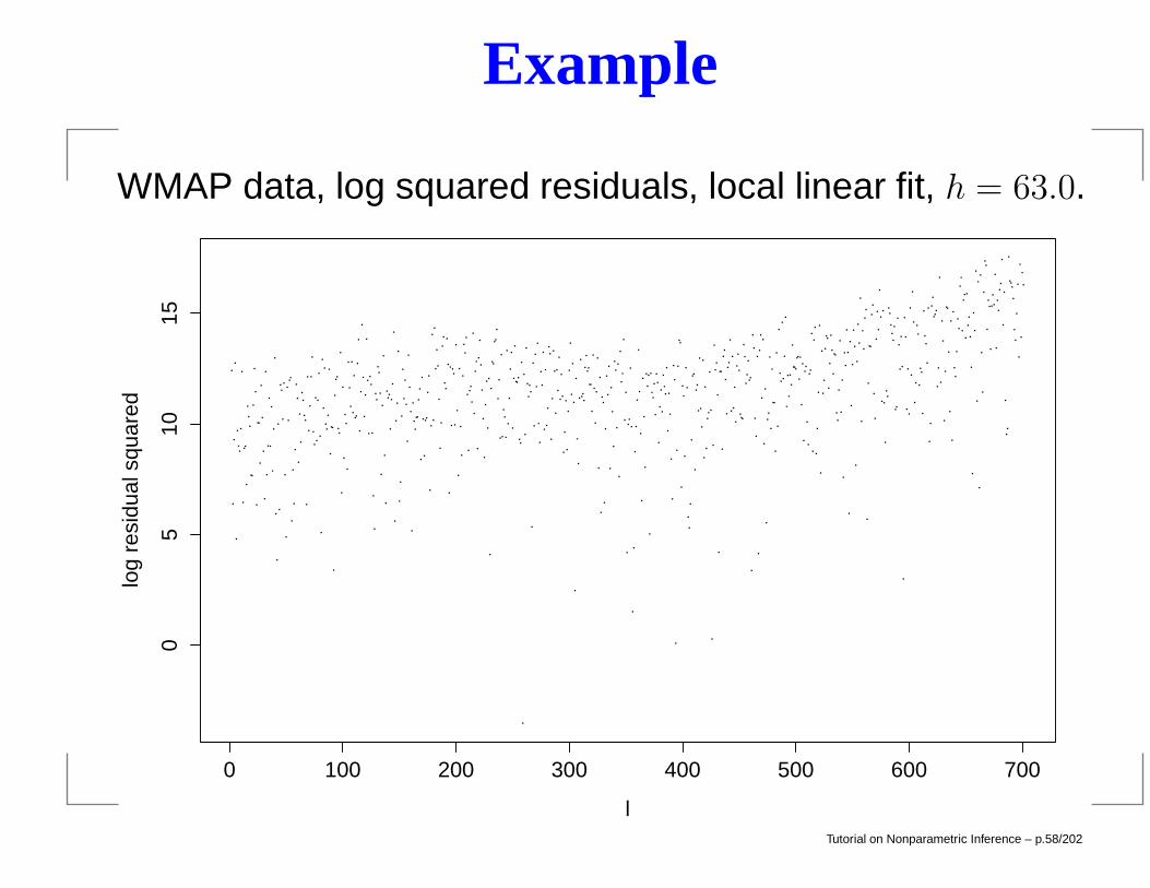
Example
WMAP data, log squared residuals, local linear fit, h = 63.0.
0 100 200 300 400 500 600 700
05
1015
l
log
resi
dual
squ
ared
Tutorial on Nonparametric Inference – p.58/202
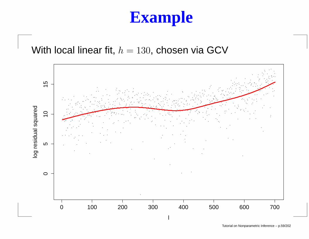
Example
With local linear fit, h = 130, chosen via GCV
0 100 200 300 400 500 600 700
05
1015
l
log
resi
dual
squ
ared
Tutorial on Nonparametric Inference – p.59/202
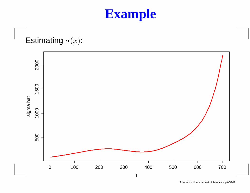
Example
Estimating σ(x):
0 100 200 300 400 500 600 700
500
1000
1500
2000
l
sigm
a ha
t
Tutorial on Nonparametric Inference – p.60/202
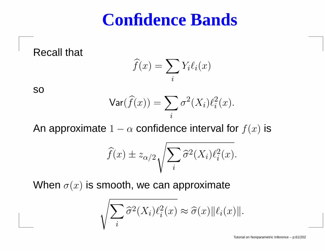
Confidence Bands
Recall thatf(x) =
∑
i
Yi`i(x)
soVar(f(x)) =
∑
i
σ2(Xi)`2i (x).
An approximate 1− α confidence interval for f(x) is
f(x)± zα/2√∑
i
σ2(Xi)`2i (x).
When σ(x) is smooth, we can approximate√∑
i
σ2(Xi)`2i (x) ≈ σ(x)‖`i(x)‖.
Tutorial on Nonparametric Inference – p.61/202
Confidence Bands
Two caveats:
1. f is biased so this is realy an interval for E(f(x)). Result:bands can miss sharp peaks in the function.
2. Pointwise coverage does not imply simultaneouscoverage for all x.
Solution for 2 is to replace zα/2 with a larger number (Sunand Loader 1994). locfit() does this for you.
Tutorial on Nonparametric Inference – p.62/202
More on locfit()
> diaghat = predict.locfit(locfitwmap,where="data",what="infl")
> normell = predict.locfit(locfitwmap,where="data",what="vari")
diaghat will be Lii, i = 1, 2, . . . , n.normell will be ‖`i(x)‖, i = 1, 2, . . . , n
The Sun and Loader replacement for zα/2 is found usingkappa0(locfitwmap)$crit.val.
Tutorial on Nonparametric Inference – p.63/202
More on locfit()
> critval = kappa0(locfitwmap)$crit.val
> postscript("confbandssimul.eps",width=10,height=7)
> plot(wmap$ell[1:700],fitwmap,lwd=3, xlab="l",ylab="Cl",
cex=3,cex.axis=1.3, cex.lab=1.3,type="l")
> lines(wmap$ell[1:700],fitwmap+
critval*sqrt(sigmasqrhat*normell),col=2,lwd=3)
> lines(wmap$ell[1:700],fitwmap-
critval*sqrt(sigmasqrhat*normell),col=2,lwd=3)
...
Tutorial on Nonparametric Inference – p.64/202
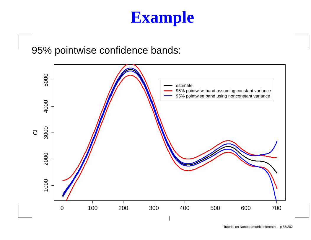
Example
95% pointwise confidence bands:
0 100 200 300 400 500 600 700
1000
2000
3000
4000
5000
l
Cl
estimate95% pointwise band assuming constant variance95% pointwise band using nonconstant variance
Tutorial on Nonparametric Inference – p.65/202
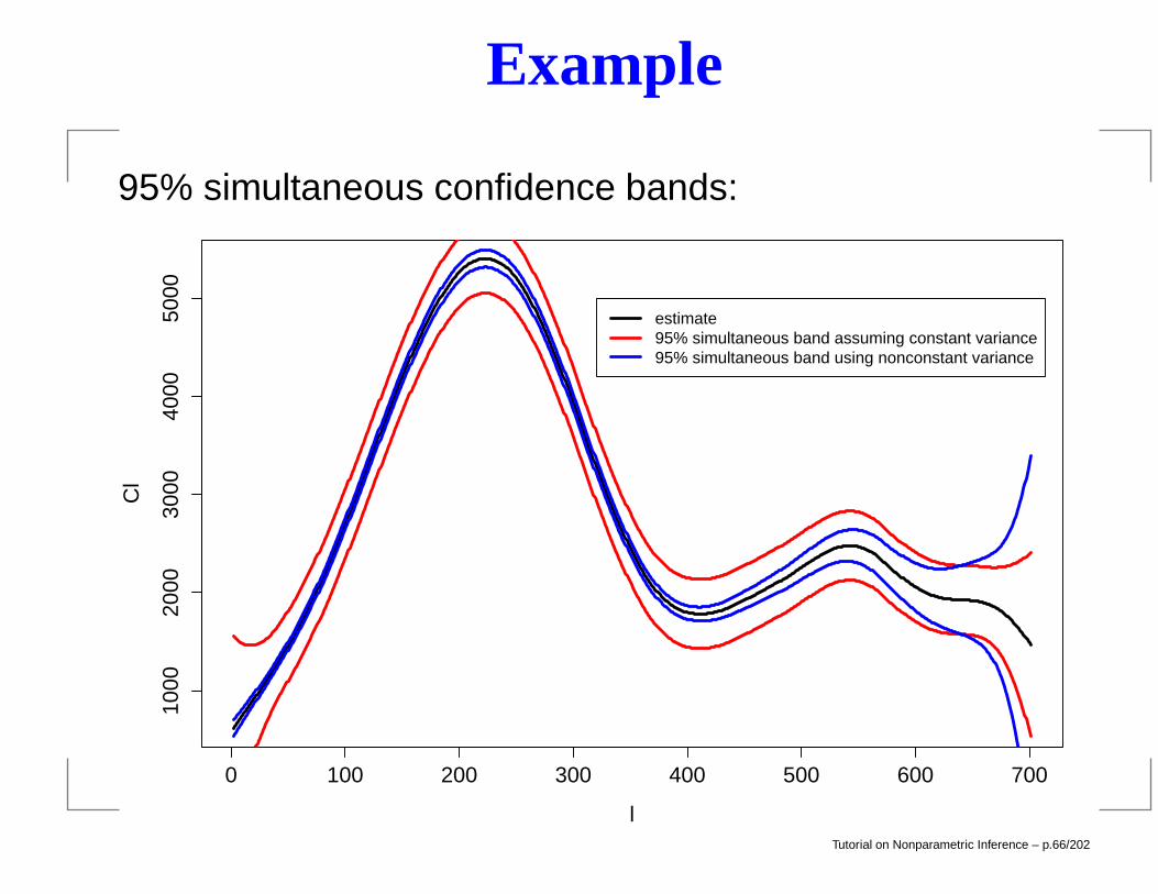
Example
95% simultaneous confidence bands:
0 100 200 300 400 500 600 700
1000
2000
3000
4000
5000
l
Cl
estimate95% simultaneous band assuming constant variance95% simultaneous band using nonconstant variance
Tutorial on Nonparametric Inference – p.66/202
Basis Methods
Idea: expand f as
f(x) =∑
j
βjψj(x)
where ψ1(x), ψ2(x), . . . are specially chosen, knownfunctions. Then estimate βj and set
f(x) =∑
j
βjψj(x).
We consider two versions: (i) splines, (ii) wavelets.
Tutorial on Nonparametric Inference – p.67/202
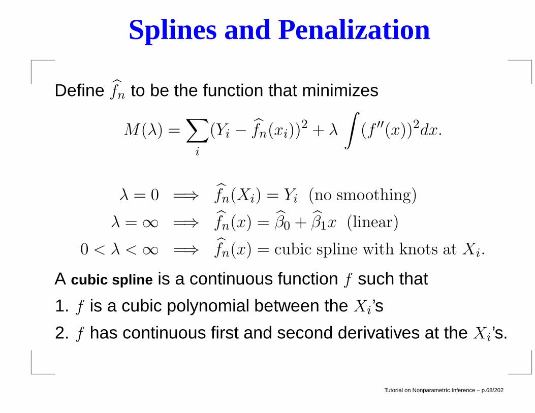
Splines and Penalization
Define fn to be the function that minimizes
M(λ) =∑
i
(Yi − fn(xi))2 + λ
∫(f ′′(x))2dx.
λ = 0 =⇒ fn(Xi) = Yi (no smoothing)
λ =∞ =⇒ fn(x) = β0 + β1x (linear)
0 < λ <∞ =⇒ fn(x) = cubic spline with knots at Xi.
A cubic spline is a continuous function f such that
1. f is a cubic polynomial between the Xi’s
2. f has continuous first and second derivatives at the Xi’s.
Tutorial on Nonparametric Inference – p.68/202
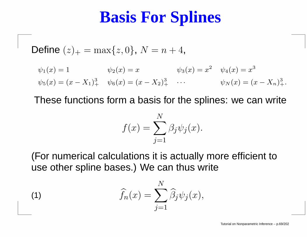
Basis For Splines
Define (z)+ = maxz, 0, N = n+ 4,
ψ1(x) = 1 ψ2(x) = x ψ3(x) = x2 ψ4(x) = x3
ψ5(x) = (x−X1)3+ ψ6(x) = (x−X2)
3+ · · · ψN (x) = (x−Xn)3+.
These functions form a basis for the splines: we can write
f(x) =N∑
j=1
βjψj(x).
(For numerical calculations it is actually more efficient touse other spline bases.) We can thus write
fn(x) =N∑
j=1
βjψj(x),(1)
Tutorial on Nonparametric Inference – p.69/202
Basis For Splines
We can now rewrite the minimization as follows:
minimize : (Y −Ψβ)T (Y −Ψβ) + λβTΩβ
where Ψij = ψj(Xi) and Ωjk =∫ψ′′j (x)ψ
′′k(x)dx. The value of
β that minimizes this is
β = (ΨTΨ + λΩ)−1ΨTY.
The smoothing spline fn(x) is a linear smoother, that is, thereexist weights `(x) such that fn(x) =
∑ni=1 Yi`i(x).
Tutorial on Nonparametric Inference – p.70/202
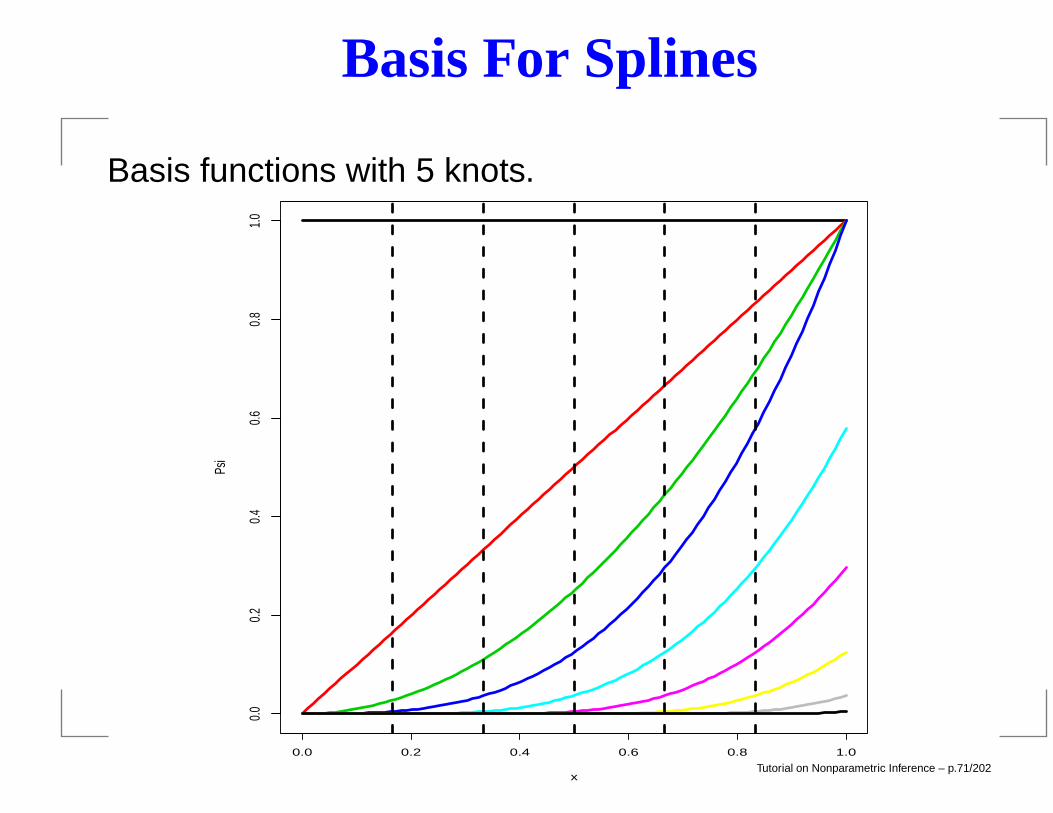
Basis For Splines
Basis functions with 5 knots.
0.0 0.2 0.4 0.6 0.8 1.0
0.0
0.2
0.4
0.6
0.8
1.0
x
Psi
Tutorial on Nonparametric Inference – p.71/202

Basis For Splines
Same span as previous slide, the B-spline basis, 5 knots:
0.0 0.2 0.4 0.6 0.8 1.0
0.0
0.2
0.4
0.6
0.8
1.0
x
Tutorial on Nonparametric Inference – p.72/202
Smoothing Splines in R
> smosplresult = spline.smooth(x,y,cv=FALSE, all.knots=TRUE)
If cv=TRUE, then cross-validiation used to choose λ; ifcv=FALSE, gcv is used
If all.knots=TRUE, then knots are placed at all datapoints; if all.knots=FALSE, then set nknots to specifythe number of knots to be used. Using fewer knots easesthe computational cost.
predict(smosplresult) gives fitted values.
Tutorial on Nonparametric Inference – p.73/202
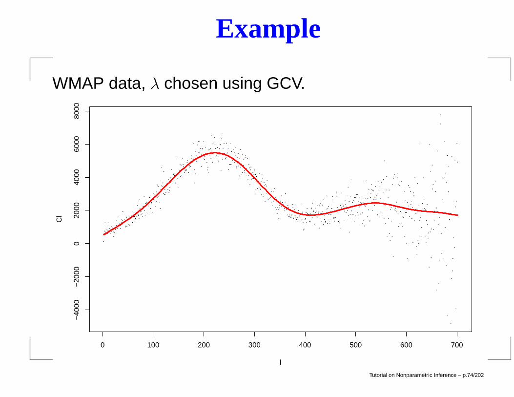
Example
WMAP data, λ chosen using GCV.
0 100 200 300 400 500 600 700
−40
00−
2000
020
0040
0060
0080
00
l
Cl
Tutorial on Nonparametric Inference – p.74/202
Wavelets
Wavelets are special basis functions with two appealingfeatures:
1. Can be computed quickly.
2. The resulting estimators are spatially adaptive.
This means we can accomodate local features in the data.
Tutorial on Nonparametric Inference – p.75/202
Wavelets
0.0 0.5 1.0−10
010
20
0.0 0.5 1.0−10
010
200.0 0.5 1.0−10
010
20
0.0 0.5 1.0−10
010
20
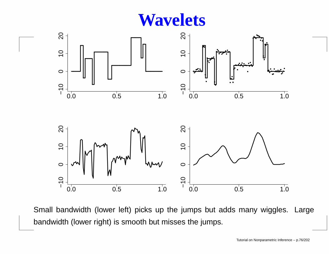
Small bandwidth (lower left) picks up the jumps but adds many wiggles. Large
bandwidth (lower right) is smooth but misses the jumps.
Tutorial on Nonparametric Inference – p.76/202
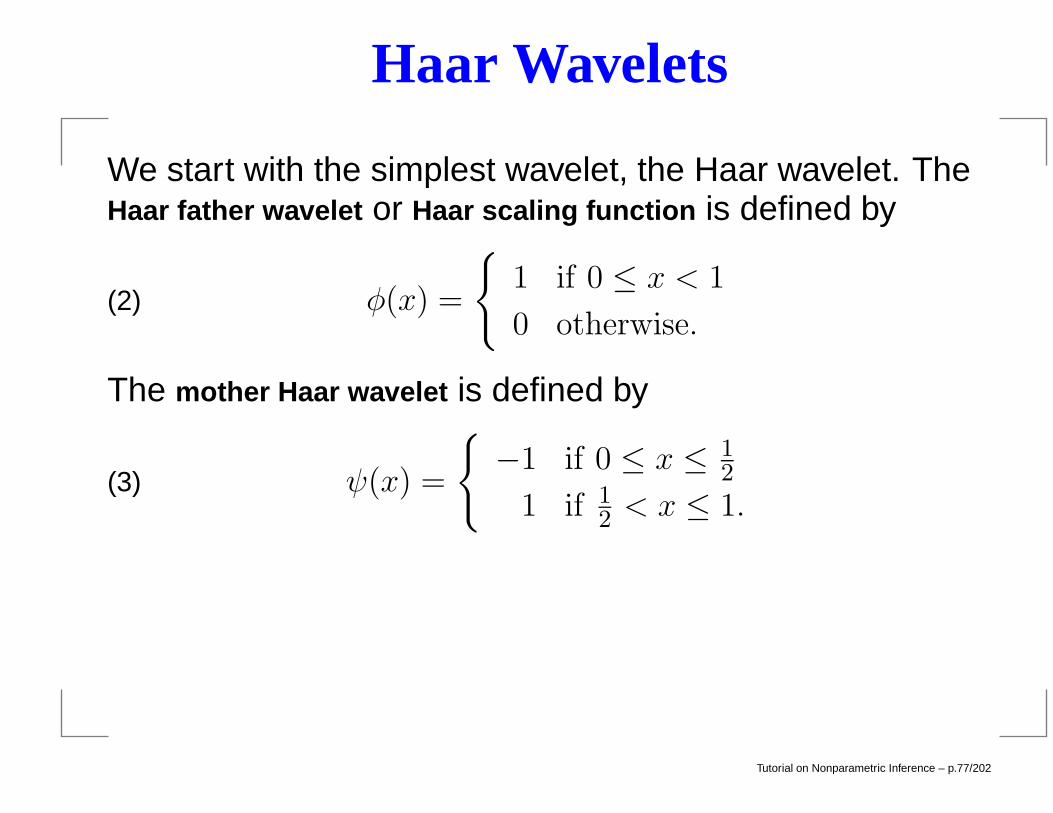
Haar Wavelets
We start with the simplest wavelet, the Haar wavelet. TheHaar father wavelet or Haar scaling function is defined by
φ(x) =
1 if 0 ≤ x < 1
0 otherwise.(2)
The mother Haar wavelet is defined by
ψ(x) =
−1 if 0 ≤ x ≤ 1
2
1 if 12 < x ≤ 1.
(3)
Tutorial on Nonparametric Inference – p.77/202
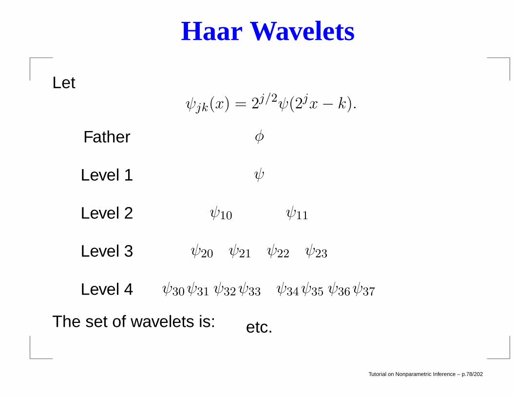
Haar Wavelets
Letψjk(x) = 2j/2ψ(2jx− k).
The set of wavelets is:
φ
ψ
ψ10 ψ11
ψ20 ψ21 ψ22 ψ23
ψ30ψ31 ψ32ψ33 ψ34ψ35 ψ36ψ37
Father
Level 1
Level 2
Level 3
Level 4
etc.
Tutorial on Nonparametric Inference – p.78/202
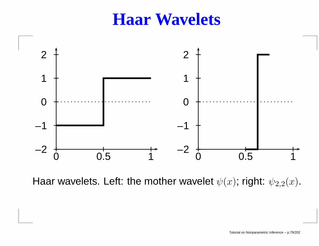
Haar Wavelets
–2
–1
0
1
2
0 0.5 1–2
–1
0
1
2
0 0.5 1Some
Haar wavelets. Left: the mother wavelet ψ(x); right: ψ2,2(x).
Tutorial on Nonparametric Inference – p.79/202
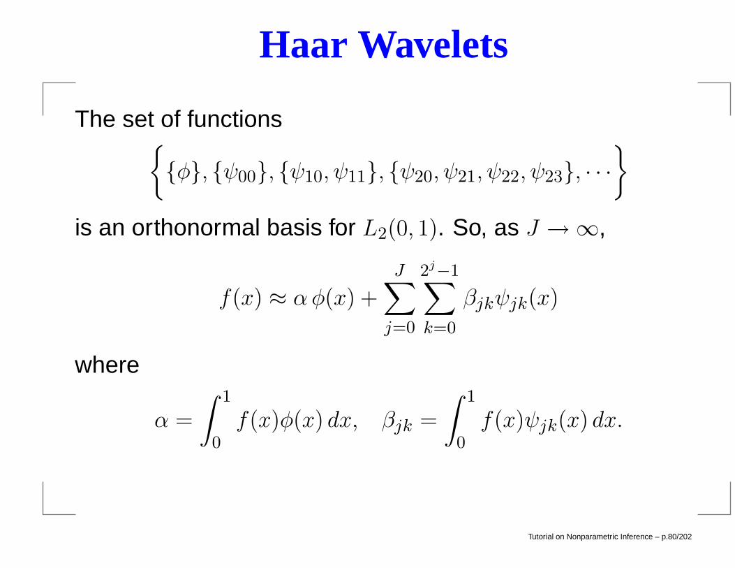
Haar Wavelets
The set of functionsφ, ψ00, ψ10, ψ11, ψ20, ψ21, ψ22, ψ23, · · ·
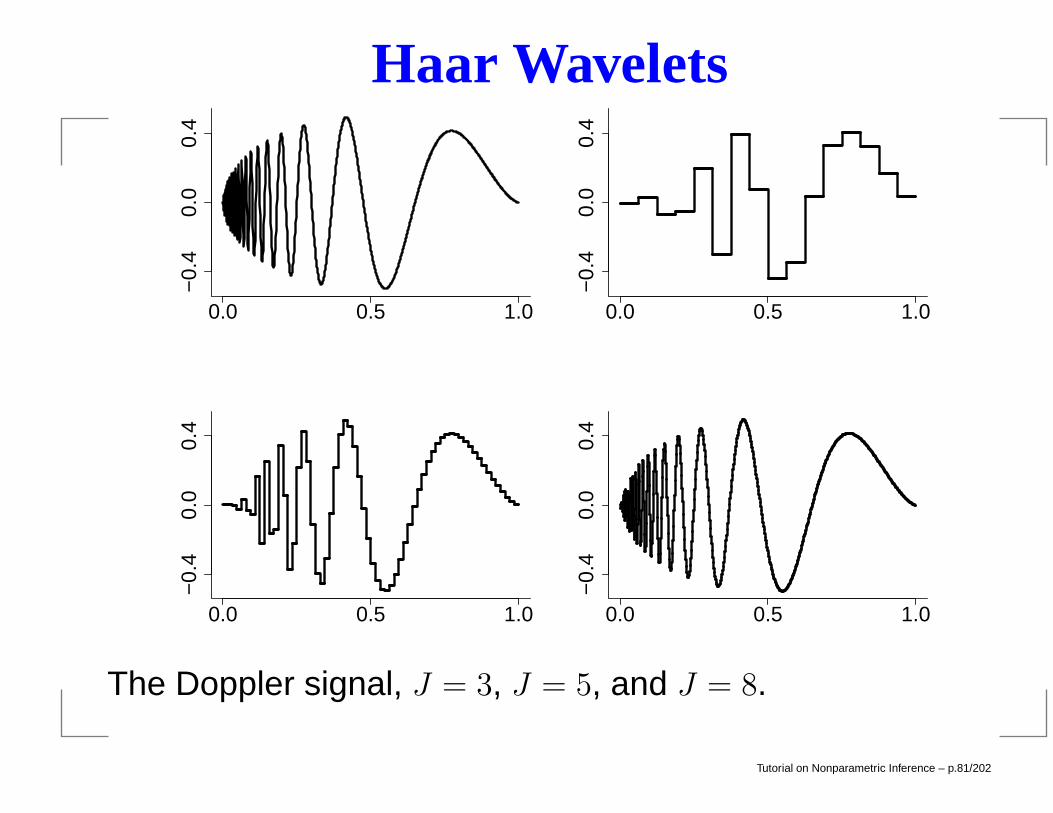
is an orthonormal basis for L2(0, 1). So, as J →∞,
f(x) ≈ αφ(x) +
J∑
j=0
2j−1∑
k=0
βjkψjk(x)
where
α =
∫ 1
0f(x)φ(x) dx, βjk =
∫ 1
0f(x)ψjk(x) dx.
Tutorial on Nonparametric Inference – p.80/202
Haar Wavelets
0.0 0.5 1.0
−0.
40.
00.
4
0.0 0.5 1.0
−0.
40.
00.
40.0 0.5 1.0
−0.
40.
00.
4
0.0 0.5 1.0−
0.4
0.0
0.4
The Doppler signal, J = 3, J = 5, and J = 8.
Tutorial on Nonparametric Inference – p.81/202
Haar Wavelets
0.0 0.5 1.0
Tutorial on Nonparametric Inference – p.82/202
Haar Wavelets
Many functions f have sparse expansions in a wavelet basis.Smooth functions are sparse. (Smooth + jumps) is alsosparse. So, we expect that for many functions we can write
f(x) = αφ(x) +∑
j
∑
j
βjkψjk(x)
where most βjk ≈ 0.The idea is to estimate the β′jks then set all βjk = 0 exceptfor a few large coefficients.
Tutorial on Nonparametric Inference – p.83/202
Smoother Wavelets
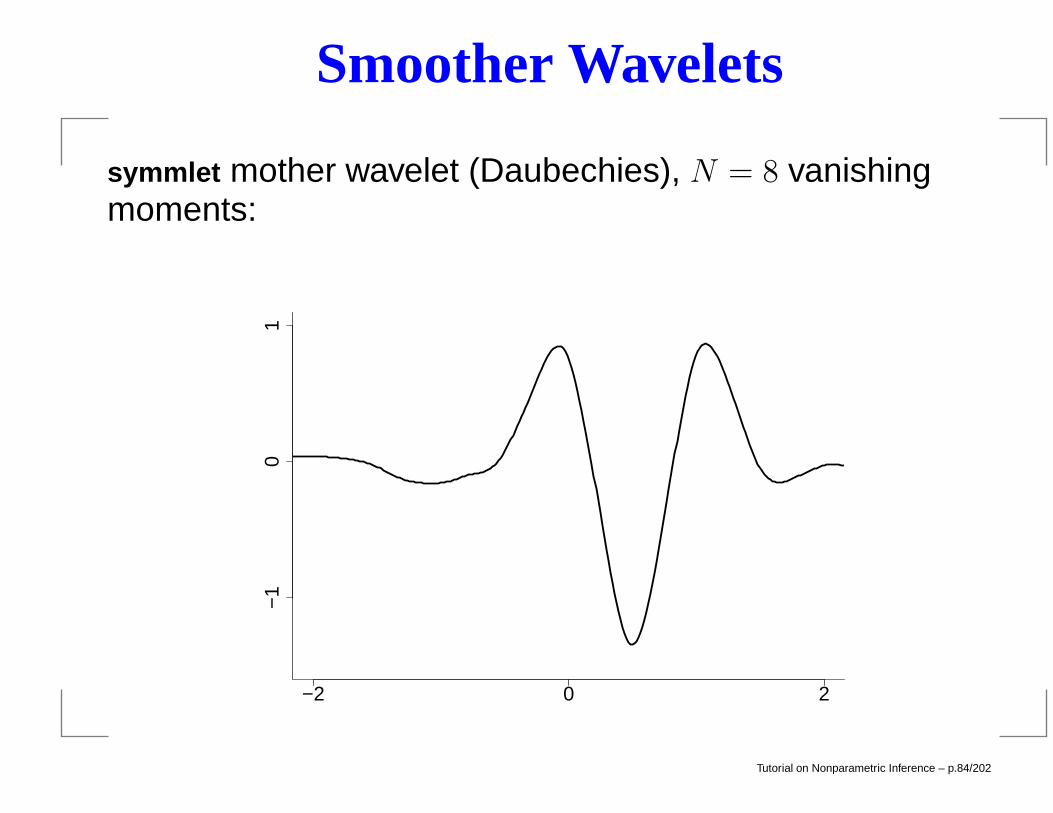
symmlet mother wavelet (Daubechies), N = 8 vanishingmoments:
−2 0 2
−1
01
Tutorial on Nonparametric Inference – p.84/202
Smoother Wavelets
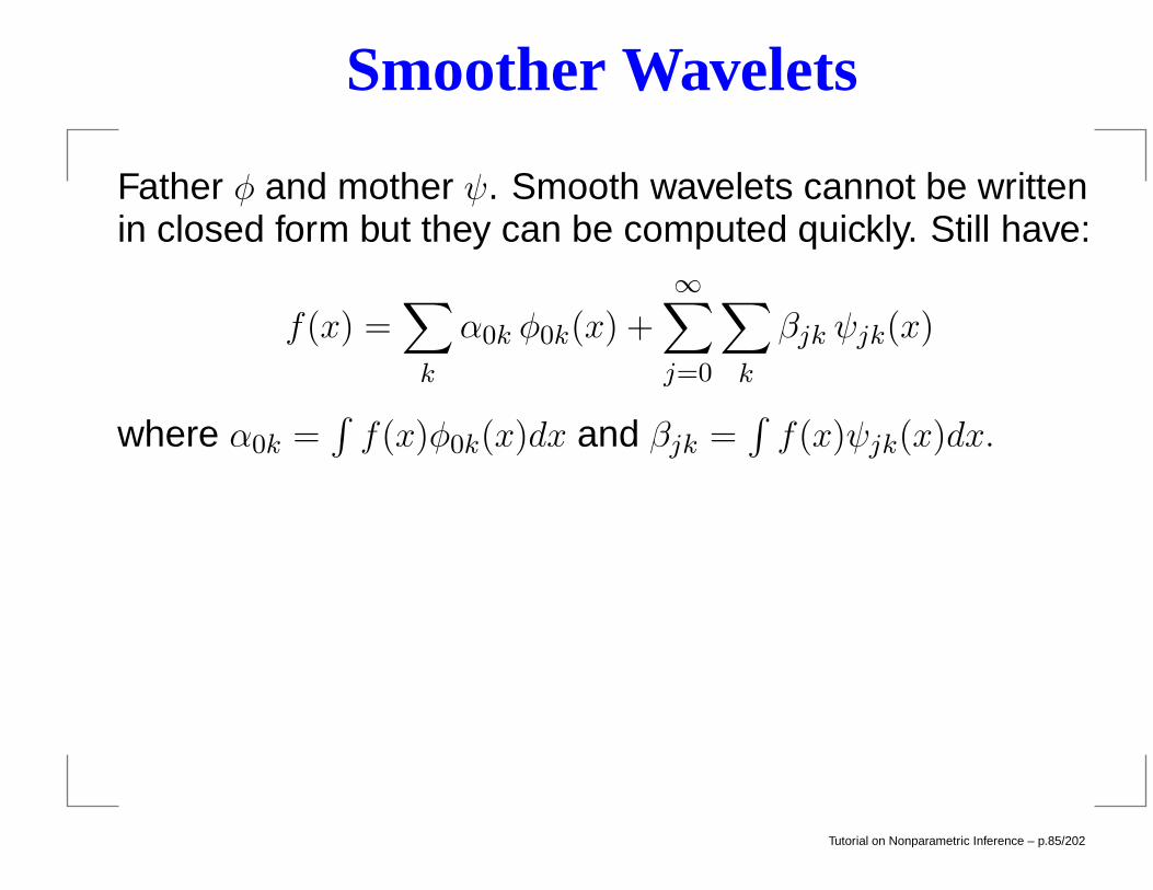
Father φ and mother ψ. Smooth wavelets cannot be writtenin closed form but they can be computed quickly. Still have:
f(x) =∑
k
α0k φ0k(x) +
∞∑
j=0
∑
k
βjk ψjk(x)
where α0k =∫f(x)φ0k(x)dx and βjk =
∫f(x)ψjk(x)dx.
Tutorial on Nonparametric Inference – p.85/202
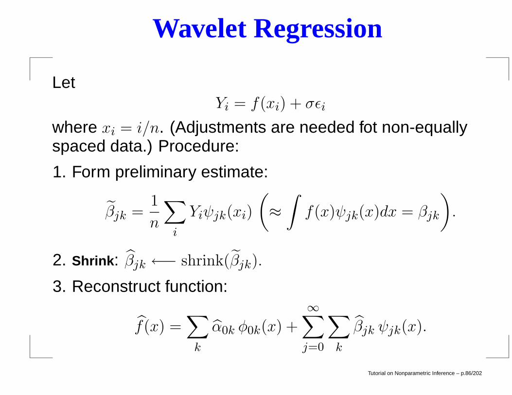
Wavelet Regression
LetYi = f(xi) + σεi
where xi = i/n. (Adjustments are needed fot non-equallyspaced data.) Procedure:
1. Form preliminary estimate:
βjk =1
n
∑
i
Yiψjk(xi)
(≈∫f(x)ψjk(x)dx = βjk
).
2. Shrink: βjk ←− shrink(βjk).
3. Reconstruct function:
f(x) =∑
k
α0k φ0k(x) +
∞∑
j=0
∑
k
βjk ψjk(x).
Tutorial on Nonparametric Inference – p.86/202
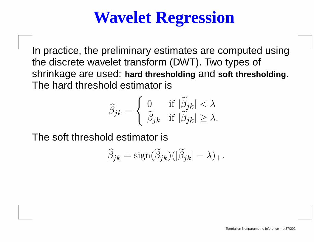
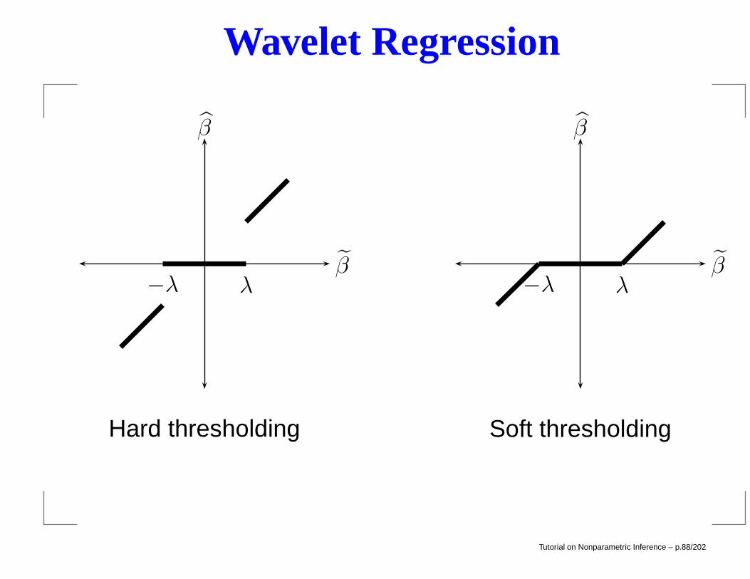
Wavelet Regression
In practice, the preliminary estimates are computed usingthe discrete wavelet transform (DWT). Two types ofshrinkage are used: hard thresholding and soft thresholding.The hard threshold estimator is
βjk =
0 if |βjk| < λ
βjk if |βjk| ≥ λ.
The soft threshold estimator is
βjk = sign(βjk)(|βjk| − λ)+.
Tutorial on Nonparametric Inference – p.87/202
Wavelet Regression
λ−λβ
β
Hard thresholding
λ−λβ
β
Soft thresholding
Tutorial on Nonparametric Inference – p.88/202
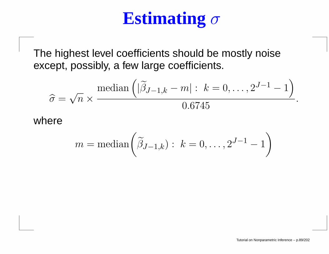
Estimating σ
The highest level coefficients should be mostly noiseexcept, possibly, a few large coefficients.
σ =√n×
median(|βJ−1,k −m| : k = 0, . . . , 2J−1 − 1
)
0.6745.
where
m = median
(βJ−1,k) : k = 0, . . . , 2J−1 − 1
)
Tutorial on Nonparametric Inference – p.89/202
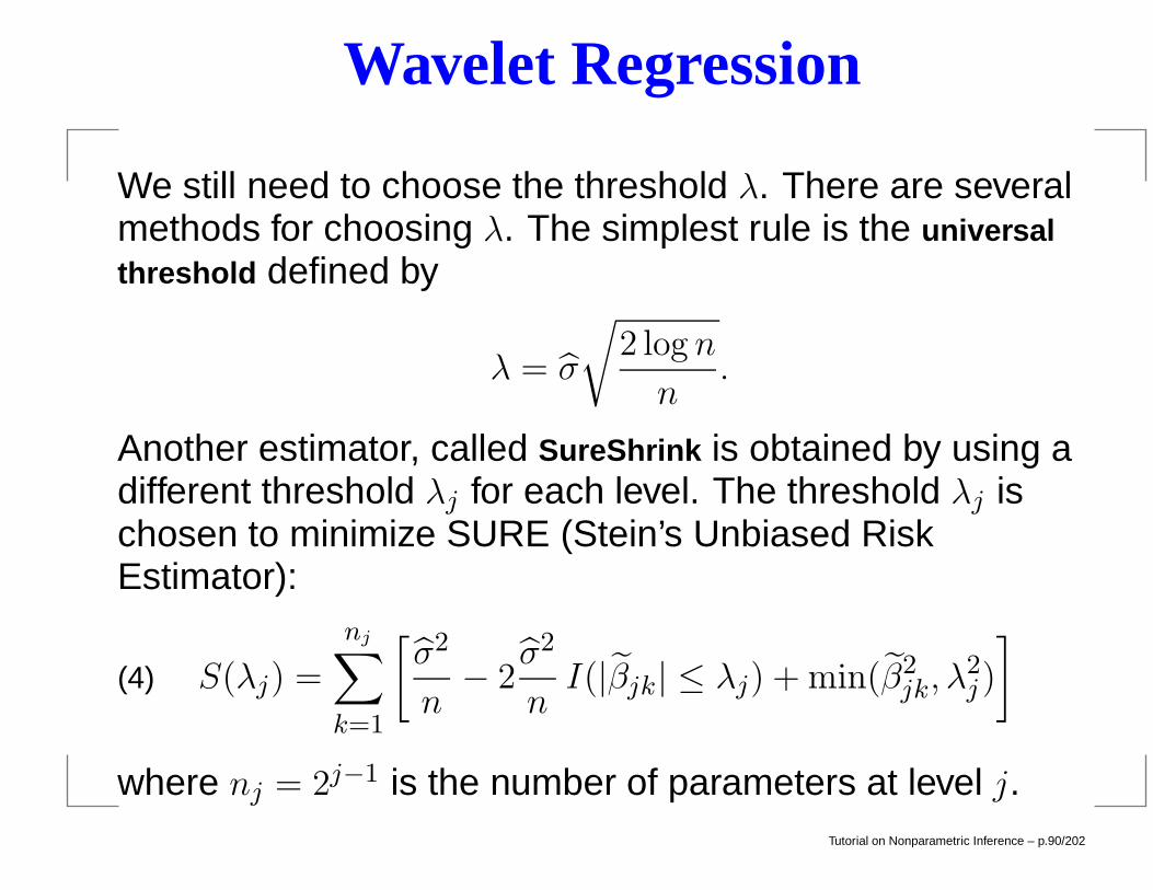
Wavelet Regression
We still need to choose the threshold λ. There are severalmethods for choosing λ. The simplest rule is the universalthreshold defined by
λ = σ
√2 log n
n.
Another estimator, called SureShrink is obtained by using adifferent threshold λj for each level. The threshold λj ischosen to minimize SURE (Stein’s Unbiased RiskEstimator):
S(λj) =
nj∑
k=1
[σ2
n− 2
σ2
nI(|βjk| ≤ λj) + min(β2
jk, λ2j )
](4)
where nj = 2j−1 is the number of parameters at level j.Tutorial on Nonparametric Inference – p.90/202
Example
0.0 0.5 1.0
−10
0
10
20
0.0 0.5 1.0
−10
0
10
20
0.0 0.5 1.0
−10
0
20
0.0 0.5 1.0
−10
0
20
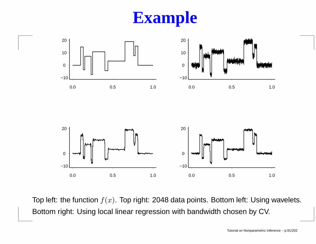
Top left: the function f(x). Top right: 2048 data points. Bottom left: Using wavelets.
Bottom right: Using local linear regression with bandwidth chosen by CV.
Tutorial on Nonparametric Inference – p.91/202
Wavelet Regression in R
Include library wavethresh.
Assumes y has length which is power of two: Interpolate asneeded:> library(wavethresh)
> xs = seq(1,700,length=512)
> lo = floor(xs)
> hi = ceiling(xs)
> ys = (xs-lo)*wmap$Cl[hi] + (hi-xs)*wmap$Cl[lo] +
wmap$Cl[lo]*(lo==hi)
Tutorial on Nonparametric Inference – p.92/202
Wavelet Regression in R
The function wd() does the initial wavelet transform:
> waveletwmap = wd(ys, family="DaubLeAsymm", filter.number=8)
Argument family="DaubLeAsymm" gives the Daubechiessymmlet
Argument filter.number=8 sets N = 8 (eight vanishingmoments)
Tutorial on Nonparametric Inference – p.93/202
Wavelet Regression in R
The function threshold() does soft and hardthresholding:> softthreshwmap = threshold(waveletwmap,type="soft",
policy="universal")
> hardthreshwmap = threshold(waveletwmap,type="hard",
policy="universal")
Argument policy="universal" specifies universalthresholding
To invert the transform (i.e., get fitted values) usewr(softthreshwmap)
Tutorial on Nonparametric Inference – p.94/202
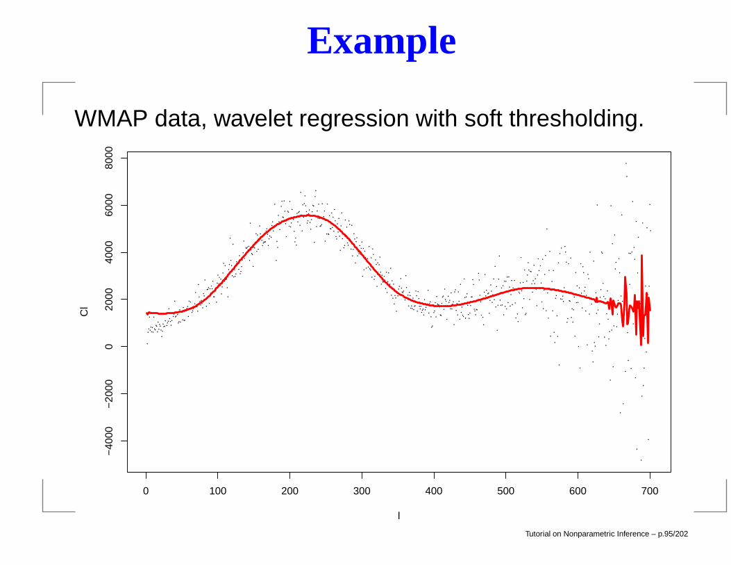
Example
WMAP data, wavelet regression with soft thresholding.
0 100 200 300 400 500 600 700
−40
00−
2000
020
0040
0060
0080
00
l
Cl
Tutorial on Nonparametric Inference – p.95/202
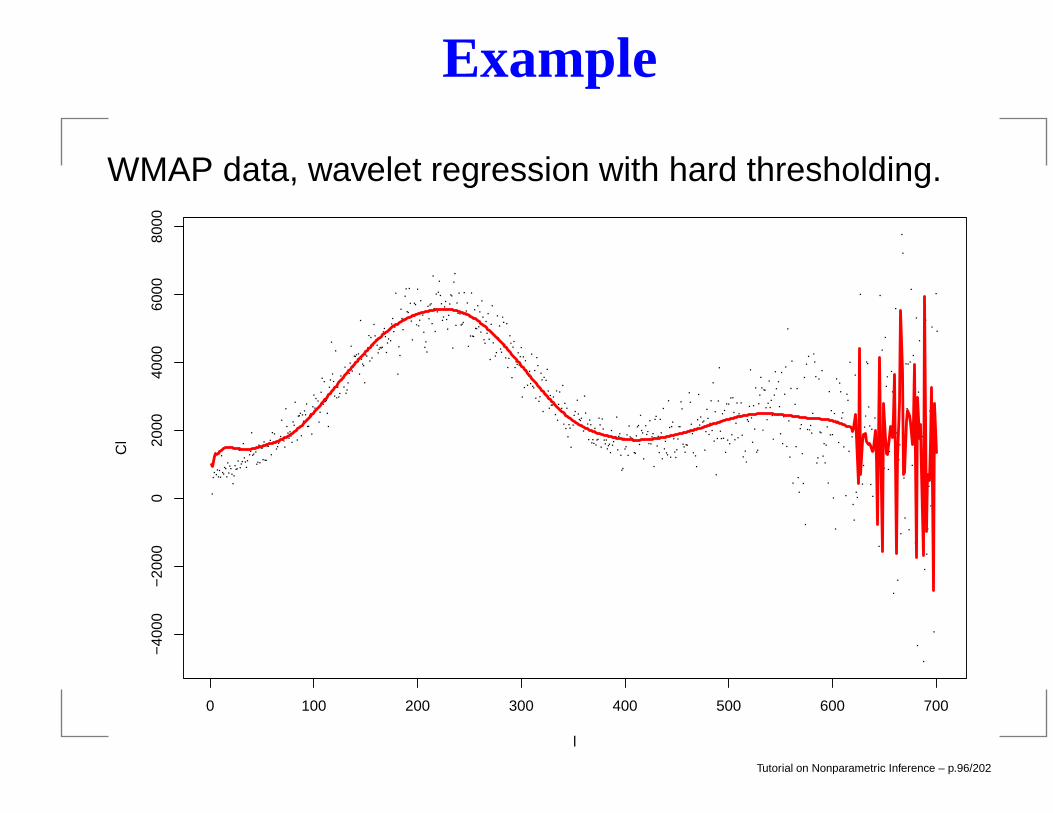
Example
WMAP data, wavelet regression with hard thresholding.
0 100 200 300 400 500 600 700
−40
00−
2000
020
0040
0060
0080
00
l
Cl
Tutorial on Nonparametric Inference – p.96/202
Multiple Regression
Y = f(X1, X2, . . . , Xd) + ε
The curse of dimensionality:Optimal rate of convergence for d = 1 is n−4/5. In ddimensions the optimal rate of convergence is is n−4/(4+d).Thus, the sample size m required for a d-dimensionalproblem to have the same accuracy as a sample size n in aone-dimensional problem is m ∝ ncd wherec = (4 + d)/(5d) > 0.
To maintain a given degree of accuracy of an estimator, thesample size must increase exponentially with the dimension d.
Put another way, confidence bands get very large as the di-mension d increases.
Tutorial on Nonparametric Inference – p.97/202
Multiple Local Linear
Given a nonsingular positive definite d× d bandwidth matrixH, we define
KH(x) =1
|H|1/2K(H−1/2x).
Often, one scales each covariate to have the same meanand variance and then we use the kernel
h−dK(||x||/h)where K is any one-dimensional kernel. Then there is asingle bandwidth parameter h.
Tutorial on Nonparametric Inference – p.98/202
Multiple Local Linear
At a target value x = (x1, . . . , xd)T , the local sum of squares
is given by
n∑
i=1
wi(x)
(Yi − a0 −
d∑
j=1
aj(xij − xj))2
wherewi(x) = K(||xi − x||/h).
The estimator is fn(x) = a0 a = (a0, . . . , ad)T is the value
of a = (a0, . . . , ad)T that minimizes the weighted sums of
squares.
Tutorial on Nonparametric Inference – p.99/202
Multiple Local Linear
The solution a is
a = (XTxWxXx)
−1XTxWxY
where
Xx =
1 (x11 − x1) · · · (x1d − xd)1 (x21 − x1) · · · (x2d − xd)...
... . . . ...1 (xn1 − x1) · · · (xnd − xd)
and Wx is the diagonal matrix whose (i, i) element is wi(x).
Tutorial on Nonparametric Inference – p.100/202
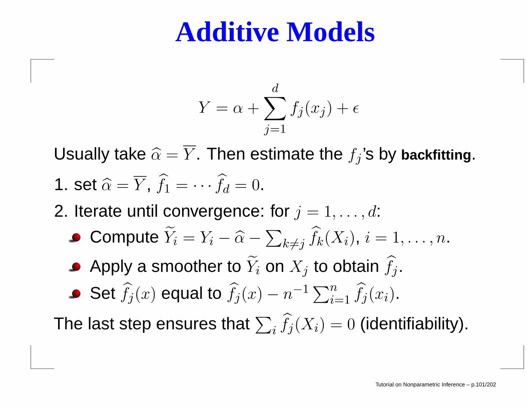
Additive Models
Y = α+d∑
j=1
fj(xj) + ε
Usually take α = Y . Then estimate the fj ’s by backfitting.
1. set α = Y , f1 = · · · fd = 0.
2. Iterate until convergence: for j = 1, . . . , d:
Compute Yi = Yi − α−∑
k 6=j fk(Xi), i = 1, . . . , n.
Apply a smoother to Yi on Xj to obtain fj.
Set fj(x) equal to fj(x)− n−1∑n
i=1 fj(xi).
The last step ensures that∑
i fj(Xi) = 0 (identifiability).
Tutorial on Nonparametric Inference – p.101/202
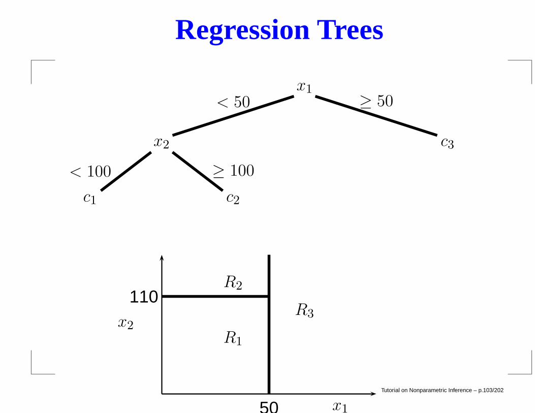
Regression Trees
A regression tree is a model of the form
f(x) =
M∑
m=1
Y mI(x ∈ Rm)
where R1, . . . , RM are disjoint rectangles.
Tutorial on Nonparametric Inference – p.102/202
Regression Trees
c1 c2
x2 c3
x1
< 100 ≥ 100
< 50 ≥ 50
R3
R1
R2
x1
x2
50
110
Tutorial on Nonparametric Inference – p.103/202

Regression Trees
Generally one grows a very large tree, then the tree ispruned to form a subtree by collapsing regions together.The size of the tree is a tuning parameter chosen asfollows. Let Nm denote the number of points in a rectangleRm of a subtree T and define
cm =1
Nm
∑
xi∈Rm
Yi, Qm(T ) =1
Nm
∑
xi∈Rm
(Yi − cm)2.
Tutorial on Nonparametric Inference – p.104/202
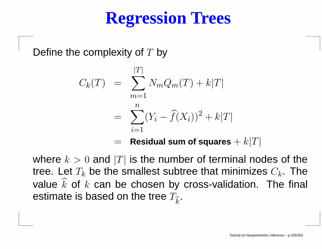
Regression Trees
Define the complexity of T by
Ck(T ) =
|T |∑
m=1
NmQm(T ) + k|T |
=
n∑
i=1
(Yi − f(Xi))2 + k|T |
= Residual sum of squares + k|T |where k > 0 and |T | is the number of terminal nodes of thetree. Let Tk be the smallest subtree that minimizes Ck. Thevalue k of k can be chosen by cross-validation. The finalestimate is based on the tree T
k.
Tutorial on Nonparametric Inference – p.105/202
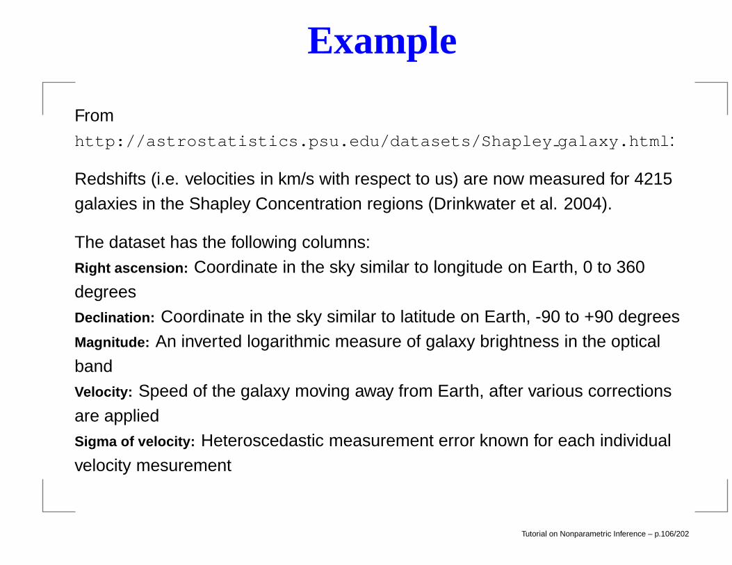
Example
Fromhttp://astrostatistics.psu.edu/datasets/Shapley galaxy.html:
Redshifts (i.e. velocities in km/s with respect to us) are now measured for 4215
galaxies in the Shapley Concentration regions (Drinkwater et al. 2004).
The dataset has the following columns:
Right ascension: Coordinate in the sky similar to longitude on Earth, 0 to 360degrees
Declination: Coordinate in the sky similar to latitude on Earth, -90 to +90 degreesMagnitude: An inverted logarithmic measure of galaxy brightness in the optical
bandVelocity: Speed of the galaxy moving away from Earth, after various corrections
are appliedSigma of velocity: Heteroscedastic measurement error known for each individual
velocity mesurement
Tutorial on Nonparametric Inference – p.106/202
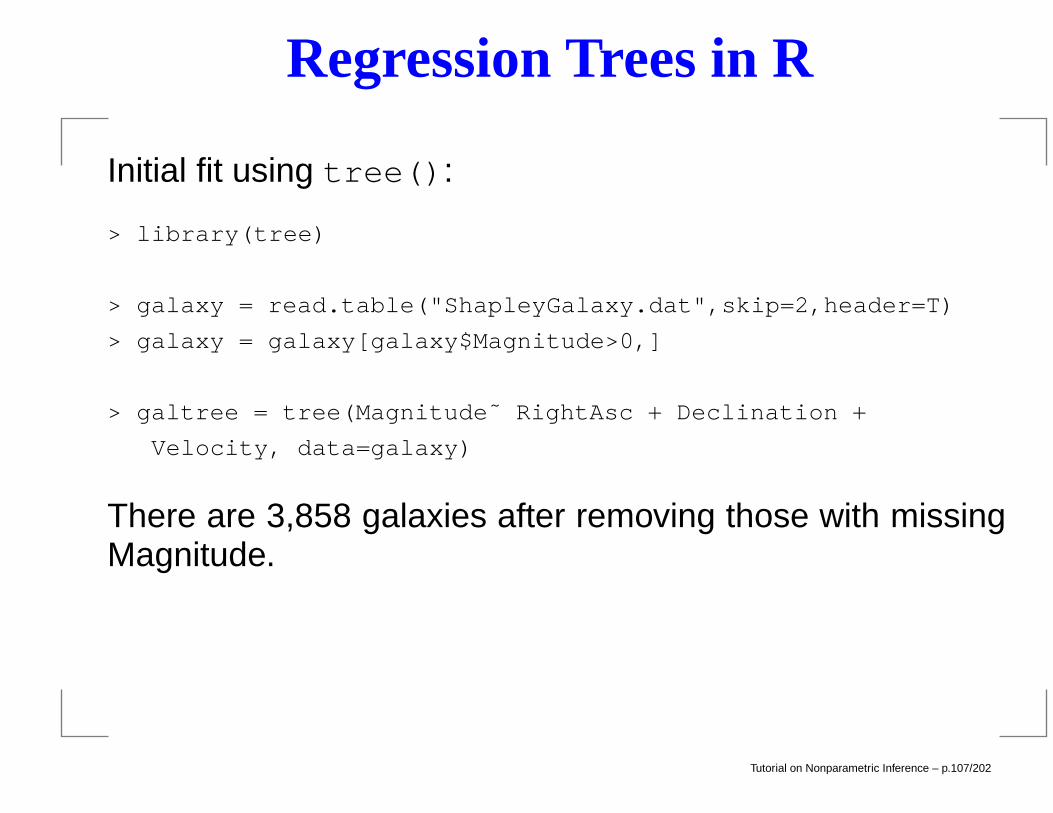
Regression Trees in R
Initial fit using tree():
> library(tree)
> galaxy = read.table("ShapleyGalaxy.dat",skip=2,header=T)
> galaxy = galaxy[galaxy$Magnitude>0,]
> galtree = tree(Magnitude˜ RightAsc + Declination +
Velocity, data=galaxy)
There are 3,858 galaxies after removing those with missingMagnitude.
Tutorial on Nonparametric Inference – p.107/202
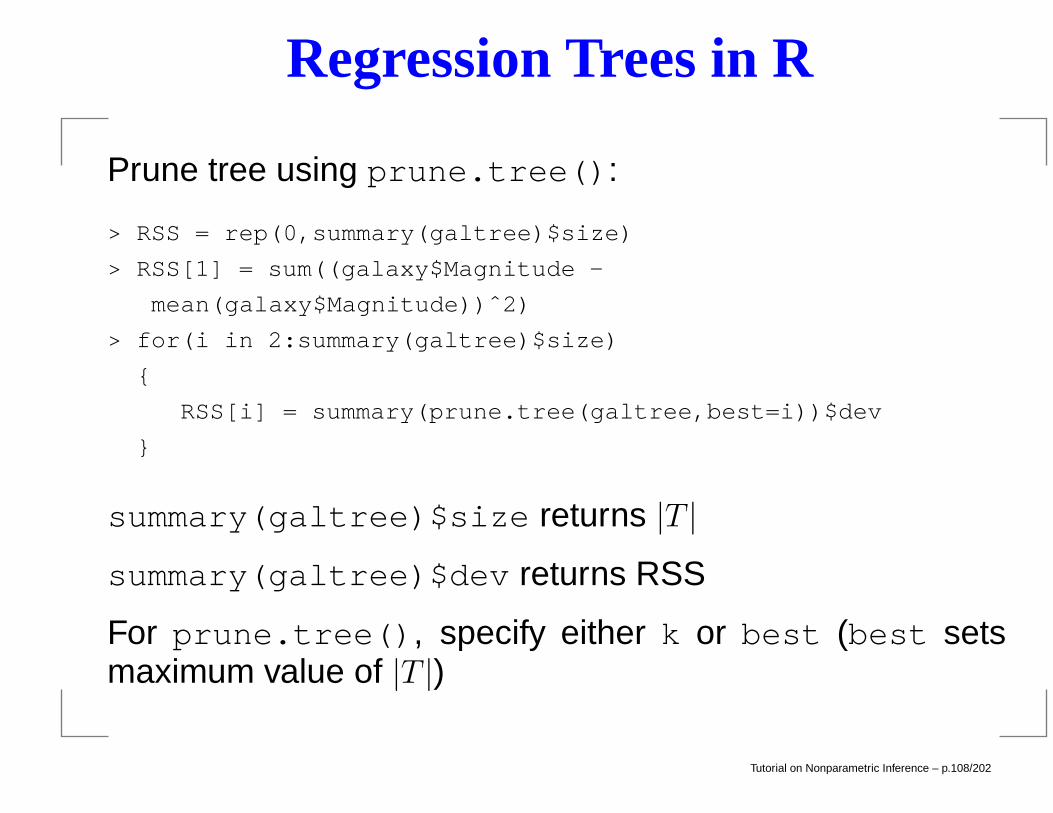
Regression Trees in R
Prune tree using prune.tree():
> RSS = rep(0,summary(galtree)$size)
> RSS[1] = sum((galaxy$Magnitude -
mean(galaxy$Magnitude))ˆ2)
> for(i in 2:summary(galtree)$size)
RSS[i] = summary(prune.tree(galtree,best=i))$dev
summary(galtree)$size returns |T |summary(galtree)$dev returns RSS
For prune.tree(), specify either k or best (best setsmaximum value of |T |)
Tutorial on Nonparametric Inference – p.108/202
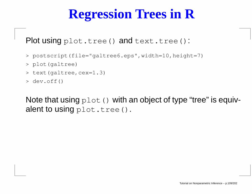
Regression Trees in R
Plot using plot.tree() and text.tree():
> postscript(file="galtree6.eps",width=10,height=7)
> plot(galtree)
> text(galtree,cex=1.3)
> dev.off()
Note that using plot() with an object of type “tree” is equiv-alent to using plot.tree().
Tutorial on Nonparametric Inference – p.109/202
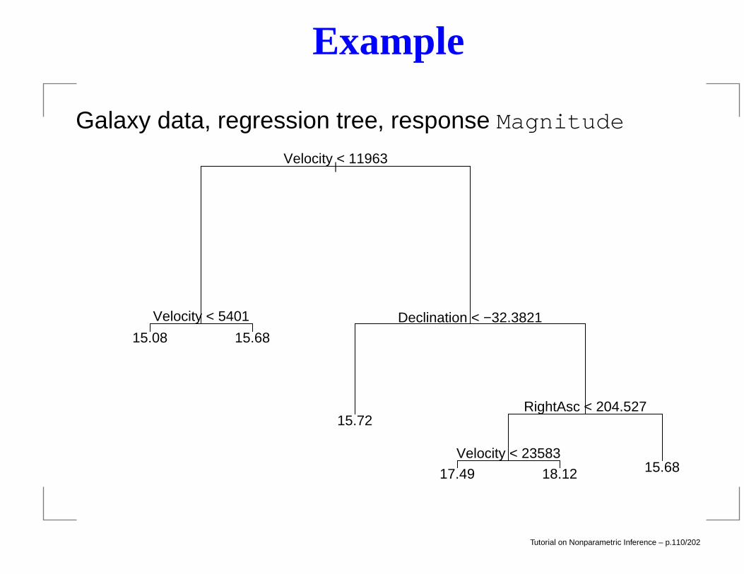
Example
Galaxy data, regression tree, response Magnitude
|Velocity < 11963
Velocity < 5401 Declination < −32.3821
RightAsc < 204.527
Velocity < 23583
15.08 15.68
15.72
17.49 18.12 15.68
Tutorial on Nonparametric Inference – p.110/202
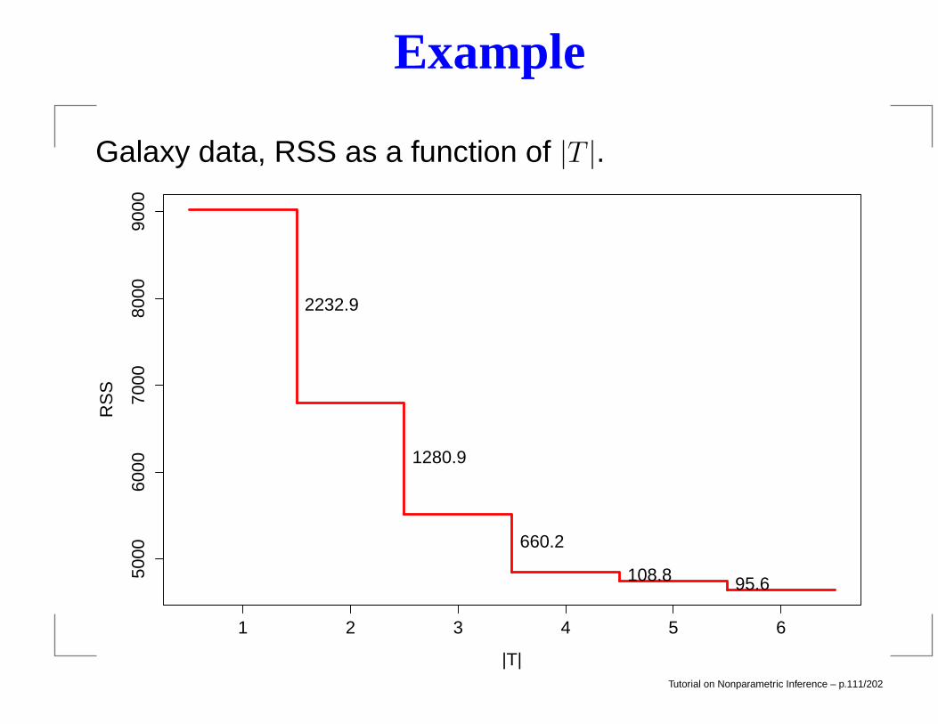
Example
Galaxy data, RSS as a function of |T |.
1 2 3 4 5 6
5000
6000
7000
8000
9000
|T|
RS
S
2232.9
1280.9
660.2
108.8 95.6
Tutorial on Nonparametric Inference – p.111/202
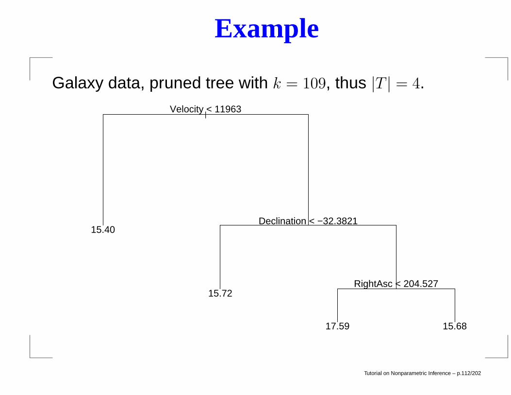
Example
Galaxy data, pruned tree with k = 109, thus |T | = 4.
|Velocity < 11963
Declination < −32.3821
RightAsc < 204.527
15.40
15.72
17.59 15.68
Tutorial on Nonparametric Inference – p.112/202
Density Estimation
ObserveX1, . . . , Xn ∼ f.
Want to estimate f . Methods include:
1. binning (histogram)
2. kernel estimator
3. local likelihood
4. wavelets
Tutorial on Nonparametric Inference – p.113/202
Density Estimation
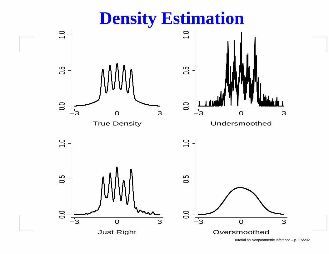
Example: Bart Simpson.
f(x) =1
2φ(x; 0, 1) +
1
10
4∑
j=0
φ(x; (j/2)− 1, 1/10)
where φ(x;µ, σ) denotes a Normal density with mean µ andstandard deviation σ. This is a nasty density.
Tutorial on Nonparametric Inference – p.114/202
Density Estimation
−3 0 3
0.00.5
1.0
True Density
−3 0 3
0.00.5
1.0
Undersmoothed
−3 0 3
0.00.5
1.0
Just Right
−3 0 3
0.00.5
1.0
OversmoothedTutorial on Nonparametric Inference – p.115/202
histogram
Create bins B1, B2, . . . , Bm of width h. Define
fn(x) =m∑
j=1
pjhI(x ∈ Bj).
where pj is proportion of observations in Bj. Note that∫fn(x)dx = 1.
Tutorial on Nonparametric Inference – p.116/202
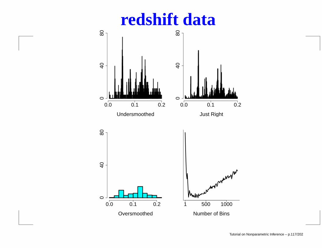
redshift data
0.0 0.1 0.20
4080
Undersmoothed
0.0 0.1 0.2
040
80
Just Right
0.0 0.1 0.2
040
80
Oversmoothed
1 500 1000
Number of Bins
Tutorial on Nonparametric Inference – p.117/202
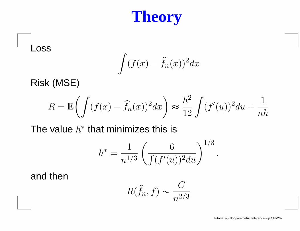
Theory
Loss ∫(f(x)− fn(x))2dx
Risk (MSE)
R = E
(∫(f(x)− fn(x))2dx
)≈ h2
12
∫(f ′(u))2du+
1
nh
The value h∗ that minimizes this is
h∗ =1
n1/3
(6∫
(f ′(u))2du
)1/3
.
and then
R(fn, f) ∼ C
n2/3
Tutorial on Nonparametric Inference – p.118/202
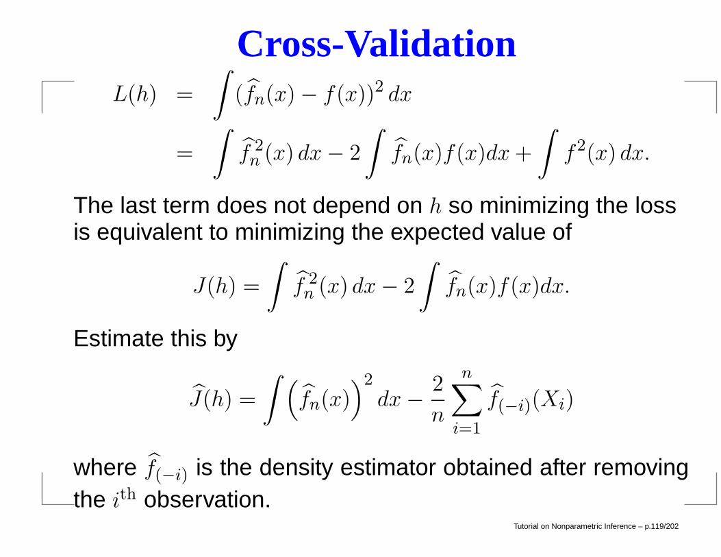
Cross-ValidationL(h) =
∫(fn(x)− f(x))2 dx
=
∫f 2n (x) dx− 2
∫fn(x)f(x)dx+
∫f2(x) dx.
The last term does not depend on h so minimizing the lossis equivalent to minimizing the expected value of
J(h) =
∫f 2n (x) dx− 2
∫fn(x)f(x)dx.
Estimate this by
J(h) =
∫ (fn(x)
)2
dx− 2
n
n∑
i=1
f(−i)(Xi)
where f(−i) is the density estimator obtained after removingthe ith observation.
Tutorial on Nonparametric Inference – p.119/202
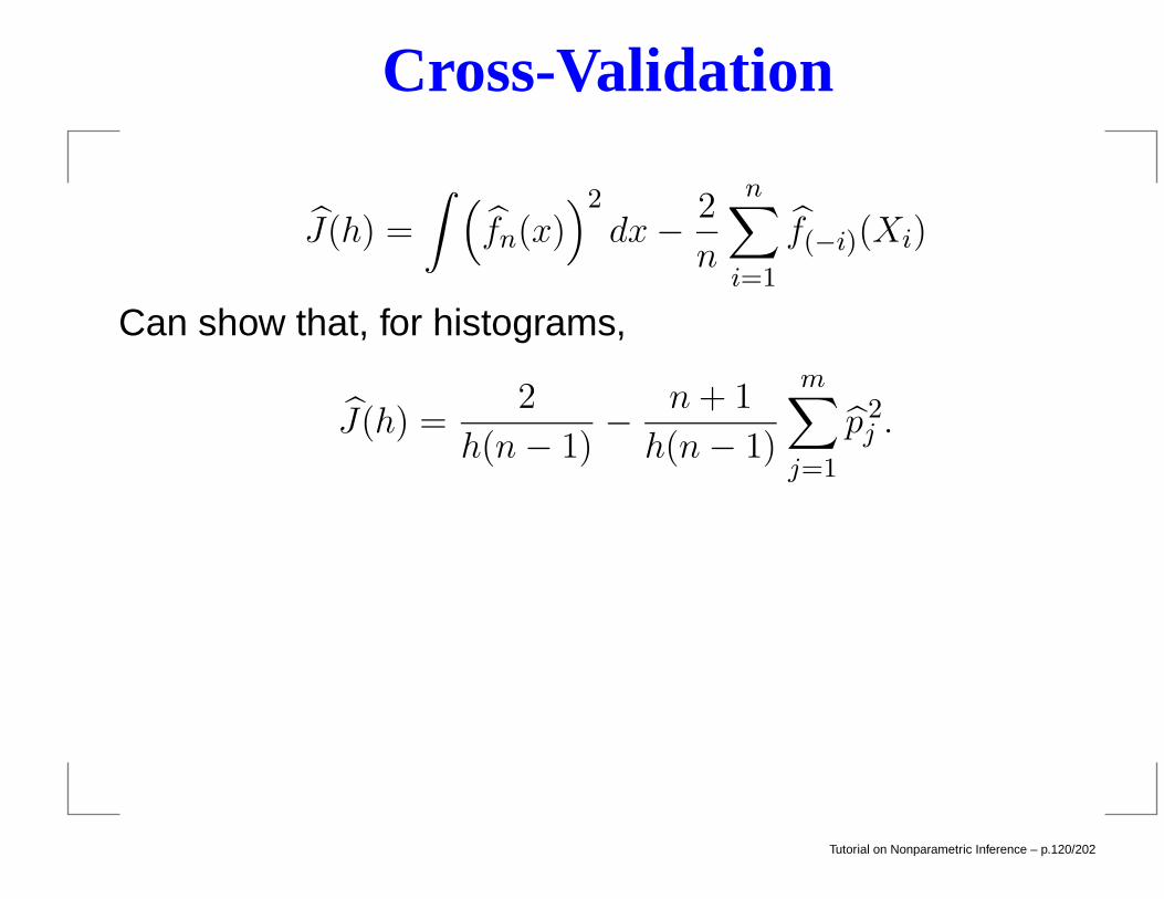
Cross-Validation
J(h) =
∫ (fn(x)
)2
dx− 2
n
n∑
i=1
f(−i)(Xi)
Can show that, for histograms,
J(h) =2
h(n− 1)− n+ 1
h(n− 1)
m∑
j=1
p 2j .
Tutorial on Nonparametric Inference – p.120/202
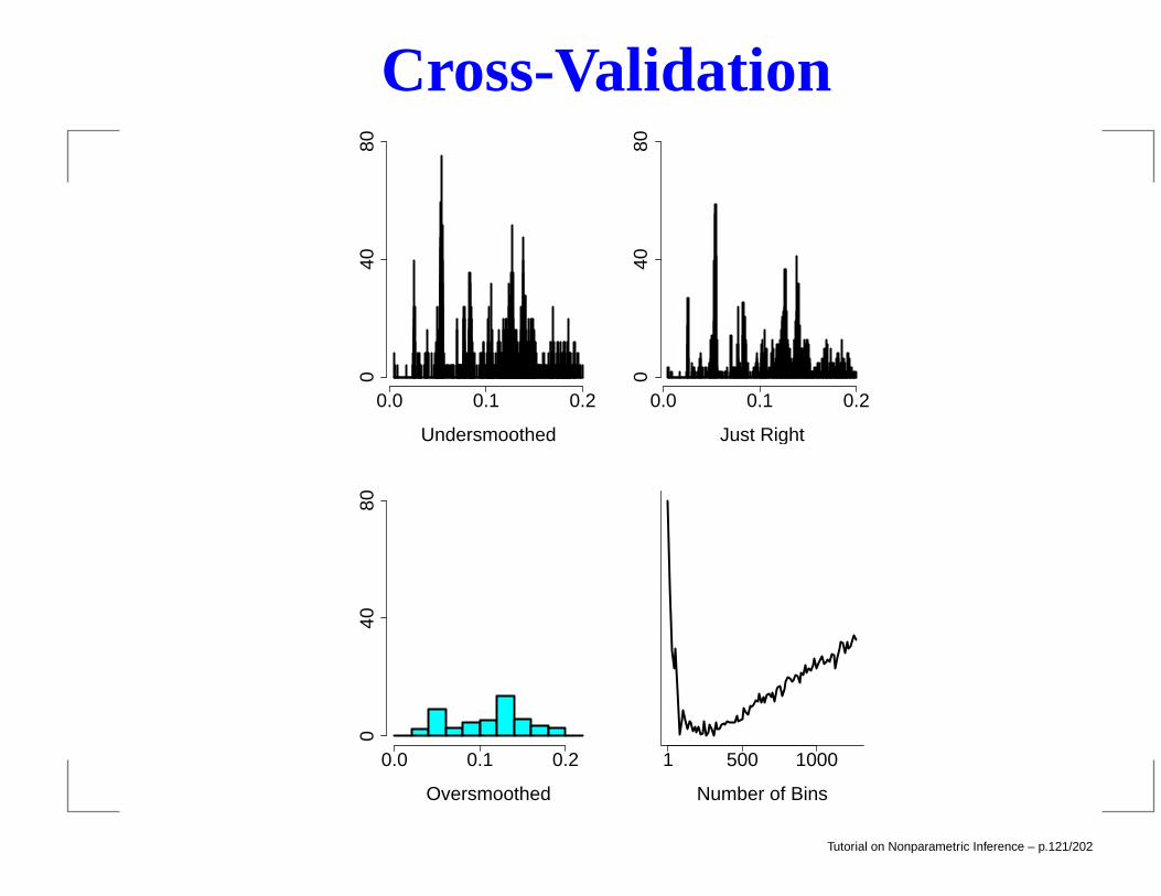
Cross-Validation
0.0 0.1 0.2
040
80
Undersmoothed
0.0 0.1 0.2
040
80
Just Right
0.0 0.1 0.2
040
80
Oversmoothed
1 500 1000
Number of Bins
Tutorial on Nonparametric Inference – p.121/202
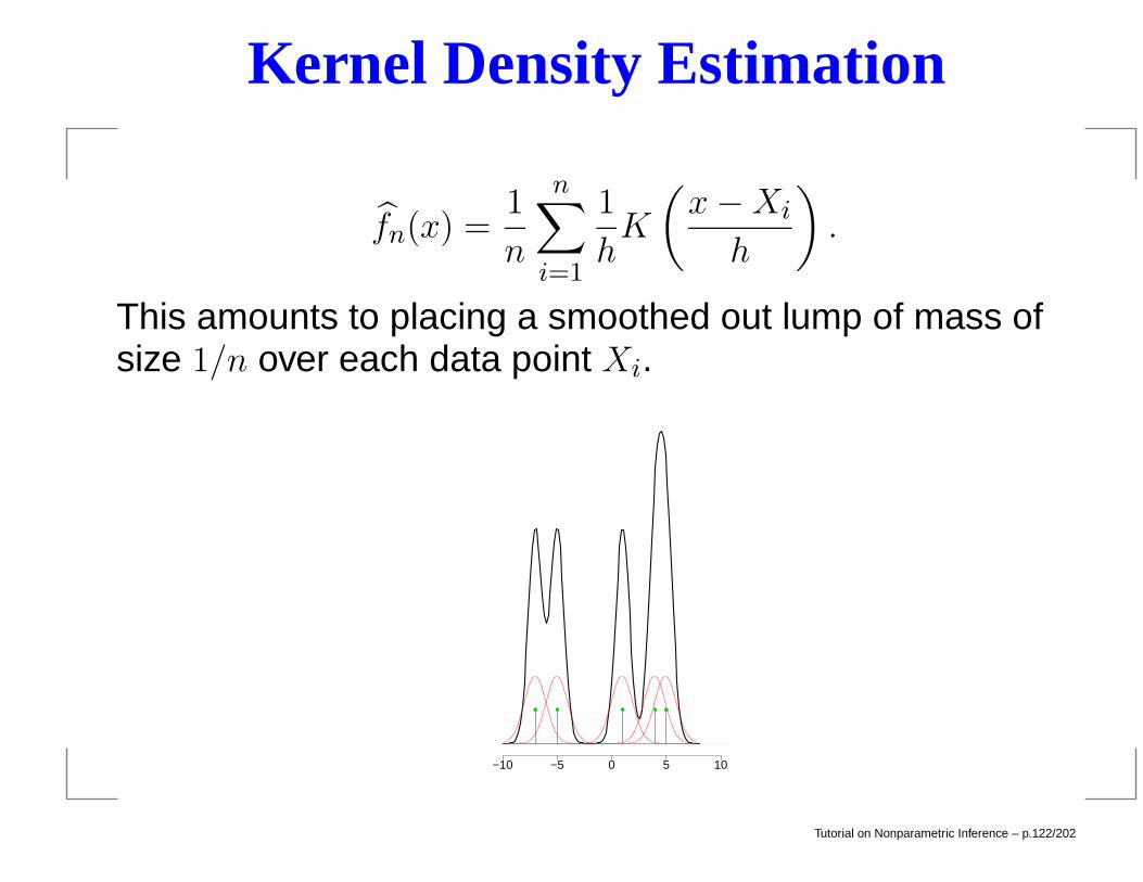
Kernel Density Estimation
fn(x) =1
n
n∑
i=1
1
hK
(x−Xi
h
).
This amounts to placing a smoothed out lump of mass ofsize 1/n over each data point Xi.
−10 −5 0 5 10
Tutorial on Nonparametric Inference – p.122/202
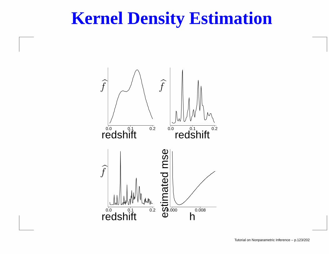
Kernel Density Estimation
0.0 0.1 0.2 0.0 0.1 0.2
0.0 0.1 0.2 0.000 0.008
f f
fes
timat
edm
se
redshift redshift
redshift h
Tutorial on Nonparametric Inference – p.123/202
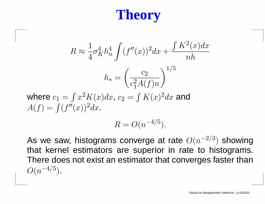
Theory
R ≈ 1
4σ4Kh
4n
∫(f ′′(x))2dx+
∫K2(x)dx
nh
h∗ =
(c2
c21A(f)n
)1/5
where c1 =∫x2K(x)dx, c2 =
∫K(x)2dx and
A(f) =∫
(f ′′(x))2dx.
R = O(n−4/5).
As we saw, histograms converge at rate O(n−2/3) showingthat kernel estimators are superior in rate to histograms.There does not exist an estimator that converges faster thanO(n−4/5).
Tutorial on Nonparametric Inference – p.124/202
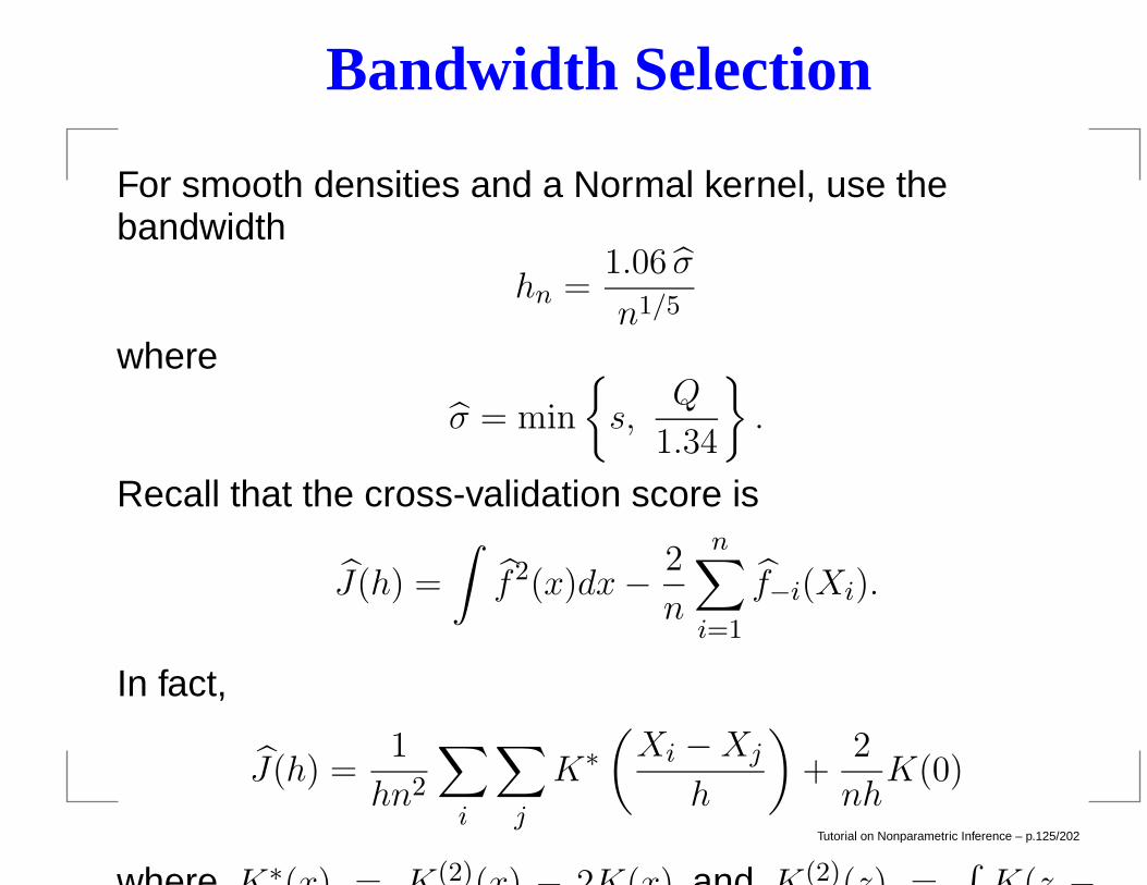
Bandwidth Selection
For smooth densities and a Normal kernel, use thebandwidth
hn =1.06 σ
n1/5
where
σ = min
s,
Q
1.34
.
Recall that the cross-validation score is
J(h) =
∫f2(x)dx− 2
n
n∑
i=1
f−i(Xi).
In fact,
J(h) =1
hn2
∑
i
∑
j
K∗
(Xi −Xj
h
)+
2
nhK(0)
where K∗(x) = K(2)(x) − 2K(x) and K(2)(z) =∫K(z −
y)K(y)dy.
Tutorial on Nonparametric Inference – p.125/202
Density Estimation with R
See hist() to make histogramsSee density() for kernel density estimator andbw.nrd() for bandwidth selection.
Tutorial on Nonparametric Inference – p.126/202
Measurement Error
Suppose we are interested in regressing the outcome Y ona covariate X but we cannot observe X directly. Rather, weobserve X plus noise U .
The observed data are (X?1 , Y1), . . . , (X
?n, Yn) where
Yi = f(Xi) + εi
X?i = Xi + Ui, E(Ui) = 0.
This is called a measurement error problem or anerrors-in-variables problem.
It is tempting to ignore the error and just regress Y on X?
but this leads to inconsistent estimates of f(x).
Tutorial on Nonparametric Inference – p.127/202
Measurement Error
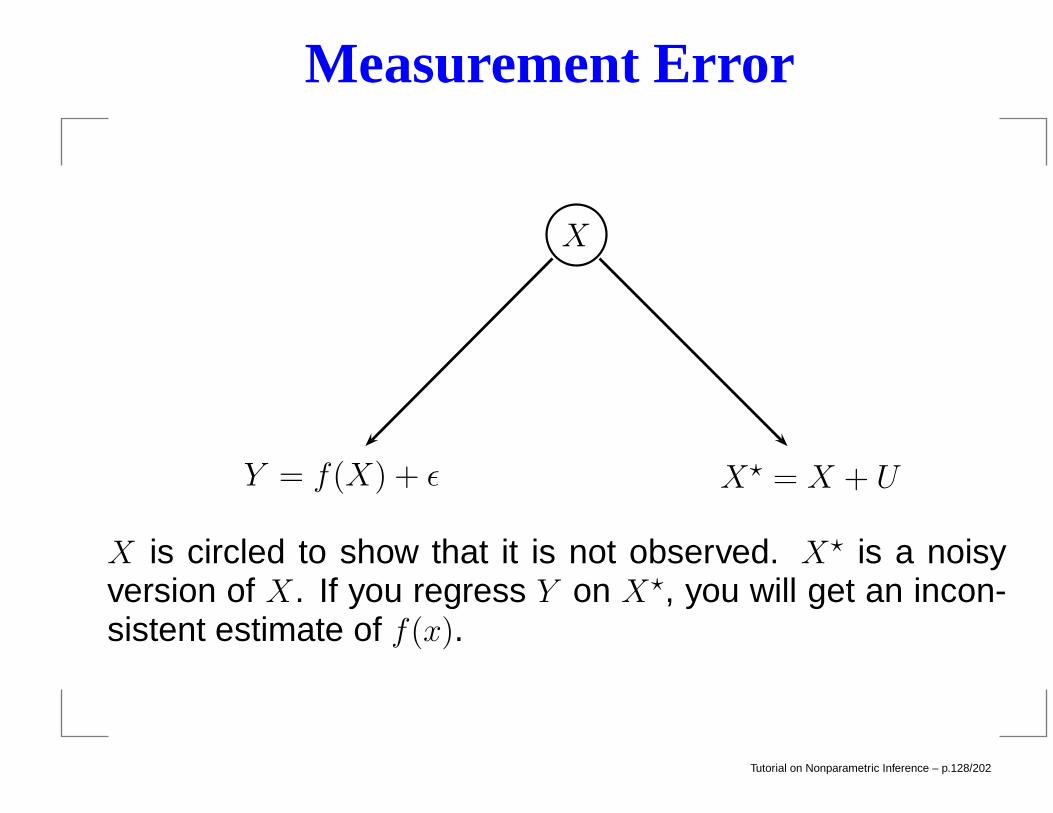
Y = f(X) + ε
X
X? = X + U
X is circled to show that it is not observed. X? is a noisyversion of X. If you regress Y on X?, you will get an incon-sistent estimate of f(x).
Tutorial on Nonparametric Inference – p.128/202
Measurement Error
Start with linear regression. The model is
Yi = β0 + β1Xi + εi
X?i = Xi + Ui.
Let β1 be the least squares estimator of β1 obtained byregressing the Yi’s on the X?
i ’s. Then
βas→ λβ1
where λ = σ2x
σ2x+σ2
u< 1.
This is called attenuation bias.
Tutorial on Nonparametric Inference – p.129/202
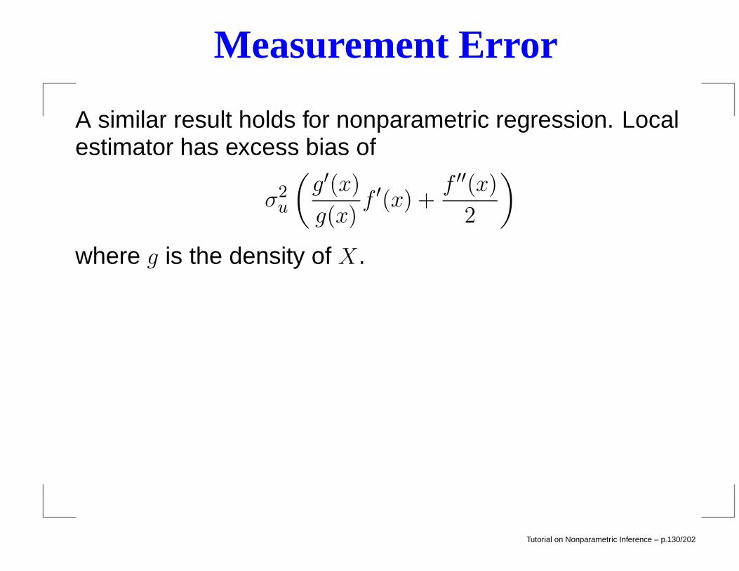
Measurement Error
A similar result holds for nonparametric regression. Localestimator has excess bias of
σ2u
(g′(x)
g(x)f ′(x) +
f ′′(x)
2
)
where g is the density of X.
Tutorial on Nonparametric Inference – p.130/202
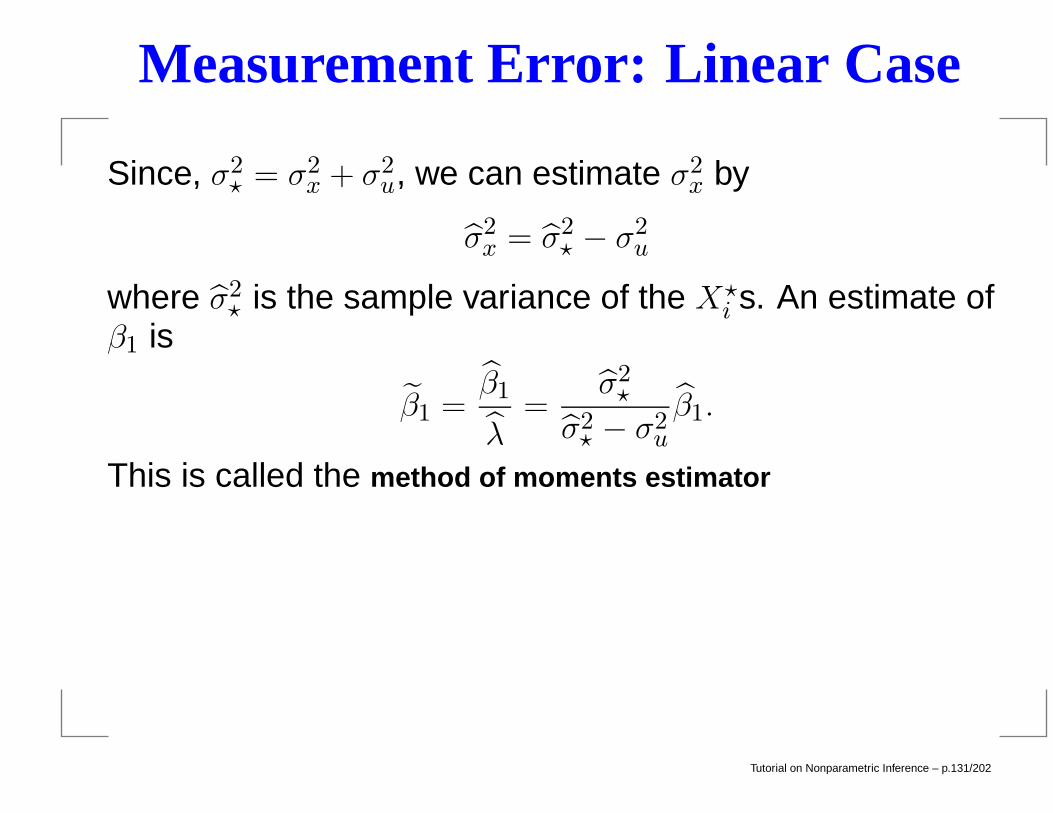
Measurement Error: Linear Case
Since, σ2? = σ2
x + σ2u, we can estimate σ2
x by
σ2x = σ2
? − σ2u
where σ2? is the sample variance of the X?
i s. An estimate ofβ1 is
β1 =β1
λ=
σ2?
σ2? − σ2
uβ1.
This is called the method of moments estimator
Tutorial on Nonparametric Inference – p.131/202
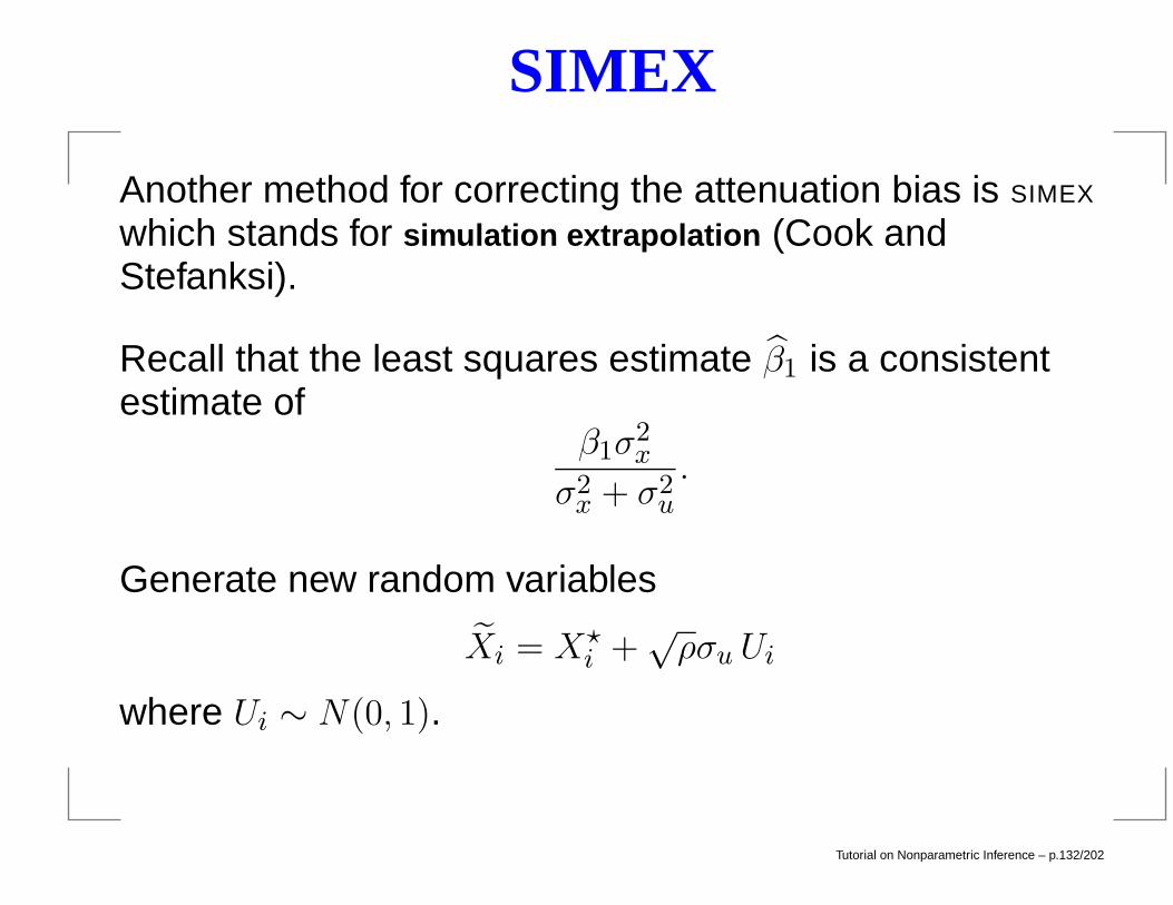
SIMEX
Another method for correcting the attenuation bias is SIMEX
which stands for simulation extrapolation (Cook andStefanksi).
Recall that the least squares estimate β1 is a consistentestimate of
β1σ2x
σ2x + σ2
u.
Generate new random variables
Xi = X?i +√ρσu Ui
where Ui ∼ N(0, 1).
Tutorial on Nonparametric Inference – p.132/202
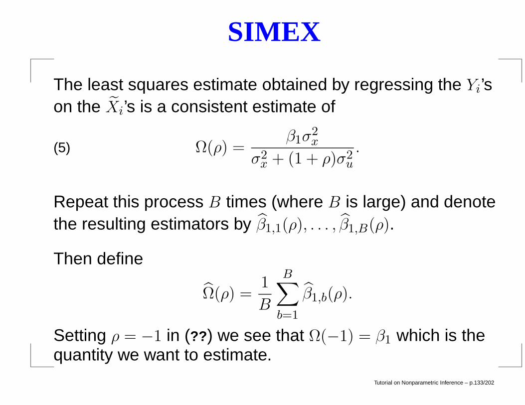
SIMEX
The least squares estimate obtained by regressing the Yi’son the Xi’s is a consistent estimate of
Ω(ρ) =β1σ
2x
σ2x + (1 + ρ)σ2
u.(5)
Repeat this process B times (where B is large) and denotethe resulting estimators by β1,1(ρ), . . . , β1,B(ρ).
Then define
Ω(ρ) =1
B
B∑
b=1
β1,b(ρ).
Setting ρ = −1 in (??) we see that Ω(−1) = β1 which is thequantity we want to estimate.
Tutorial on Nonparametric Inference – p.133/202
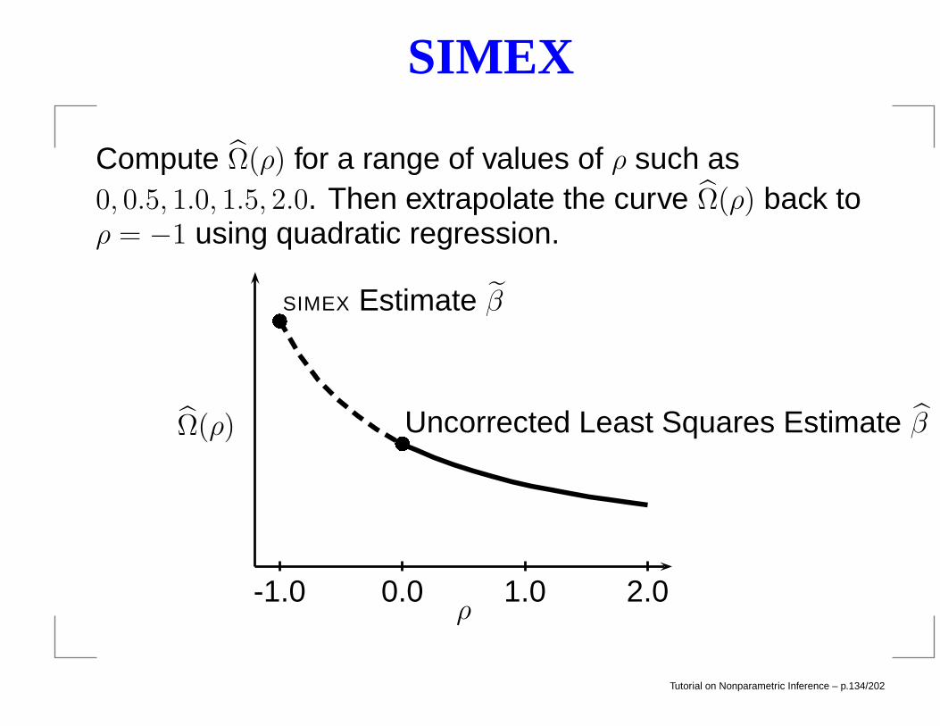
SIMEX
Compute Ω(ρ) for a range of values of ρ such as0, 0.5, 1.0, 1.5, 2.0. Then extrapolate the curve Ω(ρ) back toρ = −1 using quadratic regression.
-1.0 0.0 1.0 2.0ρ
Uncorrected Least Squares Estimate β
SIMEX Estimate β
Ω(ρ)
Tutorial on Nonparametric Inference – p.134/202
Nonparametric Case
An advantage of SIMEX is that it extends readily tononparametric regression. Let fn(x) be an uncorrectedestimate of f(x) obtained by regressing the Yi’s on the X?
i ’sin the nonparametric problem
Yi = f(Xi) + εi
X?i = Xi + Ui.
Now perform the simex algorithm to get fn(x, ρ) and definethe corrected estimator fn(x) = fn(x,−1).
Tutorial on Nonparametric Inference – p.135/202
Nonparametric Case
A more direct way to deal with measurement error issuggested by Fan and Truong. They propose the kernelestimator
fn(x) =
∑ni=1Kn
(x−X?
i
hn
)Yi
∑ni=1Kn
(x−X?
i
hn
)
where
Kn(x) =1
2π
∫e−itx
φK(t)
φU (t/hn)dt,
where φK is the Fourier transform of a kernel K and φU isthe characteristic function of U .
Tutorial on Nonparametric Inference – p.136/202
Nonparametric Case
Yet another way. Write the uncorrected estimator as
fn(x) =n∑
i=1
Yi `i(x,X?i ).
If the Xi’s had been observed, the estimator of r would be
f∗n(x) =
n∑
i=1
Yi `i(x,Xi).
Expanding `i(x,X?i ) around Xi we have
fn(x) ≈ f∗
n(x) +n∑
i=1
Yi(X?i −Xi)`
′(x,Xi) +1
2
n∑
i=1
Yi(X?i −Xi)
2`′′(x,Xi).
Tutorial on Nonparametric Inference – p.137/202
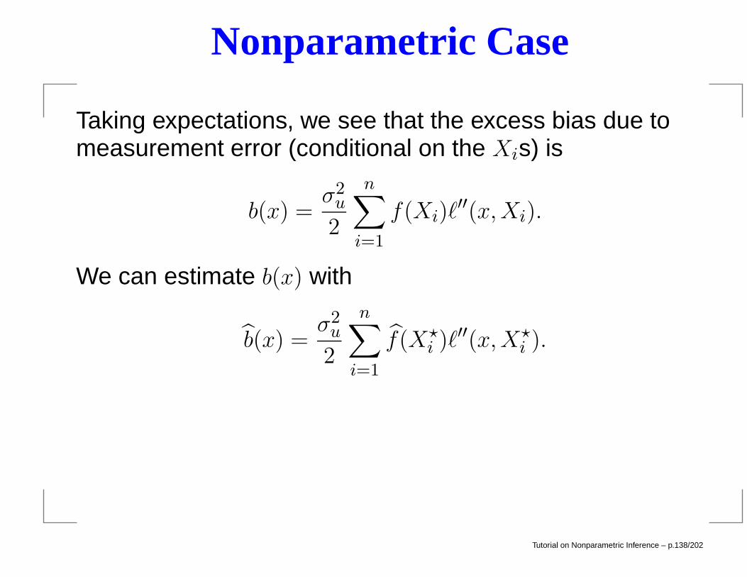
Nonparametric Case
Taking expectations, we see that the excess bias due tomeasurement error (conditional on the Xis) is
b(x) =σ2u
2
n∑
i=1
f(Xi)`′′(x,Xi).
We can estimate b(x) with
b(x) =σ2u
2
n∑
i=1
f(X?i )`
′′(x,X?i ).
Tutorial on Nonparametric Inference – p.138/202
Example
The function locfitsimex() allows you to estimate f(x)via local linearusing SIMEX to correct for bias due tomeasurement error.
> locfitsimex(xerr, y, measerrvar, simexreps, h, deg=deg)
This function returns a matrix.
Rows correspond to ρ = 0, 0.5, 1, 1.5, 2,−1.
Columns are the fit evaluated at 100 X values ranging frommin(xerr) to max(xerr), i.e.
> seq(min(xerr),max(xerr),length=100)
Tutorial on Nonparametric Inference – p.139/202
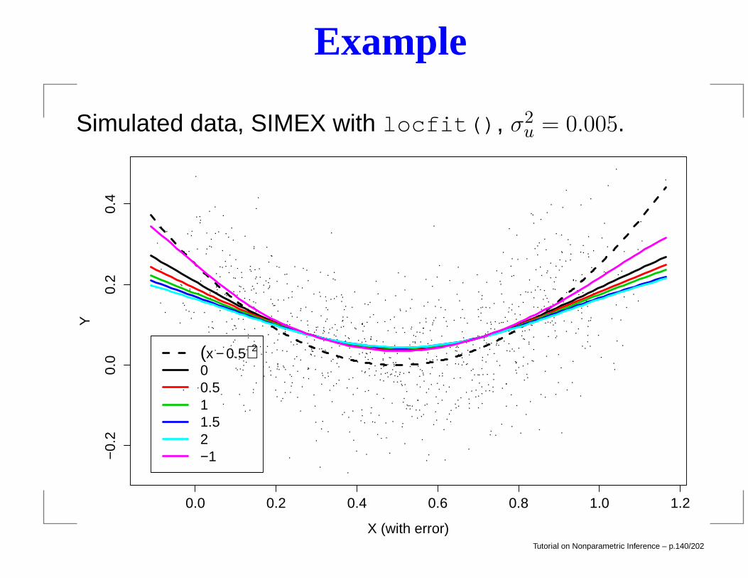
Example
Simulated data, SIMEX with locfit(), σ2u = 0.005.
0.0 0.2 0.4 0.6 0.8 1.0 1.2
−0.
20.
00.
20.
4
X (with error)
Y
(x − 0.5)2
00.511.52−1
Tutorial on Nonparametric Inference – p.140/202
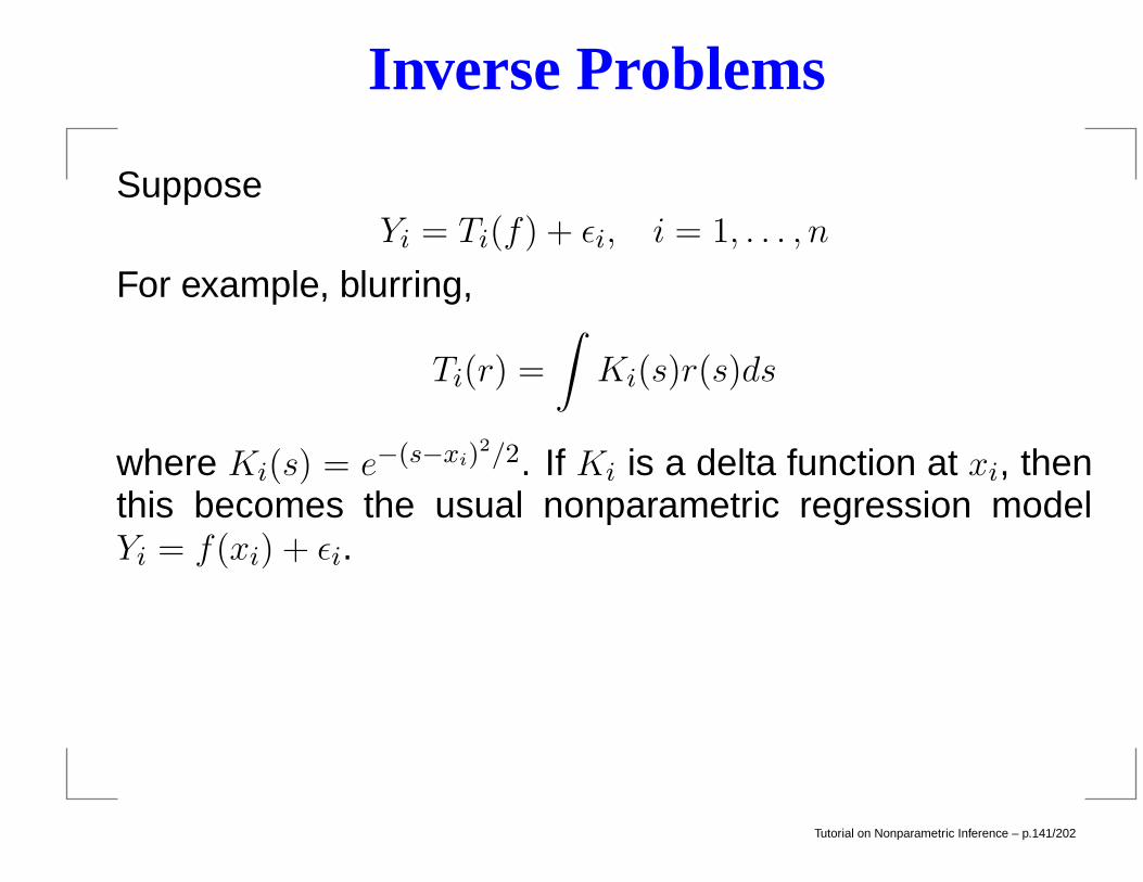
Inverse Problems
SupposeYi = Ti(f) + εi, i = 1, . . . , n
For example, blurring,
Ti(r) =
∫Ki(s)r(s)ds
where Ki(s) = e−(s−xi)2/2. If Ki is a delta function at xi, then
this becomes the usual nonparametric regression modelYi = f(xi) + εi.
Tutorial on Nonparametric Inference – p.141/202
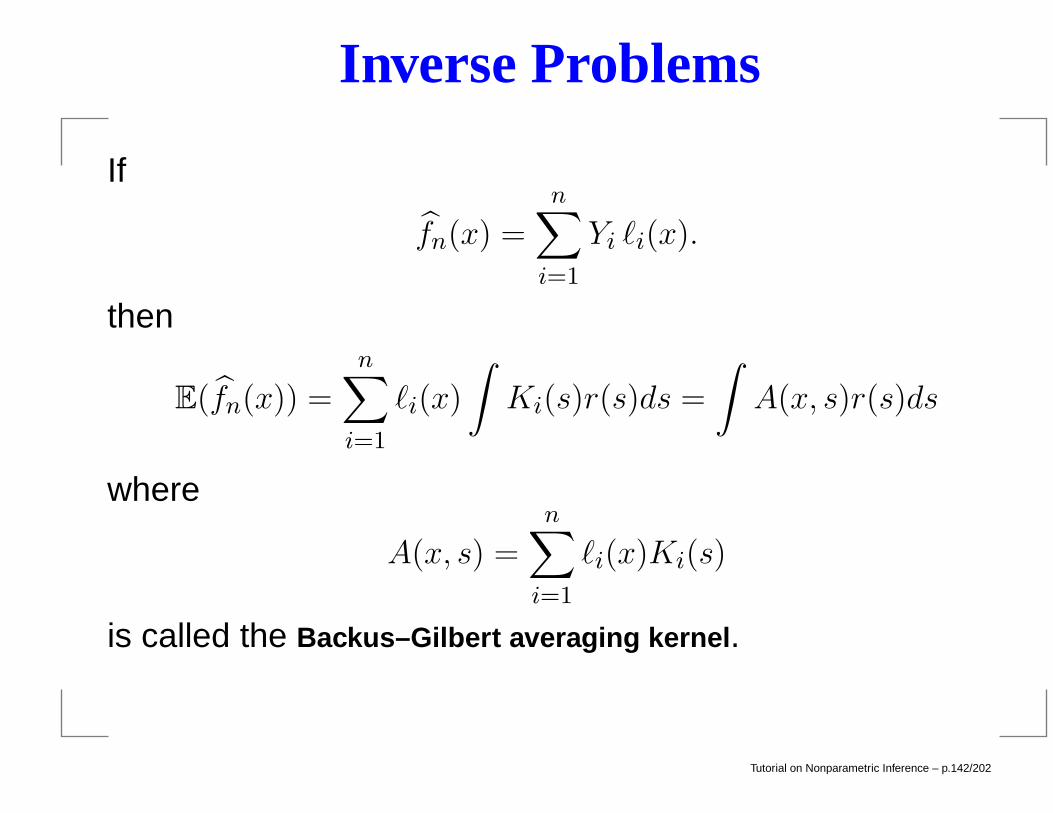
Inverse Problems
If
fn(x) =
n∑
i=1
Yi `i(x).
then
E(fn(x)) =
n∑
i=1
`i(x)
∫Ki(s)r(s)ds =
∫A(x, s)r(s)ds
where
A(x, s) =
n∑
i=1
`i(x)Ki(s)
is called the Backus–Gilbert averaging kernel.
Tutorial on Nonparametric Inference – p.142/202
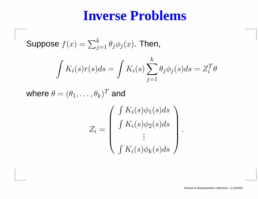
Inverse Problems
Suppose f(x) =∑k
j=1 θjφj(x). Then,
∫Ki(s)r(s)ds =
∫Ki(s)
k∑
j=1
θjφj(s)ds = ZTi θ
where θ = (θ1, . . . , θk)T and
Zi =
∫Ki(s)φ1(s)ds
∫Ki(s)φ2(s)ds
...∫Ki(s)φk(s)ds
.
Tutorial on Nonparametric Inference – p.143/202
Inverse Problems
The model can then be written as
Y = Zθ + ε
where Z is an n× k matrix with ith row equal to ZTi ,Y = (Y1, . . . , Yn)
T and ε = (ε1, . . . , εn)T .
It is tempting to estimate θ by the least squares estimator(ZTZ)−1ZTY . This may fail since ZTZ is typically notinvertible in which case the problem is said to be ill-posed.
This is a hallmark of inverse problems: The function f can-not be recovered, even in the absence of noise, due to theinformation loss incurred by blurring.
Tutorial on Nonparametric Inference – p.144/202
Inverse Problems
Instead, it is common to use a regularized estimator suchas θ = LY where
L = (ZTZ + λI)−1ZT ,
I is the identity matrix and λ > 0 is a smoothing parameterthat can be chosen by cross-validation.
Note that cross-validation is estimating the prediction error
n−1n∑
i=1
(
∫Ki(s)r(s)ds−
∫Ki(s)r(s)ds)
2
rather than ∫(r(s)− r(s))2ds.
Tutorial on Nonparametric Inference – p.145/202
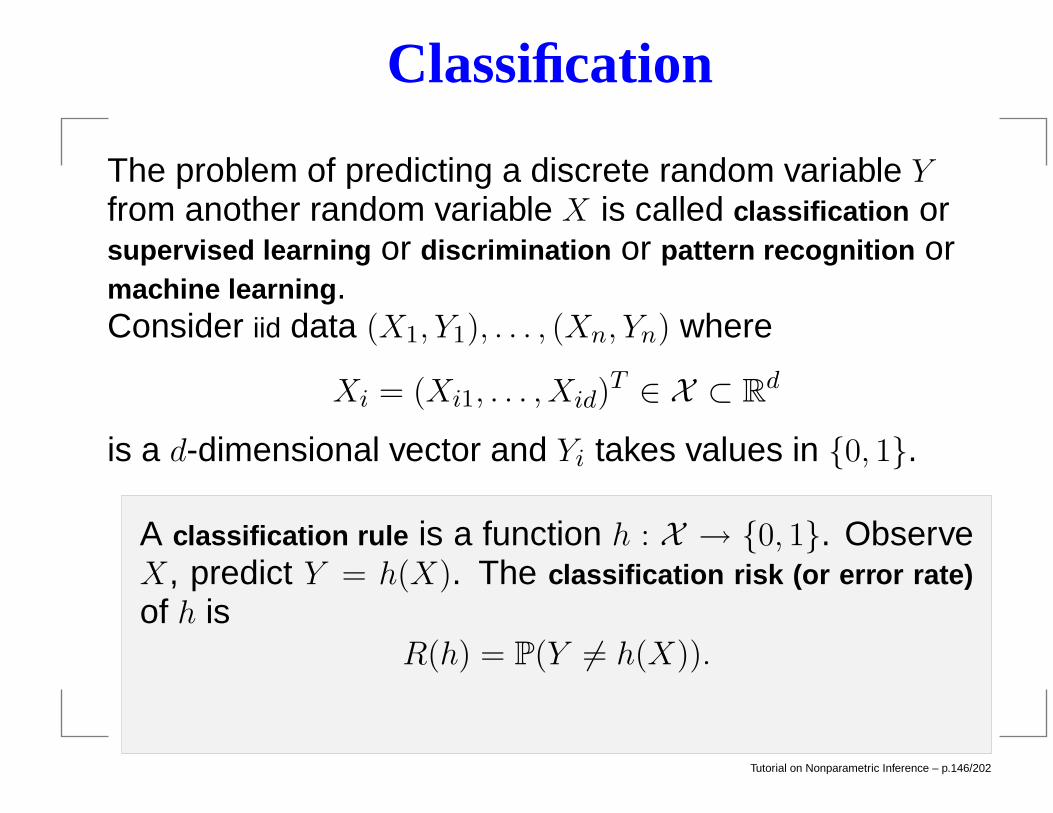
Classification
The problem of predicting a discrete random variable Yfrom another random variable X is called classification orsupervised learning or discrimination or pattern recognition ormachine learning.Consider iid data (X1, Y1), . . . , (Xn, Yn) where
Xi = (Xi1, . . . , Xid)T ∈ X ⊂ R
d
is a d-dimensional vector and Yi takes values in 0, 1.
A classification rule is a function h : X → 0, 1. ObserveX, predict Y = h(X). The classification risk (or error rate)of h is
R(h) = P(Y 6= h(X)).
Tutorial on Nonparametric Inference – p.146/202
Classification
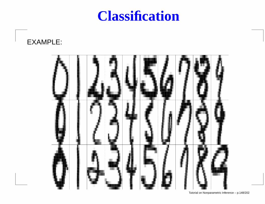
EXAMPLE:Identify handwritten digits from images. Each Y is a digitfrom 0 to 9. There are 256 covariates x1, . . . , x256
corresponding to the intensity values from the pixels of the16 X 16 image.
Tutorial on Nonparametric Inference – p.147/202
Classification
EXAMPLE:
Tutorial on Nonparametric Inference – p.148/202
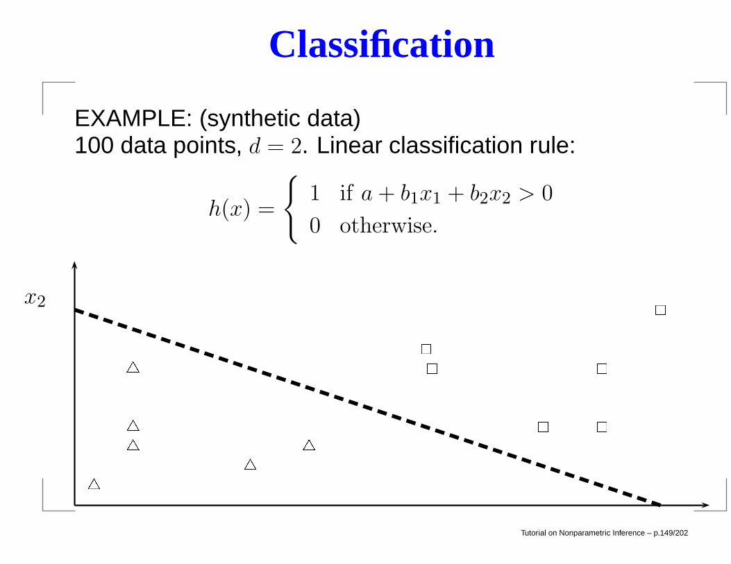
Classification
EXAMPLE: (synthetic data)100 data points, d = 2. Linear classification rule:
h(x) =
1 if a+ b1x1 + b2x2 > 0
0 otherwise.
x1
x2
Tutorial on Nonparametric Inference – p.149/202
Error Rates
The true error rate (or classification risk) of a classifier h is
R(h) = P(h(X) 6= Y )and the empirical error rate or training error rate is
Rn(h) =1
n
n∑
i=1
I(h(Xi) 6= Yi).
Tutorial on Nonparametric Inference – p.150/202
The Bayes Rule
The rule h that minimizes R(h) is
h∗(x) =
1 if r(x) > 1
2
0 otherwise
wherer(x) = E(Y |X = x) = P(Y = 1|X = x)
denote the regression function. The rule h∗ is called theBayes’ rule. Note: the Bayes rule has nothing to do withBayesian inferencd. The set
D(h) = x : r(x) = 1/2is called the decision boundary.
Tutorial on Nonparametric Inference – p.151/202
Three Approaches
1. Empirical Risk Minimization Choose a set of classifiers Hand find h ∈ H that minimizes some estimate of L(h).
2. Regression. Find an estimate r of the regression functionr and substitute into the Bayes rule.
3. Density Estimation. Estimate f0 from the Xi’s for whichYi = 0, estimate f1 from the Xi’s for which Yi = 1 and letπ = n−1
∑ni=1 Yi. Define
r(x) = P(Y = 1|X = x) =πf1(x)
πf1(x) + (1− π)f0(x)
and
h(x) =
1 if r(x) > 1
2
0 otherwise.
Tutorial on Nonparametric Inference – p.152/202
Linear and Logistic Regression
Regression approach is to estimater(x) = E(Y |X = x) = P(Y = 1|X = x). Can use linear
Y = r(x) + ε = β0 +d∑
j=1
βjXj + ε
or logistic
r(x) = P(Y = 1|X = x) =eβ0+
∑jβjxj
1 + eβ0+∑
jβjxj
.
Even if the model is wrong this might work well since we onlyneed to approximate the decision boundary.
Tutorial on Nonparametric Inference – p.153/202
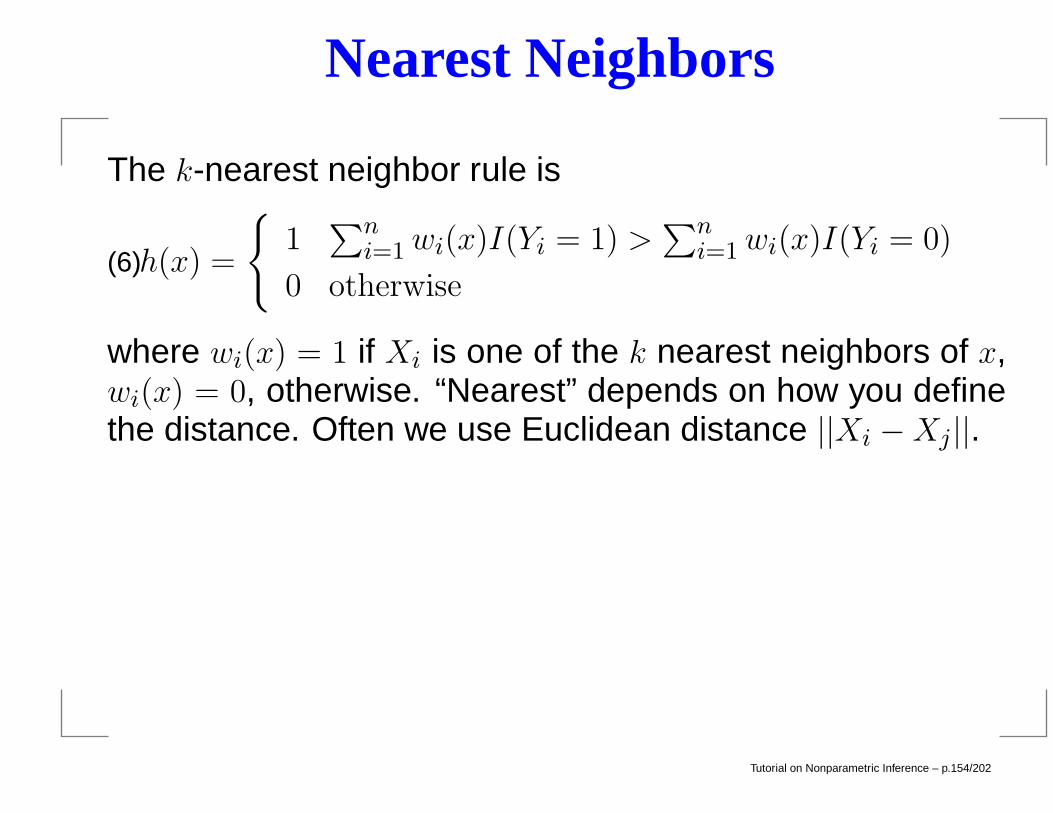
Nearest Neighbors
The k-nearest neighbor rule is
h(x) =
1∑n
i=1wi(x)I(Yi = 1) >∑n
i=1wi(x)I(Yi = 0)
0 otherwise(6)
where wi(x) = 1 if Xi is one of the k nearest neighbors of x,wi(x) = 0, otherwise. “Nearest” depends on how you definethe distance. Often we use Euclidean distance ||Xi −Xj ||.
Tutorial on Nonparametric Inference – p.154/202
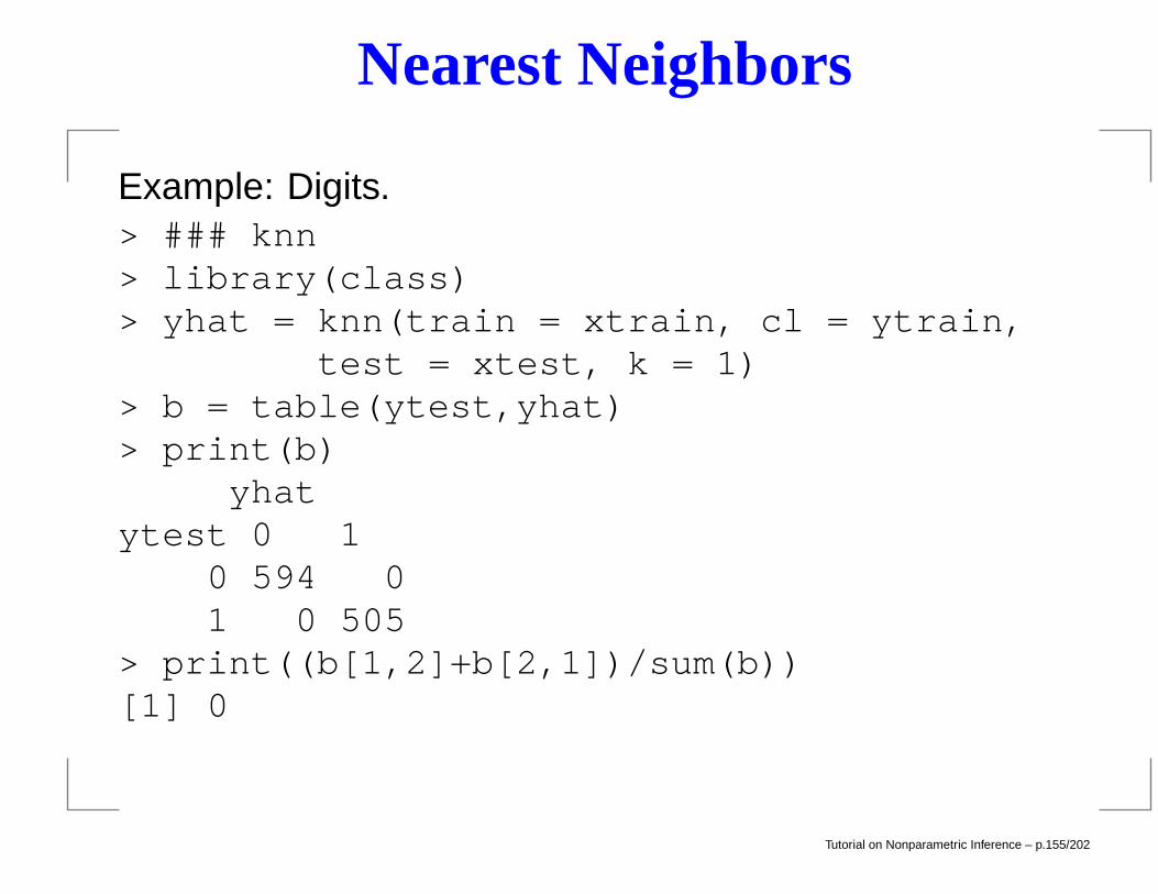
Nearest Neighbors
Example: Digits.> ### knn> library(class)> yhat = knn(train = xtrain, cl = ytrain,
test = xtest, k = 1)> b = table(ytest,yhat)> print(b)
yhatytest 0 1
0 594 01 0 505
> print((b[1,2]+b[2,1])/sum(b))[1] 0
Tutorial on Nonparametric Inference – p.155/202
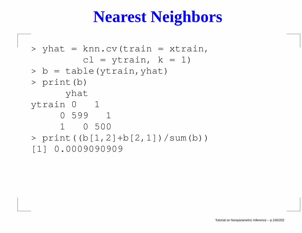
Nearest Neighbors
> yhat = knn.cv(train = xtrain,cl = ytrain, k = 1)
> b = table(ytrain,yhat)> print(b)
yhatytrain 0 1
0 599 11 0 500
> print((b[1,2]+b[2,1])/sum(b))[1] 0.0009090909
Tutorial on Nonparametric Inference – p.156/202
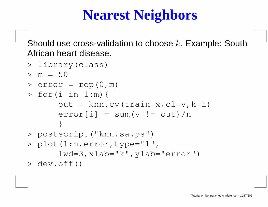
Nearest Neighbors
Should use cross-validation to choose k. Example: SouthAfrican heart disease.> library(class)> m = 50> error = rep(0,m)> for(i in 1:m)
out = knn.cv(train=x,cl=y,k=i)error[i] = sum(y != out)/n
> postscript("knn.sa.ps")> plot(1:m,error,type="l",
lwd=3,xlab="k",ylab="error")> dev.off()
Tutorial on Nonparametric Inference – p.157/202
Nearest Neighbors
0 10 20 30 40 50
−1.
0−
0.5
0.0
0.5
1.0
k
erro
r
Tutorial on Nonparametric Inference – p.158/202
Gaussian, Linear and Quadratic Classifiers
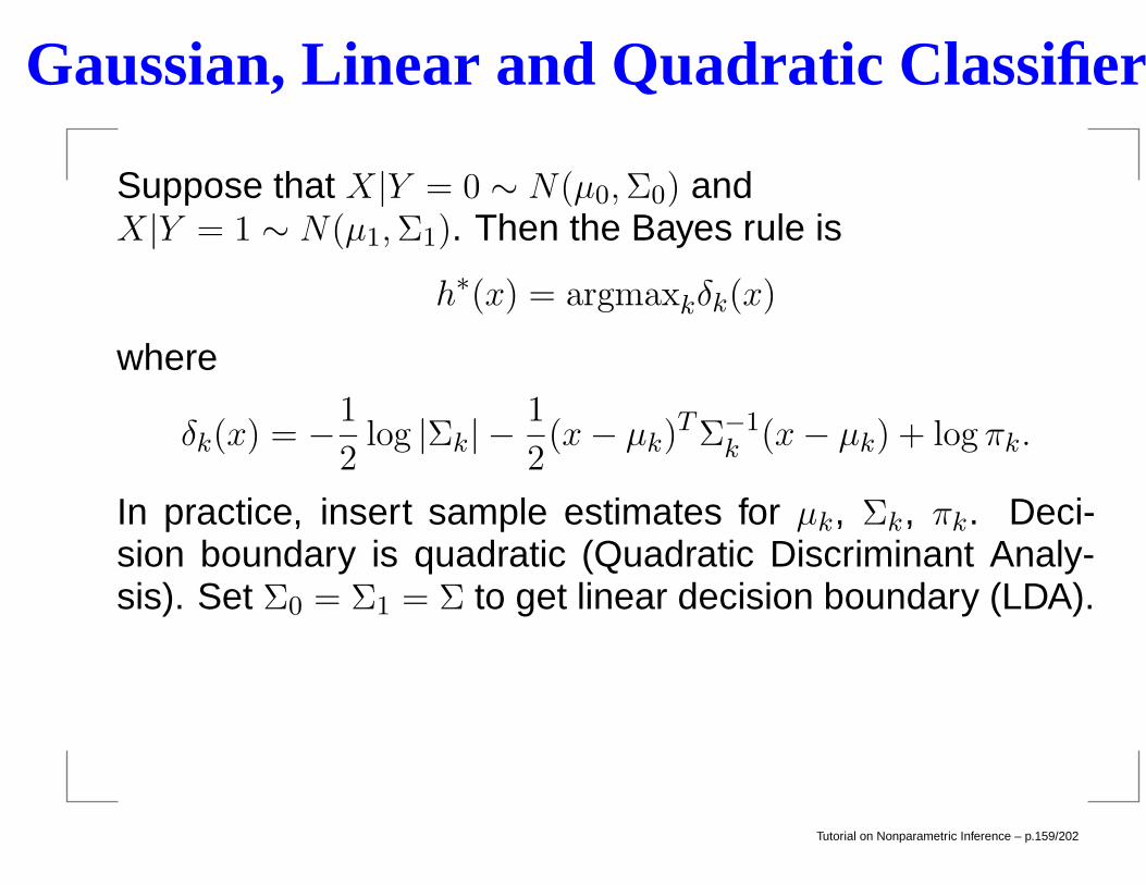
Suppose that X|Y = 0 ∼ N(µ0,Σ0) andX|Y = 1 ∼ N(µ1,Σ1). Then the Bayes rule is
h∗(x) = argmaxkδk(x)
where
δk(x) = −1
2log |Σk| −
1
2(x− µk)TΣ−1
k (x− µk) + log πk.
In practice, insert sample estimates for µk, Σk, πk. Deci-sion boundary is quadratic (Quadratic Discriminant Analy-sis). Set Σ0 = Σ1 = Σ to get linear decision boundary (LDA).
Tutorial on Nonparametric Inference – p.159/202
Example
South African heart disease data. In R use:> out = lda(x,y) ### or qda for quadratic> yhat = predict(out)$classThe error rate of LDA is .25. For QDA we get .24. In thisexample, there is little advantage to QDA over LDA.
Tutorial on Nonparametric Inference – p.160/202
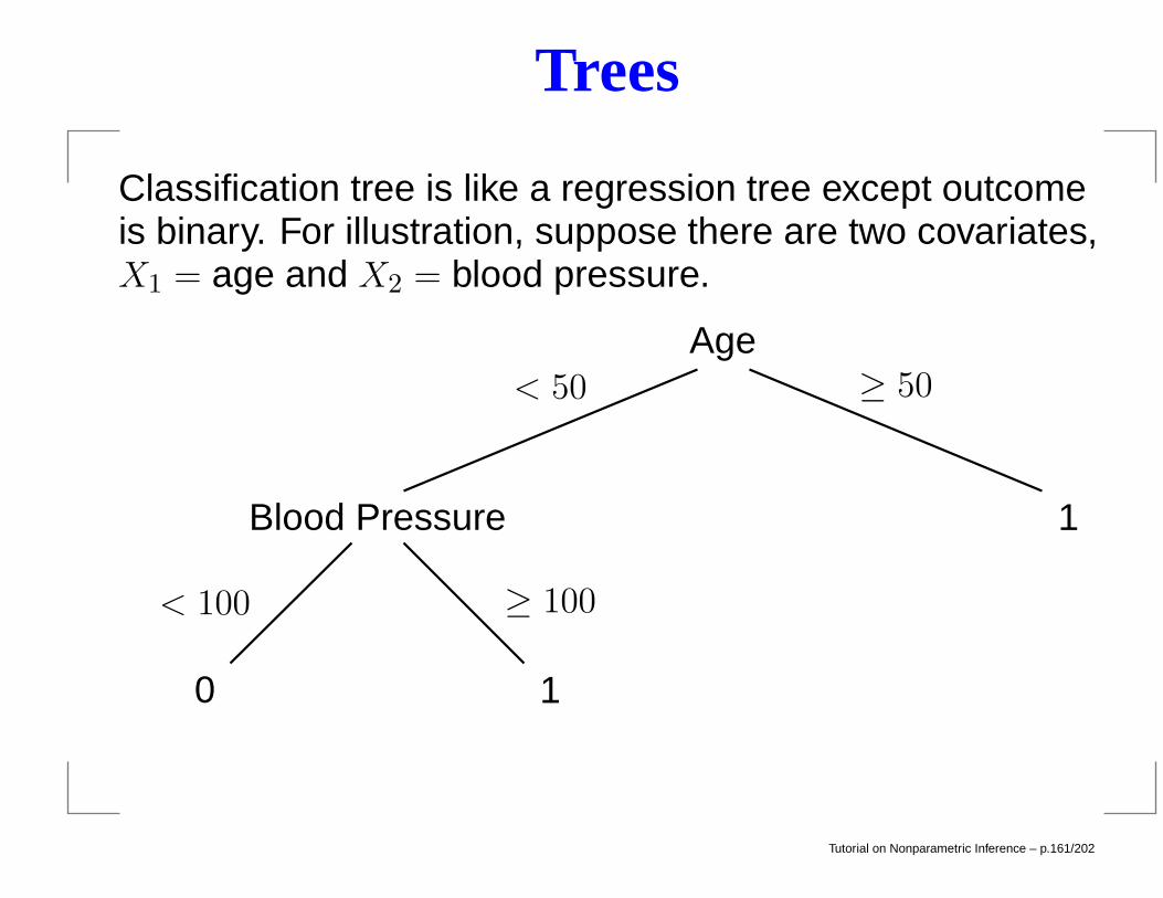
Trees
Classification tree is like a regression tree except outcomeis binary. For illustration, suppose there are two covariates,X1 = age and X2 = blood pressure.
0 1
Blood Pressure 1
Age
< 100 ≥ 100
< 50 ≥ 50
Tutorial on Nonparametric Inference – p.161/202
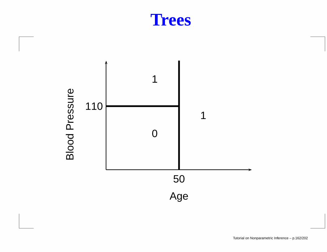
Trees
1
0
1
Age
Blo
odP
ress
ure
50
110
Tutorial on Nonparametric Inference – p.162/202
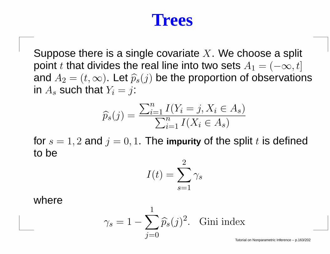
Trees
Suppose there is a single covariate X. We choose a splitpoint t that divides the real line into two sets A1 = (−∞, t]and A2 = (t,∞). Let ps(j) be the proportion of observationsin As such that Yi = j:
ps(j) =
∑ni=1 I(Yi = j,Xi ∈ As)∑n
i=1 I(Xi ∈ As)for s = 1, 2 and j = 0, 1. The impurity of the split t is definedto be
I(t) =
2∑
s=1
γs
where
γs = 1−1∑
j=0
ps(j)2. Gini index
Tutorial on Nonparametric Inference – p.163/202
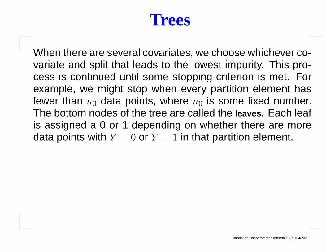
Trees
When there are several covariates, we choose whichever co-variate and split that leads to the lowest impurity. This pro-cess is continued until some stopping criterion is met. Forexample, we might stop when every partition element hasfewer than n0 data points, where n0 is some fixed number.The bottom nodes of the tree are called the leaves. Each leafis assigned a 0 or 1 depending on whether there are moredata points with Y = 0 or Y = 1 in that partition element.
Tutorial on Nonparametric Inference – p.164/202
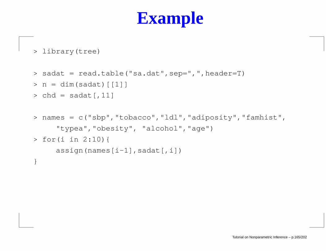
Example
> library(tree)
> sadat = read.table("sa.dat",sep=",",header=T)
> n = dim(sadat)[[1]]
> chd = sadat[,11]
> names = c("sbp","tobacco","ldl","adiposity","famhist",
"typea","obesity", "alcohol","age")
> for(i in 2:10)
assign(names[i-1],sadat[,i])
Tutorial on Nonparametric Inference – p.165/202
Example
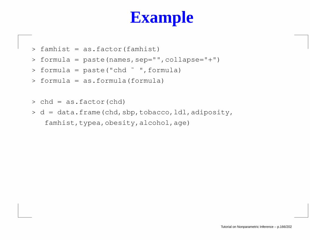
> famhist = as.factor(famhist)
> formula = paste(names,sep="",collapse="+")
> formula = paste("chd ˜ ",formula)
> formula = as.formula(formula)
> chd = as.factor(chd)
> d = data.frame(chd,sbp,tobacco,ldl,adiposity,
famhist,typea,obesity,alcohol,age)
Tutorial on Nonparametric Inference – p.166/202
Example
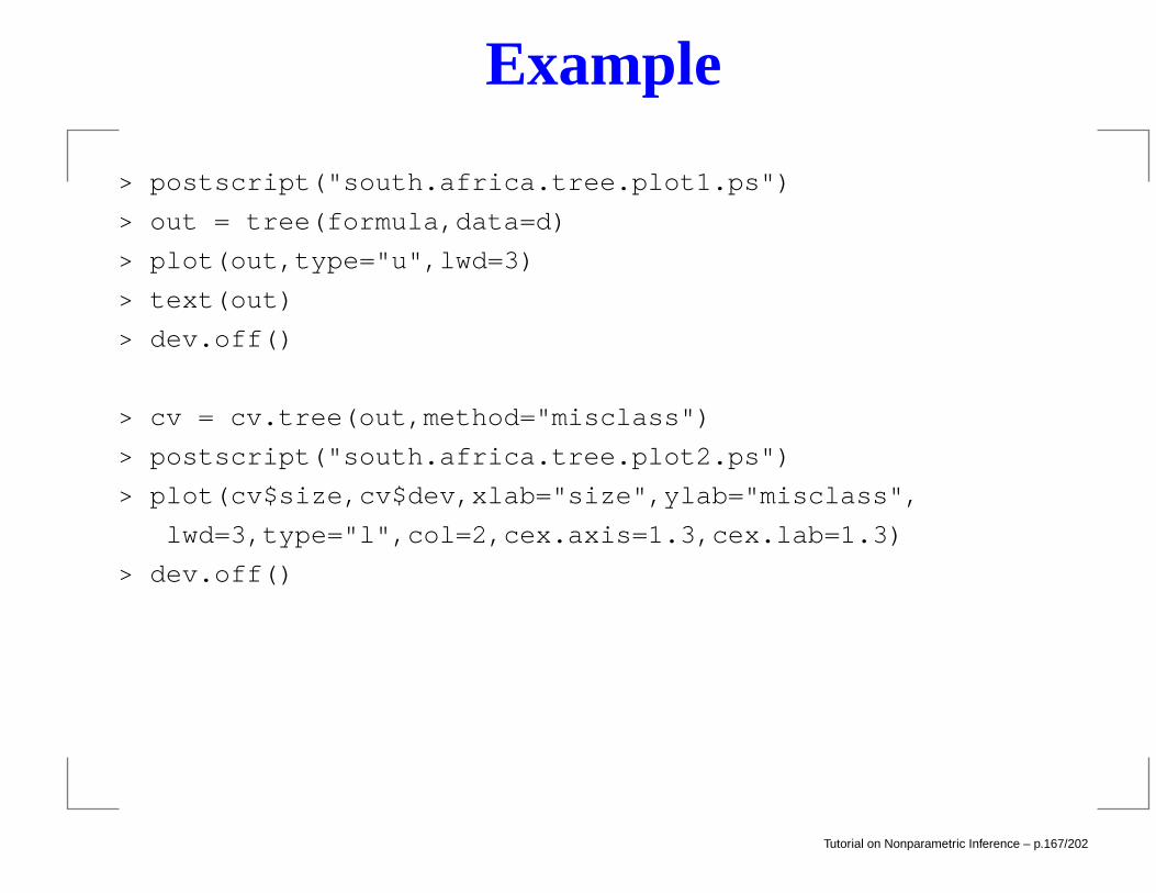
> postscript("south.africa.tree.plot1.ps")
> out = tree(formula,data=d)
> plot(out,type="u",lwd=3)
> text(out)
> dev.off()
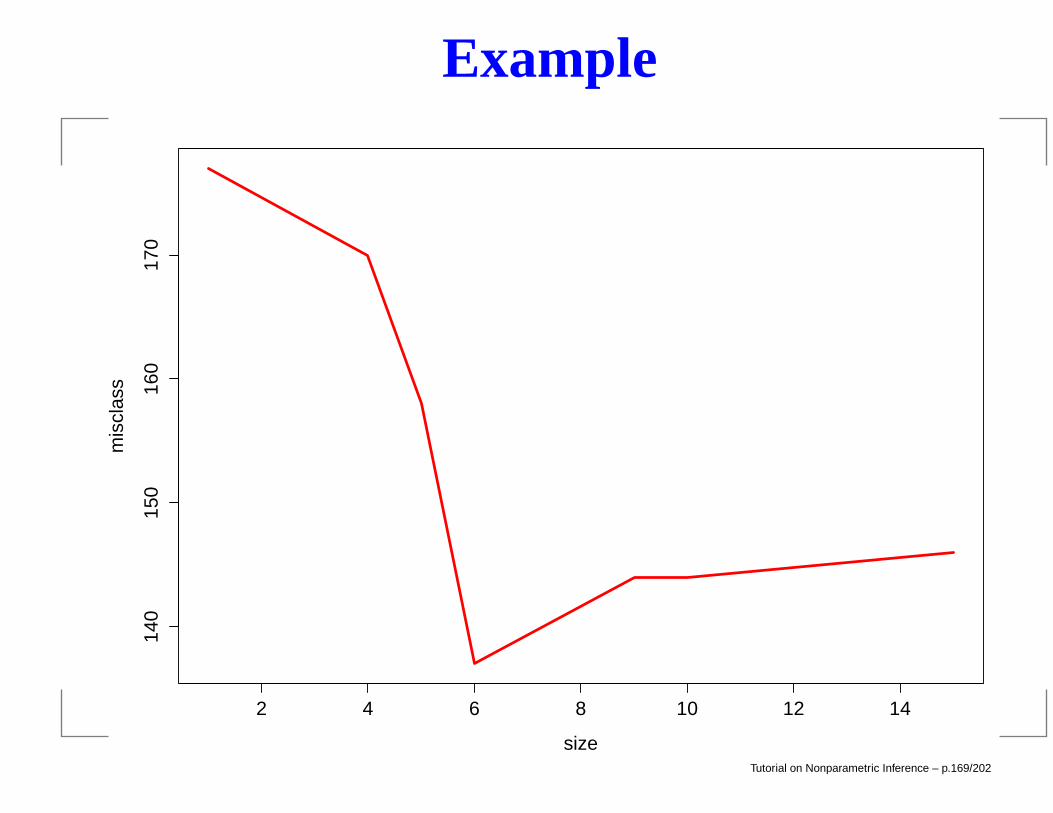
> cv = cv.tree(out,method="misclass")
> postscript("south.africa.tree.plot2.ps")
> plot(cv$size,cv$dev,xlab="size",ylab="misclass",
lwd=3,type="l",col=2,cex.axis=1.3,cex.lab=1.3)
> dev.off()
Tutorial on Nonparametric Inference – p.167/202

Example
|age < 31.5
tobacco < 0.51
alcohol < 11.105
age < 50.5
typea < 68.5 famhist:a
tobacco < 7.605
typea < 42.5
adiposity < 24.435
adiposity < 28.955
ldl < 6.705
tobacco < 4.15
adiposity < 28
typea < 48
0
0 0 0 1
0
0 0
1 1
0 1
0
1
1
Tutorial on Nonparametric Inference – p.168/202
Example
2 4 6 8 10 12 14
140
150
160
170
size
mis
clas
s
Tutorial on Nonparametric Inference – p.169/202
Example
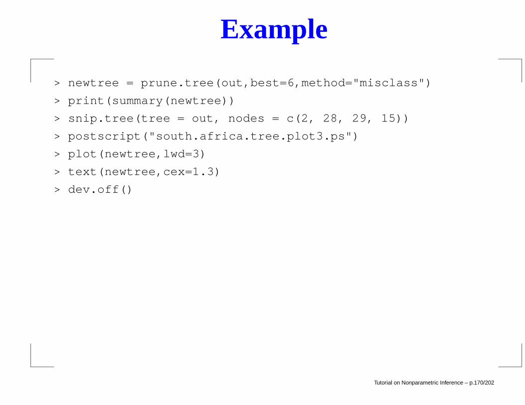
> newtree = prune.tree(out,best=6,method="misclass")
> print(summary(newtree))
> snip.tree(tree = out, nodes = c(2, 28, 29, 15))
> postscript("south.africa.tree.plot3.ps")
> plot(newtree,lwd=3)
> text(newtree,cex=1.3)
> dev.off()
Tutorial on Nonparametric Inference – p.170/202
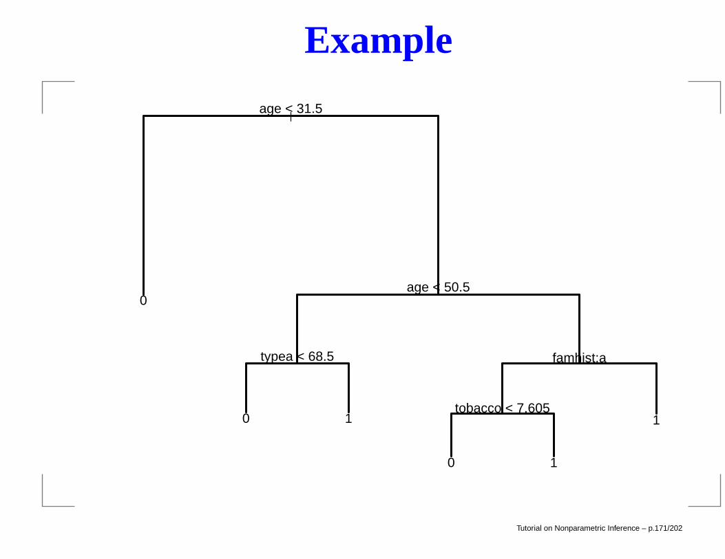
Example
|age < 31.5
age < 50.5
typea < 68.5 famhist:a
tobacco < 7.605
0
0 1
0 1
1
Tutorial on Nonparametric Inference – p.171/202
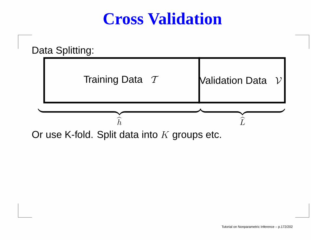
Cross Validation
Data Splitting:
Training Data T Validation Data V
︸ ︷︷ ︸h
︸ ︷︷ ︸L
Or use K-fold. Split data into K groups etc.
Tutorial on Nonparametric Inference – p.172/202
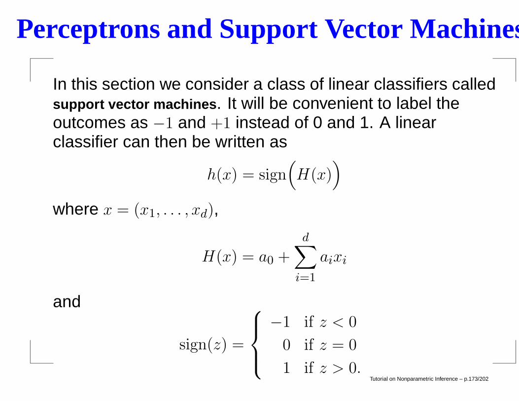
Perceptrons and Support Vector Machines
In this section we consider a class of linear classifiers calledsupport vector machines. It will be convenient to label theoutcomes as −1 and +1 instead of 0 and 1. A linearclassifier can then be written as
h(x) = sign(H(x)
)
where x = (x1, . . . , xd),
H(x) = a0 +
d∑
i=1
aixi
and
sign(z) =
−1 if z < 0
0 if z = 0
1 if z > 0.Tutorial on Nonparametric Inference – p.173/202
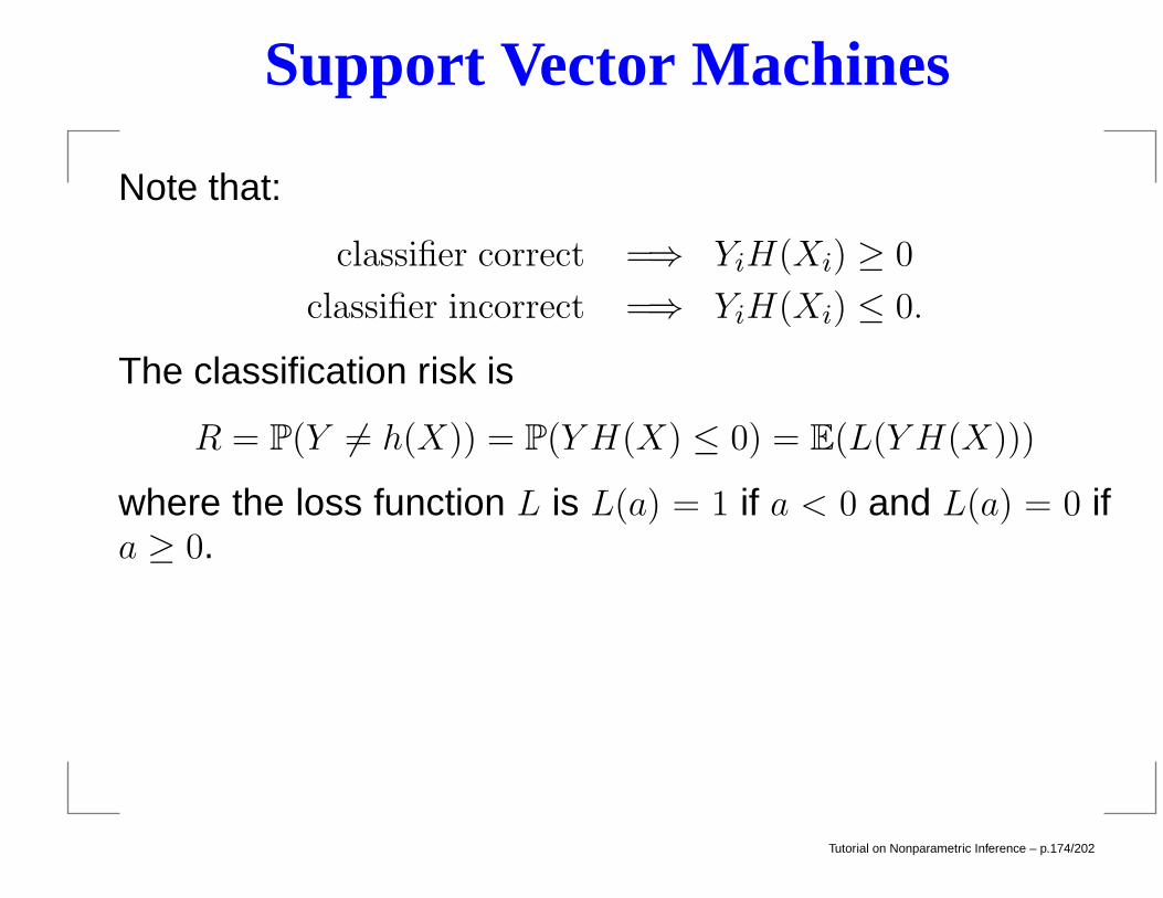
Support Vector Machines
Note that:
classifier correct =⇒ YiH(Xi) ≥ 0
classifier incorrect =⇒ YiH(Xi) ≤ 0.
The classification risk is
R = P(Y 6= h(X)) = P(Y H(X) ≤ 0) = E(L(Y H(X)))
where the loss function L is L(a) = 1 if a < 0 and L(a) = 0 ifa ≥ 0.
Tutorial on Nonparametric Inference – p.174/202
Support Vector Machines
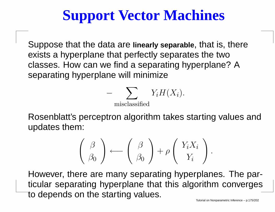
Suppose that the data are linearly separable, that is, thereexists a hyperplane that perfectly separates the twoclasses. How can we find a separating hyperplane? Aseparating hyperplane will minimize
−∑
misclassified
YiH(Xi).
Rosenblatt’s perceptron algorithm takes starting values andupdates them:
(β
β0
)←−
(β
β0
)+ ρ
(YiXi
Yi
).
However, there are many separating hyperplanes. The par-ticular separating hyperplane that this algorithm convergesto depends on the starting values.
Tutorial on Nonparametric Inference – p.175/202
Support Vector Machines
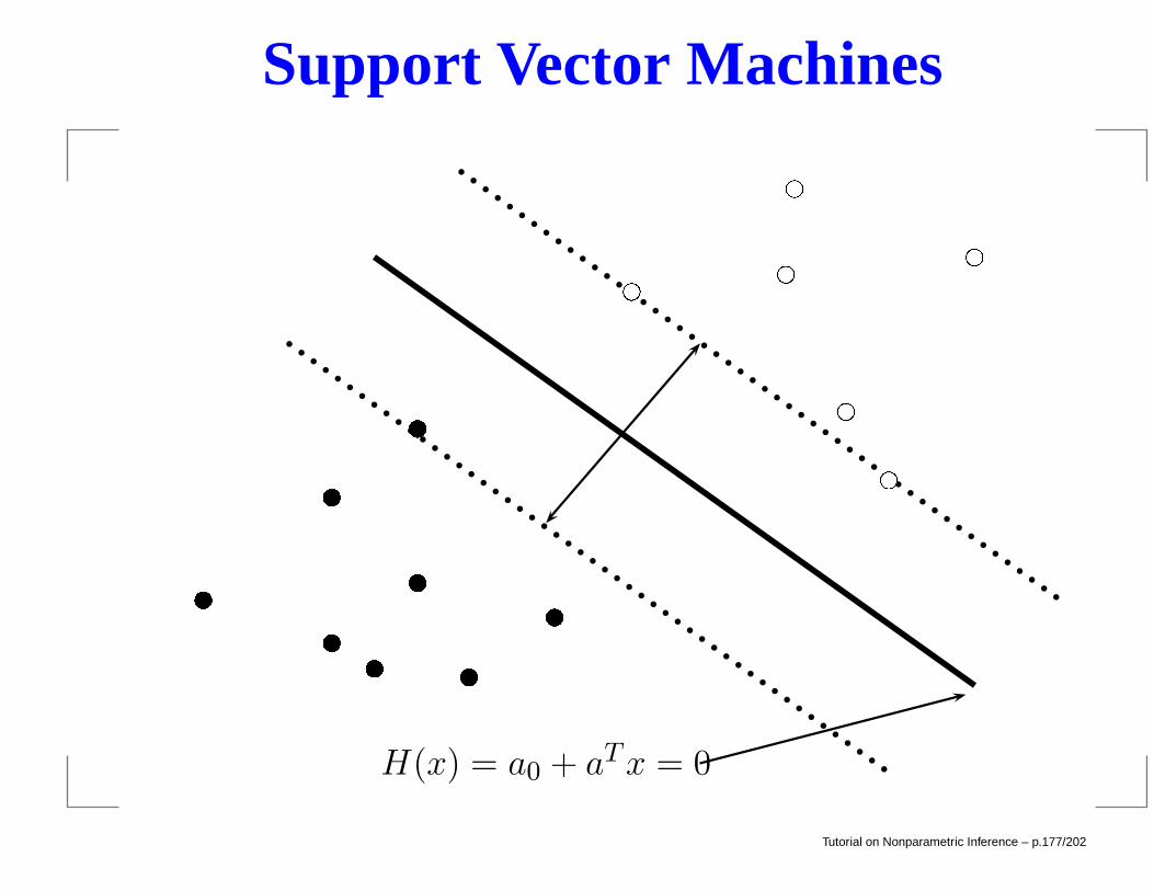
Intuitively, it seems reasonable to choose the hyperplane“furthest” from the data in the sense that it separates the+1s and -1s and maximizes the distance to the closest point.This hyperplane is called the maximum margin hyperplane. Themargin is the distance to from the hyperplane to the near-est point. Points on the boundary of the margin are calledsupport vectors.
Tutorial on Nonparametric Inference – p.176/202
Support Vector Machines
H(x) = a0 + aTx = 0
Tutorial on Nonparametric Inference – p.177/202
Support Vector Machines
The data can be separated by some hyperplane if and onlyif there exists a hyperplane H(x) = a0 +
∑di=1 aixi such that
YiH(xi) ≥ 1, i = 1, . . . , n.
The goal, then, is to maximize the margin, subject to thiscondition.
Tutorial on Nonparametric Inference – p.178/202
Support Vector Machines
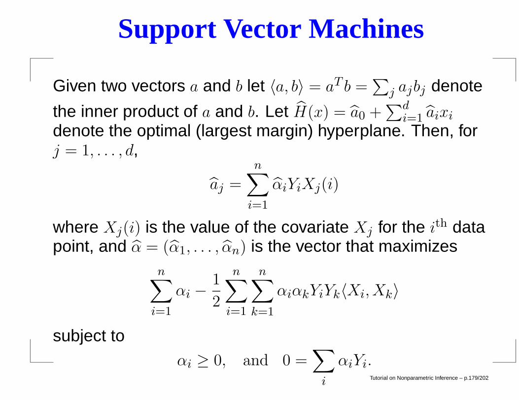
Given two vectors a and b let 〈a, b〉 = aT b =∑
j ajbj denote
the inner product of a and b. Let H(x) = a0 +∑d
i=1 aixidenote the optimal (largest margin) hyperplane. Then, forj = 1, . . . , d,
aj =n∑
i=1
αiYiXj(i)
where Xj(i) is the value of the covariate Xj for the ith datapoint, and α = (α1, . . . , αn) is the vector that maximizes
n∑
i=1
αi −1
2
n∑
i=1
n∑
k=1
αiαkYiYk〈Xi, Xk〉
subject toαi ≥ 0, and 0 =
∑
i
αiYi.Tutorial on Nonparametric Inference – p.179/202
Support Vector Machines
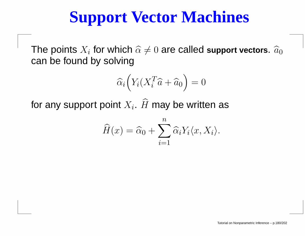
The points Xi for which α 6= 0 are called support vectors. a0
can be found by solving
αi
(Yi(X
Ti a+ a0
)= 0
for any support point Xi. H may be written as
H(x) = α0 +n∑
i=1
αiYi〈x,Xi〉.
Tutorial on Nonparametric Inference – p.180/202
Support Vector Machines
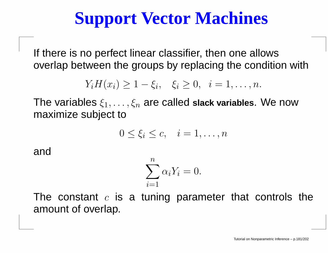
If there is no perfect linear classifier, then one allowsoverlap between the groups by replacing the condition with
YiH(xi) ≥ 1− ξi, ξi ≥ 0, i = 1, . . . , n.
The variables ξ1, . . . , ξn are called slack variables. We nowmaximize subject to
0 ≤ ξi ≤ c, i = 1, . . . , n
andn∑
i=1
αiYi = 0.
The constant c is a tuning parameter that controls theamount of overlap.
Tutorial on Nonparametric Inference – p.181/202
Support Vector Machines
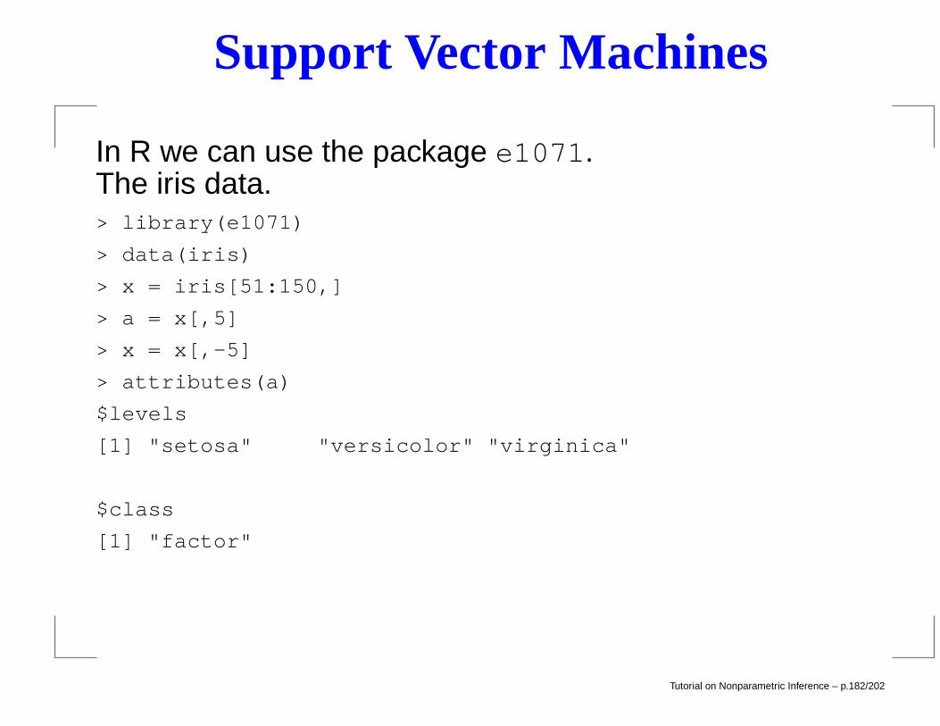
In R we can use the package e1071.The iris data.> library(e1071)
> data(iris)
> x = iris[51:150,]
> a = x[,5]
> x = x[,-5]
> attributes(a)
$levels
[1] "setosa" "versicolor" "virginica"
$class
[1] "factor"
Tutorial on Nonparametric Inference – p.182/202
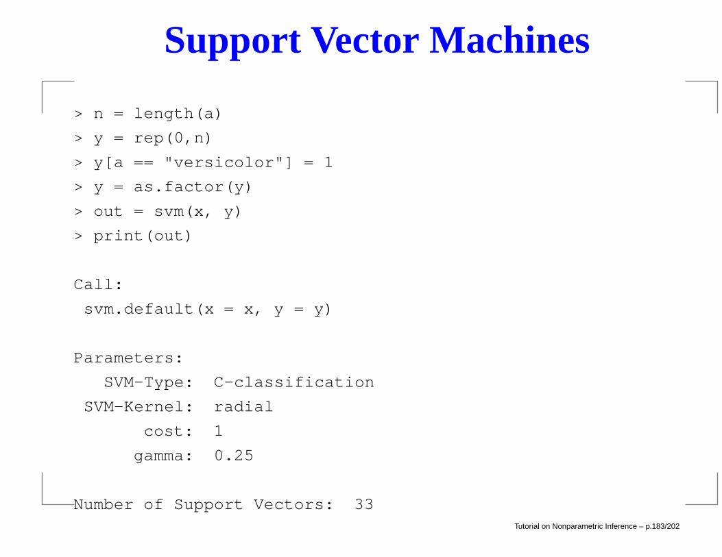
Support Vector Machines
> n = length(a)
> y = rep(0,n)
> y[a == "versicolor"] = 1
> y = as.factor(y)
> out = svm(x, y)
> print(out)
Call:
svm.default(x = x, y = y)
Parameters:
SVM-Type: C-classification
SVM-Kernel: radial
cost: 1
gamma: 0.25
Number of Support Vectors: 33Tutorial on Nonparametric Inference – p.183/202
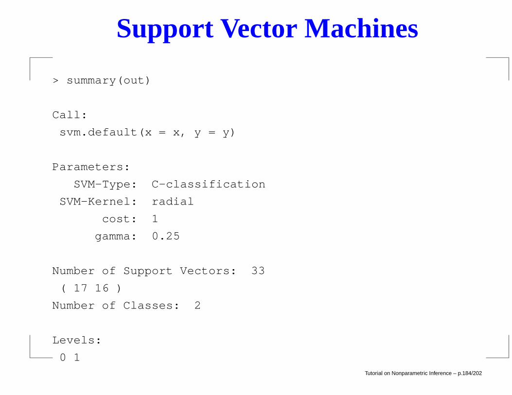
Support Vector Machines
> summary(out)
Call:
svm.default(x = x, y = y)
Parameters:
SVM-Type: C-classification
SVM-Kernel: radial
cost: 1
gamma: 0.25
Number of Support Vectors: 33
( 17 16 )
Number of Classes: 2
Levels:
0 1Tutorial on Nonparametric Inference – p.184/202
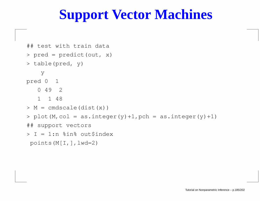
Support Vector Machines
## test with train data
> pred = predict(out, x)
> table(pred, y)
y
pred 0 1
0 49 2
1 1 48
> M = cmdscale(dist(x))
> plot(M,col = as.integer(y)+1,pch = as.integer(y)+1)
## support vectors
> I = 1:n %in% out$index
points(M[I,],lwd=2)
Tutorial on Nonparametric Inference – p.185/202
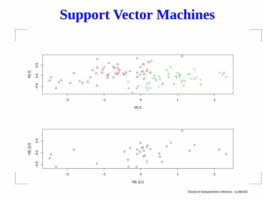
Support Vector Machines
−2 −1 0 1 2
−0.
50.
00.
5
M[,1]
M[,2
]
−2 −1 0 1 2
−0.
50.
00.
5
M[I, ][,1]
M[I,
][,2
]
Tutorial on Nonparametric Inference – p.186/202
Support Vector Machines
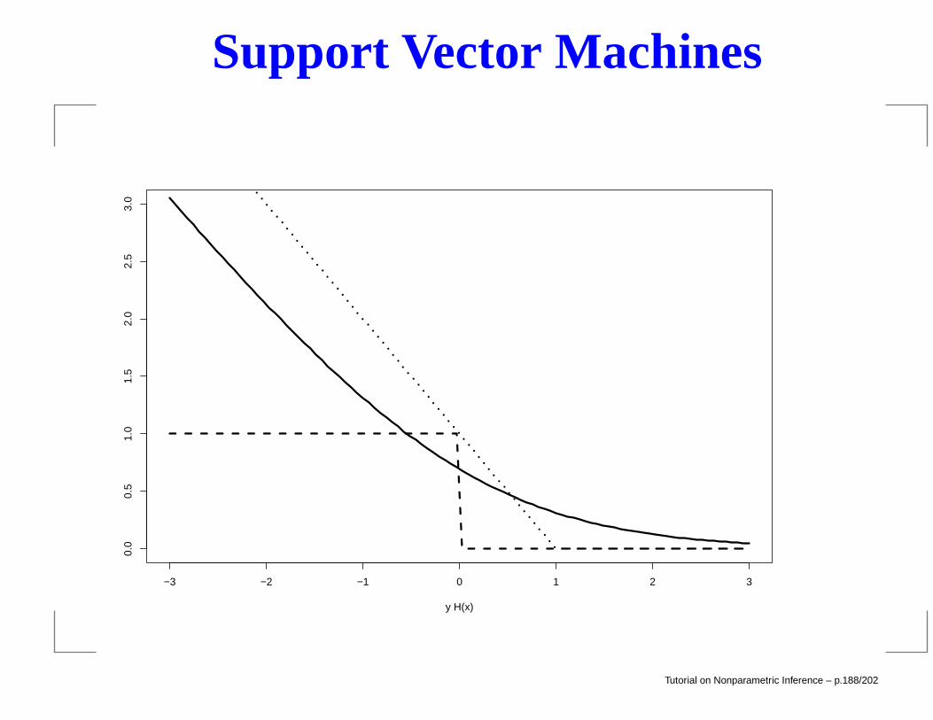
Here is another (easier) way to think about the SVM. TheSVM hyperplan H(x) = β0 + xTx can be obtained byminimizing
n∑
i=1
(1− YiH(Xi))+ + λ||β||2.
The following figure compares the svm loss, squared loss,classification error and logistic loss log(1 + e−yH(x)).
Tutorial on Nonparametric Inference – p.187/202
Support Vector Machines
−3 −2 −1 0 1 2 3
0.0
0.5
1.0
1.5
2.0
2.5
3.0
y H(x)
Tutorial on Nonparametric Inference – p.188/202
Kernelization
There is a trick called kernelization for improving a computa-tionally simple classifier h. The idea is to map the covariateX — which takes values in X — into a higher dimensionalspace Z and apply the classifier in the bigger space Z. Thiscan yield a more flexible classifier while retaining computa-tionally simplicity.
Tutorial on Nonparametric Inference – p.189/202
Kernelization
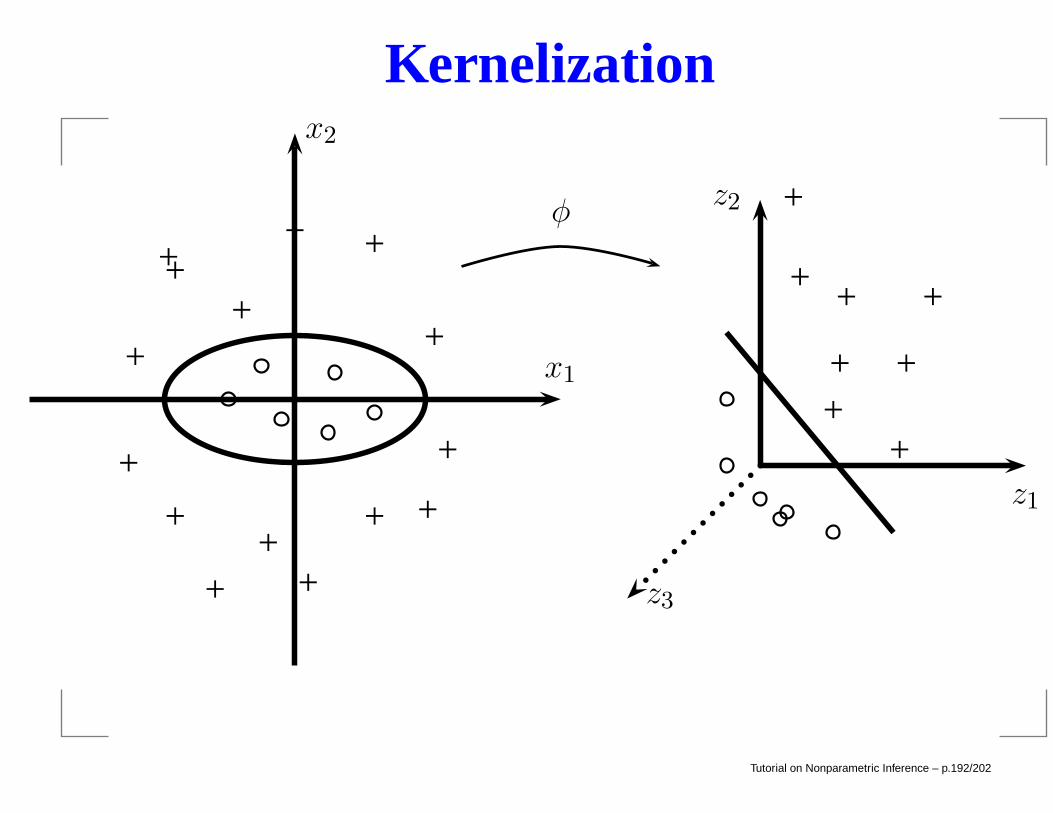
Example: The covariate x = (x1, x2). The Yis can beseparated into two groups using an ellipse. Define amapping φ by
z = (z1, z2, z3) = φ(x) = (x21,√
2x1x2, x22).
Thus, φ maps X = R2 into Z = R
3. In thehigher-dimensional space Z, the Yi’s are separable by alinear decision boundary.
Tutorial on Nonparametric Inference – p.190/202
Kernelization
In other words,
a linear classifier in a higher-dimensional space corresponds to anon-linear classifier in the original space.
The point is that to get a richer set of classifiers we do notneed to give up the convenience of linear classifiers. Wesimply map the covariates to a higher-dimensional space.This is akin to making linear regression more flexible by us-ing polynomials.
Tutorial on Nonparametric Inference – p.191/202
Kernelization
x1
x2
+
+
+
++
+
+ +
+
+
+++
+ +
z1
z2
z3
+
+
++
+
+
+
+
φ
Tutorial on Nonparametric Inference – p.192/202
Kernelization
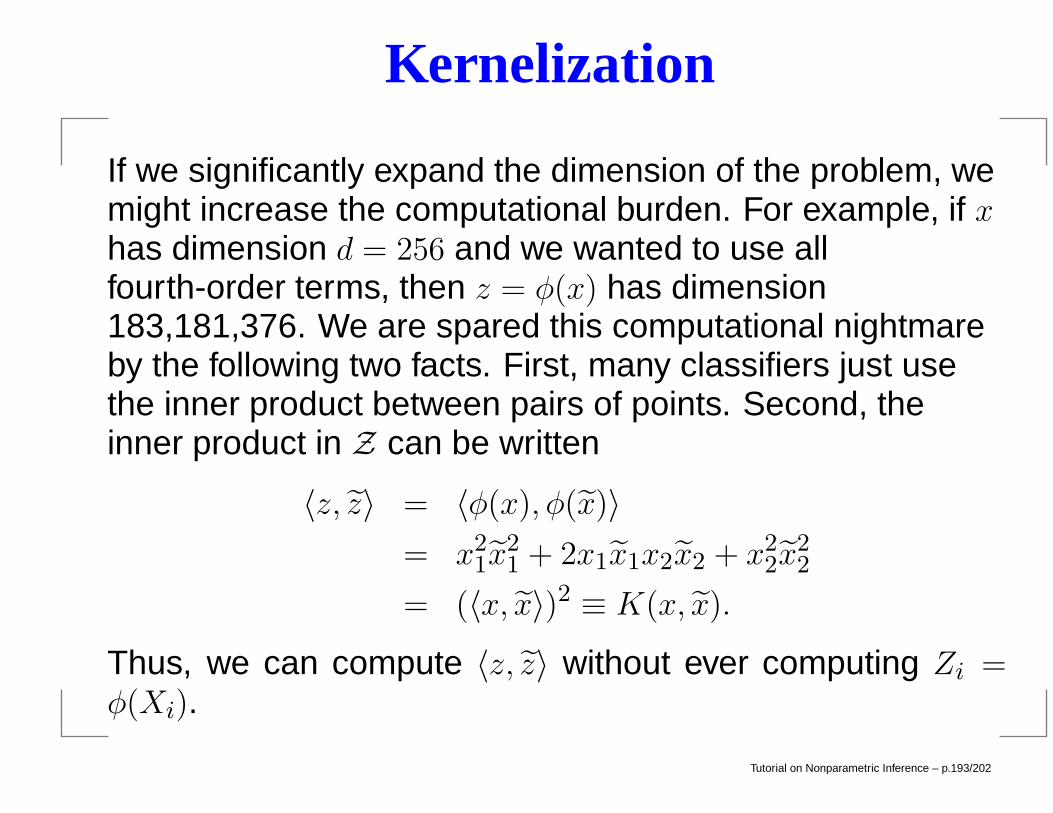
If we significantly expand the dimension of the problem, wemight increase the computational burden. For example, if xhas dimension d = 256 and we wanted to use allfourth-order terms, then z = φ(x) has dimension183,181,376. We are spared this computational nightmareby the following two facts. First, many classifiers just usethe inner product between pairs of points. Second, theinner product in Z can be written
〈z, z〉 = 〈φ(x), φ(x)〉= x2
1x21 + 2x1x1x2x2 + x2
2x22
= (〈x, x〉)2 ≡ K(x, x).
Thus, we can compute 〈z, z〉 without ever computing Zi =φ(Xi).
Tutorial on Nonparametric Inference – p.193/202
Kernelization
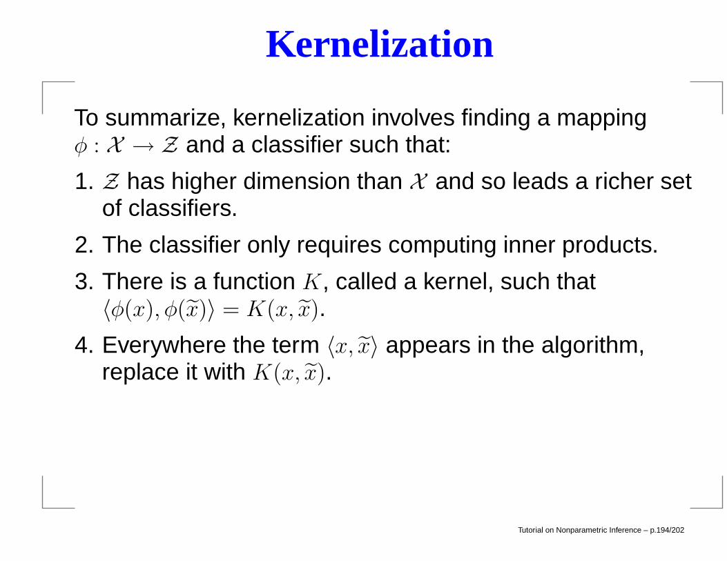
To summarize, kernelization involves finding a mappingφ : X → Z and a classifier such that:
1. Z has higher dimension than X and so leads a richer setof classifiers.
2. The classifier only requires computing inner products.
3. There is a function K, called a kernel, such that〈φ(x), φ(x)〉 = K(x, x).
4. Everywhere the term 〈x, x〉 appears in the algorithm,replace it with K(x, x).
Tutorial on Nonparametric Inference – p.194/202
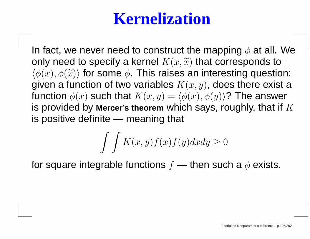
Kernelization
In fact, we never need to construct the mapping φ at all. Weonly need to specify a kernel K(x, x) that corresponds to〈φ(x), φ(x)〉 for some φ. This raises an interesting question:given a function of two variables K(x, y), does there exist afunction φ(x) such that K(x, y) = 〈φ(x), φ(y)〉? The answeris provided by Mercer’s theorem which says, roughly, that if Kis positive definite — meaning that
∫ ∫K(x, y)f(x)f(y)dxdy ≥ 0
for square integrable functions f — then such a φ exists.
Tutorial on Nonparametric Inference – p.195/202
Kernelization
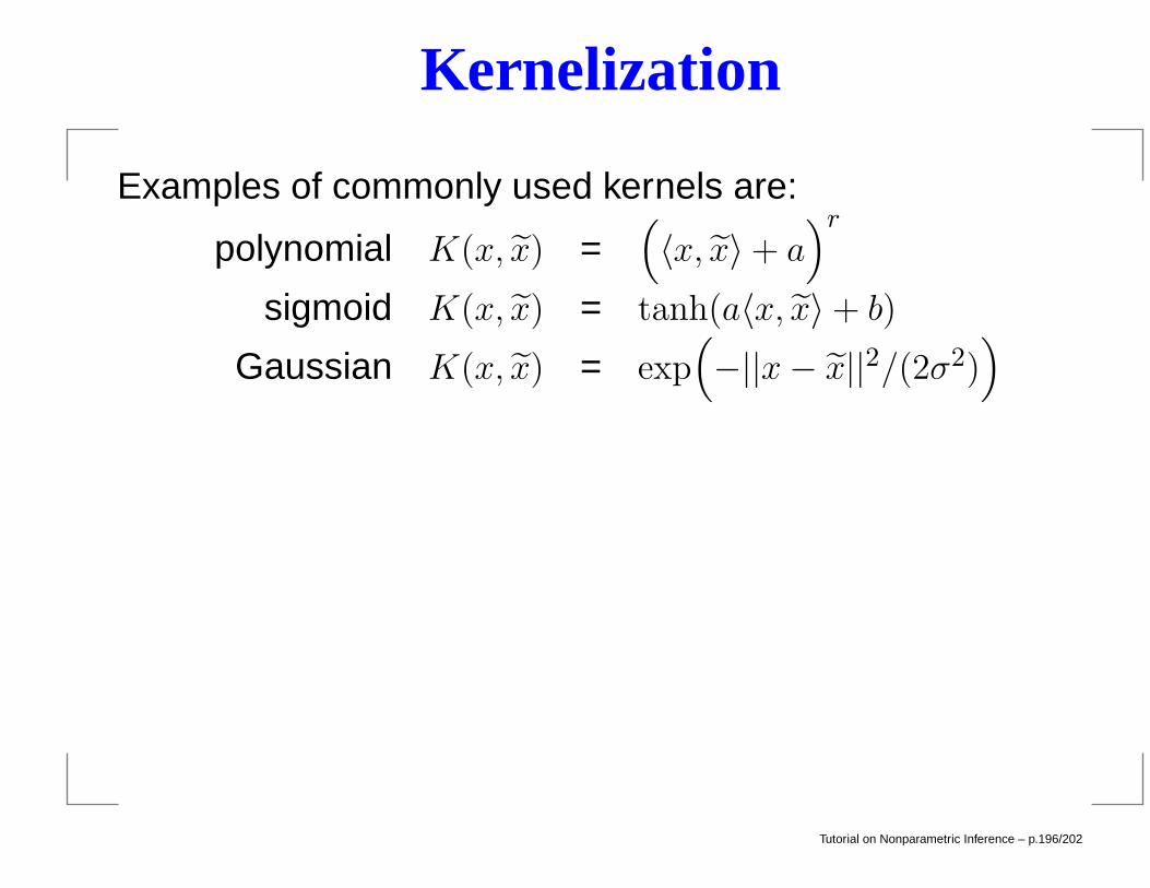
Examples of commonly used kernels are:
polynomial K(x, x) =(〈x, x〉+ a
)r
sigmoid K(x, x) = tanh(a〈x, x〉+ b)
Gaussian K(x, x) = exp(−||x− x||2/(2σ2)
)
Tutorial on Nonparametric Inference – p.196/202
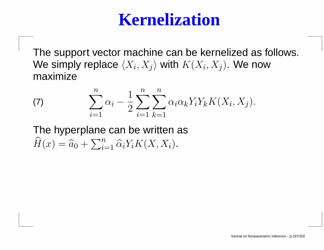
Kernelization
The support vector machine can be kernelized as follows.We simply replace 〈Xi, Xj〉 with K(Xi, Xj). We nowmaximize
n∑
i=1
αi −1
2
n∑
i=1
n∑
k=1
αiαkYiYkK(Xi, Xj).(7)
The hyperplane can be written asH(x) = a0 +
∑ni=1 αiYiK(X,Xi).
Tutorial on Nonparametric Inference – p.197/202
Other Classifiers
1. Bagging
2. Boosting
3. Neural Networks
Tutorial on Nonparametric Inference – p.198/202
A Few Words on Nonparametric Bayes
Nonparametric Bayes is becoming very popular. It isappealing because of (i) conceptual simplicity and (ii) canbe implmented by simulation.Advantages:
1. Easy to understand.
2. Can incorporate prior information.
Disadvantages:
1. Requires specifying an infinite dimensional prior.
2. Not falsifiable (no long run guarantees). In fact, theytypically have near 0 frequency coverage.
Tutorial on Nonparametric Inference – p.199/202
Nonparametric Bayes
Yi = f(Xi) + εi
Assume f lives in some functions space, for example:
f ∈ F =
f :
∫(f ′′(x))2dx <∞
.
Now put a prior π on f . Then get the posterior by Bayes’theorem:
π(f ∈ A)︸ ︷︷ ︸prior
data D−→ π(f ∈ A|D)︸ ︷︷ ︸posterior
Can now find Bayesian confidence bands (L,U):
P(L(x) ≤ f(x) ≤ U(x)|D) = 1− α.
Tutorial on Nonparametric Inference – p.200/202
But ...
How often will (L,U) tarp f in the frequency sense? In otherwords, what is:
Pf (L(x) ≤ f(x) ≤ U(x))??
Answer: typically,
Pf (L(x) ≤ f(x) ≤ U(x)) ≈ 0.
Why? The prior adds bias which causes the bands to becentered away from the true f . That’s why choosingsmoothing parameters is so hard!
Tutorial on Nonparametric Inference – p.201/202
Some References
Diaconis and Freedman (1986)
Shen and Wasserman (2001)
Ghosal, Ghosh and van der Vaart (2000)
Zhao (2000)
Freedman (1963)
Cox (1993)
Tutorial on Nonparametric Inference – p.202/202