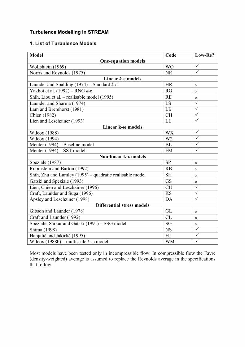
Turbulence Modelling in STREAM 1. List of Turbulence Models

Model Code Low-Re?

One-equation models

Wolfshtein (1969) WO

Norris and Reynolds (1975) NR

Linear k-ε models

Launder and Spalding (1974) – Standard k-ε HR

Yakhot et al. (1992) – RNG k-ε RG

Shih, Liou et al. – realisable model (1995) RE

Launder and Sharma (1974) LS

Lam and Bremhorst (1981) LB

Chien (1982) CH

Lien and Leschziner (1993) LL

Linear k-ω models

Wilcox (1988) WX

Wilcox (1994) W2

Menter (1994) – Baseline model BL

Menter (1994) – SST model FM

Non-linear k-ε models

Speziale (1987) SP

Rubinstein and Barton (1992) RB

Shih, Zhu and Lumley (1995) – quadratic realisable model SH

Gatski and Speziale (1993) GS

Lien, Chien and Leschziner (1996) CU

Craft, Launder and Suga (1996) KS

Apsley and Leschziner (1998) DA

Differential stress models

Gibson and Launder (1978) GL

Craft and Launder (1992) CL

Speziale, Sarkar and Gatski (1991) – SSG model SG

Shima (1998) NS

Hanjalić and Jakirlić (1995) HJ

Wilcox (1988b) – multiscale k-ω model WM

Most models have been tested only in incompressible flow. In compressible flow the Favre

(density-weighted) average is assumed to replace the Reynolds average in the specifications

that follow.

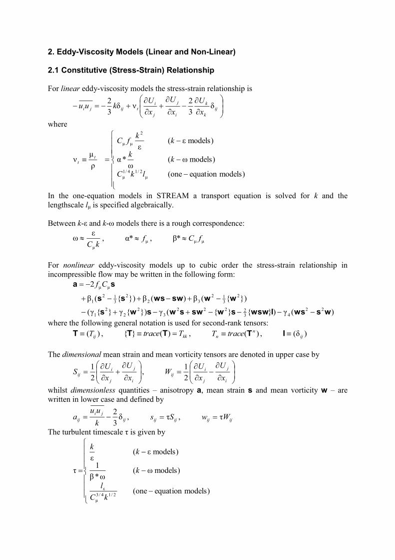
2. Eddy-Viscosity Models (Linear and Non-Linear) 2.1 Constitutive (Stress-Strain) Relationship

For linear eddy-viscosity models the stress-strain relationship is

ij

k

k

i

j

j

i

tijjix

U

x

U

x

Ukuu δ

3

2νδ

3

2

where

)modelsequationone(

)modelsω(ω

*α

)modelsε(ε

ρ

μν

μ

2/14/1

μ

2

μμ

lkC

kk

kk

fC

t

t

In the one-equation models in STREAM a transport equation is solved for k and the

lengthscale lμ is specified algebraically.

Between k-ε and k-ω models there is a rough correspondence:

kCμ

εω , μ*α f , μμ*β fC

For nonlinear eddy-viscosity models up to cubic order the stress-strain relationship in

incompressible flow may be written in the following form:

)(γ)}{}{(γ}){γ}{γ(

}){(β)(β}){(β

2

22

432222

3

2

2

2

1

2

312

32

2

312

1

μμ

wswsIwswswswswsws

wwswwsss

sa

Cf

where the following general notation is used for second-rank tensors:

)( ijTT , kkTtrace )(}{ TT , )( n

n traceT T , )δ( ijI

The dimensional mean strain and mean vorticity tensors are denoted in upper case by

i

j

j

i

ijx

U

x

US

2

1,

i

j

j

i

ijx

U

x

UW

2

1

whilst dimensionless quantities – anisotropy a, mean strain s and mean vorticity w – are

written in lower case and defined by

ij

ji

ijk

uua δ

3

2 , ijij Ss τ , ijij Ww τ

The turbulent timescale τ is given by

)modelsequationone(

)modelsω(ω*β

1

)modelsε(ε

τ

2/14/3

μ

ε

kC

l

k

kk

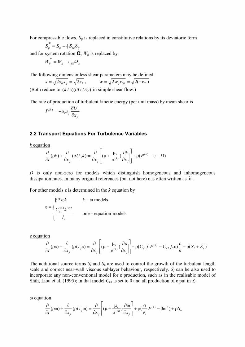
For compressible flows, Sij is replaced in constitutive relations by its deviatoric form

ijkkijij SSS δ*31

and for system rotation Ω, Wij is replaced by

kijkijij WW Ωε*

The following dimensionless shear parameters may be defined:

222 ssss ijij , )(22 2wwww ijij

(Both reduce to )/)(ε/( yUk in simple shear flow.)

The rate of production of turbulent kinetic energy (per unit mass) by mean shear is

j

i

ji

k

x

UuuP

)(

2.2 Transport Equations For Turbulence Variables

k equation

)ε(ρ)σ

μμ()ρ()ρ( )(

)(DP

x

k

xkU

xk

t

k

j

k

t

j

j

j

D is only non-zero for models which distinguish homogeneous and inhomogeneous

dissipation rates. In many original references (but not here) ε is often written as ε~ .

For other models ε is determined in the k equation by

modelsequationone

modelsωω*β

ε

ε

2/34/3

μ

l

kC

kk

ε equation

)(ρε

)ε(ρε

)σ

μμ()ερ()ρε( ε22ε

)(

11ε)ε(SS

kfCPfC

xxU

xtl

k

j

t

j

j

j

The additional source terms Sl and Sε are used to control the growth of the turbulent length

scale and correct near-wall viscous sublayer behaviour, respectively. Sl can be also used to

incorporate any non-conventional model for ε production, such as in the realisable model of

Shih, Liou et al. (1995); in that model Cε1 is set to 0 and all production of ε put in Sl.

ω equation

ω

2)(

)ω(ρ)βω

ν

α(ρ

ω)

σ

μμ()ωρ()ρω( SP

xxU

xt

k

tj

t

j

j

j

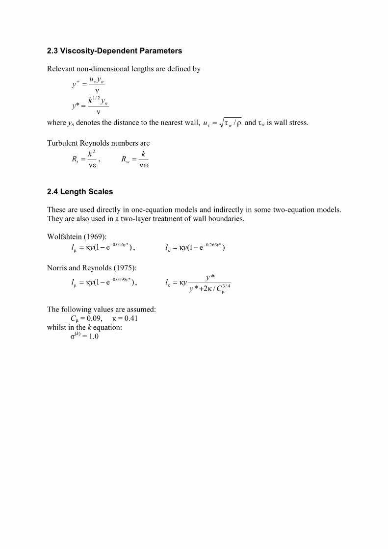
2.3 Viscosity-Dependent Parameters

Relevant non-dimensional lengths are defined by

ν

τ nyuy

ν

*2/1

nyky

where yn denotes the distance to the nearest wall, ρ/ττ wu and τw is wall stress.

Turbulent Reynolds numbers are

νε

2kRt ,

νω

kRw

2.4 Length Scales

These are used directly in one-equation models and indirectly in some two-equation models.

They are also used in a two-layer treatment of wall boundaries.

Wolfshtein (1969):

)e1(κ *016.0

μ

yyl , )e1(κ *263.0

ε

yyl

Norris and Reynolds (1975):

)e1(κ *0198.0

μ

yyl , 4/3

μ

ε/κ2*

*κ

Cy

yyl

The following values are assumed:

Cμ = 0.09, κ = 0.41

whilst in the k equation:

σ(k)

= 1.0

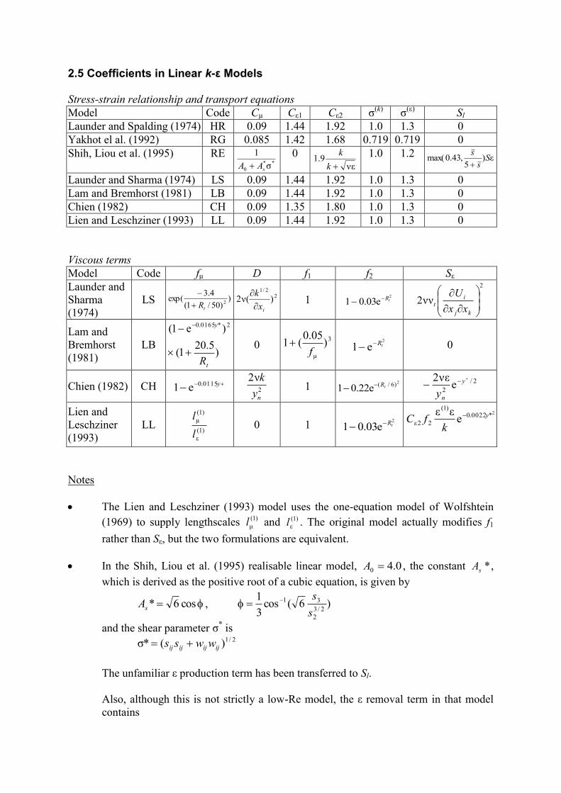
2.5 Coefficients in Linear k-ε Models

Stress-strain relationship and transport equations

Model Code Cμ Cε1 Cε2 σ(k)

σ(ε)

Sl

Launder and Spalding (1974) HR 0.09 1.44 1.92 1.0 1.3 0

Yakhot el al. (1992) RG 0.085 1.42 1.68 0.719 0.719 0

Shih, Liou et al. (1995) RE **

0 σ

1

sAA 0

νε9.1

k

k 1.0 1.2 ε)5

,43.0max( Ss

s

Launder and Sharma (1974) LS 0.09 1.44 1.92 1.0 1.3 0

Lam and Bremhorst (1981) LB 0.09 1.44 1.92 1.0 1.3 0

Chien (1982) CH 0.09 1.35 1.80 1.0 1.3 0

Lien and Leschziner (1993) LL 0.09 1.44 1.92 1.0 1.3 0

Viscous terms

Model Code fμ D f1 f2 Sε

Launder and

Sharma

(1974)

LS ))50/1(

4.3exp(

2

tR

22/1

)(ν2ix

k

1 2

e03.01 tR

2

νν2

kj

i

txx

U

Lam and

Bremhorst

(1981)

LB )

5.201(

)e1( 2*0165.0

t

y

R

0 3

μ

)05.0

(1f

2

e1 tR 0

Chien (1982) CH y0115.0e1 2

ν2

ny

k 1

2)6/(e22.01 tR

2/

2e

νε2 y

ny

Lien and

Leschziner

(1993)

LL )1(

ε

)1(

μ

l

l 0 1

2

e03.01 tR

2*0022.0)1(

22ε eεε y

kfC

Notes

The Lien and Leschziner (1993) model uses the one-equation model of Wolfshtein

(1969) to supply lengthscales )1(

μl and )1(

εl . The original model actually modifies f1

rather than Sε, but the two formulations are equivalent.

In the Shih, Liou et al. (1995) realisable linear model, 0.40 A , the constant *sA ,

which is derived as the positive root of a cubic equation, is given by

cos6*sA , )6(cos3

12/3

2

31

s

s

and the shear parameter σ* is

2/1)(*σ ijijijij wwss

The unfamiliar ε production term has been transferred to Sl.

Also, although this is not strictly a low-Re model, the ε removal term in that model

contains

νε

ε 2

k

rather than the more common ε2/k. This is implemented in the common form by

setting Cε2 as given in the table.

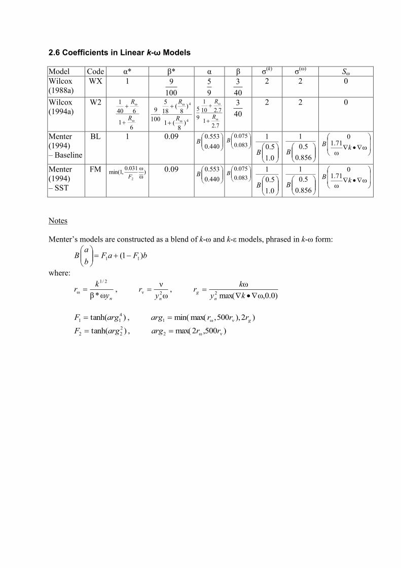
2.6 Coefficients in Linear k-ω Models

Model Code α* β* α β σ(k)

σ(ω)

Sω

Wilcox

(1988a)

WX 1

100

9

9

5

40

3

2 2 0

Wilcox

(1994a)

W2

61

640

1

ω

ω

R

R

4ω

4ω

)8

(1

)8

(18

5

100

9

R

R

7.21

7.210

1

9

5

ω

ω

R

R

40

3

2 2 0

Menter

(1994)

– Baseline

BL 1 0.09

440.0

553.0B

083.0

075.0B

0.1

5.0

1

B

856.0

5.0

1

B

ωω

71.10

kB

Menter

(1994)

– SST

FM )ω

ω031.0,1min(

2F

0.09

440.0

553.0B

083.0

075.0B

0.1

5.0

1

B

856.0

5.0

1

B

ωω

71.10

kB

Notes

Menter’s models are constructed as a blend of k-ω and k-ε models, phrased in k-ω form:

bFaFb

aB )1( 11

where:

ny

kr

ω*β

2/1

ω , ω

ν2ν

nyr ,

)0.0,ωmax(

ω2

ky

kr

n

g

)tanh( 4

11 argF , )2),500,max(min( νω1 grrrarg

)tanh( 2

22 argF , )500,2max( νω2 rrarg

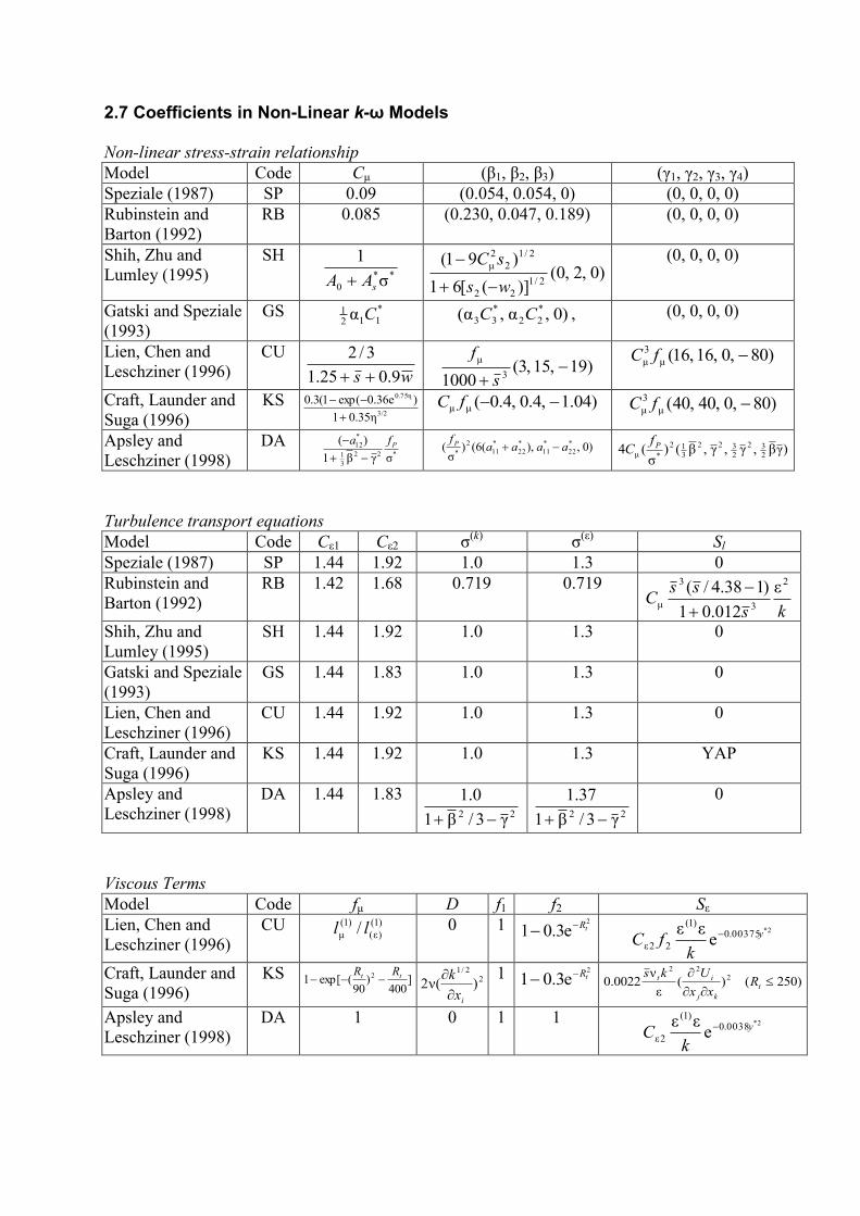
2.7 Coefficients in Non-Linear k-ω Models

Non-linear stress-strain relationship

Model Code Cμ (β1, β2, β3) (γ1, γ2, γ3, γ4)

Speziale (1987) SP 0.09 (0.054, 0.054, 0) (0, 0, 0, 0)

Rubinstein and

Barton (1992)

RB 0.085 (0.230, 0.047, 0.189) (0, 0, 0, 0)

Shih, Zhu and

Lumley (1995)

SH **

0 σ

1

sAA )0,2,0(

)]([61

)91(

2/1

22

2/1

2

2

μ

ws

sC

(0, 0, 0, 0)

Gatski and Speziale

(1993)

GS *

1121 α C )0,α,α( *

22

*

33 CC , (0, 0, 0, 0)

Lien, Chen and

Leschziner (1996)

CU

ws 9.025.1

3/2

)19,15,3(

1000 3

μ

s

f

)80,0,16,16(μ

3

μ fC

Craft, Launder and

Suga (1996)

KS 3/2

η75.0

η0.351

)e36.0exp(1(3.0

)04.1,4.0,4.0(μμ fC )80,0,40,40(μ

3

μ fC

Apsley and

Leschziner (1998)

DA *22

3

1

*

12

σγβ1

)( Pfa

)0,),(6()σ

( *

22

*

11

*

22

*

11

2

*aaaa

f P )γβ,γ,γ,β()

σ(4

232

2322

312

*μPf

C

Turbulence transport equations

Model Code Cε1 Cε2 σ(k)

σ(ε)

Sl

Speziale (1987) SP 1.44 1.92 1.0 1.3 0

Rubinstein and

Barton (1992)

RB 1.42 1.68 0.719 0.719

ks

ssC

2

3

3

μ

ε

012.01

)138.4/(

Shih, Zhu and

Lumley (1995)

SH 1.44 1.92 1.0 1.3 0

Gatski and Speziale

(1993)

GS 1.44 1.83 1.0 1.3 0

Lien, Chen and

Leschziner (1996)

CU 1.44 1.92 1.0 1.3 0

Craft, Launder and

Suga (1996)

KS 1.44 1.92 1.0 1.3 YAP

Apsley and

Leschziner (1998)

DA 1.44 1.83 22 γ3/β1

0.1

22 γ3/β1

37.1

0

Viscous Terms

Model Code fμ D f1 f2 Sε

Lien, Chen and

Leschziner (1996)

CU )1(

)ε(

)1(

μ / ll 0 1 2

e3.01 tR 2*00375.0

)1(

22ε eεε y

kfC

Craft, Launder and

Suga (1996)

KS ]400

)90

(exp[1 2 tt RR 2

2/1

)(ν2ix

k

1 2

e3.01 tR )250()(

ε

ν0022.0 2

22

t

kj

it Rxx

Uks

Apsley and

Leschziner (1998)

DA 1 0 1 1 2*0038.0)1(

2ε eεε y

kC

Notes

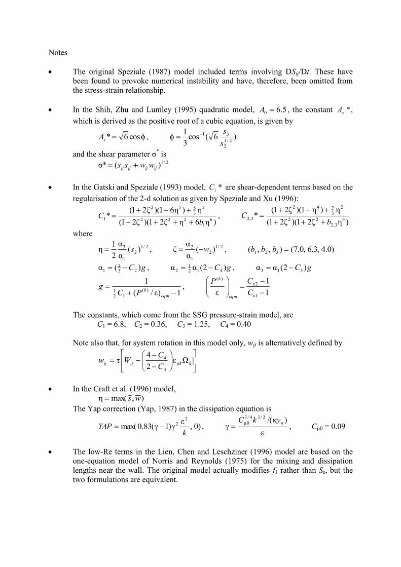
The original Speziale (1987) model included terms involving DSij/Dt. These have

been found to provoke numerical instability and have, therefore, been omitted from

the stress-strain relationship.

In the Shih, Zhu and Lumley (1995) quadratic model, 5.60 A , the constant *sA ,

which is derived as the positive root of a cubic equation, is given by

cos6*sA , )6(cos3

12/3

2

31

s

s

and the shear parameter σ* is

2/1)(*σ ijijijij wwss

In the Gatski and Speziale (1993) model, *iC are shear-dependent terms based on the

regularisation of the 2-d solution as given by Speziale and Xu (1996):

)η6ηζ21)(ζ21(

η)η61)(ζ21(*

6

1

222

2

3552

1b

C

,

)ηζ21)(ζ21(

η)η1)(ζ21(*

6

3,2

22

2

3242

3,2b

C

where

2/1

2

1

3 )(α

α

2

1η s ,

2/1

2

1

2 )(α

αζ w , )0.4,3.6,0.7(),,( 321 bbb

gC )(α 234

1 , gC )2(αα 4121

2 , gC )2(αα 313

1)ε/(

1)(

121

eqm

kPCg ,

1

1

ε 1ε

2ε

)(

C

CP

eqm

k

The constants, which come from the SSG pressure-strain model, are

C1 = 6.8, C2 = 0.36, C3 = 1.25, C4 = 0.40

Note also that, for system rotation in this model only, wij is alternatively defined by

kijkijij

C

CWw Ωε

2

4τ

4

4

In the Craft et al. (1996) model,

),max(η ws

The Yap correction (Yap, 1987) in the dissipation equation is

)0,ε

γ)1γ(83.0max(2

2

kYAP ,

ε

)κ/(γ

2/34/3

0μ nykC , Cμ0 = 0.09

The low-Re terms in the Lien, Chen and Leschziner (1996) model are based on the

one-equation model of Norris and Reynolds (1975) for the mixing and dissipation

lengths near the wall. The original model actually modifies f1 rather than Sε, but the

two formulations are equivalent.

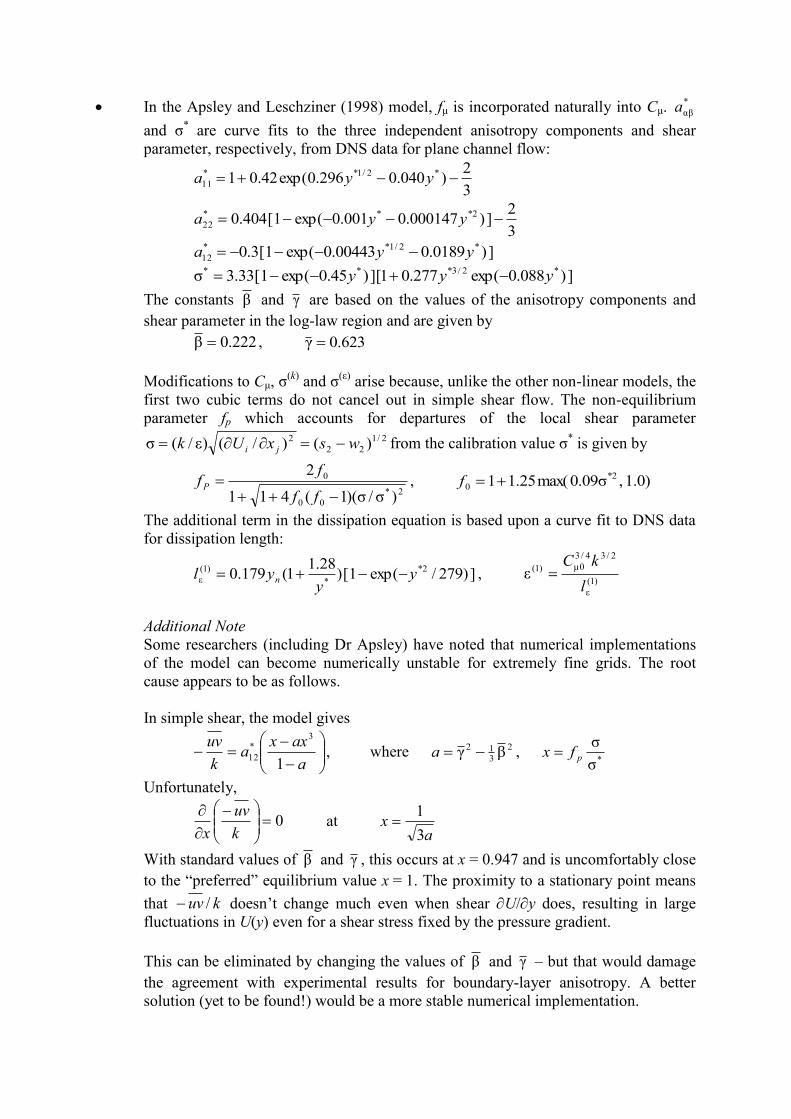
In the Apsley and Leschziner (1998) model, fμ is incorporated naturally into Cμ. *

αβa

and σ* are curve fits to the three independent anisotropy components and shear

parameter, respectively, from DNS data for plane channel flow:

3

2)040.0296.0exp(42.01 *2/1**

11 yya

3

2])000147.0001.0exp(1[404.0 2***

22 yya

])0189.000443.0exp(1[3.0 *2/1**

12 yya

])088.0exp(277.01[])45.0exp(1[33.3σ *2/3*** yyy

The constants β and γ are based on the values of the anisotropy components and

shear parameter in the log-law region and are given by

222.0β , 623.0γ

Modifications to Cμ, σ(k)

and σ(ε)

arise because, unlike the other non-linear models, the

first two cubic terms do not cancel out in simple shear flow. The non-equilibrium

parameter fp which accounts for departures of the local shear parameter 2/1

22

2 )()/()ε/(σ wsxUk ji from the calibration value σ* is given by

2*

00

0

)σ/σ)(1(411

2

ff

ff P , )0.1,σ09.0max(25.11 2*

0 f

The additional term in the dissipation equation is based upon a curve fit to DNS data

for dissipation length:

])279/exp(1[)28.1

1(179.0 2*

*

)1(

ε yy

yl n , )1(

ε

2/34/3

0μ)1(εl

kC

Additional Note

Some researchers (including Dr Apsley) have noted that numerical implementations

of the model can become numerically unstable for extremely fine grids. The root

cause appears to be as follows.

In simple shear, the model gives

a

axxa

k

uv

1

3*

12 , where 2

312 βγ a ,

*σ

σpfx

Unfortunately,

0

k

uv

x at

ax

3

1

With standard values of β and γ , this occurs at x = 0.947 and is uncomfortably close

to the “preferred” equilibrium value x = 1. The proximity to a stationary point means

that kuv / doesn’t change much even when shear U/y does, resulting in large

fluctuations in U(y) even for a shear stress fixed by the pressure gradient.

This can be eliminated by changing the values of β and γ – but that would damage

the agreement with experimental results for boundary-layer anisotropy. A better

solution (yet to be found!) would be a more stable numerical implementation.

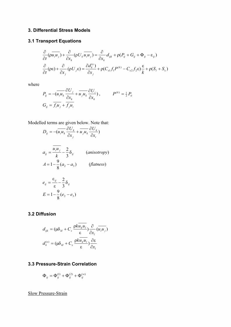
3. Differential Stress Models

3.1 Transport Equations

)εΦ(ρ)ρ()ρ( ijijijijijk

k

jik

k

ji GPdx

uuUx

uut

)(ρε

)ε(ρ)

)ερ()ρε( ε22ε

)(

11ε

ε(

SSk

fCPfCx

dU

xtl

k

j

kj

j

where

)(k

i

kj

k

j

kiijx

Uuu

x

UuuP

, ii

k PP21)(

ijjiij ufufG

Modelled terms are given below. Note that:

)(i

k

kj

j

k

kiijx

Uuu

x

UuuD

ij

ji

ijk

uua δ

3

2 (anisotropy)

)(8

91 32 aaA (flatness)

ij

ij

ije δ3

2

ε

ε

)(8

91 32 eeE

3.2 Diffusion

)()ε

ρμδ( ji

l

lksklijk uu

x

uukCd

l

lkklk

x

uukCd

ε)

ε

ρμδ( ε

)ε(

3.3 Pressure-Strain Correlation

)()2()1( ΦΦΦΦ w

ijijijij

Slow Pressure-Strain

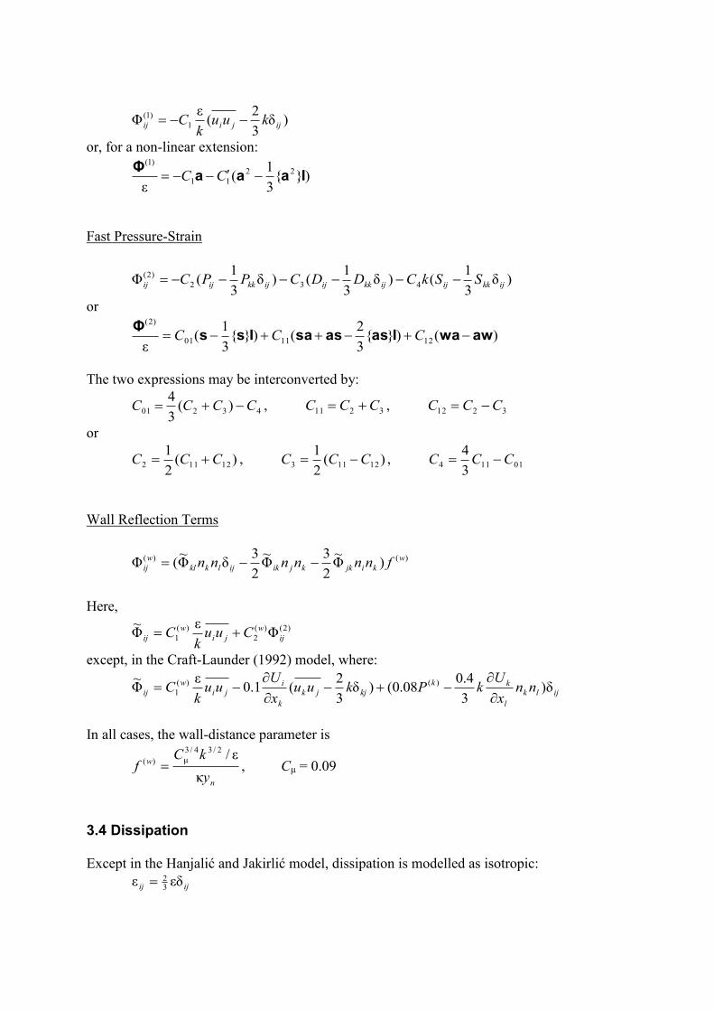
)δ3

2(

εΦ 1

)1(

ijjiij kuuk

C

or, for a non-linear extension:

)}{3

1(

ε

22

11

)1(

IaaaΦ

CC

Fast Pressure-Strain

)δ3

1()δ

3

1()δ

3

1(Φ 432

)2(

ijkkijijkkijijkkijij SSkCDDCPPC

or

)()}{3

2()}{

3

1(

ε121101

)2(

awwaIasassaIssΦ

CCC

The two expressions may be interconverted by:

43201 )(3

4CCCC , 3211 CCC , 3212 CCC

or

)(2

112112 CCC , )(

2

112113 CCC , 01114

3

4CCC

Wall Reflection Terms

)()( )Φ~

2

3Φ~

2

3δΦ

~(Φ w

kijkkjikijlkkl

w

ij fnnnnnn

Here,

)2()(

2

)(

1 Φε

Φ~

ij

w

ji

w

ij Cuuk

C

except, in the Craft-Launder (1992) model, where:

ijlk

l

kk

kjjk

k

i

ji

w

ij nnx

UkPkuu

x

Uuu

kC δ)

3

4.008.0()δ

3

2(1.0

εΦ~ )()(

1

In all cases, the wall-distance parameter is

n

w

y

kCf

κ

ε/2/34/3

μ)( , Cμ = 0.09

3.4 Dissipation

Except in the Hanjalić and Jakirlić model, dissipation is modelled as isotropic:

ijij εδε32

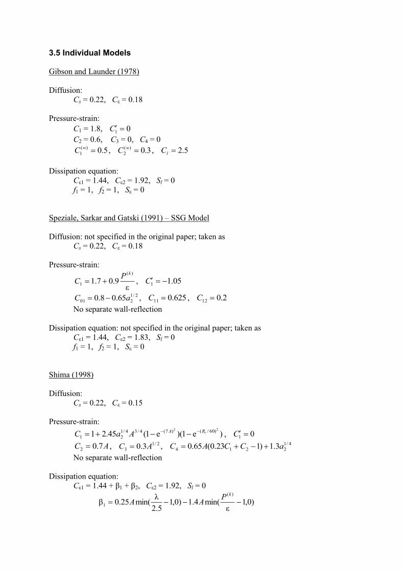
3.5 Individual Models

Gibson and Launder (1978)

Diffusion:

Cs = 0.22, Cε = 0.18

Pressure-strain:

C1 = 1.8, 01 C

C2 = 0.6, C3 = 0, C4 = 0

5.0)(

1 wC , 3.0)(

2 wC , 5.2lC

Dissipation equation:

Cε1 = 1.44, Cε2 = 1.92, Sl = 0

f1 = 1, f2 = 1, Sε = 0

Speziale, Sarkar and Gatski (1991) – SSG Model

Diffusion: not specified in the original paper; taken as

Cs = 0.22, Cε = 0.18

Pressure-strain:

ε

9.07.1)(

1

kPC , 05.11 C

2/1

201 65.08.0 aC , 625.011 C , 2.012 C

No separate wall-reflection

Dissipation equation: not specified in the original paper; taken as

Cε1 = 1.44, Cε2 = 1.83, Sl = 0

f1 = 1, f2 = 1, Sε = 0

Shima (1998)

Diffusion:

Cs = 0.22, Cε = 0.15

Pressure-strain:

)e1)(e1(45.2122 )60/()7(4/34/1

21tRAAaC

, 01 C

AC 7.02 , 2/1

3 3.0 AC , 4/1

2214 3.1)123.0(65.0 aCCAC

No separate wall-reflection

Dissipation equation:

Cε1 = 1.44 + β1 + β2, Cε2 = 1.92, Sl = 0

)0,1ε

min(4.1)0,15.2

λmin(25.0β

)(

1 kP

AA

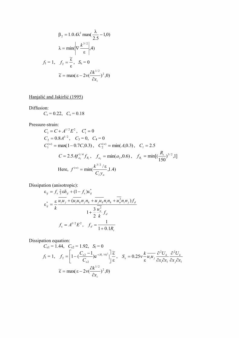
)0,15.2

λmax(λ0.1β 2

2 A

)4,ε

min(λ2/3k

f1 = 1, ε

ε~

2 f , Sε = 0

)0,)(ν2εmax(ε~ 22/1

ix

k

Hanjalić and Jakirlić (1995)

Diffusion:

Cs = 0.22, Cε = 0.18

Pressure-strain:

22/1

1 EACC , 01 C

2/1

2 8.0 AC , C3 = 0, C4 = 0

)3.0,7.01max()(

1 CC w , )3.0,min()(

2 AC w , 5.2lC

tRa fAfC 4/1

25.2 , )6.0,min( 22

afa , ]1,)150

min[( 2/3tR

Rf

t

Here, )4.1,ε/

min(2/3

)(

nl

w

yC

kf

Dissipation (anisotropic):

*

ε32

ε ε)1(εδε ijijij ff

d

n

djinkikjkjkiji

ij

fk

u

fnnunnuunnuuuu

k 2

2

*

2

31

)(εε

22/1

ε EAf , t

dR

f1.01

1

Dissipation equation:

Cε1 = 1.44, Cε2 = 1.92, Sl = 0

f1 = 1, ε

ε~e)

1(1

2)6/(

2ε

2ε

2

tR

C

Cf ,

lj

k

li

kji

xx

U

xx

Uuu

kS

22

εε

ν25.0

)0,)(ν2εmax(ε~ 22/1

ix

k

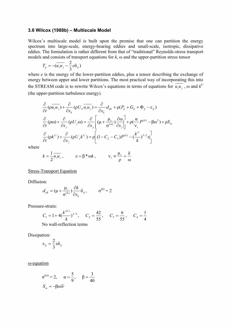
3.6 Wilcox (1988b) – Multiscale Model

Wilcox’s multiscale model is built upon the premise that one can partition the energy

spectrum into large-scale, energy-bearing eddies and small-scale, isotropic, dissipative

eddies. The formulation is rather different from that of “traditional” Reynolds-stress transport

models and consists of transport equations for k, ω and the upper-partition stress tensor

)δ3

2( ijjiij euuT

where e is the energy of the lower-partition eddies, plus a tensor describing the exchange of

energy between upper and lower partitions. The most practical way of incorporating this into

the STREAM code is to rewrite Wilcox’s equations in terms of equations for jiuu , ω and kU

(the upper-partition turbulence energy).

)εΦ(ρ)ρ()ρ( ijijijijijk

k

jik

k

ji GPdx

uuUx

uut

ω

2)(

)ω(ρ)βω

ν

α(ρ

ω)

σ

μμ()ωρ()ρω( SP

xxU

xt

k

tj

t

j

j

j

ε)()1(ρ)ρ()ρ( 2/3)(

32k

kPCCkU

xk

t

UkU

j

j

U

where

iiuuk2

1 , kω*βε ,

ωρ

μν

ktt

Stress-Transport Equation

Diffusion:

ij

k

k

t

ijkx

kd δ)

σ

μμ(

)(

, σ

(k) = 2

Pressure-strain:

2/3)(

1 )(41k

kC

U

, 55

422 C ,

55

63 C ,

4

14 C

No wall-reflection terms

Dissipation:

ijij εδ

3

2ε

ω-equation

σ(ω)

= 2, 9

5α ,

40

3β

wS βωω

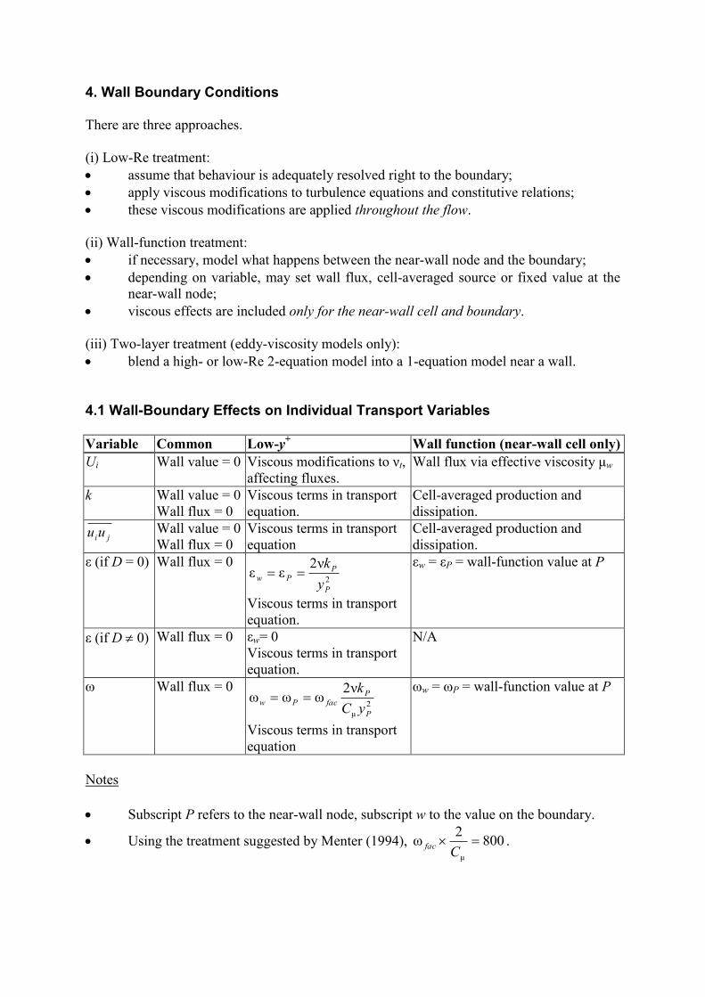
4. Wall Boundary Conditions

There are three approaches.

(i) Low-Re treatment:

assume that behaviour is adequately resolved right to the boundary;

apply viscous modifications to turbulence equations and constitutive relations;

these viscous modifications are applied throughout the flow.

(ii) Wall-function treatment:

if necessary, model what happens between the near-wall node and the boundary;

depending on variable, may set wall flux, cell-averaged source or fixed value at the

near-wall node;

viscous effects are included only for the near-wall cell and boundary.

(iii) Two-layer treatment (eddy-viscosity models only):

blend a high- or low-Re 2-equation model into a 1-equation model near a wall.

4.1 Wall-Boundary Effects on Individual Transport Variables

Variable Common Low-y+ Wall function (near-wall cell only)

Ui Wall value = 0 Viscous modifications to νt,

affecting fluxes.

Wall flux via effective viscosity μw

k Wall value = 0

Wall flux = 0

Viscous terms in transport

equation.

Cell-averaged production and

dissipation.

jiuu Wall value = 0

Wall flux = 0

Viscous terms in transport

equation

Cell-averaged production and

dissipation.

ε (if D = 0) Wall flux = 0 2

ν2εε

P

PPw

y

k

Viscous terms in transport

equation.

εw = εP = wall-function value at P

ε (if D 0) Wall flux = 0 εw= 0

Viscous terms in transport

equation.

N/A

ω Wall flux = 0 2

μ

ν2ωωω

P

PfacPw

yC

k

Viscous terms in transport

equation

ωw = ωP = wall-function value at P

Notes

Subscript P refers to the near-wall node, subscript w to the value on the boundary.

Using the treatment suggested by Menter (1994), 8002

ωμ

C

fac .

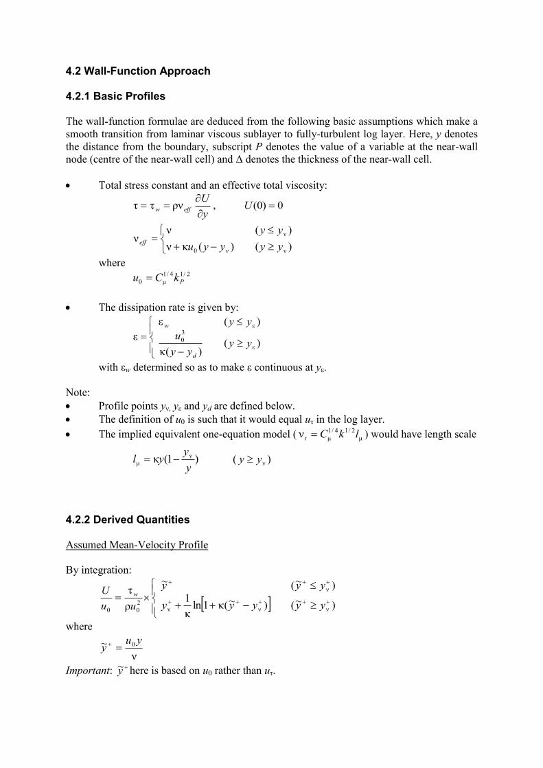
4.2 Wall-Function Approach

4.2.1 Basic Profiles

The wall-function formulae are deduced from the following basic assumptions which make a

smooth transition from laminar viscous sublayer to fully-turbulent log layer. Here, y denotes

the distance from the boundary, subscript P denotes the value of a variable at the near-wall

node (centre of the near-wall cell) and Δ denotes the thickness of the near-wall cell.

Total stress constant and an effective total viscosity:

y

Ueffw

ρνττ , 0)0( U

)()(κν

)(νν

νν0

ν

yyyyu

yyeff

where

2/14/1

μ PkCu

The dissipation rate is given by:

)(

)(κ

)(ε

εε

3

0

ε

yyyy

u

yy

d

w

with εw determined so as to make ε continuous at yε.

Note:

Profile points yν, yε and yd are defined below.

The definition of u0 is such that it would equal uτ in the log layer.

The implied equivalent one-equation model ( μ

2/14/1

μν lkCt ) would have length scale

)1(κ νμ

y

yyl ( νyy )

4.2.2 Derived Quantities

Assumed Mean-Velocity Profile

By integration:

)~()~(κ1lnκ

1

)~(~

ρ

τ

ννν

ν

2

00yyyyy

yyy

uu

U w

where

ν

~ 0 yuy

Important: y~ here is based on u0 rather than uτ.

Wall Stress and Effective Wall Viscosity

P

Pww

y

Uρντ

where

)~(

)~(κ1lnκ

1

~)~(1

ννν

νν

ν

yy

yyy

y

yy

P

P

P

P

w

Cell-Averaged Production and Dissipation

)Δ~

()Δ

~(κ1

)Δ~

(κ)Δ

~(κ1ln

Δκ

)ρ/τ(

)Δ~

(0

ν

ν

ν

ν

0

2

ν

)(

yy

yy

u

y

Pw

k

av

)Δ(

Δln

Δκ

)Δ(ε

εν

ε

ε

ε

3

0

ν

yyy

y

yy

yu

y

dd

d

w

av

Near-Wall Dissipation

εP is given directly from the assumed ε profile at y = yP; i.e.

)(

)(κ

)(ε

εε

3

0

ε

yyyy

u

yy

P

dP

Pw

P

4.2.3 Matching Depths

For smooth walls:

37.7ν y

4.27ε y , 9.4

dy

For arbitrarily-rough walls (Apsley, 2007) the viscous sublayer cutoff is given by:

)κlnκ

1(ν Bfy ,

)0()1(κ

1

)0(

)( κ xe

xx

xf x

and

)ln(κ

1CkBB srough ,

)(κ smoothrough BBeC

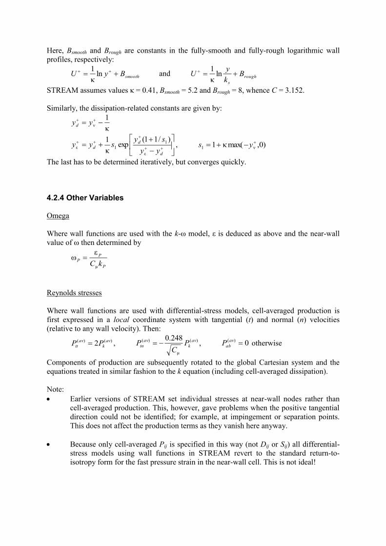
Here, Bsmooth and Brough are constants in the fully-smooth and fully-rough logarithmic wall

profiles, respectively:

smoothByU lnκ

1 and rough

s

Bk

yU ln

κ

1

STREAM assumes values κ = 0.41, Bsmooth = 5.2 and Brough = 8, whence C = 3.152.

Similarly, the dissipation-related constants are given by:

κ

1ν yyd

d

d

dyy

sysyy

ε

1

1ε

)/11(exp

κ

1, )0,max(κ1 ν1

ys

The last has to be determined iteratively, but converges quickly.

4.2.4 Other Variables

Omega

Where wall functions are used with the k-ω model, ε is deduced as above and the near-wall

value of ω then determined by

P

PP

kCμ

εω

Reynolds stresses

Where wall functions are used with differential-stress models, cell-averaged production is

first expressed in a local coordinate system with tangential (t) and normal (n) velocities

(relative to any wall velocity). Then:

)()( 2 av

k

av

tt PP , )(

μ

)( 248.0 av

k

av

tn PC

P , 0)( av

abP otherwise

Components of production are subsequently rotated to the global Cartesian system and the

equations treated in similar fashion to the k equation (including cell-averaged dissipation).

Note:

Earlier versions of STREAM set individual stresses at near-wall nodes rather than

cell-averaged production. This, however, gave problems when the positive tangential

direction could not be identified; for example, at impingement or separation points.

This does not affect the production terms as they vanish here anyway.

Because only cell-averaged Pij is specified in this way (not Dij or Sij) all differential-

stress models using wall functions in STREAM revert to the standard return-to-

isotropy form for the fast pressure strain in the near-wall cell. This is not ideal!

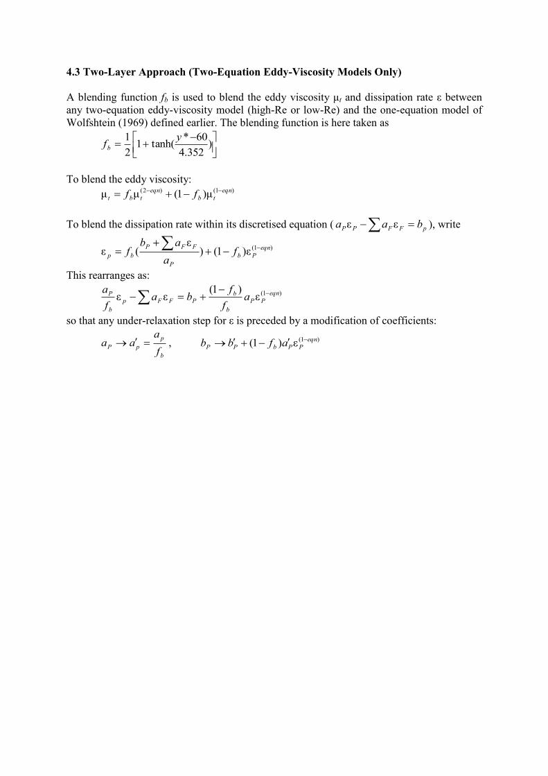
4.3 Two-Layer Approach (Two-Equation Eddy-Viscosity Models Only)

A blending function fb is used to blend the eddy viscosity μt and dissipation rate ε between

any two-equation eddy-viscosity model (high-Re or low-Re) and the one-equation model of

Wolfshtein (1969) defined earlier. The blending function is here taken as

)

352.4

60*tanh(1

2

1 yfb

To blend the eddy viscosity:

)1()2( μ)1(μμ eqn

tb

eqn

tbt ff

To blend the dissipation rate within its discretised equation ( pFFPP baa εε ), write

)1(ε)1()

ε(ε eqn

Pb

P

FFP

bp fa

abf

This rearranges as:

)1(ε

)1(εε eqn

PP

b

b

PFFp

b

P af

fba

f

a

so that any under-relaxation step for ε is preceded by a modification of coefficients:

b

p

pPf

aaa , )1(ε)1( eqn

PPbPP afbb

References

Apsley, D.D., 2007, CFD calculation of turbulent flow with arbitrary wall roughness, Flow,

Turbulence and Combustion, 78, 153-175.

Apsley, D.D. and Leschziner, M.A., 1998, A new low-Reynolds-number nonlinear two-

equation turbulence model for complex flows, Int. J. Heat Fluid Flow, 19, 209-222.

Chien, K.Y., 1982, Predictions of channel and boundary-layer flows with a low-Reynolds-

number turbulence model, AIAA J., 20, 33-38.

Craft, T.J. and Launder, B.E., 1992, New wall-reflection model applied to the turbulent

impinging jet, AIAA J., 30, 2970-2972.

Craft, T.J., Launder, B.E. and Suga, K., 1996, Development and application of a cubic eddy-

viscosity model of turbulence, Int. J. Heat Fluid Flow, 17, 108-115.

Gatski, T.B. and Speziale, C.G., 1993, On explicit algebraic stress models for complex

turbulent flows, J. Fluid Mech., 254, 59-78.

Gibson, M.M. and Launder, B.E., 1978, Ground effects on pressure fluctuations in the

atmospheric boundary layer, J. Fluid Mech., 86, 491-511.

Jakirlić, S. and Hanjalić, K., 1995, A second-moment closure for non-equilibrium and

separating high- and low-Re-number flows, Proc. 10th Symp. Turbulent Shear Flows,

Pennsylvania State University.

Lam, C.K.G. and Bremhorst, K.A., 1981, Modified form of the k-e model for predicting wall

turbulence, Journal of Fluids Engineering, 103, 456-460.

Launder, B.E., Reece, G.J. and Rodi, W., 1975, Progress in the development of a Reynolds-

stress turbulence closure, J. Fluid Mech., 68, 537-566.

Launder, B.E. and Sharma, B.I., 1974, Application of the energy-dissipation model of

turbulence to the calculation of flow near a spinning disc, Letters in Heat and Mass

Transfer, 1, 131-138.

Launder, B.E. and Spalding, D.B., 1974, The numerical computation of turbulent flows,

Computer Meth. Appl. Mech. Eng., 3, 269-289.

Lien, F-S. and Leschziner, M.A., 1993, Second-moment modelling of recirculating flow with

a non-orthogonal collocated finite-volume algorithm, 8th

Symposium on Turbulent

Shear Flows, Munich.

Lien, F.-S., Chen, W.L. and Leschziner, M.A., 1996, Low-Reynolds-number eddy-viscosity

modelling based on non-linear stress-strain/vorticity relations, 3rd

Symp. Engineering

Turbulence Modelling and Measurements, Crete.

Menter, F.R., 1994, Two-equation eddy-viscosity turbulence models for engineering

applications, AIAA J., 32, 1598-1605.

Norris, L.H. and Reynolds, W.C., 1975, Turbulent channel flow with a moving wavy

boundary, Stanford Univ. Dept. Mech. Eng. Rept. FM-10.

Rubinstein, R. and Barton, J.M., 1990, Nonlinear Reynolds stress models and the

renormalisation group, Phys. Fluids A, 2, 1472-1476.

Shih, T.-H., Liou, W.W., Shammir, A., Yang, Z. and Zhu, J., 1995, A new k-ε eddy-viscosity

model for high Reynolds number turbulent flows, Computers Fluids, 24, 227-238.

Shih, T.-H., Zhu, J. and Lumley, J.L., 1995, A new Reynolds stress algebraic equation model,

Comput. Methods Appl. Mech. Engrg., 125, 287-302.

Speziale, C.G., 1987, On nonlinear K-l and K-ε models of turbulence, J. Fluid Mech., 178,

459-475.

Speziale, C.G., Sarkar, S. and Gatski, T.B., 1991, Modelling the pressure-strain correlation of

turbulence: an invariant dynamical systems approach, J. Fluid Mech., 227, 245-272.

Wilcox, D.C., 1988a, Reassessment of the scale-determining equation for advanced

turbulence models, AIAA J., 26, 1299-1310.

Wilcox, D.C., 1988b, Multi-scale model for turbulent flows, AIAA Journal, 26, 1311-1320.

Wilcox, D.C., 1994, Simulation of transition with a two-equation turbulence model, AIAA J.,

32, 247-255.

Wolfshtein, M.W., 1969, The velocity and temperature distribution in one-dimensional flow

with turbulence augmentation and pressure gradient, Int. J. Heat Mass Transfer, 12,

301.

Yakhot, V., Orszag, S.A., Thangam, S., Gatski, T.B. and Speziale, C.G., 1992, Development

of turbulence models for shear flows by a double expansion technique, Phys. Fluids

A, 7, 1510.