Transmission Line Theory - Arraytool · Free Space as a TX LineTX Line Connected to a LoadSome...

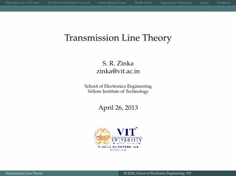
Free Space as a TX Line TX Line Connected to a Load Some Special Cases Smith Chart Impedance Matching Z0&β Problems

Transmission Line Theory

S. R. [email protected]

School of Electronics EngineeringVellore Institute of Technology

April 26, 2013

Transmission Line Theory ECE202, School of Electronics Engineering, VIT

mailto:[email protected]


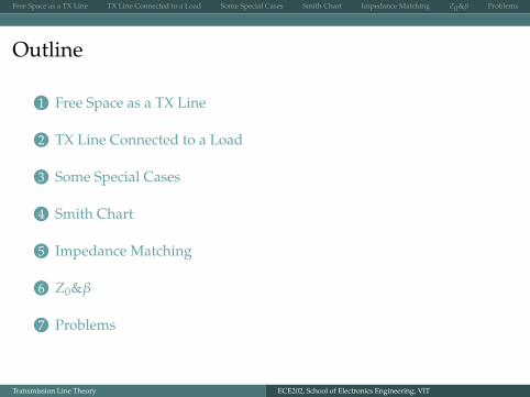
Outline

1 Free Space as a TX Line

2 TX Line Connected to a Load

3 Some Special Cases

4 Smith Chart

5 Impedance Matching

6 Z0&β

7 Problems



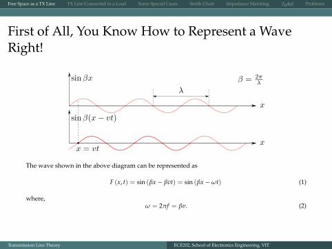
First of All, You Know How to Represent a WaveRight!

The wave shown in the above diagram can be represented as

F (x, t) = sin (βx− βvt) = sin (βx−ωt) (1)

where,ω = 2πf = βv. (2)



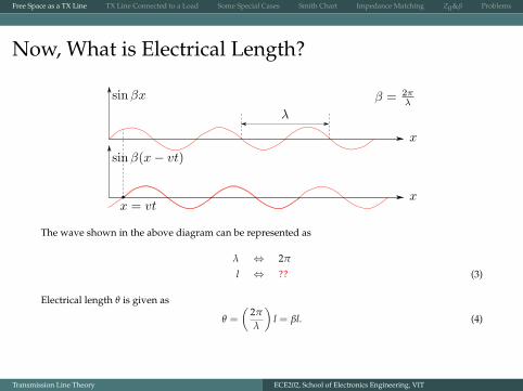
Now, What is Electrical Length?

The wave shown in the above diagram can be represented as

λ ⇔ 2π

l ⇔ ?? (3)

Electrical length θ is given as

θ =

(2π

λ

)l = βl. (4)



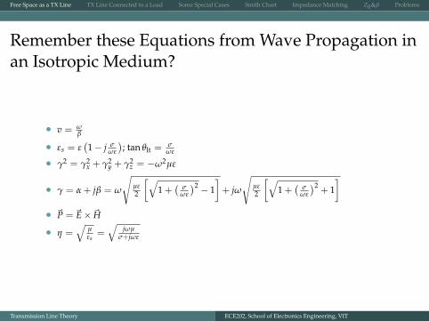
Remember these Equations from Wave Propagation inan Isotropic Medium?

• v = ωβ

• εs = ε(1− j σ

ωε

); tan θlt =

σωε

• γ2 = γ2x + γ2

y + γ2z = −ω2µε

• γ = α + jβ = ω

√µε2

[√1 +

(σ

ωε

)2 − 1]+ jω

√µε2

[√1 +

(σ

ωε

)2+ 1]

• ~P = ~E× ~H

• η =√

µεs

=√

jωµσ+jωε



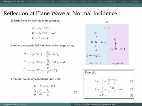
Reflection of Plane Wave at Normal IncidenceElectric fields on both sides are given as,

~Ei = Eie−γz,1zx,

~Et = Ete−γz,1zx, and

~Er = Ereγz,1zx.

Similarly, magnetic fields on both sides are given as,

~Hi = Hie−γz,1zy =

Ei

η1e−γz,1zy,

~Ht = Hte−γz,2zy =Et

η2e−γz,2zy, and

~Hr = Hreγz,1zx = − Er

η1eγz,1zy.

From the boundary conditions (at z = 0),

Ei + Er = Et, and

Ei

η1− Er

η1=

Et

η2. (5)

x

From (5),

Γ =Er

Ei=

η2 − η1

η2 + η1, (6)

τ =Et

Ei=

2η2

η2 + η1, and (7)

1 + Γ = τ. (8)



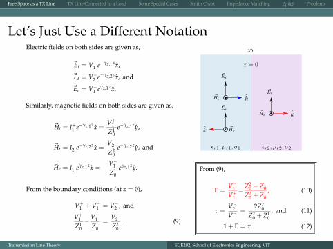
Let’s Just Use a Different NotationElectric fields on both sides are given as,

~Ei = V+1 e−γz,1zx,

~Et = V−2 e−γz,2zx, and

~Er = V−1 eγz,1zx.

Similarly, magnetic fields on both sides are given as,

~Hi = I+1 e−γz,1zx =V+

1

Z10

e−γz,1zy,

~Ht = I−2 e−γz,2zx =V−2Z2

0e−γz,2zy, and

~Hr = I−1 eγz,1zx = −V−1Z1

0eγz,1zy.

From the boundary conditions (at z = 0),

V+1 + V−1 = V−2 , and

V+1

Z10−V−1

Z10

=V−2Z2

0. (9)

x

From (9),

Γ =V−1V+

1=

Z20 − Z1

0

Z20 + Z1

0, (10)

τ =V−2V−1

=2Z2

0

Z20 + Z1

0, and (11)

1 + Γ = τ. (12)



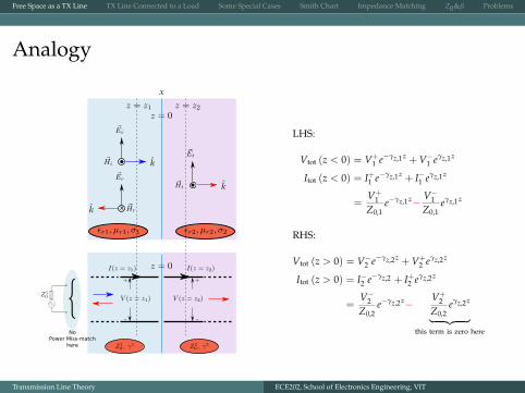
Analogy

x

No Power Miss-match

here

+

-

+

-

LHS:

Vtot (z < 0) = V+1 e−γz,1z + V−1 eγz,1z

Itot (z < 0) = I+1 e−γz,1z + I−1 eγz,1z

=V+

1Z0,1

e−γz,1z− V−1Z0,1

eγz,1z

RHS:

Vtot (z > 0) = V−2 e−γz,2z + V+2 eγz,2z

Itot (z > 0) = I−2 e−γz,2 + I+2 eγz,2z

=V−2Z0,2

e−γz,2z− V+2

Z0,2eγz,2z

︸︷︷︸this term is zero here



Outline




4 Smith Chart


6 Z0&β

7 Problems



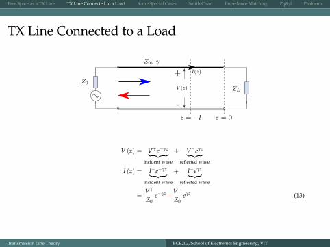
TX Line Connected to a Load

+

-

V (z) = V+e−γz︸︷︷︸incident wave

+ V−eγz︸︷︷︸reflected wave

I (z) = I+e−γz︸︷︷︸incident wave

+ I−eγz︸︷︷︸reflected wave

=V+

Z0e−γz−V−

Z0eγz (13)



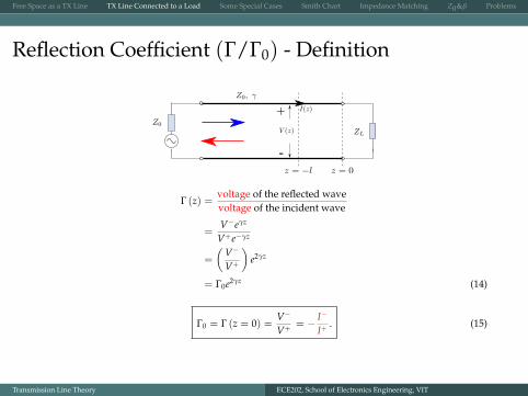
Reflection Coefficient (Γ/Γ0) - Definition

+

-

Γ (z) =voltage of the reflected wavevoltage of the incident wave

=V−eγz

V+e−γz

=

(V−

V+

)e2γz

= Γ0e2γz (14)

Γ0 = Γ (z = 0) =V−

V+= − I−

I+. (15)



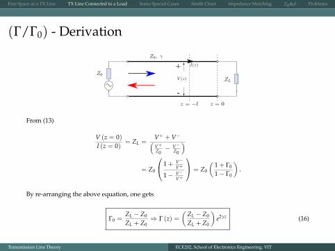
(Γ/Γ0) - Derivation

+

-

From (13)

V (z = 0)I (z = 0)

= ZL =V+ + V−(V+

Z0− V−

Z0

)= Z0

1 + V−V+

1− V−V+

= Z0

(1 + Γ0

1− Γ0

).

By re-arranging the above equation, one gets

Γ0 =ZL − Z0

ZL + Z0⇒ Γ (z) =

(ZL − Z0

ZL + Z0

)e2γz (16)



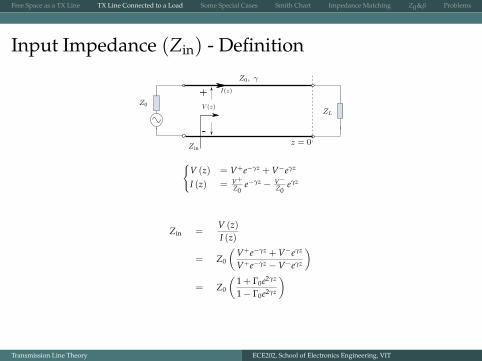
Input Impedance (Zin) - Definition

+

-

V (z) = V+e−γz + V−eγz

I (z) = V+

Z0e−γz − V−

Z0eγz

Zin =V (z)I (z)

= Z0

(V+e−γz + V−eγz

V+e−γz −V−eγz

)= Z0

(1 + Γ0e2γz

1− Γ0e2γz

)



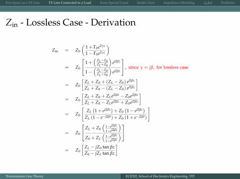
Zin - Lossless Case - Derivation

Zin = Z0

(1 + Γ0e2γz

1− Γ0e2γz

)

= Z0

1 +(

ZL−Z0ZL+Z0

)ej2βz

1−(

ZL−Z0ZL+Z0

)ej2βz

, since γ = jβ, for lossless case

= Z0

[ZL + Z0 + (ZL − Z0) ej2βz

ZL + Z0 − (ZL − Z0) ej2βz

]= Z0

[ZL + Z0 + ZLej2βz − Z0ej2βz

ZL + Z0 − ZLej2βz + Z0ej2βz

]

= Z0

[ZL(1 + ej2βz

)+ Z0

(1− ej2βz

)ZL (1− e−j2βl) + Z0 (1 + e−j2βl)

]

= Z0

ZL + Z0

(1−ej2βz

1+ej2βz

)Z0 + ZL

(1−ej2βz

1+ej2βz

)

= Z0

[ZL − jZ0 tan βzZ0 − jZL tan βz

]



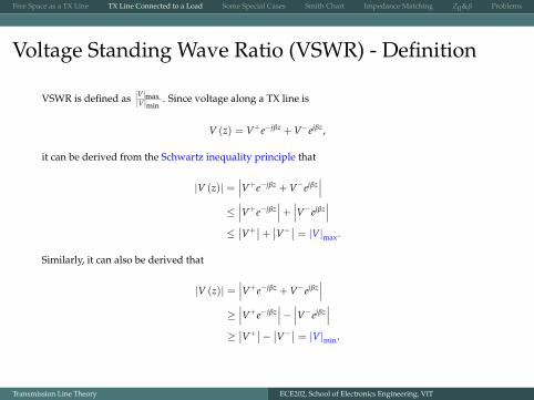
Voltage Standing Wave Ratio (VSWR) - Definition

VSWR is defined as |V|max|V|min

. Since voltage along a TX line is

V (z) = V+e−jβz + V−ejβz,

it can be derived from the Schwartz inequality principle that

|V (z)| =∣∣∣V+e−jβz + V−ejβz

∣∣∣≤∣∣∣V+e−jβz

∣∣∣+ ∣∣∣V−ejβz∣∣∣

≤∣∣V+

∣∣+ ∣∣V−∣∣ = |V|max.

Similarly, it can also be derived that

|V (z)| =∣∣∣V+e−jβz + V−ejβz

∣∣∣≥∣∣∣V+e−jβz

∣∣∣− ∣∣∣V−ejβz∣∣∣

≥∣∣V+

∣∣− ∣∣V−∣∣ = |V|min.



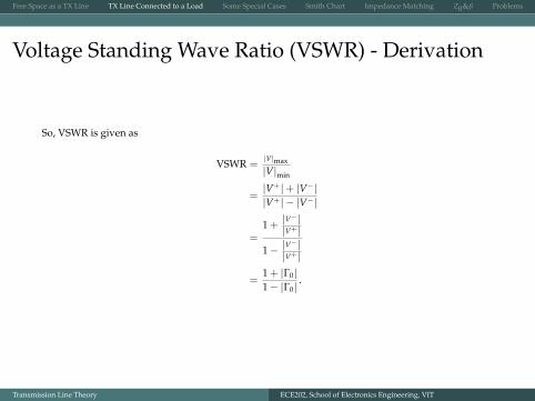
Voltage Standing Wave Ratio (VSWR) - Derivation

So, VSWR is given as

VSWR =|V|max|V|min

=|V+ |+ |V− ||V+ | − |V− |

=1 + |V

− ||V+ |

1− |V− ||V+ |

=1 + |Γ0|1− |Γ0|

.



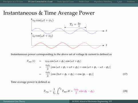
Instantaneous & Time Average Power

Instantaneous power corresponding to the above set of voltage & current is defined as

Pinst (t) = v0i0 cos (ωt + φ1) cos (ωt + φ2)

=v0i0

2[cos (ωt + φ1 + ωt + φ2) + cos (ωt + φ1 −ωt− φ2)]

=v0i0

2[cos (2ωt + φ1 + φ2) + cos (φ1 − φ2)] (17)

Time average power is defined as

Pavg =1

T0

ˆ T0

0Pinst dt =

v0i02

cos (φ1 − φ2) (18)



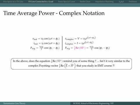
Time Average Power - Complex Notation

vreal = v0 cos (ωt + φ1) vcomplex = V = v0ej(ωt+φ1)

ireal = i0 cos (ωt + φ2) icomplex = I = i0ej(ωt+φ2)

Pavg =v0 i0

2 cos (φ1 − φ2) Pavg = 12 Re (VI∗) = v0 i0

2 cos (φ1 − φ2)

In the above, does the equation 1

2 Re (VI∗) remind you of some thing ? ... Isn’t it very similar to the

complex Poynting vector 12 Re

(~E× ~H∗

)that you study in EMT course ?!



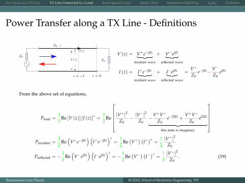
Power Transfer along a TX Line - Definitions

+

-

V (z) = V+e−jβz︸︷︷︸incident wave

+ V−ejβz︸︷︷︸reflected wave

I (z) = I+e−jβz︸︷︷︸incident wave

+ I−ejβz︸︷︷︸reflected wave

=V+

Z0e−jβz−V−

Z0ejβz

From the above set of equations,

Ptotal =12

Re [V (z)] [I (z)]∗ =12

Re

|V+ |2

Z0− |V

− |2

Z0−V+V−

Z0e−j2βz +

V+V−

Z0ej2βz︸︷︷︸

this term is imaginary

Pincident =

12

Re(

V+e−jβz) (

I+e−jβz)∗

=12

Re(V+) (

I+)∗

=12|V+ |2

Z0

Preflected = − 12

Re(

V−ejβz) (

I−ejβz)∗

= − 12

Re(V−) (

I−)∗

=12|V− |2

Z0. (19)



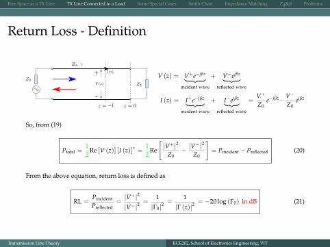
Return Loss - Definition

+

-

V (z) = V+e−jβz︸︷︷︸incident wave

+ V−ejβz︸︷︷︸reflected wave

I (z) = I+e−jβz︸︷︷︸incident wave

+ I−ejβz︸︷︷︸reflected wave

=V+

Z0e−jβz−V−

Z0ejβz

So, from (19)

Ptotal =12

Re [V (z)] [I (z)]∗ =12

Re

[|V+ |2

Z0− |V

− |2

Z0

]= Pincident − Preflected (20)

From the above equation, return loss is defined as

RL =Pincident

Preflected=|V+ |2

|V− |2=

1

|Γ0|2=

1

|Γ (z)|2= −20 log (Γ0) in dB (21)



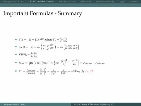
Important Formulas - Summary

• Γ (z = −l) = Γ0e−j2βl, where Γ0 =ZL−Z0ZL+Z0

• Zin (z = −l) = Z0

(1+Γ0e−j2βl

1−Γ0e−j2βl

)= Z0

[ZL+jZ0 tan βlZ0+jZL tan βl

]• VSWR =

1+|Γ0|1−|Γ0|

• Ptotal =12 Re [V (z)] [I (z)]∗ = 1

2 Re[|V+ |2

Z0− |V

− |2Z0

]= Pincident − Preflected

• RL =PincidentPreflected

=|V+ |2

|V− |2= 1

|Γ0|2= 1|Γ(z)|2

= −20 log (Γ0) in dB



Outline




4 Smith Chart


6 Z0&β

7 Problems



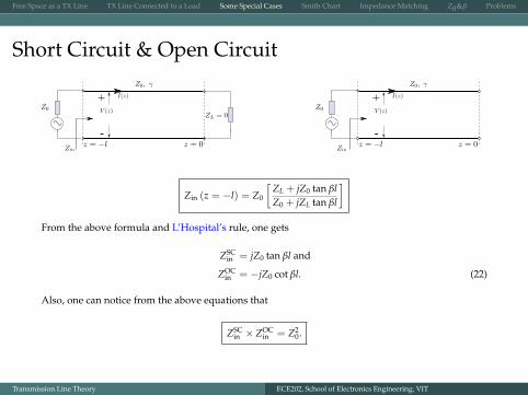
Short Circuit & Open Circuit

+

-

+

-

Zin (z = −l) = Z0

[ZL + jZ0 tan βlZ0 + jZL tan βl

]From the above formula and L’Hospital’s rule, one gets

ZSCin = jZ0 tan βl and

ZOCin = −jZ0 cot βl. (22)

Also, one can notice from the above equations that

ZSCin × ZOC

in = Z20.



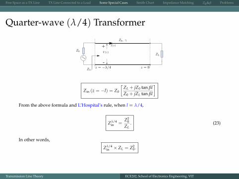
Quarter-wave (λ/4) Transformer

+

-

Zin (z = −l) = Z0

[ZL + jZ0 tan βlZ0 + jZL tan βl

]From the above formula and L’Hospital’s rule, when l = λ/4,

Zλ/4in =

Z20

ZL. (23)

In other words,

Zλ/4in × ZL = Z2

0.



Outline




4 Smith Chart


6 Z0&β

7 Problems



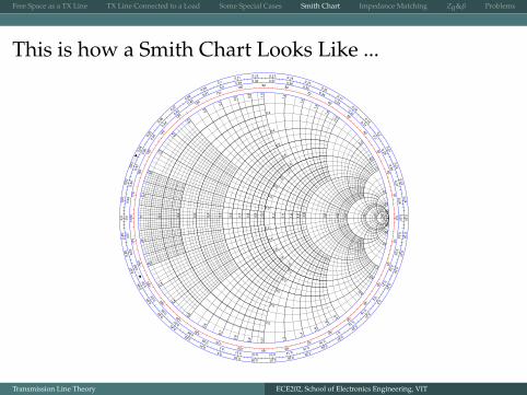
This is how a Smith Chart Looks Like ...



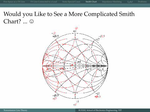
Would you Like to See a More Complicated SmithChart? ... ,



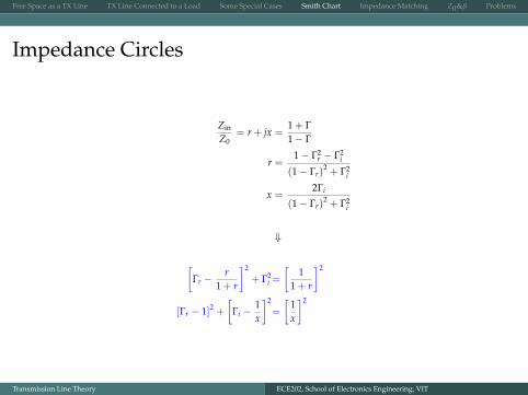
Impedance Circles

Zin

Z0= r + jx =

1 + Γ1− Γ

r =1− Γ2

r − Γ2i

(1− Γr)2 + Γ2

i

x =2Γi

(1− Γr)2 + Γ2

i

⇓

[Γr −

r1 + r

]2

+ Γ2i =

[1

1 + r

]2

[Γr − 1]2 +[

Γi −1x

]2

=

[1x

]2



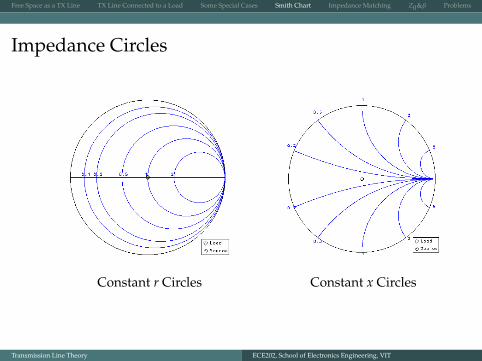
Impedance Circles

Constant r Circles Constant x Circles



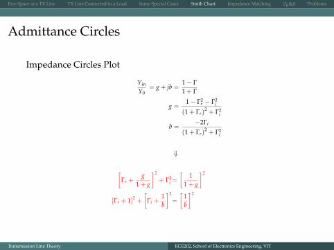
Admittance Circles

Impedance Circles Plot

Yin

Y0= g + jb =

1− Γ1 + Γ

g =1− Γ2

r − Γ2i

(1 + Γr)2 + Γ2

i

b =−2Γi

(1 + Γr)2 + Γ2

i

⇓

[Γr +

g1 + g

]2

+ Γ2i =

[1

1 + g

]2

[Γr + 1]2 +[

Γi +1b

]2

=

[1b

]2



Admittance Circles

Constant g Circles Constant b Circles



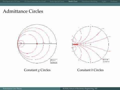
Locating a given Load on the Smith Chart

ZL = 100 + j100Ω, Z0 = 50Ω



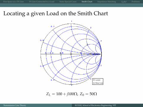
Moving towards the Generator using the ConstantVSWR Circle

Γ (z = −l) = Γ0e−j2βl



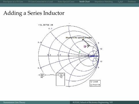
Adding a Series Inductor



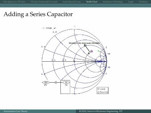
Adding a Series Capacitor



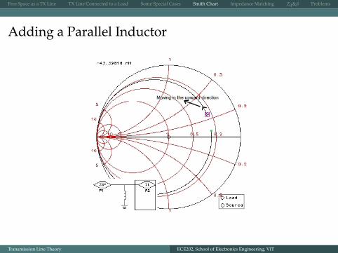
Adding a Parallel Inductor



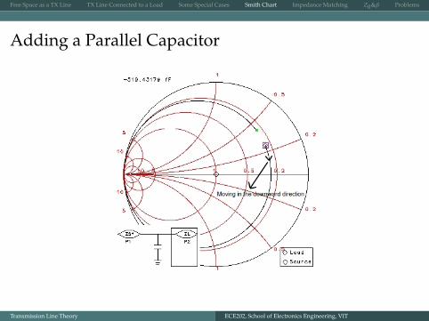
Adding a Parallel Capacitor



Outline




4 Smith Chart


6 Z0&β

7 Problems



For this section, see the PDF file uploaded separately ...



Outline




4 Smith Chart


6 Z0&β

7 Problems



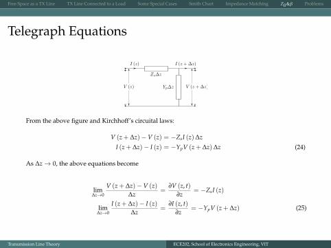
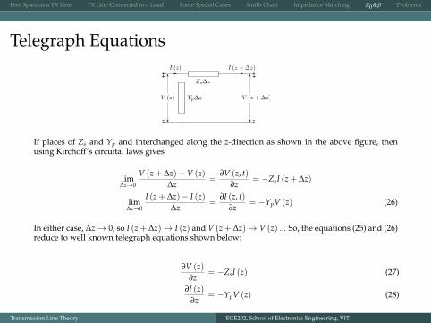
Telegraph Equations

From the above figure and Kirchhoff’s circuital laws:

V (z + ∆z)−V (z) = −ZsI (z)∆z

I (z + ∆z)− I (z) = −YpV (z + ∆z)∆z (24)

As ∆z→ 0, the above equations become

lim∆z→0

V (z + ∆z)−V (z)∆z

=∂V (z, t)

∂z= −ZsI (z)

lim∆z→0

I (z + ∆z)− I (z)∆z

=∂I (z, t)

∂z= −YpV (z + ∆z) (25)



Telegraph Equations

If places of Zs and Yp and interchanged along the z-direction as shown in the above figure, thenusing Kirchoff’s circuital laws gives

lim∆z→0

V (z + ∆z)−V (z)∆z

=∂V (z, t)

∂z= −ZsI (z + ∆z)

lim∆z→0

I (z + ∆z)− I (z)∆z

=∂I (z, t)

∂z= −YpV (z) (26)

In either case, ∆z→ 0; so I (z + ∆z)→ I (z) and V (z + ∆z)→ V (z) ... So, the equations (25) and (26)reduce to well known telegraph equations shown below:

∂V (z)∂z

= −ZsI (z) (27)

∂I (z)∂z

= −YpV (z) (28)



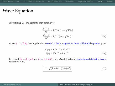
Wave Equation

Substituting (27) and (28) into each other gives

d2V (z)dz2 = ZsYpV (z) = γ2V (z)

d2I (z)dz2 = ZsYpI (z) = γ2I (z) (29)

where γ =√

ZsYp. Solving the above second order homogeneous linear differential equation gives

V (z) = V+e−γz + V−e+γz

I (z) = I+e−γz + I−e+γz. (30)

In general, ZS = R + jωL and YP = G + jωC, where R and G indicate conductor and dielectric losses,respectively. So,

γ =√(R + jωL) (G + jωC) (31)



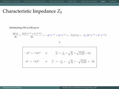
Characteristic Impedance Z0

Substituting (30) in (28) gives

∂I (z)∂z

=∂ (I+e−γz + I−e+γz)

∂z= −γI+e−γz + γI−e+γz = −YpV (z) = −Yp

(V+e−γz + V−e+γz)

⇓

−γI+ = −YpV+ ⇒ V+

I+= γ

YP=√

ZsYp

=√

R+jωLG+jωC = Z0

γI− = −YpV− ⇒ V−I− = − γ

YP= −

√ZsYp

= −√

R+jωLG+jωC = −Z0



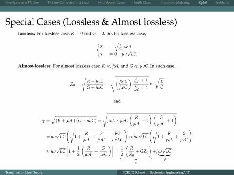
Special Cases (Lossless & Almost lossless)lossless: For lossless case, R = 0 and G = 0. So, for lossless case,

Z0 =

√LC and

γ = 0 + jω√

LC.

Almost-lossless: For almost lossless case, R jωL and G jωC. In such case,

Z0 =

√R + jωLG + jωC

=

√√√√( jωLjωC

) RjωL + 1G

jωC + 1≈√

LC

and

γ =√(R + jωL) (G + jωC) =

√jωL× jωC

(R

jωL+ 1)(

GjωC

+ 1)

= jω√

LC

(√1 +

RjωL

+G

jωC− RG

ω2LC

)≈ jω

√LC

(√1 +

RjωL

+G

jωC

)

≈ jω√

LC[

1 +12

(R

jωL+

GjωC

)]=

12

(RZ0

+ GZ0

)︸︷︷︸

α

+j ω√

LC︸︷︷︸β



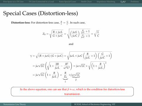
Special Cases (Distortion-less)Distortion-less: For distortion-less case, R

L = GC . In such case,

Z0 =

√R + jωLG + jωC

=

√√√√( jωLjωC

) RjωL + 1G

jωC + 1=

√LC

and

γ =√(R + jωL) (G + jωC) =

√jωL× jωC

(R

jωL+ 1)(

GjωC

+ 1)

= jω√

LC

(√1 +

2RjωL− R2

ω2L2

)= jω

√LC×

√(1 +

RjωL

)2

= jω√

LC(

1 +R

jωL

)=

RZ0︸︷︷︸

α

+j ω√

LC︸︷︷︸β

In the above equation, one can see that β ∝ ω, which is the condition for distortion-less

transmission.



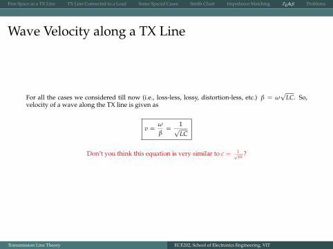
Wave Velocity along a TX Line

For all the cases we considered till now (i.e., loss-less, lossy, distortion-less, etc.) β = ω√

LC. So,velocity of a wave along the TX line is given as

v =ω

β=

1√LC

Don’t you think this equation is very similar to c = 1√µε ?



Outline




4 Smith Chart


6 Z0&β

7 Problems



Transmission Lines - Basics



Smith Chart - Problems



Transmission Line - Lumped Element Model


Transmission Line Theory - Arraytool · Free Space as a TX LineTX Line Connected to a LoadSome...

Documents

Transcript of Transmission Line Theory - Arraytool · Free Space as a TX LineTX Line Connected to a LoadSome...

Transmission Line Theory - Arraytool · 5/4/2015 · Transmission Line Theory ECE202, School of Electronics Engineering, VIT. Free Space as a TX LineTX Line Connected to a LoadSome

Transmission problems and spectral theory for singular ...faculty.missouri.edu/~mitream/luismarius_veryshort.pdf · Transmission problems and spectral theory for singular integral

Optical Transmission Basics

Noradrenergic transmission

Understanding Transmission Lines · Understanding Transmission Lines 8/8/2012 Larry Benko, W0QE 1

11 Transmission Lines

Playtime: Macklin Kowal @Automatic Transmission · 2019. 11. 27. · Playtime: Macklin Kowal @Automatic Transmission Macklin Kowal collaborates with Automatic Transmission in the

Transmission Lines - Engineeringece.uprm.edu/~pol/pdf/4transmissionLines.pdf · Common Transmission Lines R, L, G, and C depend on the particular transmission line structure and the

17: Transmission Lines - Imperial College · PDF file17: Transmission Lines 17: ... • Transmission Lines • Transmission Line ... δx is the total inductance per unit length

The Friis Transmission Formulausers.cecs.anu.edu.au/~Gerard.Borg/anu/courses/... · The Friis Transmission Formula If we assume that the antennas are aligned for maximum transmission

Transmission Linespol/pdf/transmissionLines.pdftransformer, Slotted line, Single stub VI. Microstrips Transmission Lines (TL) n TL have 2 conductors in parallel with a dielectric separating

14 - Transmission-line losses in the mm / THz rangeantena.fe.uni-lj.si/literatura/Razno/Konferenca midem 2015/mm2.pdf · Transistor (BJT or FET ... Terahertz emission and detection

1- A lossless transmission line of characteristic …eem.eskisehir.edu.tr/cozzaim/EEM 509/icerik/example3.pdf6- A dipole antenna consisting of two highly conductive circular rods of

B. The Terminated, Lossless Transmission Line - KU ITTC · 8/27/2007 The Terminated Transmission Line notes 1/2 Jim Stiles The Univ. of Kansas Dept. of EECS B. The Terminated, Lossless

Transmission Line (TL) Approach of Left-Handed (LH) Materialsxlab.me.berkeley.edu/muri/Kickoff/Jan25/Itoh.pdf · 2012-07-11 · Microwave Electronics Lab LH-TL as the Dual of the

ELG 4125: ELECTRICAL POWER TRANSMISSION AND …rhabash/ELG4125DGD32007.pdf · 3) A 3-phase, 50 Hz transmission line 100 km long delivers 20 MW at 0·9 p.f. lagging and at 110 kV.

Transmission problems and spectral theory for singular ... · Transmission problems and spectral theory for singular integral operators on Lipschitz domains Luis Escauriaza and Marius

Transmission Line Reviewwebpages.iust.ac.ir/nayyeri/Courses/MCD/Lecture_2.pdfGiven a 50 Ω transmission line that is 0.25 λ long excited by a 1 V voltage source at 300 MHz frequency

1 Chapter 2. Transmission Line Theory Sept. 29 th, 2008.

Accounting for High Frequency Transmission Line Loss ...data.eefocus.com/myspace/1/8760/bbs/1187796227/c051a58.pdf · Accounting for High Frequency Transmission Line Loss Effects