
Trade Elasticity
41
Trade Elasticity Jos´ e de Sousa and Isabelle Mejean Topics in International Trade University Paris-Saclay Master in Economics, 2nd year
Transcript of Trade Elasticity
Trade Elasticity
Jose de Sousa and Isabelle Mejean
Topics in International Trade
University Paris-Saclay Master in Economics, 2nd year
Motivation : Trade Elasticity
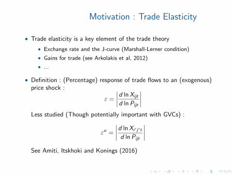
• Trade elasticity is a key element of the trade theory
• Exchange rate and the J-curve (Marshall-Lerner condition)
• Gains for trade (see Arkolakis et al, 2012)
• ...
• Definition : (Percentage) response of trade flows to an (exogenous)price shock :
ε =
∣∣∣∣d lnXijt
d lnPijt
∣∣∣∣
Less studied (Though potentially important with GVCs) :
εo =
∣∣∣∣d lnXi ′j′t
d lnPijt
∣∣∣∣
See Amiti, Itskhoki and Konings (2016)
Empirical Evidence on Trade Elasticities
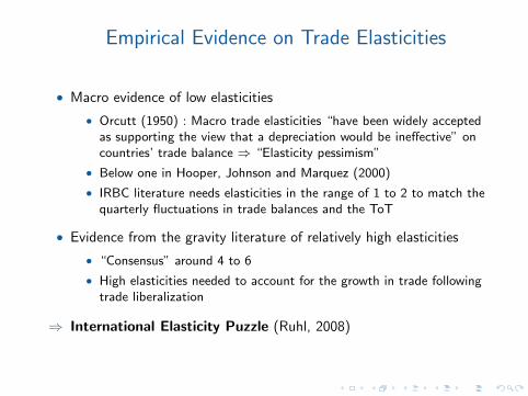
• Macro evidence of low elasticities
• Orcutt (1950) : Macro trade elasticities “have been widely acceptedas supporting the view that a depreciation would be ineffective” oncountries’ trade balance ⇒ “Elasticity pessimism”
• Below one in Hooper, Johnson and Marquez (2000)
• IRBC literature needs elasticities in the range of 1 to 2 to match thequarterly fluctuations in trade balances and the ToT
• Evidence from the gravity literature of relatively high elasticities
• “Consensus” around 4 to 6
• High elasticities needed to account for the growth in trade followingtrade liberalization
⇒ International Elasticity Puzzle (Ruhl, 2008)
Empirical difficulties
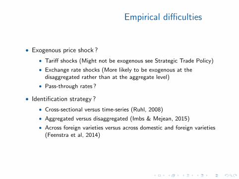
• Exogenous price shock ?
• Tariff shocks (Might not be exogenous see Strategic Trade Policy)
• Exchange rate shocks (More likely to be exogenous at thedisaggregated rather than at the aggregate level)
• Pass-through rates ?
• Identification strategy ?
• Cross-sectional versus time-series (Ruhl, 2008)
• Aggregated versus disaggregated (Imbs & Mejean, 2015)
• Across foreign varieties versus across domestic and foreign varieties(Feenstra et al, 2014)
Road Map
• Estimating trade elasticities
• From micro to macro elasticities
Estimating Trade Elasticities
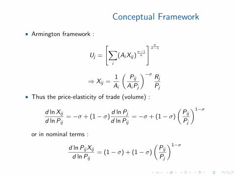
Conceptual Framework
• Armington framework :
Uj =
[∑
i
(AiXij)σ−1σ
] σσ−1
⇒ Xij =1
Ai
(Pij
AiPj
)−σRj
Pj
• Thus the price-elasticity of trade (volume) :
d lnXij
d lnPij= −σ + (1− σ)
d lnPj
d lnPij= −σ + (1− σ)
(Pij
Pj
)1−σ
or in nominal terms :
d lnPijXij
d lnPij= (1− σ) + (1− σ)
(Pij
Pj
)1−σ

Conceptual Framework
• Above definition holds true in a large class of models (see Head andMayer, 2013)
• “Gravity-type” models which assume i) a constant price elasticity
(d ln Xij
d ln Pij= cst) ii) no “third country effects” (
d ln Xij
d ln Pi′ j= 0 ∀i , i ′)
• Most of the time, monopolistic/perfect competition implies(Pij/Pj)
1−σ ≈ 0
⇒ Trade elasticities can be estimated in the cross-section of countriesand/or over time
• Not in every model : See eg Novy (2013) :
• With translog preferences (thus variable mark-ups), the tradeelasticity becomes :
εij =γni
Xij/Yj
Neither constant over time, nor across country pairs !

Empirical Framework
• From the previous conceptual framework :
d lnXijt = −ε d lnPijt + Controlsijt + uijt
where ε can be estimated across country pairs and/or over time
• Problem : Prices are not exogenous to quantities
• IV strategy
• Structural estimation of a demand-supply model (Feenstra, 1994)
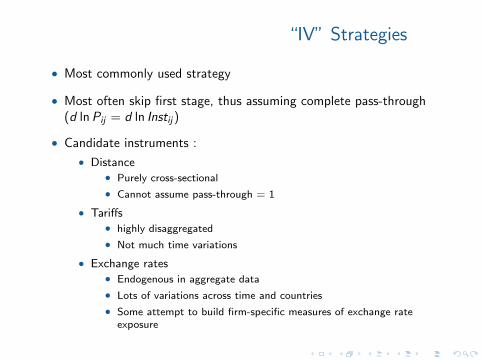
“IV” Strategies
• Most commonly used strategy
• Most often skip first stage, thus assuming complete pass-through(d lnPij = d ln Instij)
• Candidate instruments :
• Distance• Purely cross-sectional
• Cannot assume pass-through = 1
• Tariffs• highly disaggregated
• Not much time variations
• Exchange rates• Endogenous in aggregate data
• Lots of variations across time and countries
• Some attempt to build firm-specific measures of exchange rateexposure
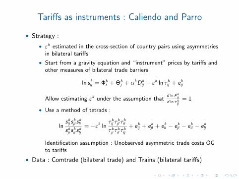
Tariffs as instruments : Caliendo and Parro
• Strategy :
• εk estimated in the cross-section of country pairs using asymmetriesin bilateral tariffs
• Start from a gravity equation and “instrument” prices by tariffs andother measures of bilateral trade barriers
ln skij = Φki + Θk
j + αkDkij − εk ln τ kij + ekij
Allow estimating εk under the assumption thatd ln Pk
ij
d ln τkij
= 1
• Use a method of tetrads :
lnskij s
kjl s
kli
skji skil s
klj
= −εk lnτ kij τ
kjl τ
kli
τ kji τkil τ
klj
+ ekij + ekjl + ekli − ekji − ekil − eklj
Identification assumption : Unobserved asymmetric trade costs OGto tariffs
• Data : Comtrade (bilateral trade) and Trains (bilateral tariffs)
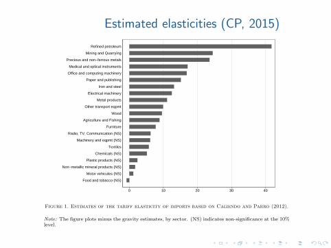
Estimated elasticities (CP, 2015)VOL. VOL NO. ISSUE ELASTICITY OPTIMISM 21
0 10 20 30 40
Food and tobacco (NS)
Motor vehicules (NS)
Non−metallic mineral products (NS)
Plastic products (NS)
Chemicals (NS)
Textiles
Machinery and eqpmt (NS)
Radio, TV, Communication (NS)
Furniture
Agriculture and Fishing
Wood
Other transport eqpmt
Metal products
Electrical machinery
Iron and steel
Paper and publishing
Office and computing machinery
Medical and optical instruments
Precious and non−ferrous metals
Mining and Quarrying
Refined petroleum
Figure 1. Estimates of the tariff elasticity of imports based on Caliendo and Parro (2012).
Note: The figure plots minus the gravity estimates, by sector. (NS) indicates non-significance at the 10%level.
Broda and Weinstein (2006) implement a similar estimation on 243 SITC-3 sectorsbetween 1972 and 1988, with mean −4.9, and median −2.0. Their mean estimateis close to the one presented here. Their median estimate is closer to zero thanours, reflecting the differences in classifications in both exercises.25
Are the sector-level estimates in this paper comparable with those obtainedin the literature more generally? Houthakker and Magee (1969) report in Table6 a median import price elasticity in manufactures estimated at −4.05. This isvirtually identical to the median value obtained here across 56 manufacturingsectors. Similarly, Kreinin (1967) documents an elasticity for manufactures equalto −4.71. Interestingly, both papers make use of information on the prices ofdomestic goods to estimate the Armington elasticity. This paper does not, andit is reassuring that the estimates obtained with either data should be close.
Both sets of estimates confirm that sector-level elasticities are heterogeneousand relatively high on average. There is little doubt that such is the case in theliterature. Romalis (2007) estimates elasticities between −3 and −12 at the HS6
25The gravity estimation yields large elasticity values, just like the meta-analysis in Head and Mayer(2014): Their Table 5 indicates that gravity estimates are systematically larger in absolute value thanthose obtained if changes in import prices are instrumented with changes in wages, in observed prices,or in exchange rates.

Tariffs as instruments : Head and Ries
• Strategy :
• εk estimated in the cross-section of importers, using panel data
• Start from a gravity equation and “instrument” prices by tariffs andother measures of bilateral trade barriers
ln bkjt = εk lnNTBk
t︸ ︷︷ ︸FEt
−εk ln τ kjt + (FEk) + ekjt
bkjt the relative advantage of domestic against imported goods in
country j Allow estimating εk under the assumption thatd ln Pk
jt
d ln τkjt
= 1
Identification assumption : Unobserved country-specific trade costsOG to tariffs
• Data : Industry Canada at the SIC level (manufacturing)
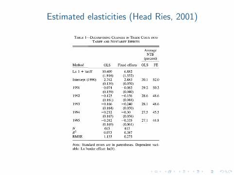
Estimated elasticities (Head Ries, 2001)864 THE AMERICAN ECONOMIC REVIEW SEPTEMBER 2001
where TAR and NTB represent the ad valorem rates of tariffs and nontariff barriers. We define NTB to comprise all barriers to export success other than tariffs, including transportation costs, home bias (h), and any government policies that favor domestically produced goods over imports. Other authors using different method- ologies have estimated the overall border effect (John McCallum, 1995; John F. Helliwell, 1996; Shang-Jin Wei, 1996) but have not de- composed it into tariff and nontariff barrier components. Denoting industries with i and years with t, note that we observe TARit (see the Data Appendix) but must infer NTBit as a residual. We assume that (u- - 1)ln(1 + NTBit) can be approximated as (u - l)ln(1 + NTBt) + 8it. Substituting, we obtain a log linear regression equation:
(10) ln(bit) = (o- 1)ln(1 + NTBt)
+ (- - 1)ln(1 + TARit) + 8it.
We estimate the first term with year dummies. Note that almost any border effect can be ob- tained from tiny tariff barriers if the elasticity of substitution o- is high enough.
Column (1) of Table 1 presents results for ordinary least-squares (OLS) estimation, whereas colunm (2) reflects results when we add industry fixed effects. The coefficient on the tariff variable implies that the elasticity of substitution between goods o- ranges between 7.9 (fixed effects) and 11.4 (pooled OLS). The reduction in estimated o- caused by controlling for industry-specific effects suggests that the OLS estimate is upwardly biased because of a positive correlation between tariff levels and fixed, unmeasured characteristics of industries that raise bit. Although even the fixed- effects estimate of o- may appear high, it is con- sistent with results in several other recent studies. Feenstra (1994) estimates price elasticities for a demand and supply system using a panel of ex- porting countries over the years 1964-1987. He obtains 95-percent confidence intervals for six products with an average lower bound of 3.9 and average upper bound of 8.8.6 Scott L. Baier and
TABLE 1-DECOMPOSING CHANGES IN TRADE COSTS INTO TARIFF AND NONTARIFF EFFECTS
Average NTB
(percent)
Method OLS Fixed effects OLS FE
Ln 1 + tariff 10.409 6.882 (1.916) (1.532)
Intercept (1990) 2.742 2.883 30.1 52.0 (0.139) (0.070)
1991 -0.074 -0.082 29.2 50.2 (0.159) (0.040)
1992 -0.123 -0.156 28.6 48.6 (0.161) (0.044)
1993 -0.166 -0.240 28.1 48.6 (0.164) (0.050)
1994 -0.212 -0.30 27.5 45.5 (0.167) (0.056)
1995 -0.242 -0.335 27.1 44.8 (0.169) (0.061)
N 615 615 R2 0.073 0.387 RMSE 1.133 0.275
Note: Standard errors are in parentheses. Dependent vari- able: Ln border effect: ln(b).
Jeffrey H. Bergstrand (2001) fit a gravity equation to bilateral trade between 16 industrialized coun- tries. They obtain a point estimate for the elasticity of substitution equal to 6.43 with a 90- percent confidence interval of [2.44, 10.4]. David Hummels (1998) calculates o- equal to 7.6 using information on how freight costs affect trade. Us- ing a methodology based on geographic variation in wages, Gordon H. Hanson (1998) obtains esti- mates of o- that range between 6 and 11. Jonathan Eaton and Samuel Kortum (1998) estimate a model based on technology differences but obtain a value of 8.3 for a parameter that is observation- ally equivalent to our o-.
Our estimates tend to be higher than those obtained from directly estimating import price elasticities. For example, Bruce A. Blonigen and Wesley W. Wilson (1999) report an average elasticity across 146 three-digit sectors of just 0.81. They obtain their estimates by regressing the ratio of imports to domestic output on the import/domestic price ratio using quarterly U.S. data for the period 1980-1988. There are four
6 The six products and their 95-percent confidence inter- vals are men's leather athletic shoes [4.4, 10.6], men's and boy's cotton knit shirts [4.2, 11.0], stainless steel bars [2.8,
5.3], carbon steel sheets [3.0, 10.0], color TV receivers [6.4, 12.3], and portable typewriters [2.5, 3.6].
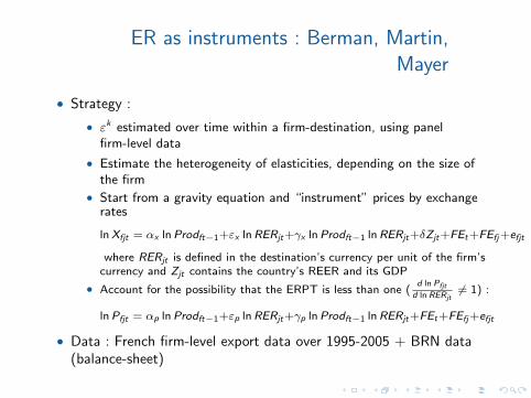
ER as instruments : Berman, Martin,Mayer
• Strategy :
• εk estimated over time within a firm-destination, using panelfirm-level data
• Estimate the heterogeneity of elasticities, depending on the size ofthe firm
• Start from a gravity equation and “instrument” prices by exchangerates
lnXfjt = αx lnProdft−1+εx lnRERjt+γx lnProdft−1 lnRERjt+δZjt+FEt+FEfj+efjt
where RERjt is defined in the destination’s currency per unit of the firm’scurrency and Zjt contains the country’s REER and its GDP
• Account for the possibility that the ERPT is less than one (d ln Pfjt
d ln RERjt6= 1) :
lnPfjt = αp lnProdft−1+εp lnRERjt+γp lnProdft−1 lnRERjt+FEt+FEfj+efjt
• Data : French firm-level export data over 1995-2005 + BRN data(balance-sheet)
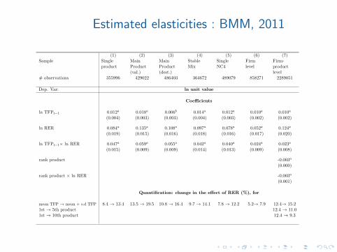
Estimated elasticities : BMM, 2011Table III: Baseline Results
(1) (2) (3) (4) (5) (6) (7)Sample Single
productMainProduct(val.)
MainProduct(dest.)
StableMix
SingleNC4
Firmlevel
Firm-productlevel
# observations 355996 429022 486403 364672 489079 858271 2289051
Dep. Var: ln unit value
Coefficients
ln TFPt−1 0.012a 0.018a 0.006b 0.014a 0.012a 0.010a 0.010a
(0.004) (0.003) (0.003) (0.004) (0.003) (0.002) (0.002)
ln RER 0.084a 0.135a 0.108a 0.097a 0.078a 0.052a 0.124a
(0.019) (0.015) (0.016) (0.018) (0.016) (0.017) (0.020)
ln TFPt−1× ln RER 0.047a 0.059a 0.055a 0.042a 0.040a 0.024a 0.023a
(0.015) (0.009) (0.009) (0.014) (0.013) (0.009) (0.008)
rank product -0.003a
(0.000)
rank product × ln RER -0.003a
(0.001)
Quantification: change in the effect of RER (%), for
mean TFP → mean + s.d TFP 8.4 → 13.4 13.5 → 19.5 10.8 → 16.4 9.7 → 14.1 7.8 → 12.2 5.2→ 7.9 12.4→ 15.21st → 5th product 12.4 → 11.01st → 10th product 12.4 → 9.3
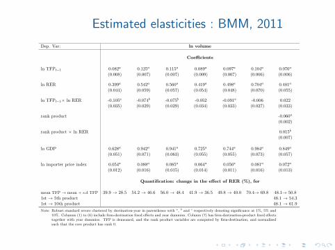
Dep. Var: ln volume
Coefficients
ln TFPt−1 0.082a 0.125a 0.115a 0.089a 0.097a 0.104a 0.076a
(0.008) (0.007) (0.007) (0.009) (0.007) (0.006) (0.006)
ln RER 0.399a 0.542a 0.560a 0.419a 0.498a 0.704a 0.481a
(0.044) (0.059) (0.057) (0.054) (0.048) (0.070) (0.055)
ln TFPt−1× ln RER -0.105a -0.074b -0.075b -0.052 -0.091a -0.006 0.022(0.035) (0.029) (0.029) (0.034) (0.033) (0.027) (0.033)
rank product -0.060a
(0.002)
rank product × ln RER 0.015b
(0.007)
ln GDP 0.628a 0.942a 0.941a 0.725a 0.744a 0.984a 0.849a
(0.051) (0.071) (0.063) (0.055) (0.055) (0.073) (0.057)
ln importer price index 0.054a 0.088a 0.085a 0.064a 0.056a 0.081a 0.072a
(0.012) (0.016) (0.015) (0.014) (0.011) (0.016) (0.013)
Quantification: change in the effect of RER (%), for
mean TFP → mean + s.d TFP 39.9 → 28.5 54.2 → 46.6 56.0 → 48.4 41.9 → 36.5 49.8 → 40.0 70.4→ 69.8 48.1→ 50.81st → 5th product 48.1 → 54.31st → 10th product 48.1 → 61.9
Note: Robust standard errors clustered by destination-year in parentheses with a, b and c respectively denoting significance at 1%, 5% and10%. Columns (1) to (6) include firm-destination fixed effects and year dummies. Column (7) has firm-destination-product fixed effectstogether with year dummies. TFP is demeaned, and the rank product variables are computed by firm-destination, and normalizedsuch that the core product has rank 0.
13
Estimated elasticities : BMM, 2011
Table III: Baseline Results
(1) (2) (3) (4) (5) (6) (7)Sample Single
productMainProduct(val.)
MainProduct(dest.)
StableMix
SingleNC4
Firmlevel
Firm-productlevel
# observations 355996 429022 486403 364672 489079 858271 2289051
Dep. Var: ln unit value
Coefficients
ln TFPt−1 0.012a 0.018a 0.006b 0.014a 0.012a 0.010a 0.010a
(0.004) (0.003) (0.003) (0.004) (0.003) (0.002) (0.002)
ln RER 0.084a 0.135a 0.108a 0.097a 0.078a 0.052a 0.124a
(0.019) (0.015) (0.016) (0.018) (0.016) (0.017) (0.020)
ln TFPt−1× ln RER 0.047a 0.059a 0.055a 0.042a 0.040a 0.024a 0.023a
(0.015) (0.009) (0.009) (0.014) (0.013) (0.009) (0.008)
rank product -0.003a
(0.000)
rank product × ln RER -0.003a
(0.001)
Quantification: change in the effect of RER (%), for
mean TFP → mean + s.d TFP 8.4 → 13.4 13.5 → 19.5 10.8 → 16.4 9.7 → 14.1 7.8 → 12.2 5.2→ 7.9 12.4→ 15.21st → 5th product 12.4 → 11.01st → 10th product 12.4 → 9.3
Dep. Var: ln volume
Coefficients
ln TFPt−1 0.082a 0.125a 0.115a 0.089a 0.097a 0.104a 0.076a
(0.008) (0.007) (0.007) (0.009) (0.007) (0.006) (0.006)
ln RER 0.399a 0.542a 0.560a 0.419a 0.498a 0.704a 0.481a
(0.044) (0.059) (0.057) (0.054) (0.048) (0.070) (0.055)
ln TFPt−1× ln RER -0.105a -0.074b -0.075b -0.052 -0.091a -0.006 0.022(0.035) (0.029) (0.029) (0.034) (0.033) (0.027) (0.033)
rank product -0.060a
(0.002)
rank product × ln RER 0.015b
(0.007)
ln GDP 0.628a 0.942a 0.941a 0.725a 0.744a 0.984a 0.849a
(0.051) (0.071) (0.063) (0.055) (0.055) (0.073) (0.057)
ln importer price index 0.054a 0.088a 0.085a 0.064a 0.056a 0.081a 0.072a
(0.012) (0.016) (0.015) (0.014) (0.011) (0.016) (0.013)
Quantification: change in the effect of RER (%), for
mean TFP → mean + s.d TFP 39.9 → 28.5 54.2 → 46.6 56.0 → 48.4 41.9 → 36.5 49.8 → 40.0 70.4→ 69.8 48.1→ 50.81st → 5th product 48.1 → 54.31st → 10th product 48.1 → 61.9
Note: Robust standard errors clustered by destination-year in parentheses with a, b and c respectively denoting significance at 1%, 5% and10%. Columns (1) to (6) include firm-destination fixed effects and year dummies. Column (7) has firm-destination-product fixed effectstogether with year dummies. TFP is demeaned, and the rank product variables are computed by firm-destination, and normalizedsuch that the core product has rank 0.
13
Estimated elasticities : BMM, 2011
• Assumption of complete pass-through is counterfactual
• ER adjustments are not passed-through one-to-one into prices
• Firms reduce their mark-up when facing an appreciation of theircurrency
• More so the largest they are
• Consistent with pricing-to-market behaviours (Krugman, 1987)
• When regressing exports on exchange rates, one estimates theproduct of the price elasticity and the pass-through rate :
lnXij = ε lnPij = εγ lnRERij
• Exports flows are (little) responsive to ER movements
• This does not mean that trade elasticities are low
• Response of trade flows to ER movements is even smaller for highproductive firms
• Rationalized in a model of trade with additive trade costs
ER versus tariffs as instruments :Fitzgerald & Haller
• Strategy :
• Use firm-destination panel data to estimate the elasticity of trade toboth tariffs and ERs
• Estimated equation :
Pr [Xfjt > 0] = FEj + FEft + α lnRERjt + β ln τkjt + Xkjt + efjt
lnPfjtXfjt = FEj + FEft + α lnRERjt + β ln τkjt + Xkjt + efjt
with k the sector of activity of firm f
• Data : Irish firm-level export and total revenues data over 1996-2009
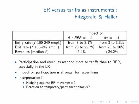
ER versus tariffs as instruments :Fitzgerald & Haller
Impact ofd lnRER = −.1 dτ = −.1
Entry rate (f 100-249 empl.) from 3 to 3.1% from 3 to 3.3%Exit rate (f 100-249 empl.) from 23 to 22.7% from 23 to 20%Revenues (median f ) +6.4% +24.2%
• Participation and revenues respond more to tariffs than to RER,especially in the LR
• Impact on participation is stronger for larger firms
• Interpretation ?• Hedging against ER movements ?• Reaction to temporary/permanent shocks ?
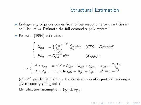
Structural Estimation
• Endogeneity of prices comes from prices responding to quantities inequilibrium ⇒ Estimate the full demand-supply system
• Feenstra (1994) estimates :
Xijkt =(
Pijkt
Pjkt
)−σk
Rjkt
Pjkteuijkt (CES − Demand)
Pijkt = Xωk
1−ωk
ijkt evijkt (Supply)
⇒
d ln sijkt = εkd lnPijkt + Φjkt + ξijkt , sijkt ≡ PijktXijkt
Rjkt
d lnPijkt = ωkd ln sijkt + Ψjkt + δijkt , εk ≡ 1− σk
(εk , ωk) jointly estimated in the cross-section of exporters i serving agiven country j in good k
Identification assumption : ξijkt ⊥ δijkt
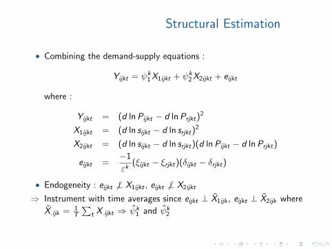
Structural Estimation
• Combining the demand-supply equations :
Yijkt = ψk1X1ijkt + ψk
2X2ijkt + eijkt
where :
Yijkt = (d lnPijkt − d lnPrjkt)2
X1ijkt = (d ln sijkt − d ln srjkt)2
X2ijkt = (d ln sijkt − d ln srjkt)(d lnPijkt − d lnPrjkt)
eijkt =−1
εk(ξijkt − ξrjkt)(δijkt − δrjkt)
• Endogeneity : eijkt 6⊥ X1ijkt , eijkt 6⊥ X2ijkt
⇒ Instrument with time averages since eijkt ⊥ X1ijk , eijkt ⊥ X2ijk where
X.ijk = 1T
∑t X.ijkt ⇒ ψk
1 and ψk2
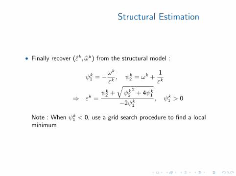
Structural Estimation
• Finally recover (εk , ωk) from the structural model :
ψk1 = −ω
k
εk, ψk
2 = ωk +1
εk
⇒ εk =ψk
2 +
√ψk
22
+ 4ψk1
−2ψk1
, ψk1 > 0
Note : When ψk1 < 0, use a grid search procedure to find a local
minimum
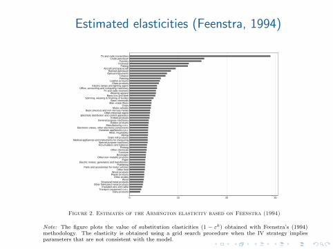
Estimated elasticities (Feenstra, 1994)22 AMERICAN ECONOMIC JOURNAL MONTH 2014
0 10 20 30
Dairy productsTransport equipment n.e.c.
Insulated wire and cableOther fabricated metal products
Structural metal productsWood
Other textilesPlastic productsWood products
Other foodParts and accessories for motor vehicles
PublishingElectric motors, generators and transformers
PaperOther non−metallic products
BeveragesFurniture
Other chemicalsPrinting
Accumulators and batteriesSpecial purpose machinery
Medical appliances and instruments for measuringGrain mill products
MiningMeat, Vegetables
Domestic appliances n.e.c.Electronic valves, other electronic components
Manufacturing n.e.c.Rubber products
General purpose machineryKnitted products
Electricity distribution and control apparatusOther electrical eqpmt
Basic precious and non−ferrous metalsMotor vehicles
CropsMan−made fibres
Basic chemicalsSpinning, weaving & finishing of textiles
Basic iron and steelWearing apparel
TV and radio receiversOffice, accounting and computing machinery
Electric lamps and lighting eqpmtGlass products
Leather productsFarmingTobacco
Optical instrumentsRefined petroleum
Aircraft and spacecraftFishing
FootwearForestry
Crude petroleumTV and radio transmitters
Figure 2. Estimates of the Armington elasticity based on Feenstra (1994)
Note: The figure plots the value of substitution elasticities (1 − εk) obtained with Feenstra’s (1994)methodology. The elasticity is obtained using a grid search procedure when the IV strategy impliesparameters that are not consistent with the model.
level. Head and Ries (2001) report values between −6.9 and −10.4 at the 3-digitSIC level. Hummels (2001) obtains values between −2 and −7 in two-digit data.A key contention in this paper is that sectoral estimates are high on average,and that they decrease with the level of aggregation. This has to be true if aheterogeneity bias is to explain the elasticity puzzle. The claim is supported bythe meta-analysis in Disdier and Head (2008), who consider estimates of the effectof distance on trade flows. They find an index capturing the level of disaggregationis systematically positive, so that average sectoral estimates fall with the level ofaggregation.26 Hummels (2001) finds estimates of the elasticity fall from −3.8to −7.3 as aggregation moves from one- to four-digit. Between 1972 and 1988,Broda and Weinstein (2006) report an average elasticity of −4.9 in SITC3 datawith 243 categories, falling to −10.7 in TSUSA/HTS data with 12,219 categories.
Are there elasticity estimates that are low in sectoral data? Reinert and Roland-Holst (1992) or Blonigen and Wilson (1999) report elasticities for more than 150sectors, with only few values below −2. Gallaway, McDaniel and Rivera (2003)consider 309 US sectors, and find elasticities between −0.5 and −4, averaging−0.55. These are low averages. However, in all three papers the price of imported
26The dispersion in distance coefficients can stem either from heterogeneous import elasticities, orfrom the heterogeneous effects of distance on trade costs.

From Micro to Macro Elasticities

From Micro to Macro Elasticities
• Previous analysis shows elasticities estimated from disaggregated(product or firm-level) data
• Huge amount of heterogeneity in trade elasticities
• Models of international macro/trade usually require to calibrate onetrade elasticity
• Solutions :
• Use aggregate data (see almost 100% of the macro literature) ⇒Problems of endogeneity can be massive
• Use disaggregated data but constrain elasticities to equality acrosssectors (eg Head & Ries, 2001)
• Calibrate multi-sector models (Caliendo & Parro, 2015)
• Aggregate disaggregated elasticities (Imbs & Mejean, 2015)
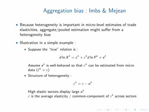
Aggregation bias : Imbs & Mejean
• Because heterogeneity is important in micro-level estimates of tradeelasticities, aggregate/pooled estimation might suffer from aheterogeneity bias
• Illustration in a simple example :
• Suppose the “true” relation is :
d lnX k = ck + εkd lnPk + ek
Assume ek is well-behaved so that εk can be estimated from microdata (εk = ε)
• Structure of heterogeneity :
εk = ε− ok
High elastic sectors display large ok
ε is the average elasticity / common-component of εk across sectors
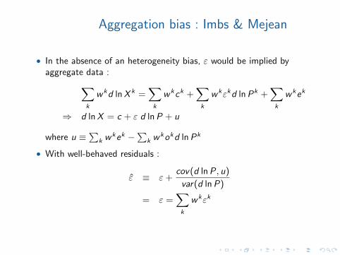
Aggregation bias : Imbs & Mejean
• In the absence of an heterogeneity bias, ε would be implied byaggregate data :
∑
k
wkd lnX k =∑
k
wkck +∑
k
wkεkd lnPk +∑
k
wkek
⇒ d lnX = c + ε d lnP + u
where u ≡∑k wkek −∑k w
kokd lnPk
• With well-behaved residuals :
ε ≡ ε+cov(d lnP, u)
var(d lnP)
= ε =∑
k
wkεk
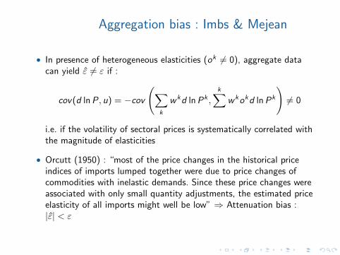
Aggregation bias : Imbs & Mejean
• In presence of heterogeneous elasticities (ok 6= 0), aggregate datacan yield ε 6= ε if :
cov(d lnP, u) = −cov(∑
k
wkd lnPk ,
k∑wkokd lnPk
)6= 0
i.e. if the volatility of sectoral prices is systematically correlated withthe magnitude of elasticities
• Orcutt (1950) : “most of the price changes in the historical priceindices of imports lumped together were due to price changes ofcommodities with inelastic demands. Since these price changes wereassociated with only small quantity adjustments, the estimated priceelasticity of all imports might well be low” ⇒ Attenuation bias :|ε| < ε
Aggregation bias : Imbs & Mejean
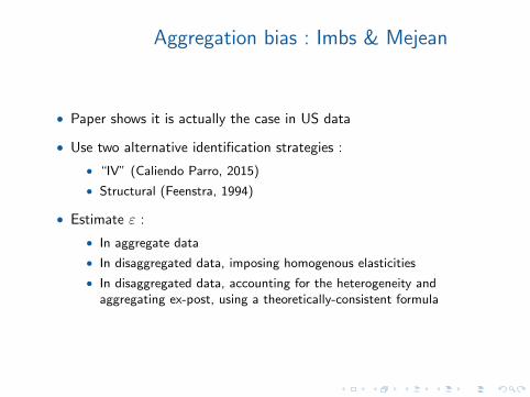
• Paper shows it is actually the case in US data
• Use two alternative identification strategies :
• “IV” (Caliendo Parro, 2015)
• Structural (Feenstra, 1994)
• Estimate ε :
• In aggregate data
• In disaggregated data, imposing homogenous elasticities
• In disaggregated data, accounting for the heterogeneity andaggregating ex-post, using a theoretically-consistent formula
Estimated elasticities : Imbs Mejean, 2015
VOL. VOL NO. ISSUE ELASTICITY OPTIMISM 23
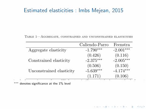
Table 1—Aggregate, constrained and unconstrained elasticities
Caliendo-Parro FeenstraAggregate elasticity -1.790∗∗∗ -2.001∗∗∗
(0.426) (0.116)Constrained elasticity -2.375∗∗∗ -2.005∗∗∗
(0.506) (0.150)Unconstrained elasticity -5.639∗∗∗ -4.174∗∗∗
(1.171) (0.106)Note: Standard errors in parentheses, ∗∗∗ denotes significance at the 1 percent level. Import elastic-ity computed as ηj =
∑km
kj (1 − λkj )εkj , ηj = ε
∑km
kj (1 − λkj ) and ηj = ε
∑km
kj (1 − λkj ), in the
unconstrained, constrained and aggregate cases, respectively.
goods relative to domestic substitutes is not instrumented. Inasmuch as the priceof domestic goods falls in response to the threat of foreign competition, thiscreates an attenuating endogeneity bias, which can explain such low values. Thetwo estimators used in this paper were designed to alleviate such endogeneity.27
C. Aggregate and Constrained Estimates
Table 1 reports the values of the trade elasticity in response to a macroeconomicshock, as implied by either the gravity approach, or by Feenstra’s estimation. Foreither approach, the table first reports the macroeconomic elasticity implied byaggregate data, ε
∑km
kj (1− λkj ), then its value implied by pooled sectoral data,
ε∑
kmkj (1 − λkj ), and finally its value implied by heterogeneous sectoral data,∑
kmkj (1− λkj )εk.
In aggregate data, the macroeconomic trade elasticity is −1.79 using the gravityestimation, and −2.00 using Feenstra’s estimation. The point estimates are notsignificantly different from each other. They are not significantly different eitherfrom conventional estimates obtained on aggregate data. For instance, they arewithin the range reported in Francis, Schumacher and Stern (1976), or in Gold-stein and Kahn (1985). For US aggregate trade, the latter report a range of −1.03to −1.76. In the words of Backus, Kehoe and Kydland (1994): “The most reliablestudies seem to indicate that for the United States the elasticity [of substitution]is between 1 and 2” (p.91). This corresponds to an aggregate import elasticityaround −1.
Are there elasticity estimates that are high in aggregate data? Eaton andKortum (2002) identify the aggregate trade elasticity that, in a Ricardian trademodel, maps into the international distribution of productivity. They find ε =
27Table 5 in Head and Mayer (2014) reports similar results: In a meta-analysis of gravity regressionswhere changes in the relative price of imports are captured with tariffs, the median trade elasticity is−5.09. But it is −1.12 if import prices are measured with exchange rate movements, wage differences,or with directly observed (and non-instrumented) changes in import prices.
∗∗∗ denotes significance at the 1% level

Estimated elasticities : Imbs Mejean, 2015
• Heterogeneity bias is substantial and matters quantitatively
• Models calibrated with heterogeneity-consistent elasticities are betterable to reproduce the behaviour of a multi-sector model
• Show this is the case of a standard IRBS model (Backus, et al, 1994)and a strandard trade model (Arkolakis et al, 2012)
• Might explain the “International Elasticity Puzzle”
Other source of aggregation issues
• Short-run / Long-run Elasticities
• Macro literature typically distinguishes between short-run andlong-run elasticities using time-series analysis
• Ruhl (2008) : Difference bw SR/LR elasticities might come from theresponse at the extensive margin to temporary/permanent shocks
• Permanent shocks (eg tariff) are more likely to induce extensiveadjustments
• Might explain discrepancies between elasticities estimated in macro(identification in the time-series using ER shocks) versus in trade(identification in the cross-section using tariff shocks)
• Heterogeneous firms
• Same argument as before
• Pooling across firms might induce an heterogeneity bias if the size offirms is systematically correlated with the trade elasticity (whichseems to be the case, Berman et al, 2011)
SR/LR elasticities : Ruhl, 2008
• Model of business cycle fluctuations with
• Entry cost of exporting and heterogeneous firms (Melitz, 2003)
• Aggregate TFP shocks (BKK, 1994)
⇒ Endogenous export participation based on expected future value ofexporting
• Extensive adjustments more pronounced after permanent shocksthan after temporary shocks
• In the SR, ie before extensive adjustments take place, trade elasticityis small / In the LR, trade elasticity is large for large enough /permanent shocks
SR/LR elasticities : Ruhl, 2008
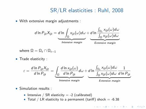
• With extensive margin adjustments :
d lnPijtXijt = d ln
∫
Ω
xijt(ω)dω
︸ ︷︷ ︸Intensive margin
+ d ln
∫Ωt
xijt(ω)dω∫Ωxijt(ω)dω
︸ ︷︷ ︸Extensive margin
where Ω = Ωt ∩ Ωt−1
• Trade elasticity :
ε =d lnPijtXijt
d lnPijt=
∫
Ω
d ln xijt(ω)
d lnPijtdω
︸ ︷︷ ︸Intensive margin
+ d ln
∫Ωt
xijt(ω)dω∫Ωxijt(ω)dω
1
d lnPijt︸ ︷︷ ︸Extensive margin
• Simulation results :
• Intensive / SR elasticity = -2 (calibrated)• Total / LR elasticity to a permanent (tariff) shock = -6.38
Firm heterogeneity : BMM, 2011
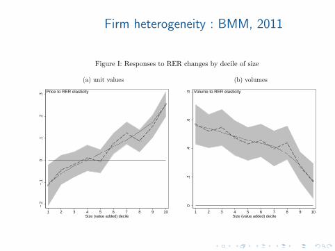
Figure I: Responses to RER changes by decile of size
(a) unit values (b) volumes
−.2
−.1
0.1
.2.3
1 2 3 4 5 6 7 8 9 10Size (value added) decile
Price to RER elasticity
0.2
.4.6
.8
1 2 3 4 5 6 7 8 9 10Size (value added) decile
Volume to RER elasticity
number of destination. Pricing-to-market increases with counts of destinations (panel a) which implies
that the elasticity of exports to exchange rate movements falls with this measure of performance (panel
b).27
Finally, Table A.1 in the appendix shows that the heterogeneous response of exports to exchange rate
movements is also observed at the sectoral level: an increase in the average productivity of the sector
(where a sector is defined at the NES114 level - 114 sectors) dampens the elasticity of export values to
exchange rate. In columns (1) and (2) we use the total value of exports, computed by destination and
sector, as the dependent variable. Columns (3) and (4) considers only the intensive margin, i.e. the
value of exports of firms that were already exporters in t − 1 (continuing exporters). In both cases, the
coefficients on the interaction of sectoral TFP (mean or median) with the real exchange rate exchange
rate is negative and highly significant.
Alternatives. We now consider three explanations, alternative to our mechanism, which can explain
the heterogenous response to exchange rate movements.28
(i) Imported Inputs. If the share of imported inputs in production is higher for high performance firms,
a depreciation of the euro may increase more their marginal cost of production through increased import
27Figure W.3 in the online appendix shows the results when using 10 bins of number of destinations instead of 20.28Note that all the results of this section are robust to the inclusion of all firms (main product sample) and to the use
of two alternative performance indicators, value added per worker and number of employees (see Table W.7 to W.9 in theonline appendix).
18
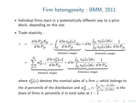
Firm heterogeneity : BMM, 2011
• Individual firms react in a systematically different way to a priceshock, depending on this size
• Trade elasticity :
ε =d lnPijtXijt
d lnPijt=
∫
Ω
d ln xijt(ω)
d lnPijtdω
︸ ︷︷ ︸Intensive margin
+ d ln
∫Ωt
xijt(ω)dω∫Ωxijt(ω)dω
1
d lnPijt︸ ︷︷ ︸Extensive margin
=D∑
d=1
wdijt−1
d ln xdijt(ω)
d lnPijt
︸ ︷︷ ︸Intensive margin
+ d ln
∫Ωt
xijt(ω)dω∫Ωxijt(ω)dω
1
d lnPijt︸ ︷︷ ︸Extensive margin
where xdijt(ω) denotes the nominal sales of a firm ω which belongs to
the d-percentile of the distribution and wdijt−1 ≡
∫Ωd
xijt−1(ω)dω∫Ωxijt−1(ω)dω
is the
share of firms in percentile d in total sales at t − 1

Firm heterogeneity : BMM, 2011
• IV strategy implies :
d ln xdijt(ω)
d lnPijt= 1− εd = 1− εdx
εdp − 1
where εdx ≡d ln X d
fjt
d ln RERjtand εdp ≡
d ln Pdfjt
d ln RERjt
• Estimation results suggest εd increasing in d (quantities lessresponsive to prices for large firms) because
• quantities are less responsive to ER (εdx decreasing in d)
• prices are more responsive to ER (εdp increasing in d)
• Since large firms account for a disproportionate share of aggregateexports, aggregate elasticities are driven down by large firms

Conclusion
• Trade elasticity is the key variable in international economics whichdetermines :
• The welfare gains from trade
• The transmission of shocks across countries (expenditure switchingeffect)
• ...
• Given the importance, it is surprising that so little is known about itsvalue and variability across countries / sectors / time / etc.

References- Amiti, Itskhoki & Konings, 2016, “International Shocks and Domestic
Prices : How Large are Strategic Complementarities ?”, NBER WorkingPaper, 22119
- Arkolakis, Costinot & Rodriguez-Clare, 2012, “New Trade Models, SameOld Gains ?”, American Economic Review, 102(1) :94-130
- Backus, Kehoe, & Kydland, 1994. “Dynamics of the Trade Balance andthe Terms of Trade : The J-Curve ?,” American Economic Review,84(1) :84-103
- Berman, Martin & Mayer, 2011, “How do Different Exporters React toExchange Rate Changes ?”, Quarterly Journal of Economics127(1) :437-4493
- Caliendo & Parro, 2015. “Estimates of the Trade and Welfare Effects ofNAFTA,” Review of Economic Studies, 82(1) :1-44.
- Feenstra, 1994, “New Product Varieties and the Measurement ofInternational Prices.” American Economic Review, 84(1) :157–177
- Feenstra, Luck, Obstfeld & Russ, 2014. “In Search of the ArmingtonElasticity,” NBER Working Papers 20063
- Fitzgerald & Haller, 2014. “Exporters and Shocks : Dissecting theInternational Elasticity Puzzle,” NBER Working Papers 19968

- Head & Mayer, 2014, “Gravity Equations : Workhorse,Toolkit, andCookbook”, in Gopinath, Helpman and Rogoff (eds), Handbook ofInternational Economics, vol.4 :131–195
- Head & Ries, 2001. “Increasing Returns versus National ProductDifferentiation as an Explanation for the Pattern of U.S.-Canada Trade,”American Economic Review, 91(4) :858-876
- Hooper, Johnson & Marquez, 2000, “Trade Elasticities for G-7Countries,” Princeton Studies in International Economics 87
- Imbs & Mejean, 2015. “Elasticity Optimism,” American EconomicJournal : Macroeconomics, 7(3) :43-83
- Krugman, 1987. “Pricing to market when the exchange rate changes”. In :Arndt, Richardson (Eds.), Real-Financial Linkages among OpenEconomies. MIT Press
- Novy, 2013. “International trade without CES : Estimating transloggravity,” Journal of International Economics, 89(2) :271-282
- Orcutt, 1950, “Measurement of Price Elasticities in International Trade,”The Review of Economics and Statistics, 32(2) : 117–132
- Ruhl, 2008, “The International Elasticity Puzzle”, mimeo

![C5.2 Elasticity and Plasticity [1cm] Lecture 2 Equations ...](https://static.fdocument.org/doc/165x107/622f8f3994946046a5727b7b/c52-elasticity-and-plasticity-1cm-lecture-2-equations-.jpg)