Tracker

2

Tracker Functions

•  Charged particle trajectory •  Momentum measurement

•  Requires magnetic field •  Primary and secondary vertex determination •  Particle ID (in conjunction with other detectors):

•  e/γ discrimination •  Electron ID using transition radiation •  p/K/π separation using dE/dx vs p •  p/K/π separation in combination with Cerenkov angle

•  Integral part of energy flow measurement •  Trigger

3

Typical Tracking Detectors

•  Silicon •  Resolution ~ 10 µm (sometimes poorer to save cost) •  Very high granularity possible •  Expensive •  Small number of layers, N ~ 10 (CMS: 3 pixel + 10 strip pairs)

•  Wire chamber •  Resolution ~ 100 µm transverse, (much) worse along wire •  Poor granularity •  Relatively cheap •  Many hit layers, N ~ 100 (UA1: ~70; CDF: 96)

•  Time projection chamber •  Resolution ~ 100+ µm (in 3D) •  Good granularity because of 3D •  Very long integration time

-  ALEPH: ~50 µsec; ALICE: ~90 µsec -  CEPC bunch crossing ~ 3 µsec

4

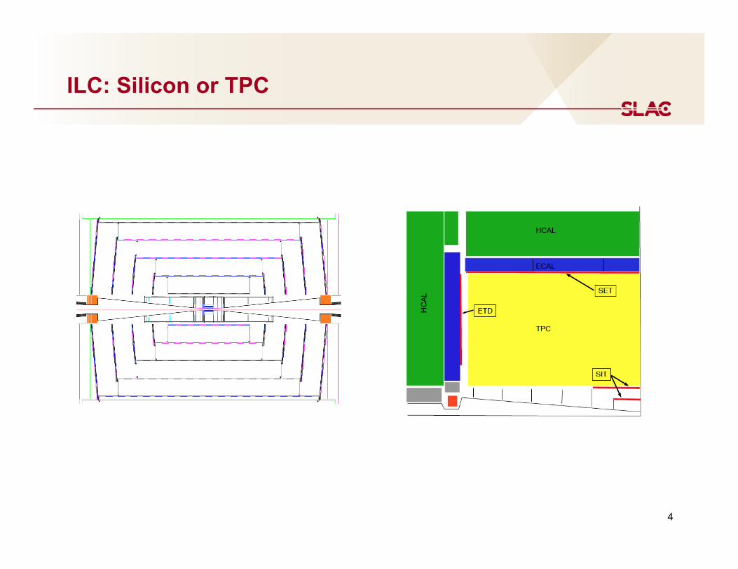
ILC: Silicon or TPC

Momentum Resolution

5

6

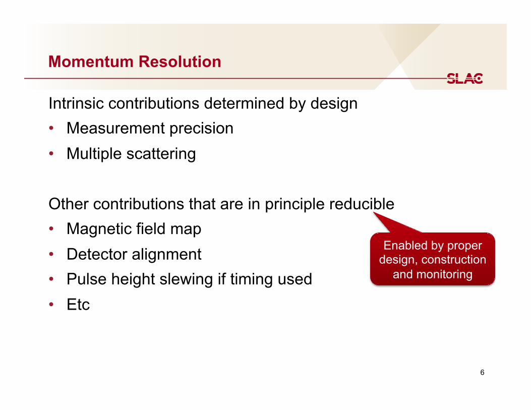
Momentum Resolution

Intrinsic contributions determined by design •  Measurement precision •  Multiple scattering Other contributions that are in principle reducible •  Magnetic field map •  Detector alignment •  Pulse height slewing if timing used •  Etc

Enabled by proper design, construction

and monitoring

7

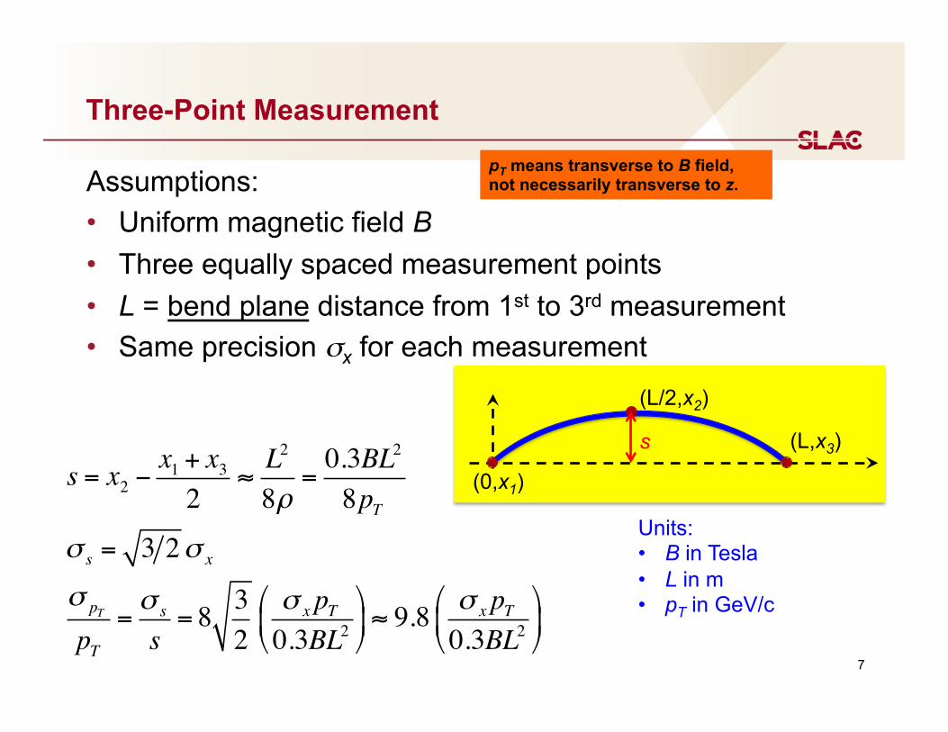
Three-Point Measurement

Assumptions: •  Uniform magnetic field B •  Three equally spaced measurement points •  L = bend plane distance from 1st to 3rd measurement •  Same precision σx for each measurement

(0,x1)

(L/2,x2)

(L,x3) s

s = x2 −x1 + x32

≈L2

8ρ=0.3BL2

8pTσ s = 3 2σ x

σ pT

pT=σ s

s= 8 3

2σ x pT0.3BL2#

$%

&

'( ≈ 9.8

σ x pT0.3BL2#

$%

&

'(

Units: •  B in Tesla •  L in m •  pT in GeV/c

pT means transverse to B field, not necessarily transverse to z.

8

Gluckstern Paper

•  Considers the general case of unequal spacing between hits and different precision among the hits.

•  Formulae for direction as well as momentum resolution. •  Incorporated into codes such as TRKERR and others •  Optimized (but not necessarily practical) layouts •  For best momentum resolution •  For best direction

9

N Equally Spaced Measurements with Fixed Precision

Assumptions: •  Uniform magnetic field B •  L = bend plane distance from 1st to Nth measurement •  Ignore multiple scattering, i.e. high-momentum limit

σ pT

pT≈

720N + 4

σ x pT0.3BL2"

#$

%

&' for large N

When you see (N+5) in some references, check

their definition of N!

10

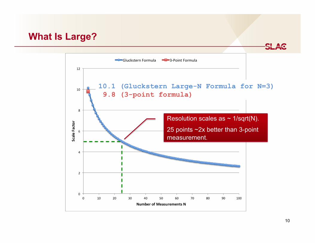
What Is Large?

10.1 (Gluckstern Large-N Formula for N=3) 9.8 (3-point formula)

Resolution scales as ~ 1/sqrt(N).

25 points ~2x better than 3-point measurement.

11

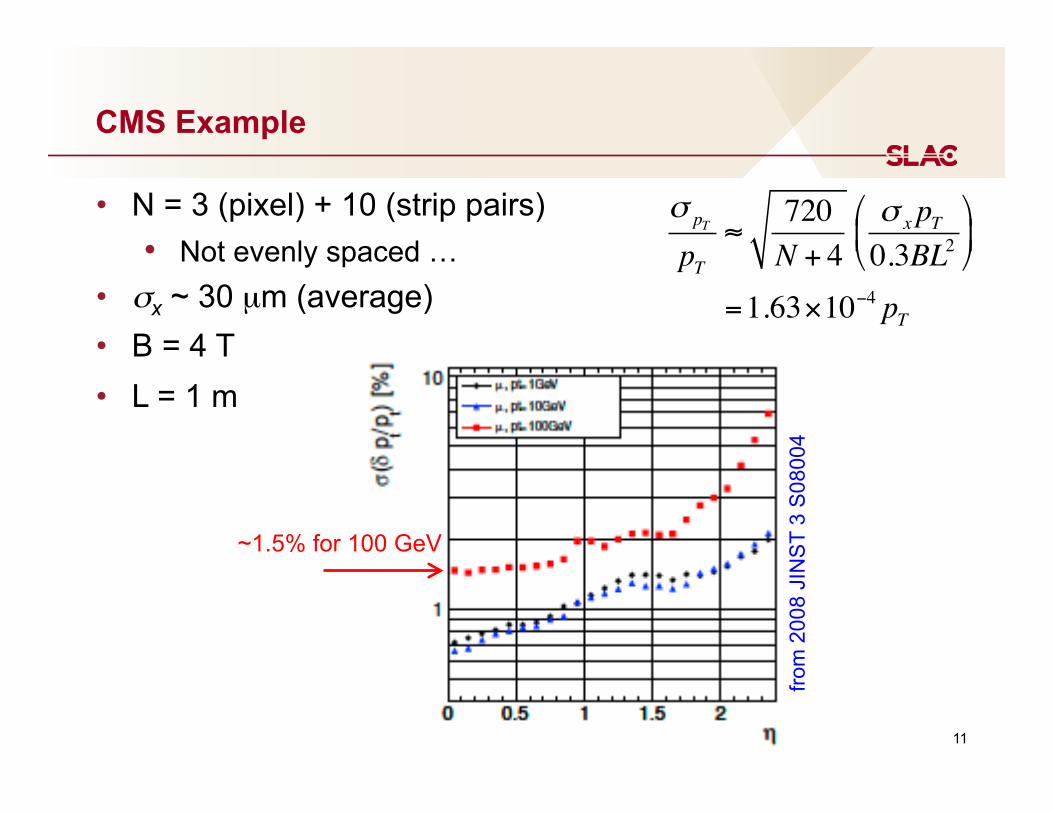
CMS Example

•  N = 3 (pixel) + 10 (strip pairs) •  Not evenly spaced …

•  σx ~ 30 µm (average) •  B = 4 T •  L = 1 m

σ pT

pT≈

720N + 4

σ x pT0.3BL2"

#$

%

&'

=1.63×10−4 pT

~1.5% for 100 GeV

from

200

8 JI

NS

T 3

S08

004

12

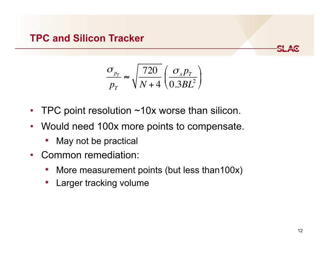
TPC and Silicon Tracker

•  TPC point resolution ~10x worse than silicon. •  Would need 100x more points to compensate.

•  May not be practical •  Common remediation:

•  More measurement points (but less than100x) •  Larger tracking volume

σ pT

pT≈

720N + 4

σ x pT0.3BL2"

#$

%

&'

13

Resolutions  are  well  estimated  using  Gluckstern  formula.    

Before  there  is  an  advanced  detector  design  including  realistic  supports  and  services,  detailed  simulation  can  be  misleading:  precision  achieved  beyond  Gluckstern  formula  is  compromised  by  inaccuracies  due  to  poorly  understood  material  inventory  etc.      

14

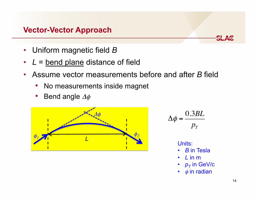
Vector-Vector Approach

•  Uniform magnetic field B •  L = bend plane distance of field •  Assume vector measurements before and after B field

•  No measurements inside magnet •  Bend angle Δφ

Δφ =

0.3BLpT

Units: •  B in Tesla •  L in m •  pT in GeV/c •  φ in radian

Δφ

L φ1 φ2

Multiple Scattering

15

16

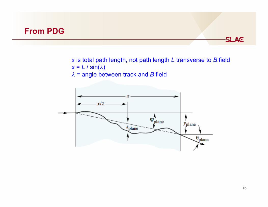
From PDG

x is total path length, not path length L transverse to B field x = L / sin(λ) λ = angle between track and B field

17

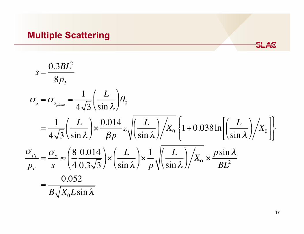
Multiple Scattering

s = 0.3BL2

8pT

σ s =σ splane=14 3

Lsinλ!

"#

$

%&θ0

=14 3

Lsinλ!

"#

$

%&×0.014β p

z Lsinλ!

"#

$

%& X0 1+ 0.038ln

Lsinλ!

"#

$

%& X0

(

)*

+

,-

./0

123

σ pT

pT=σ s

s≈840.0140.3 3

!

"#

$

%&×

Lsinλ!

"#

$

%&×1p

Lsinλ!

"#

$

%& X0 ×

psinλBL2

=0.052

B X0Lsinλ

Magnetic Field

18

19

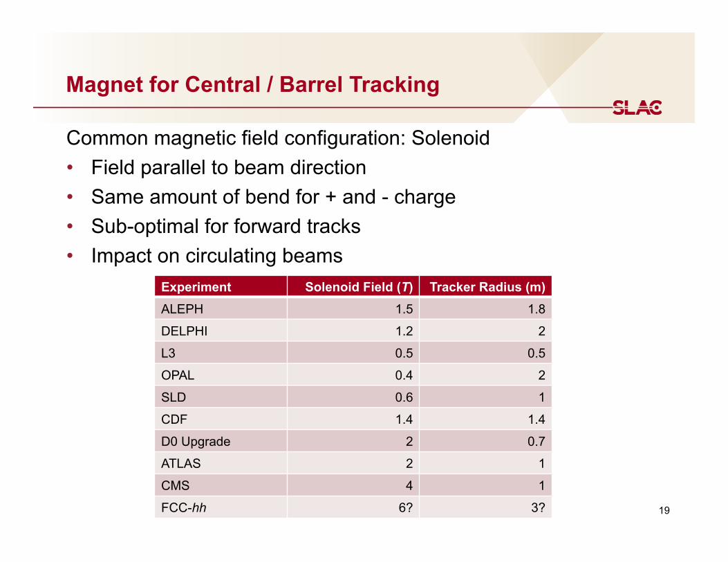
Magnet for Central / Barrel Tracking

Common magnetic field configuration: Solenoid •  Field parallel to beam direction •  Same amount of bend for + and - charge •  Sub-optimal for forward tracks •  Impact on circulating beams Experiment Solenoid Field (T) Tracker Radius (m)

ALEPH 1.5 1.8

DELPHI 1.2 2

L3 0.5 0.5

OPAL 0.4 2

SLD 0.6 1

CDF 1.4 1.4

D0 Upgrade 2 0.7

ATLAS 2 1

CMS 4 1

FCC-hh 6? 3?

UA1

20

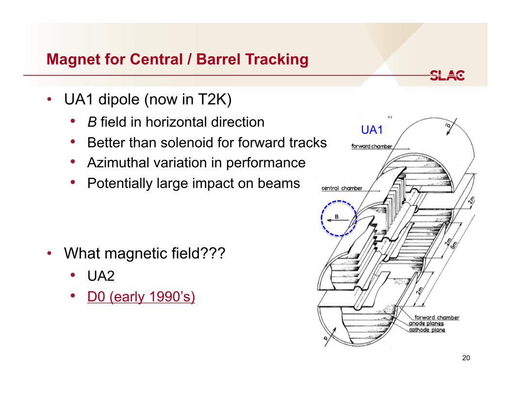
Magnet for Central / Barrel Tracking

•  UA1 dipole (now in T2K) •  B field in horizontal direction •  Better than solenoid for forward tracks •  Azimuthal variation in performance •  Potentially large impact on beams

•  What magnetic field??? •  UA2 •  D0 (early 1990’s)

21

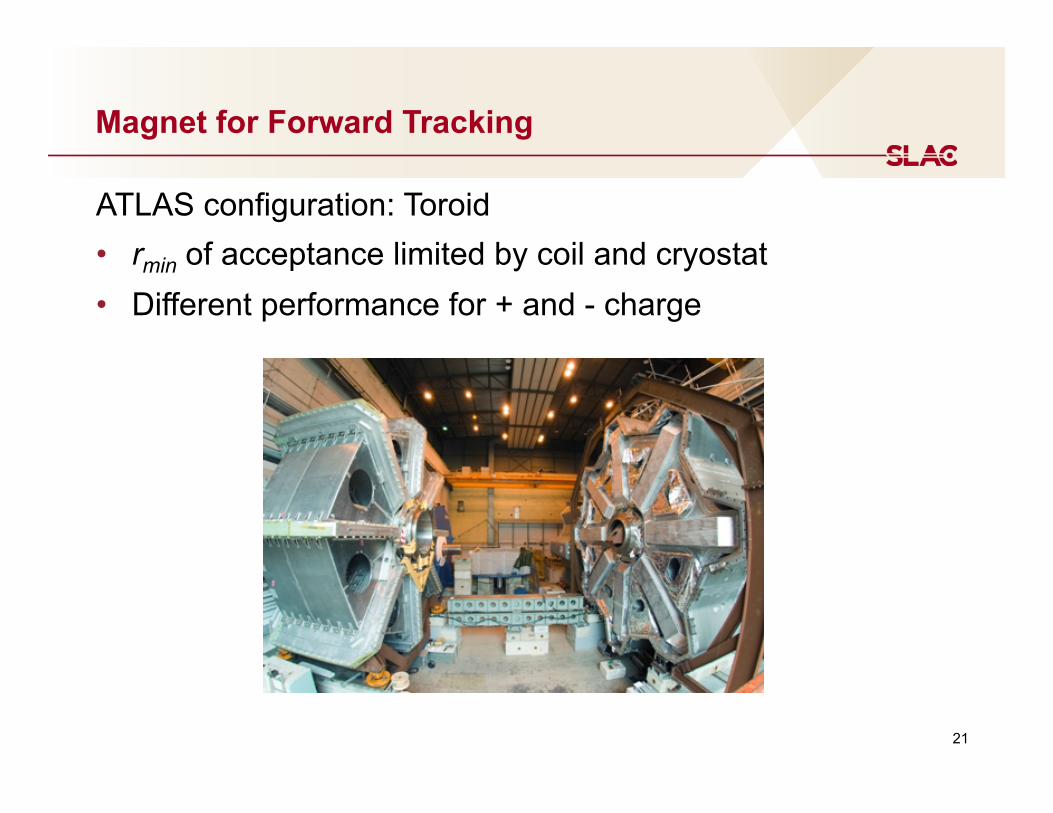
Magnet for Forward Tracking

ATLAS configuration: Toroid •  rmin of acceptance limited by coil and cryostat •  Different performance for + and - charge

22

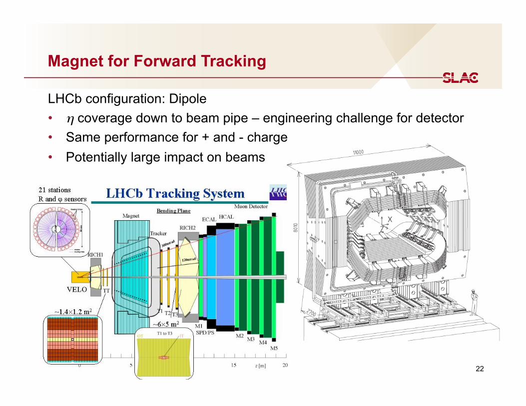
Magnet for Forward Tracking

LHCb configuration: Dipole •  η coverage down to beam pipe – engineering challenge for detector •  Same performance for + and - charge •  Potentially large impact on beams

23

Other Considerations

24

25

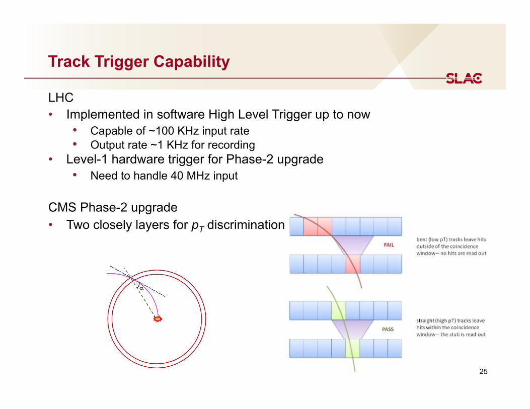
Track Trigger Capability

LHC •  Implemented in software High Level Trigger up to now

•  Capable of ~100 KHz input rate •  Output rate ~1 KHz for recording

•  Level-1 hardware trigger for Phase-2 upgrade •  Need to handle 40 MHz input

CMS Phase-2 upgrade •  Two closely layers for pT discrimination

26

Track Trigger Capability

Lepton collider •  Low rates so software implementation is sufficient •  How about FCC-ee (with crab waist) peak luminosity up

to ~ 9 x 1036 cm-2 sec-1

• 

from http://tlep.web.cern.ch/content/machine-parameters

27

Typical Approach to Pattern Recognition

•  Start with (small) subset of detector layers •  Select hits based on consistency with being a track

•  Subject to constraints as desired, such as IP pointing, minimum momentum and so on

•  Fit track •  Extrapolate / interpolate to other detector layers •  Attach additional hits and iterate

28

TPC and Silicon Tracker

Figure from a person working on ILD detector concept

29

Why It Is Important to Consider (in Early Design Stage)

•  Number of track candidates driven by all possible combinations of hits

•  Number of combinations scales as high power of Nhit •  Rapid increase at high hit rates •  Sensitive to hard-to-predict background rates •  Can be exacerbated by ill-conceived design

•  All track candidates, accepted or discarded, are computationally expensive

•  No easy fix once detector has been designed

30

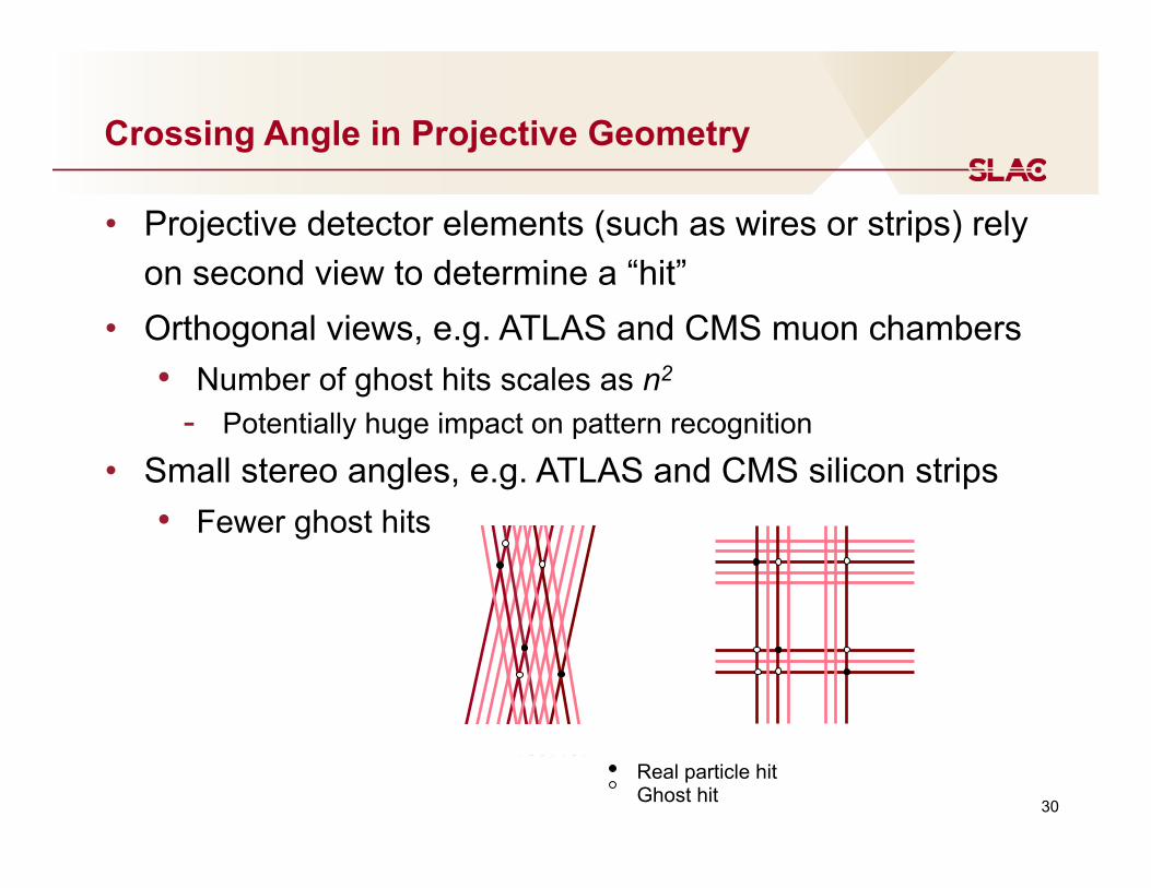
Crossing Angle in Projective Geometry

•  Projective detector elements (such as wires or strips) rely on second view to determine a “hit”

•  Orthogonal views, e.g. ATLAS and CMS muon chambers •  Number of ghost hits scales as n2

-  Potentially huge impact on pattern recognition

•  Small stereo angles, e.g. ATLAS and CMS silicon strips •  Fewer ghost hits

Real particle hit Ghost hit

31

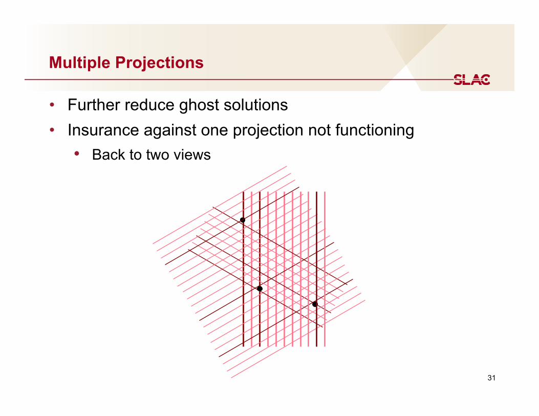
Multiple Projections

•  Further reduce ghost solutions •  Insurance against one projection not functioning

•  Back to two views

32

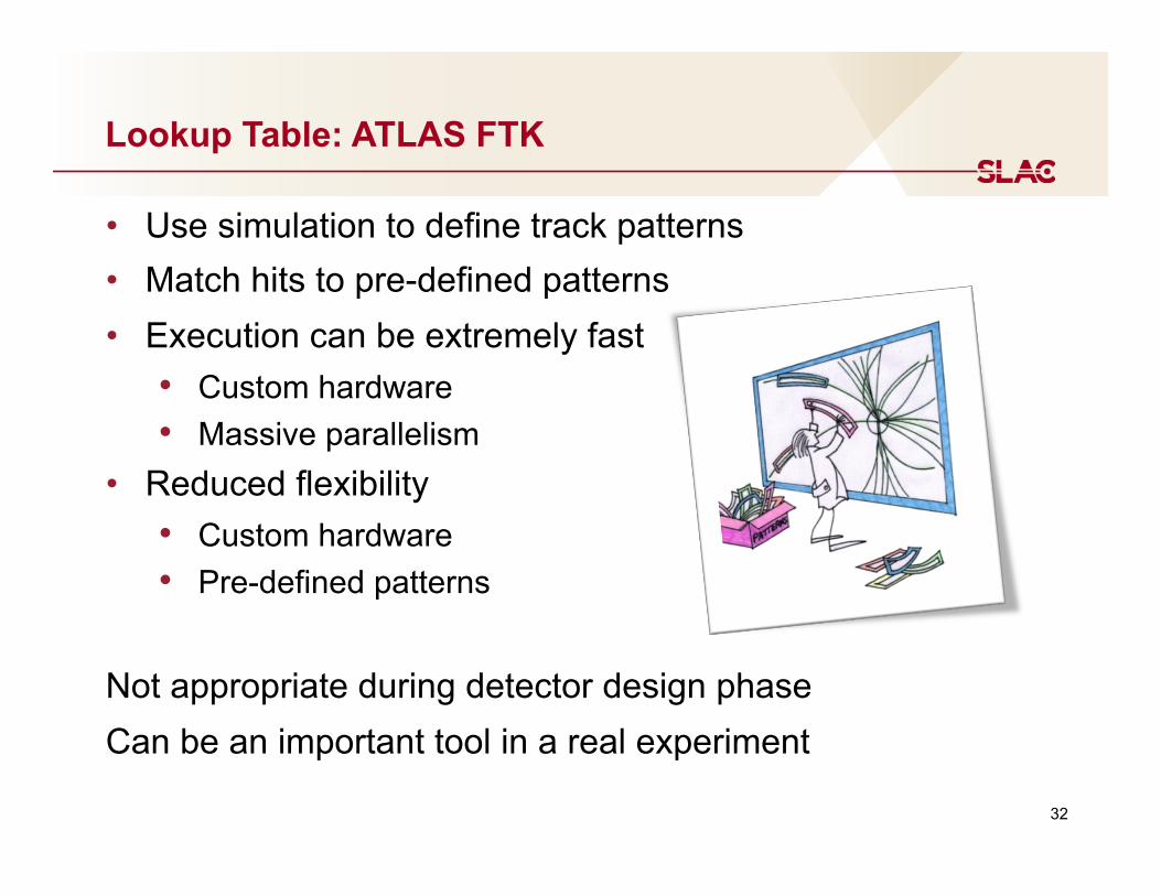
Lookup Table: ATLAS FTK

•  Use simulation to define track patterns •  Match hits to pre-defined patterns •  Execution can be extremely fast

•  Custom hardware •  Massive parallelism

•  Reduced flexibility •  Custom hardware •  Pre-defined patterns

Not appropriate during detector design phase Can be an important tool in a real experiment

33

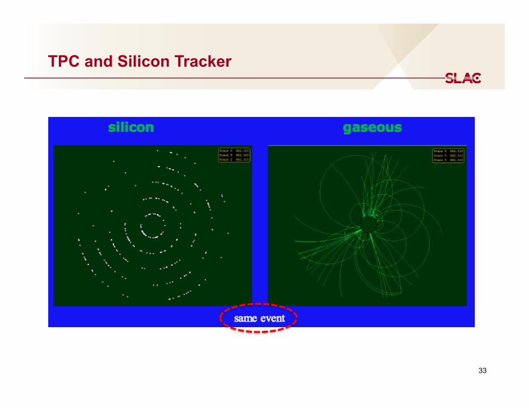
TPC and Silicon Tracker

Figure from a person working on ILD detector concept

34

Pattern Recognition in TPC and Silicon Tracker

Unfair visual comparison because •  3D in reality vs 2D in picture •  Measurement resolution much better than picture

granularity •  Algorithms much better than your eyes •  CMS provides existence proof that silicon trackers can

work, even in dense hit environments

Still, TPC-like tracker •  Pattern recognition likely to be simpler / more robust •  More efficient for short tracks

35

Silicon Tracker Alignment

•  Many independent modules with typical size (1-2 cm)2

•  Large number of degrees of freedom •  Hierarchy of structures, e.g.

•  Tracker made up of cylindrical layers •  Each layer made up of staves •  Each stave made up of modules

•  If these structures are well constructed and well understood, constraints can be applied to reduce number of degrees of freedom •  Less special alignment data needed •  Faster algorithmic convergence •  Avoid false minimums

36

Examples from Silicon Tracker Alignment

ATLAS IBL stave bowing •  Supposed to be free to slide on one end under differential

thermal expansion / contraction •  Actual behavior now understood in measurements on

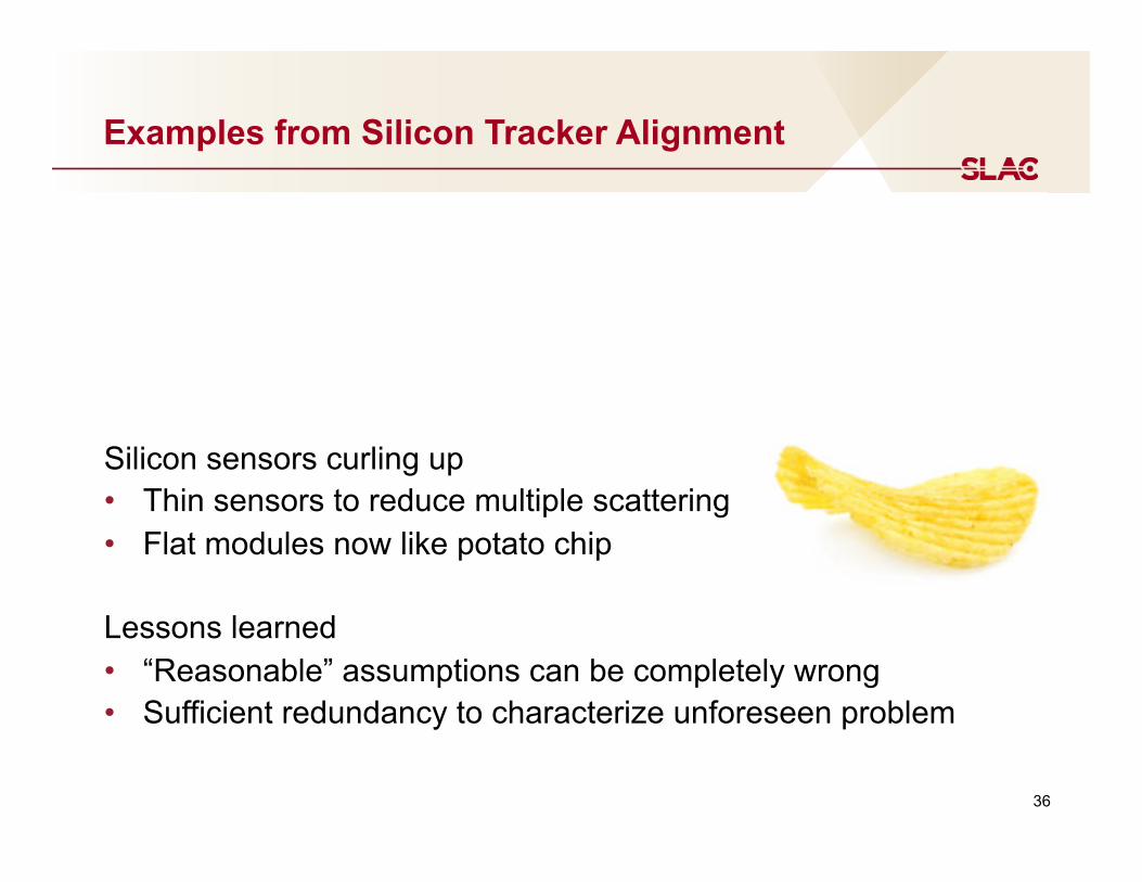
mock-ups and FEA calculations Silicon sensors curling up •  Thin sensors to reduce multiple scattering •  Flat modules now like potato chip

Lessons learned •  “Reasonable” assumptions can be completely wrong •  Sufficient redundancy to characterize unforeseen problem

37

TPC Field Distortion

Two sources of ions in TPC •  From tracks traversing TPC volume •  From avalanche in signal amplification region

•  Minimized with good design Ions drift very slowly to central electrode Distorting TPC drift field for subsequent tracks Elaborate alignment and calibration become an essential part of the TPC design.

38

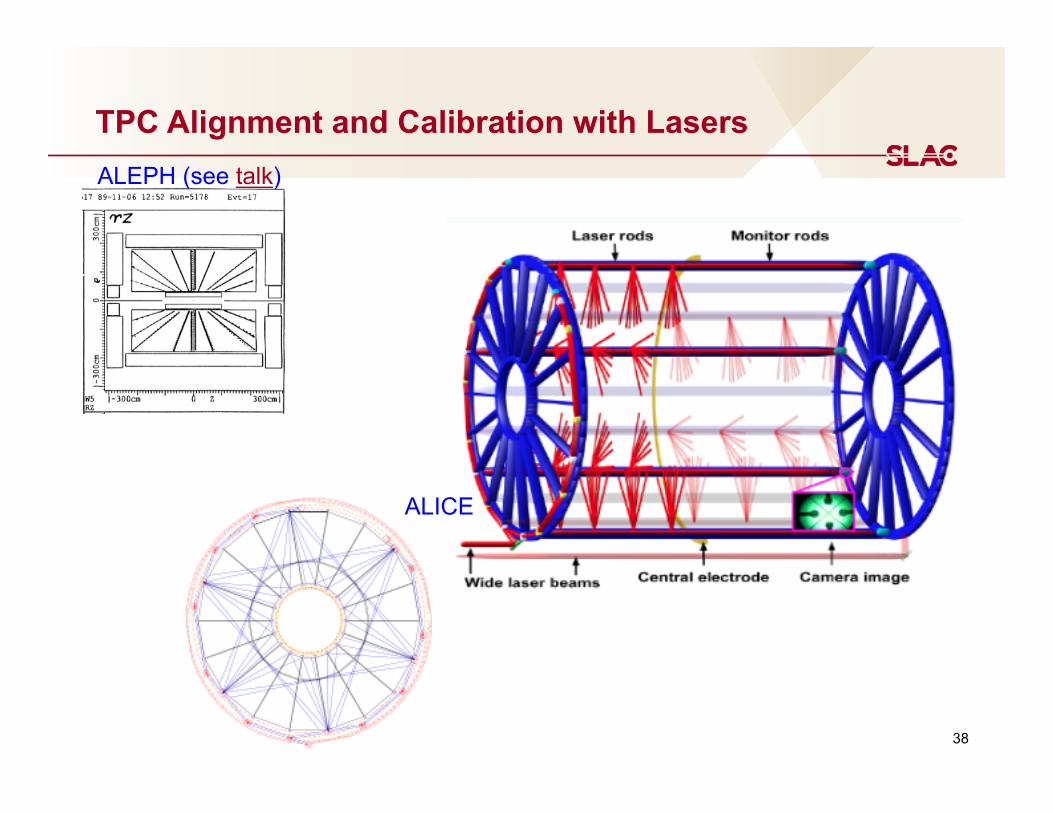
TPC Alignment and Calibration with Lasers ALEPH (see talk)

ALICE

39

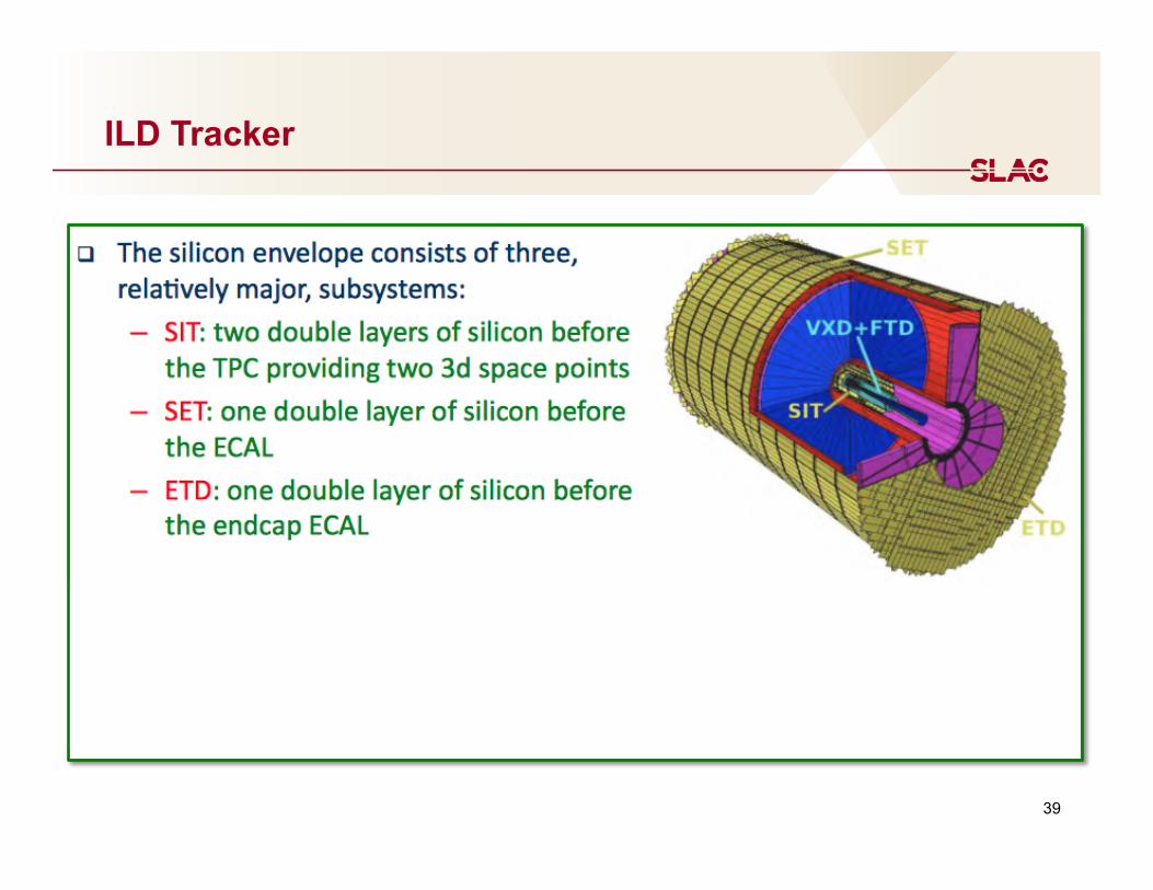
ILD Tracker

40

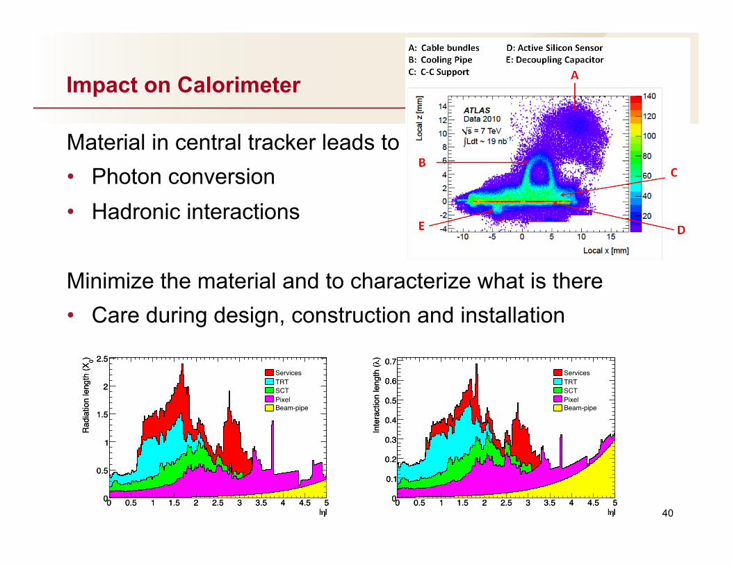
Impact on Calorimeter

Material in central tracker leads to •  Photon conversion •  Hadronic interactions Minimize the material and to characterize what is there •  Care during design, construction and installation

|η|0 0.5 1 1.5 2 2.5 3 3.5 4 4.5 5

) 0R

adia

tion

leng

th (X

0

0.5

1

1.5

2

2.5

|η|0 0.5 1 1.5 2 2.5 3 3.5 4 4.5 5

) 0R

adia

tion

leng

th (X

0

0.5

1

1.5

2

2.5ServicesTRTSCTPixelBeam-pipe

|η|0 0.5 1 1.5 2 2.5 3 3.5 4 4.5 5

)λ

Inte

ract

ion

leng

th (

0

0.1

0.2

0.3

0.4

0.5

0.6

0.7

|η|0 0.5 1 1.5 2 2.5 3 3.5 4 4.5 5

)λ

Inte

ract

ion

leng

th (

0

0.1

0.2

0.3

0.4

0.5

0.6

0.7ServicesTRTSCTPixelBeam-pipe

41

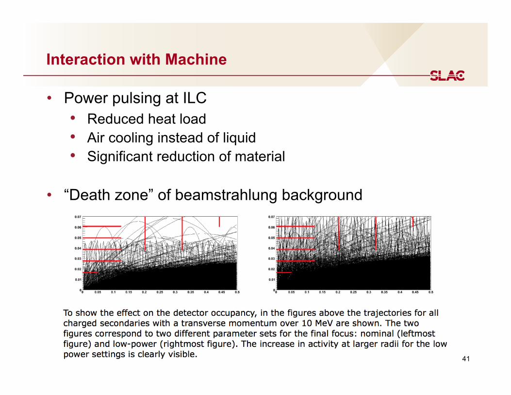
Interaction with Machine

•  Power pulsing at ILC •  Reduced heat load •  Air cooling instead of liquid •  Significant reduction of material

•  “Death zone” of beamstrahlung background

42

Summary

•  Easy and reliable resolution from Gluckstern formula •  Detailed simulation when there is well developed design •  Pay attention to the many things that can wreck a good-

on-paper design, e.g. •  Material, including services •  Detector stability and alignment •  Pattern recognition and other software implications •  Trigger capability as necessary •  Impact on other systems

Think about the whole experiment