Trace-minimal graphs and D-optimal weighing designsba70714/publications/tracemin.pdfTrace-minimal...

Trace-minimal graphs and D-optimal weighing designs

Bernardo M. Abrego

Silvia Fernandez-Merchant

Michael G. Neubauer

William Watkins

California State University, Northridge

March 23, 2004, v.115

Abstract

Let G(v, δ) be the set of all δ-regular graphs on v vertices. Certain graphs from among thosein G(v, δ) with maximum girth have a special property called trace-minimality. In particular, allstrongly regular graphs with no triangles and some cages are trace-minimal. These graphs play animportant role in the statistical theory of D-optimal weighing designs.

Each weighing design can be associated with a (0, 1)-matrix. Let Mm,n(0, 1) denote the set of allm× n (0,1)-matrices and let

G(m, n) = max{det XT X : X ∈ Mm,n(0, 1)}.

A matrix X ∈ Mm,n(0, 1) is a D-optimal design matrix if det XT X = G(m, n). In this paper weexhibit some new formulas for G(m, n) where n ≡ −1 (mod 4) and m is sufficiently large. Theseformulas depend on the congruence class of m (mod n). More precisely, let m = nt + r where0 ≤ r < n. For each pair n, r, there is a polynomial P (n, r, t) of degree n in t, which depends onlyon n, r, such that G(nt + r, n) = P (n, r, t) for all sufficiently large t. The polynomial P (n, r, t) iscomputed from the characteristic polynomial of the adjacency matrix of a trace-regular graph whosedegree of regularity and number of vertices depend only on n and r. We obtain explicit expressionsfor the polynomial P (n, r, t) for many pairs n, r. In particular we obtain formulas for G(nt + r, n)for n = 19, 23, and 27, all 0 ≤ r < n, and all sufficiently large t. And we obtain families of formulasfor P (n, r, t) from families of trace-minimal graphs including bipartite graphs obtained from finiteprojective planes, generalized quadrilaterals, and generalized hexagons.

Keywords: D-optimal weighing design, trace-minimal graph, regular graph, strongly regular graph,girth, cages, generalized polygonsAMS Subject Classification:Primary: 05C50, 62K05Secondary: 15A36, 05B25, 15A15, 05B20

1

March 23, 2004, v.115 2

1 Introduction

In [AFNW], the present authors established a relationship between certain regular graphs and D-optimaldesigns for weighing n ≡ −1 (mod 4) objects. We now further develop the graph-theoretic concept oftrace-minimality and use it to obtain additional results on D-optimality.

1.1 Trace-minimal graphs

Let G(v, δ) be the set of all δ-regular graphs on v vertices. We call G(v, δ) a graph class. Let A(G) be theadjacency matrix of a graph G. The characteristic polynomial of A(G) is denoted by ch(G, x) and thespectrum of A(G) is denoted by spec(A(G)). We also refer to ch(G, x) as the characteristic polynomialof the graph G and spec(A(G)) as the spectrum of G. Since A(G) is a symmetric (0, 1)-matrix with zeroson the diagonal and δ ones in each row, trA(G) = 0 and trA(G)2 = δv. These traces do not depend onthe structure of the graph G. However, for i ≥ 3, trA(G)i does depend on the structure of the graph.Indeed the (j, j) entry of A(G)i equals the number of closed walks of length i that start and end at vertexj. For G ∈ G(v, δ) define the trace sequence of G by TR(G) = (trA(G)3, trA(G)4, . . . , trA(G)n).

The trace sequence induces an order relation on the graphs in G(v, δ). Let G, H ∈ G(v, δ). We say G istrace-dominated by H if TR(G) is less than or equal to TR(H) in lexicographic order. In other words, G istrace-dominated by H if either trA(G)i = trA(H)i for all i (in which case spec(A(G)) = spec(A(H))) orthere exists a positive integer 3 ≤ k ≤ n such that trA(G)i = trA(H)i, for i < k and trA(G)k < trA(H)k.If G is trace-dominated by all graphs in G(v, δ), then we say that G is trace-minimal in G(v, δ). SinceG(v, δ) is finite, there always exist trace-minimal graphs in G(δ, v) and clearly they all have the samecharacteristic polynomial. Some graph classes G(v, δ), contain non-isomorphic graphs, each of which istrace-minimal. However, the smallest example known to us are two nonisomorphic cages in the graphclass G(70, 3). (See Sections 4.5 and 4.4.1.)

In addition to their application to the theory of D-optimal weighing designs, trace-minimal graphs areof independent interest. Indeed many well-known classes of regular graphs are trace-minimal includingstrongly regular graphs with no triangles, some cages, and the incidence graphs for various finite geome-tries. These and other families of trace-minimal graphs are given in Section 4. And it is clear from thedefinition that a trace-minimal graph G ∈ G(v, δ) must have maximum girth g among all graphs in itsgraph class G(v, δ). Furthermore, G must have the fewest number of g-cycles of any graph in the sameclass. We will describe more fully the connection between trace-minimality and girth in Section 2.

1.2 D-optimal weighing designs

Let Mm,n(0, 1) be the set of all m × n matrices all of whose entries are either 0 or 1. Removed fromits statistical setting, our problem is to determine, for each pair of positive integers m,n, the maximumvalue of the determinant of the n× n matrix XT X for X ∈ Mm,n(0, 1). If m < n then detXT X = 0, sowe will assume throughout that m ≥ n. Let

G(m,n) = max{detXT X : X ∈ Mm,n(0, 1)}.

A matrix X ∈ Mm,n(0, 1) is D-optimal if detXT X = G(m,n).

Statistical weighing designs date back to 1935 [Ya] and the 1940s [Ho] [Mo]. The goal is to estimatethe weights of n objects using a single-pan (spring) scale. (We do not assume that the scale is accurate,

March 23, 2004, v.115 3

its errors have a distribution.) Several objects are placed on the scale at once and their total weight isnoted. The information about which objects are place on the scale is encoded as a (0, 1)-n-tuple whosejth coordinate is 1 if object j is included in the weighing and 0 if not. (The weights of n objects cannot bereasonably estimated in fewer than n weighings, so the restriction m ≥ n makes statistical sense.) Withm weighings the corresponding (0, 1)-n-tuples form the rows of an m× n design matrix X ∈ Mm,n(0, 1).Certain design matrices give better estimates of the weights of the n objects than others. For example,under certain assumptions about the distribution of errors of the scale, D-optimal design matrices giveconfidence regions for the n-tuple of weights of the objects that have minimum volume. There are otherstandards for evaluating the efficiency of a design matrix such as A-optimality which corresponds to adesign matrix X for which tr(XT X)−1 is smallest. See [Pu] for an overview.

The problem also arises in a geometric settings. If X ∈ Mm,n(0, 1), the columns of X are vertices on theunit cube in Rm. The simplex spanned by the origin and each of the n columns of X has an n-dimensionalvolume equal to (1/n!)

√detXT X. So the problem of finding G(m,n) is equivalent to finding the volume

of the largest n-simplex on the vertices of the unit cube in Rm. See [HKL] for an up-to-date discussionand extensive list of references.

In general, the value of G(m,n) is not known. Although there are results for some pairs m,n, the onlyvalues of n for which G(m,n) is known for all m ≥ n are n = 1, 2, 3, 4, 5, 6. See [HKL] for n = 2, 3,[NWZ2] for n = 4, 5, and [NWZ3] for n = 6. Prior to this paper, the only values of n for which G(m,n)was known for all but a finite number of values of m (that is, for m sufficiently large) were n = 7, 11, 15.See [NW] for n = 7, and [AFNW] for n = 11, 15.

For example, the following formula for n = 7 was conjectured in [HKL]:

G(7t + r, 7) = 210(t + 1)rt7−r. (1)

In [NW], the formula was shown to be true for all t ≥ 15 and 0 ≤ r ≤ 6. In general, if n ≡ −1 (mod 4)and m = nt + r where 0 ≤ r < n, then G(m,n) is a polynomial P (n, r, t) in t of degree n which dependsonly on n and r. Indeed the authors of [AFNW] have shown that such a polynomial always exists. Tobe precise, we state the following theorem:

Theorem 1.1 [AFNW] For each n ≡ −1 (mod 4) and each 0 ≤ r < n, there exists a polynomialP (n, r, t) in t of degree n such that

G(nt + r, n) = P (n, r, t), (2)

for all sufficiently large t.

Thus for each pair n, r, we define the polynomial P (n, r, t) to be the one for which Equation (2) holdsfor all sufficiently large t. In some cases, this polynomial can be computed explicitly as in Equation (1).An explicit expression for the polynomial P (n, r, t) can be obtained from a trace-minimal graph from acertain graph class G(v, δ), where v and δ depend only on n, r. Thus in principle P (n, r, t) can be obtainedby comparing the trace sequences of all graphs in a graph class. The trace-minimal graphs for n = 7 and0 ≤ r < 7 are rather easy to find and all polynomials P (n, r, t) and their associated trace-minimal graphsfor n = 7, 11, 15 and all 0 ≤ r < n are exhibited in [AFNW].

In this paper we use trace-minimal graphs to obtain expressions for the polynomials P (n, r, t) for manynew pairs (n, r). In particular, we exhibit P (n, r, t) for n = 19, 23, and 27 and all 0 ≤ r < n. We presentthese and other new polynomials P (n, r, t) in Section 5. In Section 1.3 we describe the relationshipbetween trace-minimal graphs and the polynomials P (n, r, t). In Section 4 we exhibit several families of

March 23, 2004, v.115 4

trace-minimal graphs, some of which are associated with finite projective planes and other combinatorialconstructs. These graphs correspond to formulas for P (n, r, t) for infinite families of pairs (n, r) includingfamilies where r is large and small compared with n, and where r is near n/2.

Before going on, we should say that for some pairs n, r, where n ≡ −1 (mod 4), anomalies occur forsmall values of m. For example, let n = 7 and m = 18 so that t = 2 and r = 4. From Equation (1),G(7t+4, 7) = P (7, 4, t) for all sufficiently large t, where P (7, 4, t) = 4 28(t+1)4t3. Apparently t = 2 is notlarge enough. It is not hard to obtain an 18×7 design matrix A such that detAT A > P (7, 4, 2) = 663, 552.A simple computer program produced a design matrix such that detAT A = 684, 375. Thus G(18, 7) is atleast 684,375. We suspect that there are anomalies for all n ≥ 7, but the matter has not been investigated.

1.3 Trace-minimal graphs give expressions for P (n, r, t)

In this section we summarize the results in [AFNW] relating the polynomial P (n, r, t) to a trace-minimalgraph. Let n ≡ −1 (mod 4) so that n = 4p − 1 for some positive integer p. Let m = nt + r, where theremainder r satisfies 0 ≤ r < n. The formulas for P (n, r, t) from [AFNW] depend on the congruence classof r (mod 4). We begin with the cases r ≡ 1, 2 (mod 4):

Theorem 1.2 Let r = 4d + 1. Let G be a trace-minimal graph in G(2p, d). Then

P (n, r, t) =4(t + 1)[ch(G, pt + d)]2

t2. (3)

Theorem 1.3 Let r = 4d + 2. Let G be a trace-minimal graph in G(2p, p + d). Then

P (n, r, t) =4t[ch(G, pt + d)]2

(t− 1)2. (4)

To state the results for r ≡ −1, 0 (mod 4), we need to define a notion analogous to trace-minimalityfor bipartite graphs. Let B(2v, δ) be the set of all δ-regular bipartite graphs on 2v vertices and letB ∈ B(2v, δ). It follows from the regularity of B that each of the sets of vertices in the bipartition hascardinality v. Without loss of generality, we may assume that the sets of vertices in the bipartition are{1, 2, . . . , v} and {v + 1, v + 2, . . . , 2v}. Thus the adjacency matrix of B is of the form

A(B) =

[0 N(B)

N(B)T 0

],

where N(B) is a v × v (0, 1)-matrix having exactly δ ones in each row and each column.

It is clear that trA(B)i = 0 if i is odd and that trA(B)2j = 2tr((N(B)T N(B))j) otherwise. For j = 1,tr((N(B)T N(B)) = vδ, for all B ∈ B(2v, δ).

A graph B ∈ B(2v, δ) is bipartite-trace-minimal in B(2v, δ) if B is trace-dominated by all graphs inB(2v, δ). Clearly if G is trace-minimal in G(2v, δ) and bipartite, then it is bipartite-trace-minimal. Butsome bipartite-trace-minimal graphs are not trace-minimal.

March 23, 2004, v.115 5

Theorem 1.4 Let r = 4d−1. Suppose p/2 ≤ d < p. Let G be a trace-minimal graph in G(4p, 3p+d−1).Then

P (n, r, t) =4ch(G, pt + d− 1)

t− 3. (5)

Suppose 0 ≤ d < p/2. Let B be a bipartite-trace-minimal graph in B(4p, d). Then

P (n, r, t) =4(p(t− 1) + 2d)ch(B, pt + d)

t(pt + 2d). (6)

Theorem 1.5 Let r = 4d. Suppose 0 ≤ d ≤ p/2. Let G be a trace-minimal graph in G(4p, d). Then

P (n, r, t) =4ch(G, pt + d)

t. (7)

Suppose p/2 < d < p. Let B be a bipartite-trace-minimal graph on in B(4p, p + d). Then

P (n, r, t) =4(pt + 2d)ch(B, pt + d)(t− 1)(p(t + 1) + 2d)

. (8)

Equipped with these four theorems, one can translate the problem of finding an explicit expression ofP (n, r, t) for a given n ≡ −1 (mod 4) and remainder 0 ≤ r < n into the problem of finding an appropriatetrace-minimal or bipartite-trace-minimal graph. For example suppose n = 19 and r = 13 so that p = 5and r = 4d+1, where d = 3. This case falls within the scope of Theorem 1.2 and we seek a trace-minimalgraph in G(10, 3). The Petersen graph G, which is 3-regular on 10 vertices, is trace-minimal (see Section4.3). Since ch(G, x) = (x− 3)(x− 1)5(x + 2)4, Theorem 1.2 gives

P (19, 13, t) =4(t + 1)[ch(G, 5t + 3)]2

t2

= 20(5t + 2)10(5t + 5)9,

which proves one of the formulas in Theorem 5.21.

In a similar manner, we prove all of the theorems in Section 5 by exhibiting the required trace-minimaland bipartite-trace-minimal graphs and the corresponding characteristic polynomials. The proofs thateach graph is trace-minimal or bipartite-trace-minimal will be given later in Section 4.

2 Sufficient conditions for trace-minimality

All trace-minimal graphs G ∈ G(v, δ) have maximum girth in their graph class G(v, δ). And many ofthe graphs we catalog in Section 4 satisfy one of two conditions involving girth that are sufficient fortrace-minimality. Thus it is convenient to state these conditions before listing these families of graphs.

Let cyc(G, i) denote the number of cycles of length i in the graph G. This first condition for trace-minimality is the following:

Theorem 2.1 Let G be a graph with maximum girth g in G(v, δ). Suppose that for every graph H ∈G(v, δ), there exists an integer k ≤ 2g − 1 such that cyc(G, q) = cyc(H, q) for q < k and cyc(G, k) <cyc(H, k). Then G is trace-minimal in G(v, δ).

March 23, 2004, v.115 6

In particular, if G is the only graph in G(v, δ) with maximum girth g, then cyc(G, q) < cyc(H, q) for allq ≤ g and all H ∈ G(v, δ). Thus we have the following corollary:

Corollary 2.2 Let G be the only graph in G(v, δ) with maximum girth. Then G is the only trace-minimalgraph in G(v, δ).

The next condition involves the number of distinct eigenvalues in the spectrum (of the adjacency matrix)of G. Suppose a graph G has girth g and its adjacency matrix A(G) has k +1 distinct eigenvalues. Then[CDS, p88], the diameter D of G satisfies D ≤ k. It is clear that bg/2c ≤ D. Thus g ≤ 2k if the girth gis even and g ≤ 2k + 1 if g is odd. We analyze the case of equality in the next theorem.

Theorem 2.3 Let G be a connected regular graph with girth g and suppose that A(G) has k + 1 distincteigenvalues. If g is even then g ≤ 2k with equality only if G is trace-minimal. If g is odd then g ≤ 2k + 1with equality only if G is trace-minimal.

The proofs of these Theorems are in Section 7.

3 Graph definitions and notation

We begin with a list of some common graph notation that is used in this paper:

Iv the graph consisting of v independent vertices (no edges)Kv the complete graph on v verticesKv,v the complete bipartite graph with v vertices in each of the bipartition setsCv the cycle with v verticesvK2 a matching of v edges on 2v verticesK2v − vK2 the complete graph on 2v vertices with a matching of v edges removedKv,v − vK2 the complete bipartite graph with a matching of v edges removedGcomp the complement of a graph G

Bbcomp the bipartite-complement of a bipartite graph B (See 3.1.)G + H the direct sum of graphs G and H

kG the direct sum of k copies of G

G5H the join of graphs G and H (See 3.3.)G(l) the join of l copies of the graph G

3.1 Bipartite complement

Let B ∈ B(2v, δ) with adjacency matrix

A(B) =

[0 N(B)

N(B)T 0

].

March 23, 2004, v.115 7

The bipartite complement of B is the graph Bbcomp ∈ B(2v, v − δ) with adjacency matrix given by

A(Bbcomp) =

[0 J −N(B)

J −N(B)T 0

],

where J is the matrix all of whose entries are one. It is easy to see that trA(B)j = trA(Bbcomp)j = 0 ifj is odd and that

ch(Bbcomp, x)x2 − (v − δ)2

=ch(B, x)x2 − δ2

. (9)

So apart from the eigenvalues ±δ of A(B) and ±(v − δ) of Bbcomp, the spectra of B and Bbcomp are thesame. Thus

trA(Bbcomp)2j − 2(v − δ)2j = trA(B)2j − 2δ2j .

The next Lemma follows easily from that fact.

Lemma 3.1 If B is bipartite-trace-minimal in B(2v, δ), then Bbcomp is bipartite-trace-minimal inB(2v, v − δ).

3.2 Complement

The relationship between the characteristic polynomials of a graph G ∈ G(v, δ) and its complementGcomp ∈ G(v, δ′), where δ+δ′ = v−1, follows from A(G)+A(Gcomp) = J−I. Since we will need to computech(G, x) from ch(Gcomp, x), suppose that ch(Gcomp, x) = (x−δ′)p(x) Then ch(G, x) = ±(x−δ)p(−x−1),where the choice of plus-minus is made so that the polynomial is monic. More succinctly, the relationshipis:

ch(G, x)x− δ

= ±ch(Gcomp,−x− 1)x + v − δ

. (10)

3.3 Join

The join of two graphs Gi ∈ G(vi, δi) , i = 1, 2, is the graph on v = v1 + v2 vertices defined by

G 5 H = (Gcomp + Hcomp)comp. Then A(G 5 H) =

[A(G) J

J A(H)

]. The characteristic polynomial

of A(G1 5 G2) is related to the characteristic polynomials of A(G1) and A(G2) in the following way[CDS, FG]:

ch(G1 5G2, x)(x− δ1)(x− δ2)− v1v2

=ch(G1, x)ch(G2, x)(x− δ1)(x− δ2)

.

The join of two regular graphs is not regular unless v2 + δ1 = v1 + δ2 and in this case relationship of thecharacteristic polynomials is given by

ch(G1 5G2, x)(x− δ)(x + v − δ))

=ch(G1, x)ch(G2, x)(x− δ1)(x− δ2)

, (11)

where δ = v2 + δ1 = v1 + δ2. Furthermore the following Lemma holds:

Lemma 3.2 Let G1 ∈ G(v1, δ1) and G2 ∈ G(v2, δ2). If v2+δ1 = v1+δ2 = δ, then G15G2 ∈ G(v1+v2, δ).If G1 5G2 is trace-minimal then G1 and G2 are trace-minimal.

March 23, 2004, v.115 8

Proof: Let v = v1 + v2. Then,

trA(G1 5G2)j − δj − (δ − v)j = trA(G1)j − δj1 + trA(G2)j − δj

2.

It follows that if a graph H1 in G(v1, δ1) is trace-dominated by G1, then H1 5G2 is trace-dominated byG1 5 G2. So if G1 5 G2 is trace-minimal, then G1 is trace-minimal and, by a similar argument, G2 isalso trace-minimal.

4 Families of trace-minimal graphs

4.1 Graphs unique in their graph class

Each graph G in the next theorem is the only one in its graph class. Thus G is trace-minimal (bipartite-trace-minimal). The characteristic polynomials of the adjacency matrices for these graphs are well known.

Lemma 4.1 The following graphs are trace-minimal (bipartite-trace-minimal) in their graph class. Thecharacteristic polynomial is given:.

graph class G ch(G, x)G(v, 0) Iv xv

B(2v, 0) I2v x2v

G(v, v − 1) Kv (x− (v − 1))(x + 1)v−1

G(2v, 1) or B(2v, 1) vK2 (x− 1)v(x + 1)v

B(2v, v − 1) Kv,v − vK2 (x2 − (v − 1)2)(x2 − 1)v−1

B(2v, v) Kv,v (x− v)(x + v)x2v−2

G(2v, 2v − 2) K2v − vK2 = I(v)2 (x− 2v + 2)(x + 2)v−1xv.

4.2 Cycles and related graphs

Let Tchv(x) stand for the vth Tchebychev polynomial of the first kind, which is characterized by theidentity cos(vx) = Tchv(cos x). See [Ri] for details.

Lemma 4.2 The cycle graph G = Cv is the only trace-minimal graph in G(v, 2). Its characteristicpolynomial is:

ch(G, x) = 2Tchv(x/2)− 2.

The bipartite graph B = Kv,v − C2v = Cbcomp2v is the only bipartite-trace-minimal graph in B(2v, v − 2).

Its characteristic polynomial is:

ch(B, x) =(x2 − (v − 2)2)

x2 − 4(2Tch2v(x/2)− 2) .

Proof: The cycle Cv is the only graph in G(v, 2) with girth v, which is the maximal. Thus by Corollary2.2, Cv is trace-minimal.

The second part of the lemma follows from Lemma 3.1 and Equation (9).

March 23, 2004, v.115 9

4.3 Strongly regular graphs

A graph G on N vertices is strongly regular on the parameters (N, δ, λ, µ) if it is a δ-regular graph thatsatisfies the following two conditions:

(i) If u, v are vertices and (u, v) is an edge of G, then there are λ additional vertices that are joined toboth u and to v by an edge.

(ii) If u, v are vertices and (u, v) is not an edge of G, then there are µ vertices that are joined to both uand to v by an edge.

Lemma 4.3 Let G be a connected strongly δ-regular graph with no 3-cycles. Then G is trace-minimal.

This result follows immediately from Theorem 2.3. Every strongly regular graph G ∈ G(v, δ) has only3 = k + 1 distinct eigenvalues. Since there are no 3-cycles in G, the girth g of G must be at least 4. If gis odd, then 5 ≤ g ≤ 2k + 1 = 5. Hence g = 2k + 1 = 5. If g is even, then g = 2k = 4.

The following table lists all seven known strongly regular graphs G with parameter λ = 0 (no triangles)along with the girth and characteristic polynomial for A(G). (See [God]; see [CRC] for Higman-Sims(77).)

Name girth parameter set graph class characteristic polynomialC5 5 (5, 2, 0, 1) G(5, 2) (x− 2)(x2 + x− 1)2

Petersen 5 (10, 3, 0, 1) G(10, 3) (x− 3)(x− 1)5(x + 2)4

Clebsh 4 (16, 5, 0, 2) G(16, 5) (x− 5)(x− 1)10(x + 3)5

Hoffman-Singleton 5 (50, 7, 0, 1) G(50, 7) (x− 7)(x− 2)28(x + 3)21

Gewirtz 4 (56, 10, 0, 2) G(56, 10) (x− 10)(x− 2)35(x + 4)20

Higman-Sims (77) 4 (77, 16, 0, 4) G(77, 16) (x− 16)(x + 6)21(x− 2)55

Higman-Sims 4 (100, 22, 0, 6) G(100, 22) (x− 22)(x− 2)77(x + 8)22

4.4 Generalized polygons

Finite projective planes are one example of a class of geometries known as generalized polygons. (See[vM, p.5] for the definition and other details.) We are interested in generalized polygons of order q.Each line contains exactly q + 1 points and each point is on q + 1 lines. Generalized n-gons of order qwith n ≥ 3 exist if and only if n = 3, 4, 6 and they have been constructed whenever q is a power of aprime. Generalized 3-gons are projective planes, generalized 4-gons are called generalized quadrangles,and generalized 6-gons are called generalized hexagons.

The incidence graph [vM, p. 3] of a finite geometry Γ is the bipartite graph whose vertices are bipartitionedinto the lines and the points with an edge whenever a point and a line are incident. Thus the adjacencymatrix for the incidence graph G of a finite geometry is for the form

A(G) =

[0 N(G)

N(G)T 0

],

where N(G) is the line-point incidence matrix of Γ.

March 23, 2004, v.115 10

In the next three sections, we shall show that the spectrum of G has only n+1 distinct eigenvalues, fromwhich it follows by Theorem 2.3 that G is trace-minimal.

Theorem 4.4 Let G be the incidence graph for a generalized n-gon of order q. Then G is trace-minimal.

We need some facts about generalized n-gons.

Lemma 4.5 ([vM]) Let Γ be a generalized n-gon of order q and let G be the incidence graph of Γ. Then

The number of points and the number of lines in Γ is v = (qn − 1)/(q − 1).

Each line in Γ contains q + 1 points.

G ∈ B(2v, q + 1).

The girth of G is 2n.

In the next three sections, we compute the characteristic polynomials of the incidence graphs for projectiveplanes, generalized quadrangles, and generalized hexagons.

4.4.1 Projective planes

Let Γ be a finite projective plane of order q. (The parameter q is a power of a prime for all knownprojective planes.) There are v points and v lines, where v = (q3 − 1)/(q − 1). (See [vLW, p. 197].)Let d = q + 1 and r = 4d + 1 = 4q + 5. Let PP (q) ∈ G(2v, q + 1) be the incidence graph for Γ. ThenN(PP (q))T N(PP (q)) = qI + J , since each line contains q + 1 points and distinct lines intersect in onepoint. Similarly N(PP (q))N(PP (q))T = qI + J . The eigenvalues of qI + J are v + q = (q + 1)2 and q(v − 1 times). Thus ch(PP (q), x) = (x2 − (q + 1)2)(x2 − q)v−1 so A(PP (q)) has only four eigenvalues.The girth of PP (q) is 6. Thus by Theorem 2.3 PP (q) is trace-minimal. We have proved the followinglemma:

Lemma 4.6 Let PP (q) be the incidence graph of a projective plane of order q and let v = (q3−1)/(q−1).Then PP (q) is a trace-minimal graph in G(2v, q + 1) and

ch(PP (q), x) = (x2 − (q + 1)2)(x2 − q)v−1.

In general, projective planes of order q are not unique, that is not isomorphic as planes. Indeed there aretwo non-isomorphic projective planes of order q = 9, both of whose incidence graphs are trace-minimalin G(182, 10). One of them is the plane πF constructed from the field F with 9 elements. Another isπH , the Hughes plane. Not only are these planes nonisomorphic (as planes), but their incidence graphs,which are in G(182, 10), are nonisomorphic as graphs. This follows from the fact that πF contains a Fanoconfiguration whereas πH does not. Thus the graphs are not isomorphic since the Fano configurationinduces a subgraph of πH that is not present in πF . See [St, p.59] for definitions and details.

March 23, 2004, v.115 11

4.4.2 Generalized quadrangles

Let Γ be a generalized quadrangle of order q, where q is a power of a prime. There are v = (q4−1)/(q−1)points and lines in Γ. Let GQ(q) be the incidence graph of Γ. Then GQ(q) ∈ G(2v, q + 1). LetB = N(GQ(q))T N(GQ(q)), where N(GQ(q)) is the line-point incidence matrix for Γ. Using argumentssimilar to those in [vM, Appendix A], we get

Bi,j =

q + 1, if i = j

1, if i 6= j and points i and j are collinear0, else

.

Now let C = B − (q + 1)I so that Ci,j = 1 if points i, j are distinct and collinear and Ci,j = 0 otherwise.It follows from the properties of generalized quadrangles in [vM] that

(C2)i,j =

q(q + 1), if i = j

q − 1, if i 6= j and points i and j are collinearq + 1, else

.

It follows that C2 = (q +1)J +(q2−1)I−2C. Thus B2 = 2qB +(q +1)J . Since GQ(q) is (q +1)-regular,BJ = JB = (q + 1)2J . Thus B3 = 2qB2 + (q + 1)3J and (q + 1)2B2 = 2q(q + 1)2B + (q + 1)3J . Itfollows that B(B − 2qI)(B − (q + 1)2I) = 0. Thus B has at most three eigenvalues: 0, 2q, and (q + 1)2.We obtain the multiplicities, a, b, c, of these eigenvalues from the traces of B and B2 as follows:

a + b + c = q3 + q3 + q2 + q + 12qb + (q + 1)2c = trB = (q3 + q3 + q2 + q + 1)(q + 1)

(2q)2b + (q + 1)4c = trB2 = (q3 + q3 + q2 + q + 1)(q + 1)(2q + 1).

Solving for a, b, c, we obtain:

a = q(q2 + 1)/2, b = q(q + 1)2/2, c = 1. (12)

Since A(GQ(q))2 = N(GQ(q))T N(GQ(q))⊕N(GQ(q))N(GQ(q))T , we have proved the following lemma:

Lemma 4.7 Let GQ(q) be the incidence graph of a generalized quadrangle of order q and let v = (q4 −1)/(q − 1). Then GQ(q) is a trace-minimal graph in G(2v, q + 1) and

ch(GQ(q), x) = xq(q2+1)(x2 − 2q)q(q+1)2/2(x2 − (q + 1)2).

4.4.3 Generalized hexagons

Let Γ be a generalized hexagon of order q, where q is a power of a prime. There are v = (q6 − 1)/(q− 1)points and lines in Γ and 2v vertices in the incidence graph GH(q) of Γ. Let B = N(GH(q))T N(GH(q)),where N(GH(q)) is the line-point incidence matrix for Γ. Using arguments similar to those in [vM,Appendix A], we get

Bi,j =

q + 1, if i = j

1, if i 6= j and points i and j are collinear0, else.

March 23, 2004, v.115 12

Now let C = B − (q + 1)I so that Ci,j = 1 if points i, j are distinct and collinear and Ci,j = 0 otherwise.It follows from the properties of the generalized hexagons in [vM] that

(C2)i,j

=

q(q + 1), if i = j

q − 1, if points i and j are collinear1, if i, j are not collinear and not opposite0, if i, j are not collinear and opposite.

and

(C3)i,j

=

(q − 1)q(q + 1), if i = j

2(q + 1)q + (q − 1)(q − 2)− 1, if points i and j are collinear2(q − 1), if i, j are not collinear and not oppositeq + 1, if i, j are not collinear and opposite.

It follows thatC3 − (q − 3)C2 − (q + 1)J − (2q − 1)(q + 1)I = (2q2 + 2q − 3)C,

and soB3 − 4qB2 + 3q2B = (q + 1)J.

Since JB = BJ = (q + 1)2J , we get

B4 − 4qB3 + 3q2B2 = (q + 1)3J.

ThusB(B − 3qI)(B − qI)(B − (q + 1)2I) = 0.

Therefore B has at most four eigenvalues: 0, q, 3q, and (q + 1)2. The multiplicities, a, b, c, d of theseeigenvalues are computed from traces as follows:

a + b + c + d = v = q6−1q−1

qb + 3qc + (q + 1)2d = trB = q6−1q−1 (q + 1)

q2b + +9q2c + (q + 1)4d = trB2 = q6−1q−1 (q + 1)(2q + 1)

q3b + 27q3c + (q + 1)6d = trB3 = q6−1q−1 (q + 1)(5q2 + 4q + 1).

Solving for a, b, c, d we obtain

a = q(q2 + q + 1)(q2 − q + 1)/3b = q(q2 − q + 1)(q + 1)2/2c = q(q + 1)2(q2 + q + 1)/6d = 1.

(13)

Since the characteristic polynomial of A(GH(q)) is det(x2I −B), we have the following lemma:

Lemma 4.8 Let GH(q) be the incidence graph of a generalized hexagon of order q and let v = (q6 −1)/(q − 1). Then GH(q) is a trace-minimal graph in G(2v, q + 1) and

ch(GH(q), x) = x2a(x2 − q)b(x2 − 3q)c(x2 − (q + 1)2),

where a, b, c are given in Equation (13).

March 23, 2004, v.115 13

4.5 Cages

Let g, δ be positive integers. A cage is a δ-regular graph with girth g and a minimal number v(g, δ) ofvertices. It is clear from the definition of trace-minimality that if there is a cage in a graph class G(v, δ),that is there is a girth g such that v = v(g, δ), then every trace-minimal graph in G(v, δ) must be a cage.Thus we have the following lemma:

Lemma 4.9 If a graph class G(v, δ) contains a cage, then every trace-minimal graph in G(v, δ) is a cage.In particular, if G is the unique cage in G(v, δ), then G is trace-minimal.

There are only five known infinite families of cages: For any v, Kv (girth 3) and Kv,v (girth 4), for anyq power of prime PP (q) (girth 6), GQ(q) (girth 8), and GH(q) (girth 12). We have seen in previoussections that all of these graphs are trace-minimal. Apart from these infinite families, cages are knownfor only ten pairs of values (g, δ). In the next lemmas we list the trace-minimal graphs obtained fromthese pairs. Precise descriptions off all these graphs and information about their discoveries can be foundin [Gor].

Lemma 4.10 The following cages (g, δ) are unique in G(v(g, δ), δ). Thus they are trace-minimal.

Name g δ v(g, δ)Petersen 5 3 10Robertson 5 4 19O’Keefe-Wong 5 6 40Hoffman-Singleton 5 7 50O’Keefe-Wong 6 7 90McGee 7 3 24Balaban/McKay-Saager 11 3 112

The characteristic polynomials of the previous graphs are:

Name Characteristic PolynomialsPetersen (x− 3)(x− 1)5(x + 2)4

Robertson (x− 4)(x− 1)2(x2 − 3)2(x2 + x− 5)(x2 + x− 4)2(x2 + x− 3)2(x2 + x− 1)O’Keefe-Wong (5,6) (x− 6)(x− 2)18(x− 1)4(x + 2)5(x + 3)12

Hoffman-Singleton (x− 7)(x− 2)28(x + 3)21

O’Keefe-Wong (6,7) (x− 7)(x− 2)14(x + 2)14(x + 7)(x2 − 7)30

McGee (x− 3)(x− 2)3x3(x + 1)2(x + 2)(x2 + x− 4)(x3 + x2 − 4x− 2)4

Balaban/McKay-Myrvold (x− 3)x12(x2 − 6)15(x2 − 2)12(x3 − x2 − 4x + 2)2(x3 + x2 − 6x− 2)×(x4 − x3 − 6x2 + 4x + 4)4(x5 + x4 − 8x3 − 6x2 + 12x + 4)8

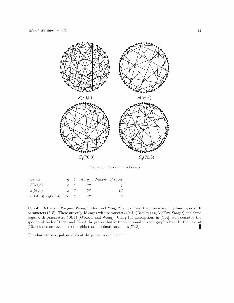
Lemma 4.11 The following cages (g, δ) are trace-minimal (see Figure 1).

March 23, 2004, v.115 14

S(30,5) S(58,3)

S1(70,3) S2(70,3)

Figure 1: Trace-minimal cages

Graph g δ v(g, δ) Number of cagesS(30, 5) 5 5 30 4S(58, 3) 9 3 58 18S1(70, 3), S2(70, 3) 10 3 70 3

Proof: Robertson,Wegner, Wong, Foster, and Yang, Zhang showed that there are only four cages withparameters (5, 5). There are only 18 cages with parameters (9, 3) (Brinkmann, McKay, Saager) and threecages with parameters (10, 3) (O’Keefe and Wong). Using the descriptions in [Gor], we calculated thespectra of each of them and found the graph that is trace-minimal in each graph class. In the case of(10, 3) there are two nonisomorphic trace-minimal cages in G(70, 3).

The characteristic polynomials of the previous graphs are:

March 23, 2004, v.115 15

Graph Characteristic PolynomialsS(30, 5) (x− 5)(x− 2)8(x + 1)(x + 3)4(x4 + 2x3 − 6x2 − 7x + 11)×

(x4 + 2x3 − 4x2 − 5x + 5)2

S(58, 3) (x− 3)(x− 1)(x + 2)(x4 − x3 − 4x2 + x + 2)(x5 + 3x4 − 5x3 − 17x2 + 9)×(x10 − 16x8 + x7 + 88x6 − 6x5 − 192x4 + 6x3 + 141x2 − 8x− 24)×(x18 − 25x16 + x15 + 254x14 − 17x13 − 1351x12 + 116x11 + 4054x10−427x9 − 6942x8 + 932x7 + 6607x6 − 1122x5 − 3209x4 + 654x3 + 626x2 − 136x− 13)2

S1(70, 3)S2(70, 3)

}(x− 3)(x− 1)4(x + 1)4(x + 3)(x2 − 6)(x2 − 2)(x4 − 6x2 + 2)5×(x4 − 6x2 + 3)4(x4 − 6x2 + 6)5

4.6 Sporadic trace-minimal graphs

Some trace-minimal graphs that do not fit into any of the previous categories are listed here along withthe graph class, characteristic polynomial. The notation for the sporadic trace-minimal graph in thegraph class G(v, δ) is S(v, δ) and for the bipartite-trace-minimal graph in B(2v, δ) is SB(2v, δ).

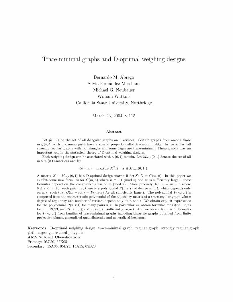
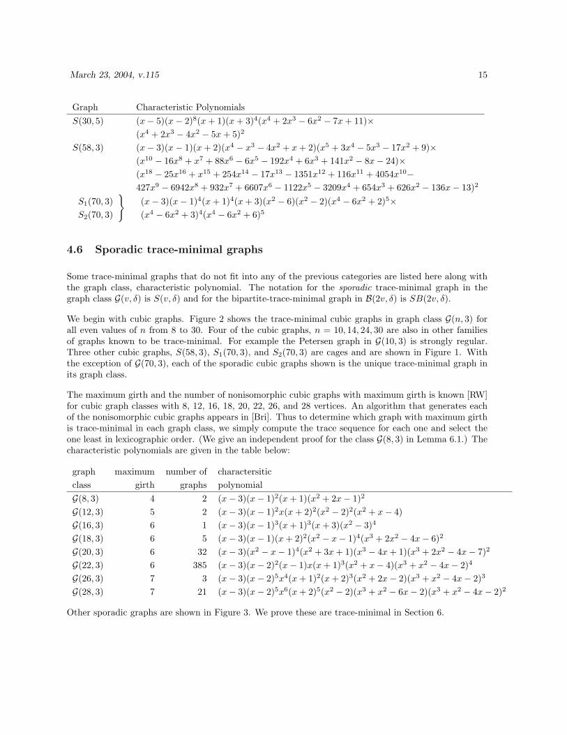
We begin with cubic graphs. Figure 2 shows the trace-minimal cubic graphs in graph class G(n, 3) forall even values of n from 8 to 30. Four of the cubic graphs, n = 10, 14, 24, 30 are also in other familiesof graphs known to be trace-minimal. For example the Petersen graph in G(10, 3) is strongly regular.Three other cubic graphs, S(58, 3), S1(70, 3), and S2(70, 3) are cages and are shown in Figure 1. Withthe exception of G(70, 3), each of the sporadic cubic graphs shown is the unique trace-minimal graph inits graph class.

The maximum girth and the number of nonisomorphic cubic graphs with maximum girth is known [RW]for cubic graph classes with 8, 12, 16, 18, 20, 22, 26, and 28 vertices. An algorithm that generates eachof the nonisomorphic cubic graphs appears in [Bri]. Thus to determine which graph with maximum girthis trace-minimal in each graph class, we simply compute the trace sequence for each one and select theone least in lexicographic order. (We give an independent proof for the class G(8, 3) in Lemma 6.1.) Thecharacteristic polynomials are given in the table below:

graph maximum number of charactersiticclass girth graphs polynomialG(8, 3) 4 2 (x− 3)(x− 1)2(x + 1)(x2 + 2x− 1)2

G(12, 3) 5 2 (x− 3)(x− 1)2x(x + 2)2(x2 − 2)2(x2 + x− 4)G(16, 3) 6 1 (x− 3)(x− 1)3(x + 1)3(x + 3)(x2 − 3)4

G(18, 3) 6 5 (x− 3)(x− 1)(x + 2)2(x2 − x− 1)4(x3 + 2x2 − 4x− 6)2

G(20, 3) 6 32 (x− 3)(x2 − x− 1)4(x2 + 3x + 1)(x3 − 4x + 1)(x3 + 2x2 − 4x− 7)2

G(22, 3) 6 385 (x− 3)(x− 2)2(x− 1)x(x + 1)3(x2 + x− 4)(x3 + x2 − 4x− 2)4

G(26, 3) 7 3 (x− 3)(x− 2)5x4(x + 1)2(x + 2)3(x2 + 2x− 2)(x3 + x2 − 4x− 2)3

G(28, 3) 7 21 (x− 3)(x− 2)5x6(x + 2)5(x2 − 2)(x3 + x2 − 6x− 2)(x3 + x2 − 4x− 2)2

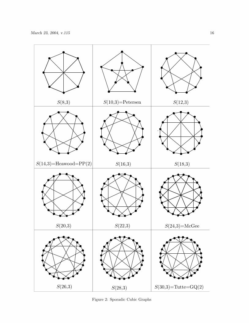
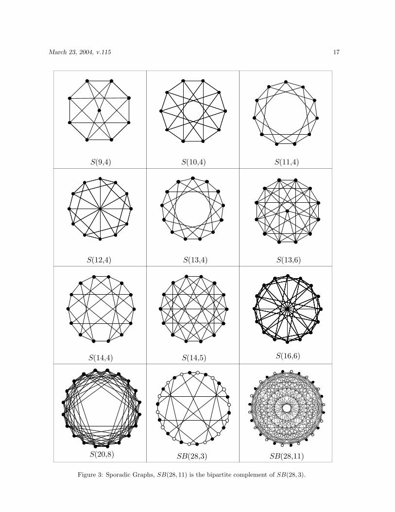
Other sporadic graphs are shown in Figure 3. We prove these are trace-minimal in Section 6.

March 23, 2004, v.115 16

S(8,3)

S(22,3) S(24,3)=McGee

S(10,3)=Petersen

S(14,3)=Heawood=PP(2)

S(30,3)=Tutte=GQ(2)

S(16,3) S(18,3)

S(12,3)

S(20,3)

S(26,3) S(28,3)

Figure 2: Sporadic Cubic Graphs

March 23, 2004, v.115 17

S(14,5)

S(9,4)

S(12,4) S(13,4) S(13,6)

S(16,6)

S(10,4) S(11,4)

S(14,4)

S(20,8) SB(28,3) SB(28,11)

Figure 3: Sporadic Graphs, SB(28, 11) is the bipartite complement of SB(28, 3).

March 23, 2004, v.115 18

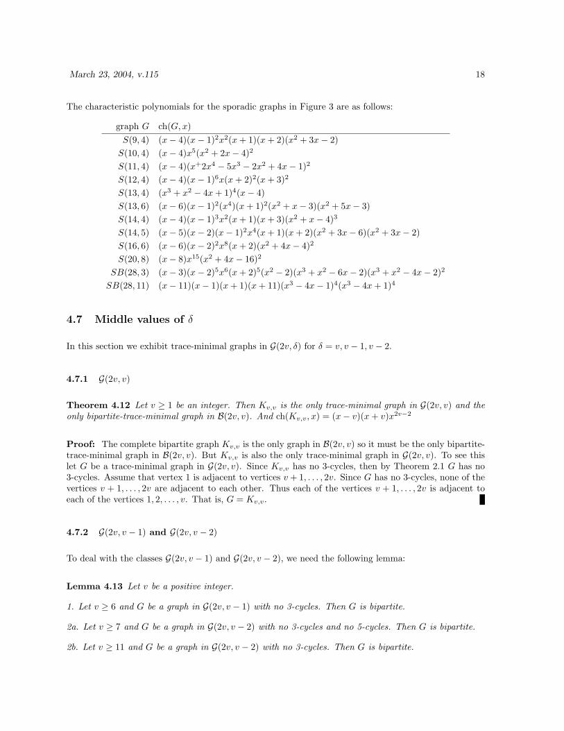
The characteristic polynomials for the sporadic graphs in Figure 3 are as follows:

graph G ch(G, x)S(9, 4) (x− 4)(x− 1)2x2(x + 1)(x + 2)(x2 + 3x− 2)

S(10, 4) (x− 4)x5(x2 + 2x− 4)2

S(11, 4) (x− 4)(x+2x4 − 5x3 − 2x2 + 4x− 1)2

S(12, 4) (x− 4)(x− 1)6x(x + 2)2(x + 3)2

S(13, 4) (x3 + x2 − 4x + 1)4(x− 4)S(13, 6) (x− 6)(x− 1)2(x4)(x + 1)2(x2 + x− 3)(x2 + 5x− 3)S(14, 4) (x− 4)(x− 1)3x2(x + 1)(x + 3)(x2 + x− 4)3

S(14, 5) (x− 5)(x− 2)(x− 1)2x4(x + 1)(x + 2)(x2 + 3x− 6)(x2 + 3x− 2)S(16, 6) (x− 6)(x− 2)2x8(x + 2)(x2 + 4x− 4)2

S(20, 8) (x− 8)x15(x2 + 4x− 16)2

SB(28, 3) (x− 3)(x− 2)5x6(x + 2)5(x2 − 2)(x3 + x2 − 6x− 2)(x3 + x2 − 4x− 2)2

SB(28, 11) (x− 11)(x− 1)(x + 1)(x + 11)(x3 − 4x− 1)4(x3 − 4x + 1)4

4.7 Middle values of δ

In this section we exhibit trace-minimal graphs in G(2v, δ) for δ = v, v − 1, v − 2.

4.7.1 G(2v, v)

Theorem 4.12 Let v ≥ 1 be an integer. Then Kv,v is the only trace-minimal graph in G(2v, v) and theonly bipartite-trace-minimal graph in B(2v, v). And ch(Kv,v, x) = (x− v)(x + v)x2v−2

Proof: The complete bipartite graph Kv,v is the only graph in B(2v, v) so it must be the only bipartite-trace-minimal graph in B(2v, v). But Kv,v is also the only trace-minimal graph in G(2v, v). To see thislet G be a trace-minimal graph in G(2v, v). Since Kv,v has no 3-cycles, then by Theorem 2.1 G has no3-cycles. Assume that vertex 1 is adjacent to vertices v + 1, . . . , 2v. Since G has no 3-cycles, none of thevertices v + 1, . . . , 2v are adjacent to each other. Thus each of the vertices v + 1, . . . , 2v is adjacent toeach of the vertices 1, 2, . . . , v. That is, G = Kv,v.

4.7.2 G(2v, v − 1) and G(2v, v − 2)

To deal with the classes G(2v, v − 1) and G(2v, v − 2), we need the following lemma:

Lemma 4.13 Let v be a positive integer.

1. Let v ≥ 6 and G be a graph in G(2v, v − 1) with no 3-cycles. Then G is bipartite.

2a. Let v ≥ 7 and G be a graph in G(2v, v − 2) with no 3-cycles and no 5-cycles. Then G is bipartite.

2b. Let v ≥ 11 and G be a graph in G(2v, v − 2) with no 3-cycles. Then G is bipartite.

March 23, 2004, v.115 19

Proof: Assume G is not bipartite and has no 3-cycles. Then G has an odd cycle of length at least5. Let 1, . . . ,m be the vertices of the shortest odd cycle in G. No two vertices i, j among 1, . . . ,m areadjacent unless i− j = ±1 (mod m) since any other edge would become part of a shorter odd cycle. Foreach i = 1, . . . ,m, let Ai be the set of vertices adjacent to vertex i excluding vertices i± 1 in the cycle.Clearly, Ai ∩Aj = ∅ unless i = j or i− j ≡ ±2 (mod m), since any such nonempty intersection would bepart of a shorter odd cycle.

1. Let G ∈ G(2v, v−1). In this case |Ai| = v−3 for all i. Since A1∩A2 = ∅, we have 2v ≥ m+ |A1∪A2| =m + 2(v − 3) and hence m ≤ 6. It follows that m = 5. Next we show that |A1 ∩ A3| ≥ v − 4. SinceA1 ∩A2 = A2 ∩A3 = ∅,

2v − 5 ≥ |A1 ∪A2 ∪A3| = |A1|+ |A2|+ |A3| − |A1 ∩A3| = 3(v − 3)− |A1 ∩A3|.

Similarly |A3 ∩A5| ≥ v − 4. Since A1 and A5 are disjoint,

v − 3 = |A3| ≥ |A1 ∩A3|+ |A3 ∩A5| = 2(v − 4).

Thus v ≤ 5.

2. Let G ∈ G(2v, v − 2). In this case |Ai| = v − 4 for all i. Arguing as above, we get 2v ≥ m + 2(v − 4)so that m ≤ 8. Thus m = 5 or m = 7.

Consider first the case m = 7. Since A1 ∩A2 = A2 ∩A3 = ∅,

2v − 7 ≥ |A1 ∪A2 ∪A3| = |A1|+ |A2|+ |A3| − |A1 ∩A3| = 3(v − 4)− |A1 ∩A3|.

Thus |A1 ∩A3| ≥ v − 5 and likewise |A3 ∩A5| ≥ v − 5. We have A1 ∩A5 = ∅. So

v − 4 = |A3| ≥ |A1 ∩A3|+ |A3 ∩A5| ≥ 2(v − 5).

It follows that v ≤ 6.

Now consider the case m = 5. In this case, |A1 ∩A3| ≥ v− 7. The reason is that A1 ∩A2 = A2 ∩A3 = ∅.Thus

2v − 5 ≥ |A1 ∪A2 ∪A3| = |A1|+ |A2|+ |A3| − |A1 ∩A3| = 3(v − 4)− |A1 ∩A3|.

Likewise, |A3 ∩A5| ≥ v − 7.

Now since A1 ∩A5 = ∅, we have

v − 4 = |A3| ≥ |A1 ∩A3|+ |A3 ∩A5| ≥ 2(v − 7).

So v ≤ 10.

Theorem 4.14 Let v ≥ 1 be an integer. The trace-minimal graph in G(2v, v − 1) is unique and is given(along with ch(G, x)) as follows:

v graph G ch(G, x)v 6= 4, 5 Kv,v − vK2 (x2 − (v − 1)2)(x2 − 1)v−1

v = 4 S(8, 3) (x− 3)(x− 1)2(x + 1)(x2 + 2x− 1)2

v = 5 S(10, 4) (x− 4)x5(x2 + 2x− 4)2

March 23, 2004, v.115 20

Proof: Let G be a trace-minimal graph in G(2v, v−1). The graph Kv,v−vK2 ∈ G(2v, v−1) is bipartiteand has no 3-cycles. Thus G has no 3-cycles by Theorem 2.1. If v ≥ 6, it follows from Lemma 4.13 thatG is bipartite. But the only bipartite graph in G(2v, v − 1) is Kv,v − vK2 so G = Kv,v − vK2.

If v = 1, 2 the only graph in G(2v, v − 1) is Kv,v − vK2 so again G = Kv,v − vK2. The only remainingcases are v = 3, 4, 5. But C6 = K3,3 − 3K2 was shown to be trace-minimal in G(6, 2) in Lemma 4.2. Thecases v = 4, 5 are proved in Lemmas 6.1 and 6.3.

It is easy to see that the adjacency matrix for Kv,v − vK2 is a 2× 2 block matrix in which the diagonalblocks are zero and the off-diagonal blocks are J − I. The computation for the characteristic polynomialis routine.

Theorem 4.15 Let v ≥ 2 be an integer. The trace-minimal graph G in G(2v, v − 2) is unique.

If v 6= 5, 6, 7, 8, 10, then G = Kv,v − C2v with characteristic polynomial

ch(G, x) =x2 − (v − 2)2

x2 − 4(2Tch2v(x/2)− 2) .

For v = 5, 6, 7, 8, 10, the trace-minimal graph G and its characteristic polynomial are given in the table:

v graph G ch(G, x)v = 5 Petersen (x− 3)(x− 1)5(x + 2)4

v = 6 S(12, 4) (x− 4)(x− 1)6x(x + 2)2(x + 3)2

v = 7 S(14, 5) (x− 5)(x− 2)(x− 1)2x4(x + 1)(x + 2)(x2 + 3x− 6)(x2 + 3x− 2)v = 8 S(16, 6) (x− 6)(x− 2)2x8(x + 2)(x2 + 4x− 4)2

v = 10 S(20, 8) (x− 8)x15(x2 + 4x− 16)2

Proof: Let G be a trace-minimal graph in G(2v, v − 2). The graph Kv,v − C2v ∈ G(2v, v − 2) isbipartite and has no 3-cycles. Thus G has no 3-cycles. If v ≥ 11, it follows from Lemma 4.13 that Gis bipartite. But from Lemma 4.2 the only bipartite-trace-minimal graph in G(2v, v − 2) is Kv,v − C2v.Thus G = Kv,v − C2v.

For v ≤ 5, I4 = K2,2 − C4, 3K2 = K3,3 − C6, C8 = K4,4 − C8, and the Petersen graph, were proved tobe trace-minimal in Lemmas 4.1, 4.2, and 4.3.

The cases v = 6, 7, 8, 10 are analyzed in Lemma 6.4. Finally, the proof that K9,9 − C18 is trace-minimalin G(18, 7) is given in Lemma 6.5.

4.8 Large values of δ

In this section we exhibit trace-minimal graphs in G(v, δ) for all v and v − 6 ≤ δ ≤ v − 1. (Note that forδ = v − 2, v − 4, v − 6, v must be even.)

March 23, 2004, v.115 21

4.8.1 δ = v − 1, v − 2

See Lemma 4.1.

4.8.2 δ = v − 3

Lemma 4.16 Let v ≥ 3 be an integer. The trace-minimal graph G in G(v, v − 3) is unique and is given(along with ch(G, x)) as follows:

v (mod 3) graph G ch(G, x)v = 3l I

(l)3 (x− (v − 3))x2l(x + 3)l−1

v = 3l + 1 2K2 5 I(l−1)3 (x− (v − 3))x2l−2(x + 3)l−1(x + 1)2(x− 1)

v = 3l + 2 C5 5 I(l−1)3 (x− (v − 3))x2l−2(x + 3)l−1(x2 + x− 1)2.

4.8.3 δ = v − 4

Lemma 4.17 Let v ≥ 4 be an even integer. The trace-minimal graph G in G(v, v − 4) is unique and isgiven (along with ch(G, x)) as follows:

v (mod 4) graph G ch(G, x)v = 4l I

(l)4 (x− (v − 4))x3l(x + 4)l−1

v = 4l + 2 C6 5 I(l−1)4 (x− (v − 4))(x− 1)2x3l−3(x + 1)2(x + 2)(x + 4)l−1.

4.8.4 δ = v − 5

Lemma 4.18 Let v ≥ 5 be an integer. The trace-minimal graph G in G(v, v − 5) is unique and is given(along with chG(x)) as follows:

v graph G ch(G, x)v = 5l I

(l)5 (x− (v − 5))x4l(x + 5)l−1

v = 5l + 1 3K2 5 I(l−1)5 (x− (v − 5))(x− 1)2x4l−4(x + 1)3(x + 5)l−1

v = 5l + 2 C7 5 I(l−1)5 (x− (v − 5))x4l−4(x + 5)l−1(x3 + x2 − 2x− 1)2

v = 5l + 3 S(8, 3)5 I(l−1)5 (x− (v − 5))(x− 1)2x4l−4(x + 1)(x + 5)l−1(x2 + 2x− 1)2

v = 5l + 4 S(9, 4)5 I(l−1)5 (x− (v − 5))(x− 1)2x4l−2(x + 1)(x + 2)(x + 5)l−1(x2 + 3x− 2)

4.8.5 δ = v − 6

Lemma 4.19 Let v ≥ 6 be an even integer. The trace-minimal graph G in G(v, v − 6) is unique and isgiven (along with ch(G, x)) as follows:

March 23, 2004, v.115 22

v graph G chG(x)v = 6l I

(l)6 (x− (v − 6))x5l(x + 6)l−1

v = 6l + 2 C8 5 I(l−1)6 (x− (v − 6)x5l−3(x + 2)(x + 6)l−1(x2 − 2)2

v = 6l + 4 S(10, 4)5 I(l−1)6 (x− (v − 6))x5l(x + 6)l−1(x2 + 2x− 4)2

4.9 Proofs for large δ

Many of the trace-minimal graphs in Section 4.8 are the unique graph in G(v, δ) with the fewest numberof triangles and hence trace-minimal by Theorem 2.1. Letting 4(G) denote the number of triangles(3-cycles) in G, it is easy to see that

4(G) =16trA(G)3.

It is useful to notice that if G ∈ G(v, δ) and Gcomp ∈ G(v, δ′) is the complement of G (δ + δ′ = v − 1),then

trA(G)3 + trA(Gcomp)3 = 6(

v

3

)− 3vδδ′.

Thus G has the fewest number of triangles in G(v, δ) if and only if Gcomp has the largest number oftriangles in G(v, δ′). In the following sections, it is convenient to deal with graphs having the largestnumber of triangles instead of the smallest number of triangles. We denote the minimum and maximumnumber of triangles in a graph class as follows:

min4(v, δ) = minimum{4(G) : G ∈ G(v, δ)}max4(v, δ) = maximum{4(G) : G ∈ G(v, δ)}

By the comments above, we have

min4(v, δ) + max4(v, δ′) =(

v

3

)− 1

2vδδ′, (14)

where δ + δ′ = v − 1.

In the next few results, we shall see that for δ′ ≤ 5, all but one component of the graph in G(v, δ′) withthe largest number of triangles are the complete graph Kδ′+1. And that the other component H hasfewer than 2δ′ + 2 vertices. Thus, by the remarks above, the graph in G(v, δ) with the fewest number oftriangles is of the form (H + kKδ′+1)comp = Hcomp 5 I

(k)δ′+1, for some nonnegative integer k.

Let i be a vertex of a graph G and define 4(G, i) to be the number of triangles in G in which i is avertex. Likewise if (i, j) is an edge in G, let 4(G, (i, j)) denote the number of triangles in G that includeedge (i, j).

Theorem 4.20 Let δ ≥ 3 and G ∈ G(v, δ). If 4(G) = max4(v, δ) then either Kδ+1 is a component ofG or 4(G, x) ≤

(δ2

)− 2 for all vertices x in G.

Proof: Assume G ∈ G(v, δ), 4(G) = max4(v, δ), and 4(G, u) >(δ2

)− 2 for some vertex u in G. Let

N be the subgraph of δ + 1 vertices consisting of u and all vertices adjacent to u. If 4(G, u) =(δ2

),

March 23, 2004, v.115 23

then N = Kδ+1 is a component of G. Thus we shall assume that 4(G, u) =(δ2

)− 1. Then every pair of

vertices in N are adjacent except one pair, say vertex 1 and vertex 2. Thus no vertex in N is adjacent toa vertex not in N , except for vertex 1 and vertex 2. However, each of these two vertices must be adjacentto exactly one vertex that is not in N . If vertices 1 and 2 are adjacent to the same vertex not in N , welabel it vertex 3. If they are adjacent to different vertices not in N , we shall label these vertices 3 and 4and assume that (1,3) and (2,4) are edges in G.

In either case, we construct a graph H ∈ G(v, δ) by removing at least the two edges, (1,3) and (2,3), or (1,3)and (2,4), from G and adding edge (1,2) and others to obtain H. Since 4(G, (1, 3)) = 4(G, (2, 4)) = 0,no triangles are lost from G by removing these two edges. However, when we add edge (1,2) to get H,Kδ+1 is a component of H and we gain 4(H, (1, 2)) = δ − 1 triangles. In each of the four cases below,the number of triangles in H exceeds the number of triangles in G, contradicting the assumption that4(G) = max4(v, δ).

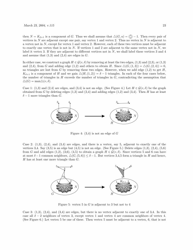
Case 1: (1,3) and (2,4) are edges, and (3,4) is not an edge. (See Figure 4.) Let H ∈ G(v, δ) be the graphobtained from G by deleting edges (1,3) and (2,4) and adding edges (1,2) and (3,4). Then H has at leastδ − 1 more triangles than G.

N

G

1 2

3 4

N

H

1 2

3 4

Kd+1

Figure 4: (3,4) is not an edge of G

Case 2: (1,3), (2,4), and (3,4) are edges, and there is a vertex, say 5, adjacent to exactly one of thevertices 3,4. Say (3,5) is an edge but (4,5) is not an edge. (See Figure 5.) Delete edges (1,3), (2,4), (5,6)from G and add edges (1,2), (3,6), (4,5) to obtain a graph H ∈ G(v, δ). Since vertices 5 and 6 can haveat most δ− 1 common neighbors, 4(G, (5, 6)) ≤ δ− 1. But vertices 3,4,5 form a triangle in H and hence,H has at least one more triangle than G.

N

G

1 2

35 6

4

N

H

1 2Kd+1

35 6

4

Figure 5: vertex 5 in G is adjacent to 3 but not to 4

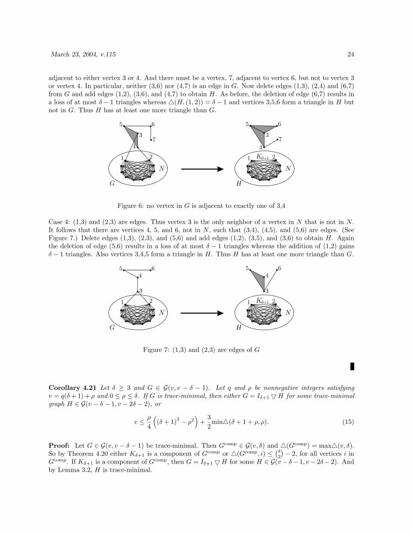
Case 3: (1,3), (2,4), and (3,4) are edges, but there is no vertex adjacent to exactly one of 3,4. In thiscase all δ − 2 neighbors of vertex 3, except vertex 1 and vertex 4 are common neighbors of vertex 4.(See Figure 6.) Let vertex 5 be one of these. Then vertex 5 must be adjacent to a vertex, 6, that is not

March 23, 2004, v.115 24

adjacent to either vertex 3 or 4. And there must be a vertex, 7, adjacent to vertex 6, but not to vertex 3or vertex 4. In particular, neither (3,6) nor (4,7) is an edge in G. Now delete edges (1,3), (2,4) and (6,7)from G and add edges (1,2), (3,6), and (4,7) to obtain H. As before, the deletion of edge (6,7) results ina loss of at most δ − 1 triangles whereas 4(H, (1, 2)) = δ − 1 and vertices 3,5,6 form a triangle in H butnot in G. Thus H has at least one more triangle than G.

N

G

1 2

3

5 6

7 7

4

N

H

1 2Kd+1

3

5 6

4

Figure 6: no vertex in G is adjacent to exactly one of 3,4

Case 4: (1,3) and (2,3) are edges. Thus vertex 3 is the only neighbor of a vertex in N that is not in N .It follows that there are vertices 4, 5, and 6, not in N , such that (3,4), (4,5), and (5,6) are edges. (SeeFigure 7.) Delete edges (1,3), (2,3), and (5,6) and add edges (1,2), (3,5), and (3,6) to obtain H. Againthe deletion of edge (5,6) results in a loss of at most δ − 1 triangles whereas the addition of (1,2) gainsδ − 1 triangles. Also vertices 3,4,5 form a triangle in H. Thus H has at least one more triangle than G.

N

G

1 2

3

5 6

4

N

H

1 2Kd+1

3

5 6

4

Figure 7: (1,3) and (2,3) are edges of G

Corollary 4.21 Let δ ≥ 3 and G ∈ G(v, v − δ − 1). Let q and ρ be nonnegative integers satisfyingv = q(δ + 1) + ρ and 0 ≤ ρ ≤ δ. If G is trace-minimal, then either G = Iδ+15H for some trace-minimalgraph H ∈ G(v − δ − 1, v − 2δ − 2), or

v ≤ ρ

4

((δ + 1)2 − ρ2

)+

32min4(δ + 1 + ρ, ρ). (15)

Proof: Let G ∈ G(v, v − δ − 1) be trace-minimal. Then Gcomp ∈ G(v, δ) and 4(Gcomp) = max4(v, δ).So by Theorem 4.20 either Kδ+1 is a component of Gcomp or 4(Gcomp, i) ≤

(δ2

)− 2, for all vertices i in

Gcomp. If Kδ+1 is a component of Gcomp, then G = Iδ+15H for some H ∈ G(v− δ− 1, v− 2δ− 2). Andby Lemma 3.2, H is trace-minimal.

March 23, 2004, v.115 25

Otherwise, 4(Gcomp, i) ≤(δ2

)− 2 for all vertices, i of G. Thus

max4(v, δ) = 4(Gcomp) =13

∑4(Gcomp, i) ≤ v

3

[(δ

2

)− 2]

, (16)

where the sum is taken over all vertices, i of Gcomp. Let G1 = (q − 1)Kδ+1 + H ∈ G(v, δ), whereH ∈ G(δ + 1 + ρ, δ) satisfies 4(H) = max4(δ + 1 + ρ, δ). Then

max4(v, δ) ≥ 4(G1) = (q − 1)(

δ + 13

)+ max4(δ + 1 + ρ, δ). (17)

By Equation (14),

max4(δ + 1 + ρ, δ) =(

δ + 1 + ρ

3

)− 1

2δρ(δ + 1 + ρ)−min4(δ + 1 + ρ, ρ). (18)

Thus, by (16), (17), and (18), we have

v

3

[(δ

2

)− 2]≥ (q − 1)

(δ + 1

3

)+(

δ + 1 + ρ

3

)− 1

2δρ(δ + 1 + ρ)−min4(δ + 1 + ρ, ρ),

which implies (15).

We also need a result by Pullman and Wormald [PW]:

Lemma 4.22 [PW] There exists a graph G ∈ G(v, δ) with 4(G) = 0 if and only if 2δ < v for v even or5δ < 2v for v odd.

4.9.1 Proof of Lemma 4.16

Let v ≥ 3 be an integer and let G be a trace-minimal graph in G(v, v− 3). Then 4(G) = min4(v, v− 3),Gcomp ∈ G(v, 2), and 4(Gcomp) = max4(v, 2). Every graph in G(v, 2) is a direct sum of its cycliccomponents. Thus all or all but one of the components of Gcomp must be 3-cycles. If v = 3l, thenGcomp = lC3 and G = I

(l)3 . If v = 3l + 1, then Gcomp = C4 + (l − 1)C3 and G = (C4)comp 5 I

(l−1)3 =

2K25 I(l−1)3 . And if v = 3l + 2, then Gcomp = C5 + (l− 1)C3 and G = C55 I

(l−1)3 , since (C5)comp = C5.

To compute the characteristic polynomials ch(G, x) we need ch(C3, x) = (x − 2)(x + 1)2, ch(C4, x) =x2(x + 2)(x− 2) and ch(C5, x) = (x− 2)(x2 + x− 1)2.

Suppose v = 3l + 1. Then Gcomp = C4 + (l − 1)C3. Thus ch(Gcomp, x) = ch(C4, x)[ch(C3, x)]l−1 and byEquation (10)

ch(G, x) = ±(x− (v − 3))(−x− 1)2((−x− 1) + 2)((−x− 1)− 2)[(−x− 1)− 2)((−x− 1) + 1)2]l−1/(x + 3)= (x− (v − 3))(x + 1)2(x− 1)(x + 3)l−1x2l−2.

The characteristic polynomials for other cases, v = 3l and 3l + 2 are computed in a similar way.


Let v ≥ 4 be an even integer and let G be a trace-minimal graph in G(v, v − 4). Let v = 4l + ρ, whereρ = 0, 2. We apply Corollary 4.21 with δ = 3. If ρ = 0, then the right side of Inequality (15) is 0. Thus

March 23, 2004, v.115 26

by repeated application of Corollary 4.21, G = I(l−1)4 5H, where H is a trace-minimal graph in G(4, 0).

But then H = I4 and so G = I(l)4 .

Now suppose ρ = 2. Since min4(6, 2) = 0 (by Lemma 4.22), the right side of Inequality (15) is 6. ByCorollary 4.21, G = I

(l−1)4 5 H, where H is a trace-minimal graph in G(6, 2). Then by Lemma 4.2

H = C6.

To compute the characteristic polynomial of C65I(l−1)4 , we need ch(C6, x) = (x−2)(x−1)2(x+1)2(x+2)

from Lemma 4.2. It is easy to show that ch(I(l−1)4 , x) = (x−4(l−2))x3(l−1)(x+4)l−2. Thus from Equation

(11) we have

ch(G, x) = ± (x− (4l − 2))(x + 4)(x− 2)(x− 4(l − 2))

ch(C6, x)ch(I(l−1)4 , x)

= (x− (v − 4))(x + 4)l−1x3(l−1)(x− 1)2(x + 1)2(x + 2).

If v = 4l thench(G, x) = (x− (v − 4))x3l(x + 4)l−1.


Let v ≥ 5 be an integer and let G be a trace-minimal graph in G(v, v − 5) and let v = 5l + ρ, whereρ = 0, 1, 2, 3, 4. We apply Corollary 4.21 with δ = 4. Thus there are five cases.

First suppose ρ = 0. Then the right side of Inequality (15) is 0. By repeated application of Corollary4.21, G = I

(l−1)5 5H, where H is a trace-minimal graph in G(5, 0). Thus H = I5 and so G = I

(l)5 .

Now suppose ρ = 1. Then the right side of Inequality (15) is 6, since the matching 3K2 in G(6, 1) has notriangles. Thus G = I

(l−1)5 5H, where H is a trace-minimal graph in G(6, 1). Thus H = 3K2 by Lemma

4.1 and G = I(l−1)5 5 3K2.

For ρ = 2 the right side of Inequality (15) is 10.5. (The graph C7 has no triangles.) So G = I(l−1)5 5H,

where H is trace-minimal in G(7, 2). Then by Lemma 4.2, H = C7.

For ρ = 3 the right side of Inequality (15) is 12. (The graph S(8, 3) has no triangles; see Figure 2.) SoG = I

(l−1)5 5H, where H is trace-minimal in G(8, 3). Then by Lemma 6.1, H = S(8, 3).

For ρ = 4 the right side of Inequality (15) is 12, since S(9, 4) has two triangles, which is the minimum,min4(9, 4). (See Figure 3.) So G = I

(l−1)5 5H, where H is trace-minimal in G(9, 4). Then by Lemma

6.2, H = S(9, 4).

The characteristic polynomial of these graphs can be computed using Equation (11). It is not difficultto see that ch(I(l−1)

5 , x) = (x − 5(l − 2))x4l−4(x + 5)l−2. From Section 4.6 we have ch(S(8, 3), x) =(x − 3)(x − 1)2(x + 1)(x2 + 2x − 1)2. Now to compute the characteristic polynomial of S(8, 3)5 I

(l−1)5

we use Equation (11) with G1 = S(8, 3), G2 = I(l−1)5 . Then v1 = 8, δ1 = 3, v2 = 5(l − 1), δ2 = 5(l − 2)

March 23, 2004, v.115 27

and so v = 5l + 3, δ = 5l − 2. Thus,

ch(S(8, 3)5 I(l−1)5 , x) =

(ch(S(8, 3), x)

x− 3

)(ch(I(l−1)

5 , x)x− 5(l − 2)

)(x− (5l − 2))(x + 5)

= (x− 1)2(x + 1)(x2 + 2x− 1)2x4l−4(x + 5)l−2(x− (5l − 2))(x + 5)= (x− (5l − 2))(x− 1)2x4l−4(x + 1)(x + 5)l−1(x2 + 2x− 1)2.

The characteristic polynomials for the remaining cases are computed in a similar way.


Let v ≥ 6 be an even integer. Let G be a trace-minimal graph in G(v, v − 6) and let v = 6l + ρ whereρ = 0, 2, 4. We apply Corollary 4.21 with δ = 5.

If ρ = 0 then the right side of Equation (15) is 0. So by Corollary 4.21, G = I(l−1)6 5 H, where H is

trace-minimal in G(6, 0). Then H = I6 and G = I l6.

In the case ρ = 2, the right side of Equation (15) is 16. (The graph C8 has no triangles.) So Corollary4.21 implies that G = I

(l−2)6 5H with H trace-minimal in G(14, 8). Then H = I6 5 C8 by Lemma 6.6

and G = I(l−1)6 5 C8.

In the case ρ = 4, the right side of Equation (15) is 20, since S(10, 4) has no triangles. (See Figure 3.) Sothe Corollary 4.21 implies that G = I

(l−2)6 5H with H trace-minimal in G(16, 10). Then H = I65S(10, 4)

by Lemma 6.6 and G = I(l−1) 5 S(10, 4).

To compute the characteristic polynomials of these graphs, first note that ch(I(l)6 , x) = (x−6(l−1))x5l(x+

6)l−1, which follows from Equation (11) and ch(I6, x) = x6. Now using Equation (11) and the character-istic polynomial of S(10, 4) from Section 4.6, we have

ch(S(10, 4)5 I(l−1)6 , x)

(x + 6)(x− (6l − 2))=

(x− 4)x5(x2 + 2x− 4)2

x− 4· (x− 6(l − 2))x5l−5(x + 6)l−2

x− 6(l − 2),

and thusch(S(10, 4)5 I

(l−1)6 , x) = (x− (6l − 2))x5l(x + 6)l−1(x2 + 2x− 4)2.

The characteristic polynomial of C8 5 I(l−1)6 can be computed in a similar way.

5 Formulas for P (n, r, t)

In this section, we exhibit formulas for P (n, r, t) for various pairs (n, r) where n ≡ −1 (mod 4) and0 ≤ r < n. In each case, the formula is obtained from a corresponding (bipartite-)trace-minimal graphand its characteristic polynomial using one of the theorems from Section 1.3. Rather than writing theroutine calculation for each pair (n, r), we simply list the graph class and (bipartite-)trace-minimal graphin the class along with the section in which the graph and its characteristic polynomial are found andthe theorem and equation from Section 1.3 that is used. To illustrate the method, we will work out thecalculation in a few cases.

March 23, 2004, v.115 28

5.1 Strongly Regular

We begin with the formulas for P (n, r, t) that follow from the the strongly regular graphs with an evennumber of vertices and no 3-cycles. These are trace-minimal.

Theorem 5.1

P (19, 13, t) = 20(5t + 2)10(5t + 5)9

P (31, 21, t) = 32(8t + 4)20(8t + 8)11

P (99, 29, t) = 100(25t + 5)56(25t + 10)42(25t + 25)P (111, 41, t) = 112(28t + 8)70(28t + 14)40(28t + 28)P (199, 89, t) = 200(50t + 20)154(50t + 30)44(50t + 50).

The following table gives the graph class and a trace-minimal graph in the class corresponding to eachpair (n, r). Since r ≡ 1 (mod 4) in all cases, we use Theorem 1.2 and Equation (3) from Section 1.3. Thecharacteristic polynomials for each graph is given in Section 4.3.

(n, r) class graph G or B

(19, 13) G(10, 3) Petersen(31, 21) G(16, 5) Clebsh(99, 29) G(50, 7) Hoffman-Singleton

(111, 41) G(56, 10) Gewirtz(199, 89) G(100, 22) Higman-Sims

As an example, take (n, r) = (99, 29). Then p = 25 and d = 7. From Theorem 1.2, we seek a trace-minimal graph in G(2p, d), where (2p, d) = (50, 7) The Hoffman-Singleton graph G is trace-minimal inG(50, 7) and has characteristic polynomial ch(G, x) = (x− 7)(x− 2)28(x + 3)21. (See Section 4.3.) FromTheorem 1.2, Equation (3) we have

P (99, 29, t) =4(t + 1)[ch(G, pt + d)]2

t2

=4(t + 1)[(25t)(25t + 5)28(25t + 10)21]2

t2,

which is equal to the expression for P (99, 29, t) given in Theorem 5.1.

5.2 Generalized polygons

In this section we give the formulas for P (n, r, t) that correspond to the incidence graphs of generalizedpolygons, all of which are trace-minimal.

March 23, 2004, v.115 29

5.2.1 Finite projective planes

Theorem 5.2 Let Γ be a finite projective plane of order q on p = q2 + q + 1 points and lines, and letn = 4p− 1. Then

P (n, 4q + 5, t) = 4p(pt + p)(pt + 2q + 2)2((pt + q + 1)2 − q)2p−2.

In particular, for the finite projective plane of order q = 2 on seven points,

P (27, 13, t) = 28(7t + 7)(7t + 6)2(49t2 + 42t + 7)12,

which is one of the formulas in Theorem 5.23.

Let d = q + 1. The incidence graph PP (q) of Γ is a trace-minimal d-regular graph in G(2p, q + 1) withch(PP (q), x) = (x2 − (q + 1)2)(x2 − q)p−1. (See Section 4.4.1.) Since r = 4q + 5 ≡ 1 (mod 4), Theorem5.2 follows from Theorem 1.2 as follows:

P (n, 4q + 5, t) =4(t + 1)[ch(PP (q), pt + q + 1)]2

t2

=4(t + 1)(pt)2(pt + 2q + 2)2[(pt + q + 1)2 − q]2p−2

t2

= 4p(pt + p)(pt + 2q + 2)2((pt + q + 1)2 − q)2p−2.

5.2.2 Generalized quadrangles

Let q be a power of a prime, let Γ be the generalized quadrangle and GQ(q) the incidence graph of Γdescribed in Section 4.4.2. Then GQ(q) is a (q + 1)-regular bipartite graph on v = 2(q4 − 1)/(q − 1)vertices that is trace-minimal in G(v, q + 1) and hence bipartite-trace-minimal in B(v, q + 1). And fromLemma 4.7, the characteristic polynomial of A(GQ(q)) is

ch(GQ(q), x) = x2a(x2 − 2q)b(x2 − (q + 1)2),

where a = q(q2 + 1)/2, and b = q(q + 1)2/2. Then

(pt + d)2 − 2q = (pt)2 + 2(q + 1)pt + q2 + 1,

(pt + d)2 − (q + 1)2 = pt(pt + 2(q + 1)),

and soch(GQ(q), pt + d) = (pt + q + 1)2a((pt)2 + 2(q + 1)pt + q2 + 1)bpt(pt + 2(q + 1)).

Since the generalized quadrilateral graph GQ(q) is trace-minimal and bipartite-trace-minimal (Section4.4.2), it can be used in conjunction with Theorems 1.2, 1.4, and 1.5 to obtain three formulas for P (n, r, t).

The first formula comes from the fact that GQ(q) is in G(2p, q+1), where p = q3+q2+q+1 = (q+1)(q2+1).We use Theorem 1.2 with r = 4d + 1 = 4q + 5. Thus

4(t + 1)[ch(GQ(q), pt + d)]2

t2

= 4p(pt + p)(pt + q + 1)2q(q2+1)

×((pt)2 + 2(q + 1)pt + q2 + 1)q(q+1)2(pt + 2(q + 1))2,

which proves the next theorem.

March 23, 2004, v.115 30

Theorem 5.3 Let q be a power of a prime, and p = (q + 1)(q2 + 1) and let n = 4p− 1. Then

P (n, 4q + 5, t)

= 4p(pt + p))(pt + q + 1)2q(q2+1)((pt)2 + 2(q + 1)pt + q2 + 1)q(q+1)2(pt + 2(q + 1))2.

Our next formula comes from the fact that GQ(q) ∈ B(4p, q +1), where p = (q +1)(q2 +1)/2. (Since q isodd, p is an integer.) Let r = 4d− 1 = 4q + 3. Then d < p/2, p(t− 1) + 2d = pt− (q + 1)(q2 + 1)/2, and

4(p(t− 1) + 2d)ch(GQ(q), pt + d)t(pt + 2d)

= 4p(pt− (q + 1)(q2 − 3)/2)(pt + q + 1)q(q2+1)

×((pt)2 + 2(q + 1)pt + q2 + 1)q(q+1)2/2.

Using Theorem 1.4, we have proved the next theorem.

Theorem 5.4 Let q be a power of an odd prime, p = (q + 1)(q2 + 1)/2, and n = 4p− 1. Then

P (n, 4q + 3, t)

= 4p(pt− (q + 1)(q2 − 3)/2)(pt + q + 1)q(q2+1)((pt)2 + 2(q + 1)pt + q2 + 1)q(q+1)2/2.

Finally, Theorem 1.5 applies to the incidence graph GQ(q) ∈ G(4p, q + 1), where r = 4d, and p =(q + 1)(q2 + 1)/2. Then d ≤ p/2 and

4ch(GQ(q), (pt + d))t

= 4p(pt + q + 1)q(q2+1)(pt + 2(q + 1))[(pt)2 + 2(q + 1)pt + q2 + 1]q(q+1)2/2.

Thus we have the next theorem.

Theorem 5.5 Let q be a power of an odd prime, p = (q + 1)(q2 + 1)/2, and n = 4p− 1. Then

P (n, 4q + 4, t) = 4p(pt + q + 1)q(q2+1)(pt + 2(q + 1))[(pt)2 + 2(q + 1)pt + q2 + 1]q(q+1)2/2.

5.2.3 Generalized hexagons

Let q be a power of a prime, let Γ be the generalized hexagon and GH(q) the incidence graph of Γdescribed in Section 4.4.3. Then GH(q) is a (q+1)-regular bipartite graph on v = 2(q6−1)/(q−1) verticesthat is trace-minimal in G(v, q + 1) and hence bipartite-trace-minimal in B(v, q + 1). The characteristicpolynomial of A(GH(q)) is

ch(GH(q), x) = x2a(x2 − q

)b (x2 − 3q

)c(x2 − (q + 1)2)

where a = q(q2 + q + 1)(q2 − q + 1)/3, b = q(q2 − q + 1) (q + 1)2 /2 , and c = q (q + 1)2 (q2 + q + 1)/6.Throughout this section d = q + 1. Thus

(pt + d)2 − q = (pt)2 + 2 (q + 1) pt + q2 + q + 1,

(pt + d)2 − 3q = (pt)2 + 2 (q + 1) pt + q2 − q + 1,

(pt + d)2 − (q + 1)2 = pt (pt + 2(q + 1)) ,

March 23, 2004, v.115 31

and so

ch(GH(q), pt + d) = (pt + q + 1)2a((pt)2 + 2 (q + 1) pt + q2 + q + 1

)b

((pt)2 + 2 (q + 1) pt + q2 − q + 1

)c

pt (pt + 2(q + 1)) .

Since GH(q) is trace-minimal and bipartite-trace-minimal, it can be used in conjunction with Theorems1.2, 1.4, and 1.5 to obtain three formulas for P (n, r, t) .

First, GH(q) is in G(2p, q +1) where p = (q6− 1)/(q− 1). We use Theorem 1.2 with r = 4d +1 = 4q +5.We have

4(t + 1) [ch(GH(q), pt + d)]2

t2= 4p2(t + 1) (pt + 2(q + 1))2 (pt + q + 1)4a

×((pt)2 + 2 (q + 1) pt + q2 + q + 1

)2b ((pt)2 + 2 (q + 1) pt + q2 − q + 1

)2c

.


Theorem 5.6 Let q be a power of a prime, and p = (q6 − 1)/(q − 1) and let n = 4p− 1. Then

P (n, 4q + 5, t) = 4p2(t + 1) (pt + 2(q + 1))2 (pt + q + 1)4a

×((pt)2 + 2 (q + 1) pt + q2 + q + 1

)2b ((pt)2 + 2 (q + 1) pt + q2 − q + 1

)2c

.

Next, let r = 4q + 3 = 4d − 1. In this case we use Theorem 1.4 with GH(q) ∈ B(4p, q + 1), wherep = (q6−1)/2(q−1). (Since q is odd, p is an integer.) Then d < p/2, p(t−1)+2d = pt−(q+1)(q4+q2−3)/2,and

4(p(t− 1) + 2d)ch(G, pt + d)t(pt + 2d)

= 4p(pt− (q + 1)(q4 + q2 − 3)/2)(pt + q + 1)2a

×((pt)2 + 2 (q + 1) pt + q2 + q + 1

)b ((pt)2 + 2 (q + 1) pt + q2 − q + 1

)c

.


Theorem 5.7 Let q be a power of an odd prime, and p = (q6 − 1)/2(q − 1) and let n = 4p− 1. Then

P (n, 4q + 3, t) = 4p(pt− (q + 1)(q4 + q2 − 3)/2)(pt + q + 1)2a

×((pt)2 + 2 (q + 1) pt + q2 + q + 1

)b ((pt)2 + 2 (q + 1) pt + q2 − q + 1

)c

.

Finally, let r = 4d = 4q + 4. In this case we use Theorem 1.5 with GH(q) ∈ G(4p, q + 1), wherep = (q6 − 1)/2(q − 1). Then d ≤ p/2 and

4ch(G, pt + d)t

= 4p(pt + 2(q + 1)) (pt + q + 1)2a

×((pt)2 + 2 (q + 1) pt + q2 + q + 1

)b ((pt)2 + 2 (q + 1) pt + q2 − q + 1

)c

.


March 23, 2004, v.115 32

Theorem 5.8 Let q be a power of an odd prime, and p = (q6 − 1)/2(q − 1) and let n = 4p− 1. Then

P (n, 4q + 4, t) = 4p(pt + 2(q + 1)) (pt + q + 1)2a

×((pt)2 + 2 (q + 1) pt + q2 + q + 1

)b ((pt)2 + 2 (q + 1) pt + q2 − q + 1

)c

.

5.3 Large r

In this section we give formulas for P (n, r, t) for all pairs (n, r) satisfying n − 21 ≤ r ≤ n − 1 exceptr = n− 10, n− 11, n− 14, n− 15. These exceptional values of r require (bipartite-) trace-minimal graphsin G(2p, p− 3), B(4p, 2p− 3), G(2p, p− 4), and B(4p, 2p− 4). We have not analyzed these cases.

We assume throughout that p is a positive integer and n = 4p−1. Some of the formulas in this section donot hold for some small values of n. For example, the formula in the first part of Theorem 5.10 does nothold for n = 15, 19. We will not, however, restate the formulas for P (n, r, t) for n = 3, 7, 11, 15, 19, 23, 27as they appear either in [AFNW] or in Section 5.5, 5.6, or 5.7.

5.3.1 r = n− 1, n− 3, n− 4, n− 5

Theorem 5.9

P (n, n− 1, t) = 4p(pt)(pt + p)4p−2

P (n, n− 3, t) = 4p(pt + 2p− 2)(pt + p− 2)2p−1(pt + p)2p−1, for n ≥ 11P (n, n− 4, t) = 4p(pt + p)2p−1(pt + p− 2)2p, for n ≥ 7P (n, n− 5, t) = 4p(pt)(pt + p)2p−2(pt + p− 2)2p, for n ≥ 7.

The graphs that are required to prove the cases r = n−1, n−3, n−4, and n−5 of Theorem 5.9 appear inSection 4.1 and are given in the following table along with the appropriate theorem and equation, whichdepend on r (mod 4):

r class graph G Theorem/Equationn− 1 G(2p, 2p− 1) K2p 1.3 (4)n− 3 B(4p, 2p− 1) K2p,2p − 2pK2 1.5 (8)n− 4 G(4p, 4p− 2) I

(2p)2 1.4 (6)

n− 5 G(2p, 2p− 2) I(p)2 1.3 (4)

5.3.2 r = n− 2

Theorem 5.10 If n 6= 15, 19, then

P (n, n− 2, t) = 4p(pt + p)2p−1(pt + 2p− 2)2(pt + p− 2)2p−2.

Let r = n− 2 = 4p− 3 ≡ 1 (mod 4). Then Theorem 1.2 applies with d = p− 1. We seek a trace-minimalgraph in G(2p, p − 1). If p 6= 4, 5, then Kp,p − pK2 is trace minimal. See Section 4.7.2. For p = 4, 5 the

March 23, 2004, v.115 33

sporadic graph S(8, 3) is trace-minimal in G(8, 3) and S(10, 4) is trace-minimal in G(10, 4). See Section4.6. Theorem 5.10 now follows from Theorem 1.2.

5.3.3 r = n− 6

Theorem 5.11 If n ≥ 43 or n = 35, then

P (n, n− 6, t) = 4p(pt + 2p− 1)2

(pt + p)(pt + p− 4)2

[2Tch2p

(pt + p− 2

2

)− 2]2

. (19)

For n = 31, 39 we have

P (31, 25, t) = 32(8t + 4)4(8t + 6)16(8t + 8)3((8t)2 + 16(8t) + 56)4

P (39, 33, t) = 40(10t + 8)30(10t + 10)((10t)2 + 20(10t) + 80)4.

For r = n− 6 = 4p− 7 ≡ 1 (mod 4). Theorem 1.2 applies with d = p− 2. If p ≥ 11 or p = 9 (n ≥ 43 orn = 35), then G = Kp,p − C2p is a trace-minimal graph in G(2p, p− 2). (See Section 4.7.2.)

For p = 8, 10, the sporadic graph S(16, 6) is trace-minimal in G(16, 6) and S(20, 8) is trace-minimal inG(20, 8). (See Section 4.6.)

5.3.4 r = n− 7

Theorem 5.12 If n ≥ 19, then

P (n, n− 7, t) = 4ppt + 2p− 4

(pt + p)(pt + p− 4)

[2Tch4p

(pt + p− 2

2

)− 2]

.

For r = n − 7 = 4p − 8 ≡ 0 (mod 4), thus we use Theorem 1.5 with d = p − 2. Suppose p ≥ 5, that isn ≥ 19. Then p/2 < d and so Equation (8) of Theorem 1.5 applies. We seek a bipartite-trace-minimalgraph B in B(4p, 2p− 2). From Section 4.2, B = K2p,2p − C4p.

5.3.5 r = n− 8, n− 9

These formulas depend on the congruence class of n (mod 12). Let k be a positive integer.

Theorem 5.13 The polynomials P (n, n− 8, t) and P (n, n− 9, t) are given in the following tables:

n p P (n, n− 8, t)12k − 1 ≥ 23 3k 4p(pt + p− 3)8k(pt + p)4k−1

12k + 3 ≥ 15 3k + 1 4p(pt + p− 3)8k(pt + p)4k(pt + p− 2)2(pt + p− 4)12k + 7 ≥ 19 3k + 2 4p(pt + p− 3)8k+2(pt + p)4k+1((pt)2 + (2p− 5)(pt) + p2 − 5p + 5)2.

March 23, 2004, v.115 34

n p P (n, n− 9, t)12k − 1 ≥ 11 3k 4p(pt)(pt + p− 3)8k(pt + p)4k−2

12k + 3 ≥ 15 3k + 1 4p(pt)(pt + p− 3)8k−4(pt + p)4k−2((pt)2 + (2p− 5)(pt) + p2 − 5p + 5)4

12k + 7 ≥ 19 3k + 2 4p(pt)(pt + p− 3)8k(pt + p)4k(pt + p− 2)4(pt + p− 4)2.

Let r = n − 8 = 4p − 9 ≡ −1 (mod 4). Thus we use Theorem 1.4 with d = p − 2. Since p/2 ≤ dfor p ≥ 4, Equation (5) of Theorem 1.4 applies. We seek a trace-minimal graph in G(4p, 4p − 3). Thedescription depends on the congruence class of v (mod 3). Since v = 4p we must consider the casesv ≡ 0, 4, 8 (mod 12). Lemma 4.16 describes the trace-minimal graphs in G(v, v − 3), which we describein the following table:

n p graph class graph12k − 1 ≥ 23 3k G(12k, 12k − 3) I

(4k)3

12k + 3 ≥ 15 3k + 1 G(12k + 4, 12k + 1) 2K2 5 I(4k)3

12k + 7 ≥ 19 3k + 2 G(12k + 8, 12k + 5) C5 5 I(4k+1)3

Suppose n = 12k − 1. Then p = 3k, d = 3k − 2, and r = 12k − 9. Taking l = 4k in Lemma4.16, we have that G = I

(4k)3 is the unique trace-minimal graph in G(12k, 12k − 3). And ch(G, x) =

(x− (12k − 3))x8k(x + 3)4k−1. Thus from Theorem 1.4 we have

P (12k − 1, 12k − 9, t) =4ch(G, pt + 3k − 3)

t− 3= 4p(pt + 3k)4k−1(pt + 3k − 3)8k.

The first part of Theorem 5.13 is proved. The two other parts of the case r = n − 8 are proved in asimilar way.

Now let r = n− 9 = 4p− 10 ≡ 2 (mod 4). We use Theorem 1.3 with d = p− 3. We seek a trace-minimalgraph in G(2p, 2p − 3). Lemma 4.16 describes the trace-minimal graphs in G(v, v − 3). As in the caseof r = n − 8 the description depends on the congruence class of v (mod 3) and since v = 2p we mustconsider the cases v ≡ 0, 2, 4 (mod 6). These cases correspond to n ≡ −1, 3, 7 (mod 12) since n = 4p−1.

The graphs and their characteristic polynomials that are required to prove the case r = n− 9 are givenin the following table:


(2k)3

12k + 3 ≥ 15 3k + 1 G(6k + 2, 6k − 1) C5 5 I(2k−1)3

12k + 7 ≥ 19 3k + 2 G(6k + 4, 6k + 1) 2K2 5 I(2k)3

The remaining parts of Theorem 5.13 are established with the same type of arguments used in the caser = n− 8.

For example, suppose n = 12k + 3. Then p = 3k + 1, r = 12k − 6, and d = 3k − 2. The trace-minimalgraph in G(6k+2, 6k−1) is G = C55I

(2k−1)3 with ch(G, x) = (x−(6k−1))x4k−2(x+3)2k−1(x2 +x−1)2.

March 23, 2004, v.115 35

Hence

P (12k + 3, 12k − 6, t) =4t[ch(G, pt + 3k − 2)]2

(t− 1)2

=4t[(pt− p)(pt + 3k − 2)4k−2(pt + 3k + 1)2k−1((pt)2 + (6k − 3)pt + 9k2 − 9k + 1)2]2

(t− 1)2

= 4p(pt)(pt + 3k − 2)8k−4(pt + 3k + 1)4k−2((pt)2 + (6k − 3)pt + 9k2 − 9k + 1)4.

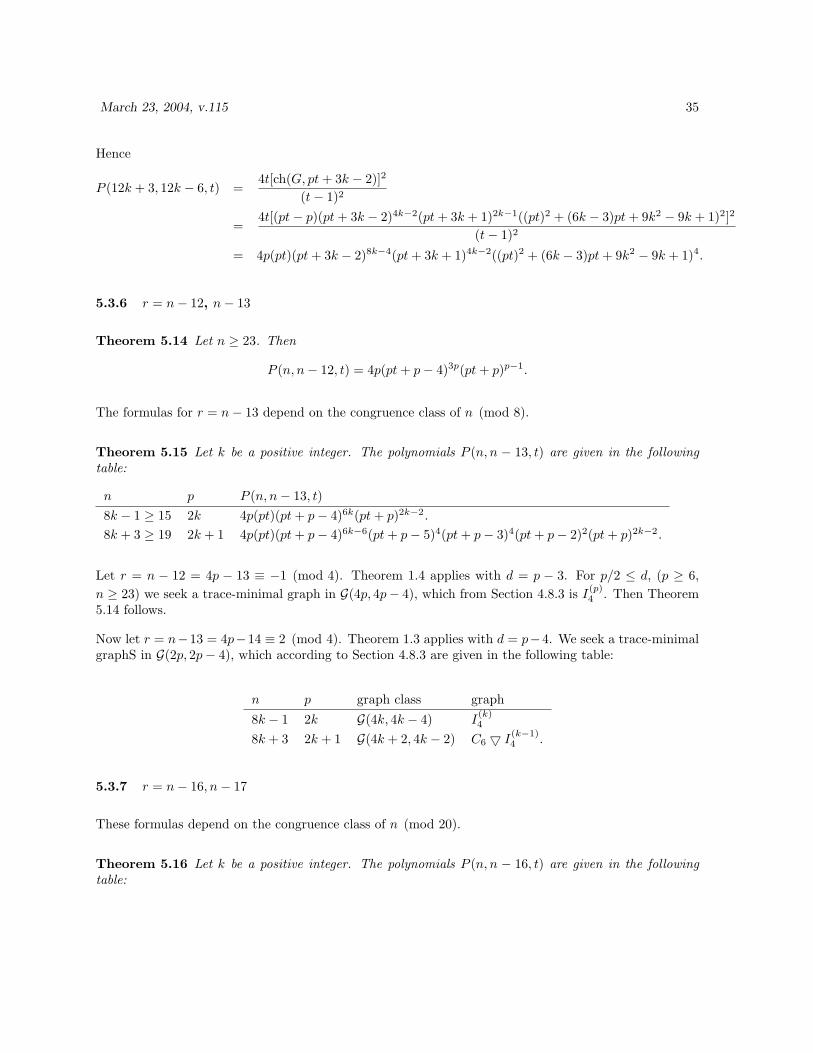
5.3.6 r = n− 12, n− 13

Theorem 5.14 Let n ≥ 23. Then

P (n, n− 12, t) = 4p(pt + p− 4)3p(pt + p)p−1.

The formulas for r = n− 13 depend on the congruence class of n (mod 8).

Theorem 5.15 Let k be a positive integer. The polynomials P (n, n − 13, t) are given in the followingtable:

n p P (n, n− 13, t)8k − 1 ≥ 15 2k 4p(pt)(pt + p− 4)6k(pt + p)2k−2.8k + 3 ≥ 19 2k + 1 4p(pt)(pt + p− 4)6k−6(pt + p− 5)4(pt + p− 3)4(pt + p− 2)2(pt + p)2k−2.

Let r = n − 12 = 4p − 13 ≡ −1 (mod 4). Theorem 1.4 applies with d = p − 3. For p/2 ≤ d, (p ≥ 6,n ≥ 23) we seek a trace-minimal graph in G(4p, 4p− 4), which from Section 4.8.3 is I

(p)4 . Then Theorem

5.14 follows.

Now let r = n−13 = 4p−14 ≡ 2 (mod 4). Theorem 1.3 applies with d = p−4. We seek a trace-minimalgraphS in G(2p, 2p− 4), which according to Section 4.8.3 are given in the following table:

n p graph class graph8k − 1 2k G(4k, 4k − 4) I

(k)4

8k + 3 2k + 1 G(4k + 2, 4k − 2) C6 5 I(k−1)4 .

5.3.7 r = n− 16, n− 17

These formulas depend on the congruence class of n (mod 20).


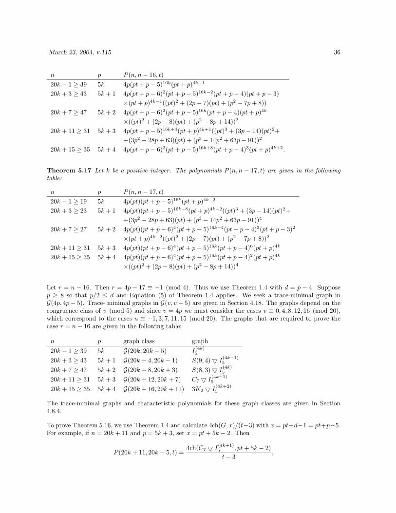
March 23, 2004, v.115 36

n p P (n, n− 16, t)20k − 1 ≥ 39 5k 4p(pt + p− 5)16k(pt + p)4k−1

20k + 3 ≥ 43 5k + 1 4p(pt + p− 6)2(pt + p− 5)16k−2(pt + p− 4)(pt + p− 3)×(pt + p)4k−1((pt)2 + (2p− 7)(pt) + (p2 − 7p + 8))

20k + 7 ≥ 47 5k + 2 4p(pt + p− 6)2(pt + p− 5)16k(pt + p− 4)(pt + p)4k

×((pt)2 + (2p− 8)(pt) + (p2 − 8p + 14))2

20k + 11 ≥ 31 5k + 3 4p(pt + p− 5)16k+4(pt + p)4k+1((pt)3 + (3p− 14)(pt)2++(3p2 − 28p + 63)(pt) + (p3 − 14p2 + 63p− 91))2

20k + 15 ≥ 35 5k + 4 4p(pt + p− 6)2(pt + p− 5)16k+8(pt + p− 4)3(pt + p)4k+2.


n p P (n, n− 17, t)20k − 1 ≥ 19 5k 4p(pt)(pt + p− 5)16k(pt + p)4k−2

20k + 3 ≥ 23 5k + 1 4p(pt)(pt + p− 5)16k−8(pt + p)4k−2((pt)3 + (3p− 14)(pt)2++(3p2 − 28p + 63)(pt) + (p3 − 14p2 + 63p− 91))4

20k + 7 ≥ 27 5k + 2 4p(pt)(pt + p− 6)4(pt + p− 5)16k−4(pt + p− 4)2(pt + p− 3)2

×(pt + p)4k−2((pt)2 + (2p− 7)(pt) + (p2 − 7p + 8))2

20k + 11 ≥ 31 5k + 3 4p(pt)(pt + p− 6)4(pt + p− 5)16k(pt + p− 4)6(pt + p)4k

20k + 15 ≥ 35 5k + 4 4p(pt)(pt + p− 6)4(pt + p− 5)16k(pt + p− 4)2(pt + p)4k

×((pt)2 + (2p− 8)(pt) + (p2 − 8p + 14))4

Let r = n − 16. Then r = 4p − 17 ≡ −1 (mod 4). Thus we use Theorem 1.4 with d = p − 4. Supposep ≥ 8 so that p/2 ≤ d and Equation (5) of Theorem 1.4 applies. We seek a trace-minimal graph inG(4p, 4p− 5). Trace- minimal graphs in G(v, v − 5) are given in Section 4.18. The graphs depend on thecongruence class of v (mod 5) and since v = 4p we must consider the cases v ≡ 0, 4, 8, 12, 16 (mod 20),which correspond to the cases n ≡ −1, 3, 7, 11, 15 (mod 20). The graphs that are required to prove thecase r = n− 16 are given in the following table:


(4k)5

20k + 3 ≥ 43 5k + 1 G(20k + 4, 20k − 1) S(9, 4)5 I(4k−1)5

20k + 7 ≥ 47 5k + 2 G(20k + 8, 20k + 3) S(8, 3)5 I(4k)5

20k + 11 ≥ 31 5k + 3 G(20k + 12, 20k + 7) C7 5 I(4k+1)5

20k + 15 ≥ 35 5k + 4 G(20k + 16, 20k + 11) 3K2 5 I(4k+2)5

The trace-minimal graphs and characteristic polynomials for these graph classes are given in Section4.8.4.

To prove Theorem 5.16, we use Theorem 1.4 and calculate 4ch(G, x)/(t−3) with x = pt+d−1 = pt+p−5.For example, if n = 20k + 11 and p = 5k + 3, set x = pt + 5k − 2. Then

P (20k + 11, 20k − 5, t) =4ch(C7 5 I

(4k+1)5 , pt + 5k − 2)

t− 3,

March 23, 2004, v.115 37

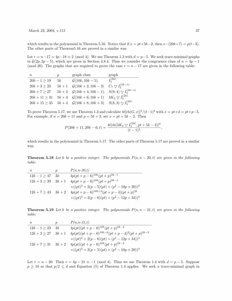
which results in the polynomial in Theorem 5.16. Notice that if x = pt+5k−2, then x−(20k+7) = p(t−3).The other parts of Theorem5.16 are proved in a similar way.

Let r = n−17 = 4p−18 ≡ 2 (mod 4). We use Theorem 1.3 with d = p−5. We seek trace-minimal graphsin G(2p, 2p − 5), which are given in Section 4.8.4. Thus we consider the congruence class of n = 4p − 1(mod 20). The graphs that are required to prove the case r = n− 17 are given in the following table:


(2k)5

20k + 3 ≥ 23 5k + 1 G(10k + 2, 10k − 3) C7 5 I(2k−1)5

20k + 7 ≥ 27 5k + 2 G(10k + 4, 10k − 1) S(9, 4)5 I(2k−1)5

20k + 11 ≥ 31 5k + 3 G(10k + 6, 10k + 1) 3K2 5 I(2k)5

20k + 15 ≥ 35 5k + 4 G(10k + 8, 10k + 3) S(8, 3)5 I(2k)5

To prove Theorem 5.17, we use Theorem 1.3 and calculate 4t[ch(G, x)]2/(t−1)2 with x = pt+d = pt+p−5.For example, if n = 20k + 11 and p = 5k + 3, set x = pt + 5k − 2. Then

P (20k + 11, 20k − 6, t) =4t[ch(3K2 5 I

(2k)5 , pt + 5k − 2)]2

(t− 1)2,

which results in the polynomial in Theorem 5.17. The other parts of Theorem 5.17 are proved in a similarway.


n p P(n,n-20,t)12k − 1 ≥ 47 3k 4p(pt + p− 6)10k(pt + p)2k−1

12k + 3 ≥ 39 3k + 1 4p(pt + p− 6)10k(pt + p)2k−1

×((pt)2 + 2(p− 5)(pt) + (p2 − 10p + 20))2

12k + 7 ≥ 43 3k + 2 4p(pt + p− 6)10k+2(pt + p− 4)(pt + p)2k

×((pt)2 + 2(p− 6)(pt) + (p2 − 12p + 34))2


n p P(n,n-21,t)12k − 1 ≥ 23 3k 4p(pt)(pt + p− 6)10k(pt + p)2k−2

12k + 3 ≥ 27 3k + 1 4p(pt)(pt + p− 6)10k−6(pt + p− 4)2(pt + p)2k−2

×((pt)2 + 2(p− 6)(pt) + (p2 − 12p + 34))4

12k + 7 ≥ 31 3k + 2 4p(pt)(pt + p− 6)10k(pt + p)2k−2

×((pt)2 + 2(p− 5)(pt) + (p2 − 10p + 20))4

Let r = n − 20. Then r = 4p − 21 ≡ −1 (mod 4). Thus we use Theorem 1.4 with d = p − 5. Supposep ≥ 10 so that p/2 ≤ d and Equation (5) of Theorem 1.4 applies. We seek a trace-minimal graph in

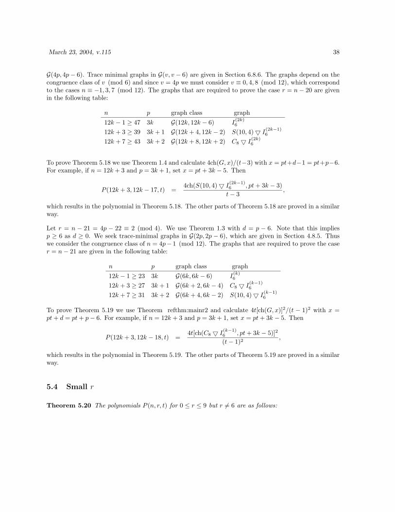
March 23, 2004, v.115 38

G(4p, 4p− 6). Trace minimal graphs in G(v, v − 6) are given in Section 6.8.6. The graphs depend on thecongruence class of v (mod 6) and since v = 4p we must consider v ≡ 0, 4, 8 (mod 12), which correspondto the cases n ≡ −1, 3, 7 (mod 12). The graphs that are required to prove the case r = n− 20 are givenin the following table:


(2k)6

12k + 3 ≥ 39 3k + 1 G(12k + 4, 12k − 2) S(10, 4)5 I(2k−1)6

12k + 7 ≥ 43 3k + 2 G(12k + 8, 12k + 2) C8 5 I(2k)6

To prove Theorem 5.18 we use Theorem 1.4 and calculate 4ch(G, x)/(t−3) with x = pt+d−1 = pt+p−6.For example, if n = 12k + 3 and p = 3k + 1, set x = pt + 3k − 5. Then

P (12k + 3, 12k − 17, t) =4ch(S(10, 4)5 I

(2k−1)6 , pt + 3k − 3)

t− 3,


Let r = n − 21 = 4p − 22 ≡ 2 (mod 4). We use Theorem 1.3 with d = p − 6. Note that this impliesp ≥ 6 as d ≥ 0. We seek trace-minimal graphs in G(2p, 2p − 6), which are given in Section 4.8.5. Thuswe consider the congruence class of n = 4p− 1 (mod 12). The graphs that are required to prove the caser = n− 21 are given in the following table:


(k)6

12k + 3 ≥ 27 3k + 1 G(6k + 2, 6k − 4) C8 5 I(k−1)6

12k + 7 ≥ 31 3k + 2 G(6k + 4, 6k − 2) S(10, 4)5 I(k−1)6

To prove Theorem 5.19 we use Theorem refthm:mainr2 and calculate 4t[ch(G, x)]2/(t − 1)2 with x =pt + d = pt + p− 6. For example, if n = 12k + 3 and p = 3k + 1, set x = pt + 3k − 5. Then

P (12k + 3, 12k − 18, t) =4t[ch(C8 5 I

(k−1)6 , pt + 3k − 5)]2

(t− 1)2,


5.4 Small r

Theorem 5.20 The polynomials P (n, r, t) for 0 ≤ r ≤ 9 but r 6= 6 are as follows:

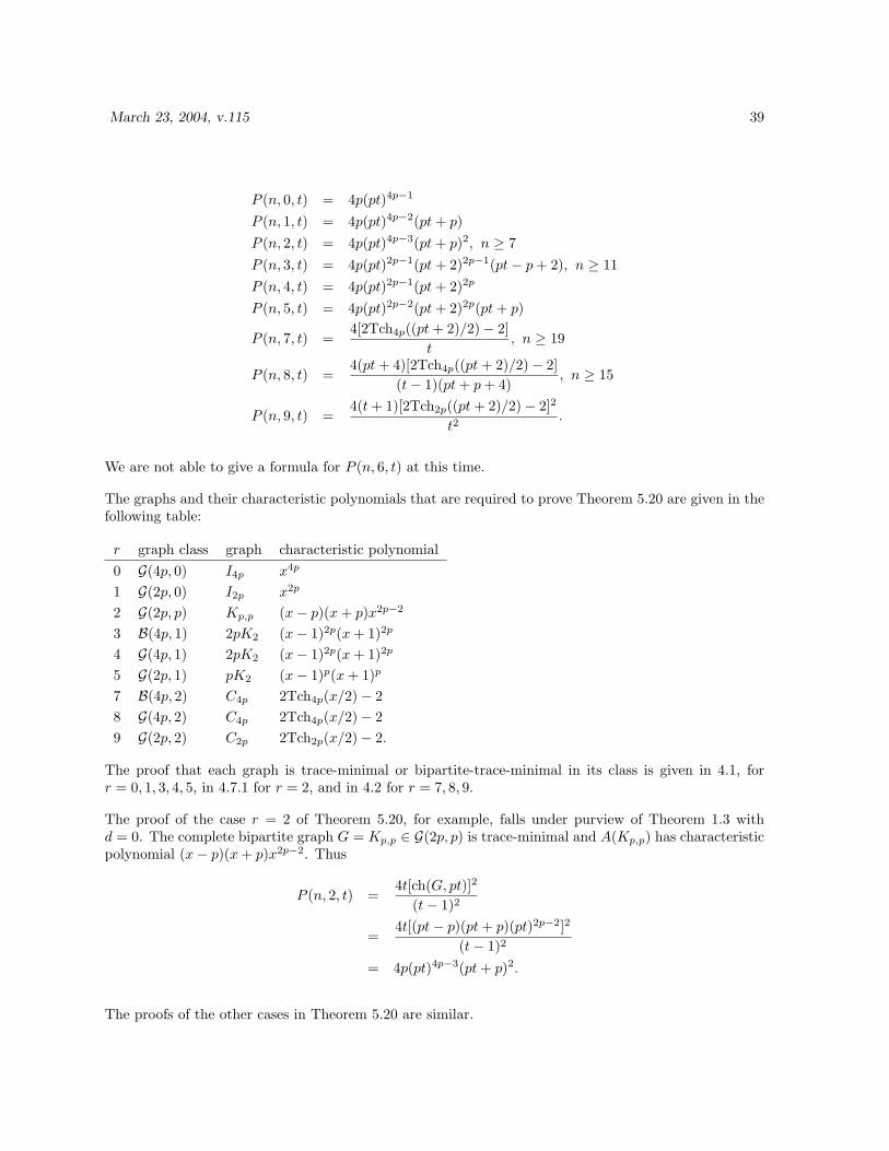
March 23, 2004, v.115 39

P (n, 0, t) = 4p(pt)4p−1

P (n, 1, t) = 4p(pt)4p−2(pt + p)P (n, 2, t) = 4p(pt)4p−3(pt + p)2, n ≥ 7P (n, 3, t) = 4p(pt)2p−1(pt + 2)2p−1(pt− p + 2), n ≥ 11P (n, 4, t) = 4p(pt)2p−1(pt + 2)2p

P (n, 5, t) = 4p(pt)2p−2(pt + 2)2p(pt + p)

P (n, 7, t) =4[2Tch4p((pt + 2)/2)− 2]

t, n ≥ 19

P (n, 8, t) =4(pt + 4)[2Tch4p((pt + 2)/2)− 2]

(t− 1)(pt + p + 4), n ≥ 15

P (n, 9, t) =4(t + 1)[2Tch2p((pt + 2)/2)− 2]2

t2.

We are not able to give a formula for P (n, 6, t) at this time.

The graphs and their characteristic polynomials that are required to prove Theorem 5.20 are given in thefollowing table:

r graph class graph characteristic polynomial0 G(4p, 0) I4p x4p

1 G(2p, 0) I2p x2p

2 G(2p, p) Kp,p (x− p)(x + p)x2p−2

3 B(4p, 1) 2pK2 (x− 1)2p(x + 1)2p

4 G(4p, 1) 2pK2 (x− 1)2p(x + 1)2p

5 G(2p, 1) pK2 (x− 1)p(x + 1)p

7 B(4p, 2) C4p 2Tch4p(x/2)− 28 G(4p, 2) C4p 2Tch4p(x/2)− 29 G(2p, 2) C2p 2Tch2p(x/2)− 2.

The proof that each graph is trace-minimal or bipartite-trace-minimal in its class is given in 4.1, forr = 0, 1, 3, 4, 5, in 4.7.1 for r = 2, and in 4.2 for r = 7, 8, 9.

The proof of the case r = 2 of Theorem 5.20, for example, falls under purview of Theorem 1.3 withd = 0. The complete bipartite graph G = Kp,p ∈ G(2p, p) is trace-minimal and A(Kp,p) has characteristicpolynomial (x− p)(x + p)x2p−2. Thus

P (n, 2, t) =4t[ch(G, pt)]2

(t− 1)2

=4t[(pt− p)(pt + p)(pt)2p−2]2

(t− 1)2

= 4p(pt)4p−3(pt + p)2.

The proofs of the other cases in Theorem 5.20 are similar.

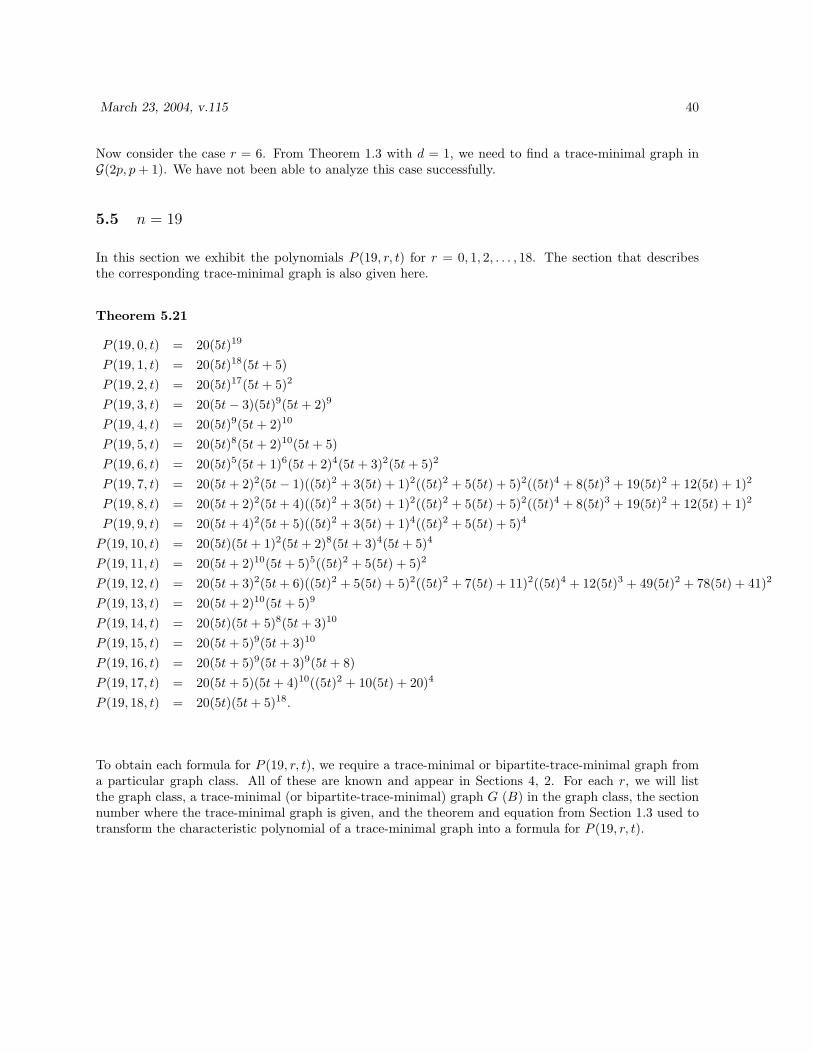
March 23, 2004, v.115 40

Now consider the case r = 6. From Theorem 1.3 with d = 1, we need to find a trace-minimal graph inG(2p, p + 1). We have not been able to analyze this case successfully.

5.5 n = 19

In this section we exhibit the polynomials P (19, r, t) for r = 0, 1, 2, . . . , 18. The section that describesthe corresponding trace-minimal graph is also given here.

Theorem 5.21

P (19, 0, t) = 20(5t)19

P (19, 1, t) = 20(5t)18(5t + 5)P (19, 2, t) = 20(5t)17(5t + 5)2

P (19, 3, t) = 20(5t− 3)(5t)9(5t + 2)9

P (19, 4, t) = 20(5t)9(5t + 2)10

P (19, 5, t) = 20(5t)8(5t + 2)10(5t + 5)P (19, 6, t) = 20(5t)5(5t + 1)6(5t + 2)4(5t + 3)2(5t + 5)2

P (19, 7, t) = 20(5t + 2)2(5t− 1)((5t)2 + 3(5t) + 1)2((5t)2 + 5(5t) + 5)2((5t)4 + 8(5t)3 + 19(5t)2 + 12(5t) + 1)2

P (19, 8, t) = 20(5t + 2)2(5t + 4)((5t)2 + 3(5t) + 1)2((5t)2 + 5(5t) + 5)2((5t)4 + 8(5t)3 + 19(5t)2 + 12(5t) + 1)2

P (19, 9, t) = 20(5t + 4)2(5t + 5)((5t)2 + 3(5t) + 1)4((5t)2 + 5(5t) + 5)4

P (19, 10, t) = 20(5t)(5t + 1)2(5t + 2)8(5t + 3)4(5t + 5)4

P (19, 11, t) = 20(5t + 2)10(5t + 5)5((5t)2 + 5(5t) + 5)2

P (19, 12, t) = 20(5t + 3)2(5t + 6)((5t)2 + 5(5t) + 5)2((5t)2 + 7(5t) + 11)2((5t)4 + 12(5t)3 + 49(5t)2 + 78(5t) + 41)2

P (19, 13, t) = 20(5t + 2)10(5t + 5)9

P (19, 14, t) = 20(5t)(5t + 5)8(5t + 3)10

P (19, 15, t) = 20(5t + 5)9(5t + 3)10

P (19, 16, t) = 20(5t + 5)9(5t + 3)9(5t + 8)P (19, 17, t) = 20(5t + 5)(5t + 4)10((5t)2 + 10(5t) + 20)4

P (19, 18, t) = 20(5t)(5t + 5)18.

To obtain each formula for P (19, r, t), we require a trace-minimal or bipartite-trace-minimal graph froma particular graph class. All of these are known and appear in Sections 4, 2. For each r, we will listthe graph class, a trace-minimal (or bipartite-trace-minimal) graph G (B) in the graph class, the sectionnumber where the trace-minimal graph is given, and the theorem and equation from Section 1.3 used totransform the characteristic polynomial of a trace-minimal graph into a formula for P (19, r, t).

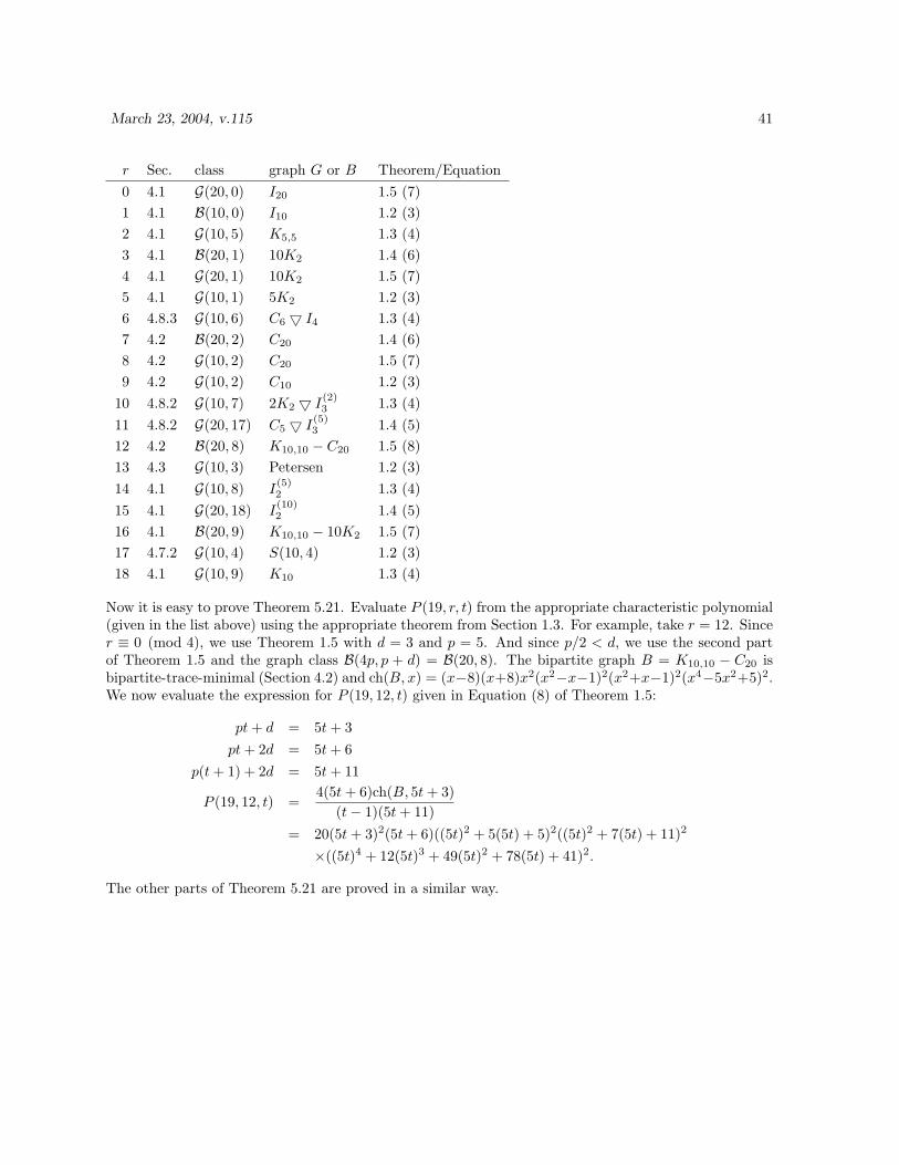
March 23, 2004, v.115 41

r Sec. class graph G or B Theorem/Equation0 4.1 G(20, 0) I20 1.5 (7)1 4.1 B(10, 0) I10 1.2 (3)2 4.1 G(10, 5) K5,5 1.3 (4)3 4.1 B(20, 1) 10K2 1.4 (6)4 4.1 G(20, 1) 10K2 1.5 (7)5 4.1 G(10, 1) 5K2 1.2 (3)6 4.8.3 G(10, 6) C6 5 I4 1.3 (4)7 4.2 B(20, 2) C20 1.4 (6)8 4.2 G(10, 2) C20 1.5 (7)9 4.2 G(10, 2) C10 1.2 (3)

10 4.8.2 G(10, 7) 2K2 5 I(2)3 1.3 (4)

11 4.8.2 G(20, 17) C5 5 I(5)3 1.4 (5)

12 4.2 B(20, 8) K10,10 − C20 1.5 (8)13 4.3 G(10, 3) Petersen 1.2 (3)14 4.1 G(10, 8) I

(5)2 1.3 (4)

15 4.1 G(20, 18) I(10)2 1.4 (5)

16 4.1 B(20, 9) K10,10 − 10K2 1.5 (7)17 4.7.2 G(10, 4) S(10, 4) 1.2 (3)18 4.1 G(10, 9) K10 1.3 (4)

Now it is easy to prove Theorem 5.21. Evaluate P (19, r, t) from the appropriate characteristic polynomial(given in the list above) using the appropriate theorem from Section 1.3. For example, take r = 12. Sincer ≡ 0 (mod 4), we use Theorem 1.5 with d = 3 and p = 5. And since p/2 < d, we use the second partof Theorem 1.5 and the graph class B(4p, p + d) = B(20, 8). The bipartite graph B = K10,10 − C20 isbipartite-trace-minimal (Section 4.2) and ch(B, x) = (x−8)(x+8)x2(x2−x−1)2(x2+x−1)2(x4−5x2+5)2.We now evaluate the expression for P (19, 12, t) given in Equation (8) of Theorem 1.5:

pt + d = 5t + 3pt + 2d = 5t + 6

p(t + 1) + 2d = 5t + 11

P (19, 12, t) =4(5t + 6)ch(B, 5t + 3)

(t− 1)(5t + 11)= 20(5t + 3)2(5t + 6)((5t)2 + 5(5t) + 5)2((5t)2 + 7(5t) + 11)2

×((5t)4 + 12(5t)3 + 49(5t)2 + 78(5t) + 41)2.

The other parts of Theorem 5.21 are proved in a similar way.

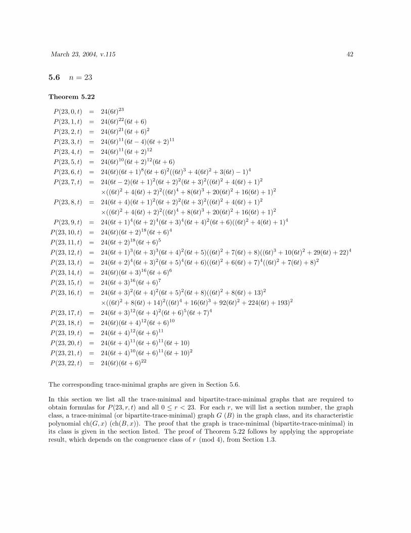
March 23, 2004, v.115 42

5.6 n = 23

Theorem 5.22

P (23, 0, t) = 24(6t)23

P (23, 1, t) = 24(6t)22(6t + 6)P (23, 2, t) = 24(6t)21(6t + 6)2

P (23, 3, t) = 24(6t)11(6t− 4)(6t + 2)11

P (23, 4, t) = 24(6t)11(6t + 2)12

P (23, 5, t) = 24(6t)10(6t + 2)12(6t + 6)P (23, 6, t) = 24(6t)(6t + 1)8(6t + 6)2((6t)3 + 4(6t)2 + 3(6t)− 1)4

P (23, 7, t) = 24(6t− 2)(6t + 1)2(6t + 2)2(6t + 3)2((6t)2 + 4(6t) + 1)2

×((6t)2 + 4(6t) + 2)2((6t)4 + 8(6t)3 + 20(6t)2 + 16(6t) + 1)2

P (23, 8, t) = 24(6t + 4)(6t + 1)2(6t + 2)2(6t + 3)2((6t)2 + 4(6t) + 1)2

×((6t)2 + 4(6t) + 2)2((6t)4 + 8(6t)3 + 20(6t)2 + 16(6t) + 1)2

P (23, 9, t) = 24(6t + 1)4(6t + 2)4(6t + 3)4(6t + 4)2(6t + 6)((6t)2 + 4(6t) + 1)4

P (23, 10, t) = 24(6t)(6t + 2)18(6t + 6)4

P (23, 11, t) = 24(6t + 2)18(6t + 6)5

P (23, 12, t) = 24(6t + 1)3(6t + 3)3(6t + 4)2(6t + 5)((6t)2 + 7(6t) + 8)((6t)3 + 10(6t)2 + 29(6t) + 22)4

P (23, 13, t) = 24(6t + 2)4(6t + 3)2(6t + 5)4(6t + 6)((6t)2 + 6(6t) + 7)4((6t)2 + 7(6t) + 8)2

P (23, 14, t) = 24(6t)(6t + 3)16(6t + 6)6

P (23, 15, t) = 24(6t + 3)16(6t + 6)7

P (23, 16, t) = 24(6t + 3)2(6t + 4)2(6t + 5)2(6t + 8)((6t)2 + 8(6t) + 13)2

×((6t)2 + 8(6t) + 14)2((6t)4 + 16(6t)3 + 92(6t)2 + 224(6t) + 193)2

P (23, 17, t) = 24(6t + 3)12(6t + 4)2(6t + 6)5(6t + 7)4

P (23, 18, t) = 24(6t)(6t + 4)12(6t + 6)10

P (23, 19, t) = 24(6t + 4)12(6t + 6)11

P (23, 20, t) = 24(6t + 4)11(6t + 6)11(6t + 10)P (23, 21, t) = 24(6t + 4)10(6t + 6)11(6t + 10)2

P (23, 22, t) = 24(6t)(6t + 6)22

The corresponding trace-minimal graphs are given in Section 5.6.

In this section we list all the trace-minimal and bipartite-trace-minimal graphs that are required toobtain formulas for P (23, r, t) and all 0 ≤ r < 23. For each r, we will list a section number, the graphclass, a trace-minimal (or bipartite-trace-minimal) graph G (B) in the graph class, and its characteristicpolynomial ch(G, x) (ch(B, x)). The proof that the graph is trace-minimal (bipartite-trace-minimal) inits class is given in the section listed. The proof of Theorem 5.22 follows by applying the appropriateresult, which depends on the congruence class of r (mod 4), from Section 1.3.

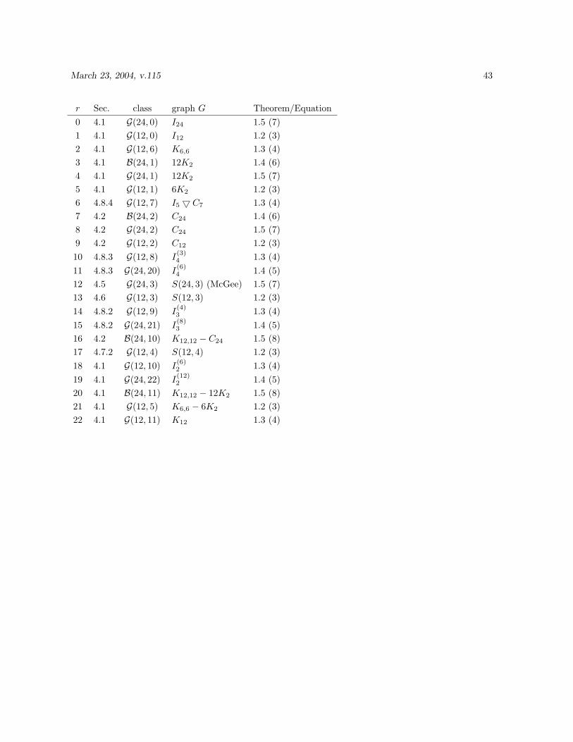
March 23, 2004, v.115 43

r Sec. class graph G Theorem/Equation0 4.1 G(24, 0) I24 1.5 (7)1 4.1 G(12, 0) I12 1.2 (3)2 4.1 G(12, 6) K6,6 1.3 (4)3 4.1 B(24, 1) 12K2 1.4 (6)4 4.1 G(24, 1) 12K2 1.5 (7)5 4.1 G(12, 1) 6K2 1.2 (3)6 4.8.4 G(12, 7) I5 5 C7 1.3 (4)7 4.2 B(24, 2) C24 1.4 (6)8 4.2 G(24, 2) C24 1.5 (7)9 4.2 G(12, 2) C12 1.2 (3)10 4.8.3 G(12, 8) I

(3)4 1.3 (4)

11 4.8.3 G(24, 20) I(6)4 1.4 (5)

12 4.5 G(24, 3) S(24, 3) (McGee) 1.5 (7)13 4.6 G(12, 3) S(12, 3) 1.2 (3)14 4.8.2 G(12, 9) I

(4)3 1.3 (4)

15 4.8.2 G(24, 21) I(8)3 1.4 (5)

16 4.2 B(24, 10) K12,12 − C24 1.5 (8)17 4.7.2 G(12, 4) S(12, 4) 1.2 (3)18 4.1 G(12, 10) I

(6)2 1.3 (4)

19 4.1 G(24, 22) I(12)2 1.4 (5)

20 4.1 B(24, 11) K12,12 − 12K2 1.5 (8)21 4.1 G(12, 5) K6,6 − 6K2 1.2 (3)22 4.1 G(12, 11) K12 1.3 (4)

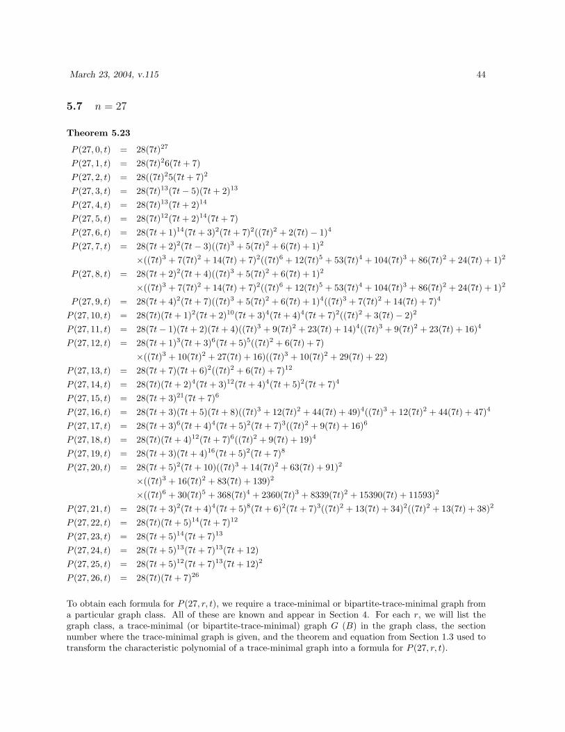
March 23, 2004, v.115 44

5.7 n = 27

Theorem 5.23

P (27, 0, t) = 28(7t)27

P (27, 1, t) = 28(7t)26(7t + 7)P (27, 2, t) = 28((7t)25(7t + 7)2

P (27, 3, t) = 28(7t)13(7t− 5)(7t + 2)13

P (27, 4, t) = 28(7t)13(7t + 2)14

P (27, 5, t) = 28(7t)12(7t + 2)14(7t + 7)P (27, 6, t) = 28(7t + 1)14(7t + 3)2(7t + 7)2((7t)2 + 2(7t)− 1)4

P (27, 7, t) = 28(7t + 2)2(7t− 3)((7t)3 + 5(7t)2 + 6(7t) + 1)2

×((7t)3 + 7(7t)2 + 14(7t) + 7)2((7t)6 + 12(7t)5 + 53(7t)4 + 104(7t)3 + 86(7t)2 + 24(7t) + 1)2

P (27, 8, t) = 28(7t + 2)2(7t + 4)((7t)3 + 5(7t)2 + 6(7t) + 1)2

×((7t)3 + 7(7t)2 + 14(7t) + 7)2((7t)6 + 12(7t)5 + 53(7t)4 + 104(7t)3 + 86(7t)2 + 24(7t) + 1)2

P (27, 9, t) = 28(7t + 4)2(7t + 7)((7t)3 + 5(7t)2 + 6(7t) + 1)4((7t)3 + 7(7t)2 + 14(7t) + 7)4

P (27, 10, t) = 28(7t)(7t + 1)2(7t + 2)10(7t + 3)4(7t + 4)4(7t + 7)2((7t)2 + 3(7t)− 2)2

P (27, 11, t) = 28(7t− 1)(7t + 2)(7t + 4)((7t)3 + 9(7t)2 + 23(7t) + 14)4((7t)3 + 9(7t)2 + 23(7t) + 16)4

P (27, 12, t) = 28(7t + 1)3(7t + 3)6(7t + 5)5((7t)2 + 6(7t) + 7)×((7t)3 + 10(7t)2 + 27(7t) + 16)((7t)3 + 10(7t)2 + 29(7t) + 22)

P (27, 13, t) = 28(7t + 7)(7t + 6)2((7t)2 + 6(7t) + 7)12

P (27, 14, t) = 28(7t)(7t + 2)4(7t + 3)12(7t + 4)4(7t + 5)2(7t + 7)4

P (27, 15, t) = 28(7t + 3)21(7t + 7)6

P (27, 16, t) = 28(7t + 3)(7t + 5)(7t + 8)((7t)3 + 12(7t)2 + 44(7t) + 49)4((7t)3 + 12(7t)2 + 44(7t) + 47)4

P (27, 17, t) = 28(7t + 3)6(7t + 4)4(7t + 5)2(7t + 7)3((7t)2 + 9(7t) + 16)6

P (27, 18, t) = 28(7t)(7t + 4)12(7t + 7)6((7t)2 + 9(7t) + 19)4

P (27, 19, t) = 28(7t + 3)(7t + 4)16(7t + 5)2(7t + 7)8

P (27, 20, t) = 28(7t + 5)2(7t + 10)((7t)3 + 14(7t)2 + 63(7t) + 91)2

×((7t)3 + 16(7t)2 + 83(7t) + 139)2

×((7t)6 + 30(7t)5 + 368(7t)4 + 2360(7t)3 + 8339(7t)2 + 15390(7t) + 11593)2

P (27, 21, t) = 28(7t + 3)2(7t + 4)4(7t + 5)8(7t + 6)2(7t + 7)3((7t)2 + 13(7t) + 34)2((7t)2 + 13(7t) + 38)2

P (27, 22, t) = 28(7t)(7t + 5)14(7t + 7)12

P (27, 23, t) = 28(7t + 5)14(7t + 7)13

P (27, 24, t) = 28(7t + 5)13(7t + 7)13(7t + 12)P (27, 25, t) = 28(7t + 5)12(7t + 7)13(7t + 12)2

P (27, 26, t) = 28(7t)(7t + 7)26

To obtain each formula for P (27, r, t), we require a trace-minimal or bipartite-trace-minimal graph froma particular graph class. All of these are known and appear in Section 4. For each r, we will list thegraph class, a trace-minimal (or bipartite-trace-minimal) graph G (B) in the graph class, the sectionnumber where the trace-minimal graph is given, and the theorem and equation from Section 1.3 used totransform the characteristic polynomial of a trace-minimal graph into a formula for P (27, r, t).

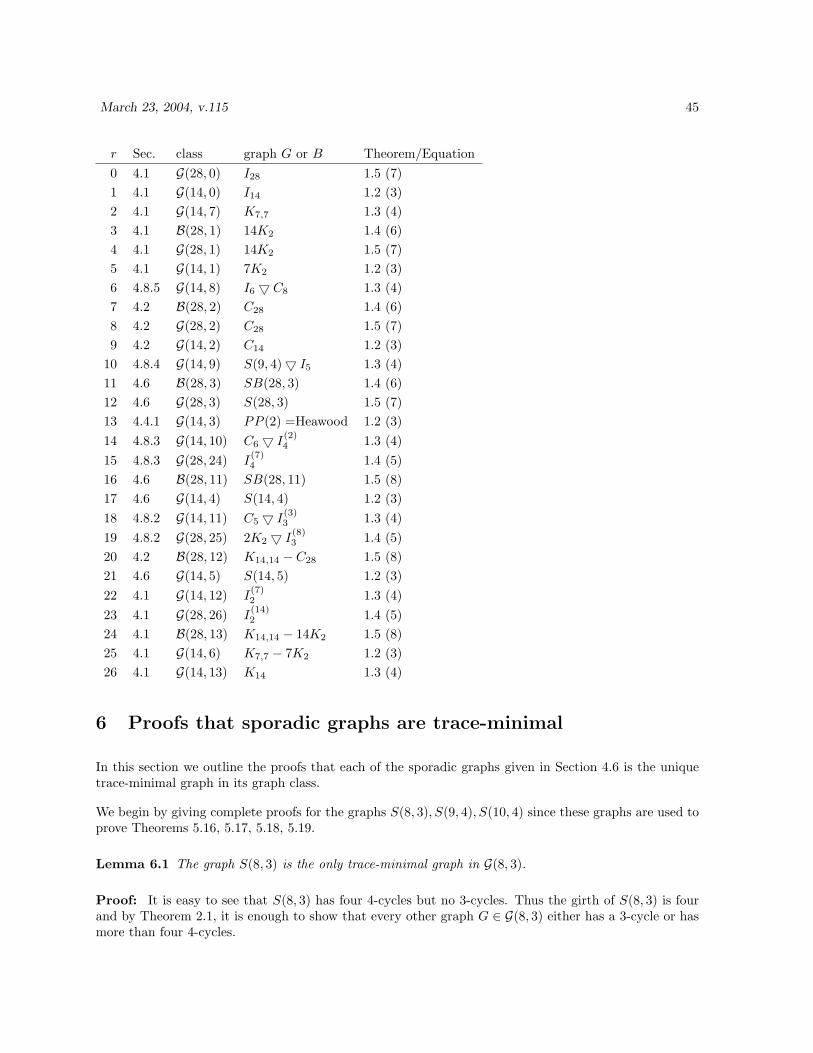
March 23, 2004, v.115 45

r Sec. class graph G or B Theorem/Equation0 4.1 G(28, 0) I28 1.5 (7)1 4.1 G(14, 0) I14 1.2 (3)2 4.1 G(14, 7) K7,7 1.3 (4)3 4.1 B(28, 1) 14K2 1.4 (6)4 4.1 G(28, 1) 14K2 1.5 (7)5 4.1 G(14, 1) 7K2 1.2 (3)6 4.8.5 G(14, 8) I6 5 C8 1.3 (4)7 4.2 B(28, 2) C28 1.4 (6)8 4.2 G(28, 2) C28 1.5 (7)9 4.2 G(14, 2) C14 1.2 (3)

10 4.8.4 G(14, 9) S(9, 4)5 I5 1.3 (4)11 4.6 B(28, 3) SB(28, 3) 1.4 (6)12 4.6 G(28, 3) S(28, 3) 1.5 (7)13 4.4.1 G(14, 3) PP (2) =Heawood 1.2 (3)14 4.8.3 G(14, 10) C6 5 I

(2)4 1.3 (4)

15 4.8.3 G(28, 24) I(7)4 1.4 (5)

16 4.6 B(28, 11) SB(28, 11) 1.5 (8)17 4.6 G(14, 4) S(14, 4) 1.2 (3)18 4.8.2 G(14, 11) C5 5 I

(3)3 1.3 (4)

19 4.8.2 G(28, 25) 2K2 5 I(8)3 1.4 (5)

20 4.2 B(28, 12) K14,14 − C28 1.5 (8)21 4.6 G(14, 5) S(14, 5) 1.2 (3)22 4.1 G(14, 12) I

(7)2 1.3 (4)

23 4.1 G(28, 26) I(14)2 1.4 (5)

24 4.1 B(28, 13) K14,14 − 14K2 1.5 (8)25 4.1 G(14, 6) K7,7 − 7K2 1.2 (3)26 4.1 G(14, 13) K14 1.3 (4)

6 Proofs that sporadic graphs are trace-minimal

In this section we outline the proofs that each of the sporadic graphs given in Section 4.6 is the uniquetrace-minimal graph in its graph class.

We begin by giving complete proofs for the graphs S(8, 3), S(9, 4), S(10, 4) since these graphs are used toprove Theorems 5.16, 5.17, 5.18, 5.19.

Lemma 6.1 The graph S(8, 3) is the only trace-minimal graph in G(8, 3).

Proof: It is easy to see that S(8, 3) has four 4-cycles but no 3-cycles. Thus the girth of S(8, 3) is fourand by Theorem 2.1, it is enough to show that every other graph G ∈ G(8, 3) either has a 3-cycle or hasmore than four 4-cycles.

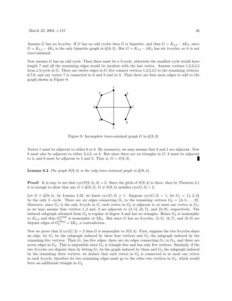
March 23, 2004, v.115 46

Assume G has no 3-cycles. If G has no odd cycles then G is bipartite, and thus G = K4,4 − 4K2, sinceG = K4,4 − 4K2 is the only bipartite graph in G(8, 3). But G = K4,4 − 4K2 has six 4-cycles, so it is nottrace-minimal.

Now assume G has an odd cycle. Then there must be a 5-cycle, otherwise the smallest cycle would havelength 7 and all the remaining edges would be incident with the last vertex. Assume vertices 1,2,3,4,5form a 5-cycle in G. There are twelve edges in G; five connect vertices 1,2,3,4,5 to the remaining vertices,6,7,8; and say vertex 7 is connected to 6 and 8 and to 3. Thus there are four more edges to add to thegraph shown in Figure 8.

1

2

3

4

5

6

7

8

Figure 8: Incomplete trace-minimal graph G in G(8, 3)

Vertex 1 must be adjacent to either 6 or 8. By symmetry, we may assume that 8 and 1 are adjacent. Now8 must also be adjacent to either 2,4,5, or 6. But since there are no triangles in G, 8 must be adjacentto 4, and 6 must be adjacent to 5 and 2. That is, G = S(8, 3).


Proof: It is easy to see that cyc(S(9, 4), 3) = 2. Since the girth of S(9, 4) is three, then by Theorem 2.1it is enough to show that any G ∈ G(9, 4), G 6= S(9, 4) satisfies cyc(G, 3) > 2.

Let G ∈ G(9, 4), by Lemma 4.22, we know cyc(G, 3) ≥ 1. Suppose cyc(G, 3) = 1, let G1 = {1, 2, 3}be the only 3 -cycle. There are six edges connecting G1 to the remaining vertices G2 = {4, 5, . . . , 9}.Moreover, since G1 is the only 3-cycle in G, each vertex in G2 is adjacent to at most one vertex in G1;so we may assume that vertices 1, 2 and, 3 are adjacent to {4, 5}, {6, 7}, and {8, 9}, respectively. Theinduced subgraph obtained from G2 is regular of degree 3 and has no triangles. Hence G2 is isomorphicto K3,3 and thus Gcomp

2 is isomorphic to 2K3. But since G has no 3-cycles, (4, 5), (6, 7), and (8, 9) aredisjoint edges of Gcomp

2 = 2K3, a contradiction.

Now we prove that if cyc(G, 3) = 2 then G is isomorphic to S(9, 4). First, suppose the two 3-cycles sharean edge, let G1 be the subgraph induced by these four vertices and G2 the subgraph induced by theremaining five vertices. Then G1 has five edges, there are six edges connecting G1 to G2, and there areseven edges in G2. This is impossible since G2 is triangle free and has only five vertices. Similarly, if thetwo 3-cycles are disjoint then by letting G1 be the graph induced by them and G2 the subgraph inducedby the remaining three vertices, we deduce that each vertex in G2 is connected to at most one vertexin each 3-cycle, therefore its two remaining edges must go to the other two vertices in G2, which wouldforce an additional triangle in G2.

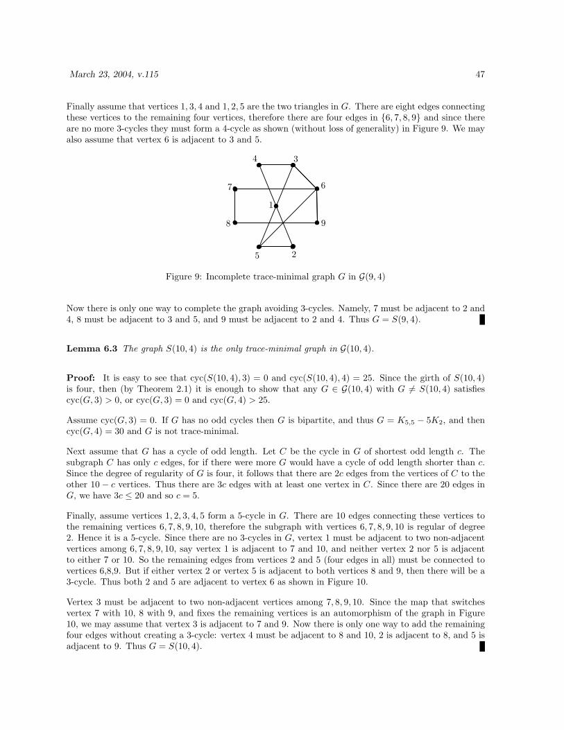
March 23, 2004, v.115 47

Finally assume that vertices 1, 3, 4 and 1, 2, 5 are the two triangles in G. There are eight edges connectingthese vertices to the remaining four vertices, therefore there are four edges in {6, 7, 8, 9} and since thereare no more 3-cycles they must form a 4-cycle as shown (without loss of generality) in Figure 9. We mayalso assume that vertex 6 is adjacent to 3 and 5.

1

2

34

5

67

8 9


Now there is only one way to complete the graph avoiding 3-cycles. Namely, 7 must be adjacent to 2 and4, 8 must be adjacent to 3 and 5, and 9 must be adjacent to 2 and 4. Thus G = S(9, 4).


Proof: It is easy to see that cyc(S(10, 4), 3) = 0 and cyc(S(10, 4), 4) = 25. Since the girth of S(10, 4)is four, then (by Theorem 2.1) it is enough to show that any G ∈ G(10, 4) with G 6= S(10, 4) satisfiescyc(G, 3) > 0, or cyc(G, 3) = 0 and cyc(G, 4) > 25.

Assume cyc(G, 3) = 0. If G has no odd cycles then G is bipartite, and thus G = K5,5 − 5K2, and thencyc(G, 4) = 30 and G is not trace-minimal.

Next assume that G has a cycle of odd length. Let C be the cycle in G of shortest odd length c. Thesubgraph C has only c edges, for if there were more G would have a cycle of odd length shorter than c.Since the degree of regularity of G is four, it follows that there are 2c edges from the vertices of C to theother 10− c vertices. Thus there are 3c edges with at least one vertex in C. Since there are 20 edges inG, we have 3c ≤ 20 and so c = 5.

Finally, assume vertices 1, 2, 3, 4, 5 form a 5-cycle in G. There are 10 edges connecting these vertices tothe remaining vertices 6, 7, 8, 9, 10, therefore the subgraph with vertices 6, 7, 8, 9, 10 is regular of degree2. Hence it is a 5-cycle. Since there are no 3-cycles in G, vertex 1 must be adjacent to two non-adjacentvertices among 6, 7, 8, 9, 10, say vertex 1 is adjacent to 7 and 10, and neither vertex 2 nor 5 is adjacentto either 7 or 10. So the remaining edges from vertices 2 and 5 (four edges in all) must be connected tovertices 6,8,9. But if either vertex 2 or vertex 5 is adjacent to both vertices 8 and 9, then there will be a3-cycle. Thus both 2 and 5 are adjacent to vertex 6 as shown in Figure 10.

Vertex 3 must be adjacent to two non-adjacent vertices among 7, 8, 9, 10. Since the map that switchesvertex 7 with 10, 8 with 9, and fixes the remaining vertices is an automorphism of the graph in Figure10, we may assume that vertex 3 is adjacent to 7 and 9. Now there is only one way to add the remainingfour edges without creating a 3-cycle: vertex 4 must be adjacent to 8 and 10, 2 is adjacent to 8, and 5 isadjacent to 9. Thus G = S(10, 4).

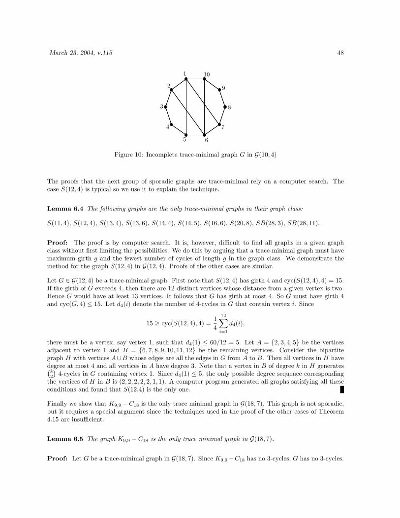
March 23, 2004, v.115 48

1

2

3

4

5 6

7

8

9

10


The proofs that the next group of sporadic graphs are trace-minimal rely on a computer search. Thecase S(12, 4) is typical so we use it to explain the technique.

Lemma 6.4 The following graphs are the only trace-minimal graphs in their graph class:

S(11, 4), S(12, 4), S(13, 4), S(13, 6), S(14, 4), S(14, 5), S(16, 6), S(20, 8), SB(28, 3), SB(28, 11).

Proof: The proof is by computer search. It is, however, difficult to find all graphs in a given graphclass without first limiting the possibilities. We do this by arguing that a trace-minimal graph must havemaximum girth g and the fewest number of cycles of length g in the graph class. We demonstrate themethod for the graph S(12, 4) in G(12, 4). Proofs of the other cases are similar.

Let G ∈ G(12, 4) be a trace-minimal graph. First note that S(12, 4) has girth 4 and cyc(S(12, 4), 4) = 15.If the girth of G exceeds 4, then there are 12 distinct vertices whose distance from a given vertex is two.Hence G would have at least 13 vertices. It follows that G has girth at most 4. So G must have girth 4and cyc(G, 4) ≤ 15. Let d4(i) denote the number of 4-cycles in G that contain vertex i. Since

15 ≥ cyc(S(12, 4), 4) =14

12∑i=1

d4(i),

there must be a vertex, say vertex 1, such that d4(1) ≤ 60/12 = 5. Let A = {2, 3, 4, 5} be the verticesadjacent to vertex 1 and B = {6, 7, 8, 9, 10, 11, 12} be the remaining vertices. Consider the bipartitegraph H with vertices A∪B whose edges are all the edges in G from A to B. Then all vertices in H havedegree at most 4 and all vertices in A have degree 3. Note that a vertex in B of degree k in H generates(k2

)4-cycles in G containing vertex 1. Since d4(1) ≤ 5, the only possible degree sequence corresponding

the vertices of H in B is (2, 2, 2, 2, 2, 1, 1). A computer program generated all graphs satisfying all theseconditions and found that S(12.4) is the only one.

Finally we show that K9,9 −C18 is the only trace minimal graph in G(18, 7). This graph is not sporadic,but it requires a special argument since the techniques used in the proof of the other cases of Theorem4.15 are insufficient.

Lemma 6.5 The graph K9,9 − C18 is the only trace minimal graph in G(18, 7).

Proof: Let G be a trace-minimal graph in G(18, 7). Since K9,9−C18 has no 3-cycles, G has no 3-cycles.

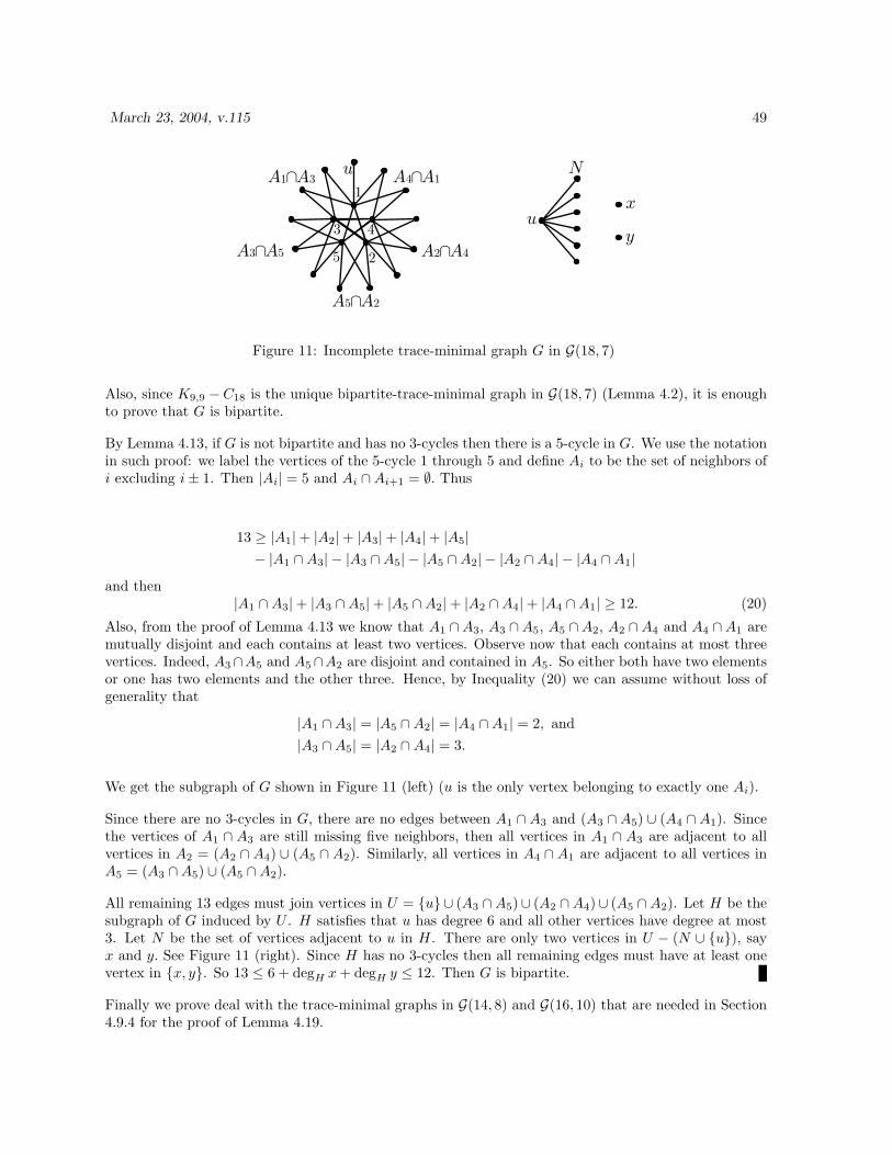
March 23, 2004, v.115 49


Also, since K9,9 − C18 is the unique bipartite-trace-minimal graph in G(18, 7) (Lemma 4.2), it is enoughto prove that G is bipartite.

By Lemma 4.13, if G is not bipartite and has no 3-cycles then there is a 5-cycle in G. We use the notationin such proof: we label the vertices of the 5-cycle 1 through 5 and define Ai to be the set of neighbors ofi excluding i± 1. Then |Ai| = 5 and Ai ∩Ai+1 = ∅. Thus

13 ≥ |A1|+ |A2|+ |A3|+ |A4|+ |A5|− |A1 ∩A3| − |A3 ∩A5| − |A5 ∩A2| − |A2 ∩A4| − |A4 ∩A1|

and then|A1 ∩A3|+ |A3 ∩A5|+ |A5 ∩A2|+ |A2 ∩A4|+ |A4 ∩A1| ≥ 12. (20)

Also, from the proof of Lemma 4.13 we know that A1 ∩A3, A3 ∩A5, A5 ∩A2, A2 ∩A4 and A4 ∩A1 aremutually disjoint and each contains at least two vertices. Observe now that each contains at most threevertices. Indeed, A3∩A5 and A5∩A2 are disjoint and contained in A5. So either both have two elementsor one has two elements and the other three. Hence, by Inequality (20) we can assume without loss ofgenerality that

|A1 ∩A3| = |A5 ∩A2| = |A4 ∩A1| = 2, and|A3 ∩A5| = |A2 ∩A4| = 3.

We get the subgraph of G shown in Figure 11 (left) (u is the only vertex belonging to exactly one Ai).

Since there are no 3-cycles in G, there are no edges between A1 ∩ A3 and (A3 ∩ A5) ∪ (A4 ∩ A1). Sincethe vertices of A1 ∩ A3 are still missing five neighbors, then all vertices in A1 ∩ A3 are adjacent to allvertices in A2 = (A2 ∩ A4) ∪ (A5 ∩ A2). Similarly, all vertices in A4 ∩ A1 are adjacent to all vertices inA5 = (A3 ∩A5) ∪ (A5 ∩A2).

All remaining 13 edges must join vertices in U = {u} ∪ (A3 ∩A5)∪ (A2 ∩A4)∪ (A5 ∩A2). Let H be thesubgraph of G induced by U . H satisfies that u has degree 6 and all other vertices have degree at most3. Let N be the set of vertices adjacent to u in H. There are only two vertices in U − (N ∪ {u}), sayx and y. See Figure 11 (right). Since H has no 3-cycles then all remaining edges must have at least onevertex in {x, y}. So 13 ≤ 6 + degH x + degH y ≤ 12. Then G is bipartite.

Finally we prove deal with the trace-minimal graphs in G(14, 8) and G(16, 10) that are needed in Section4.9.4 for the proof of Lemma 4.19.

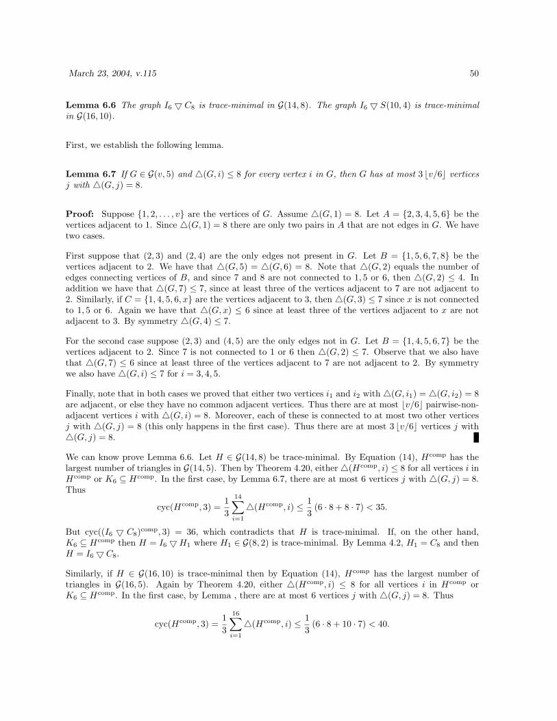
March 23, 2004, v.115 50

Lemma 6.6 The graph I6 5 C8 is trace-minimal in G(14, 8). The graph I6 5 S(10, 4) is trace-minimalin G(16, 10).

First, we establish the following lemma.

Lemma 6.7 If G ∈ G(v, 5) and 4(G, i) ≤ 8 for every vertex i in G, then G has at most 3 bv/6c verticesj with 4(G, j) = 8.

Proof: Suppose {1, 2, . . . , v} are the vertices of G. Assume 4(G, 1) = 8. Let A = {2, 3, 4, 5, 6} be thevertices adjacent to 1. Since 4(G, 1) = 8 there are only two pairs in A that are not edges in G. We havetwo cases.

First suppose that (2, 3) and (2, 4) are the only edges not present in G. Let B = {1, 5, 6, 7, 8} be thevertices adjacent to 2. We have that 4(G, 5) = 4(G, 6) = 8. Note that 4(G, 2) equals the number ofedges connecting vertices of B, and since 7 and 8 are not connected to 1, 5 or 6, then 4(G, 2) ≤ 4. Inaddition we have that 4(G, 7) ≤ 7, since at least three of the vertices adjacent to 7 are not adjacent to2. Similarly, if C = {1, 4, 5, 6, x} are the vertices adjacent to 3, then 4(G, 3) ≤ 7 since x is not connectedto 1, 5 or 6. Again we have that 4(G, x) ≤ 6 since at least three of the vertices adjacent to x are notadjacent to 3. By symmetry 4(G, 4) ≤ 7.

For the second case suppose (2, 3) and (4, 5) are the only edges not in G. Let B = {1, 4, 5, 6, 7} be thevertices adjacent to 2. Since 7 is not connected to 1 or 6 then 4(G, 2) ≤ 7. Observe that we also havethat 4(G, 7) ≤ 6 since at least three of the vertices adjacent to 7 are not adjacent to 2. By symmetrywe also have 4(G, i) ≤ 7 for i = 3, 4, 5.

Finally, note that in both cases we proved that either two vertices i1 and i2 with 4(G, i1) = 4(G, i2) = 8are adjacent, or else they have no common adjacent vertices. Thus there are at most bv/6c pairwise-non-adjacent vertices i with 4(G, i) = 8. Moreover, each of these is connected to at most two other verticesj with 4(G, j) = 8 (this only happens in the first case). Thus there are at most 3 bv/6c vertices j with4(G, j) = 8.

We can know prove Lemma 6.6. Let H ∈ G(14, 8) be trace-minimal. By Equation (14), Hcomp has thelargest number of triangles in G(14, 5). Then by Theorem 4.20, either 4(Hcomp, i) ≤ 8 for all vertices i inHcomp or K6 ⊆ Hcomp. In the first case, by Lemma 6.7, there are at most 6 vertices j with 4(G, j) = 8.Thus

cyc(Hcomp, 3) =13

14∑i=1

4(Hcomp, i) ≤ 13

(6 · 8 + 8 · 7) < 35.

But cyc((I6 5 C8)comp, 3) = 36, which contradicts that H is trace-minimal. If, on the other hand,K6 ⊆ Hcomp then H = I6 5H1 where H1 ∈ G(8, 2) is trace-minimal. By Lemma 4.2, H1 = C8 and thenH = I6 5 C8.

Similarly, if H ∈ G(16, 10) is trace-minimal then by Equation (14), Hcomp has the largest number oftriangles in G(16, 5). Again by Theorem 4.20, either 4(Hcomp, i) ≤ 8 for all vertices i in Hcomp orK6 ⊆ Hcomp. In the first case, by Lemma , there are at most 6 vertices j with 4(G, j) = 8. Thus

cyc(Hcomp, 3) =13

16∑i=1

4(Hcomp, i) ≤ 13

(6 · 8 + 10 · 7) < 40.

March 23, 2004, v.115 51

But cyc((I6 5 S(10, 4))comp, 3) = 40, which contradicts that H is trace-minimal. If, on the other hand,K6 ⊆ Hcomp then H = I65H1 where H1 ∈ G(10, 4) is trace-minimal. By Lemma 6.3, H1 = S(10, 4) andthen H = I6 5 S(10, 4).

7 Proofs of Theorems 2.1 and 2.3

The proofs of Theorems 2.1 and 2.3 depend on an application of the Coefficient Theorem [Sa1], [CDS,Theorem 1.3] to regular graphs [Sa2], [CDS, Theorem 3.26]. We summarize these results now. Let H bea regular graph in G(v, δ) with girth h and let xv + a1x

v−1 + · · · + av be the characteristic polynomialof A(H). Then the coefficient ai for i ≤ 2h − 1 depends only on the numbers of cycles in H, cyc(H, j),with j ≤ i and not on the particular structure of the graph H. Indeed a1 = 0 and a2 = vδ. For i ≥ 3,there exist integers u(q, i) for q = 0, 3 ≤ q ≤ i, and i + q even, such that for every H ∈ G(v, δ) with girthh and i ≤ 2h− 1,

ai = (−1)i2 u(0, i)− 2cyc(H, i)− 2

∑(−1)

i+q2 cyc(H, q)u(q, i), (21)

where u(0, i) = 0 if i is odd, and the sum is taken over integers q satisfying h ≤ q < i and i + q even.

We also require Newton’s Identities [BP] in matrix form. Let X be a v × v matrix with characteristicpolynomial det(xI −X) = xv + c1x

v−1 + c2xv−2 + · · · cn. Then for all q ≤ v,

0 = trXq + c1trXq−1 + c2trXq−2 + · · ·+ qcq.

Proof: Theorem 2.1 Suppose that the graph G ∈ G(v, δ) satisfies the hypotheses of the theorem. LetH be a graph in G(v, δ) with girth h, and let

ch(G, x) = xv + b1xv−1 + · · ·+ bv,

ch(H,x) = xv + a1xv−1 + · · ·+ av.

By the hypothesis, cyc(G, q) = cyc(H, q) for all q < k and cyc(G, k) < cyc(H, k). Since G has themaximum girth in G(v, δ), h ≤ g. There are two cases.

Case I h < g: In this case cyc(H, q) = cyc(G, q) = 0 for all q < h, cyc(G, h) = 0, and cyc(H,h) > 0.(Thus k = h.) Applying Equation (21) to H,G and i < h, we get

ai = bi = (−1)i2 u(0, i).

Thus from Newton’s Identities we have trA(H)i = trA(G)i for i < h.

For i = h, Equation (21) gives

ah = (−1)h2 u(0, h)− 2cyc(H,h),

bh = (−1)h2 u(0, h).

Since cyc(H,h) > 0, ah < bh. By Newton’s Identities trA(G)h < trA(H)h. Thus G is trace-dominatedby H.

Case II h = g: In this case k ≥ g. Let i < k. Then cyc(H, q) = cyc(G, q) for all q < i so the expressionsin Equation (21) for ai and bi are identical. Thus ai = bi and it follows from Newton’s Identities thattrA(H)i = trA(G)i for i < k.

March 23, 2004, v.115 52

The only place where the expressions in Equation (21) for ak and bk differ is −2cyc(H, k) and −2cyc(G, k).Since cyc(G, k) < cyc(H, k), we have ak < bk. Thus from Newton’s Identities we have trA(G)k <trA(H)k. So G is trace-dominated by H.

To prove Theorem 2.3 we need the following Lemma:

Lemma 7.1 Let G, H be graphs in G(v, δ). Suppose G is connected and has k + 1 eigenvalues. IftrA(G)i = trA(H)i for i = 2, . . . , 2k− 1 then either spec(A(G)) = spec(A(H)) or trA(G)2k < trA(H)2k,which implies that G is trace-dominated by H.

Proof: Theorem 2.3 Let G ∈ G(v, δ) satisfy the hypotheses of the theorem. Let H ∈ G(v, δ) havegirth h. We show that G is trace-dominated by H.

If h < g, then the same argument as in Case I of the proof of Theorem 2.1 shows that G is trace-dominatedby H.

Now suppose that h ≥ g. Then for i < g, cyc(H, i) = cyc(G, i) = 0 and hence from Equation (21) andNewton’s Identities we have trA(H)i = trA(G)i. If g is even, then g = 2k and if g is odd then g = 2k +1.Either way i ≤ 2k for all i < g. Thus by Lemma 7.1 G is trace-dominated by H.

All that remains is the proof of Lemma 7.1. We need the following lemma:

Lemma 7.2 Let λ and µ be multi-sets of real numbers with cardinality N . Suppose λ has k distinctvalues λ1, . . . , λk with multiplicities ni > 0 and µ has h distinct values µ1, . . . , µh with multiplicitiesmi > 0. If

∑ki=1 niλ

ji =

∑hi=1 miµ

ji for j = 1, . . . , 2k − 1 then,

∑ki=1 niλ

2ki ≤

∑hi=1 miµ

2ki , with equality

if and only if λ = µ.

Proof:

Define a polynomial q(y) = (y − λ1) · · · (y − λk). Clearly,

q(y)2 = y2k + h1y2k−1 + · · ·+ h2k,

where hi is an integral polynomial in λ1, . . . , λk. Let x = (x1, . . . , xN ), where xi are independent inde-terminates and define a polynomial by

f(x1, . . . , xN ) =N∑

t=1

q(xt)2.

Thenf(x) = S2k(x) + h1S2k−1(x) + · · ·+ Nh2k,

where Sj(x) =∑

xjt is the jth power sum of x. Clearly f(λ) = 0 and since Sj(λ) = Sj(µ) for j =

1, . . . , 2k − 1, we havef(µ) = f(µ)− f(λ) = S2k(µ)− S2k(λ).

But f(µ) ≥ 0 since it is a sum of squares of real numbers. It follows that S2k(λ) ≤ S2k(µ).

Now suppose S2k(λ) = S2k(µ). Then f(µ) = 0 and so the distinct values of µ are among the distinctvalues λ1, . . . , λk of λ. In particular h ≤ k and by interchanging the roles of λ and µ, we get h = k. Sowe may assume that µi = λi for i = 1, . . . , k.

March 23, 2004, v.115 53

We have∑k

i=1(mi − ni)λji = 0 for j = 1, . . . , k. But the van der Monde matrix based on λi is invertible

and so mi = ni, for i = 1, . . . , k. that is, λ = µ.

We now apply Lemma 7.2 to the reduced spectrum of the adjacency matrix of a graph to finish the proofof Lemma 7.1.

Let G ∈ G(v, δ) be connected with adjacency matrix A(G) such that spec(A(G)) has k + 1 distinctvalues. Since G is δ-regular and connected, δ is a simple eigenvalue of A(G). Thus the reduced spectrumspec′(A(G)) = λ of A(G) has k distinct eigenvalues λi with multiplicity ni for i = 1, . . . , k, where∑

i ni = v− 1. Let H be a δ-regular graph with adjacency matrix A(H) with reduced spectrum µ havingh distinct eigenvalues µ1, . . . , µh with multiplicities m1, . . . ,mh. Denote the power-sums of λ and µ by

Sj(λ) = trA(G)j − dj =∑k

i=1 ni λji

Sj(µ) = trA(H)j − dj =∑h

i=1 mi µji .

By the hypothesis of the lemma, Sj(λ) = Sj(µ) for 1 ≤ j ≤ 2k − 1. It follows from Lemma 7.2 thatS2k(λ) ≤ S2k(µ). If S2k(λ) < S2k(µ), we are finished. Otherwise S2k(λ) = S2k(µ) and then it followsfrom Lemma 7.2 that λ = µ, that is A(G) and A(H) have the same spectrum. The proof of Lemma 7.1is complete.

March 23, 2004, v.115 54

References

[AFNW] B. Abrego, S. Fernandez-Merchant, M. G. Neubauer, and W. Watkins, D-optimal weighingdesigns for n ≡ −1 (mod 4) objects and a large number of weighings, Linear Algebra Appl.,374 (2003) 175-218.

[Bri] G. Brinkmann, Fast generation of cubic graphs, J. Graph Theory, 23 (1996) 139-149.

[BP] W.S. Burnside, A.W. Panton, The Theory of Equations with an Introduction to the Theory ofBinary Algebraic Forms, Dover, New York, 1960.

[Co] J.H.E. Cohn, Determinants with elements ±1, J. London Math. Soc., 42 (1967) 436-442.

[CDS] D. Cvetkovic, M. Doob and H. Sachs, Spectra of Graphs, Theory and Application, AcademicPress, New York, 1980.

[CRC] The CRC Handbook of Combinatorial Design, Eds. C.J. Colbourn and J.H. Dinitz, CRC Press,Boca Raton, 1996.

[FG] H.-J. Finck, G. Grohmann, Vollstandiges Produkt, chromatische Zahl und charakteristischesPolynom regularer Graphen, I. Wiss. Z. TH Ilmenau, 11 (1965) 1-3.

[God] C.D. Godsil, Problems in algebraic combinatorics, Electron. J. Combin. F1 (1995).

[Gor] Gordon’s Data. www.cs.uwa.edu.au/˜gordon/data.html

[Ho] H. Hotelling, Some improvements in weighing and other experimental techniques, Ann. Math.Statist., 15 (1944) 297-306.

[HKL] M. Hudelson, V. Klee and D. Larman, Largest j-simplices in d-cubes: Some relatives of theHadamard determinant problem, Linear Algebra Appl., 241 (1996) 519-598.

[Mo] A.M. Mood, On Hotelling’s weighing problem, Ann. Math. Statist., 17 (1946), 432-446.

[NR] M. Neubauer and A.J. Radcliffe, The maximum determinant of (±1)-matrices, Linear AlgebraAppl., 257 (1997) 289-306.

[NWZ1] M. Neubauer, W. Watkins and J. Zeitlin, Notes on D-optimal designs, Linear Algebra Appl.,280 (1998) 109-127.

[NWZ2] M. Neubauer, W. Watkins and J. Zeitlin, Maximal D-optimal weighing designs for 4 and 5objects, Electron. J. Linear Algebra, 4 (1998) 48-72, http://math.technion.ac.il/iic/ela.

[NWZ3] M. Neubauer, W. Watkins and J. Zeitlin, D-optimal weighing designs for six objects, Metrika,52 (2000) 185-211.

[NW] M. Neubauer and W. Watkins, D-optimal designs for seven objects and a large number ofweighings, Linear and Multilinear Algebra, 50 (2002) 61-74.

[Pu] F. Pukelsheim, Optimal Design of Experiments, Wiley, New York, 1993.

[PW] N. Pullman and N. Wormald, Regular graphs with prescribed odd girth, Utilitas Math., 24(1983) 243-251.

[Ri] T. Rivlin, The Chebyshev Polynomials, Wiley, New York, 1974.

[RW] R.W. Robinson and W.C. Wormald, Number of cubic graphs, J. Graph Theory, 7 (1983)463-467.

[Sa1] H. Sachs, Uber die Anzahlen von Baumen, Waldern und Kreisen gegebenen Typs in gegebenenGraphen, Habilitationsschrift Univ. Halle, Math.-Nat. Fak. (1963).

[Sa2] H. Sachs, Beziehungen zwischen den in einem Graphen enthaltenen Kreisen und seinem charak-teristischen Polynom, Publ. Math. Debrecen 11 (1964) 119-134.

[St] F.W. Stevenson, Projective Planes, Freeman, San Francisco, 1972.

[vM] H. van Maldeghem, Generalized Polygons, Monographs in Mathematics Vol. 93, BirkhauserVerlag, Basel, (1998)

[vLW] J.H. van Lint and R.M. Wilson, A Course in Combinatorics, Cambridge University Press,Cambridge, 1992.

[Ya] F. Yates, Complex experiments, J. Roy. Statist. Soc. Supp. 2 (1935) 181-247.

55

Trace-minimal graphs and D-optimal weighing designsba70714/publications/tracemin.pdfTrace-minimal...

Documents

Transcript of Trace-minimal graphs and D-optimal weighing designsba70714/publications/tracemin.pdfTrace-minimal...