Topics in Time Series Econometrics Structural VAR › 2013 › ... · Topics in Time Series...
37
Topics in Time Series Econometrics Structural VAR Domenico Giannone, Université Libre de Bruxelles and CEPR
Transcript of Topics in Time Series Econometrics Structural VAR › 2013 › ... · Topics in Time Series...
Topics in Time Series EconometricsStructural VAR
Domenico Giannone, Université Libre de Bruxelles andCEPR
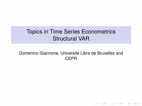
Trend stationary processes
yt = Tt + Ct
Trend (deterministic):Tt = α + δt
Cycle (stationary process):Ct = ψ(L)et = et + ψ1et−1 + ψ2et−2 + ... et ∼WN(0, σ2)
• Shocks have only temporary effects
∂Ct+h
∂et= ψh → 0 as h→∞
yt+h|t − yt+h|t−1 = ψhet
⇒ All deviation from the deterministic trend are temporary
Remark: yt+h|t = δ(t + h) + ψhet + ψh−1et−1 + ψh−2et−2 + ...
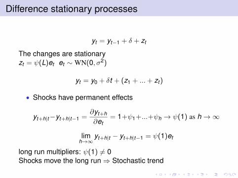
Difference stationary processes
yt = yt−1 + δ + zt
The changes are stationaryzt = ψ(L)et et ∼WN(0, σ2)
yt = y0 + δt + (z1 + ...+ zt )
• Shocks have permanent effects
yt+h|t−yt+h|t−1 =∂yt+h
∂et= 1+ψ1+...+ψh → ψ(1) as h→∞
limh→∞
yt+h|t − yt+h|t−1 = ψ(1)et
long run multipliers: ψ(1) 6= 0Shocks move the long run⇒ Stochastic trend

Stochastic or deterministic trend?
Nelson and Plosser, 1986, Journal of Monetary Economics
The authors cannot reject the hypothesis that most of themacroeconomic time series for the US are non stationarystochastic processes with no tendency to return to adeterministic path.
⇒ Shocks that drive the long run trend might also be drivingbusiness cycle fluctuations (Real Business Cycles)
This findings cast doubts on the importance ofdemand/monetary shocks as the main sources of businesscycles fluctuations
⇒ debate on the relative importance of demand and supplyshocks as driving forces for business cycle fluctuations
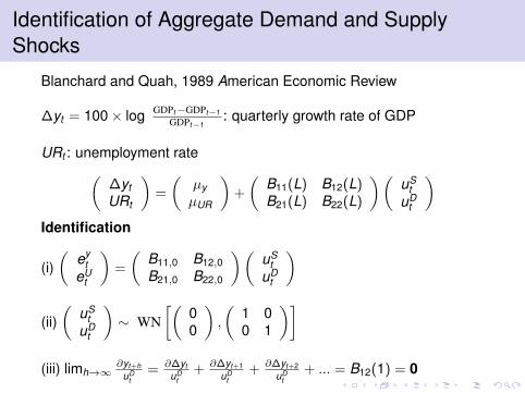
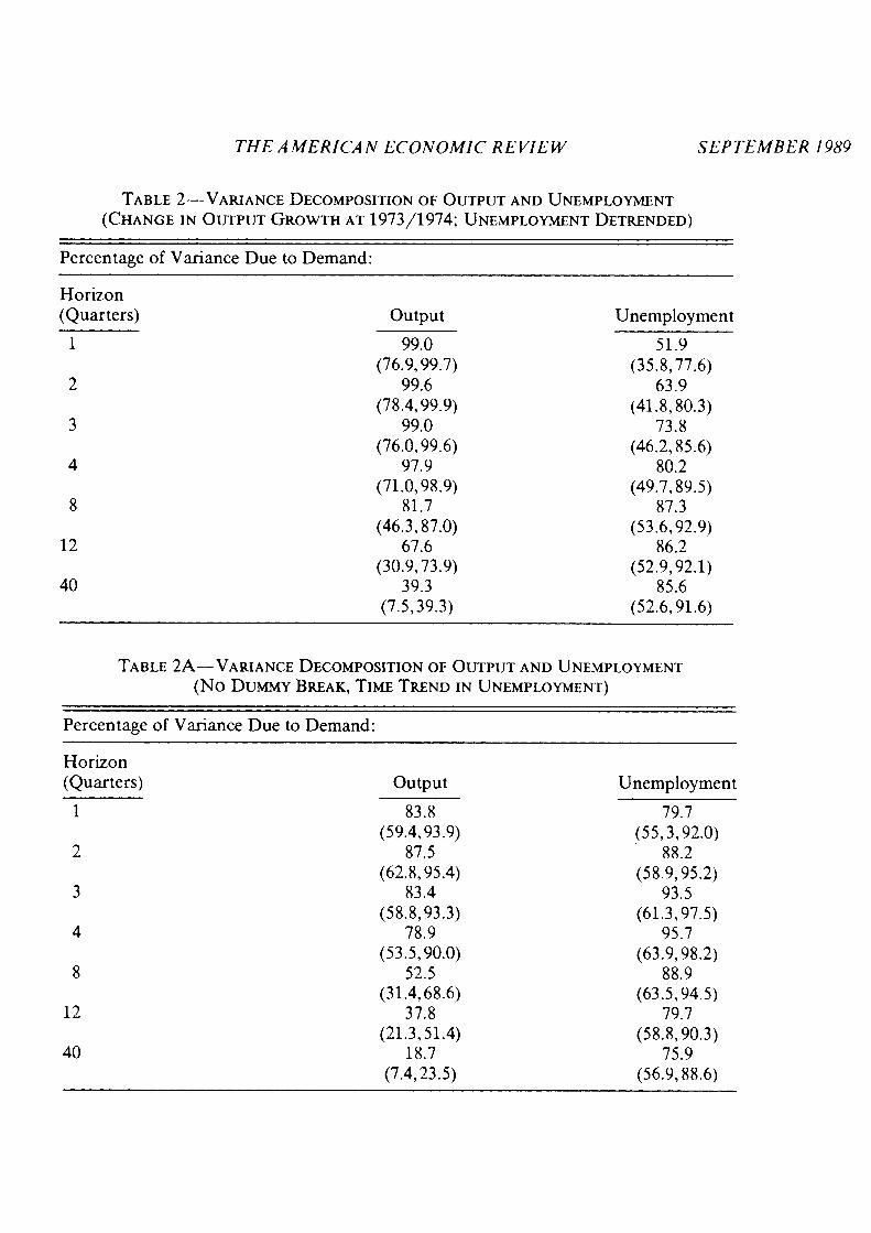
Identification of Aggregate Demand and SupplyShocks
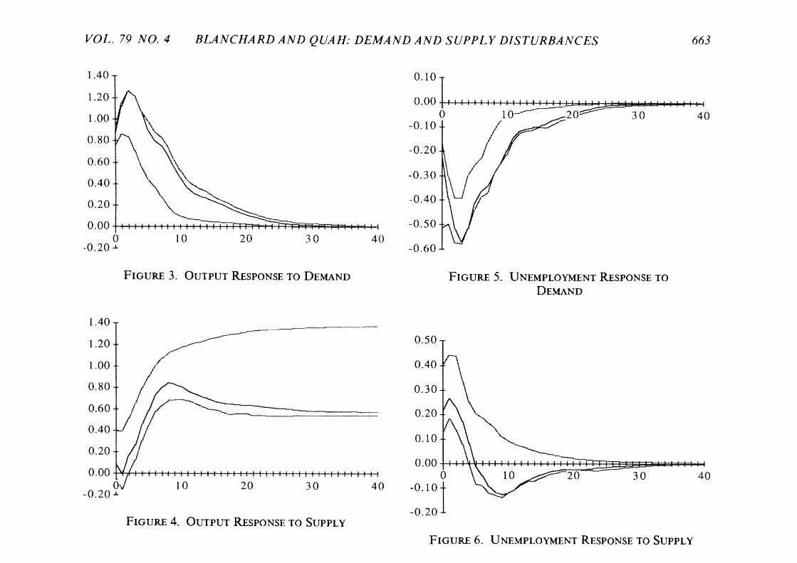
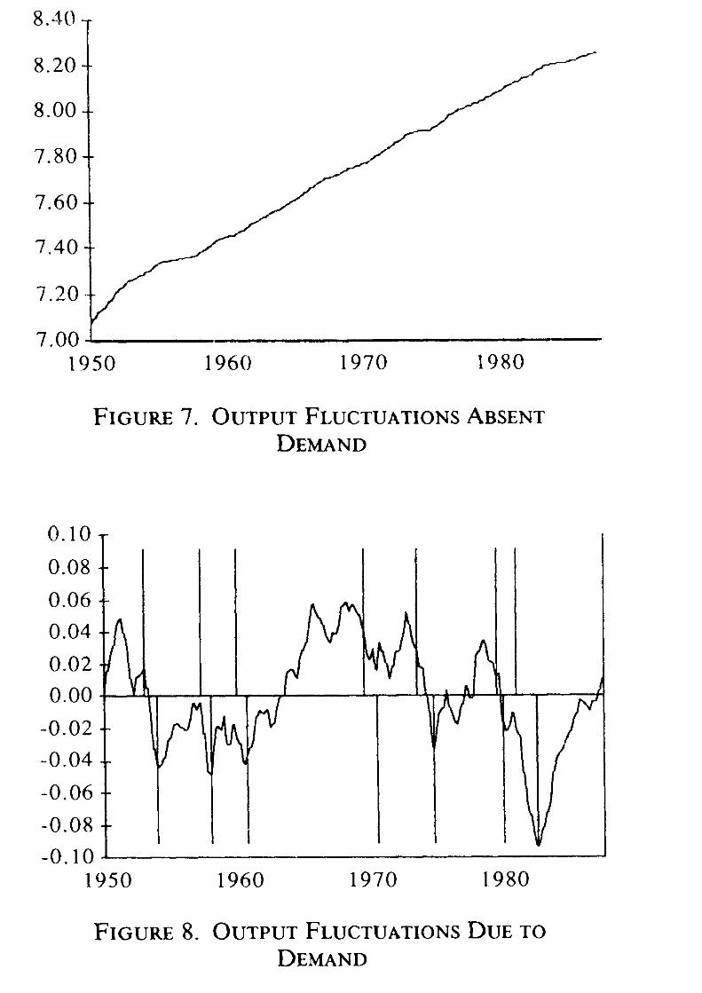
Blanchard and Quah, 1989 American Economic Review
∆yt = 100× log GDPt−GDPt−1GDPt−1
: quarterly growth rate of GDP
URt : unemployment rate(∆ytURt
)=
(µyµUR
)+
(B11(L) B12(L)B21(L) B22(L)
)(uS
tuD
t
)Identification
(i)(
eyt
eUt
)=
(B11,0 B12,0B21,0 B22,0
)(uS
tuD
t
)
(ii)(
uSt
uDt
)∼ WN
[(00
),
(1 00 1
)](iii) limh→∞
∂yt+huD
t= ∂∆yt
uDt
+ ∂∆yt+1uD
t+ ∂∆yt+2
uDt
+ ... = B12(1) = 0
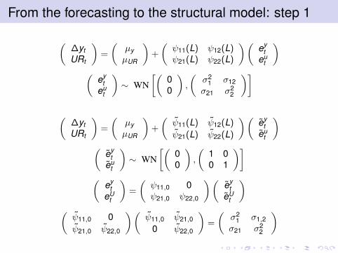
From the forecasting to the structural model: step 1
(∆ytURt
)=
(µyµUR
)+
(ψ11(L) ψ12(L)ψ21(L) ψ22(L)
)(ey
teu
t
)(
eyt
eut
)∼ WN
[(00
),
(σ2
1 σ12σ21 σ2
2
)](
∆ytURt
)=
(µyµUR
)+
(ψ11(L) ψ12(L)
ψ21(L) ψ22(L)
)(ey
teu
t
)(
eyt
eut
)∼ WN
[(00
),
(1 00 1
)](
eyt
eUt
)=
(ψ11,0 0ψ21,0 ψ22,0
)(ey
teU
t
)(ψ11,0 0ψ21,0 ψ22,0
)(ψ11,0 ψ21,0
0 ψ22,0
)=
(σ2
1 σ1,2σ21 σ2
2
)
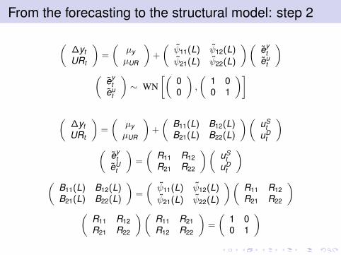
From the forecasting to the structural model: step 2
(∆ytURt
)=
(µyµUR
)+
(ψ11(L) ψ12(L)
ψ21(L) ψ22(L)
)(ey
teu
t
)(
eyt
eut
)∼ WN
[(00
),
(1 00 1
)](
∆ytURt
)=
(µyµUR
)+
(B11(L) B12(L)B21(L) B22(L)
)(uS
tuD
t
)(
eyt
eUt
)=
(R11 R12R21 R22
)(uS
tuD
t
)(
B11(L) B12(L)B21(L) B22(L)
)=
(ψ11(L) ψ12(L)
ψ21(L) ψ22(L)
)(R11 R12R21 R22
)(
R11 R12R21 R22
)(R11 R21R12 R22
)=
(1 00 1
)
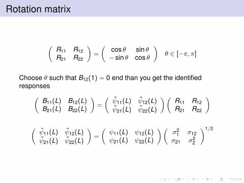
Rotation matrix
(R11 R12R21 R22
)=
(cos θ sin θ− sin θ cos θ
)θ ∈ [−π, π]
Choose θ such that B12(1) = 0 end than you get the identifiedresponses(
B11(L) B12(L)B21(L) B22(L)
)=
(ψ11(L) ψ12(L)
ψ21(L) ψ22(L)
)(R11 R12R21 R22
)(ψ11(L) ψ12(L)
ψ21(L) ψ22(L)
)=
(ψ11(L) ψ12(L)ψ21(L) ψ22(L)
)(σ2
1 σ12σ21 σ2
2
)1/2
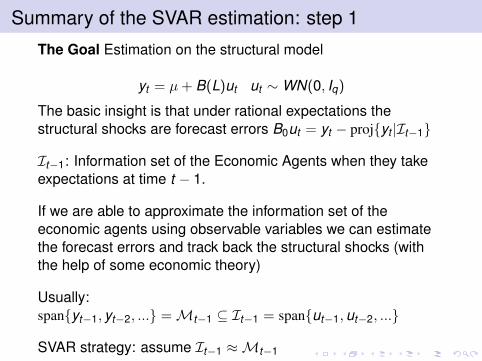
Summary of the SVAR estimation: step 1
The Goal Estimation on the structural model
yt = µ+ B(L)ut ut ∼WN(0, Iq)
The basic insight is that under rational expectations thestructural shocks are forecast errors B0ut = yt − proj{yt |It−1}
It−1: Information set of the Economic Agents when they takeexpectations at time t − 1.
If we are able to approximate the information set of theeconomic agents using observable variables we can estimatethe forecast errors and track back the structural shocks (withthe help of some economic theory)
Usually:span{yt−1, yt−2, ...} =Mt−1 ⊆ It−1 = span{ut−1,ut−2, ...}
SVAR strategy: assume It−1 ≈Mt−1
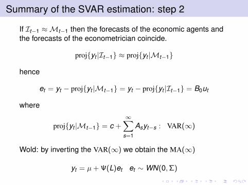
Summary of the SVAR estimation: step 2
If It−1 ≈Mt−1 then the forecasts of the economic agents andthe forecasts of the econometrician coincide.
proj{yt |It−1} ≈ proj{yt |Mt−1}
hence
et = yt − proj{yt |Mt−1} = yt − proj{yt |It−1} = B0ut
where
proj{yt |Mt−1} = c +∞∑
s=1
Asyt−s : VAR(∞)
Wold: by inverting the VAR(∞) we obtain the MA(∞)
yt = µ+ Ψ(L)et et ∼WN(0,Σ)
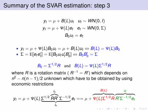
Summary of the SVAR estimation: step 3
yt = µ+ B(L)ut ut ∼WN(0, I)
yt = µ+ Ψ(L)et et ∼WN(0,Σ)
B0ut = et
• yt = µ+ Ψ(L)B0ut = µ+ B(L)ut ⇔ B(L) = Ψ(L)B0• Σ = E[ete′t ] = E[B0utu′tB
′0]⇔ B0B′0 = Σ
B0 = Σ1/2R and B(L) = Ψ(L)Σ1/2R
where R is a rotation matrix ( R−1 = R′) which depends onn2 − n(n − 1)/2 unknown which have to be obtained by usingeconomic restrictions
yt = µ+ Ψ(L) Σ1/2
In︷︸︸︷RR′ Σ−1/2︸ ︷︷ ︸
In
et == µ+
B(L)︷ ︸︸ ︷Ψ(L)Σ1/2R
ut︷ ︸︸ ︷R′Σ−1/2et
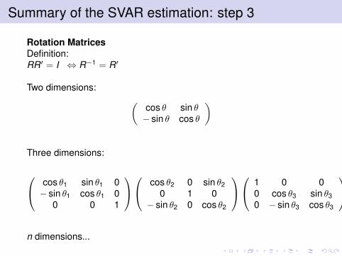
Summary of the SVAR estimation: step 3
Rotation MatricesDefinition:RR′ = I ⇔ R−1 = R′
Two dimensions: (cos θ sin θ− sin θ cos θ
)
Three dimensions:
cos θ1 sin θ1 0− sin θ1 cos θ1 0
0 0 1
cos θ2 0 sin θ20 1 0
− sin θ2 0 cos θ2
1 0 00 cos θ3 sin θ30 − sin θ3 cos θ3
n dimensions...
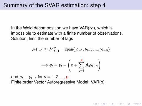
Summary of the SVAR estimation: step 4
In the Wold decomposition we have VAR(∞), which isimpossible to estimate with a finite number of observations.Solution, limit the number of lags
Mt−1 ≈Mpt−1 = span{yt−1, yt−2, ..., yt−p}
=⇒ et = yt −
(c +
p∑s=1
Asyt−s
)and et ⊥ yt−s for s = 1,2, ...,pFinite order Vector Autoregressive Model: VAR(p)
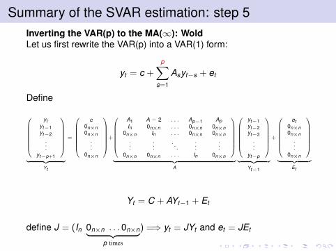
Summary of the SVAR estimation: step 5Inverting the VAR(p) to the MA(∞): WoldLet us first rewrite the VAR(p) into a VAR(1) form:
yt = c +
p∑s=1
Asyt−s + et
Define
ytyt−1yt−2
.
.
.yt−p+1
︸ ︷︷ ︸
Yt
=
c0n×n0n×n
.
.
.0n×n
+
A1 A − 2 . . . Ap−1 ApIn 0n×n . . . 0n×n 0n×n
0n×n In . . . 0n×n 0n×n...
.
.
.. . .
.
.
....
0n×n 0n×n . . . In 0n×n
︸ ︷︷ ︸
A
yt−1yt−2yt−3
.
.
.yt−p
︸ ︷︷ ︸
Yt−1
+
et0n×n0n×n
.
.
.0n×n
︸ ︷︷ ︸
Et
Yt = C + AYt−1 + Et
define J = (In 0n×n . . . 0n×n︸ ︷︷ ︸p times
) =⇒ yt = JYt and et = JEt

Summary of the SVAR estimation: step 5Inverting the VAR(p) to the MA(∞): Wold
Yt = C + AYt−1 + Et
solve it backward
Yt = (Inp − A)−1C +∞∑j=1
AjEt =⇒ yt = J
( ∞∑s=0
Aj
)C +
∞∑j=1
JAjJ ′et
Equating term by term with the wold decomposition
Ψj = JAjJ ′
Ψ(1) = J(Inp − A)−1J ′
µ = J
( ∞∑s=0
Aj
)C = J(Inp − A)−1C = Ψ(1)c
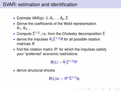
SVAR: estimation and identification
• Estimate VAR(p): c, A1, ..., Ap, Σ
• Derive the coefficients of the Wold representationΨ1, Ψ2, ...
• Compute Σ1/2, i.e. from the Cholesky decomposition Σ
• derive the impulses ΨjΣ1/2R for all possible rotation
matrices R• find the rotation matrix R∗ for which the impulses satisfy
your “preferred” economic restrictions:
B(L) = ΨjΣ1/2R∗
• derive structural shocks
B(L)ut = R∗′Σ1/2et
Widely used identification schemes
• on the contemporaneous multipliers B0: e.g. monetarypolicy shocks, fiscal shocks
• on the lung run multipliers B(1)supply/demand, technology, investment specific shocks
• on the signs at different horizons B0,B1, ,B2, ...supply/demand, monetary policy shocks
• on the shape at different horizons B0,B1, ,B2, ...technological diffusions
• ...
Partial identification
Up to now we have considered have considered the problem ofidentifying all the n shocks⇒ n2 − n(n − 1)/2 restrictions are needed
We are sometimes interested in identifying only a subset ofshocks.
In this case less restrictions are needed since the remainingare left uninterpreted.
If we want to identify only one out of n shock only n − 1restrictions are needed; e.g. only the monetary policy shock inthe system with πt ,URt , rt
If we want to identify two out of n shock only n − 1(n − 2)restrictions are needed
...

Partial identification in recursive schemeSuppose you assume B0 is lower triangular and you want to identifythe j th shock
The restriction is that:
• the variables above the j th line react to the shock only with a lag:slow variables
• the variables below the j th line can react to the shockimmediately: fast variables ...but they affect the j th variables only with a lag
Example: Monetary policy shock:- j th variable is the policy instrument- slow variables (above): prices, real ...- fast variables (above): financial...
The impulse response functions to the j the variables depends only onthe fast/slow grouping... but not on the order within the two groupsSee Christiano, Eichembaum and Evans, 1999.
25ECB
Working Paper Series No 966November 2008
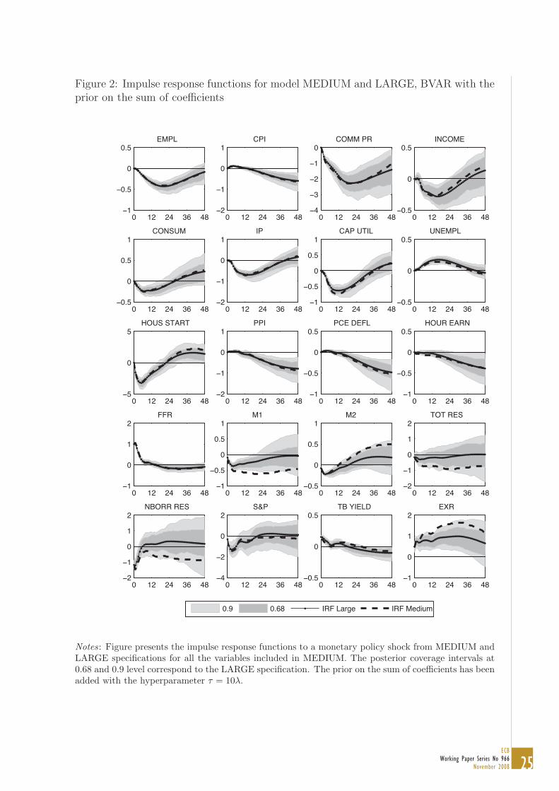
Figure 2: Impulse response functions for model MEDIUM and LARGE, BVAR with theprior on the sum of coefficients
0 12 24 36 48−1
−0.5
0
0.5EMPL
0 12 24 36 48−2
−1
0
1CPI
0 12 24 36 48−4
−3
−2
−1
0COMM PR
0 12 24 36 48−0.5
0
0.5INCOME
0 12 24 36 48−0.5
0
0.5
1CONSUM
0 12 24 36 48−2
−1
0
1IP
0 12 24 36 48−1
−0.5
0
0.5
1CAP UTIL
0 12 24 36 48−0.5
0
0.5UNEMPL
0 12 24 36 48−5
0
5HOUS START
0 12 24 36 48−2
−1
0
1PPI
0 12 24 36 48−1
−0.5
0
0.5PCE DEFL
0 12 24 36 48−1
−0.5
0
0.5HOUR EARN
0 12 24 36 48−1
0
1
2FFR
0 12 24 36 48−1
−0.5
0
0.5
1M1
0 12 24 36 48−0.5
0
0.5
1M2
0 12 24 36 48−2
−1
0
1
2TOT RES
0 12 24 36 48−2
−1
0
1
2NBORR RES
0 12 24 36 48−4
−2
0
2S&P
0 12 24 36 48−0.5
0
0.5TB YIELD
0 12 24 36 48−1
0
1
2EXR
0.9 0.68 IRF Large IRF Medium
Notes: Figure presents the impulse response functions to a monetary policy shock from MEDIUM andLARGE specifications for all the variables included in MEDIUM. The posterior coverage intervals at0.68 and 0.9 level correspond to the LARGE specification. The prior on the sum of coefficients has beenadded with the hyperparameter τ = 10λ.
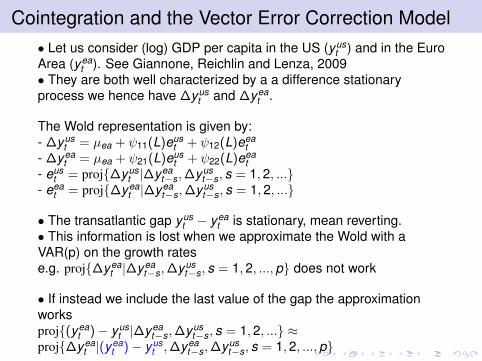
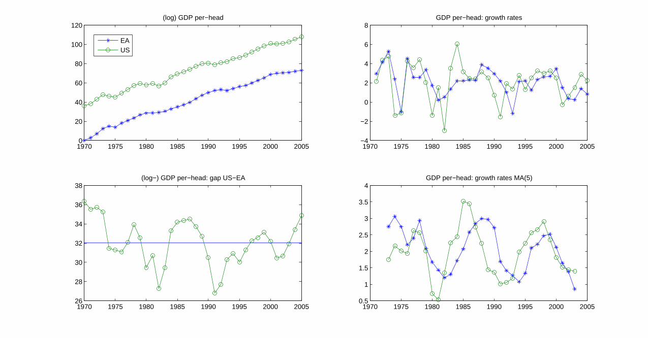
Cointegration and the Vector Error Correction Model• Let us consider (log) GDP per capita in the US (yus
t ) and in the EuroArea (yea
t ). See Giannone, Reichlin and Lenza, 2009• They are both well characterized by a a difference stationaryprocess we hence have ∆yus
t and ∆yeat .
The Wold representation is given by:- ∆yus
t = µea + ψ11(L)eust + ψ12(L)eea
t- ∆yea
t = µea + ψ21(L)eust + ψ22(L)eea
t- eus
t = proj{∆yust |∆yea
t−s,∆yust−s, s = 1,2, ...}
- eeat = proj{∆yea
t |∆yeat−s,∆yus
t−s, s = 1,2, ...}
• The transatlantic gap yust − yea
t is stationary, mean reverting.• This information is lost when we approximate the Wold with aVAR(p) on the growth ratese.g. proj{∆yea
t |∆yeat−s,∆yus
t−s, s = 1,2, ...,p} does not work
• If instead we include the last value of the gap the approximationworksproj{(yea
t )− yust |∆yea
t−s,∆yust−s, s = 1,2, ...} ≈
proj{∆yeat |(yea
t )− yust ,∆yea
t−s,∆yust−s, s = 1,2, ...,p}
1970 1975 1980 1985 1990 1995 2000 20050
20
40
60
80
100
120(log) GDP per−head
1970 1975 1980 1985 1990 1995 2000 200526
28
30
32
34
36
38(log−) GDP per−head: gap US−EA
1970 1975 1980 1985 1990 1995 2000 2005−4
−2
0
2
4
6
8GDP per−head: growth rates
1970 1975 1980 1985 1990 1995 2000 20050.5
1
1.5
2
2.5
3
3.5
4GDP per−head: growth rates MA(5)
EAUS
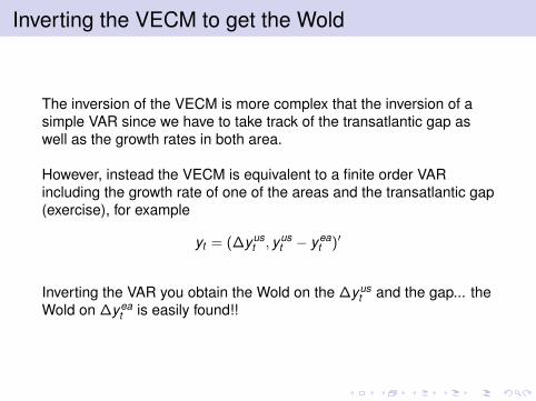
Inverting the VECM to get the Wold
The inversion of the VECM is more complex that the inversion of asimple VAR since we have to take track of the transatlantic gap aswell as the growth rates in both area.
However, instead the VECM is equivalent to a finite order VARincluding the growth rate of one of the areas and the transatlantic gap(exercise), for example
yt = (∆yust , yus
t − yeat )′
Inverting the VAR you obtain the Wold on the ∆yust and the gap... the
Wold on ∆yeat is easily found!!
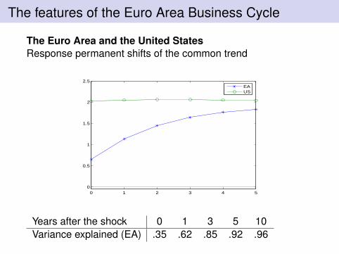
The features of the Euro Area Business Cycle
The Euro Area and the United StatesResponse permanent shifts of the common trend
0 1 2 3 4 50
0.5
1
1.5
2
2.5EAUS
Years after the shock 0 1 3 5 10Variance explained (EA) .35 .62 .85 .92 .96
VAR approximation with cointegrated variables
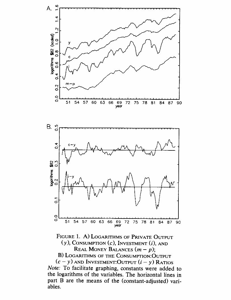
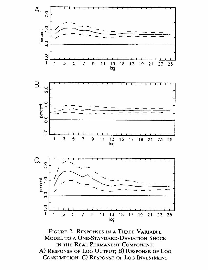
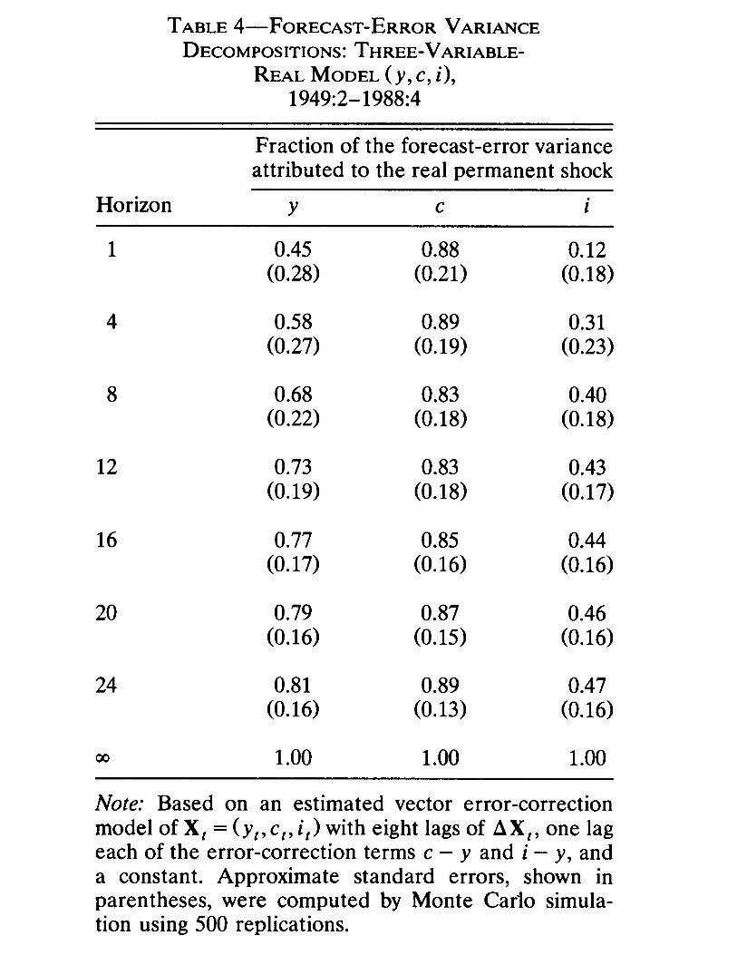
King, Plosser, stock and Watson, 1993Interested in GDP yt , consumption ct and investment it .- ct − yt : consumption ratio is mean reverting- it − yt : investment ratio is mean revertingThey estimate a VAR on
∆yt , ct − yt , it − yt
They identify the productivity shock as the only shock havinglong run effects on yt .Remark Notice that because of the cointegrating relations thetechnology shock will be the only one affecting ct and it(Exercise)

http://www.jstor.org/stable/2006644
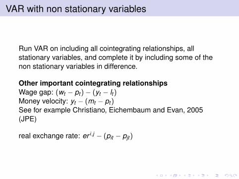
VAR with non stationary variables
Run VAR on including all cointegrating relationships, allstationary variables, and complete it by including some of thenon stationary variables in difference.
Other important cointegrating relationshipsWage gap: (wt − pt )− (yt − lt )Money velocity: yt − (mt − pt )See for example Christiano, Eichembaum and Evan, 2005(JPE)
real exchange rate: er i,j − (pit − pjt )
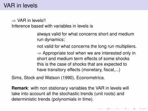
VAR in levels
⇒ VAR in levels!!Inference based with variables in levels is
always valid for what concerns short and mediumrun dynamics;not valid for what concerns the long run multipliers.⇒ Appropriate tool when we are interested only inshort and medium term effects of some shocksthis is the case of shocks that are expected tohave transitory effects (monetary, fiscal,...)
Sims, Stock and Watson (1990), Econometrica.
Remark: with non stationary variables the VAR in levels willtake into account all the stochastic trends (unit roots) anddeterministic trends (polynomials in time).
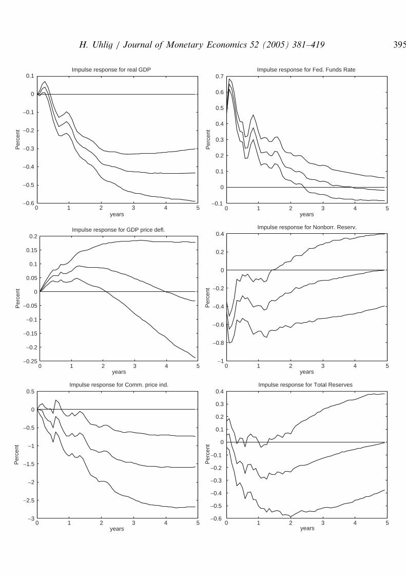
0 1 2 3 4 5−0.6
−0.5
−0.4
−0.3
−0.2
−0.1
0
0.1Impulse response for real GDP
years
Per
cent
0 1 2 3 4 5−0.1
0
0.1
0.2
0.3
0.4
0.5
0.6
0.7Impulse response for Fed. Funds Rate
yearsP
erce
nt
0 1 2 3 4 5−0.25
−0.2
−0.15
−0.1
−0.05
0
0.05
0.1
0.15
0.2Impulse response for GDP price defl.
years
Per
cent
0 1 2 3 4 5−1
−0.8
−0.6
−0.4
−0.2
0
0.2
0.4Impulse response for Nonborr. Reserv.
years
Per
cent
0 1 2 3 4 5−3
−2.5
−2
−1.5
−1
−0.5
0
0.5Impulse response for Comm. price ind.
years
Per
cent
0 1 2 3 4 5−0.6
−0.5
−0.4
−0.3
−0.2
−0.1
0
0.1
0.2
0.3
0.4Impulse response for Total Reserves
years
Per
cent
H. Uhlig / Journal of Monetary Economics 52 (2005) 381–419 395
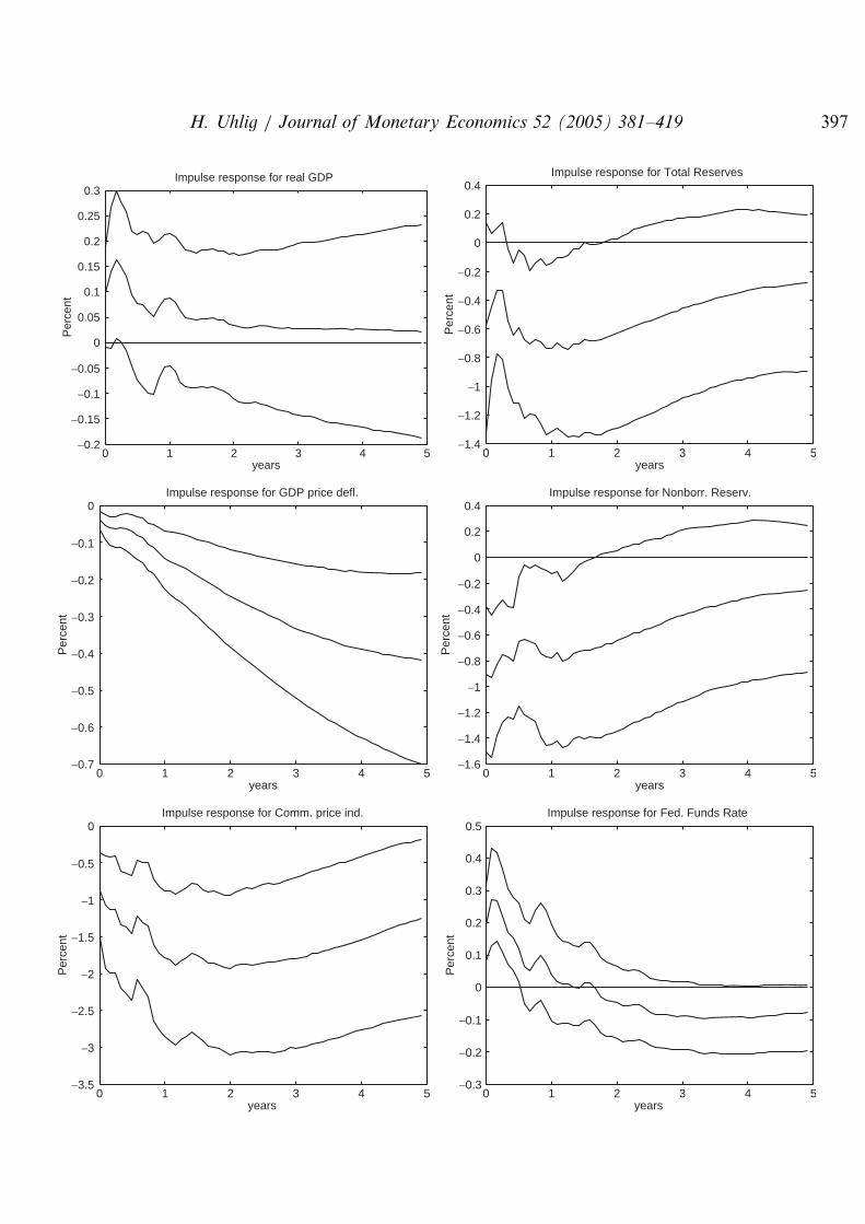
0 1 2 3 4 5−0.2
−0.15
−0.1
−0.05
0
0.05
0.1
0.15
0.2
0.25
0.3Impulse response for real GDP
years
Per
cent
0 1 2 3 4 5−1.4
−1.2
−1
−0.8
−0.6
−0.4
−0.2
0
0.2
0.4Impulse response for Total Reserves
yearsP
erce
nt
0 1 2 3 4 5−0.7
−0.6
−0.5
−0.4
−0.3
−0.2
−0.1
0Impulse response for GDP price defl.
years
Per
cent
0 1 2 3 4 5−1.6
−1.4
−1.2
−1
−0.8
−0.6
−0.4
−0.2
0
0.2
0.4Impulse response for Nonborr. Reserv.
years
Per
cent
0 1 2 3 4 5−3.5
−3
−2.5
−2
−1.5
−1
−0.5
0Impulse response for Comm. price ind.
years
Per
cent
0 1 2 3 4 5−0.3
−0.2
−0.1
0
0.1
0.2
0.3
0.4
0.5Impulse response for Fed. Funds Rate
years
Per
cent
H. Uhlig / Journal of Monetary Economics 52 (2005) 381–419 397