Tom Luo Lecture 4: Linear and quadratic problems
34
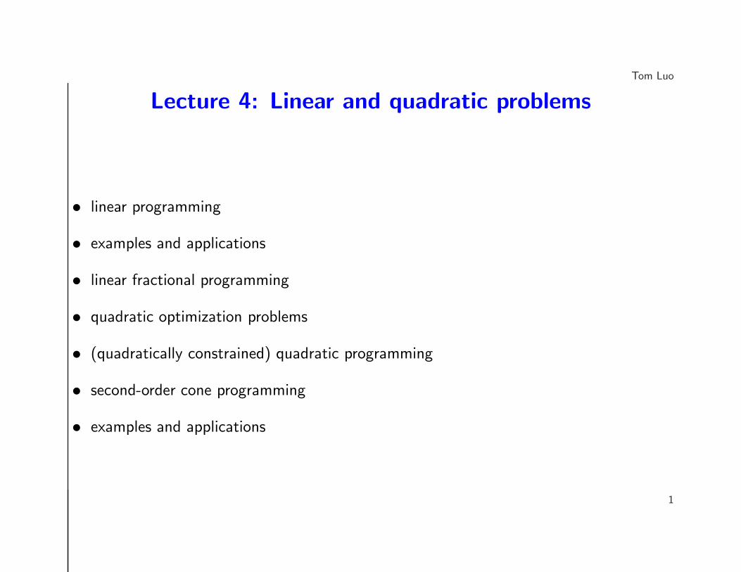
Tom Luo Lecture 4: Linear and quadratic problems • linear programming • examples and applications • linear fractional programming • quadratic optimization problems • (quadratically constrained) quadratic programming • second-order cone programming • examples and applications 1
Transcript of Tom Luo Lecture 4: Linear and quadratic problems
Tom Luo
Lecture 4: Linear and quadratic problems
• linear programming
• examples and applications
• linear fractional programming
• quadratic optimization problems
• (quadratically constrained) quadratic programming
• second-order cone programming
• examples and applications
1
Tom Luo
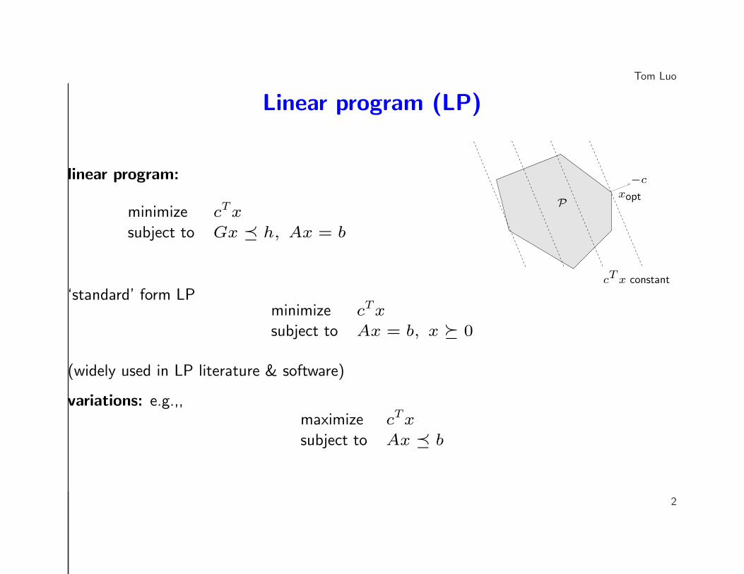
Linear program (LP)
linear program:
minimize cTx
subject to Gx � h, Ax = b
Pxopt
−c
cT x constant
‘standard’ form LPminimize cTx
subject to Ax = b, x � 0
(widely used in LP literature & software)
variations: e.g.,,maximize cTx
subject to Ax � b
2
Tom Luo
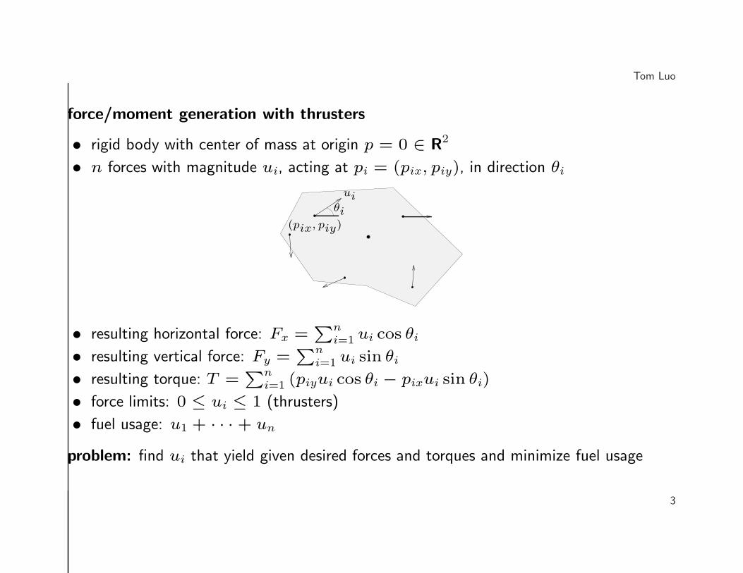
force/moment generation with thrusters
• rigid body with center of mass at origin p = 0 ∈ R2
• n forces with magnitude ui, acting at pi = (pix, piy), in direction θi
ui
(pix, piy)
θi
• resulting horizontal force: Fx =∑n
i=1 ui cos θi• resulting vertical force: Fy =
∑ni=1 ui sin θi
• resulting torque: T =∑n
i=1 (piyui cos θi − pixui sin θi)
• force limits: 0 ≤ ui ≤ 1 (thrusters)
• fuel usage: u1 + · · · + un
problem: find ui that yield given desired forces and torques and minimize fuel usage
3
Tom Luo
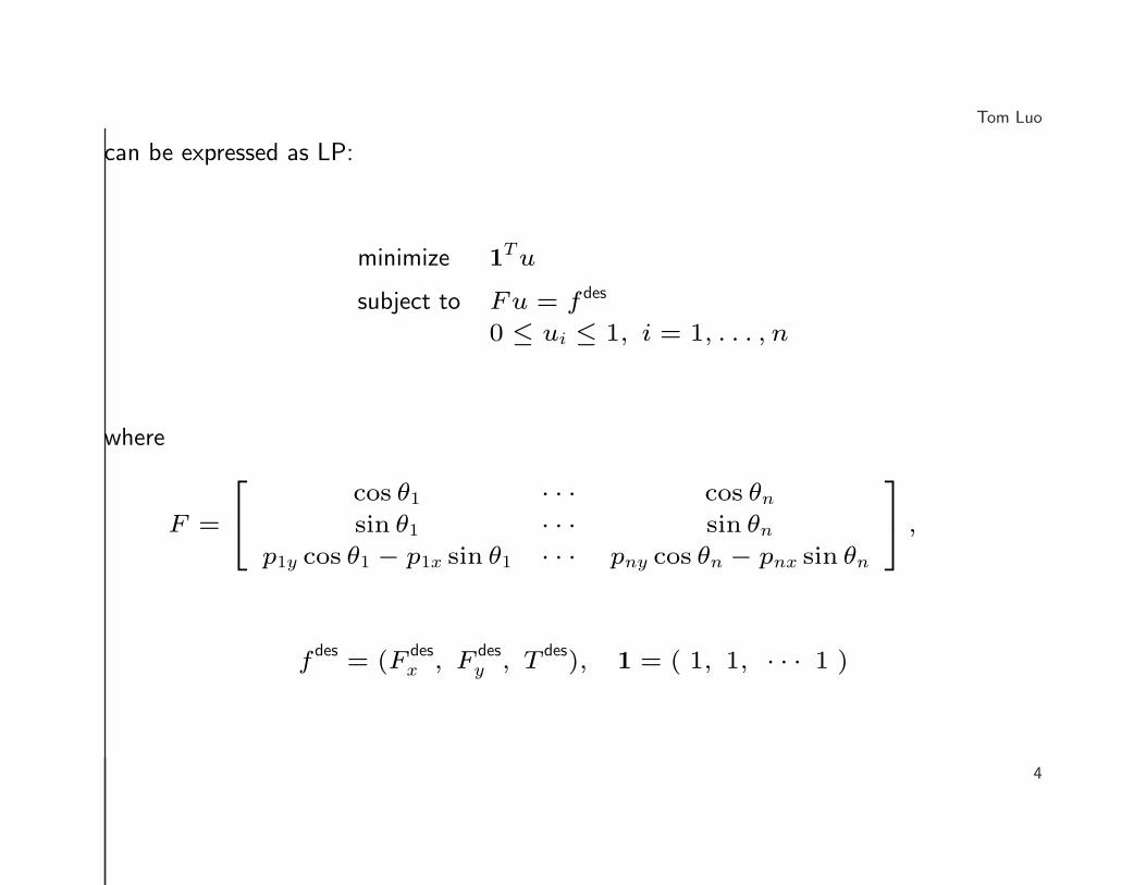
can be expressed as LP:
minimize 1Tu
subject to Fu = f des
0 ≤ ui ≤ 1, i = 1, . . . , n
where
F =
cos θ1 · · · cos θnsin θ1 · · · sin θn
p1y cos θ1 − p1x sin θ1 · · · pny cos θn − pnx sin θn
,
fdes
= (Fdesx , F
desy , T
des), 1 = ( 1, 1, · · · 1 )
4
Tom Luo
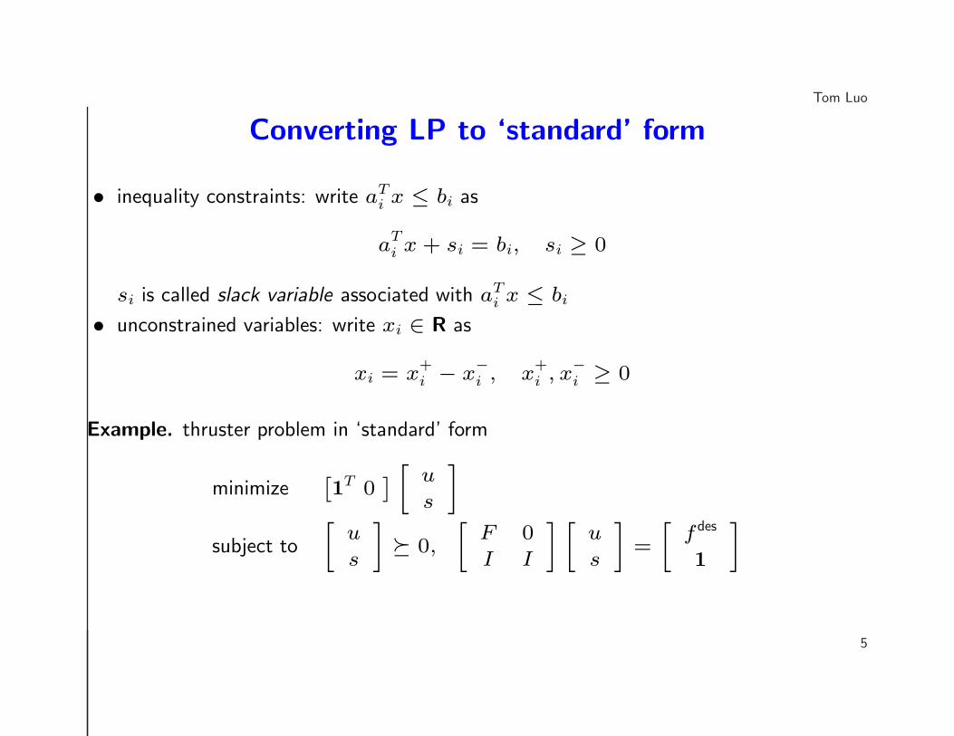
Converting LP to ‘standard’ form
• inequality constraints: write aTi x ≤ bi as
aTi x + si = bi, si ≥ 0
si is called slack variable associated with aTi x ≤ bi
• unconstrained variables: write xi ∈ R as
xi = x+i − x
−i , x
+i , x
−i ≥ 0
Example. thruster problem in ‘standard’ form
minimize[
1T 0
]
[
u
s
]
subject to
[
u
s
]
� 0,
[
F 0
I I
] [
u
s
]
=
[
f des
1
]
5
Tom Luo
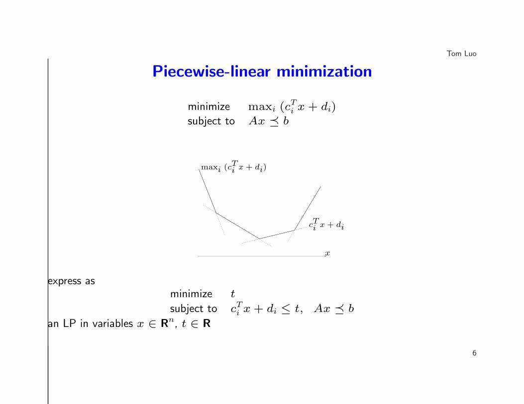
Piecewise-linear minimization
minimize maxi (cTi x + di)
subject to Ax � b
x
cTi x + di
maxi (cTi x + di)
express asminimize t
subject to cTi x + di ≤ t, Ax � b
an LP in variables x ∈ Rn, t ∈ R
6
Tom Luo
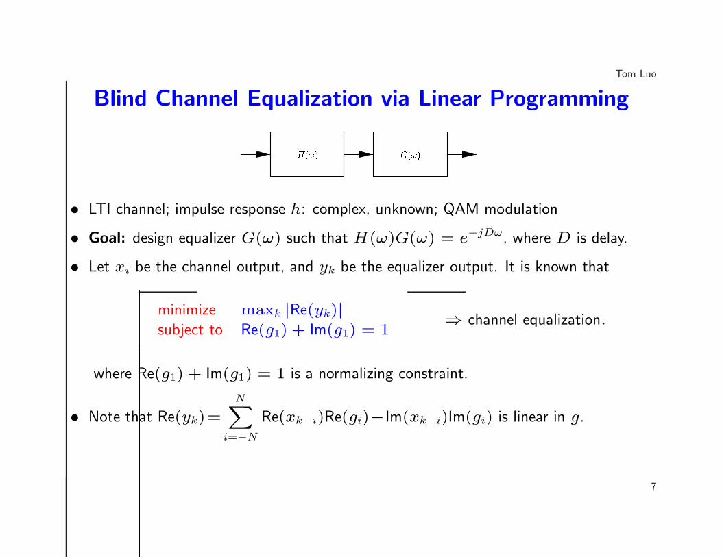
Blind Channel Equalization via Linear Programming
Filter design 13 { 10Equalizer design
PSfrag replacements G(!)H(!)
equalization: given� G (unequalized frequency response)� Gdes (desired frequency response)design (FIR equalizer) H so that gG �= GH � Gdes
� common choice: Gdes(!) = e�jD! (delay)i.e., equalization is deconvolution (up to delay)� can add constraints on H, e.g., limits on jhij ormax! jH(!)j• LTI channel; impulse response h: complex, unknown; QAM modulation
• Goal: design equalizer G(ω) such that H(ω)G(ω) = e−jDω, where D is delay.
• Let xi be the channel output, and yk be the equalizer output. It is known that
minimize maxk |Re(yk)|subject to Re(g1) + Im(g1) = 1
⇒ channel equalization.
where Re(g1) + Im(g1) = 1 is a normalizing constraint.
• Note that Re(yk)=
N∑
i=−N
Re(xk−i)Re(gi)−Im(xk−i)Im(gi) is linear in g.
7
Tom Luo
Blind Channel Equalization via Linear Programming
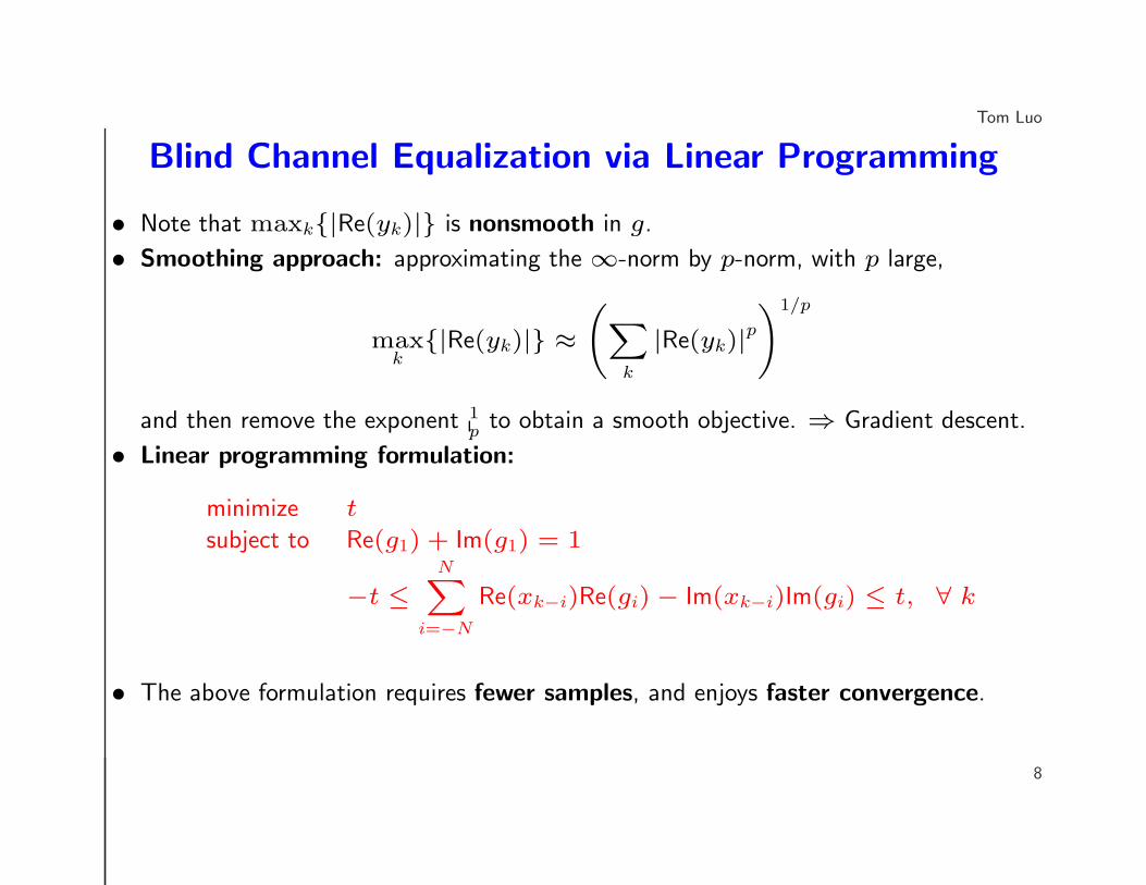
• Note that maxk{|Re(yk)|} is nonsmooth in g.
• Smoothing approach: approximating the ∞-norm by p-norm, with p large,
maxk
{|Re(yk)|} ≈(
∑
k
|Re(yk)|p)1/p
and then remove the exponent 1p to obtain a smooth objective. ⇒ Gradient descent.
• Linear programming formulation:
minimize t
subject to Re(g1) + Im(g1) = 1
−t ≤N∑
i=−N
Re(xk−i)Re(gi) − Im(xk−i)Im(gi) ≤ t, ∀ k
• The above formulation requires fewer samples, and enjoys faster convergence.
8
Tom Luo
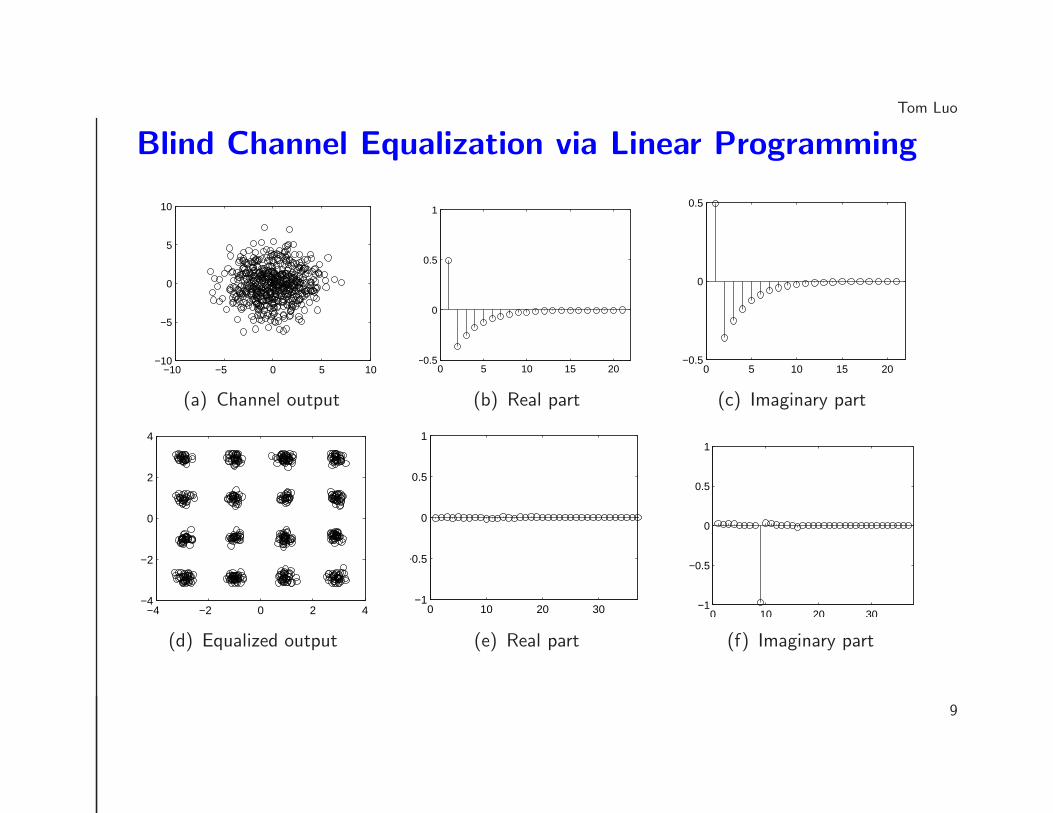
Blind Channel Equalization via Linear Programming
−10 −5 0 5 10−10
−5
0
5
10
(a)
(a) Channel output
0 5 10 15 20−0.5
0
0.5
1
(b)
(b) Real part
0 5 10 15 20−0.5
0
0.5
(c)
(c) Imaginary part
−4 −2 0 2 4−4
−2
0
2
4
(a)
(d) Equalized output
0 10 20 30−1
−0.5
0
0.5
1
(b)
(e) Real part
0 10 20 30−1
−0.5
0
0.5
1
(f) Imaginary part
9
Tom Luo
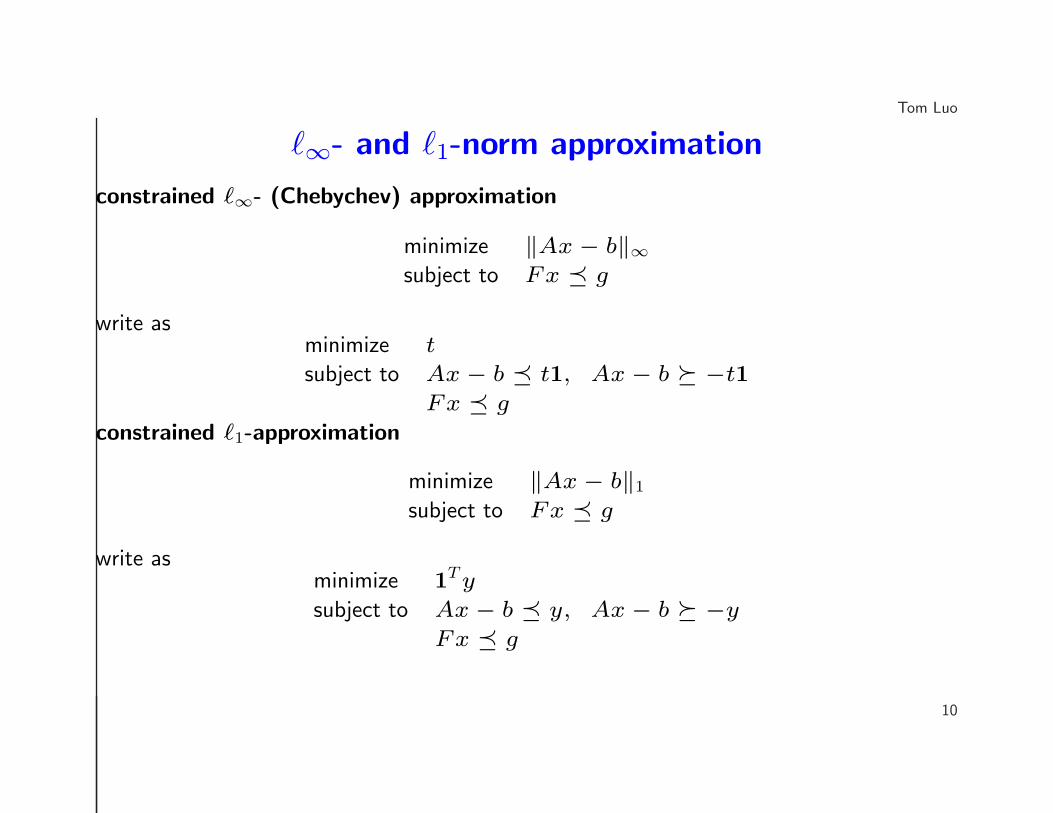
`∞- and `1-norm approximation
constrained `∞- (Chebychev) approximation
minimize ‖Ax − b‖∞subject to Fx � g
write asminimize t
subject to Ax − b � t1, Ax − b � −t1
Fx � g
constrained `1-approximation
minimize ‖Ax − b‖1
subject to Fx � g
write asminimize 1
Ty
subject to Ax − b � y, Ax − b � −y
Fx � g
10
Tom Luo
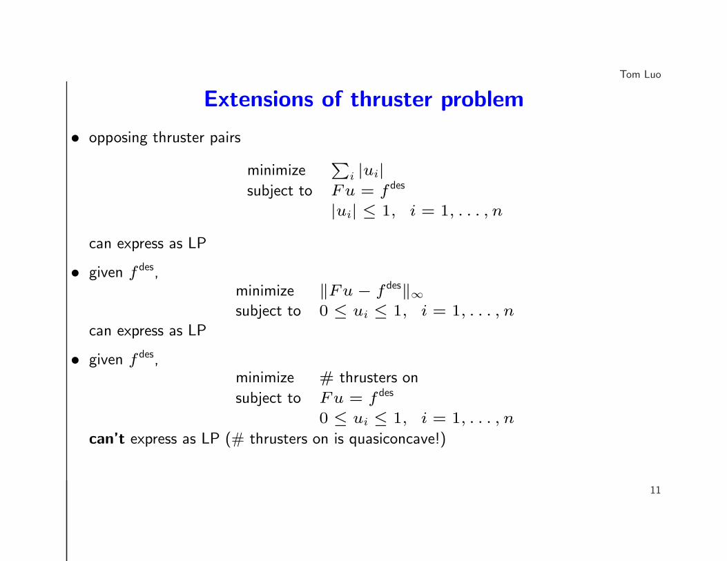
Extensions of thruster problem
• opposing thruster pairs
minimize∑
i |ui|subject to Fu = f des
|ui| ≤ 1, i = 1, . . . , n
can express as LP
• given f des,minimize ‖Fu − f des‖∞subject to 0 ≤ ui ≤ 1, i = 1, . . . , n
can express as LP
• given f des,minimize # thrusters on
subject to Fu = f des
0 ≤ ui ≤ 1, i = 1, . . . , n
can’t express as LP (# thrusters on is quasiconcave!)
11
Tom Luo
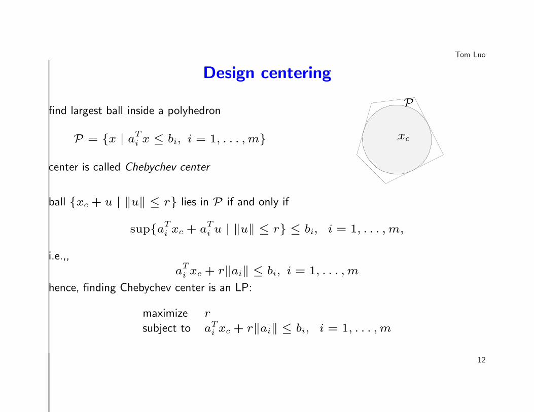
Design centering
find largest ball inside a polyhedron
P = {x | aTi x ≤ bi, i = 1, . . . ,m}
center is called Chebychev center
pxc
P
ball {xc + u | ‖u‖ ≤ r} lies in P if and only if
sup{aTi xc + a
Ti u | ‖u‖ ≤ r} ≤ bi, i = 1, . . . ,m,
i.e.,,
aTi xc + r‖ai‖ ≤ bi, i = 1, . . . ,m
hence, finding Chebychev center is an LP:
maximize r
subject to aTi xc + r‖ai‖ ≤ bi, i = 1, . . . ,m
12
Tom Luo
Linear fractional program
minimizecTx + d
fTx + g
subject to Ax � b, fTx + g > 0
• objective function is quasiconvex
• sublevel sets are polyhedra
• like LP, can be solved very efficiently
extension:
minimize maxi=1,...,K
cTi x + di
fTi x + gi
subject to Ax � b, fTi x + gi > 0, i = 1, . . . ,K
• objective function is quasiconvex
• sublevel sets are polyhedra
13
Tom Luo
Minimum-time optimal controlstate space model:
x(t + 1) = Ax(t) + Bu(t), t = 0, 1, . . . ,K
x(0) = x0, ‖u(t)‖∞ ≤ 1, t = 0, 1, . . . ,K
variables: u(0), . . . , u(K)
settling time f(u(0), . . . , u(K)) is
inf {T | x(t) = 0 for T ≤ t ≤ K + 1}f is quasiconvex function of (u(0), . . . , u(K)):
f(u(0), u(1), . . . , u(K)) ≤ T
if and only if for all t = T, . . . , K + 1
x(t) = Atx0 + A
t−1Bu(0) + · · · + Bu(t − 1) = 0
min-time optimal control problem:
minimize f(u(0), u(1), . . . , u(K))
subject to ‖u(t)‖∞ ≤ 1, t = 0, . . . ,K
14
Tom Luo
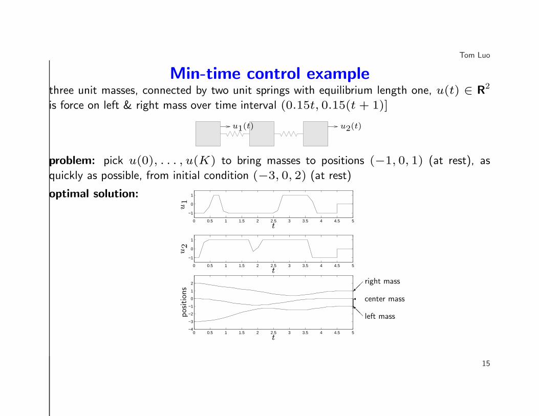
Min-time control examplethree unit masses, connected by two unit springs with equilibrium length one, u(t) ∈ R2
is force on left & right mass over time interval (0.15t, 0.15(t + 1)]
u1(t) u2(t)
problem: pick u(0), . . . , u(K) to bring masses to positions (−1, 0, 1) (at rest), as
quickly as possible, from initial condition (−3, 0, 2) (at rest)
optimal solution:
0 0.5 1 1.5 2 2.5 3 3.5 4 4.5 5
−1
0
1
0 0.5 1 1.5 2 2.5 3 3.5 4 4.5 5
−1
0
1
0 0.5 1 1.5 2 2.5 3 3.5 4 4.5 5−4
−3
−2
−1
0
1
2
t
t
t
u1
u2
positions ��
right mass
@@I left mass
� center mass
15
Tom Luo
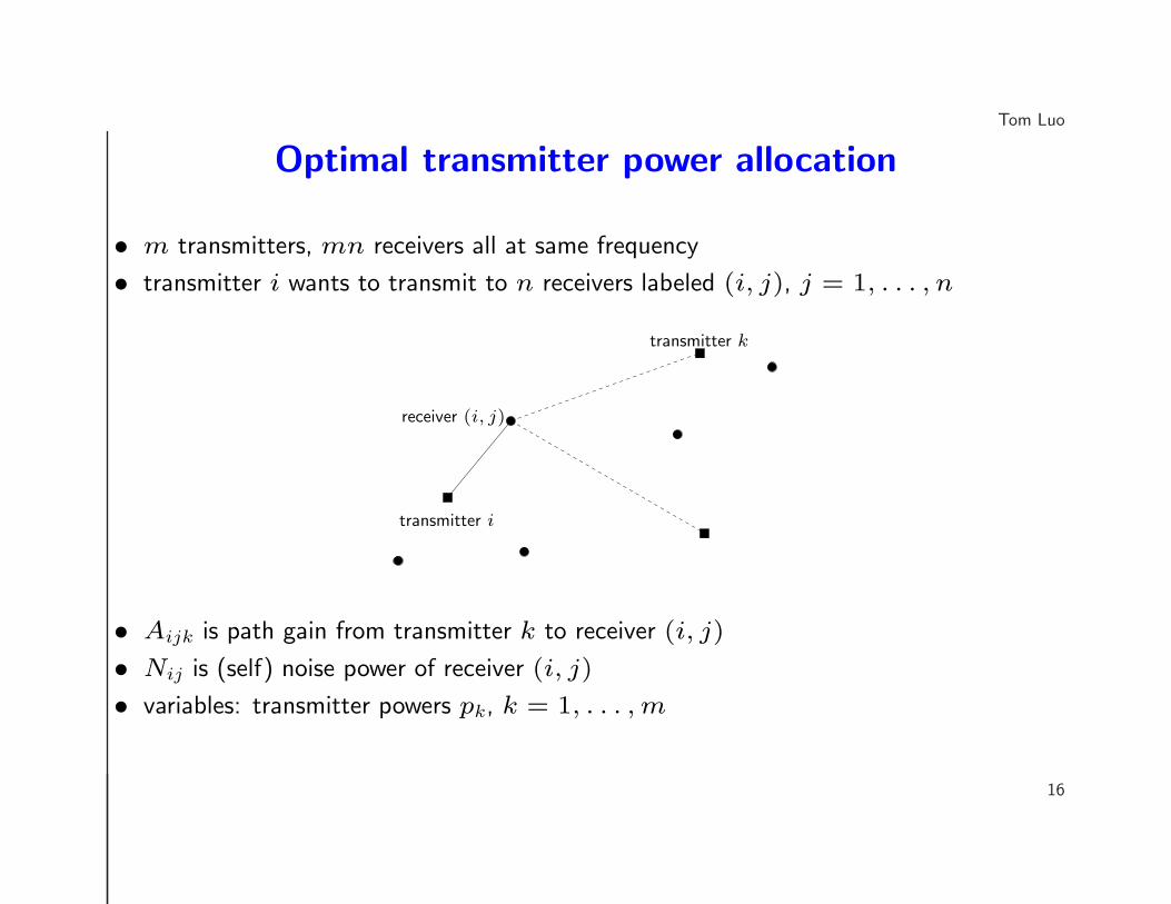
Optimal transmitter power allocation
• m transmitters, mn receivers all at same frequency
• transmitter i wants to transmit to n receivers labeled (i, j), j = 1, . . . , n
transmitter i
transmitter k
receiver (i, j)
• Aijk is path gain from transmitter k to receiver (i, j)
• Nij is (self) noise power of receiver (i, j)
• variables: transmitter powers pk, k = 1, . . . ,m
16
Tom Luo
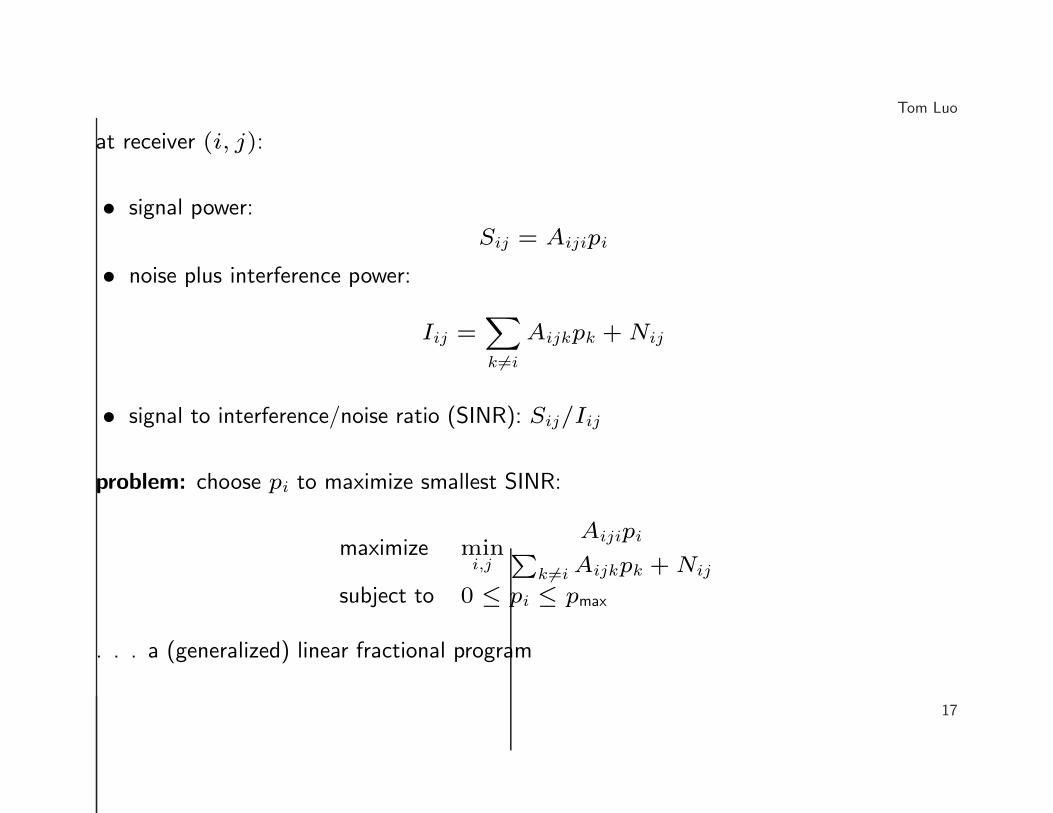
at receiver (i, j):
• signal power:
Sij = Aijipi
• noise plus interference power:
Iij =∑
k 6=i
Aijkpk + Nij
• signal to interference/noise ratio (SINR): Sij/Iij
problem: choose pi to maximize smallest SINR:
maximize mini,j
Aijipi∑
k 6=i Aijkpk + Nij
subject to 0 ≤ pi ≤ pmax
. . . a (generalized) linear fractional program
17
Tom Luo
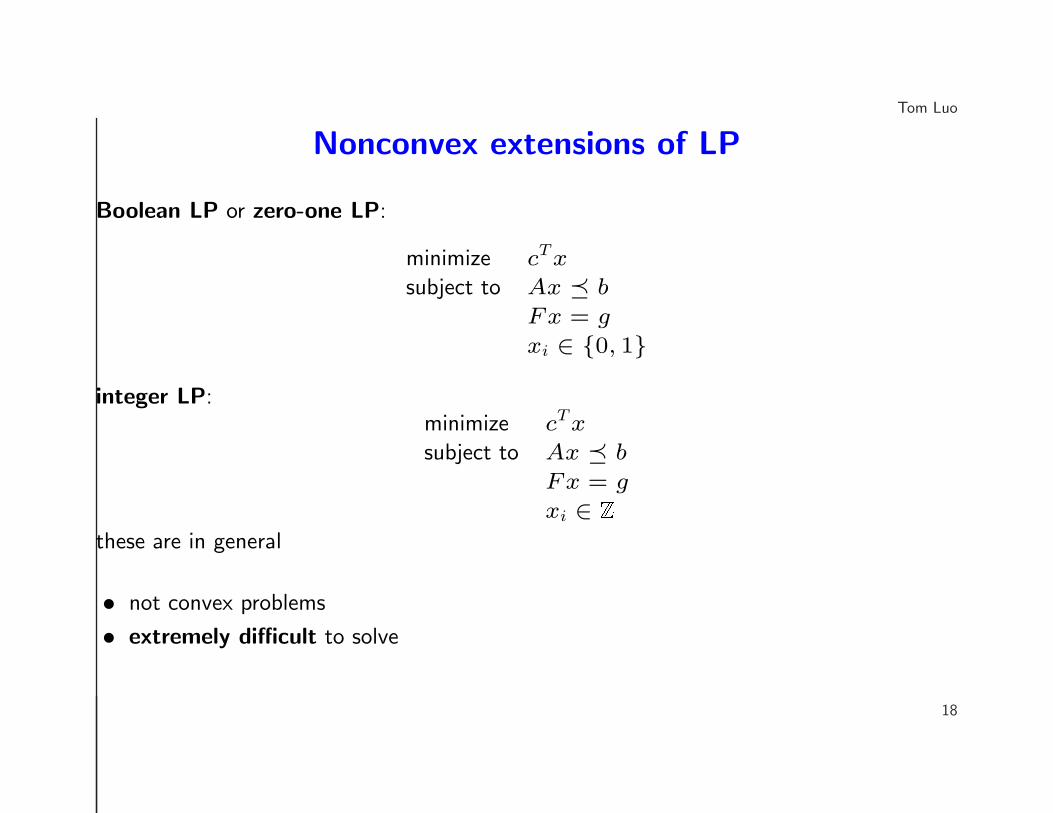
Nonconvex extensions of LP
Boolean LP or zero-one LP:
minimize cTx
subject to Ax � b
Fx = g
xi ∈ {0, 1}
integer LP:minimize cTx
subject to Ax � b
Fx = g
xi ∈ Zthese are in general
• not convex problems
• extremely difficult to solve
18
Tom Luo
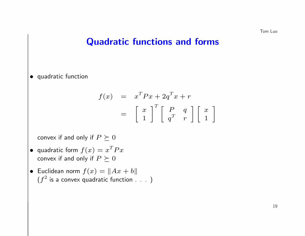
Quadratic functions and forms
• quadratic function
f(x) = xTPx + 2qTx + r
=
[
x
1
]T [P q
qT r
] [
x
1
]
convex if and only if P � 0
• quadratic form f(x) = xTPx
convex if and only if P � 0
• Euclidean norm f(x) = ‖Ax + b‖(f2 is a convex quadratic function . . . )
19
Tom Luo
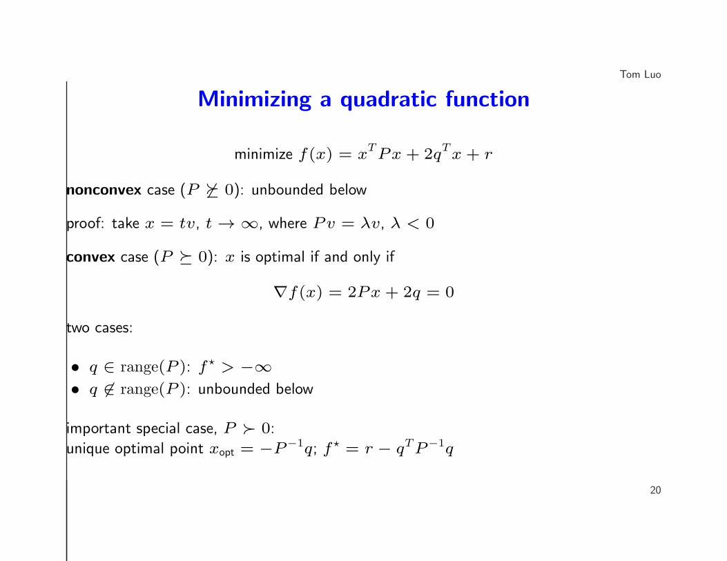
Minimizing a quadratic function
minimize f(x) = xTPx + 2qTx + r
nonconvex case (P 6� 0): unbounded below
proof: take x = tv, t → ∞, where Pv = λv, λ < 0
convex case (P � 0): x is optimal if and only if
∇f(x) = 2Px + 2q = 0
two cases:
• q ∈ range(P ): f? > −∞• q 6∈ range(P ): unbounded below
important special case, P � 0:
unique optimal point xopt = −P−1q; f? = r − qTP−1q
20
Tom Luo
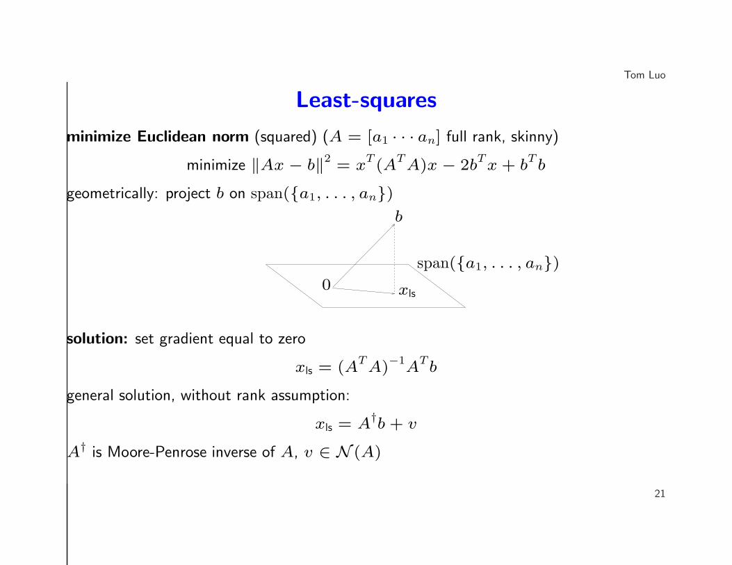
Least-squares
minimize Euclidean norm (squared) (A = [a1 · · · an] full rank, skinny)
minimize ‖Ax − b‖2= x
T(A
TA)x − 2b
Tx + b
Tb
geometrically: project b on span({a1, . . . , an})
span({a1, . . . , an})
b
0 xls
solution: set gradient equal to zero
xls = (ATA)
−1A
Tb
general solution, without rank assumption:
xls = A†b + v
A† is Moore-Penrose inverse of A, v ∈ N (A)
21
Tom Luo
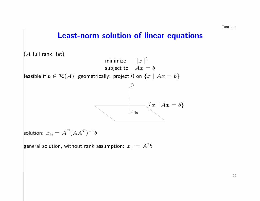
Least-norm solution of linear equations
(A full rank, fat)minimize ‖x‖2
subject to Ax = b
feasible if b ∈ R(A) geometrically: project 0 on {x | Ax = b}
{x | Ax = b}
0
xln
solution: xln = AT(AAT )−1b
general solution, without rank assumption: xln = A†b
22
Tom Luo
Extension: linearly constrained least-squares
minimize ‖Ax − b‖subject to Cx = d
(C ∈ Rr×s full rank, skinny)
can be solved by elimination: write
{x | Cx = d} = {Fw + g | w ∈ Rs−r}
• span(F ) = nullspace(C)
• Cg = d (any solution)
and solve
minimize ‖AFw + Ag − b‖(may or may not be a good idea in practice)
23
Tom Luo
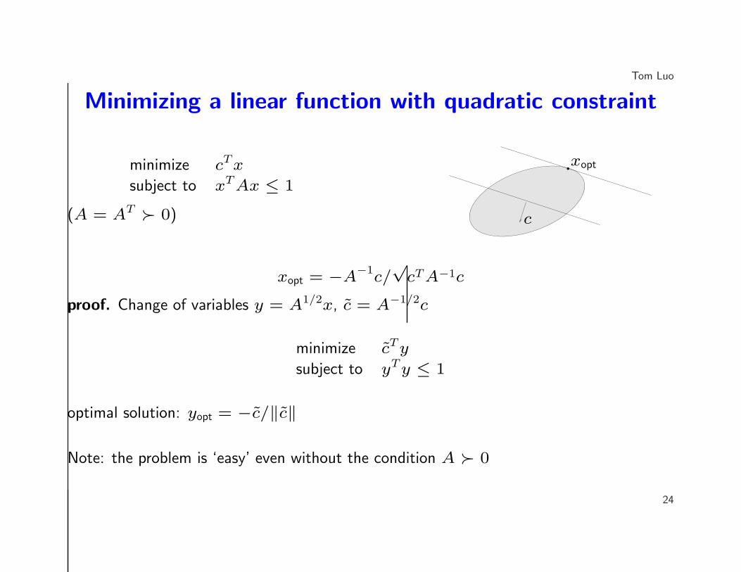
Minimizing a linear function with quadratic constraint
minimize cTx
subject to xTAx ≤ 1
(A = AT � 0) c
xopt
xopt = −A−1
c/√cTA−1c
proof. Change of variables y = A1/2x, c = A−1/2c
minimize cTy
subject to yTy ≤ 1
optimal solution: yopt = −c/‖c‖
Note: the problem is ‘easy’ even without the condition A � 0
24
Tom Luo
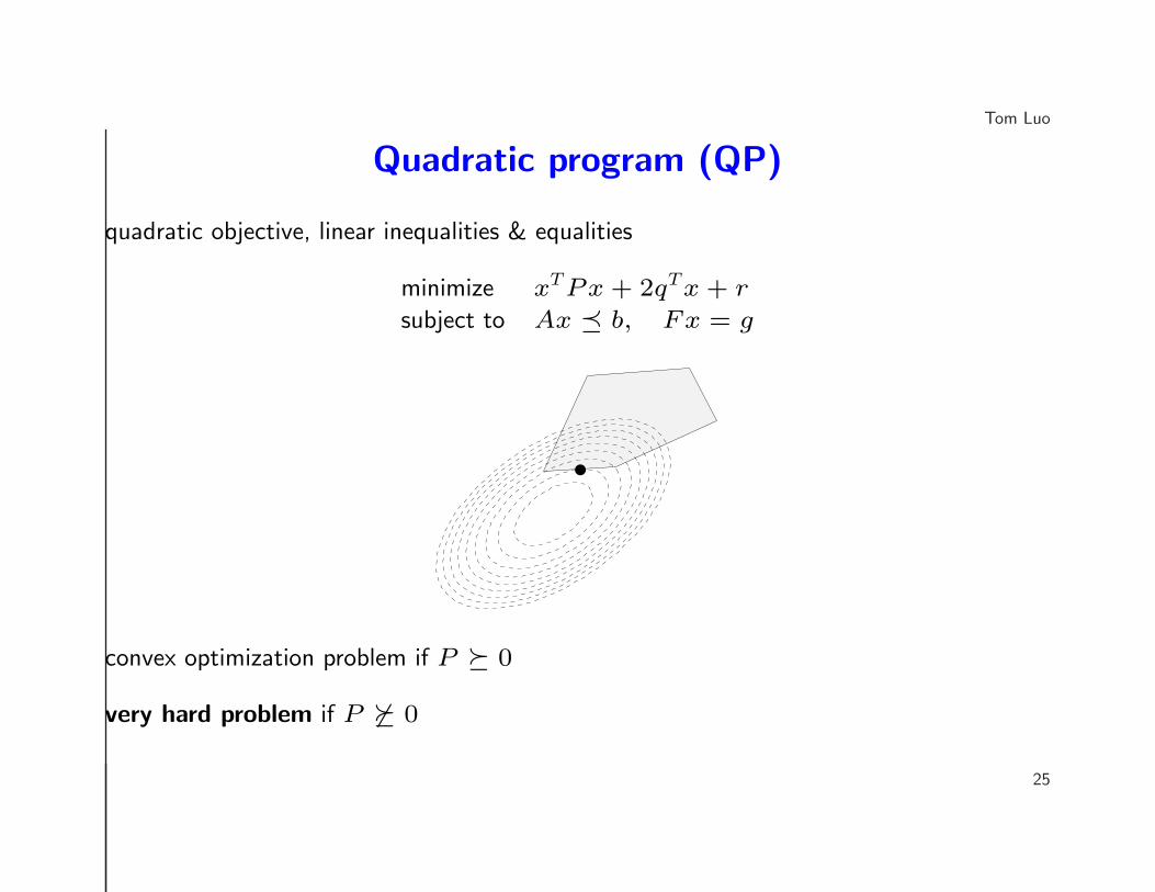
Quadratic program (QP)
quadratic objective, linear inequalities & equalities
minimize xTPx + 2qTx + r
subject to Ax � b, Fx = g
•
convex optimization problem if P � 0
very hard problem if P 6� 0
25
Tom Luo
QCQP and SOCP
quadratically constrained quadratic programming (QCQP):
minimize xTP0x + 2qT0 x + r0
subject to xTPix + 2qTi x + ri ≤ 0, i = 1, . . . , L
• convex if Pi � 0, i = 0, . . . , L
• nonconvex QCQP very difficult
second-order cone programming (SOCP):
minimize cTx
subject to ‖Aix + bi‖ ≤ eTi x + di, i = 1, . . . , L
includes QCQP (QP, LP)
26
Tom Luo
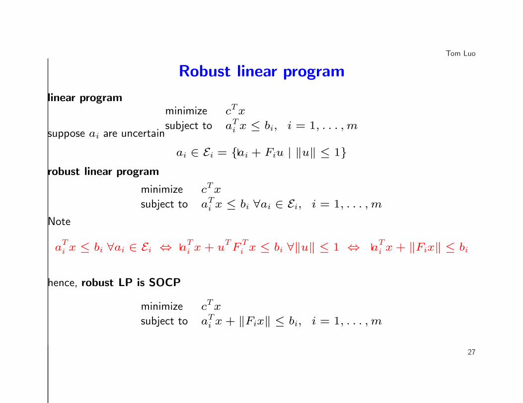
Robust linear program
linear programminimize cTx
subject to aTi x ≤ bi, i = 1, . . . ,m
suppose ai are uncertain
ai ∈ Ei = {ai + Fiu | ‖u‖ ≤ 1}robust linear program
minimize cTx
subject to aTi x ≤ bi ∀ai ∈ Ei, i = 1, . . . ,m
Note
aTi x ≤ bi ∀ai ∈ Ei ⇔ a
Ti x + u
TF
Ti x ≤ bi ∀‖u‖ ≤ 1 ⇔ a
Ti x + ‖Fix‖ ≤ bi
hence, robust LP is SOCP
minimize cTx
subject to aTi x + ‖Fix‖ ≤ bi, i = 1, . . . ,m
27
Tom Luo
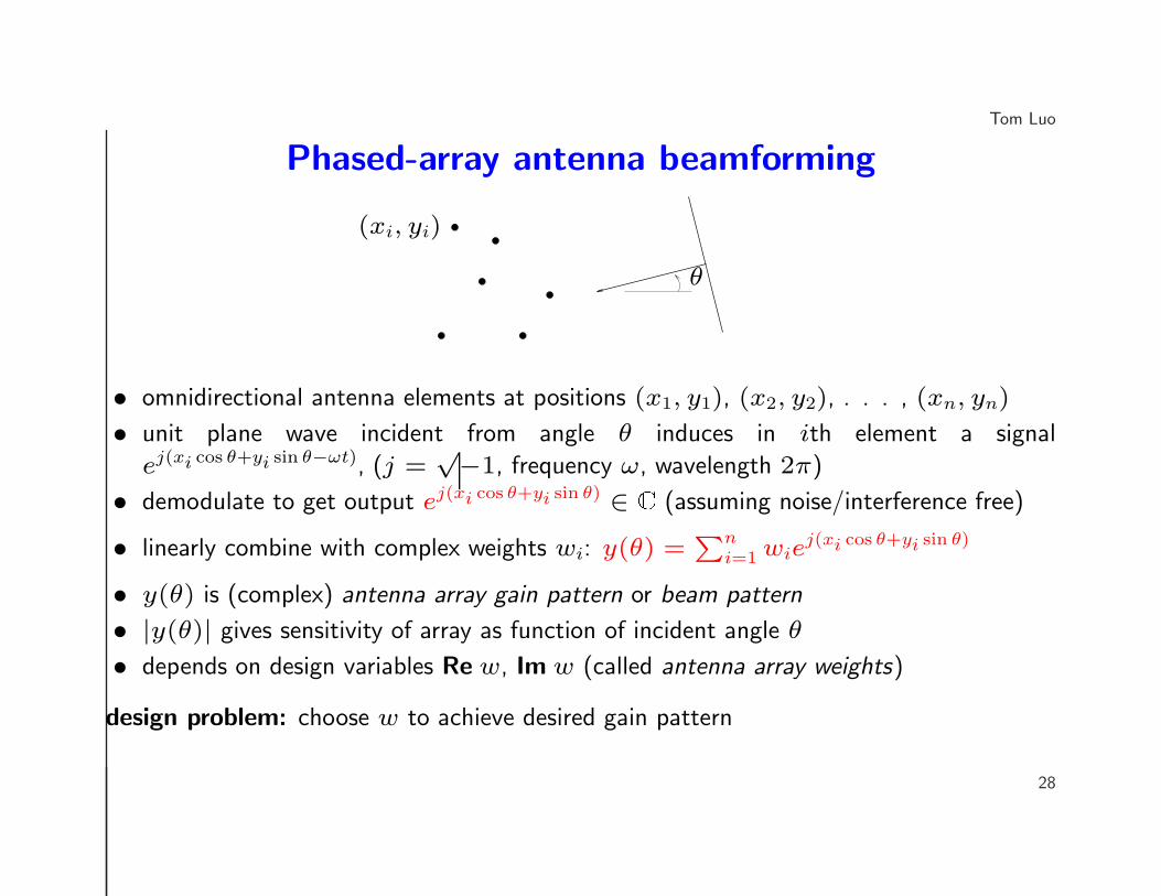
Phased-array antenna beamforming
(xi, yi)
θ
• omnidirectional antenna elements at positions (x1, y1), (x2, y2), . . . , (xn, yn)
• unit plane wave incident from angle θ induces in ith element a signal
ej(xi cos θ+yi sin θ−ωt), (j =√−1, frequency ω, wavelength 2π)
• demodulate to get output ej(xi cos θ+yi sin θ) ∈ C (assuming noise/interference free)
• linearly combine with complex weights wi: y(θ) =∑n
i=1 wiej(xi cos θ+yi sin θ)
• y(θ) is (complex) antenna array gain pattern or beam pattern
• |y(θ)| gives sensitivity of array as function of incident angle θ
• depends on design variables Re w, Im w (called antenna array weights)
design problem: choose w to achieve desired gain pattern
28
Tom Luo
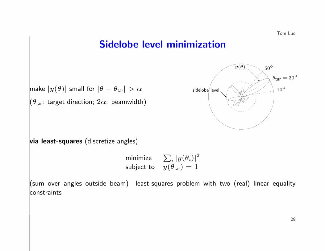
Sidelobe level minimization
make |y(θ)| small for |θ − θtar| > α
(θtar: target direction; 2α: beamwidth)
θtar = 30◦50◦
10◦
@@@R
|y(θ)|
@@Rsidelobe level
via least-squares (discretize angles)
minimize∑
i |y(θi)|2subject to y(θtar) = 1
(sum over angles outside beam) least-squares problem with two (real) linear equality
constraints
29
Tom Luo
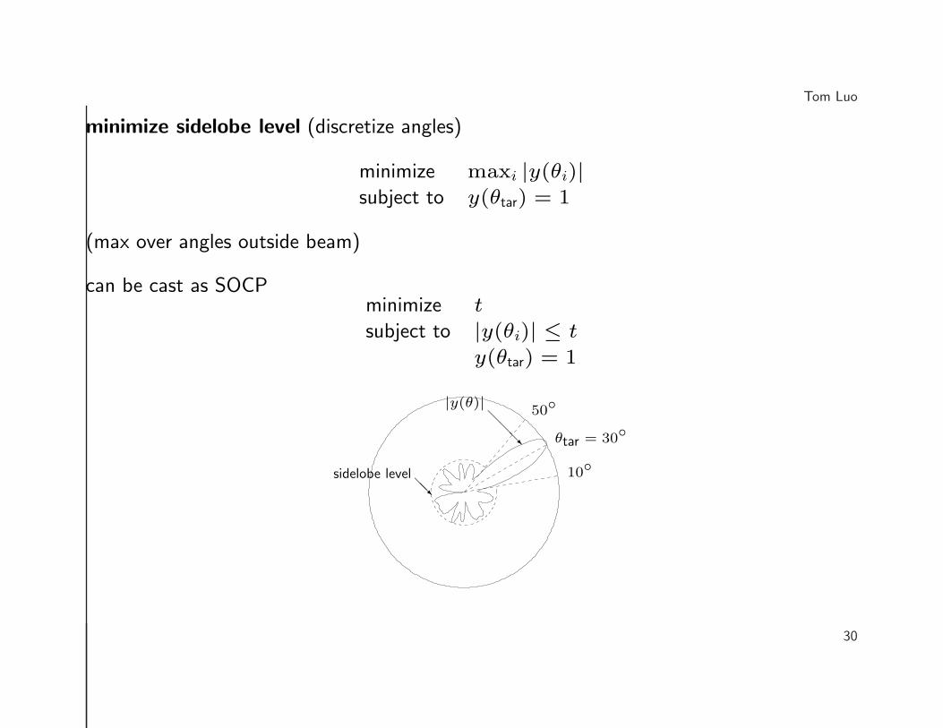
minimize sidelobe level (discretize angles)
minimize maxi |y(θi)|subject to y(θtar) = 1
(max over angles outside beam)
can be cast as SOCPminimize t
subject to |y(θi)| ≤ t
y(θtar) = 1
θtar = 30◦50◦
10◦
@@@R
|y(θ)|
@@Rsidelobe level
30
Tom Luo
Other variants
convex (& quasiconvex) extensions:
• y(θ0) = 0 (null in direction θ0)
• w is real (amplitude only shading)
• |wi| ≤ 1 (attenuation only shading)
• minimize σ2∑ni=1 |wi|2 (thermal noise power in y)
• minimize beamwidth given a maximum sidelobe level
nonconvex extension:
• maximize number of zero weights
31
Tom Luo
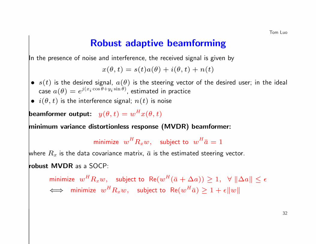
Robust adaptive beamforming
In the presence of noise and interference, the received signal is given by
x(θ, t) = s(t)a(θ) + i(θ, t) + n(t)
• s(t) is the desired signal, a(θ) is the steering vector of the desired user; in the ideal
case a(θ) = ej(xi cos θ+yi sin θ), estimated in practice
• i(θ, t) is the interference signal; n(t) is noise
beamformer output: y(θ, t) = wHx(θ, t)
minimum variance distortionless response (MVDR) beamformer:
minimize wHRxw, subject to wHa = 1
where Rx is the data covariance matrix, a is the estimated steering vector.
robust MVDR as a SOCP:
minimize wHRxw, subject to Re(wH(a + ∆a)) ≥ 1, ∀ ‖∆a‖ ≤ ε
⇐⇒ minimize wHRxw, subject to Re(wHa) ≥ 1 + ε‖w‖
32

Tom Luo
Optimal receiver location
N transmitter frequencies 1, . . . , N
transmitters @ ai, bi use frequency i (ai, bi ∈ R2)
transmitters @ a1, a2, . . . , aN are wanted
transmitters @ b1, b2, . . . , bN are interfering
x
q
b1
q
b2
q
b3
a
a1
a
a2
a
a3
(signal) receiver power from ai: ‖x − ai‖−α
(interfering) receiver power from bi: ‖x − bi‖−α (α ≈ 2.1)
worst signal to interference ratio as a function of receiver position x:
S/I = mini
‖x − ai‖−α
‖x − bi‖−α
what is the optimal receiver location?
33
Tom Luo
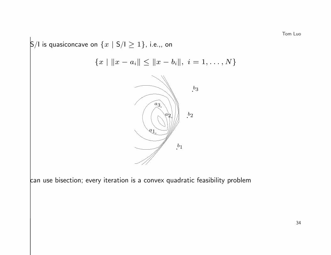
S/I is quasiconcave on {x | S/I ≥ 1}, i.e.,, on
{x | ‖x − ai‖ ≤ ‖x − bi‖, i = 1, . . . , N}
q
b1
q
b2
q
b3
a
a1
a
a2
a
a3
can use bisection; every iteration is a convex quadratic feasibility problem
34