Time series models: sparse estimation and robustness aspects
164
Time series models: sparse estimation and robustness aspects Christophe Croux (KU Leuven, Belgium) 2017 CRonos Spring Course Limassol, Cyprus, 8-10 April Based on joint work with Ines Wilms, Ruben Crevits, and Sarah Gelper.
Transcript of Time series models: sparse estimation and robustness aspects
Time series models: sparse estimation and
robustness aspects
Christophe Croux (KU Leuven, Belgium)
2017 CRonos Spring Course
Limassol, Cyprus, 8-10 April
Based on joint work with Ines Wilms, Ruben Crevits, and Sarah Gelper.

Part I
Autoregressive models: from one timeseries to many time series
2 / 164

Outline
1 Univariate
2 Multivariate
3 Big Data
3 / 164

Univariate
Section 1
Univariate
4 / 164
Univariate
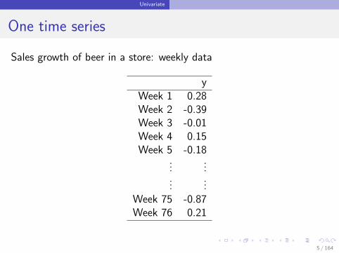
One time series
Sales growth of beer in a store: weekly data
yWeek 1 0.28Week 2 -0.39Week 3 -0.01Week 4 0.15Week 5 -0.18
......
......
Week 75 -0.87Week 76 0.21
5 / 164
Univariate
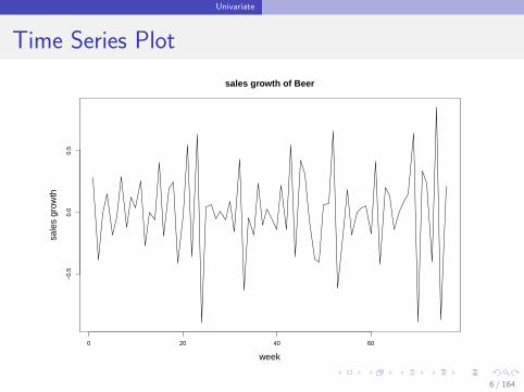
Time Series Plot
0 20 40 60
−0.
50.
00.
5
sales growth of Beer
week
sale
s gr
owth
6 / 164
Univariate
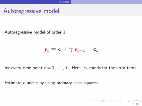
Autoregressive model
Autoregressive model of order 1:
yt = c + γ yt−1 + et
for every time point t = 1, . . . ,T . Here, et stands for the error term.
Estimate c and γ by using ordinary least squares.
7 / 164
Univariate
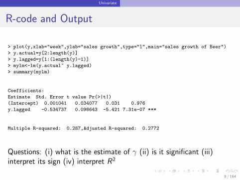
R-code and Output
> plot(y,xlab="week",ylab="sales growth",type="l",main="sales growth of Beer")
> y.actual=y[2:length(y)]
> y.lagged=y[1:(length(y)-1)]
> mylm<-lm(y.actual~ y.lagged)
> summary(mylm)
Coefficients:
Estimate Std. Error t value Pr(>|t|)
(Intercept) 0.001041 0.034077 0.031 0.976
y.lagged -0.534737 0.098643 -5.421 7.31e-07 ***
Multiple R-squared: 0.287,Adjusted R-squared: 0.2772
Questions: (i) what is the estimate of γ (ii) is it significant (iii)interpret its sign (iv) interpret R2
8 / 164
Univariate
Forecasting
Using the observations y1, y2, . . . , yT we forecast the next observationuisng the formula
yT+1 = c + γ yT
Can we also forecast at horizon 2 ? YES
yT+2 = c + γ yT+1
9 / 164
Univariate
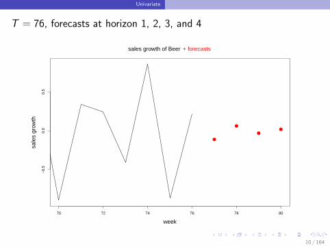
T = 76, forecasts at horizon 1, 2, 3, and 4
70 72 74 76 78 80
−0.
50.
00.
5
week
sale
s gr
owth
sales growth of Beer + forecasts
10 / 164

Multivariate
Section 2
Multivariate
11 / 164

Multivariate
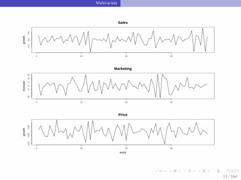
3 time series
Predict next week sales using the observed
Sales
+ additional information, like
Price
Marketing Effort
Three stationary time series y1,t , y2,t , and y3,t .
12 / 164
Multivariate
0 20 40 60
−0.
50.
00.
5
Salesgr
owth
0 20 40 60
−15
−5
05
1015
Marketing
incr
ease
0 20 40 60
−0.
15−
0.05
0.05
Price
week
grow
th
13 / 164
Multivariate
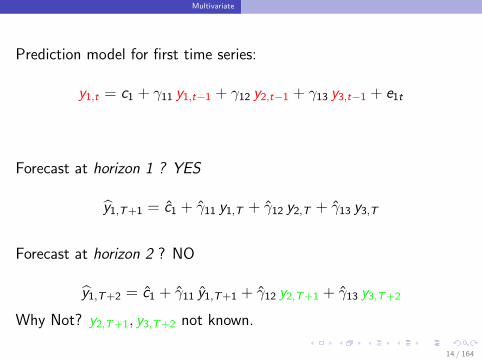
Prediction model for first time series:
y1,t = c1 + γ11 y1,t−1 + γ12 y2,t−1 + γ13 y3,t−1 + e1t
Forecast at horizon 1 ? YES
y1,T+1 = c1 + γ11 y1,T + γ12 y2,T + γ13 y3,T
Forecast at horizon 2 ? NO
y1,T+2 = c1 + γ11 y1,T+1 + γ12 y2,T+1 + γ13 y3,T+2
Why Not? y2,T+1, y3,T+2 not known.
14 / 164
Multivariate
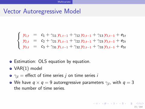
Vector Autoregressive Model
y1,t = c1 + γ11 y1,t−1 + γ12 y2,t−1 + γ13 y3,t−1 + e1t
y2,t = c2 + γ21 y1,t−1 + γ22 y2,t−1 + γ23 y3,t−1 + e2t
y3,t = c3 + γ31 y1,t−1 + γ32 y2,t−1 + γ33 y3,t−1 + e3t
Estimation: OLS equation by equation.
VAR(1) model
γji = effect of time series j on time series i
We have q × q = 9 autoregressive parameters γji , with q = 3the number of time series.
15 / 164
Multivariate
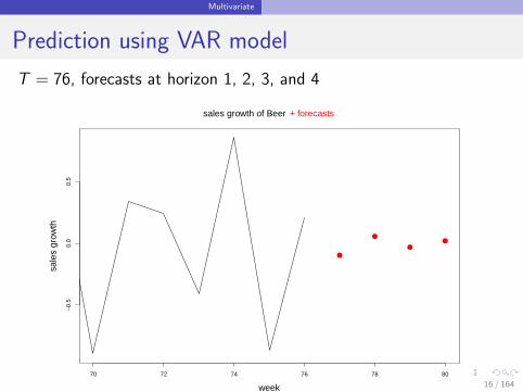
Prediction using VAR model
T = 76, forecasts at horizon 1, 2, 3, and 4
70 72 74 76 78 80
−0.
50.
00.
5
week
sale
s gr
owth
sales growth of Beer + forecasts
16 / 164

Big Data
Section 3
Big Data
17 / 164

Big Data
Many time series
Predict next week sales of Beer using the observed
Sales of Beer
+
Price of Beer
Marketing Effort for Beer
+
Prices of other product categories
Marketing Effort for other product categories
Vector Autoregressive model ≡ Market Response Model
18 / 164
Big Data
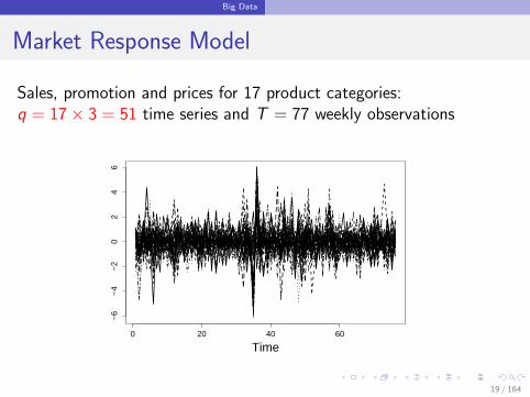
Market Response Model
Sales, promotion and prices for 17 product categories:q = 17× 3 = 51 time series and T = 77 weekly observations
0 20 40 60
−6
−4
−2
02
46
Time
19 / 164
Big Data
VAR model for q = 3× 17 = 51 time series
q × q = 2601 autoregressive parameters
→ Explosion of number of parameters
Use the LASSO instead of OLS.
Question: Why?
20 / 164

Big Data
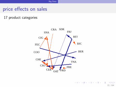
Network
Network with q nodes. Each node corresponds with a time series.
draw an edge from node i to node j if
γji 6= 0
the edge width is the size of the effect
the edge color is the sign of the effect(blue if positive, red if negative)
21 / 164
Big Data
price effects on sales
17 product categories
BER
BJC
RFJ
FRJSDRCRA
SNA
CIG
FEC
COO
CHE
CSO
CEROAT FRD
FRE
TNA
22 / 164

Big Data
23 / 164

Part II
Basic time series concepts
24 / 164

Outline
1 Stationarity
2 Autocorrelation
3 Differencing
4 AR and MA Models
5 MA-infinity representation
25 / 164

Stationarity
Section 1
Stationarity
26 / 164
Stationarity
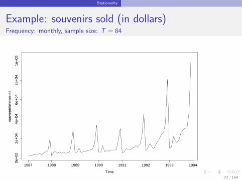
Example: souvenirs sold (in dollars)Frequency: monthly, sample size: T = 84
Time
souv
enir
times
erie
s
1987 1988 1989 1990 1991 1992 1993 1994
0e+
002e
+04
4e+
046e
+04
8e+
041e
+05
27 / 164
Stationarity
Stochastic Process
A Stochastic Process is a sequence of stochastic variables:. . . ,Y1,Y2,Y3, . . . ,YT . . .. We observe the process from t = 1 tot = T , yielding a sequence of numbers
y1, y2, y3, . . . , yT
which we call a time series.
We only treat regularly spaced, discrete time series. Note that theobservations in a time series are not independent! We need to rely onthe concept of stationarity.
28 / 164

Stationarity
Stationarity
We say that a stochastic process is (weakly) stationary if
1 E [Yt ] is the same for all t
2 Var[Yt ] is the same for all t
3 Cov(Yt ,Yt−k) is the same for all t, for every k > 0.
29 / 164

Autocorrelation
Section 2
Autocorrelation
30 / 164
Autocorrelation
Autocorrelations
Then we define the autocorrelation of order k as
ρk = Corr(Yt ,Yt−k) =Cov(Yt ,Yt−k)
Var[Yt ].
The autocorrelations give insight in the dependency structure of theprocess.The autocorrelations can be estimated by
ρk =
∑Tt=k+1(yt − y)(yt−k − y)∑T
t=1(yt − y)2.
31 / 164

Autocorrelation
The correlogram
A plot of ρk versus k is called a correlogram. On a correlogram, weoften see 2 lines, corresponding to the critical values of the teststatistic
√T ρk for testing H0 : ρk = 0 for a specific value of k .
32 / 164
Autocorrelation
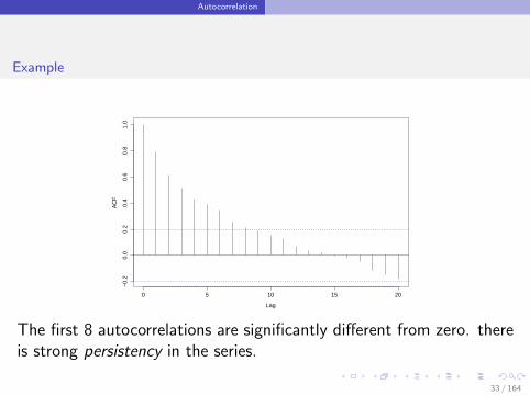
Example
0 5 10 15 20
−0.
20.
00.
20.
40.
60.
81.
0
Lag
AC
F
The first 8 autocorrelations are significantly different from zero. thereis strong persistency in the series.
33 / 164

Differencing
Section 3
Differencing
34 / 164
Differencing
Difference Operators
The “Lag” operator L is defined as
LYt = Yt−1.
Note that LsYt = Yt−s .
The difference operator ∆ is defined as
∆Yt = (I − L)Yt = Yt − Yt−1.
Linear trends can be eliminated by applying ∆ once. If a stationaryprocess is then obtained, we say that Yt is integrated of order 1.
35 / 164
Differencing
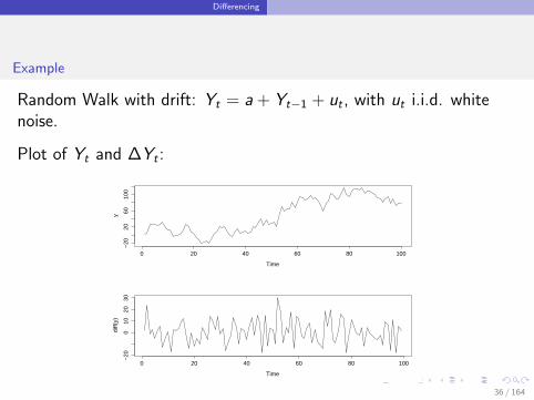
Example
Random Walk with drift: Yt = a + Yt−1 + ut , with ut i.i.d. whitenoise.
Plot of Yt and ∆Yt :
Time
y
0 20 40 60 80 100
−20
2060
100
Time
diff(
y)
0 20 40 60 80 100
−20
010
2030
36 / 164
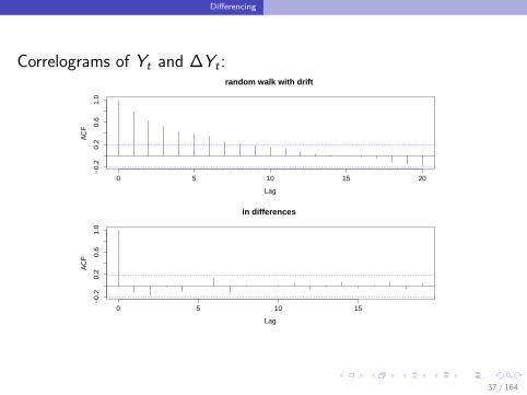
Differencing
Correlograms of Yt and ∆Yt :
0 5 10 15 20
−0.
20.
20.
61.
0
Lag
AC
Frandom walk with drift
0 5 10 15
−0.
20.
20.
61.
0
Lag
AC
F
in differences
37 / 164
Differencing
Seasonality
Seasonal effects of order s can be eliminated by applying thedifference operator of order s:
∆sYt = (I − Ls)Yt = Yt − Yt−s
s = 12, monthly data
s = 4, quarterly data
Note than one loses s observations when differencing.
38 / 164
Differencing
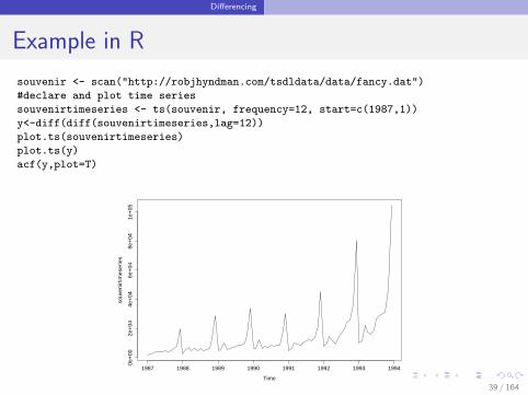
Example in R
souvenir <- scan("http://robjhyndman.com/tsdldata/data/fancy.dat")
#declare and plot time series
souvenirtimeseries <- ts(souvenir, frequency=12, start=c(1987,1))
y<-diff(diff(souvenirtimeseries,lag=12))
plot.ts(souvenirtimeseries)
plot.ts(y)
acf(y,plot=T)
Time
souv
enir
times
erie
s
1987 1988 1989 1990 1991 1992 1993 1994
0e+
002e
+04
4e+
046e
+04
8e+
041e
+05
39 / 164
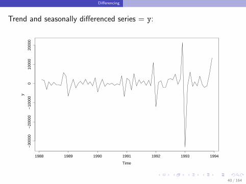
Differencing
Trend and seasonally differenced series = y:
Time
y
1988 1989 1990 1991 1992 1993 1994
−30
000
−20
000
−10
000
010
000
2000
0
40 / 164
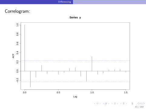
Differencing
Correlogram:
0.0 0.5 1.0 1.5
−0.
20.
00.
20.
40.
60.
81.
0
Lag
AC
F
Series y
41 / 164

AR and MA Models
Section 4
AR and MA Models
42 / 164
AR and MA Models
White Noise
A white noise process is a sequence of i.i.d. observations with zeromean and variance σ2 and we will denote it by ut .
It is the building block of more complicated processes:For example, a random walk (without drift) model Yt is defined by∆Yt = ut , or Yt = Yt−1 + ut .
ut is sometimes called the innovation process. It is not predictable.
43 / 164
AR and MA Models
Why do we need models?
To describe parsimoneously the dynamics of the time series.
For forecasting. For example:
Take a random walk model: Yt+1 = Yt + ut+1 for every t. Recallthat T is the last observation, then
YT+h = YT ,
for every forecast horizon h.
44 / 164
AR and MA Models
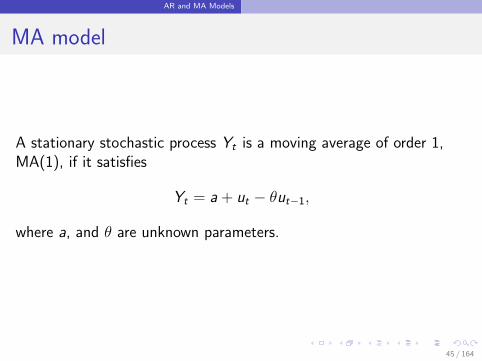
MA model
A stationary stochastic process Yt is a moving average of order 1,MA(1), if it satisfies
Yt = a + ut − θut−1,
where a, and θ are unknown parameters.
45 / 164

AR and MA Models
The autocorrelations of an MA(1) are given by
ρ0 = 1
ρ1 = Corr(Yt ,Yt−1) = − θ(1+θ2)
ρ2 = 0
ρ3 = 0
...
46 / 164
AR and MA Models
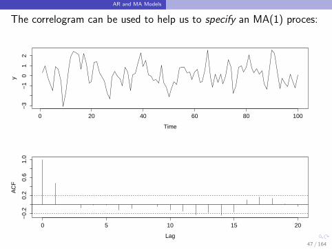
The correlogram can be used to help us to specify an MA(1) proces:
Time
y
0 20 40 60 80 100
−3
−1
01
2
0 5 10 15 20
−0.
20.
20.
61.
0
Lag
AC
F
47 / 164
AR and MA Models
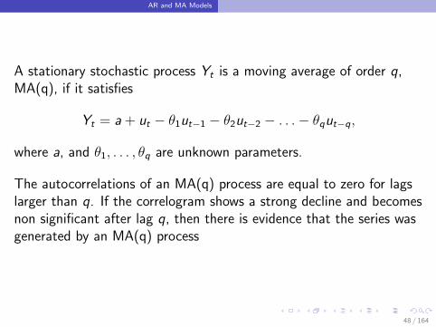
A stationary stochastic process Yt is a moving average of order q,MA(q), if it satisfies
Yt = a + ut − θ1ut−1 − θ2ut−2 − . . .− θqut−q,
where a, and θ1, . . . , θq are unknown parameters.
The autocorrelations of an MA(q) process are equal to zero for lagslarger than q. If the correlogram shows a strong decline and becomesnon significant after lag q, then there is evidence that the series wasgenerated by an MA(q) process
48 / 164
AR and MA Models
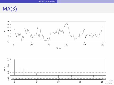
MA(3)
Time
y
0 20 40 60 80 100
−3
−1
12
34
0 5 10 15 20
−0.
20.
20.
61.
0
Lag
AC
F
49 / 164
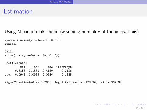
AR and MA Models
Estimation
Using Maximum Likelihood (assuming normality of the innovations)
mymodel<-arima(y,order=c(0,0,3))
mymodel
Call:
arima(x = y, order = c(0, 0, 3))
Coefficients:
ma1 ma2 ma3 intercept
0.5158 0.1880 0.4150 0.0126
s.e. 0.0948 0.0935 0.0936 0.1835
sigma^2 estimated as 0.765: log likelihood = -128.96, aic = 267.92
50 / 164
AR and MA Models
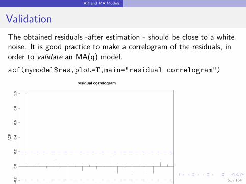
Validation
The obtained residuals -after estimation - should be close to a whitenoise. It is good practice to make a correlogram of the residuals, inorder to validate an MA(q) model.
acf(mymodel$res,plot=T,main="residual correlogram")
0 5 10 15 20
−0.
20.
00.
20.
40.
60.
81.
0
Lag
AC
F
residual correlogram
51 / 164
AR and MA Models
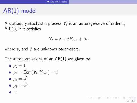
AR(1) model
A stationary stochastic process Yt is an autoregressive of order 1,AR(1), if it satisfies
Yt = a + φYt−1 + ut ,
where a, and φ are unknown parameters.
The autocorrelations of an AR(1) are given by
ρ0 = 1
ρ1 = Corr(Yt ,Yt−1) = φ
ρ2 = φ2
ρ3 = φ3
...
52 / 164
AR and MA Models
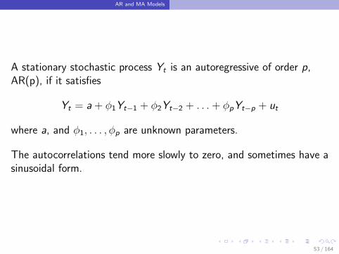
A stationary stochastic process Yt is an autoregressive of order p,AR(p), if it satisfies
Yt = a + φ1Yt−1 + φ2Yt−2 + . . . + φpYt−p + ut
where a, and φ1, . . . , φp are unknown parameters.
The autocorrelations tend more slowly to zero, and sometimes have asinusoidal form.
53 / 164
AR and MA Models
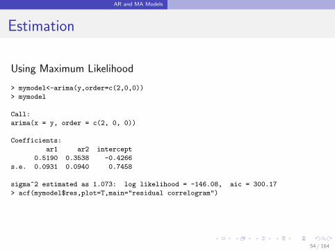
Estimation
Using Maximum Likelihood
> mymodel<-arima(y,order=c(2,0,0))
> mymodel
Call:
arima(x = y, order = c(2, 0, 0))
Coefficients:
ar1 ar2 intercept
0.5190 0.3538 -0.4266
s.e. 0.0931 0.0940 0.7458
sigma^2 estimated as 1.073: log likelihood = -146.08, aic = 300.17
> acf(mymodel$res,plot=T,main="residual correlogram")
54 / 164
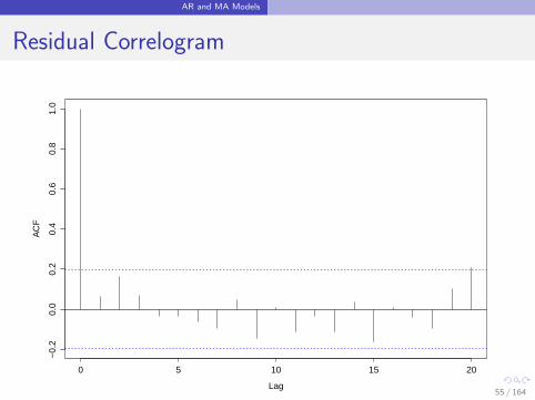
AR and MA Models
Residual Correlogram
0 5 10 15 20
−0.
20.
00.
20.
40.
60.
81.
0
Lag
AC
F
55 / 164

MA-infinity representation
Section 5
MA-infinity representation
56 / 164
MA-infinity representation
Wold Representation Theorem
If Yt is a stationary process, then it can be written as an MA(∞):
Yt = c + ut ++∞∑k=1
θkut−k for any t.
57 / 164
MA-infinity representation
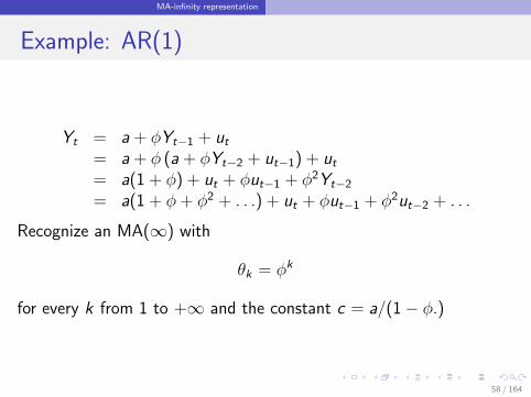
Example: AR(1)
Yt = a + φYt−1 + ut= a + φ (a + φYt−2 + ut−1) + ut= a(1 + φ) + ut + φut−1 + φ2Yt−2
= a(1 + φ + φ2 + . . .) + ut + φut−1 + φ2ut−2 + . . .
Recognize an MA(∞) with
θk = φk
for every k from 1 to +∞ and the constant c = a/(1− φ.)
58 / 164
MA-infinity representation
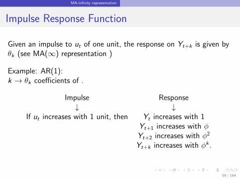
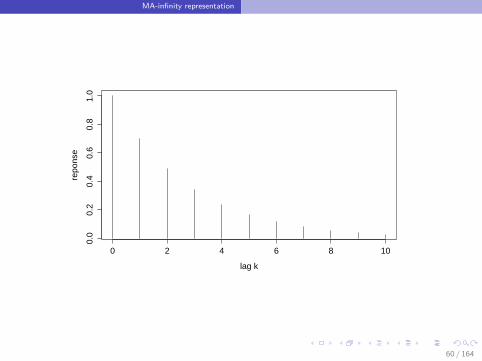
Impulse Response Function
Given an impulse to ut of one unit, the response on Yt+k is given byθk (see MA(∞) representation )
Example: AR(1):k → θk coefficients of .
Impulse Response↓ ↓
If ut increases with 1 unit, then Yt increases with 1Yt+1 increases with φYt+2 increases with φ2
Yt+k increases with φk .
59 / 164
MA-infinity representation
0 2 4 6 8 10
0.0
0.2
0.4
0.6
0.8
1.0
lag k
repo
nse
60 / 164

Part III
Introduction to dynamic models
61 / 164

Outline
1 Example
2 Granger Causality
3 Vector Autoregressive Model
62 / 164

Example
Section 1
Example
63 / 164
Example
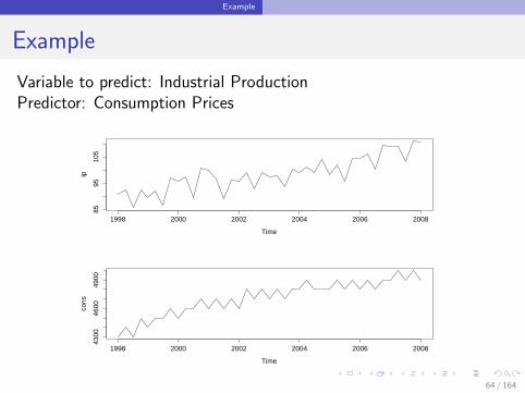
Example
Variable to predict: Industrial ProductionPredictor: Consumption Prices
Time
ip
1998 2000 2002 2004 2006 2008
8595
105
Time
cons
1998 2000 2002 2004 2006 2008
4300
4600
4900
64 / 164
Example
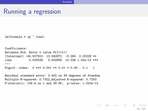
Running a regression
lm(formula = ip ~ cons)
Coefficients:
Estimate Std. Error t value Pr(>|t|)
(Intercept) -45.507915 13.940872 -3.264 0.00229 **
cons 0.030528 0.002956 10.326 1.02e-12 ***
---
Signif. codes: 0 *** 0.001 ** 0.01 * 0.05 . 0.1 1
Residual standard error: 3.402 on 39 degrees of freedom
Multiple R-squared: 0.7322,Adjusted R-squared: 0.7253
F-statistic: 106.6 on 1 and 39 DF, p-value: 1.022e-12
65 / 164
Example
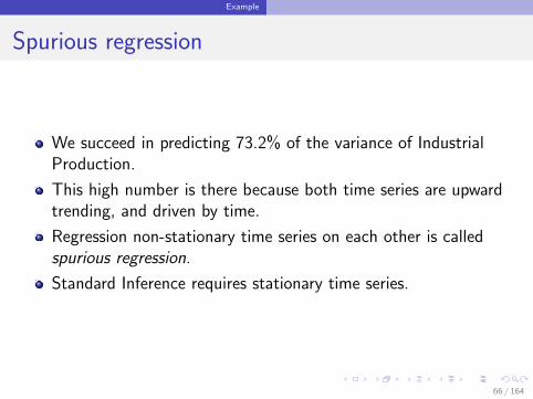
Spurious regression
We succeed in predicting 73.2% of the variance of IndustrialProduction.
This high number is there because both time series are upwardtrending, and driven by time.
Regression non-stationary time series on each other is calledspurious regression.
Standard Inference requires stationary time series.
66 / 164
Example
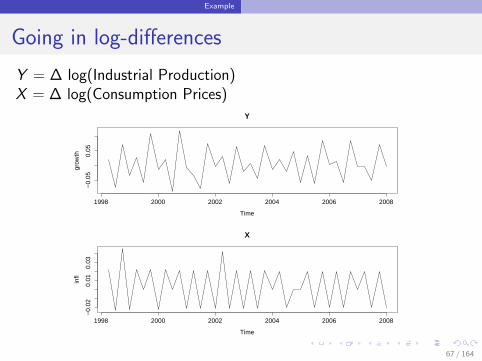
Going in log-differences
Y = ∆ log(Industrial Production)X = ∆ log(Consumption Prices)
Y
Time
grow
th
1998 2000 2002 2004 2006 2008
−0.
050.
05
X
Time
infl
1998 2000 2002 2004 2006 2008
−0.
020.
010.
03
67 / 164
Example
Note that
∆ log(Xt) = log(Xt)− log(Xt−1) = log(Xt/Xt−1) ≈ Xt − Xt−1
Xt−1.
We get relative differences, or percentagewise increments.
Y = ∆ log(Industrial Production) = GrowthX = ∆ log(Consumption Prices) = Inflation
68 / 164
Example
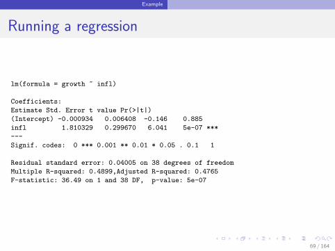
Running a regression
lm(formula = growth ~ infl)
Coefficients:
Estimate Std. Error t value Pr(>|t|)
(Intercept) -0.000934 0.006408 -0.146 0.885
infl 1.810329 0.299670 6.041 5e-07 ***
---
Signif. codes: 0 *** 0.001 ** 0.01 * 0.05 . 0.1 1
Residual standard error: 0.04005 on 38 degrees of freedom
Multiple R-squared: 0.4899,Adjusted R-squared: 0.4765
F-statistic: 36.49 on 1 and 38 DF, p-value: 5e-07
69 / 164
Example
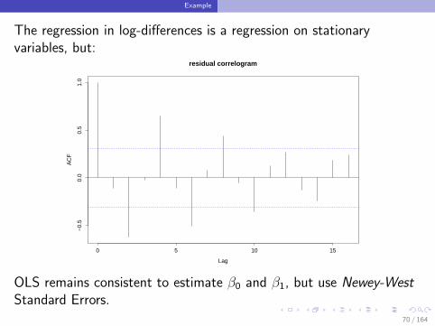
The regression in log-differences is a regression on stationaryvariables, but:
0 5 10 15
−0.
50.
00.
51.
0
Lag
AC
Fresidual correlogram
OLS remains consistent to estimate β0 and β1, but use Newey-WestStandard Errors.
70 / 164

Granger Causality
Section 2
Granger Causality
71 / 164
Granger Causality
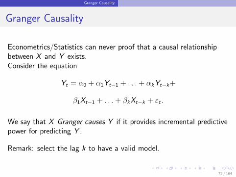
Granger Causality
Econometrics/Statistics can never proof that a causal relationshipbetween X and Y exists.Consider the equation
Yt = α0 + α1Yt−1 + . . . + αkYt−k+
β1Xt−1 + . . . + βkXt−k + εt .
We say that X Granger causes Y if it provides incremental predictivepower for predicting Y .
Remark: select the lag k to have a valid model.
72 / 164
Granger Causality
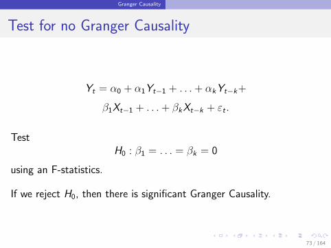
Test for no Granger Causality
Yt = α0 + α1Yt−1 + . . . + αkYt−k+
β1Xt−1 + . . . + βkXt−k + εt .
TestH0 : β1 = . . . = βk = 0
using an F-statistics.
If we reject H0, then there is significant Granger Causality.
73 / 164
Granger Causality
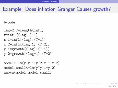
Example: Does inflation Granger Causes growth?
R-code
lag=2;T=length(infl)
x=infl[(lag+1):T]
x.1=infl[(lag):(T-1)]
x.2=infl[(lag-1):(T-2)]
y.1=growth[(lag):(T-1)]
y.2=growth[(lag-1):(T-2)]
model<-lm(y~y.1+y.2+x.1+x.2)
model.small<-lm(y~y.1+y.2)
anova(model,model.small)
74 / 164
Granger Causality
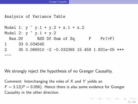
Analysis of Variance Table
Model 1: y ~ y.1 + y.2 + x.1 + x.2
Model 2: y ~ y.1 + y.2
Res.Df RSS Df Sum of Sq F Pr(>F)
1 33 0.034545
2 35 0.066910 -2 -0.032365 15.459 1.831e-05 ***
---
We strongly reject the hypothesis of no Granger Causality.
Comment: Interchanging the roles of X and Y yields an
F = 3.12(P = 0.056). Hence there is also some evidence for Granger
Causality in the other direction.
75 / 164

Vector Autoregressive Model
Section 3
Vector Autoregressive Model
76 / 164
Vector Autoregressive Model
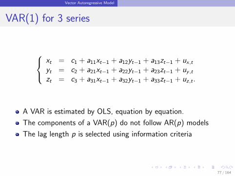
VAR(1) for 3 series
xt = c1 + a11xt−1 + a12yt−1 + a13zt−1 + ux ,tyt = c2 + a21xt−1 + a22yt−1 + a23zt−1 + uy ,tzt = c3 + a31xt−1 + a32yt−1 + a33zt−1 + uz,t .
A VAR is estimated by OLS, equation by equation.
The components of a VAR(p) do not follow AR(p) models
The lag length p is selected using information criteria
77 / 164
Vector Autoregressive Model
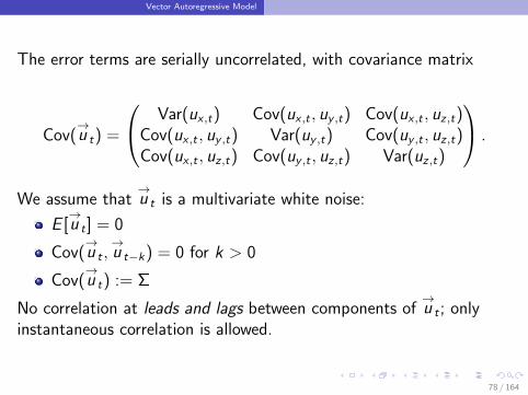
The error terms are serially uncorrelated, with covariance matrix
Cov(→u t) =
Var(ux ,t) Cov(ux ,t , uy ,t) Cov(ux ,t , uz,t)Cov(ux ,t , uy ,t) Var(uy ,t) Cov(uy ,t , uz,t)Cov(ux ,t , uz,t) Cov(uy ,t , uz,t) Var(uz,t)
.
We assume that→u t is a multivariate white noise:
E [→u t ] = 0
Cov(→u t ,
→u t−k) = 0 for k > 0
Cov(→u t) := Σ
No correlation at leads and lags between components of→u t ; only
instantaneous correlation is allowed.
78 / 164

Vector Autoregressive Model
Impulse-response functions:
If component i of the innovation→u t changes with one-unit, then
component j of→y t+k changes with (Bk)ji (other things equal).
The functionk → (Bk)ji
is called the impulse-response function.
There are k2 impulse response functions.
[There exists many variants of the impulse response functions.]
79 / 164
Vector Autoregressive Model
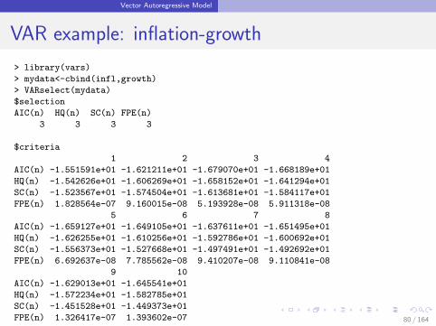
VAR example: inflation-growth
> library(vars)
> mydata<-cbind(infl,growth)
> VARselect(mydata)
$selection
AIC(n) HQ(n) SC(n) FPE(n)
3 3 3 3
$criteria
1 2 3 4
AIC(n) -1.551591e+01 -1.621211e+01 -1.679070e+01 -1.668189e+01
HQ(n) -1.542626e+01 -1.606269e+01 -1.658152e+01 -1.641294e+01
SC(n) -1.523567e+01 -1.574504e+01 -1.613681e+01 -1.584117e+01
FPE(n) 1.828564e-07 9.160015e-08 5.193928e-08 5.911318e-08
5 6 7 8
AIC(n) -1.659127e+01 -1.649105e+01 -1.637611e+01 -1.651495e+01
HQ(n) -1.626255e+01 -1.610256e+01 -1.592786e+01 -1.600692e+01
SC(n) -1.556373e+01 -1.527668e+01 -1.497491e+01 -1.492692e+01
FPE(n) 6.692637e-08 7.785562e-08 9.410207e-08 9.110841e-08
9 10
AIC(n) -1.629013e+01 -1.645541e+01
HQ(n) -1.572234e+01 -1.582785e+01
SC(n) -1.451528e+01 -1.449373e+01
FPE(n) 1.326417e-07 1.393602e-07 80 / 164
Vector Autoregressive Model
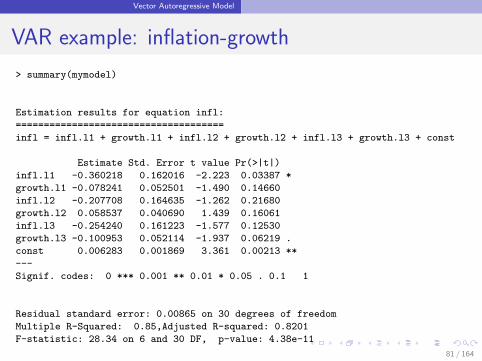
VAR example: inflation-growth
> summary(mymodel)
Estimation results for equation infl:
=====================================
infl = infl.l1 + growth.l1 + infl.l2 + growth.l2 + infl.l3 + growth.l3 + const
Estimate Std. Error t value Pr(>|t|)
infl.l1 -0.360218 0.162016 -2.223 0.03387 *
growth.l1 -0.078241 0.052501 -1.490 0.14660
infl.l2 -0.207708 0.164635 -1.262 0.21680
growth.l2 0.058537 0.040690 1.439 0.16061
infl.l3 -0.254240 0.161223 -1.577 0.12530
growth.l3 -0.100953 0.052114 -1.937 0.06219 .
const 0.006283 0.001869 3.361 0.00213 **
---
Signif. codes: 0 *** 0.001 ** 0.01 * 0.05 . 0.1 1
Residual standard error: 0.00865 on 30 degrees of freedom
Multiple R-Squared: 0.85,Adjusted R-squared: 0.8201
F-statistic: 28.34 on 6 and 30 DF, p-value: 4.38e-11
81 / 164
Vector Autoregressive Model
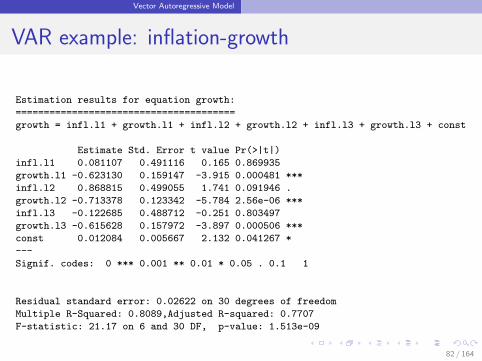
VAR example: inflation-growth
Estimation results for equation growth:
=======================================
growth = infl.l1 + growth.l1 + infl.l2 + growth.l2 + infl.l3 + growth.l3 + const
Estimate Std. Error t value Pr(>|t|)
infl.l1 0.081107 0.491116 0.165 0.869935
growth.l1 -0.623130 0.159147 -3.915 0.000481 ***
infl.l2 0.868815 0.499055 1.741 0.091946 .
growth.l2 -0.713378 0.123342 -5.784 2.56e-06 ***
infl.l3 -0.122685 0.488712 -0.251 0.803497
growth.l3 -0.615628 0.157972 -3.897 0.000506 ***
const 0.012084 0.005667 2.132 0.041267 *
---
Signif. codes: 0 *** 0.001 ** 0.01 * 0.05 . 0.1 1
Residual standard error: 0.02622 on 30 degrees of freedom
Multiple R-Squared: 0.8089,Adjusted R-squared: 0.7707
F-statistic: 21.17 on 6 and 30 DF, p-value: 1.513e-09
Covariance matrix of residuals:
infl growth
infl 7.482e-05 0.0000499
growth 4.990e-05 0.0006875
Correlation matrix of residuals:
infl growth
infl 1.00 0.22
growth 0.22 1.00
82 / 164
Vector Autoregressive Model
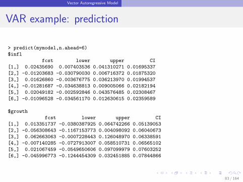
VAR example: prediction
> predict(mymodel,n.ahead=6)
$infl
fcst lower upper CI
[1,] 0.02435690 0.007403536 0.041310271 0.01695337
[2,] -0.01203683 -0.030790030 0.006716372 0.01875320
[3,] 0.01626860 -0.003676775 0.036213970 0.01994537
[4,] -0.01281687 -0.034638813 0.009005066 0.02182194
[5,] 0.02049182 -0.002592846 0.043576485 0.02308467
[6,] -0.01096528 -0.034561170 0.012630615 0.02359589
$growth
fcst lower upper CI
[1,] 0.013351737 -0.0380387925 0.064742266 0.05139053
[2,] -0.056308643 -0.1167153773 0.004098092 0.06040673
[3,] 0.062663063 -0.0007228443 0.126048970 0.06338591
[4,] -0.007140285 -0.0727913007 0.058510731 0.06565102
[5,] 0.021067459 -0.0549650606 0.097099979 0.07603252
[6,] -0.045996773 -0.1244454309 0.032451885 0.07844866
83 / 164
Vector Autoregressive Model
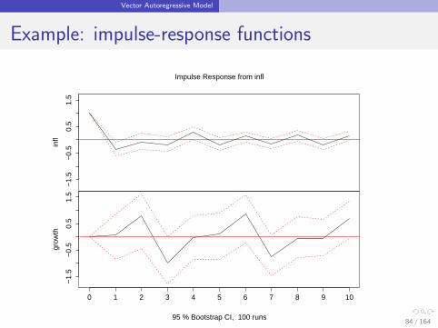
Example: impulse-response functions
xy$x
infl
−1.
5−
0.5
0.5
1.5
xy$x
grow
th
−1.
5−
0.5
0.5
1.5
0 1 2 3 4 5 6 7 8 9 10
Impulse Response from infl
95 % Bootstrap CI, 100 runs84 / 164
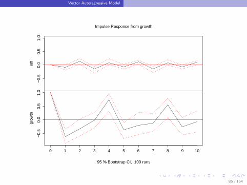
Vector Autoregressive Model
xy$x
infl
−0.
50.
00.
51.
0
xy$x
grow
th
−0.
50.
00.
51.
0
0 1 2 3 4 5 6 7 8 9 10
Impulse Response from growth
95 % Bootstrap CI, 100 runs
85 / 164

Part IV
Sparse Cointegration
86 / 164

Outline
1 Introduction
2 Penalized Estimation
3 Forecasting Applications
87 / 164

Introduction
Section 1
Introduction
88 / 164
Introduction
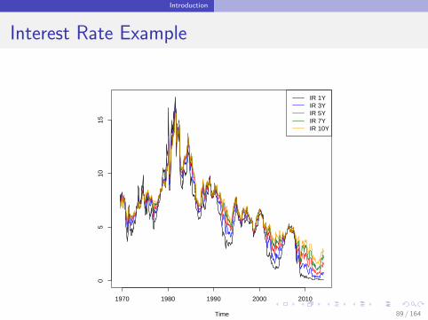
Interest Rate Example
Time
1970 1980 1990 2000 2010
05
1015
IR 1YIR 3YIR 5YIR 7YIR 10Y
89 / 164
Introduction
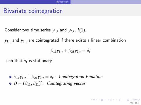
Bivariate cointegration
Consider two time series y1,t and y2,t , I (1).
y1,t and y2,t are cointegrated if there exists a linear combination
β11y1,t + β21y2,t = δt
such that δt is stationary.
β11y1,t + β21y2,t = δt : Cointegration Equation
β = (β11, β21)′ : Cointegrating vector
90 / 164
Introduction
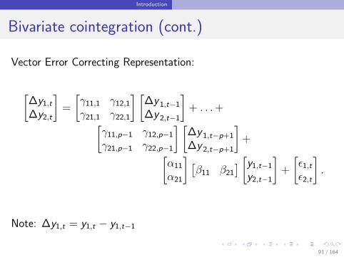
Bivariate cointegration (cont.)
Vector Error Correcting Representation:
[∆y1,t
∆y2,t
]=
[γ11,1 γ12,1
γ21,1 γ22,1
] [∆y 1,t−1
∆y 2,t−1
]+ . . .+[
γ11,p−1 γ12,p−1
γ21,p−1 γ22,p−1
] [∆y 1,t−p+1
∆y 2,t−p+1
]+[
α11
α21
] [β11 β21
] [y1,t−1
y2,t−1
]+
[ε1,t
ε2,t
].
Note: ∆y1,t = y1,t − y1,t−1
91 / 164
Introduction
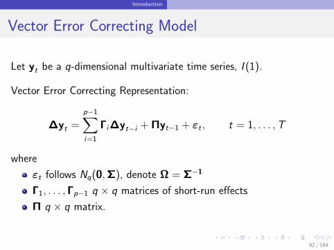
Vector Error Correcting Model
Let yt be a q-dimensional multivariate time series, I (1).
Vector Error Correcting Representation:
∆yt =
p−1∑i=1
Γi∆yt−i + Πyt−1 + εt , t = 1, . . . ,T
where
εt follows Nq(0,Σ), denote Ω = Σ−1
Γ1, . . . ,Γp−1 q × q matrices of short-run effects
Π q × q matrix.
92 / 164
Introduction
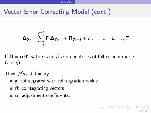
Vector Error Correcting Model (cont.)
∆yt =
p−1∑i=1
Γi∆yt−i + Πyt−1 + εt . t = 1, . . . ,T
If Π = αβ′, with α and β q × r matrices of full column rank r(r < q)
Then, β′yt stationary
yt cointegrated with cointegration rank r
β: cointegrating vectors
α: adjustment coefficients.
93 / 164
Introduction
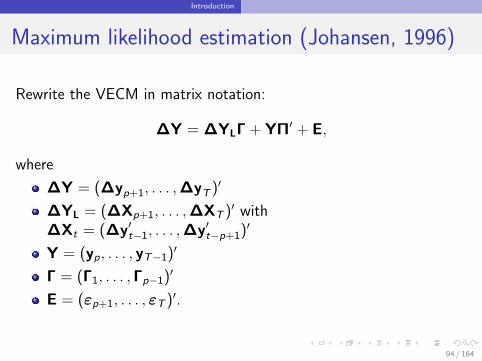
Maximum likelihood estimation (Johansen, 1996)
Rewrite the VECM in matrix notation:
∆Y = ∆YLΓ + YΠ′ + E,
where
∆Y = (∆yp+1, . . . ,∆yT )′
∆YL = (∆Xp+1, . . . ,∆XT )′ with∆Xt = (∆y′t−1, . . . ,∆y′t−p+1)′
Y = (yp, . . . , yT−1)′
Γ = (Γ1, . . . ,Γp−1)′
E = (εp+1, . . . , εT )′.
94 / 164
Introduction
Maximum likelihood estimation (Johansen, 1996)
(cont.)
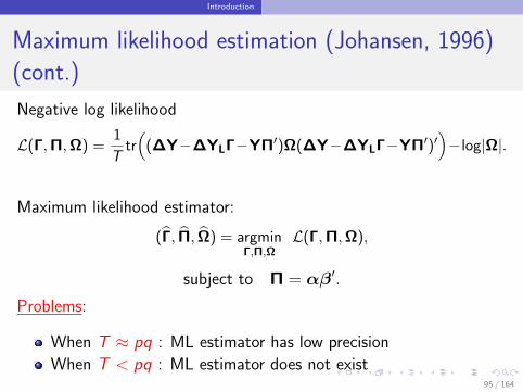
Negative log likelihood
L(Γ,Π,Ω) =1
Ttr((∆Y−∆YLΓ−YΠ′)Ω(∆Y−∆YLΓ−YΠ′)′
)−log|Ω|.
Maximum likelihood estimator:
(Γ, Π, Ω) = argminΓ,Π,Ω
L(Γ,Π,Ω),
subject to Π = αβ′.
Problems:
When T ≈ pq : ML estimator has low precision
When T < pq : ML estimator does not exist95 / 164

Penalized Estimation
Section 2
Penalized Estimation
96 / 164
Penalized Estimation
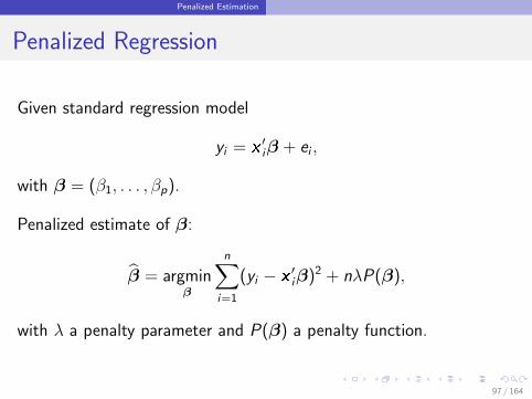
Penalized Regression
Given standard regression model
yi = x′iβ + ei ,
with β = (β1, . . . , βp).
Penalized estimate of β:
β = argminβ
n∑i=1
(yi − x′iβ)2 + nλP(β),
with λ a penalty parameter and P(β) a penalty function.
97 / 164
Penalized Estimation
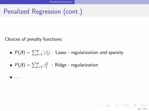
Penalized Regression (cont.)
Choices of penalty functions:
P(β) =∑p
j=1 |βj | : Lasso - regularization and sparsity
P(β) =∑p
j=1 β2j : Ridge - regularization
. . .
98 / 164
Penalized Estimation
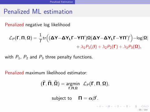
Penalized ML estimation
Penalized negative log likelihood
LP(Γ,Π,Ω) =1
Ttr((∆Y−∆YLΓ−YΠ′)Ω(∆Y−∆YLΓ−YΠ′)′
)−log|Ω|
+ λ1P1(β) + λ2P2(Γ) + λ3P3(Ω),
with P1, P2 and P3 three penalty functions.
Penalized maximum likelihood estimator:
(Γ, Π, Ω) = argminΓ,Π,Ω
LP(Γ,Π,Ω),
subject to Π = αβ′.
99 / 164

Penalized Estimation
Algorithm
Iterative procedure:
1 Solve for Π conditional on Γ,Ω
2 Solve for Γ conditional on Π,Ω
3 Solve for Ω conditional on Γ,Π
100 / 164
Penalized Estimation
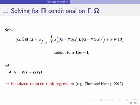
1. Solving for Π conditional on Γ,Ω
Solve
(α, β)|Γ,Ω = argminα,β
1
Ttr((G− Yβα′)Ω(G− Yβα′)′
)+ λ1P1(β).
subject to α′Ωα = Ir
with
G = ∆Y −∆YLΓ
→ Penalized reduced rank regression (e.g. Chen and Huang, 2012)
101 / 164
Penalized Estimation
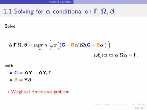
1.1 Solving for α conditional on Γ,Ω,β
Solve
α|Γ,Ω,β = argminα
1
Ttr(
(G− Bα′)Ω(G− Bα′)′)
subject to α′Ωα = Ir ,
with
G = ∆Y −∆YLΓ
B = Yβ
→ Weighted Procrustes problem
102 / 164
Penalized Estimation
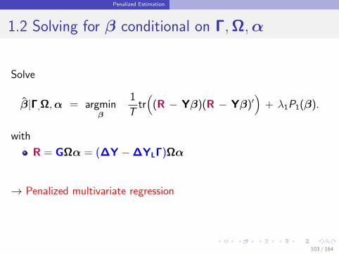
1.2 Solving for β conditional on Γ,Ω,α
Solve
β|Γ,Ω,α = argminβ
1
Ttr(
(R − Yβ)(R − Yβ)′)
+ λ1P1(β).
with
R = GΩα = (∆Y −∆YLΓ)Ωα
→ Penalized multivariate regression
103 / 164

Penalized Estimation
Choice of penalty function
Our choice:
Lasso penalty: P1(β) =∑q
i=1
∑rj=1 |βij |
Other penalty functions are possible:
Adaptive Lasso: P1(β) =∑q
i=1
∑rj=1 wij |βij |
Weights : wij = 1/|βinitialij |
. . .
104 / 164
Penalized Estimation
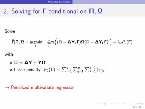
2. Solving for Γ conditional on Π,Ω
Solve
Γ|Π,Ω = argminΓ
1
Ttr((D−∆YLΓ)Ω(D−∆YLΓ)′
)+ λ2P2(Γ).
with
D = ∆Y − YΠ′
Lasso penalty: P2(Γ) =∑q
i=1
∑qj=1
∑p−1k=1 |γijk |
→ Penalized multivariate regression
105 / 164
Penalized Estimation
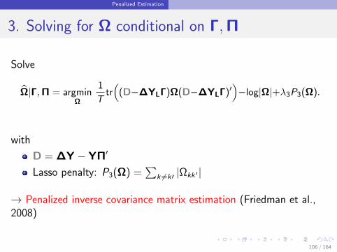
3. Solving for Ω conditional on Γ,Π
Solve
Ω|Γ,Π = argminΩ
1
Ttr((D−∆YLΓ)Ω(D−∆YLΓ)′
)−log|Ω|+λ3P3(Ω).
with
D = ∆Y − YΠ′
Lasso penalty: P3(Ω) =∑
k 6=k′ |Ωkk ′ |
→ Penalized inverse covariance matrix estimation (Friedman et al.,2008)
106 / 164
Penalized Estimation
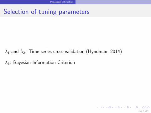
Selection of tuning parameters
λ1 and λ2: Time series cross-validation (Hyndman, 2014)
λ3: Bayesian Information Criterion
107 / 164
Penalized Estimation
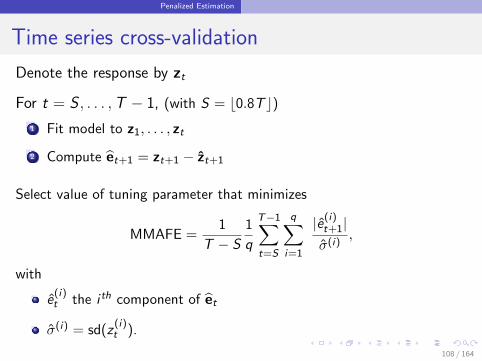
Time series cross-validation
Denote the response by zt
For t = S , . . . ,T − 1, (with S = b0.8T c)1 Fit model to z1, . . . , zt
2 Compute et+1 = zt+1 − zt+1
Select value of tuning parameter that minimizes
MMAFE =1
T − S
1
q
T−1∑t=S
q∑i=1
|e(i)t+1|σ(i)
,
with
e(i)t the i th component of et
σ(i) = sd(z(i)t ).
108 / 164
Penalized Estimation
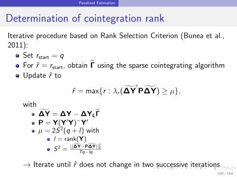
Determination of cointegration rank
Iterative procedure based on Rank Selection Criterion (Bunea et al.,2011):
Set rstart = q
For r = rstart, obtain Γ using the sparse cointegrating algorithm
Update r to
r = maxr : λr (∆Y′P∆Y) ≥ µ,
with∆Y = ∆Y −∆YLΓP = Y(Y′Y)−Y′
µ = 2S2(q + l) withl = rank(Y)
S2 =||∆Y−P∆Y||2F
Tq−lq
→ Iterate until r does not change in two successive iterations109 / 164

Penalized Estimation
Determination of cointegration rank (cont.)
Properties of Rank Selection Criterion :
Consistent estimate of rank(Π)
Low computational cost
110 / 164

Penalized Estimation
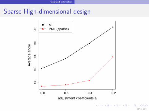
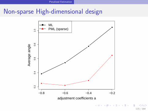
Simulation Study
VECM(1) with dimension q:
∆yt = αβ′yt−1 + Γ1∆yt−1 + et , (t = 1, . . . ,T ),
where et follows Nq(0, Iq).
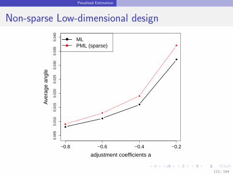
Designs:1 Low-dimensional design: T = 500, q = 4, r = 1
– Sparse cointegrating vector– Non-sparse cointegrating vector
2 High-dimensional design: T = 50, q = 11, r = 1
– Sparse cointegrating vector– Non-sparse cointegrating vector
111 / 164

Penalized Estimation
Sparse Low-dimensional designAverage angle between estimated and true cointegration space
0.00
50.
010
0.01
50.
020
0.02
50.
030
0.03
5
adjustment coefficients a
Ave
rage
ang
le
−0.8 −0.6 −0.4 −0.2
ML PML (sparse)
112 / 164
Penalized Estimation
Non-sparse Low-dimensional design
0.00
50.
010
0.01
50.
020
0.02
50.
030
0.03
50.
040
adjustment coefficients a
Ave
rage
ang
le
−0.8 −0.6 −0.4 −0.2
ML PML (sparse)
113 / 164
Penalized Estimation
Sparse High-dimensional design
0.2
0.4
0.6
0.8
1.0
adjustment coefficients a
Ave
rage
ang
le
−0.8 −0.6 −0.4 −0.2
ML PML (sparse)
114 / 164
Penalized Estimation
Non-sparse High-dimensional design
0.2
0.4
0.6
0.8
1.0
adjustment coefficients a
Ave
rage
ang
le
−0.8 −0.6 −0.4 −0.2
ML PML (sparse)
115 / 164

Forecasting Applications
Section 3
Forecasting Applications
116 / 164
Forecasting Applications
Rolling window forecast with window size S
Estimate the VECM at t = S , . . . ,T − h
∆yt+h =
p−1∑i=1
Γi∆yt+1−i + Πyt ,
for forecast horizon h.
Obtain h-step-ahead multivariate forecast errors
et+h = ∆yt+h − ∆yt+h.
117 / 164
Forecasting Applications
Forecast error measures
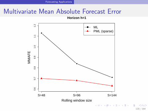
Multivariate Mean Absolute Forecast Error:
MMAFE =1
T − h − S + 1
T−h∑t=S
1
q
q∑i=1
|∆y(i)t+h − ∆y
(i)
t+h|σ(i)
,
where σ(i) is the standard deviation of the i th time series indifferences.
118 / 164
Forecasting Applications
Interest Rate Growth Forecasting
Interest Data: q = 5 monthly US treasury bills
Maturity: 1, 3, 5, 7 and 10 year
Data range: January 1969 - June 2015
Methods: PML (sparse) versus ML
119 / 164
Forecasting Applications
Multivariate Mean Absolute Forecast Error
0.6
0.7
0.8
0.9
1.0
1.1
1.2
Horizon h=1
Rolling window size
MM
AF
E
S=48 S=96 S=144
MLPML (sparse)
120 / 164
Forecasting Applications
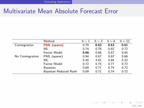
Consumption Growth Forecasting
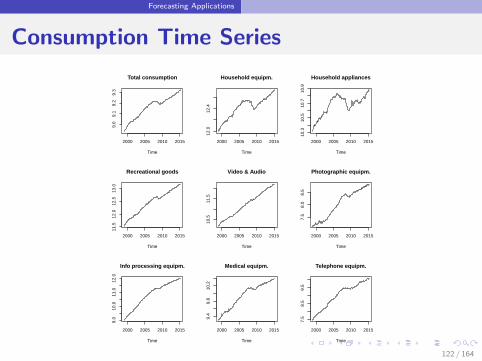
Data: q = 31 monthly consumption time series
Total consumption and industry-specific consumption
Data range: January 1999-April 2015
Forecast: Rolling window of size S = 144
Methods:
Cointegration: PML (sparse), ML, Factor Model
No cointegration: PML (sparse), ML, Factor Model, Bayesian,Bayesian Reduced Rank
121 / 164
Forecasting Applications
Consumption Time Series
Total consumption
Time
2000 2005 2010 2015
9.0
9.1
9.2
9.3
Household equipm.
Time
2000 2005 2010 2015
12.0
12.4
Household appliances
Time
2000 2005 2010 2015
10.3
10.5
10.7
10.9
Recreational goods
Time
2000 2005 2010 2015
11.5
12.0
12.5
13.0
Video & Audio
Time
2000 2005 2010 2015
10.5
11.5
Photographic equipm.
Time
2000 2005 2010 2015
7.5
8.0
8.5
Info processing equipm.
Time
2000 2005 2010 2015
9.0
10.0
11.0
12.0
Medical equipm.
Time
2000 2005 2010 2015
9.4
9.8
10.2
Telephone equipm.
Time
2000 2005 2010 2015
7.5
8.5
9.5
122 / 164
Forecasting Applications
Multivariate Mean Absolute Forecast Error
Method h = 1 h = 3 h = 6 h = 12Cointegration PML (sparse) 0.79 0.62 0.63 0.61
ML 0.74 0.78 0.82 0.72Factor Model 0.66 0.66 0.67 0.65
No Cointegration PML (sparse) 0.94 0.67 0.67 0.66ML 5.40 4.81 4.84 5.22Factor Model 0.72 0.75 0.77 0.72Bayesian 0.69 0.71 0.74 0.72Bayesian Reduced Rank 0.69 0.71 0.74 0.72
123 / 164

Forecasting Applications
References
1 Wilms, I. and Croux, C. (2016), “Forecasting using sparse cointegration,” InternationalJournal of Forecasting, 32(4), 1256-1267.
2 Bunea, F.; She, Y. and Wegkamp, M. (2011), “Optimal selection of reduced rankestimators of high-dimensional matrices,” The Annals of Statistics, 39, 1282-1309.
3 Chen, L. and Huang, J. (2012), “Sparse reduced-rank regression for simultaneousdimension reduction and variable selection,” Journal of the American StatisticalAssociation,107, 1533-1545.
4 Friedman, J., Hastie, T. and Tibshirani, R. (2008), “Sparse inverse covariance estimationwith the graphical lasso,” Biostatistics, 9, 432-441.
5 Johansen (1996), Likelihood-based inference in cointegrated vector autoregressivemodels, Oxford: Oxford University Press.
6 Gelper, S., Wilms, I. and Croux, C. (2016), “Identifying demand effects in a largenetwork of product categories,” Journal of Retailing, 92(1), 25-39.
124 / 164

Part V
Robust Exponential Smoothing
125 / 164

Outline
1 Introduction
2 Exponential Smoothing
3 Robust approach
4 Simulations
5 ROBETS on Real Data
126 / 164

Introduction
Section 1
Introduction
127 / 164
Introduction
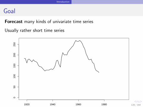
Goal
Forecast many kinds of univariate time series
Usually rather short time series
1920 1940 1960 1980
050
100
150
200
250
Births per 10,000 of 23 year old women, U.S., 1917-1975
128 / 164

Introduction
1980 1985 1990 1995 2000 2005
0e+
004e
+05
8e+
05
Monthly number of unemployed persons in Australia, from February1978 till August 1995
129 / 164
Introduction
1986 1988 1990 1992 1994
2000
6000
1000
0
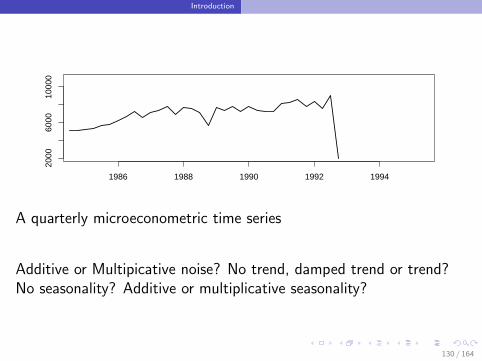
A quarterly microeconometric time series
Additive or Multipicative noise? No trend, damped trend or trend?No seasonality? Additive or multiplicative seasonality?
130 / 164
Introduction
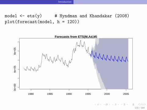
model <- ets(y) # Hyndman and Khandakar (2008)
plot(forecast(model, h = 120))
Forecasts from ETS(M,Ad,M)
1980 1985 1990 1995 2000 2005
0e+
004e
+05
8e+
05
131 / 164
Introduction
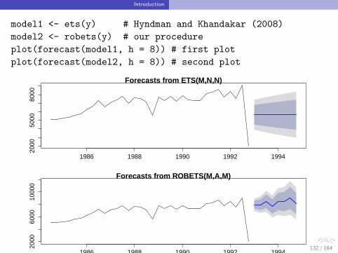
model1 <- ets(y) # Hyndman and Khandakar (2008)
model2 <- robets(y) # our procedure
plot(forecast(model1, h = 8)) # first plot
plot(forecast(model2, h = 8)) # second plot
Forecasts from ETS(M,N,N)
1986 1988 1990 1992 1994
2000
5000
8000
Forecasts from ROBETS(M,A,M)
1986 1988 1990 1992 1994
2000
6000
1000
0
132 / 164

Exponential Smoothing
Section 2
Exponential Smoothing
133 / 164
Exponential Smoothing
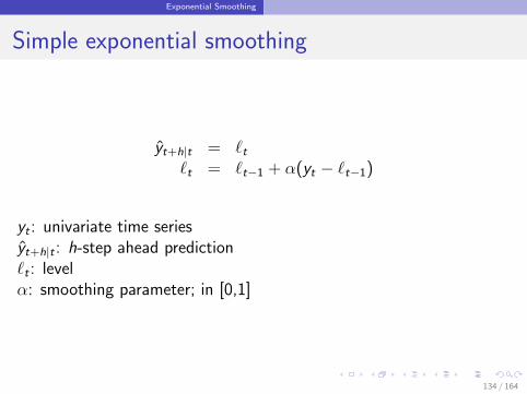
Simple exponential smoothing
yt+h|t = `t`t = `t−1 + α(yt − `t−1)
yt : univariate time seriesyt+h|t : h-step ahead prediction`t : levelα: smoothing parameter; in [0,1]
134 / 164
Exponential Smoothing
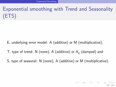
Exponential smoothing with Trend and Seasonality
(ETS)
E, underlying error model: A (additive) or M (multiplicative),
T, type of trend: N (none), A (additive) or Ad (damped) and
S, type of seasonal: N (none), A (additive) or M (multiplicative).
135 / 164
Exponential Smoothing
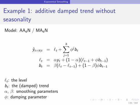
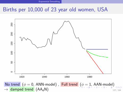
Example 1: additive damped trend without
seasonality
Model: AAdN / MAdN
yt+h|t = `t +h∑
j=1
φjbt
`t = αyt + (1− α)(`t−1 + φbt−1)bt = β(`t − `t−1) + (1− β)φbt−1
`t : the levelbt : the (damped) trendα, β: smoothing parametersφ: damping parameter
136 / 164
Exponential Smoothing
Births per 10,000 of 23 year old women, USA
1920 1940 1960 1980
050
100
150
200
250
y
No trend (φ = 0, ANN-model) , Full trend (φ = 1, AAN-model)→ damped trend (AAdN) 137 / 164
Exponential Smoothing
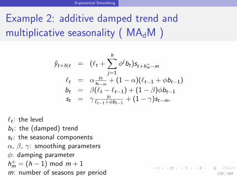
Example 2: additive damped trend and
multiplicative seasonality ( MAdM )
yt+h|t = (`t +h∑
j=1
φjbt)st+h+m−m
`t = α ytst−m
+ (1− α)(`t−1 + φbt−1)
bt = β(`t − `t−1) + (1− β)φbt−1
st = γ yt`t−1+φbt−1
+ (1− γ)st−m.
`t : the levelbt : the (damped) trendst : the seasonal componentsα, β, γ: smoothing parametersφ: damping parameterh+m = (h − 1) mod m + 1
m: number of seasons per period 138 / 164

Exponential Smoothing
Monthly number of unemployed persons in
Australia, from February 1978 till August 1995
1980 1985 1990 1995 2000 2005
0e+
004e
+05
8e+
05
y
No trend (φ = 0, MNM-model) , Full trend (φ = 1, MAM-model)→ damped trend (MAdM)
139 / 164
Exponential Smoothing
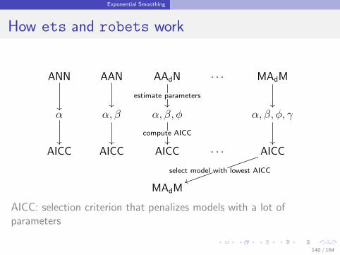
How ets and robets work
ANN
AAN
AAdN
estimate parameters
· · · MAdM
α
α, β
α, β, φ
compute AICC
α, β, φ, γ
AICC AICC AICC · · · AICC
select model with lowest AICCuu
MAdM
AICC: selection criterion that penalizes models with a lot ofparameters
140 / 164

Robust approach
Section 3
Robust approach
141 / 164
Robust approach
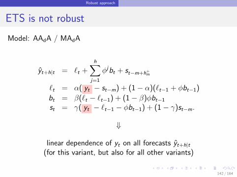
ETS is not robust
Model: AAdA / MAdA
yt+h|t = `t +h∑
j=1
φjbt + st−m+h+m
`t = α( yt − st−m) + (1− α)(`t−1 + φbt−1)
bt = β(`t − `t−1) + (1− β)φbt−1
st = γ( yt − `t−1 − φbt−1) + (1− γ)st−m.
⇓
linear dependence of yt on all forecasts yt+h|t(for this variant, but also for all other variants)
142 / 164
Robust approach
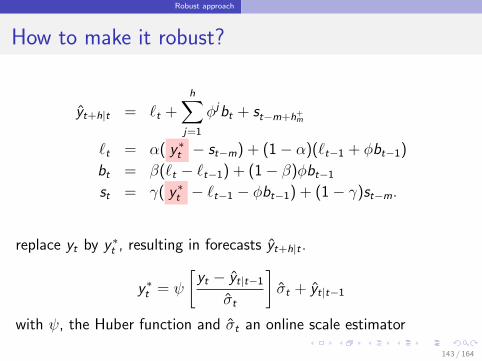
How to make it robust?
yt+h|t = `t +h∑
j=1
φjbt + st−m+h+m
`t = α( y ∗t − st−m) + (1− α)(`t−1 + φbt−1)
bt = β(`t − `t−1) + (1− β)φbt−1
st = γ( y ∗t − `t−1 − φbt−1) + (1− γ)st−m.
replace yt by y ∗t , resulting in forecasts yt+h|t .
y ∗t = ψ
[yt − yt|t−1
σt
]σt + yt|t−1
with ψ, the Huber function and σt an online scale estimator
143 / 164
Robust approach
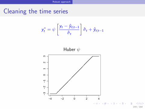
Cleaning the time series
y ∗t = ψ
[yt − yt|t−1
σt
]σt + yt|t−1
Huber ψ
−4 −2 0 2 4
−3
−2
−1
01
23
sapp
ly(x
, psi
.hub
er)
144 / 164
Robust approach
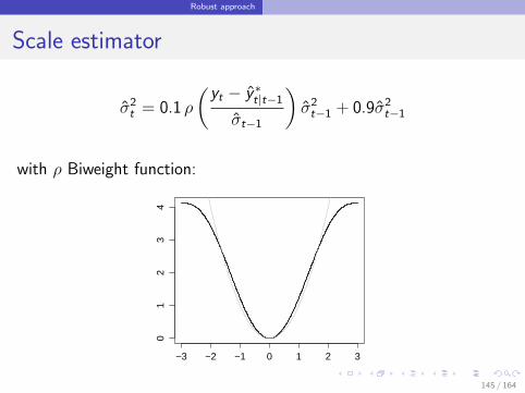
Scale estimator
σ2t = 0.1 ρ
(yt − y ∗t|t−1
σt−1
)σ2t−1 + 0.9σ2
t−1
with ρ Biweight function:
−3 −2 −1 0 1 2 3
01
23
4
sapp
ly(x
, rho
biw
eigh
t)
145 / 164
Robust approach
Estimating parameters
Parameter vector θ: α, β, γ, φ.
`0, b0, s−m+1, . . . , s0 are estimated in a short startup period.
146 / 164
Robust approach
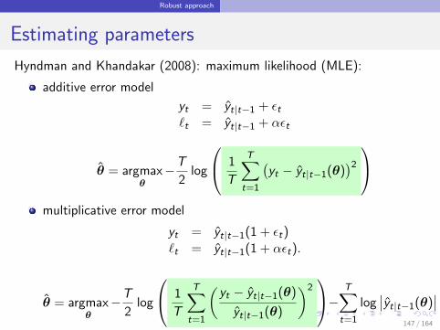
Estimating parameters
Hyndman and Khandakar (2008): maximum likelihood (MLE):
additive error model
yt = yt|t−1 + εt`t = yt|t−1 + αεt
θ = argmaxθ−T
2log
1
T
T∑t=1
(yt − yt|t−1(θ)
)2
multiplicative error model
yt = yt|t−1(1 + εt)`t = yt|t−1(1 + αεt).
θ = argmaxθ−T
2log
1
T
T∑t=1
(yt − yt|t−1(θ)
yt|t−1(θ)
)2− T∑
t=1
log∣∣yt|t−1(θ)
∣∣147 / 164
Robust approach
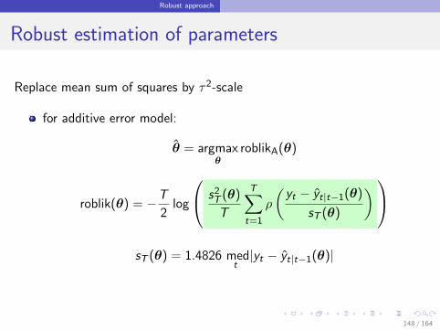
Robust estimation of parameters
Replace mean sum of squares by τ2-scale
for additive error model:
θ = argmaxθ
roblikA(θ)
roblik(θ) = −T
2log
s2T (θ)
T
T∑t=1
ρ
(yt − yt|t−1(θ)
sT (θ)
) sT (θ) = 1.4826 med
t|yt − yt|t−1(θ)|
148 / 164
Robust approach
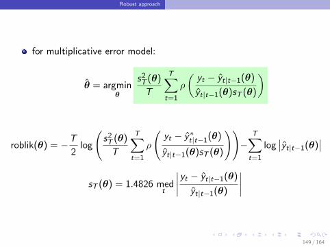
for multiplicative error model:
θ = argminθ
s2T (θ)
T
T∑t=1
ρ
(yt − yt|t−1(θ)
yt|t−1(θ)sT (θ)
)
roblik(θ) = −T
2log
(s2T (θ)
T
T∑t=1
ρ
(yt − y∗t|t−1(θ)
yt|t−1(θ)sT (θ)
))−
T∑t=1
log∣∣yt|t−1(θ)
∣∣sT (θ) = 1.4826 med
t
∣∣∣∣yt − yt|t−1(θ)
yt|t−1(θ)
∣∣∣∣
149 / 164
Robust approach
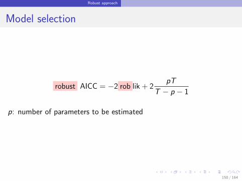
Model selection
robust AICC = −2 rob lik + 2pT
T − p − 1
p: number of parameters to be estimated
150 / 164

Simulations
Section 4
Simulations
151 / 164
Simulations
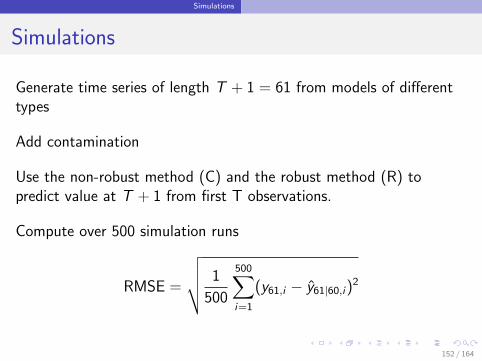
Simulations
Generate time series of length T + 1 = 61 from models of differenttypes
Add contamination
Use the non-robust method (C) and the robust method (R) topredict value at T + 1 from first T observations.
Compute over 500 simulation runs
RMSE =
√√√√ 1
500
500∑i=1
(y61,i − y61|60,i)2
152 / 164
Simulations
t
y
5 10 15
100
200
300
400
500
600
700
t
y
5 10 15
100
200
300
400
500
600
700
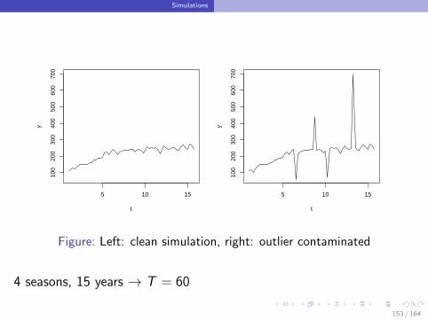
Figure: Left: clean simulation, right: outlier contaminated
4 seasons, 15 years → T = 60
153 / 164
Simulations
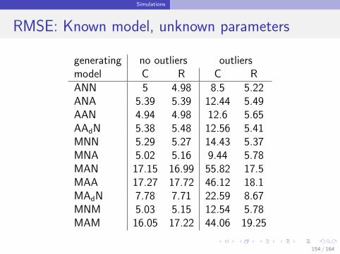
RMSE: Known model, unknown parameters
generating no outliers outliersmodel C R C RANN 5 4.98 8.5 5.22ANA 5.39 5.39 12.44 5.49AAN 4.94 4.98 12.6 5.65AAdN 5.38 5.48 12.56 5.41MNN 5.29 5.27 14.43 5.37MNA 5.02 5.16 9.44 5.78MAN 17.15 16.99 55.82 17.5MAA 17.27 17.72 46.12 18.1MAdN 7.78 7.71 22.59 8.67MNM 5.03 5.15 12.54 5.78MAM 16.05 17.22 44.06 19.25
154 / 164
Simulations
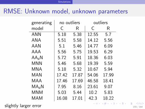
RMSE: Unknown model, unknown parameters
generating no outliers outliersmodel C R C RANN 5.18 5.38 12.55 5.7ANA 5.51 5.58 14.12 5.56AAN 5.1 5.46 14.77 6.09AAA 5.56 5.75 19.53 6.29AAdN 5.72 5.91 18.36 6.03MNN 5.46 5.68 19.39 5.59MNA 5.18 5.32 10.67 5.94MAN 17.42 17.87 54.06 17.99MAA 17.46 17.69 46.58 18.41MAdN 7.95 8.16 23.61 9.07MNM 5.03 5.44 10.2 5.83MAM 16.08 17.01 42.3 18.22
slightly larger error 155 / 164

ROBETS on Real Data
Section 5
ROBETS on Real Data
156 / 164
ROBETS on Real Data
Real data
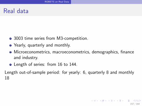
3003 time series from M3-competition.
Yearly, quarterly and monthly.
Microeconometrics, macroeconometrics, demographics, financeand industry.
Length of series: from 16 to 144.
Length out-of-sample period: for yearly: 6, quarterly 8 and monthly18
157 / 164
ROBETS on Real Data
Median Absolute Percentage Error
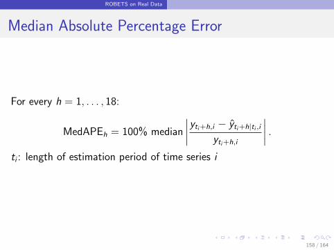
For every h = 1, . . . , 18:
MedAPEh = 100% median
∣∣∣∣yti+h,i − yti+h|ti ,i
yti+h,i
∣∣∣∣ .ti : length of estimation period of time series i
158 / 164
ROBETS on Real Data
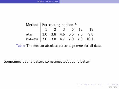
Method Forecasting horizon h1 2 3 6 12 18
ets 3.0 3.8 4.6 6.6 7.0 9.8robets 3.0 3.8 4.7 7.0 7.0 10.1
Table: The median absolute percentage error for all data.
Sometimes ets is better, sometimes robets is better
159 / 164
ROBETS on Real Data
Forecasts from ETS(M,N,N)
1986 1988 1990 1992 1994
2000
5000
8000
Forecasts from ROBETS(M,A,M)
1986 1988 1990 1992 1994
2000
6000
1000
0
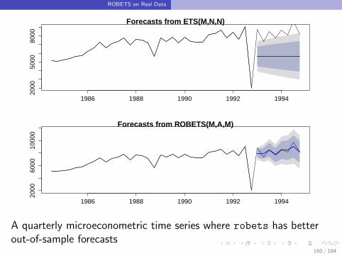
A quarterly microeconometric time series where robets has betterout-of-sample forecasts
160 / 164
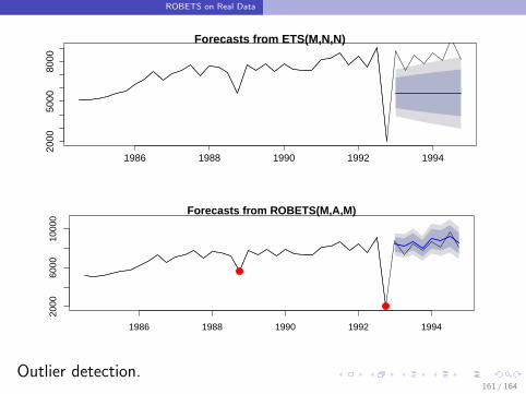
ROBETS on Real Data
Forecasts from ETS(M,N,N)
1986 1988 1990 1992 1994
2000
5000
8000
Forecasts from ROBETS(M,A,M)
1986 1988 1990 1992 1994
2000
6000
1000
0
Outlier detection.161 / 164
ROBETS on Real Data
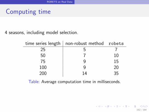
Computing time
4 seasons, including model selection.
time series length non-robust method robets
25 5 750 7 1075 9 15
100 9 20200 14 35
Table: Average computation time in milliseconds.
162 / 164
ROBETS on Real Data
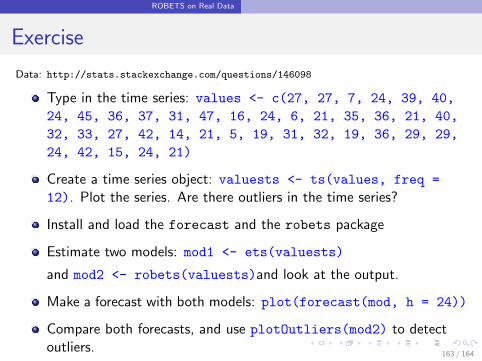
Exercise
Data: http://stats.stackexchange.com/questions/146098
Type in the time series: values <- c(27, 27, 7, 24, 39, 40,
24, 45, 36, 37, 31, 47, 16, 24, 6, 21, 35, 36, 21, 40,
32, 33, 27, 42, 14, 21, 5, 19, 31, 32, 19, 36, 29, 29,
24, 42, 15, 24, 21)
Create a time series object: valuests <- ts(values, freq =
12). Plot the series. Are there outliers in the time series?
Install and load the forecast and the robets package
Estimate two models: mod1 <- ets(valuests)
and mod2 <- robets(valuests)and look at the output.
Make a forecast with both models: plot(forecast(mod, h = 24))
Compare both forecasts, and use plotOutliers(mod2) to detectoutliers.
163 / 164
ROBETS on Real Data
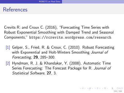
References
Crevits R. and Croux C. (2016), “Forecasting Time Series withRobust Exponential Smoothing with Damped Trend and SeasonalComponents,” https://rcrevits.wordpress.com/research
[1] Gelper, S., Fried, R. & Croux, C. (2010). Robust Forecastingwith Exponential and Holt-Winters Smoothing Journal ofForecasting, 29, 285–300.
[2] Hyndman, R. J. & Khandakar, Y. (2008). Automatic TimeSeries Forecasting: The Forecast Package for R. Journal ofStatistical Software, 27, 3.
164 / 164