T. UzerGeorgia Institute of Technology

Collaboration: C. Chandre (Univ. of Marseille)S. Wiggins (Bristol)

KITP Atto 06 KITP Atto 06 –– September 8, 2006September 8, 2006

TimeTime--frequency analysis of chaotic systemsfrequency analysis of chaotic systems

220

2

2 iii

ii

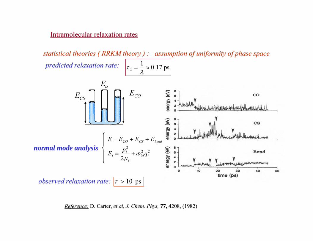
bendCSCO

qpE

EEEE

ωμ

+=

++=normal mode analysisnormal mode analysis

Reference:Reference: D. Carter,D. Carter, et al, J. Chem. Phys,et al, J. Chem. Phys, 77,77, 4208, (1982)4208, (1982)

Intramolecular relaxation ratesIntramolecular relaxation rates

ps 17.01≈=

λτ λ

predicted relaxation rate:predicted relaxation rate:assumption of uniformity of phase space assumption of uniformity of phase space statistical theories ( RRKM theory ) :statistical theories ( RRKM theory ) :

observed relaxation rate:observed relaxation rate: ps 10>τ

CSE COEαE

planar carbonyl sulfide (OCS)planar carbonyl sulfide (OCS)

1R 2R

OC

S

α

m Ii

i ii

H T P P P R VP RVR RAR RR3 3

1 2 1 21

1 2 31

( )( , , , , ( ,, (,) ))α= =

= α + +∑ ∏

quartic polynomialMorsekinetic energy Sorbie-Murrell potential

1

23

2

13

21

32

2

22

1

12213

22

221

1sinsincos

22cos

22 R

PP

R

PP

RRRRPPPPPT

αμ−

αμ−⎟⎟⎠

⎞⎜⎜⎝

⎛ αμ−

μ+

μ+αμ+

μ+

μ= αα

α

( )2)( 0

1)( iii RRiim eDRV −β−−=

( ))~(tanh1)( iiiiI RRRV −γ−=

∑ ∑ ∑ ∑++++=i ji kji lkji

lkjiijklkjiijkjiijii RRRRcRRRcRRcRcRRRP, ,, ,,,

321 1),,(

α−+== cos2 212

22

13 RRRROSR

References:Carter, Brumer, J. Chem. Phys. 77 (1982), 4208Foord, Smith, Whiffen, Mol. Phys. 29 (1975), 1685Bunker, J. Chem. Phys. 37 (1962), 393

>> 3 modes: OC stretch, CS stretch, OCS bend

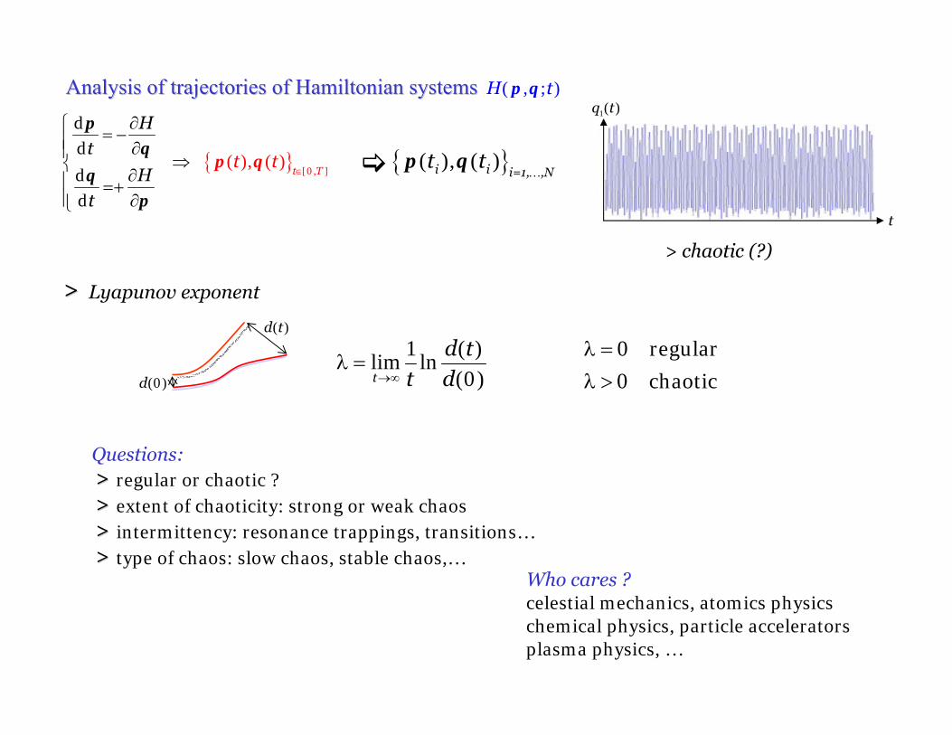
Who cares ?celestial mechanics, atomics physicschemical physics, particle acceleratorsplasma physics, …

Analysis of trajectories of Hamiltonian systemsAnalysis of trajectories of Hamiltonian systems

{ }t T

Ht

Ht

t t[0, ]

dd

( ), ( )dd

∈

∂⎧ = −⎪ ∂⎪ ⇒⎨ ∂⎪ =+⎪ ∂⎩

pq

qp

p q

H t( , ; )p q1( )q t

t

> chaotic (?)

Questions:>> regular or chaotic ?>> extent of chaoticity: strong or weak chaos>> intermittency: resonance trappings, transitions…>> type of chaos: slow chaos, stable chaos,…

{ }i i i=1, ,Nt t( ), ( )p q

…

d(0)

d t( )

t

d tt d1 ( )

lim ln(0)→∞

λ =0 regular

0 chaotic

λ =λ >

>> Lyapunov exponent

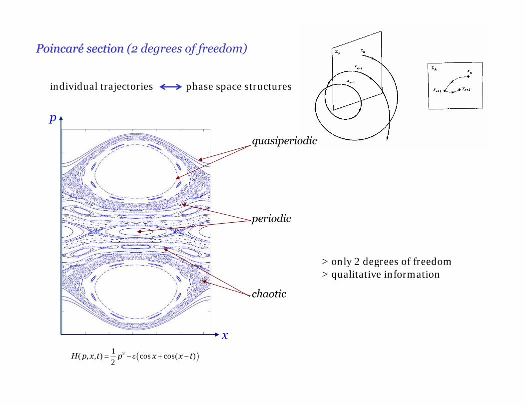
PoincarPoincaréé section section (2 degrees of freedom)

quasiperiodic

periodic

chaotic

p

x

( )H p x t p x x t21( , , ) cos cos( )

2= − ε + −

> only 2 degrees of freedom> qualitative information

individual trajectories phase space structures

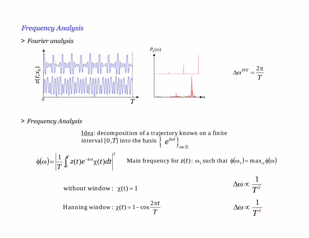
Frequency AnalysisFrequency Analysis

>> Fourier analysis

>> Frequency Analysis

Idea: decomposition of a trajectory known on a finiteinterval [0,T] into the basis

0 T

x(t;

x 0)

ω

)(ωSP

2FFT

Tπ

Δω =

{ }i te ω

ω∈

( )2

0)()(

1∫ χ=ωφ ω−T ti dttetz

T

4

1T

Δω∝T

tt

π−=χ

2cos1)( : windowHanning

1(t) : windowwithout =χ 2

1T

Δω∝

( ) ( )ωφ=ωφω ωmax thatsuch : )(for frequency Main 11tz

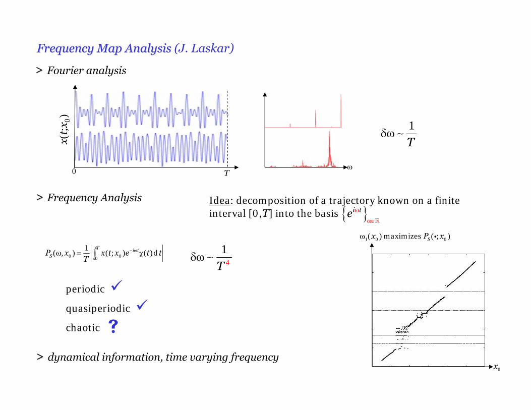
Frequency Map AnalysisFrequency Map Analysis (J. Laskar)

>> Fourier analysis

>> Frequency Analysis Idea: decomposition of a trajectory known on a finiteinterval [0,T] into the basis { }i te ω

ω∈

T i tSP x x t x e t t

T0 00

1( , ) ( ; ) ( )d− ωω = χ∫

Sx P x1 0 0( ) maximizes ( ; )ω i

periodic

quasiperiodic

chaotic

>> dynamical information, time varying frequencyx0

0 T

x(t;

x 0)

ω

T1

δω∼

T 4

1δω∼

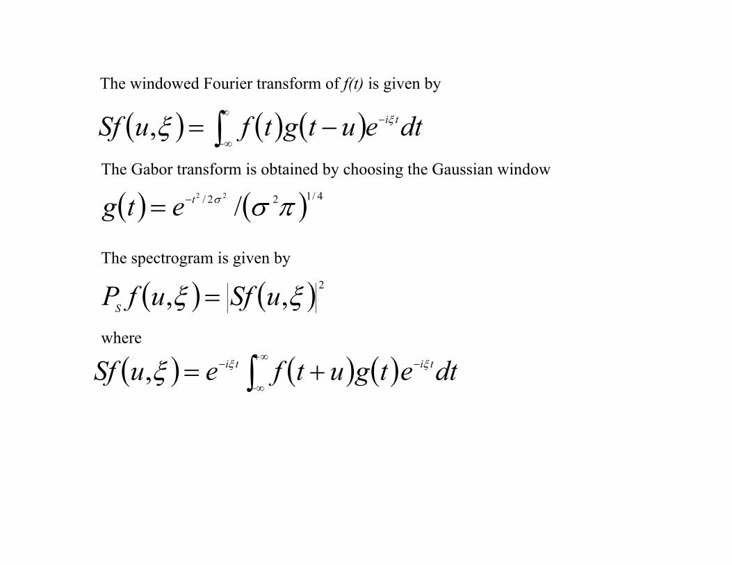
The windowed Fourier transform of f(t) is given by

( ) ( ) ( )∫∞

∞−

−−= dteutgtfuSf tiξξ,The Gabor transform is obtained by choosing the Gaussian window

( ) ( ) 4/122/ /22 πσσtetg −=

The spectrogram is given by

( ) ( ) 2,, ξξ uSfufPS =where

( ) ( ) ( ) dtetgutfeuSf titi ∫∞+

∞−

−− += ξξξ,

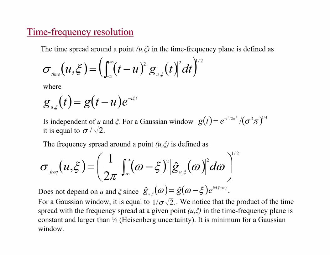
TimeTime--frequency resolutionfrequency resolutionThe time spread around a point (u,ξ) in the time-frequency plane is defined as

( ) ( ) ( )( ) 2/12

,

2, dttgutu utime ∫∞+

∞−−= ξξσ

where

( ) ( ) ti

u eutgtg ξ

ξ

−−=,

Is independent of u and ξ. For a Gaussian windowit is equal to

( ) ( ) 4/122/ /22 πσσtetg −=.2/σ

The frequency spread around a point (u,ξ) is defined as

( ) ( ) ( )2/1

2

,

2 ˆ21, ⎟

⎠⎞

⎜⎝⎛ −= ∫

∞+

∞−ωωξω

πξσ ξ dgu ufreq

Does not depend on u and ξ since ( ) ( ) ( ) .ˆˆ ,

ωξ

ξ ξωω −−= iu

u eggFor a Gaussian window, it is equal to . We notice that the product of the timespread with the frequency spread at a given point (u,ξ) in the time-frequency plane is constant and larger than ½ (Heisenberg uncertainty). It is minimum for a Gaussianwindow.

.2/1 σ

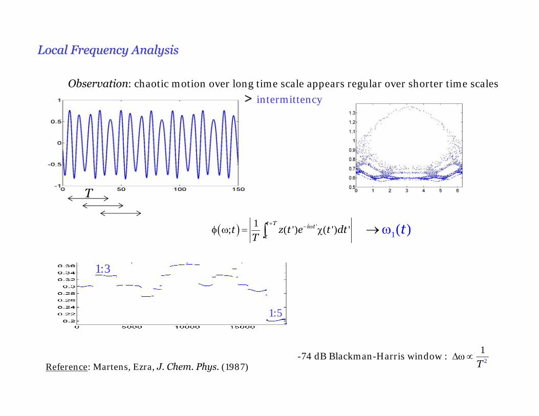
Local Frequency AnalysisLocal Frequency Analysis

Reference: Martens, Ezra, J. Chem. Phys. (1987)

Observation: chaotic motion over long time scale appears regular over shorter time scales

>> intermittency

1:3

( ) '1; ( ') ( ') '

t T i t

tt z t e t dt

T

+ − ωφ ω = χ∫ 1( )t→ω

T

2

1-74 dB Blackman-Harris window :

TΔω∝

1:5

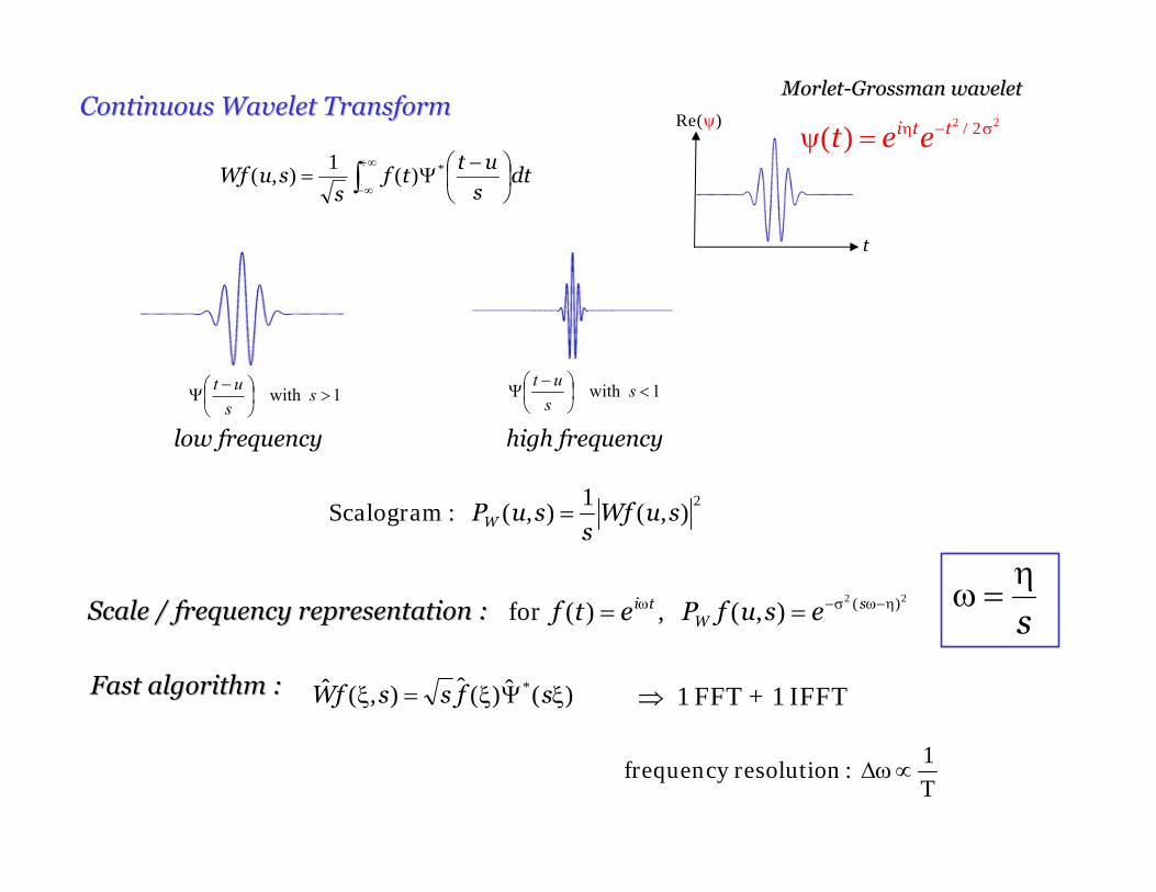
Continuous Wavelet TransformContinuous Wavelet Transform

dts

uttf

ssuWf ∫

∞+

∞−⎟⎠⎞

⎜⎝⎛ −

Ψ= *)(1

),(

Re( )ψ

t

i t tt e e2 2/2( ) η − σψ =

1 with <⎟⎠⎞

⎜⎝⎛ −

Ψ ss

ut1 with >⎟

⎠⎞

⎜⎝⎛ −

Ψ ss

ut

2),(

1),( :Scalogram suWf

ssuPW =

ScaleScale / / frequency representationfrequency representation ::22 )(),( ,)(for η−ωσ−ω == s

Wti esufPetf s

η=ω

Fast algorithmFast algorithm :: )(ˆ)(ˆ),(ˆ * ξΨξ=ξ sfssfW ⇒ 1 FFT + 1 IFFT

T1

: resolution frequency ∝ωΔ

low frequency high frequency

MorletMorlet--Grossman waveletGrossman wavelet

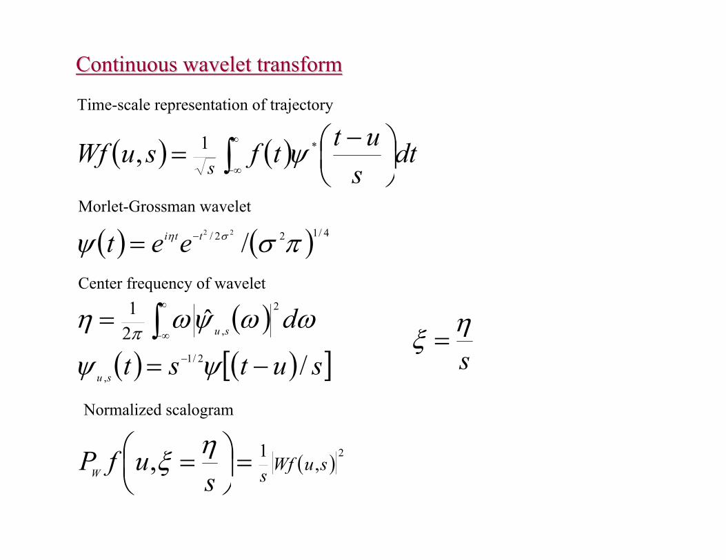
Continuous wavelet transformContinuous wavelet transform

Time-scale representation of trajectory

( ) ( )∫∞

∞−⎟⎠⎞

⎜⎝⎛ −= dt

suttfsuWf s

*1, ψ

Morlet-Grossman wavelet

( ) ( ) 4/122/ /22 πσψ ση tti eet −=Center frequency of wavelet

( )( ) ( )[ ]sutst

d

su

su

/

ˆ2/1

,

2

,21

−=

=−

∞

∞−∫ψψ

ωωψωη π

sηξ =

Normalized scalogram

( )2

,1, suWfss

ufPW =⎟⎠⎞

⎜⎝⎛ =ηξ

freq

uen

cy

time

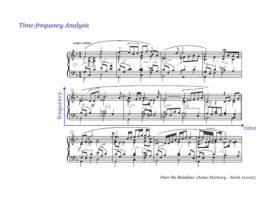
TimeTime--frequency Analysisfrequency Analysis

Over the Rainbow (Arlen/Harburg – Keith Jarrett)

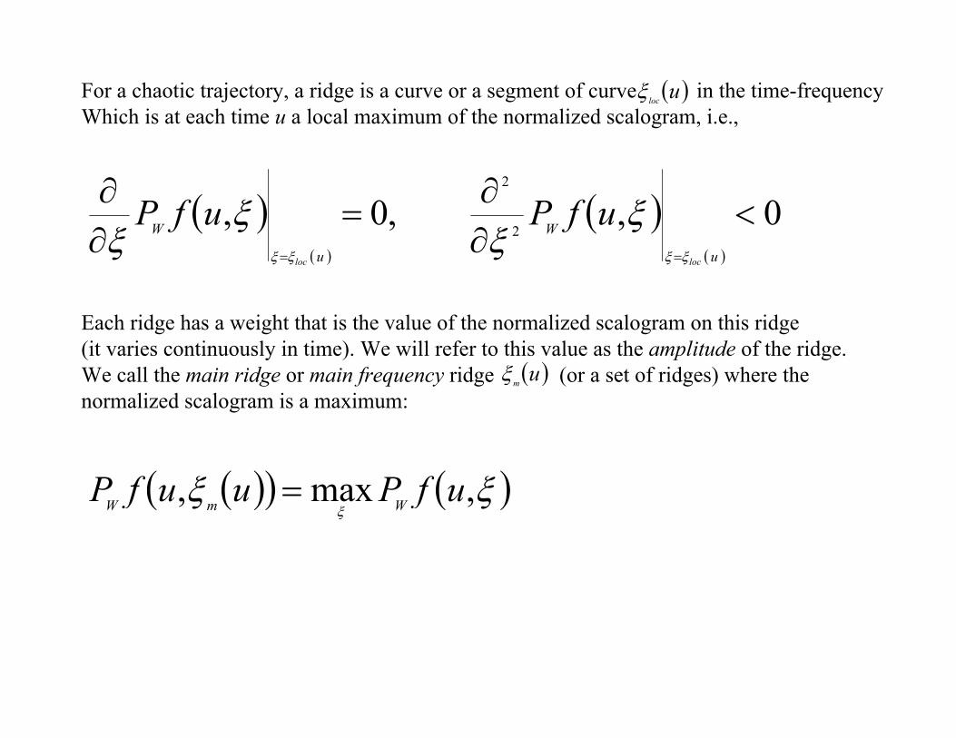
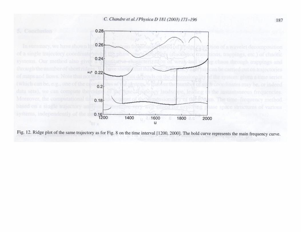
For a chaotic trajectory, a ridge is a curve or a segment of curve in the time-frequencyWhich is at each time u a local maximum of the normalized scalogram, i.e.,

Each ridge has a weight that is the value of the normalized scalogram on this ridge(it varies continuously in time). We will refer to this value as the amplitude of the ridge.We call the main ridge or main frequency ridge (or a set of ridges) where thenormalized scalogram is a maximum:

( )( )

( )( )

0,,0,2

2

<∂∂=

∂∂

== u

W

u

W

locloc

ufPufPξξξξ

ξξ

ξξ

( )ulocξ

( )umξ

( )( ) ( )ξξξ

,max, ufPuufP WmW =

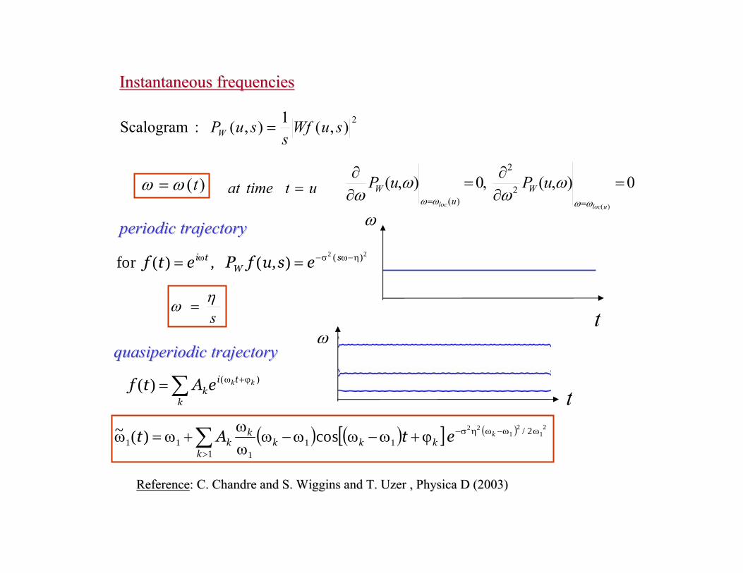
Instantaneous frequenciesInstantaneous frequencies

ReferenceReference: : C. Chandre and S. Wiggins and T. UzerC. Chandre and S. Wiggins and T. Uzer , , Physica DPhysica D (2003)(2003)

∑ ϕ+ω=k

tik

kkeAtf )()(

( ) ( )[ ] ( )∑>

ωω−ωησ−ϕ+ω−ωω−ωωω

+ω=ω1

2/11

111

21

21

22

cos)(~k

kkkk

kketAt

ω

ωt

t

22 )(),( ,)(for η−ωσ−ω == sW

ti esufPetf

2),(1),( :Scalogram suWfs

suPW =

0),( ,0),()(

2

2

)(

=∂∂

=∂∂

== ulocloc

uPuP Wu

Wωωωω

ωω

ωω)( tωω = uttimeat =

periodic trajectoryperiodic trajectory

quasiperiodic trajectoryquasiperiodic trajectory

sηω =

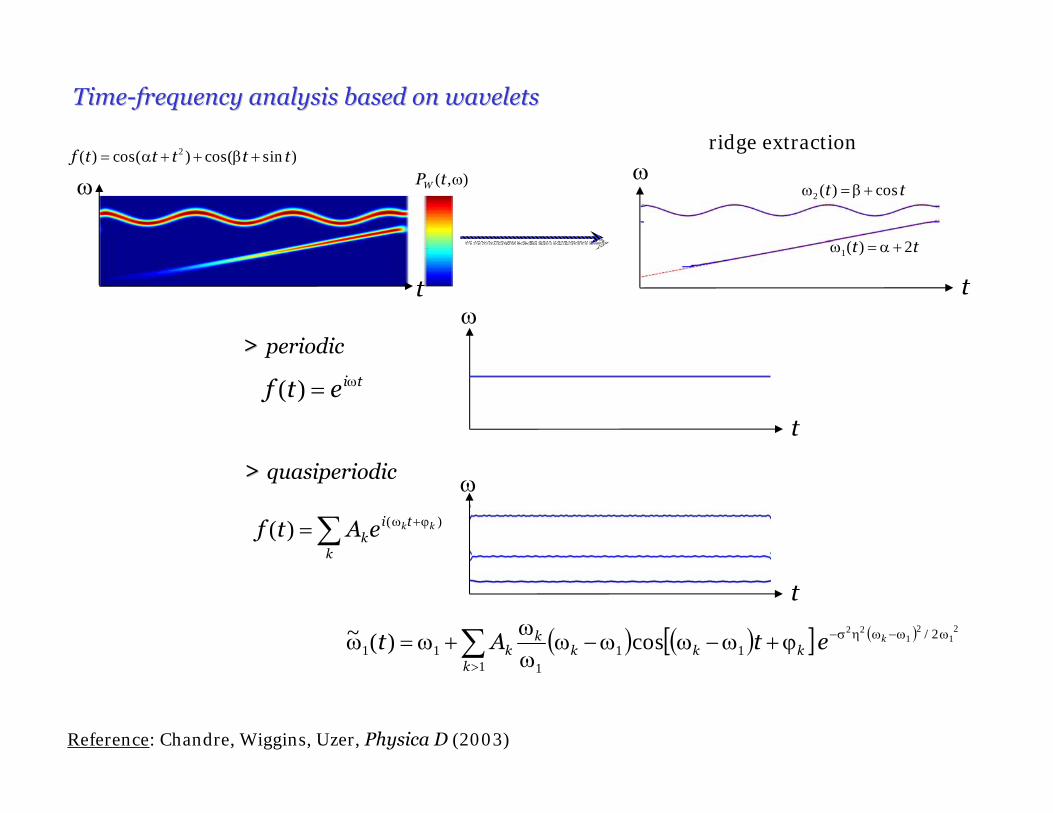
TimeTime--frequency analysis based on waveletsfrequency analysis based on wavelets

t

ωf t t t t t2( ) cos( ) cos( sin )= α + + β +

ω

t

>> periodic

>> quasiperiodic

ω

t

ω

t

),( ωtPW

tt 2)(1 +α=ω

tt cos)(2 +β=ω

Reference: Chandre, Wiggins, Uzer, Physica D (2003)

ridge extraction

∑ ϕ+ω=k

tik

kkeAtf )()(

( ) ( )[ ] ( )∑>

ωω−ωησ−ϕ+ω−ωω−ωωω

+ω=ω1

2/11

111

21

21

22

cos)(~k

kkkk

kketAt

tietf ω=)(

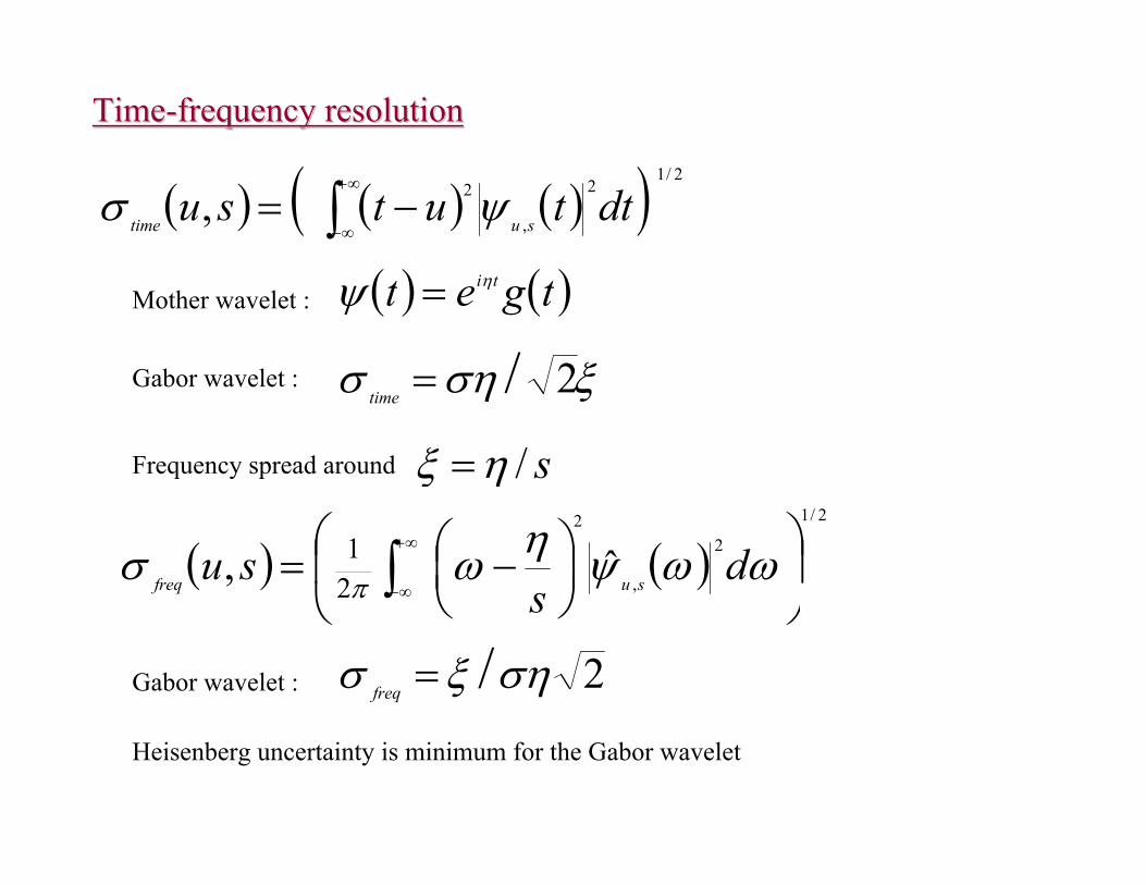
TimeTime--frequency resolutionfrequency resolution

( ) ( ) ( )( ) 2/12

,

2, dttutsu sutime ∫∞+

∞−−= ψσ

( ) ( )2/1

2

,

2

ˆ, 21 ⎟

⎠

⎞⎜⎝

⎛⎟⎠⎞

⎜⎝⎛ −= ∫

∞+

∞−ωωψηωσ π d

ssu sufreq

Mother wavelet : ( ) ( )tget tiηψ =

Gabor wavelet : ξσησ 2/=time

Frequency spread around s/ηξ =

Gabor wavelet : 2/σηξσ =freq

Heisenberg uncertainty is minimum for the Gabor wavelet

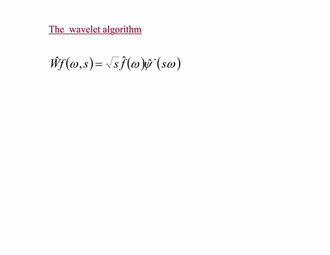
The wavelet algorithmThe wavelet algorithm

( ) ( ) ( )ωψωω sfssfW *ˆˆ,ˆ =

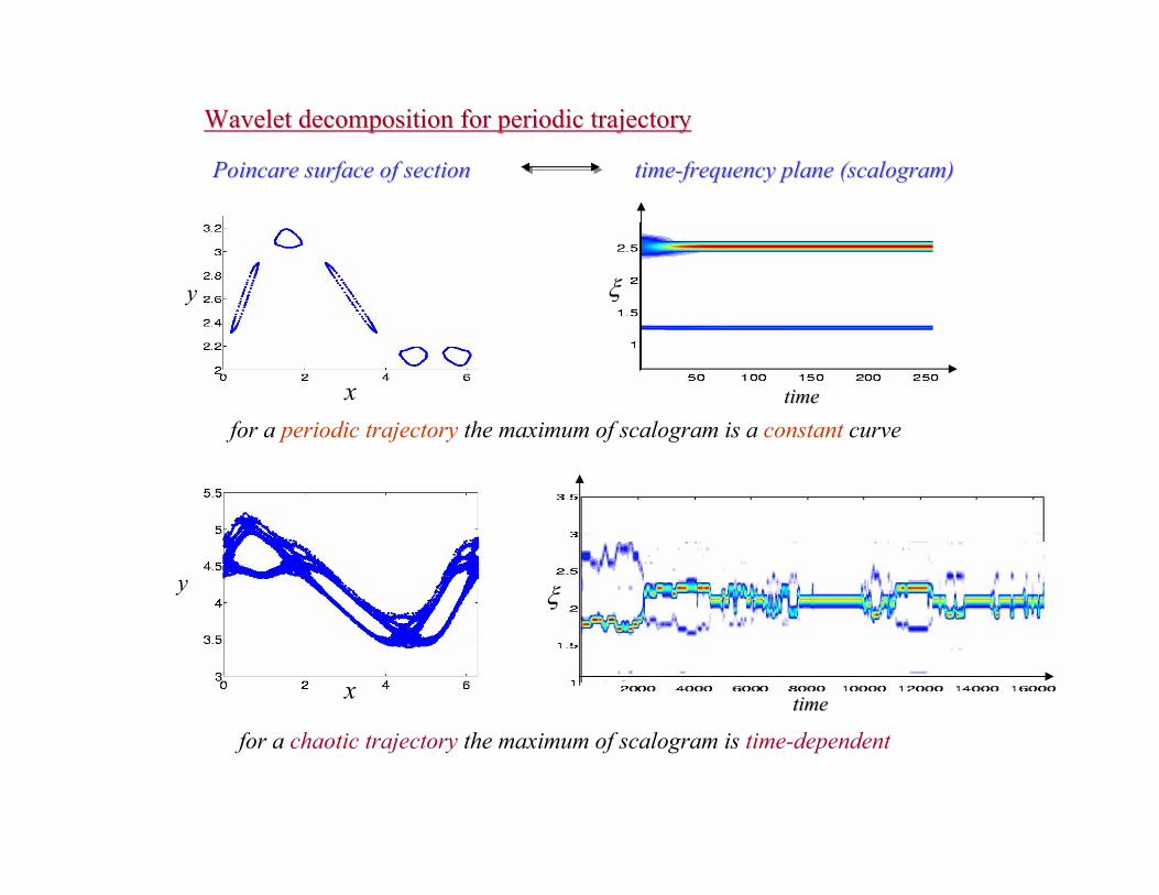
Wavelet decomposition for periodic trajectoryWavelet decomposition for periodic trajectory

Poincare surface of sectionPoincare surface of section timetime--frequency plane (scalogram)frequency plane (scalogram)

timetimex

y

for a periodic trajectory the maximum of scalogram is a constant curve

timetimex

y ξ

ξ

for a chaotic trajectory the maximum of scalogram is time-dependent

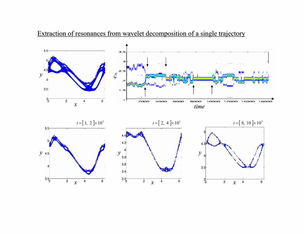
Extraction of resonances from wavelet decomposition of a single Extraction of resonances from wavelet decomposition of a single trajectorytrajectory

xx

xx xxxx

yy yy yy

yy

timetime

ξ

[ ] 310 10 ,8 ×=t[ ] 310 4 ,2 ×=t[ ] 310 2 ,1 ×=t

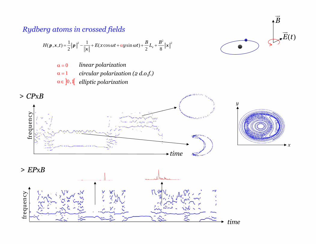
Rydberg atoms in crossed fieldsRydberg atoms in crossed fieldsE t( )

B

z

B BH t E x ωt y ωt L

22 21 1

( , , ) ( cos sin )2 2 8

p x p xx

= − +α+ + +

] [

0

1

0,1

α =α =

α∈

linear polarization

circular polarization (2 d.o.f.)

elliptic polarization

time

freq

uen

cy

x

y

freq

uen

cy

time

>> CPCPxxBB

>> EPEPxxBB

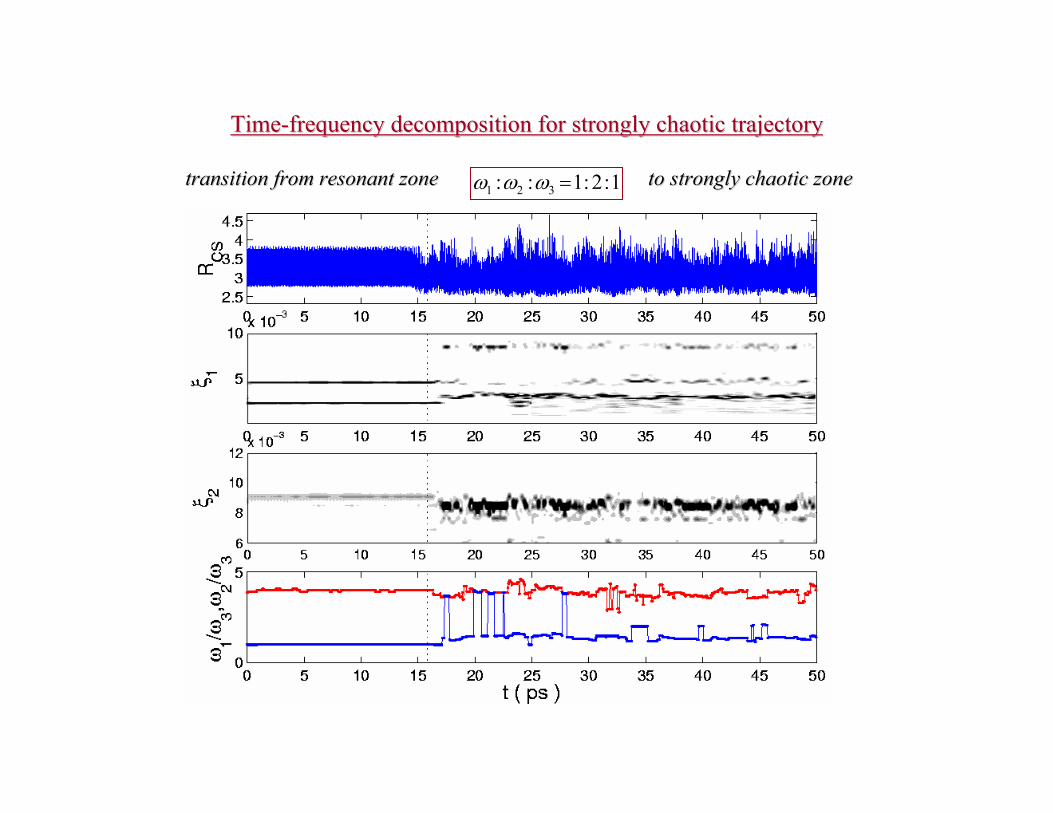
TimeTime--frequency decomposition for strongly chaotic trajectoryfrequency decomposition for strongly chaotic trajectory

transition from resonant zonetransition from resonant zone 1:2:1:: 321 =ωωω to strongly chaotic zoneto strongly chaotic zone

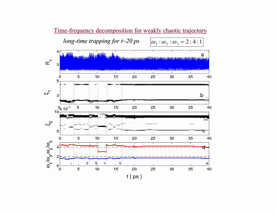
TimeTime--frequency decomposition for weakly chaotic trajectoryfrequency decomposition for weakly chaotic trajectory

1:4:2:: 321 =ωωωlonglong--time trapping for t~20 pstime trapping for t~20 ps

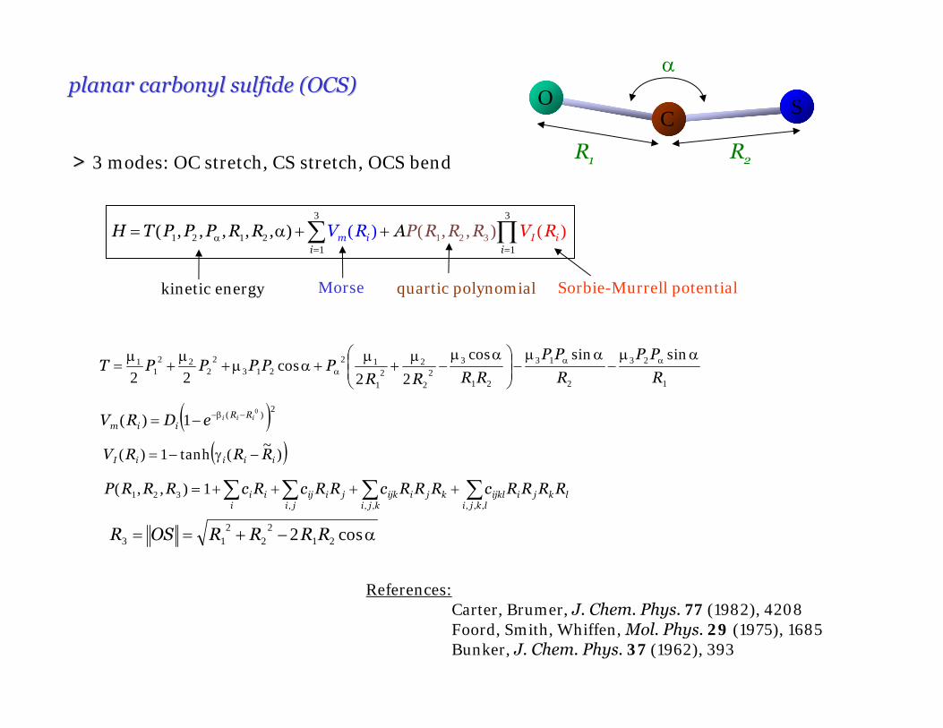
planar carbonyl sulfide (OCS)planar carbonyl sulfide (OCS)

1R 2R

OC

S

α

m Ii

i ii

H T P P P R VP RVR RAR RR3 3

1 2 1 21

1 2 31

( )( , , , , ( ,, (,) ))α= =

= α + +∑ ∏

quartic polynomialMorsekinetic energy Sorbie-Murrell potential

1

23

2

13

21

32

2

22

1

12213

22

221

1sinsincos

22cos

22 R

PP

R

PP

RRRRPPPPPT

αμ−

αμ−⎟⎟⎠

⎞⎜⎜⎝

⎛ αμ−

μ+

μ+αμ+

μ+

μ= αα

α

( )2)( 0

1)( iii RRiim eDRV −β−−=

( ))~(tanh1)( iiiiI RRRV −γ−=

∑ ∑ ∑ ∑++++=i ji kji lkji

lkjiijklkjiijkjiijii RRRRcRRRcRRcRcRRRP, ,, ,,,

321 1),,(

α−+== cos2 212

22

13 RRRROSR

References:Carter, Brumer, J. Chem. Phys. 77 (1982), 4208Foord, Smith, Whiffen, Mol. Phys. 29 (1975), 1685Bunker, J. Chem. Phys. 37 (1962), 393

>> 3 modes: OC stretch, CS stretch, OCS bend

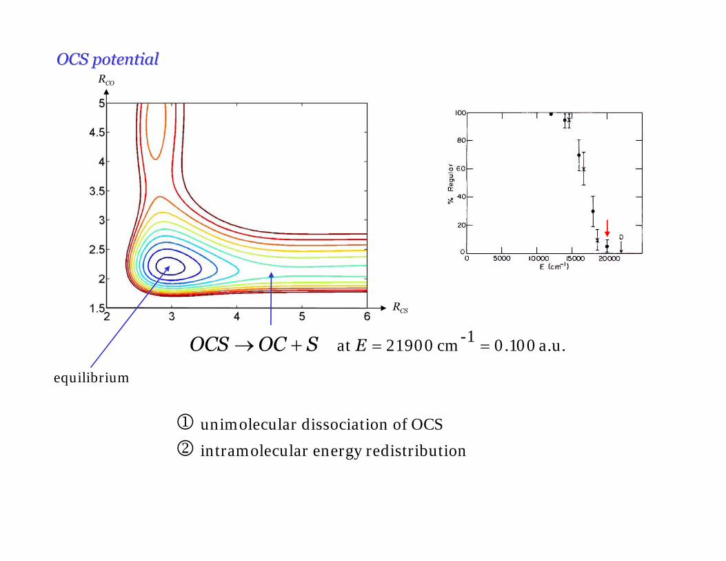
a.u.100.0-1cm 90021 at ==+→ ESOCOCS

COR

CSR

1 unimolecular dissociation of OCS

2 intramolecular energy redistribution

OCS potentialOCS potential

equilibrium

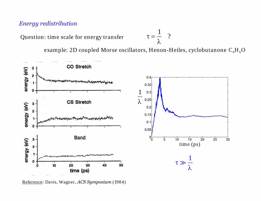
Energy redistributionEnergy redistribution

Question: time scale for energy transfer

example: 2D coupled Morse oscillators, Henon-Heiles, cyclobutanone

1 ?τ =

λOHC 64

1τ

λ

1λ

time (ps)

Reference: Davis, Wagner, ACS Symposium (1984)

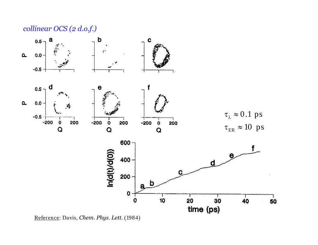
collinear OCS (2 d.o.f.)collinear OCS (2 d.o.f.)

Reference: Davis, Chem. Phys. Lett. (1984)

ps 10

ps 1.0

ER ≈τ

≈τλ

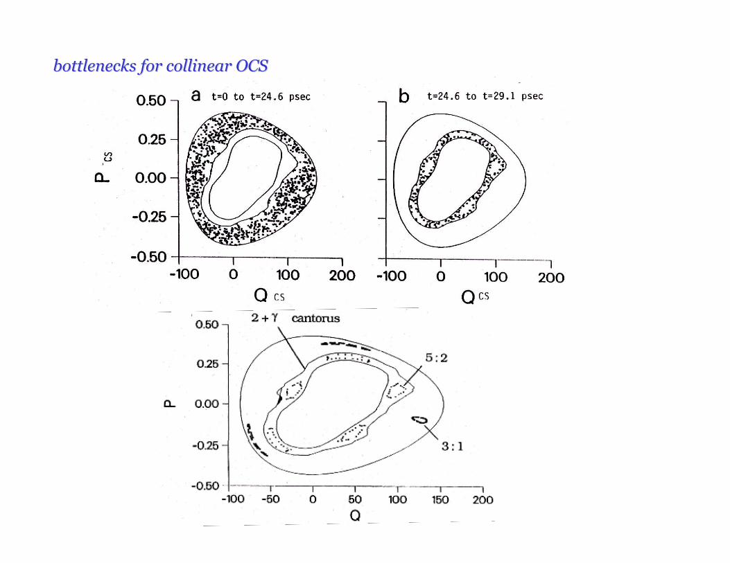
bottlenecks for collinear OCSbottlenecks for collinear OCS

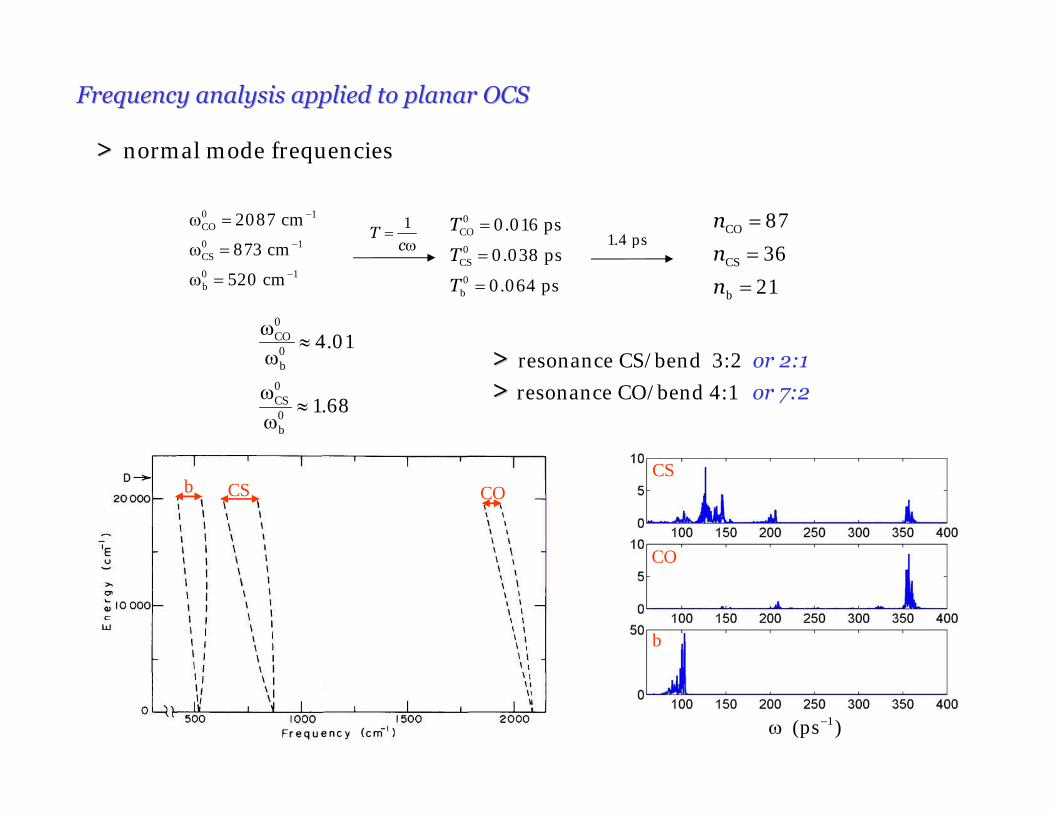
Frequency analysis applied to planar OCSFrequency analysis applied to planar OCS

>> normal mode frequencies

0 1CO

0 1CS

0 1b

2087 cm

873 cm

520 cm

−

−

−

ω =

ω =

ω =

1T

c=

ω

0CO

0CS

0b

0.016 ps

0.038 ps

0.064 ps

T

T

T

=

=

=

CO

CS

b

87

36

21

n

n

n

=

=

=

1.4 ps

>> resonance CS/bend 3:2 or 2:1

>> resonance CO/bend 4:1 or 7:2

0CO0b

0CS0b

4.01

1.68

ω≈

ω

ω≈

ω

COCSb

CO

CS

b

1 (ps )−ω

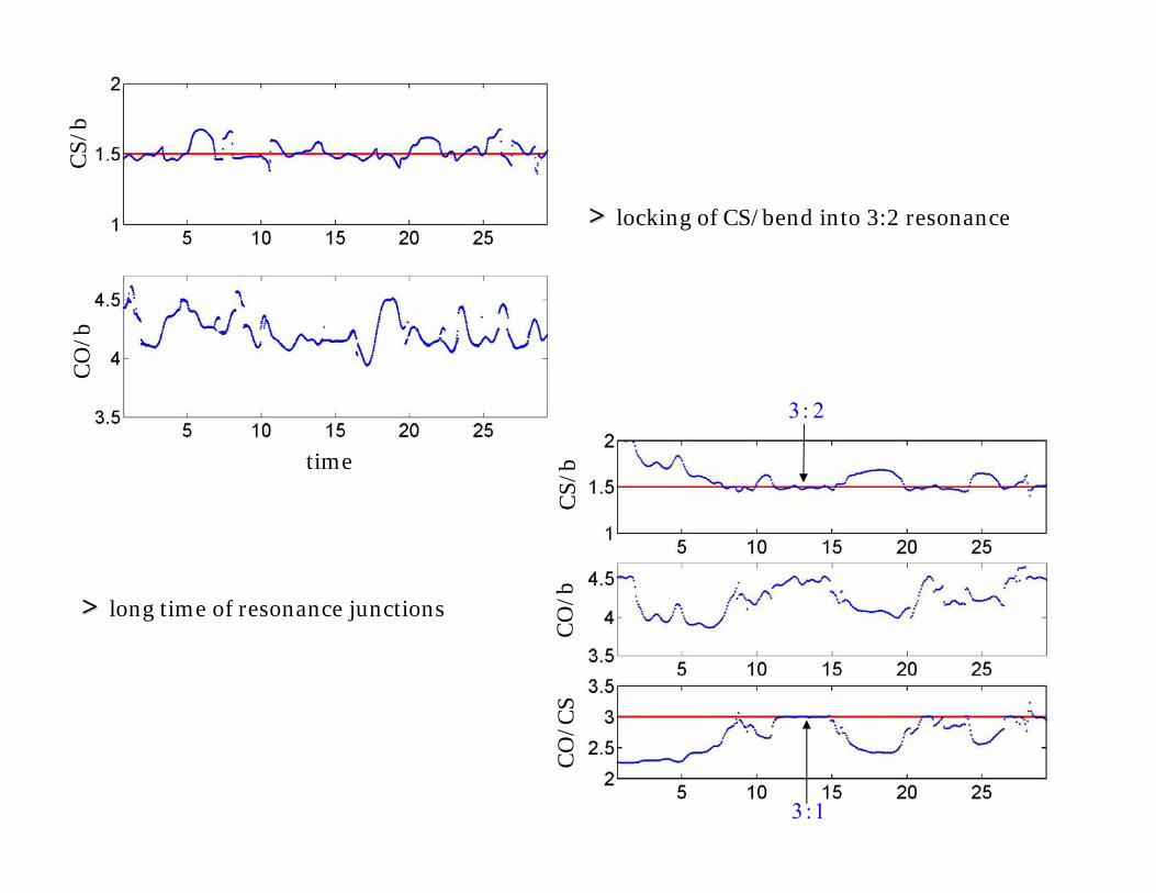
>> locking of CS/bend into 3:2 resonance

>> long time of resonance junctions

3: 2

3:1

CS/

bC

O/b

time

CS/

bC

O/b

CO

/CS

O

CS

R1R1R2R2

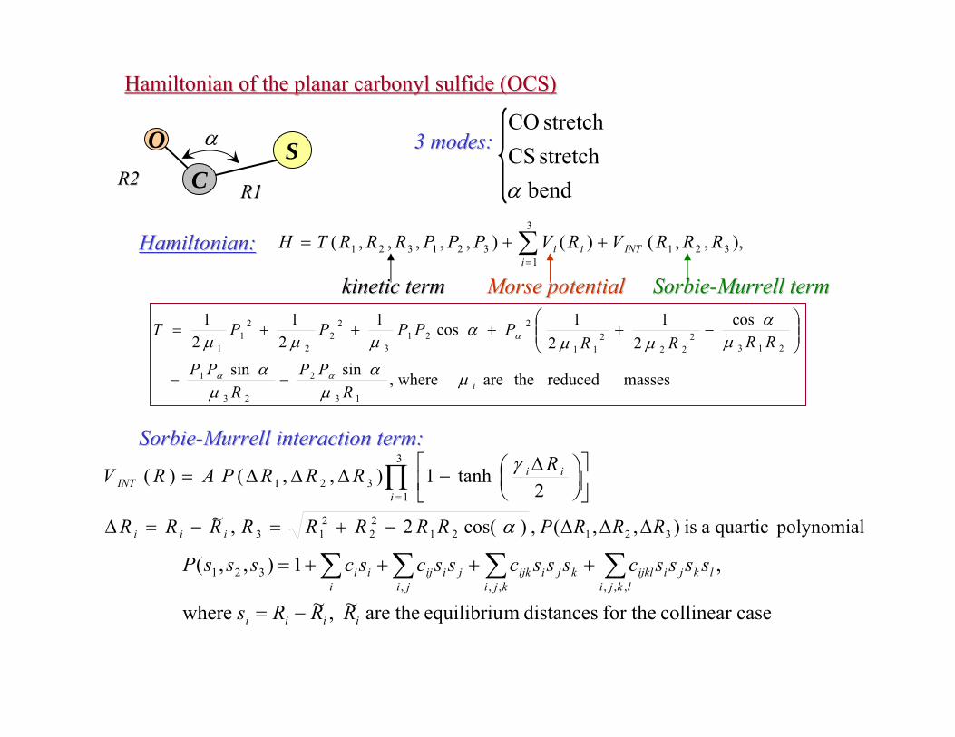
),,,()(),,,,,( 321

3

1321321 RRRVRVPPPRRRTH INTi

ii ++= ∑

=

)cos(2 ,~2

tanh1),,( )(

2122

213

3

1321

α

γ

RRRRRRRR

RRRRPARV

iii

i

iiINT

−+=−=Δ

⎥⎦

⎤⎢⎣

⎡⎟⎠⎞

⎜⎝⎛ Δ

−ΔΔΔ= ∏=

polynomial quartica is )Δ,Δ,(Δ , 321 RRRP

Hamiltonian of the planar carbonyl sulfide (OCS)Hamiltonian of the planar carbonyl sulfide (OCS)

masses reduced theare where,sinsin

cos2

12

1cos12

12

1

13

2

23

1

2132

222

11

221

3

22

2

21

1

iRPP

RPP

RRRRPPPPPT

μμ

αμ

α

μα

μμα

μμμ

αα

α

−−

⎟⎟⎠

⎞⎜⎜⎝

⎛−++++=

Hamiltonian:Hamiltonian:

bend stretch CS stretch CO

α

3 modes:3 modes:α

SorbieSorbie--Murrell interaction term:Murrell interaction term:

SorbieSorbie--Murrell termMurrell termMorse potentialMorse potentialkinetic termkinetic term

casecollinear for the distances mequilibriu theare ~ ,~ where

,1),,(,,,,,,

321

iiii

lkjilkjiijkl

kjikjiijk

jijiij

iii

RRRs

sssscssscsscscsssP

−=

++++= ∑∑∑∑

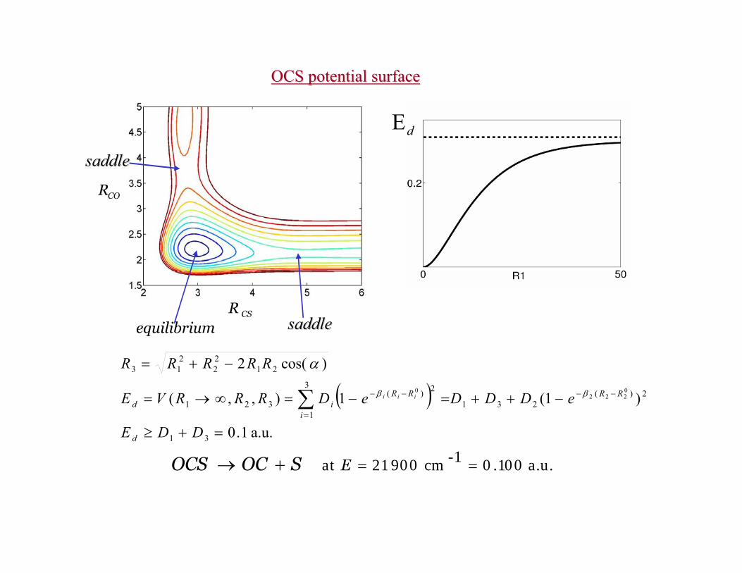
OCS potential surface OCS potential surface

a.u.100.0-1cm 90021 at ==+→ ESOCOCS

equilibriumCSR

COR

( )a.u. 1.0

)1(1),,(

)cos(2

31

2)(231

3

1

2)(321

2122

213

0222

0

=+≥

−++=−=∞→=

−+=

−−

=

−−∑DDE

eDDDeDRRRVE

RRRRR

d

RR

i

RRid

iii ββ

α

dE

saddlesaddle

saddlesaddle

ReferenceReference: : C. C. Martens, C. C. Martens, et al, Chem. Phys. Lett.,et al, Chem. Phys. Lett.,142, 142, 519, (1987) 519, (1987)

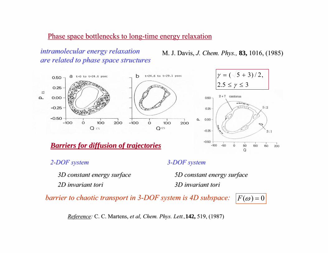
Phase space bottlenecks to longPhase space bottlenecks to long--time energy relaxationtime energy relaxation

M. J. Davis, M. J. Davis, J. Chem. Phys.,J. Chem. Phys., 83,83, 1016, (1985)1016, (1985)

32.5 ,2/)35(

≤≤+=

γγ

Barriers for diffusion of trajectoriesBarriers for diffusion of trajectories

intramolecular energy relaxation intramolecular energy relaxation are related to phase space structuresare related to phase space structures

33--DOF systemDOF system

3D constant energy surface3D constant energy surface2D invariant tori 2D invariant tori 3D invariant tori3D invariant tori

5D constant energy surface5D constant energy surface

22--DOF systemDOF system

barrier to chaotic transport in 3barrier to chaotic transport in 3--DOF system is 4D subspace:DOF system is 4D subspace: 0)( =ωF

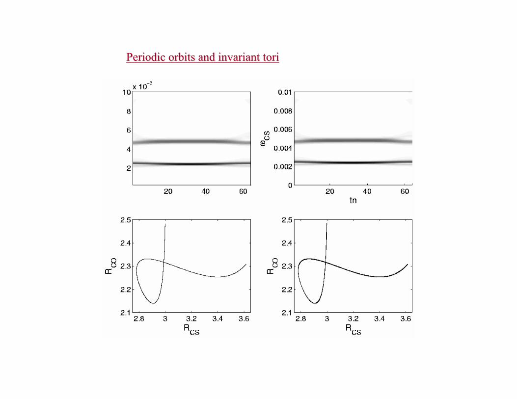
Periodic orbits and invariant toriPeriodic orbits and invariant tori

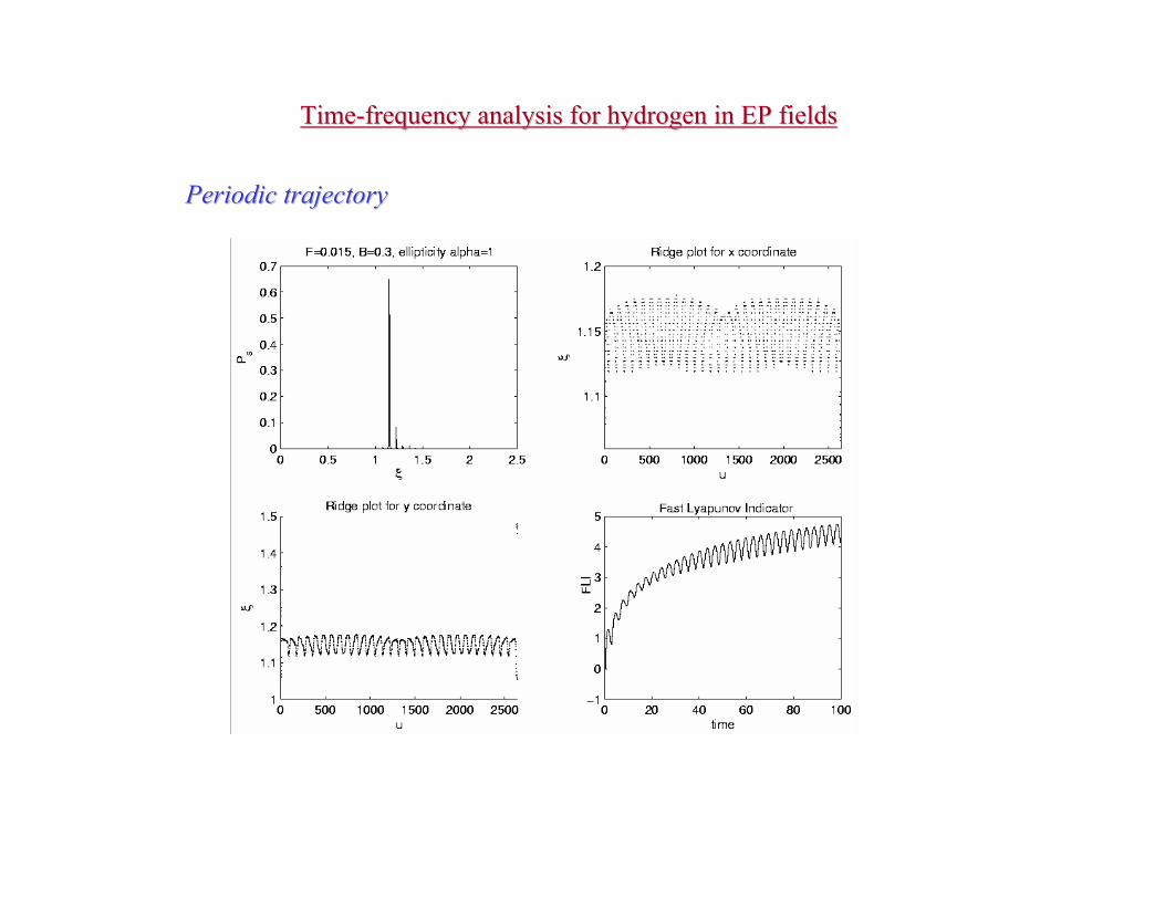
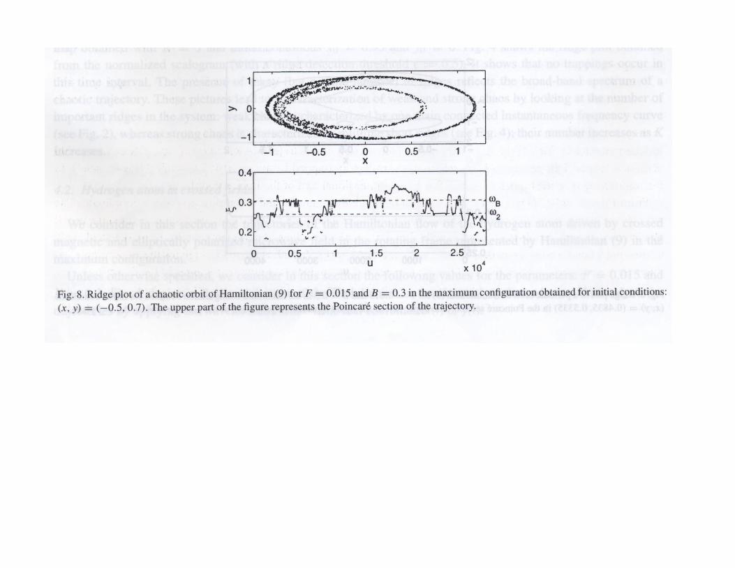
TimeTime--frequency analysis for hydrogen in EP fieldsfrequency analysis for hydrogen in EP fields

Periodic trajectoryPeriodic trajectory

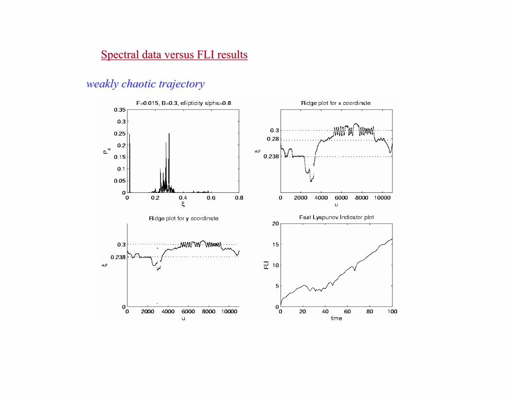
Spectral data versus FLI resultsSpectral data versus FLI results

weakly chaotic trajectoryweakly chaotic trajectory

Spectral data versus FLI resultsSpectral data versus FLI results

strongly chaotic trajectorystrongly chaotic trajectory

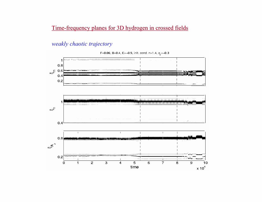
TimeTime--frequency planes for 3D hydrogen in crossed fieldsfrequency planes for 3D hydrogen in crossed fields

weakly chaotic trajectoryweakly chaotic trajectory

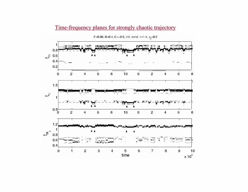
TimeTime--frequency planes for strongly chaotic trajectoryfrequency planes for strongly chaotic trajectory

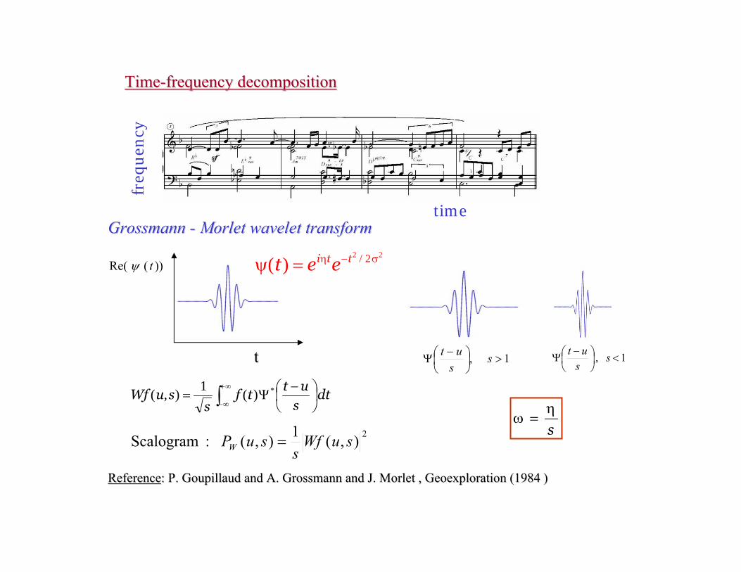
dts

uttf

ssuWf ∫

∞+

∞−⎟⎠⎞

⎜⎝⎛ −

Ψ= *)(1

),(

s

η=ω

2),(1),( :Scalogram suWfs

suPW =

TimeTime--frequency decompositionfrequency decomposition

ReferenceReference: : P. Goupillaud and A. Grossmann and J. MorletP. Goupillaud and A. Grossmann and J. Morlet , , GeoexplorationGeoexploration ((19841984 ))

1 , >⎟⎠⎞

⎜⎝⎛ −

Ψ ss

uttt

))(Re( tψ

freq

uen

cy

timeGrossmann Grossmann -- Morlet wavelet transform Morlet wavelet transform

i t tt e e2 2/2( ) η − σψ =

1 , <⎟⎠⎞

⎜⎝⎛ −

Ψ ss

ut