TI89 and Voyage 200 Student Support Services Presented by Andy Williamson and Amanda Griffin.
84
TI89 and Voyage 200 Student Support Services Presented by Andy Williamson and Amanda Griffin
-
Upload
felix-west -
Category
Documents
-
view
219 -
download
3
Transcript of TI89 and Voyage 200 Student Support Services Presented by Andy Williamson and Amanda Griffin.

TI89 and Voyage 200
Student Support Services
Presented by Andy Williamson and Amanda Griffin
Showing Computations
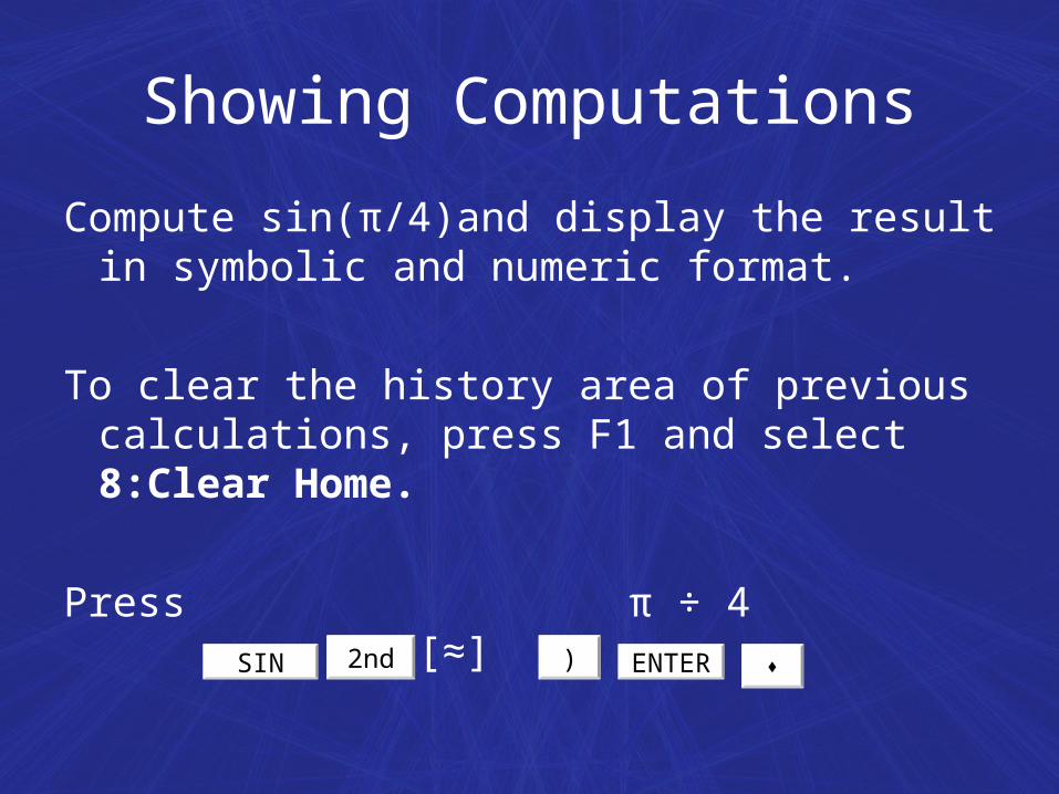
Compute sin(π/4)and display the result in symbolic and numeric format.
To clear the history area of previous calculations, press F1 and select 8:Clear Home.
Press π ÷ 4 [≈]SIN 2nd ) ENTER
Showing Computations

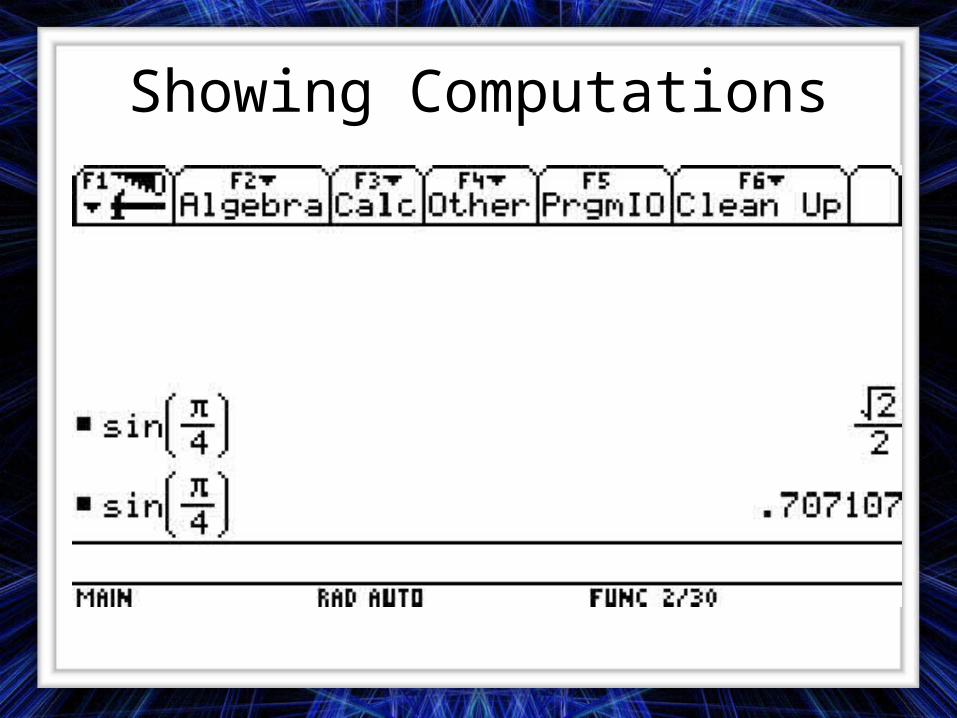
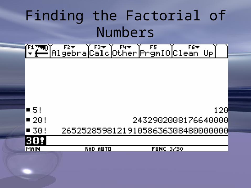
Finding the Factorial of Numbers
Compute the factorial of several number to see how the TI89/Voyage 200 handles very large integers. To get the factorial operator (!) press [MATH], select 7:Probability, and then select 1:!
Press 5 [!] 20 [!] 30
[!]
2nd
2nd ENTER 2nd ENTER 2nd
ENTER
Finding the Factorial of Numbers
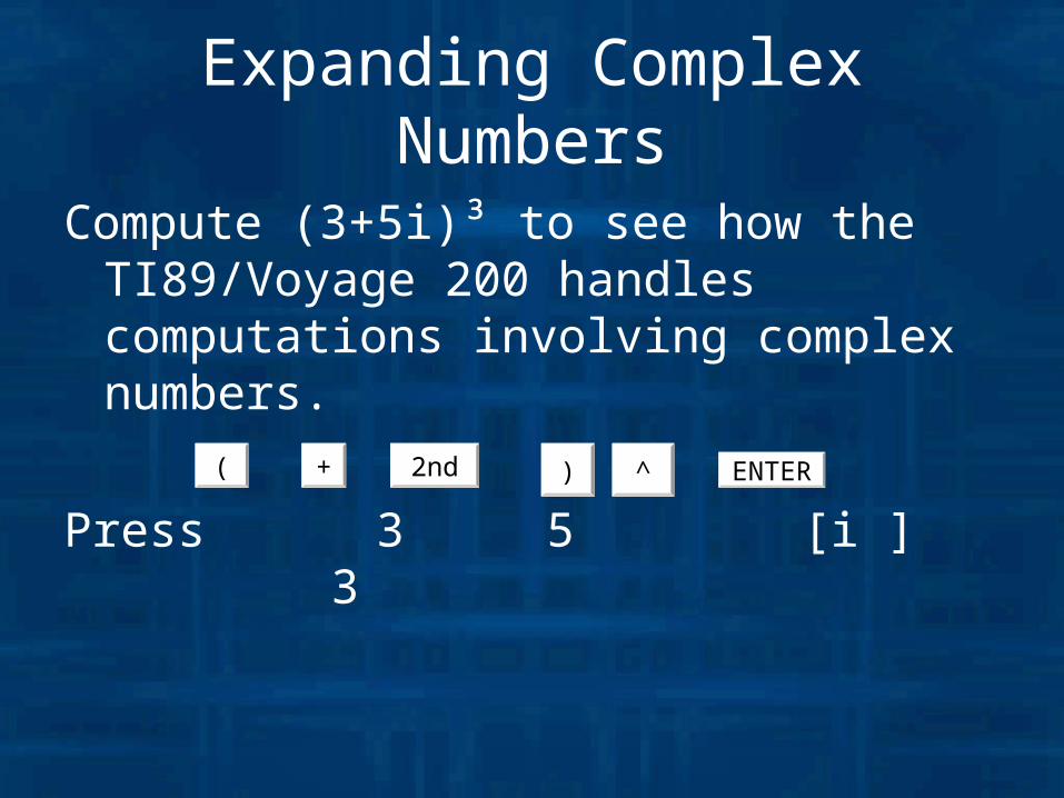
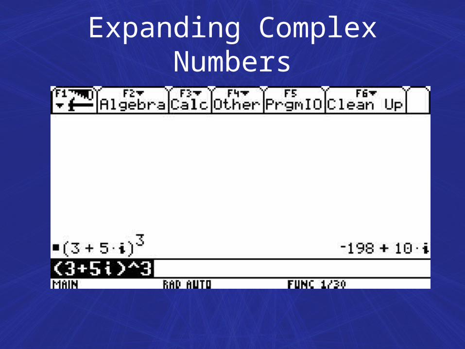
Expanding Complex Numbers
Compute (3+5i)³ to see how the TI89/Voyage 200 handles computations involving complex numbers.
Press 3 5 [i ] 3 ( + 2nd ) ^ ENTER
Expanding Complex Numbers
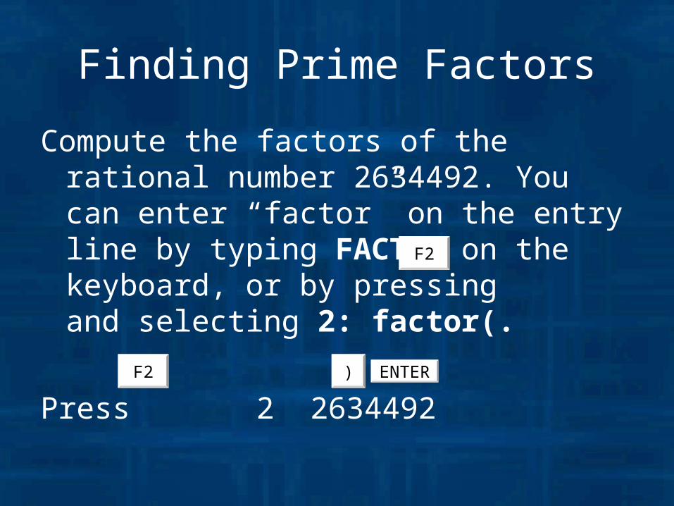
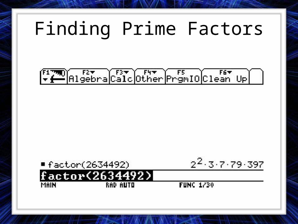
Finding Prime Factors
Compute the factors of the rational number 2634492. You can enter “factor” on the entry line by typing FACTOR on the keyboard, or by pressing and selecting 2: factor(.
Press 2 2634492
F2
F2 ) ENTER
Finding Prime Factors
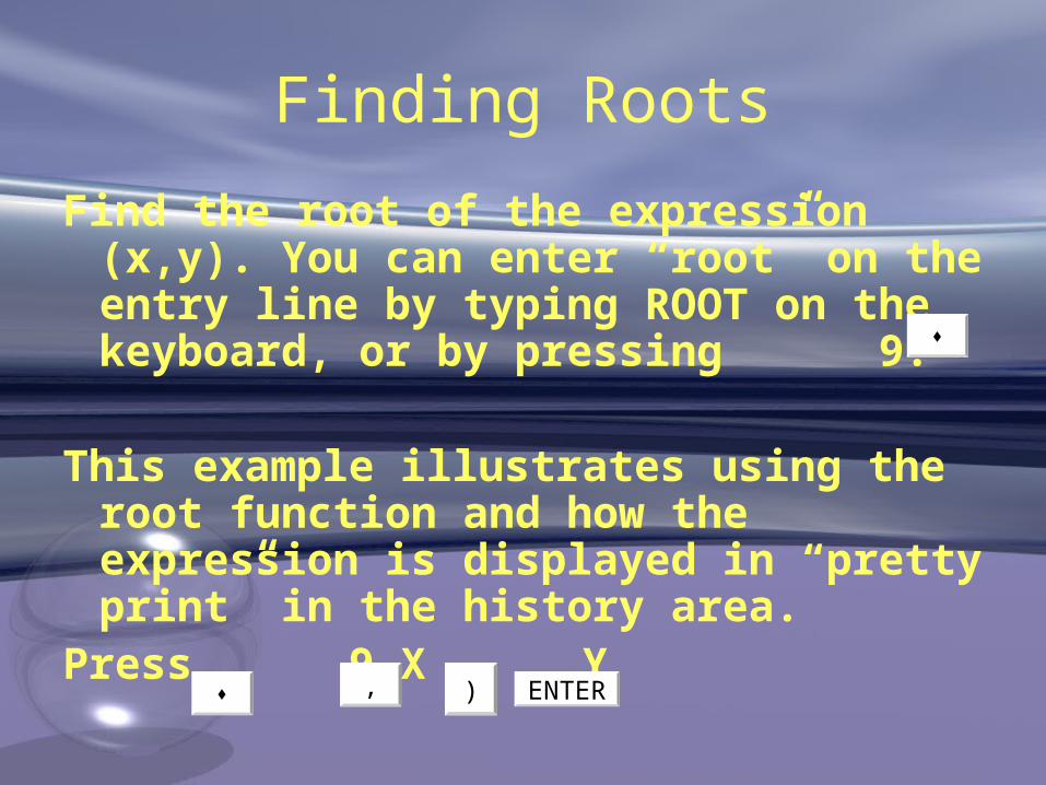
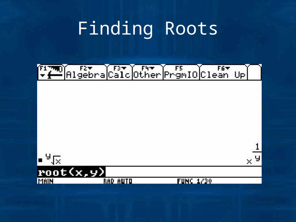
Finding Roots
Find the root of the expression (x,y). You can enter “root” on the entry line by typing ROOT on the keyboard, or by pressing 9.
This example illustrates using the root function and how the expression is displayed in “pretty print” in the history area.
Press 9 X Y
, ) ENTER
Finding Roots
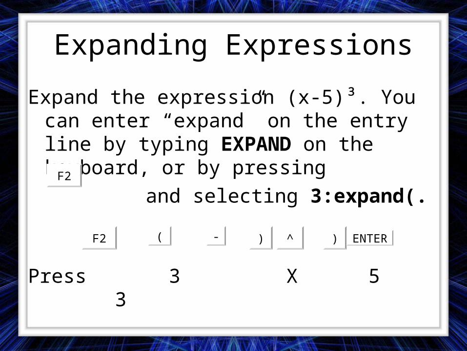
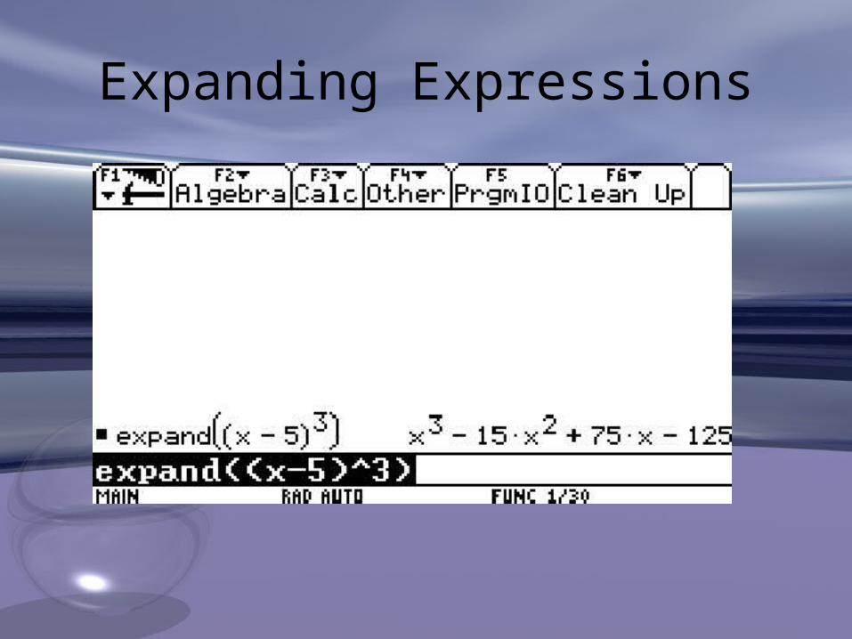
Expanding Expressions
Expand the expression (x-5)³. You can enter “expand” on the entry line by typing EXPAND on the keyboard, or by pressing
and selecting 3:expand(.
Press 3 X 5 3
F2
F2 ( - ) ^ ) ENTER
Expanding Expressions
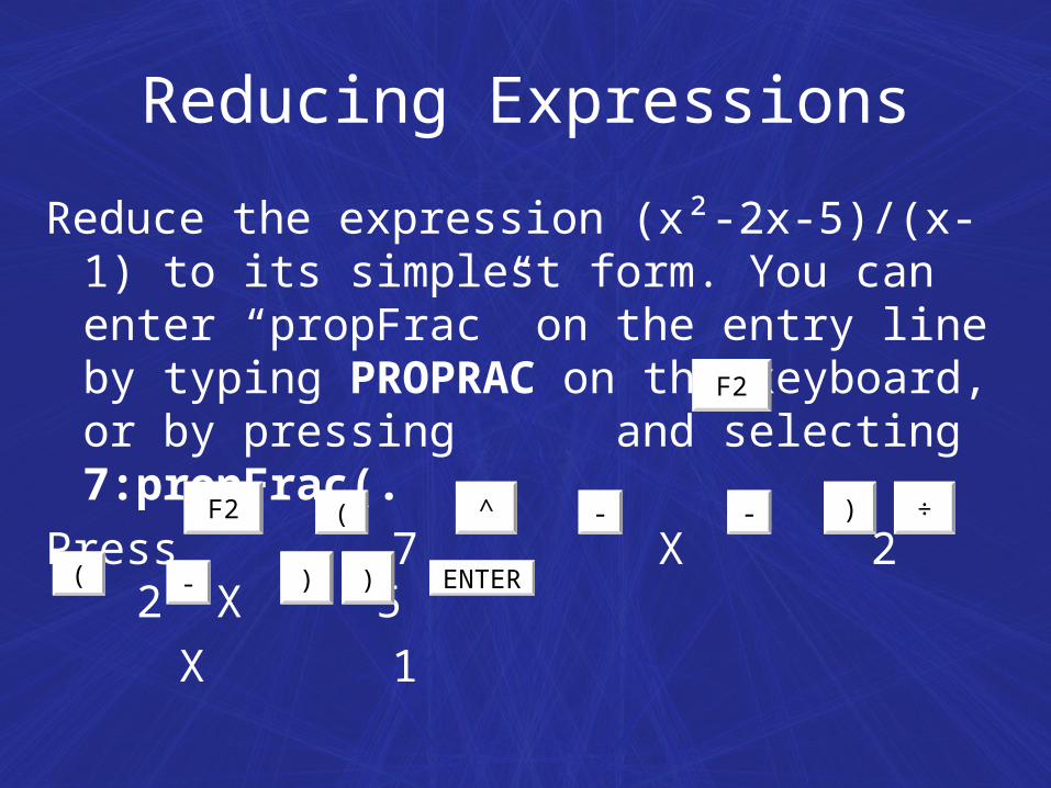
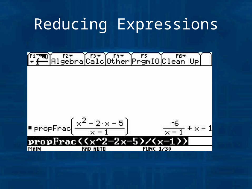
Reducing Expressions
Reduce the expression (x²-2x-5)/(x-1) to its simplest form. You can enter “propFrac” on the entry line by typing PROPRAC on the keyboard, or by pressing and selecting 7:propFrac(.
Press 7 X 2 2 X 5
X 1
F2
F2 ^ - - ) ÷
( - ) ) ENTER
(
Reducing Expressions
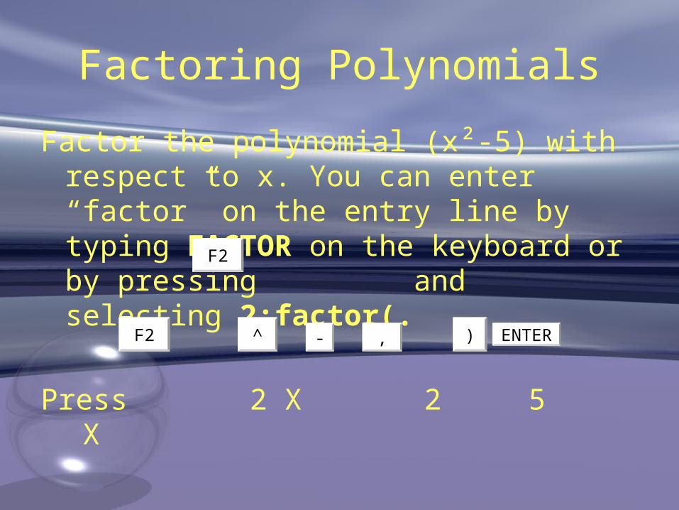
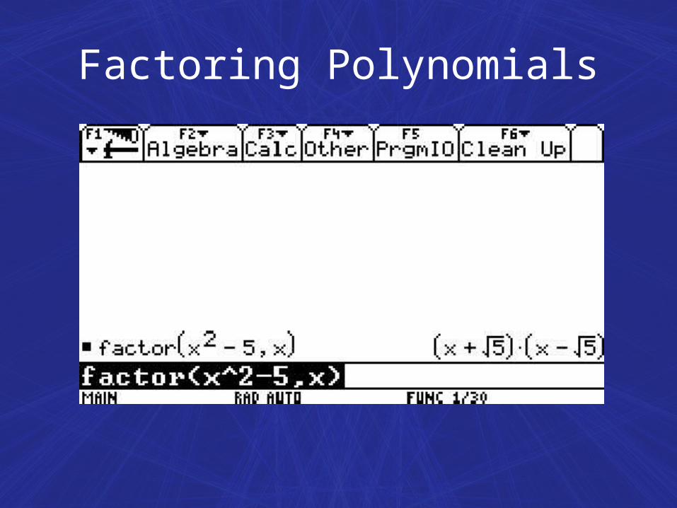
Factoring Polynomials
Factor the polynomial (x²-5) with respect to x. You can enter “factor” on the entry line by typing FACTOR on the keyboard or by pressing and selecting 2:factor(.
Press 2 X 2 5 X
F2
F2 ^ - , ) ENTER
Factoring Polynomials
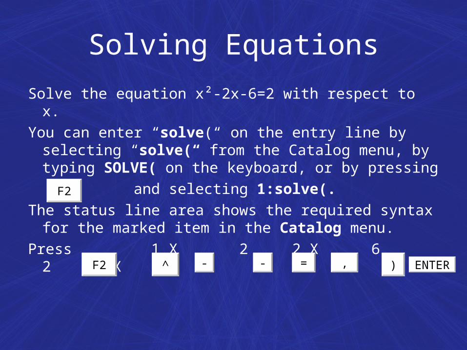
Solving Equations
Solve the equation x²-2x-6=2 with respect to x.
You can enter “solve(“ on the entry line by selecting “solve(“ from the Catalog menu, by typing SOLVE( on the keyboard, or by pressing
and selecting 1:solve(.
The status line area shows the required syntax for the marked item in the Catalog menu.
Press 1 X 2 2 X 6 2 X
F2
F2 ^ - - = , ) ENTER

Solving Equations
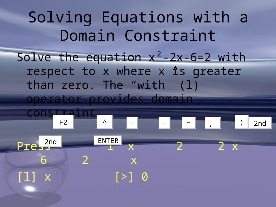
Solving Equations with a Domain Constraint
Solve the equation x²-2x-6=2 with respect to x where x is greater than zero. The “with” (l) operator provides domain constraint.
Press 1 x 2 2 x 6 2 x
[l] x [>] 0
F2 ^ - - = , ) 2nd
2nd ENTER
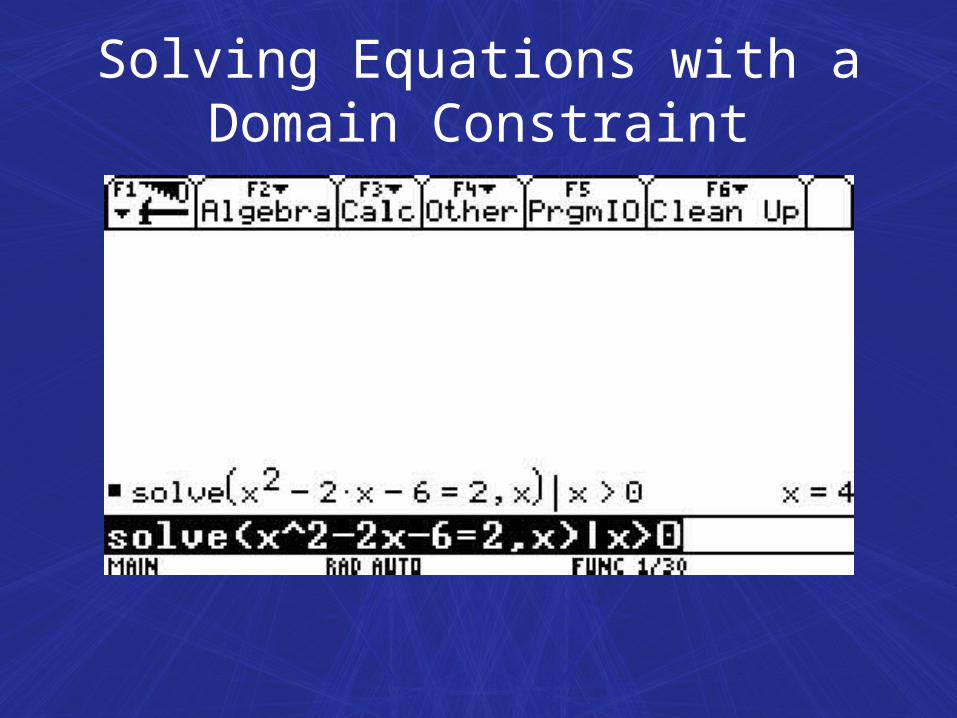
Solving Equations with a Domain Constraint
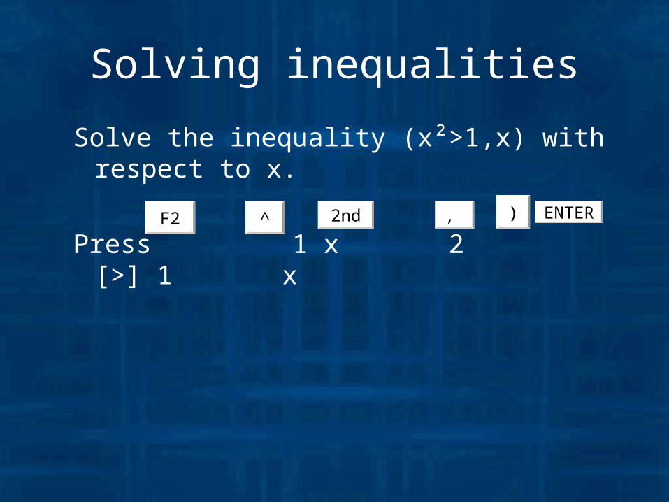
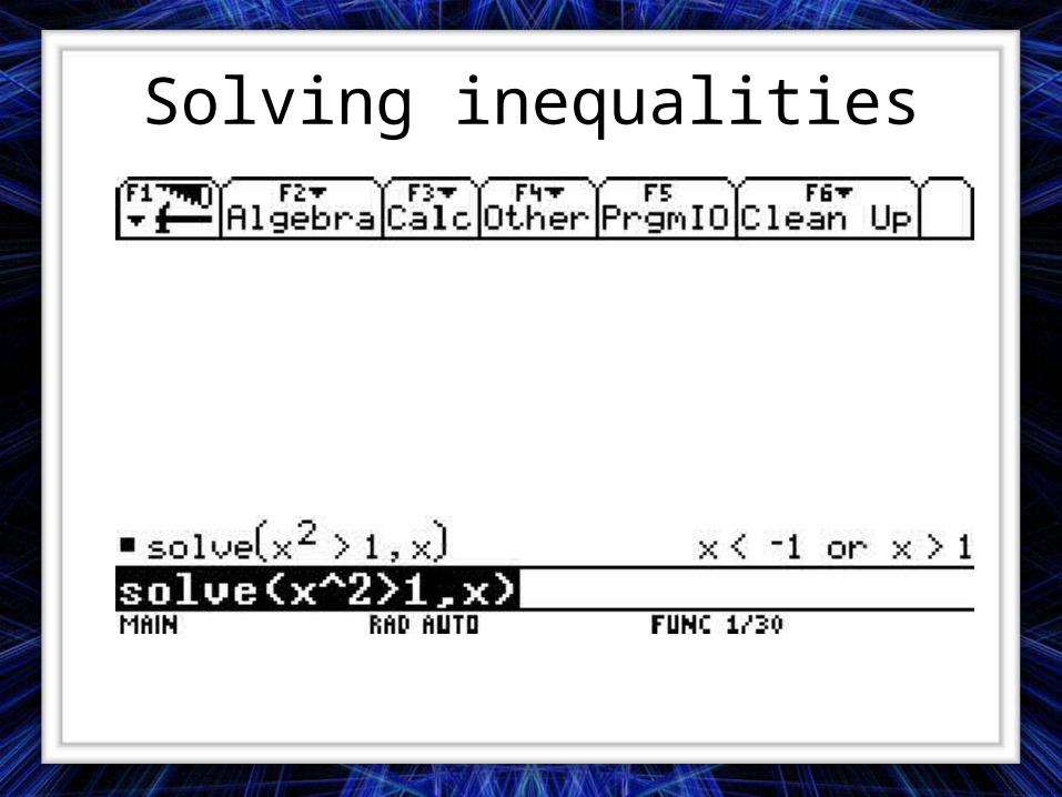
Solving inequalities
Solve the inequality (x²>1,x) with respect to x.
Press 1 x 2 [>] 1 x F2 ^ 2nd , ) ENTER
Solving inequalities
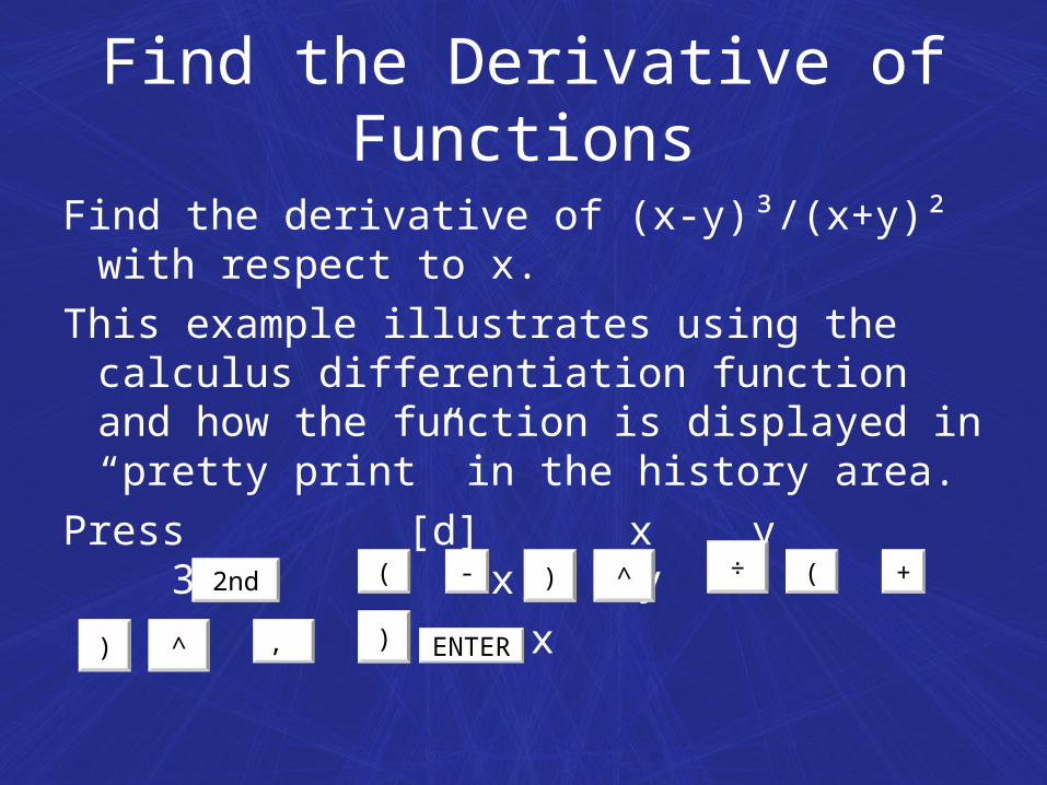
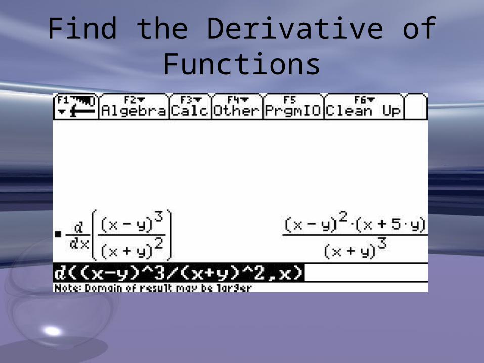
Find the Derivative of Functions
Find the derivative of (x-y)³/(x+y)² with respect to x.
This example illustrates using the calculus differentiation function and how the function is displayed in “pretty print” in the history area.
Press [d] x y 3 x y
2 x
2nd ( - ) ^ ÷ ( +
) ^ , ) ENTER
Find the Derivative of Functions
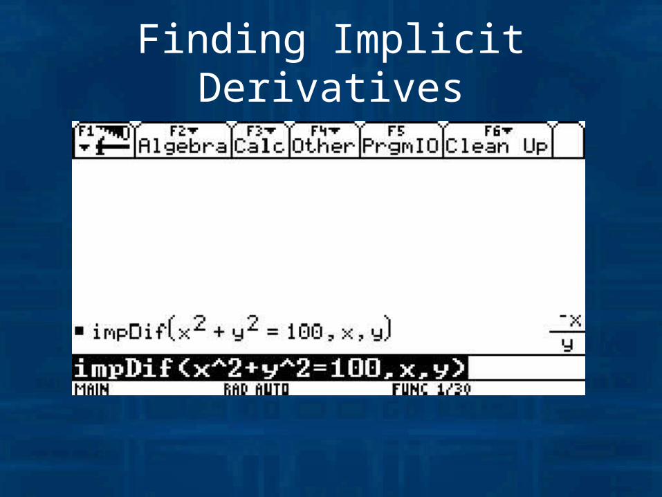
Finding Implicit Derivatives
Compute implicit derivatives for equations in two variables in which one variable is defined implicitly in terms of another.
This example illustrates using the calculus implicit derivative function.
Press D x 2 y 2 100 x yF3 ^ + ^ = , ,
) ENTER
Finding Implicit Derivatives
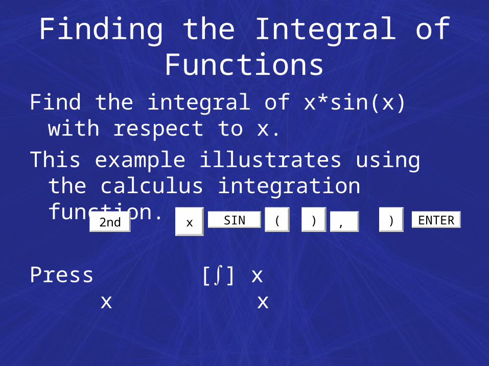
Finding the Integral of Functions
Find the integral of x*sin(x) with respect to x.
This example illustrates using the calculus integration function.
Press [∫] x x x 2nd x SIN ( , ) ENTER)
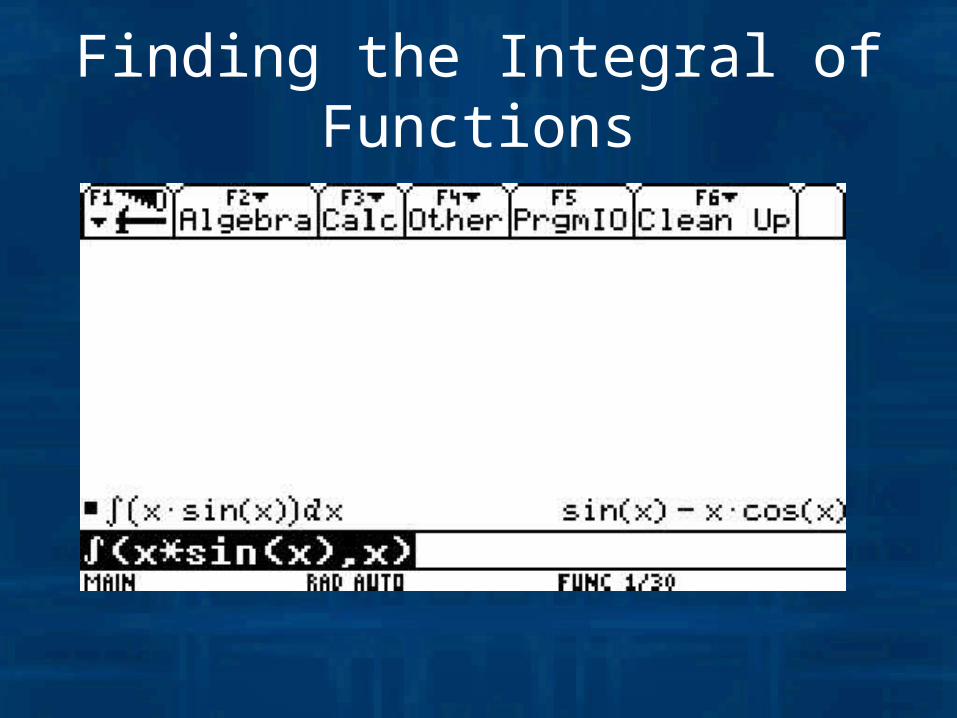
Finding the Integral of Functions
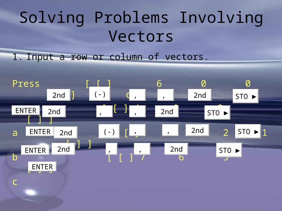
Solving Problems Involving Vectors
1. Input a row or column of vectors.
Press [ [ ] 6 0 0 [ ] ] d
[ [ ] 4 0 2 [ ] ]
a [ [ ] 1 2 1 [ ] ]
b [ [ ] 7 6 5 [ ] ]
c
2nd (-) , , 2nd STO ►
ENTER 2nd , , 2nd STO ►
ENTER 2nd (-) , , 2nd STO ►
ENTER 2nd , , 2nd STO ►
ENTER
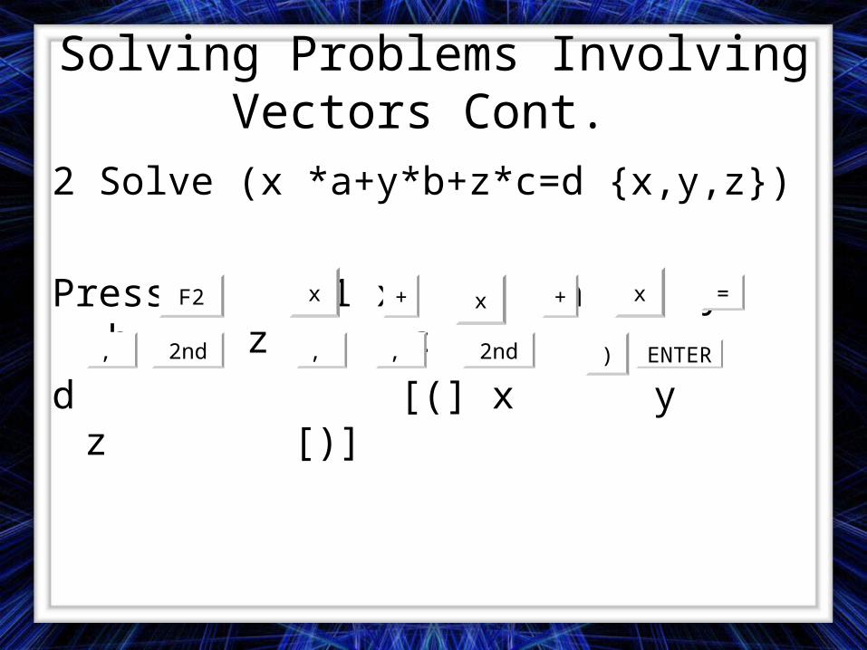
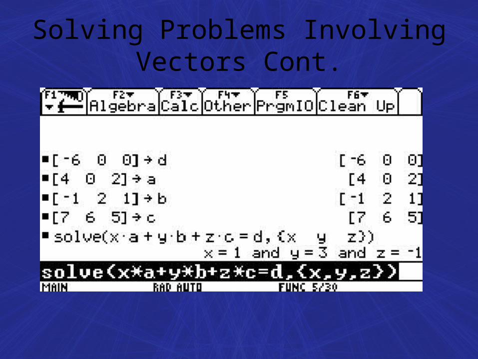
Solving Problems Involving Vectors Cont.
2 Solve (x *a+y*b+z*c=d {x,y,z})
Press 1 x a y b z c
d [(] x y z [)]
F2 x + x + x =
, 2nd , , 2nd ) ENTER
Solving Problems Involving Vectors Cont.
Symbolic Manipulation
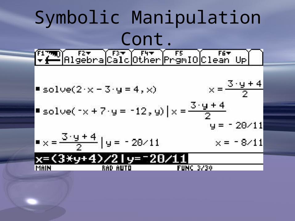
Solve the system of equations 2x-3y=4 and
-x+7y=-12. solve the first equation so the x is expressed in terms of y. Substitute the expression for x into the second equation, and solve for the value of y. Then substitute the y value back into the first equation to solve for the value of x.
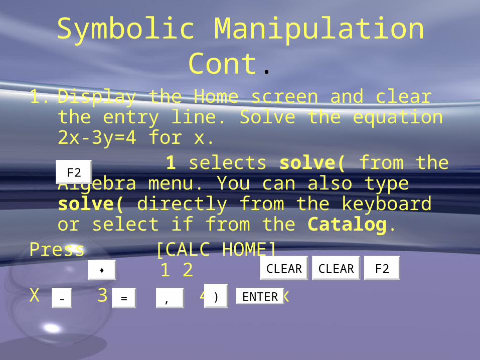
Symbolic Manipulation Cont.
1. Display the Home screen and clear the entry line. Solve the equation 2x-3y=4 for x.
1 selects solve( from the Algebra menu. You can also type solve( directly from the keyboard or select if from the Catalog.
Press [CALC HOME] 1 2 X 3 Y 4 x
F2
CLEAR CLEAR F2
- = , ) ENTER
Symbolic Manipulation Cont.
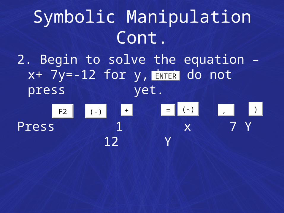
2. Begin to solve the equation –x+ 7y=-12 for y, but do not press yet.
Press 1 x 7 Y 12 Y
ENTER
F2 (-) + = (-) , )
Symbolic Manipulation Cont.
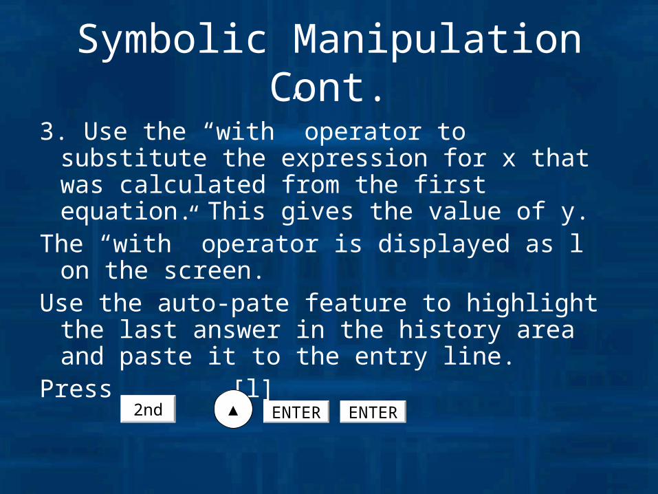
3. Use the “with” operator to substitute the expression for x that was calculated from the first equation. This gives the value of y.
The “with” operator is displayed as l on the screen.
Use the auto-pate feature to highlight the last answer in the history area and paste it to the entry line.
Press [l] 2nd ▲ ENTER ENTER
Symbolic Manipulation Cont.
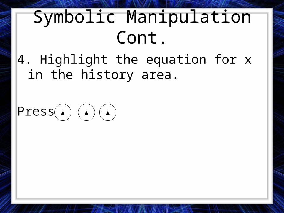
4. Highlight the equation for x in the history area.
Press ▲ ▲ ▲
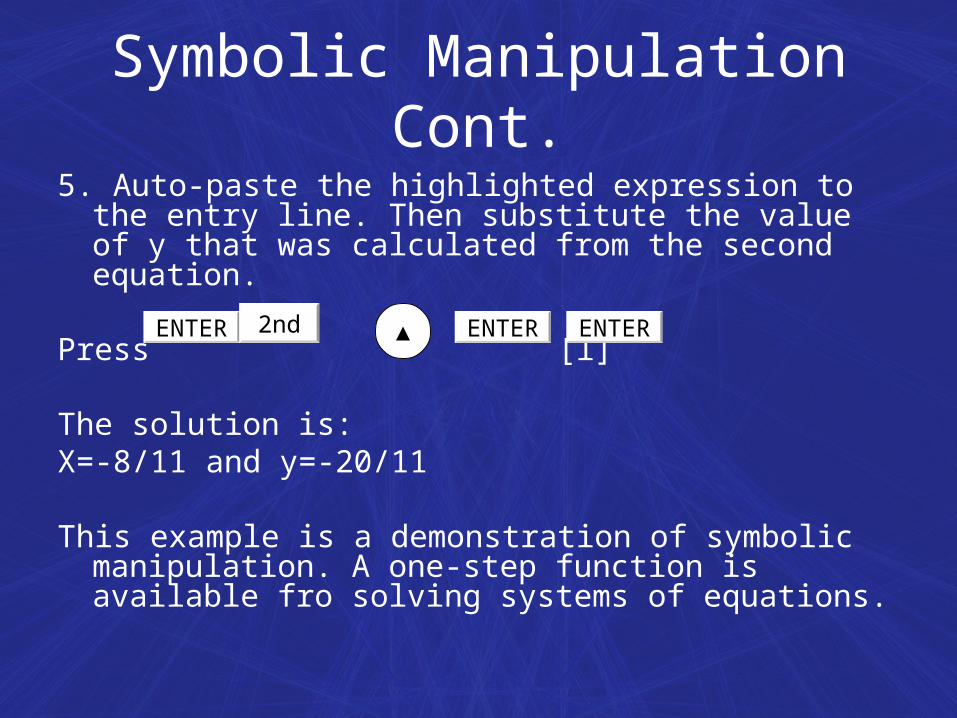
5. Auto-paste the highlighted expression to the entry line. Then substitute the value of y that was calculated from the second equation.
Press [l]
The solution is: X=-8/11 and y=-20/11
This example is a demonstration of symbolic manipulation. A one-step function is available fro solving systems of equations.
Symbolic Manipulation Cont.
ENTER 2nd ▲ ENTER ENTER
Symbolic Manipulation Cont.
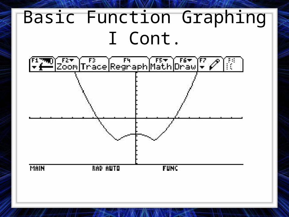
Basic Function Graphing I
The example in this section demonstrates some of the graphing capabilities of the TI/89/Voyage 200 keystrokes. It illustrates how to graph a function using the Y=Editor. You will learn how to enter a function, produce a graph of the function, trace a curve, find a minimum point, and transfer the minimum coordinates to the Home screen. Explore the graphing capabilities of the TI-89/Voyage 200 by graphing the function y=(|x²-3|-10)/2.
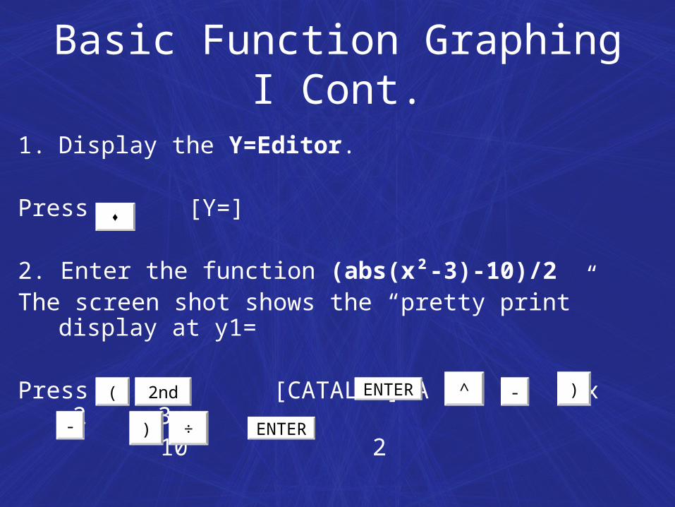
Basic Function Graphing I Cont.
1. Display the Y=Editor.
Press [Y=]
2. Enter the function (abs(x²-3)-10)/2The screen shot shows the “pretty print” display at y1=
Press [CATALOG] A x 2 3 10 2
( 2nd ENTER ^ - )
- ) ÷ ENTER
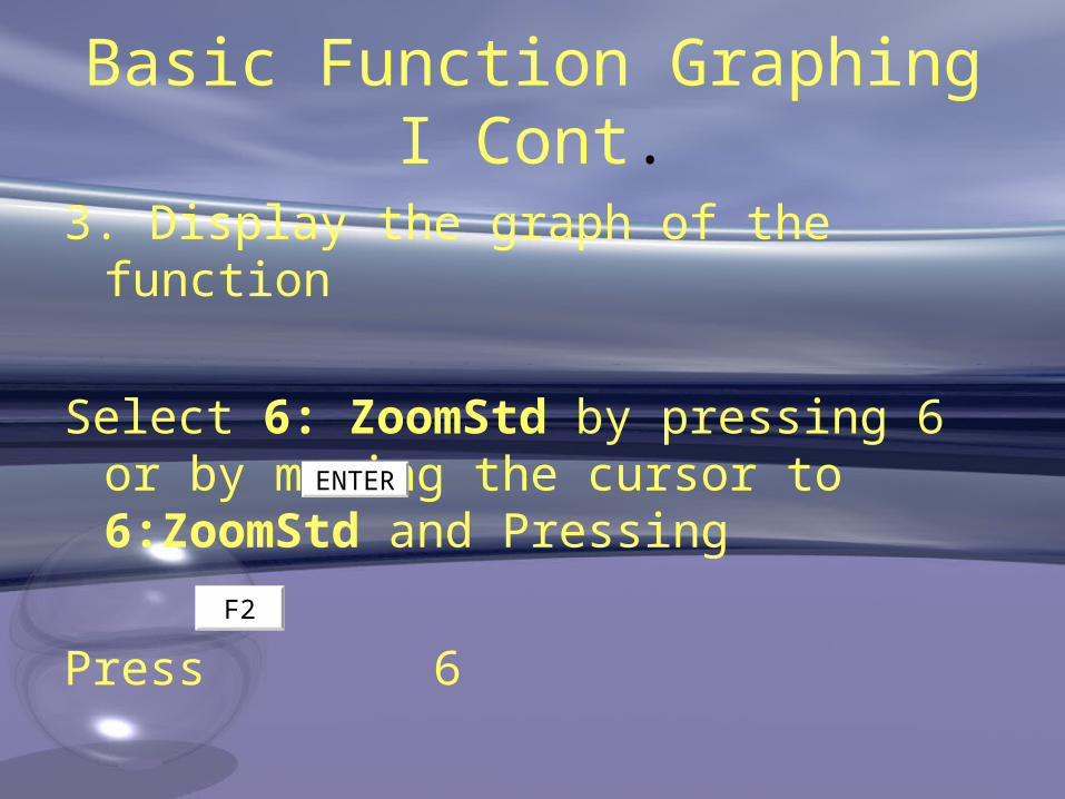
Basic Function Graphing I Cont.
3. Display the graph of the function
Select 6: ZoomStd by pressing 6 or by moving the cursor to 6:ZoomStd and Pressing
Press 6
ENTER
F2
Basic Function Graphing I Cont.
4. Turn on Trace.
The tracing cursor, and the x and y coordinates are displayed.
Press
Basic Function Graphing I Cont.
F3
Basic Function Graphing I Cont.
5. Open the MATH menu and select 3: Minimum.
Press F5 ▼ ▼ ENTER
Basic Function Graphing I Cont.
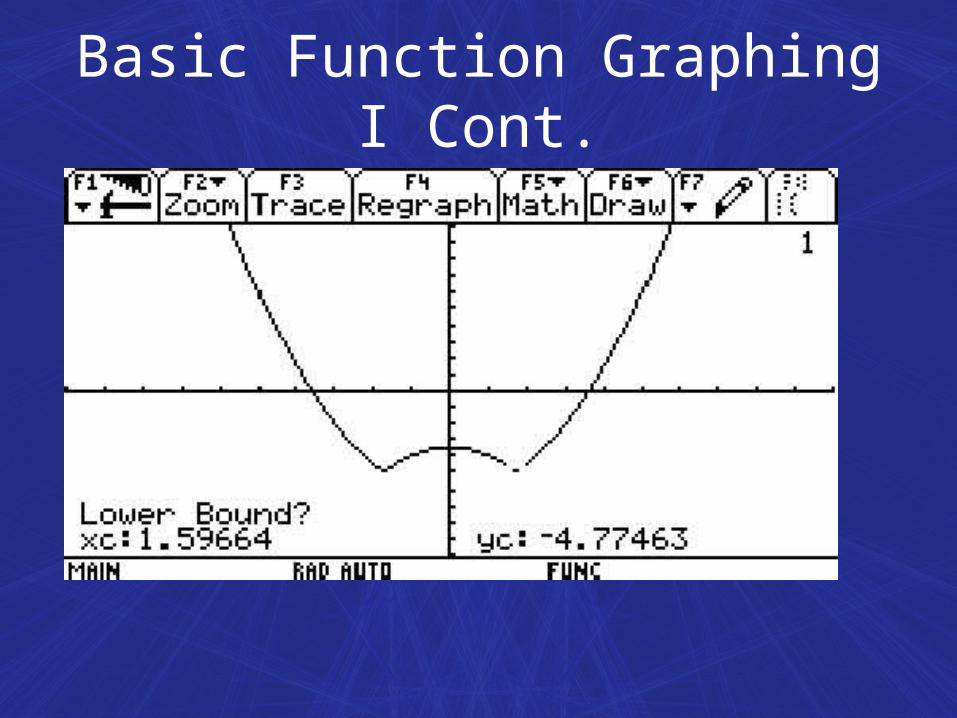
6. Set the lower bound.
Press (right cursor) to move the tracing cursor until the lower bound for x is just to the left of the minimum node before pressing the second time.
Press …
►
ENTER
► ► ENTER
Basic Function Graphing I Cont.
Basic Function Graphing I Cont.
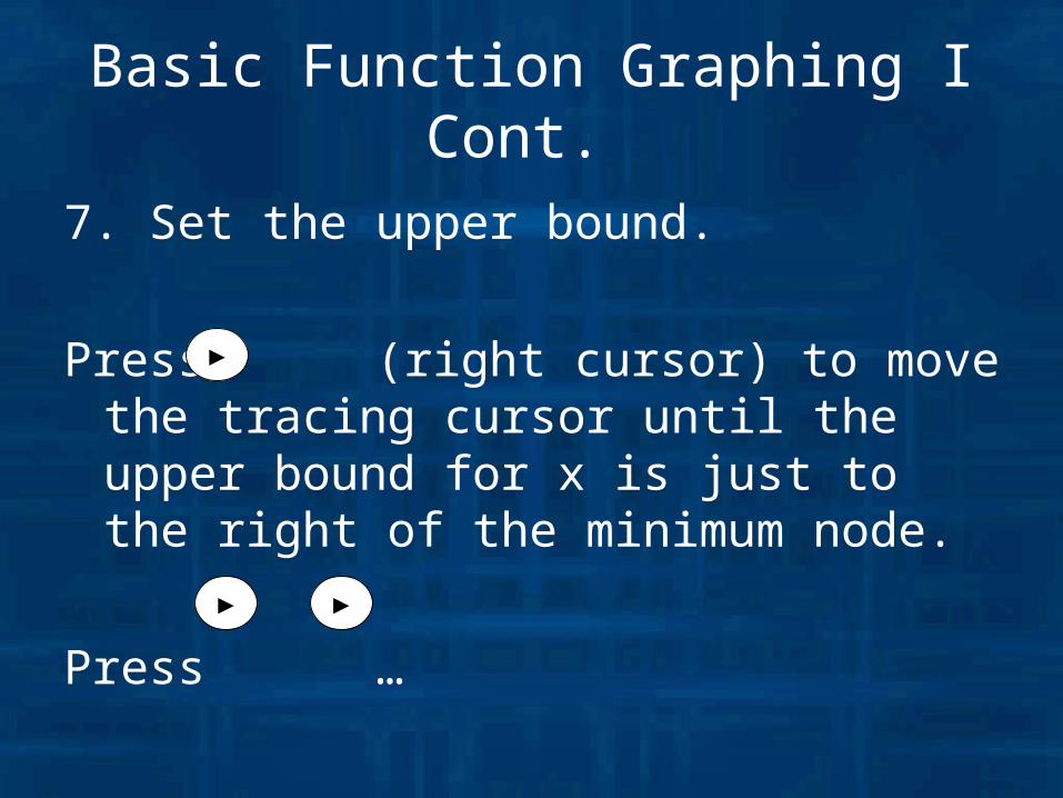
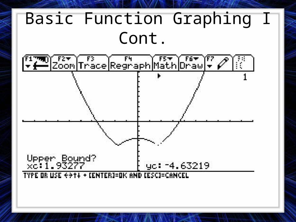
7. Set the upper bound.
Press (right cursor) to move the tracing cursor until the upper bound for x is just to the right of the minimum node.
Press …
►
► ►
Basic Function Graphing I Cont.
Basic Function Graphing I Cont.
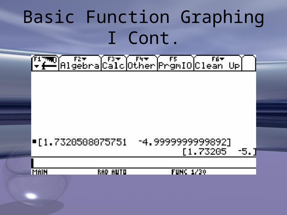
8. Find the minimum point on the graph between the lower and upper bounds.
Press ENTER
Basic Function Graphing I Cont.
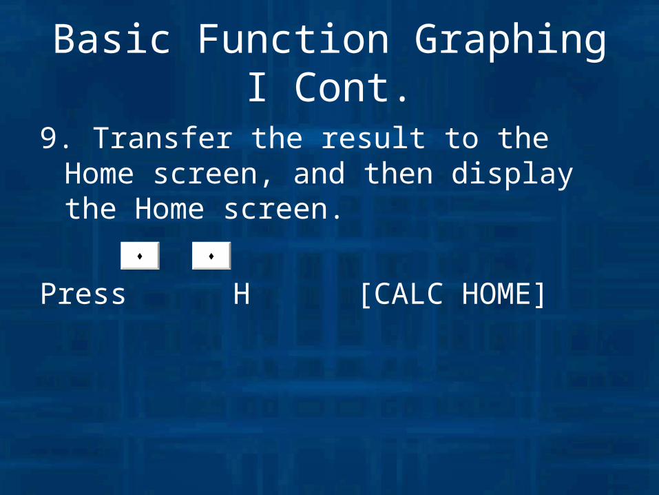
9. Transfer the result to the Home screen, and then display the Home screen.
Press H [CALC HOME]
Basic Function Graphing I Cont.
Basic Function Graphing II
Graph a circle of radius 5, centered on the origin of the coordinate system. View the circle using the standard viewing window (ZoomStd). Then use ZoomSqr to adjust the viewing window.
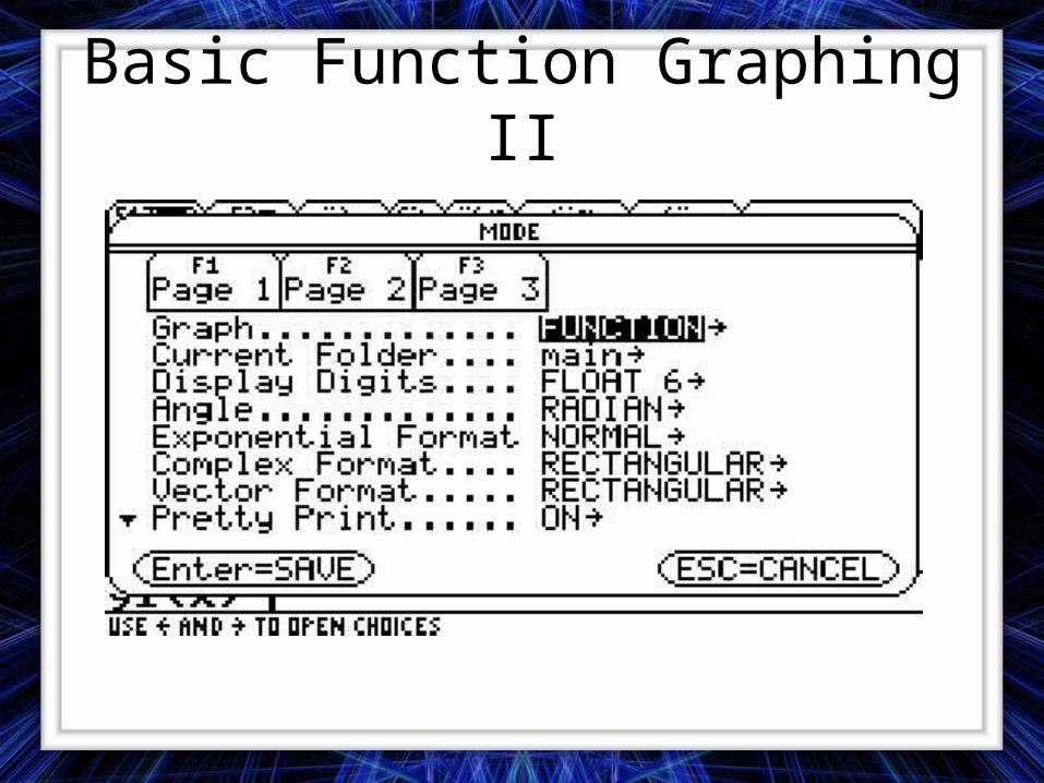
1. Display the MODE dialog box. For Graph mode, select Function
Press 1 MODE ► ENTER
Basic Function Graphing II
Basic Function Graphing II Cont.
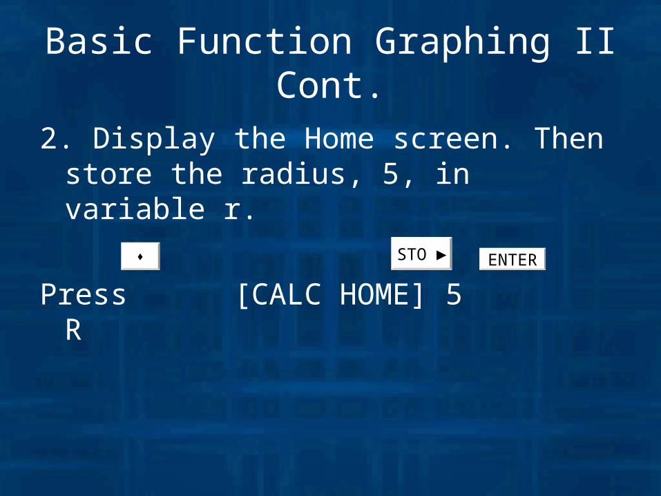
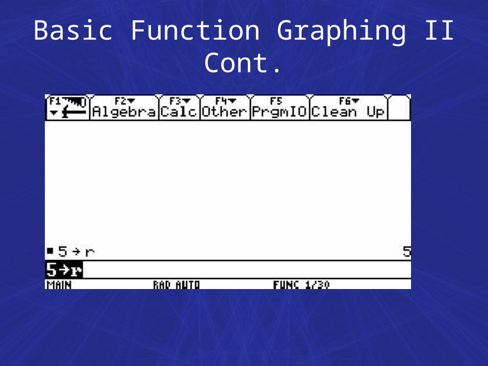
2. Display the Home screen. Then store the radius, 5, in variable r.
Press [CALC HOME] 5 R STO ► ENTER
Basic Function Graphing II Cont.
Basic Function Graphing II Cont.
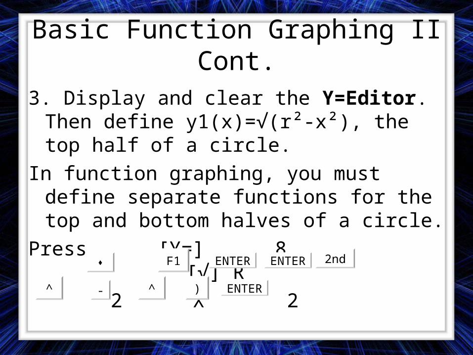
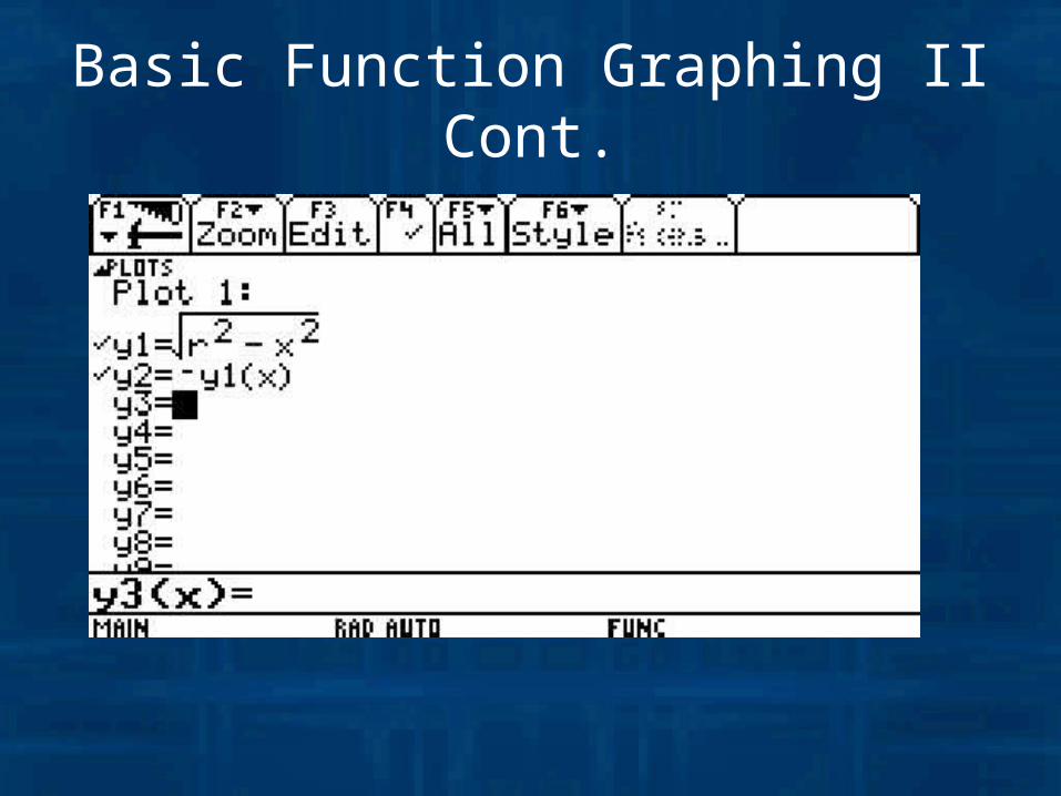
3. Display and clear the Y=Editor. Then define y1(x)=√(r²-x²), the top half of a circle.
In function graphing, you must define separate functions for the top and bottom halves of a circle.
Press [Y=] 8 [√] R
2 X 2
F1 ENTER ENTER 2nd
^ - ^ ) ENTER
Basic Function Graphing II Cont.
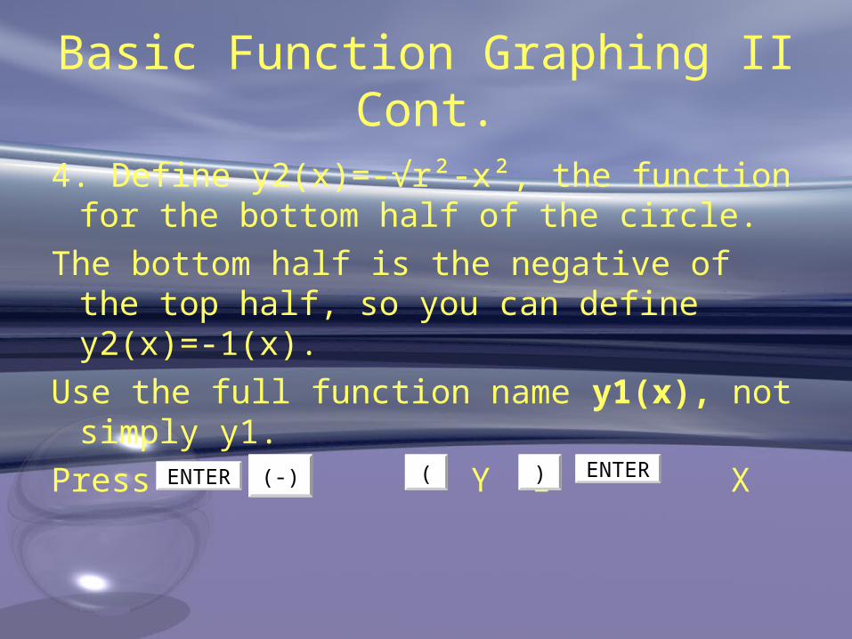
4. Define y2(x)=-√r²-x², the function for the bottom half of the circle.
The bottom half is the negative of the top half, so you can define y2(x)=-1(x).
Use the full function name y1(x), not simply y1.
Press Y 1 X ENTER (-) ( ) ENTER
Basic Function Graphing II Cont.
Basic Function Graphing II Cont.
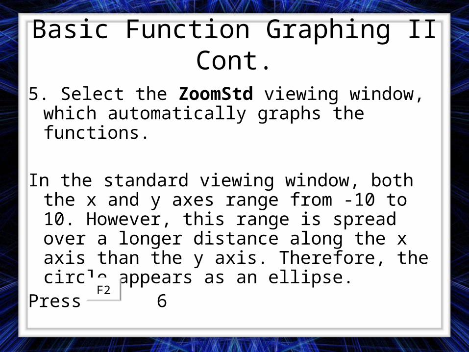
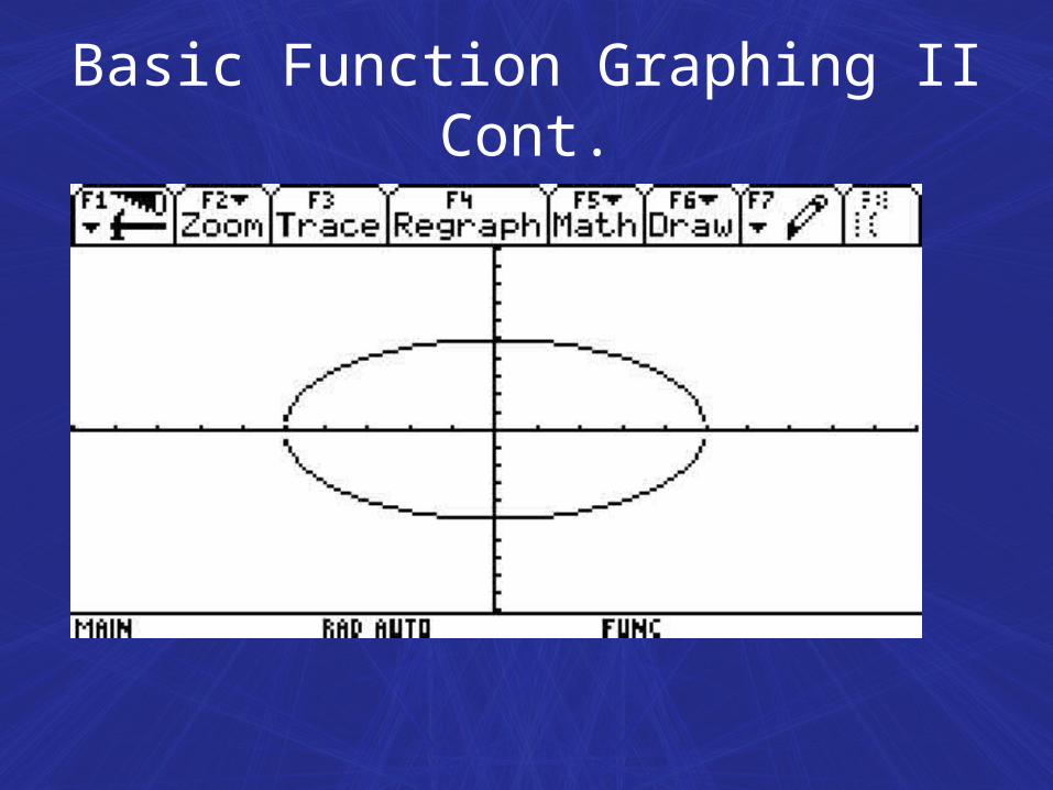
5. Select the ZoomStd viewing window, which automatically graphs the functions.
In the standard viewing window, both the x and y axes range from -10 to 10. However, this range is spread over a longer distance along the x axis than the y axis. Therefore, the circle appears as an ellipse.
Press 6F2
Basic Function Graphing II Cont.
Basic Function Graphing II Cont.
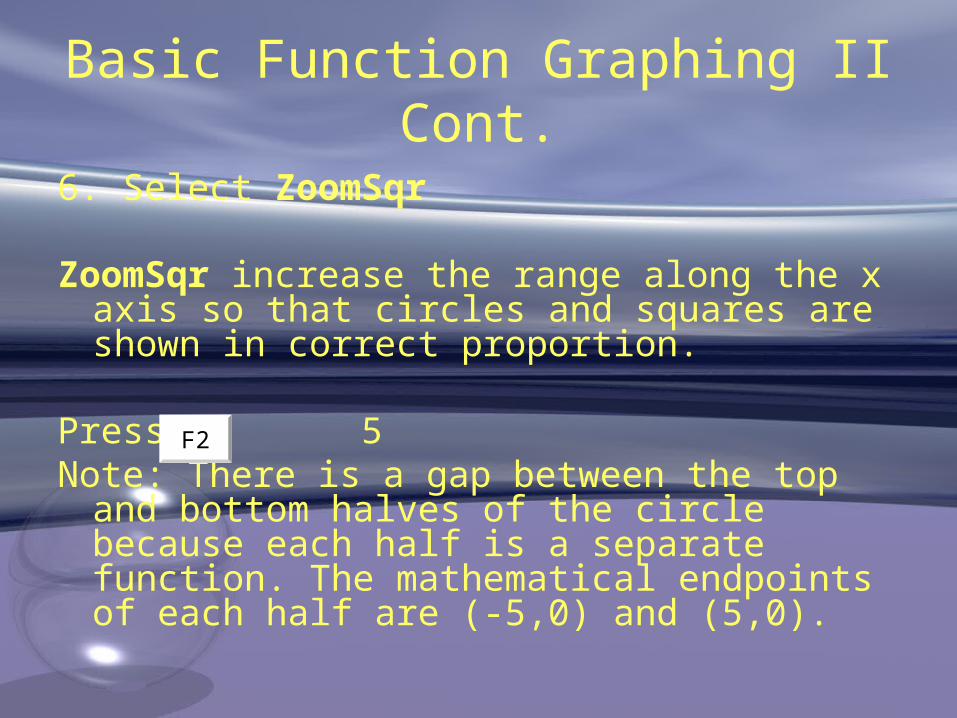
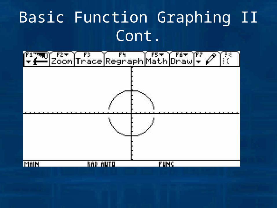
6. Select ZoomSqr
ZoomSqr increase the range along the x axis so that circles and squares are shown in correct proportion.
Press 5Note: There is a gap between the top and bottom
halves of the circle because each half is a separate function. The mathematical endpoints of each half are (-5,0) and (5,0).
F2
Basic Function Graphing II Cont.
Basic Function Graphing III
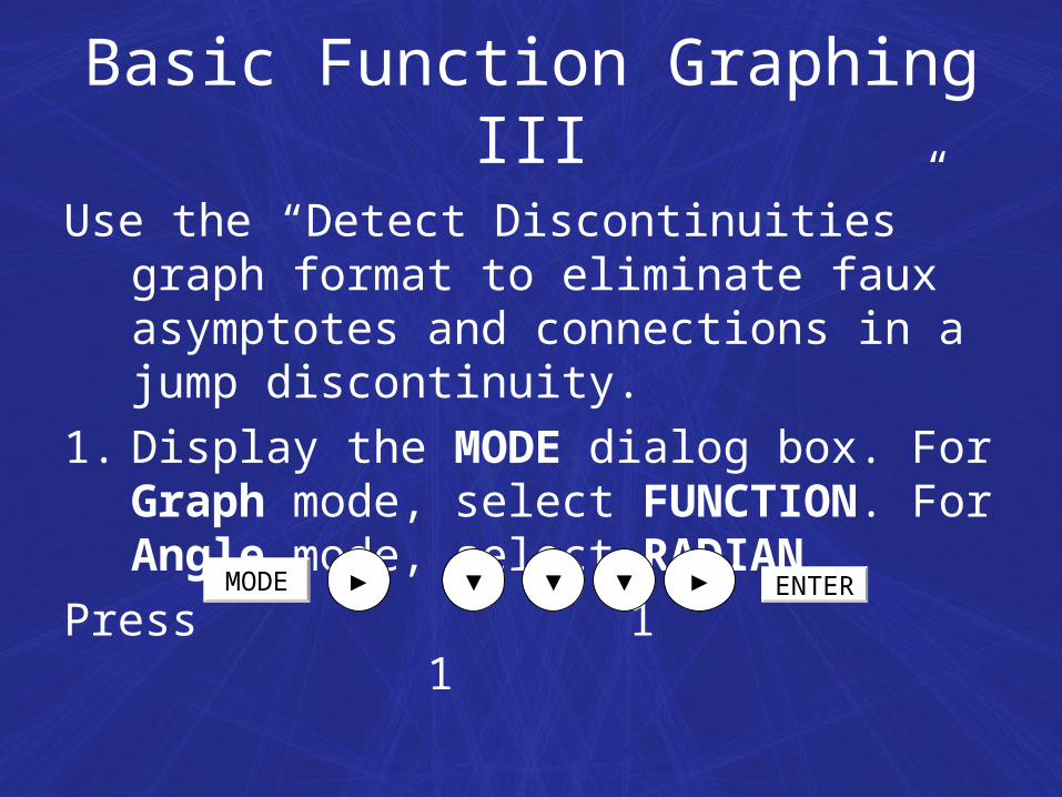
Use the “Detect Discontinuities” graph format to eliminate faux asymptotes and connections in a jump discontinuity.
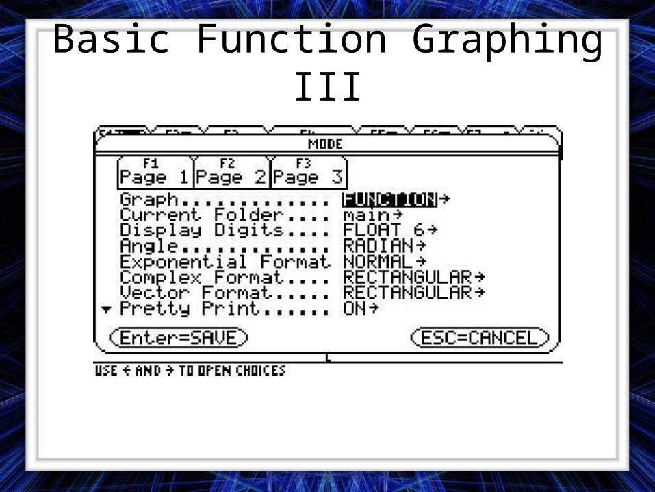
1. Display the MODE dialog box. For Graph mode, select FUNCTION. For Angle mode, select RADIAN
Press 1 1 MODE ► ▼ ▼ ▼ ► ENTER
Basic Function Graphing III
Basic Function Graphing III Cont.
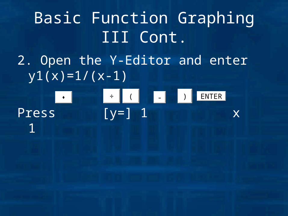
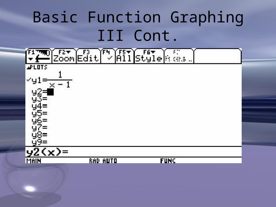
2. Open the Y-Editor and enter y1(x)=1/(x-1)
Press [y=] 1 x 1 ÷ ( - ) ENTER
Basic Function Graphing III Cont.
Basic Function Graphing III Cont.
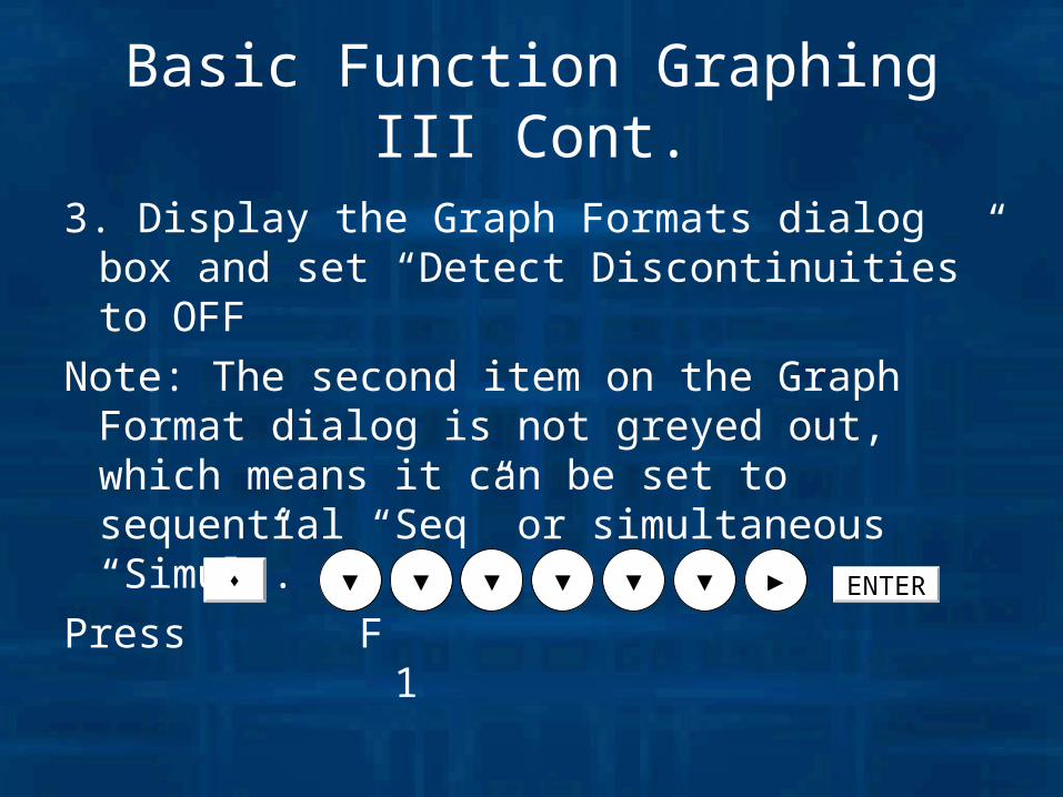
3. Display the Graph Formats dialog box and set “Detect Discontinuities” to OFF
Note: The second item on the Graph Format dialog is not greyed out, which means it can be set to sequential “Seq” or simultaneous “Simul”.
Press F 1 ▼ ▼ ▼ ▼ ▼ ▼ ► ENTER
Basic Function Graphing III Cont.
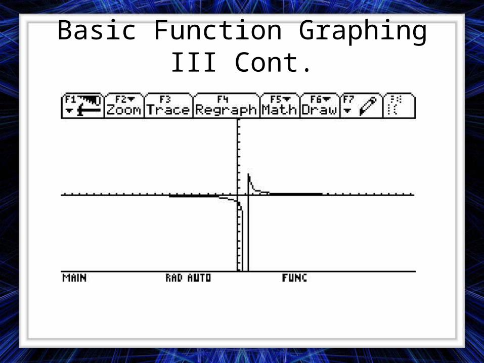
4. Execute the Graph command, which automatically displays the Graph screen. Observe the “faux” asymptotes contained in the graph.
Press [GRAPH]
Basic Function Graphing III Cont.
Basic Function Graphing III Cont.
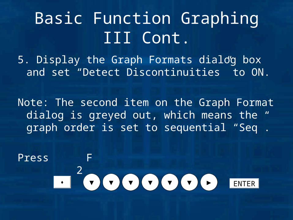
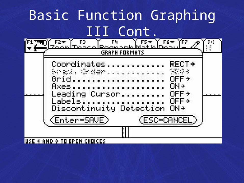
5. Display the Graph Formats dialog box and set “Detect Discontinuities” to ON.
Note: The second item on the Graph Format dialog is greyed out, which means the graph order is set to sequential “Seq”.
Press F 2 ▼ ▼ ▼ ▼ ▼ ▼ ► ENTER
Basic Function Graphing III Cont.
Basic Function Graphing III Cont.
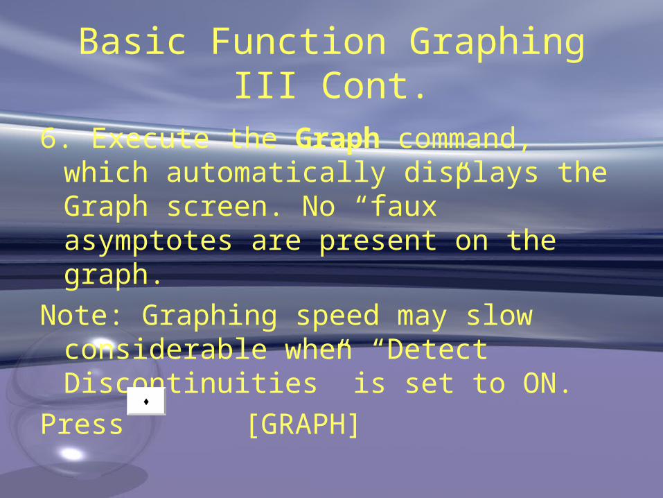
6. Execute the Graph command, which automatically displays the Graph screen. No “faux” asymptotes are present on the graph.
Note: Graphing speed may slow considerable when “Detect Discontinuities” is set to ON.
Press [GRAPH]

Basic Function Graphing III Cont.
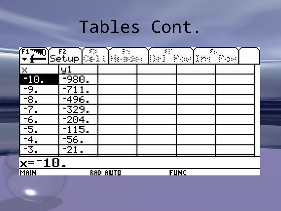
Tables
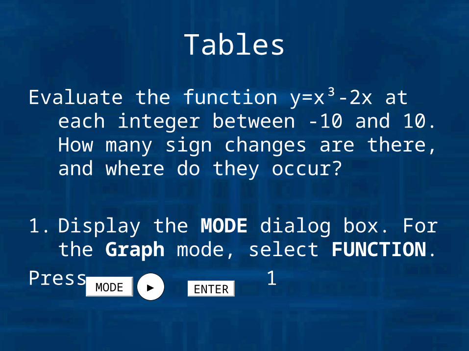
Evaluate the function y=x³-2x at each integer between -10 and 10. How many sign changes are there, and where do they occur?
1. Display the MODE dialog box. For the Graph mode, select FUNCTION.
Press 1MODE ► ENTER
Tables Cont.
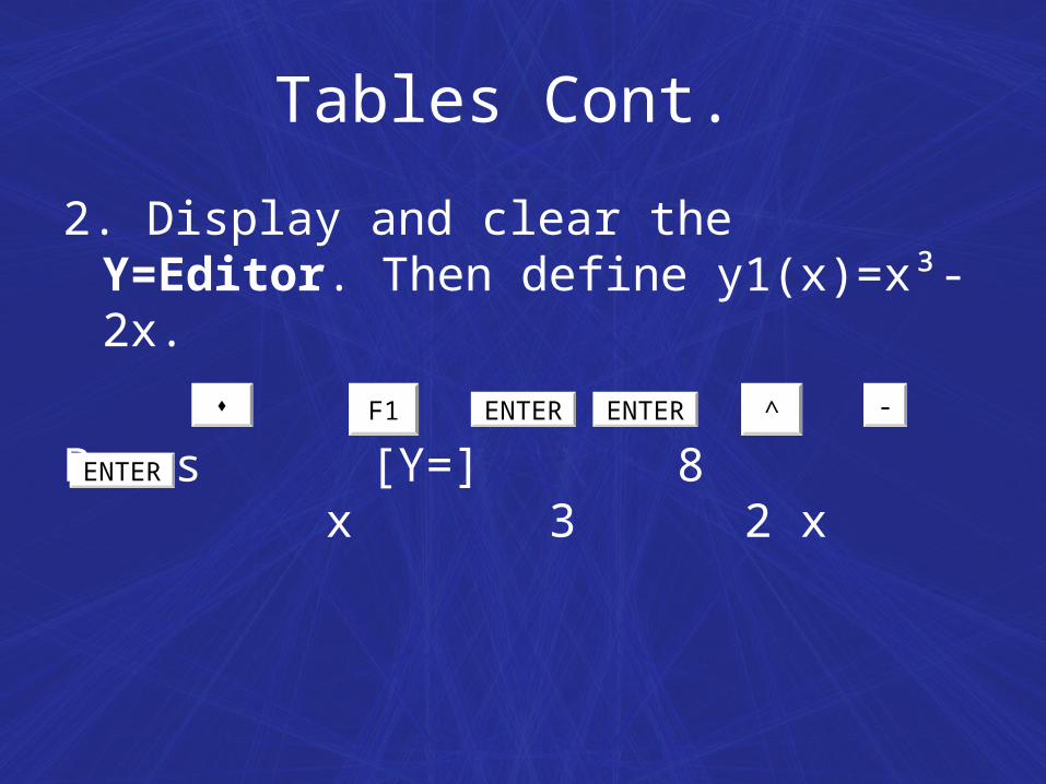
2. Display and clear the Y=Editor. Then define y1(x)=x³-2x.
Press [Y=] 8 x 3 2 x F1 ENTERENTER ^ -
ENTER
Tables Cont.
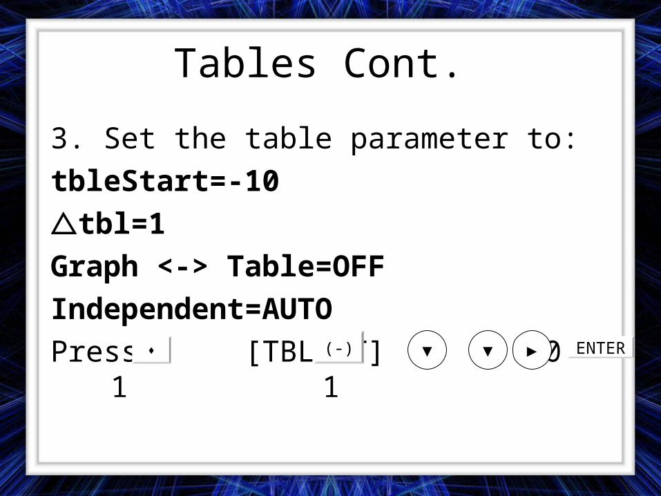
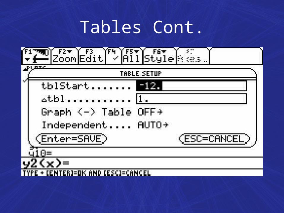
3. Set the table parameter to:
tbleStart=-10
tbl=1
Graph <-> Table=OFF
Independent=AUTO
Press [TBLSET] 10 1 1 (-) ▼ ▼ ► ENTER
Tables Cont.
Tables Cont.
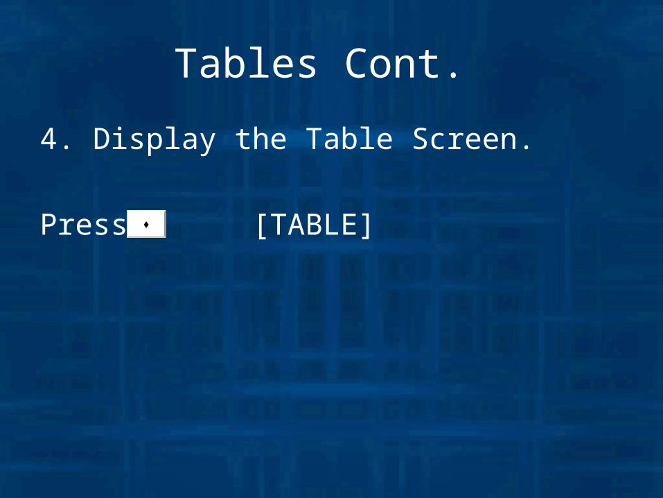
4. Display the Table Screen.
Press [TABLE]
Tables Cont.
Tables Cont.
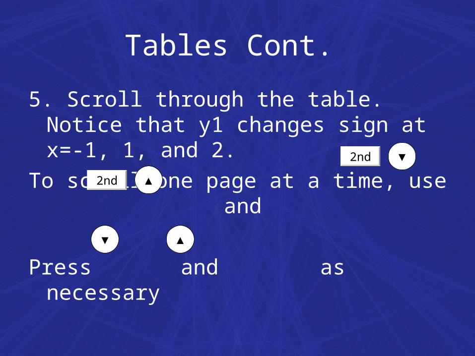
5. Scroll through the table. Notice that y1 changes sign at x=-1, 1, and 2.
To scroll one page at a time, use and
Press and as necessary
2nd ▼
2nd ▲
▼ ▲
Tables Cont.
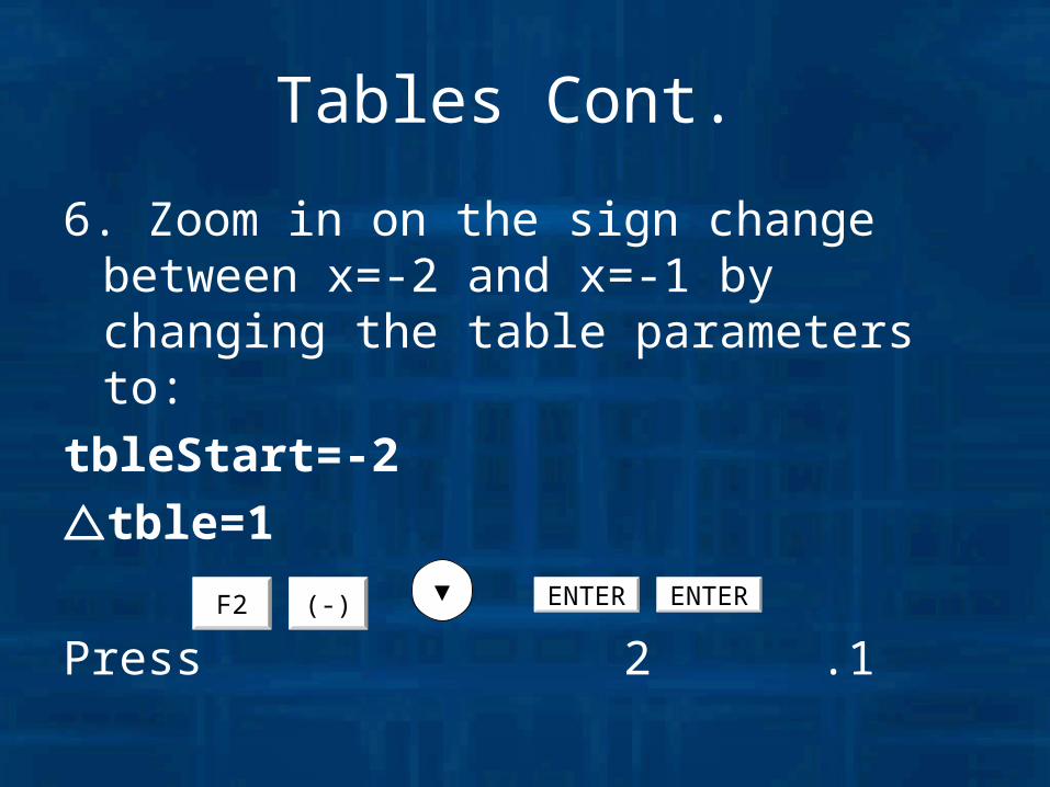
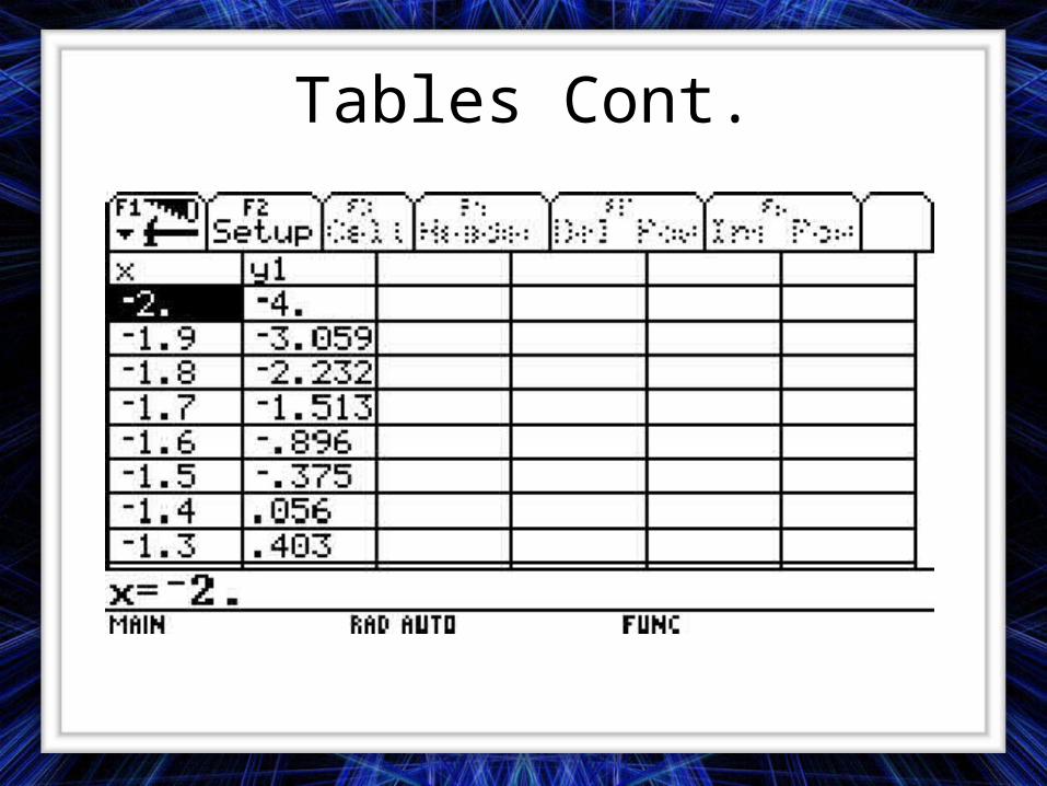
6. Zoom in on the sign change between x=-2 and x=-1 by changing the table parameters to:
tbleStart=-2
tble=1
Press 2 .1 F2 (-) ▼ ENTERENTER
Tables Cont.
Source
Texas Instrument's Previews “Performing Calculations”
Pictures from Andy’s Voyage 200 Texas Instrument
Slides made by Amanda Griffin