This Dissertation 2 - University of Notre DameThis Dissertation entitled EVENT TRIGGERED STATE...

This Dissertation

entitled

EVENT TRIGGERED STATE ESTIMATION AND CONTROL WITH LIMITED

COMMUNICATION

typeset with nddiss2ε v3.2013 (2013/04/16) on June 14, 2013 for

Lichun Li

This LATEX2ε classfile conforms to the University of Notre Dame style guidelines asof Fall 2012. However it is still possible to generate a non-conformant document ifthe instructions in the class file documentation are not followed!

Be sure to refer to the published Graduate School guidelinesat http://graduateschool.nd.edu as well. Those guidelinesoverride everything mentioned about formatting in the docu-mentation for this nddiss2ε class file.

It is YOUR responsibility to ensure that the Chapter titles and Table caption titlesare put in CAPS LETTERS. This classfile does NOT do that!

This page can be disabled by specifying the “noinfo” option to the class invocation.(i.e.,\documentclass[...,noinfo]nddiss2e )

This page is NOT part of the dissertation/thesis. It shouldbe disabled before making final, formal submission, butshould be included in the version submitted for format

check.

nddiss2ε documentation can be found at these locations:

http://www.gsu.nd.edu

http://graduateschool.nd.edu


COMMUNICATION

A Dissertation

Submitted to the Graduate School

of the University of Notre Dame

in Partial Fulfillment of the Requirements

for the Degree of

Doctor of Philosophy

by

Lichun Li

Michael Lemmon, Director

Graduate Program in Department of Electrical Engineering

Notre Dame, Indiana

June 2013


COMMUNICATION

Abstract

by

Lichun Li

Control systems are becoming more efficient, more sustainable and less costly

by the convergence with networking and information technology. The limitation of

transmission frequency and instantaneous bit-rate on most networks, however, can

degrade or even destroy control systems. To maintain system performance with the

limited transmission frequency and limited instantaneous bit-rate, event triggered

transmission, with which transmission is triggered by a certain event, is proposed.

Our research is to analytically examine the tradeoff among system performance,

transmission frequency, and instantaneous bit-rate in event triggered systems.

We first study the optimal communication rule which minimizes mean square

state estimation error with limited transmission frequency. It is shown that the opti-

mal communication rule is event triggered transmission. Because the optimal event

trigger is difficult to compute, computationally efficient suboptimal event trigger is

presented. Our simulation results show that we can compute tighter upper bounds

on the suboptimal costs and tighter lower bounds on the optimal costs than prior

work, while guaranteeing comparative actual costs. Based on the same idea, com-

putationally efficient weakly coupled suboptimal event triggers are also designed for

output feedback control systems to minimize the mean square state with limited

transmission frequency.

Lichun Li

The work above, however, only considers limited transmission frequency. We,

then, consider both the limited transmission frequency and limited instantaneous

bit-rate in event triggered control systems to guarantee input-to-state stability and re-

silience, respectively. To guarantee input-to-state stability, a minimum inter-sampling

interval and a sufficient instantaneous bit-rate are provided. Besides, we also give a

sufficient condition of efficient attentiveness, i.e. longer inter-sampling interval and

lower instantaneous bit-rate can be achieved when the system state gets closer to

the origin. To guarantee resilience to transient unknown magnitude disturbance, de-

tailed algorithms and required sufficient instantaneous bit-rate are presented. Our

simulation results demonstrate the resilience of event triggered systems to transient

unknown magnitude disturbances.

CONTENTS

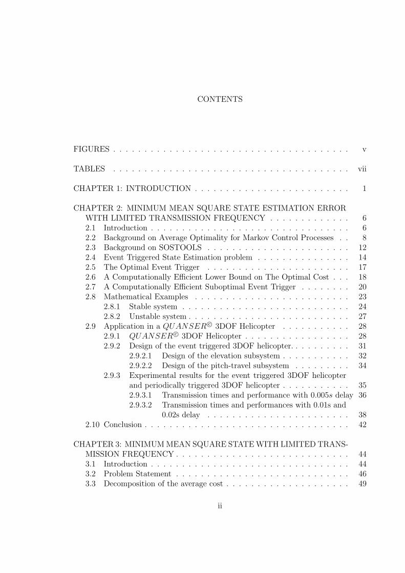
FIGURES . . . . . . . . . . . . . . . . . . . . . . . . . . . . . . . . . . . . . . v

TABLES . . . . . . . . . . . . . . . . . . . . . . . . . . . . . . . . . . . . . . vii

CHAPTER 1: INTRODUCTION . . . . . . . . . . . . . . . . . . . . . . . . . 1

CHAPTER 2: MINIMUM MEAN SQUARE STATE ESTIMATION ERRORWITH LIMITED TRANSMISSION FREQUENCY . . . . . . . . . . . . . 62.1 Introduction . . . . . . . . . . . . . . . . . . . . . . . . . . . . . . . . 62.2 Background on Average Optimality for Markov Control Processes . . 82.3 Background on SOSTOOLS . . . . . . . . . . . . . . . . . . . . . . . 122.4 Event Triggered State Estimation problem . . . . . . . . . . . . . . . 142.5 The Optimal Event Trigger . . . . . . . . . . . . . . . . . . . . . . . 172.6 A Computationally Efficient Lower Bound on The Optimal Cost . . . 182.7 A Computationally Efficient Suboptimal Event Trigger . . . . . . . . 202.8 Mathematical Examples . . . . . . . . . . . . . . . . . . . . . . . . . 23

2.8.1 Stable system . . . . . . . . . . . . . . . . . . . . . . . . . . . 242.8.2 Unstable system . . . . . . . . . . . . . . . . . . . . . . . . . . 27

2.9 Application in a QUANSER c⃝ 3DOF Helicopter . . . . . . . . . . . 282.9.1 QUANSER c⃝ 3DOF Helicopter . . . . . . . . . . . . . . . . . 282.9.2 Design of the event triggered 3DOF helicopter. . . . . . . . . . 31

2.9.2.1 Design of the elevation subsystem . . . . . . . . . . . 322.9.2.2 Design of the pitch-travel subsystem . . . . . . . . . 34

2.9.3 Experimental results for the event triggered 3DOF helicopterand periodically triggered 3DOF helicopter . . . . . . . . . . . 352.9.3.1 Transmission times and performance with 0.005s delay 362.9.3.2 Transmission times and performances with 0.01s and

0.02s delay . . . . . . . . . . . . . . . . . . . . . . . 382.10 Conclusion . . . . . . . . . . . . . . . . . . . . . . . . . . . . . . . . . 42

CHAPTER 3: MINIMUMMEAN SQUARE STATEWITH LIMITED TRANS-MISSION FREQUENCY . . . . . . . . . . . . . . . . . . . . . . . . . . . . 443.1 Introduction . . . . . . . . . . . . . . . . . . . . . . . . . . . . . . . . 443.2 Problem Statement . . . . . . . . . . . . . . . . . . . . . . . . . . . . 463.3 Decomposition of the average cost . . . . . . . . . . . . . . . . . . . . 49

ii

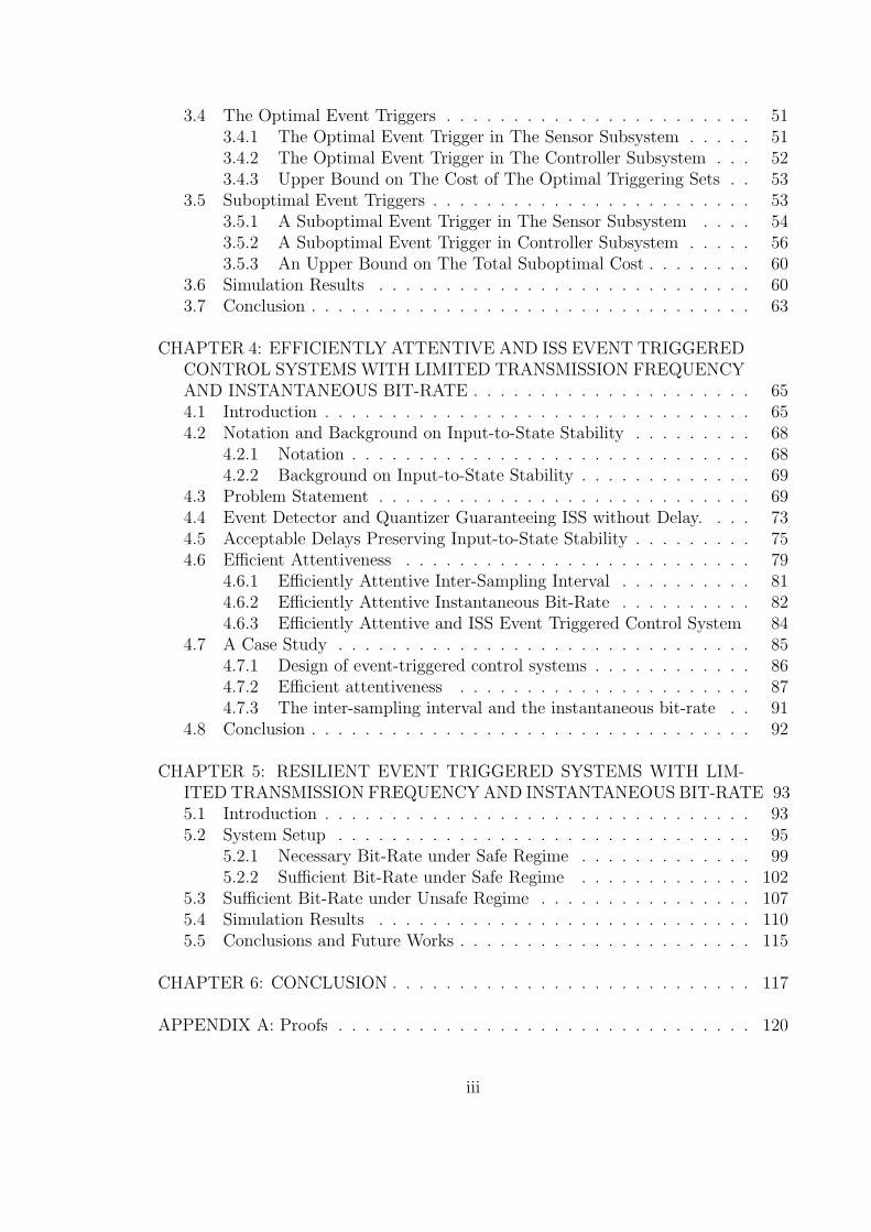
3.4 The Optimal Event Triggers . . . . . . . . . . . . . . . . . . . . . . . 513.4.1 The Optimal Event Trigger in The Sensor Subsystem . . . . . 513.4.2 The Optimal Event Trigger in The Controller Subsystem . . . 523.4.3 Upper Bound on The Cost of The Optimal Triggering Sets . . 53

3.5 Suboptimal Event Triggers . . . . . . . . . . . . . . . . . . . . . . . . 533.5.1 A Suboptimal Event Trigger in The Sensor Subsystem . . . . 543.5.2 A Suboptimal Event Trigger in Controller Subsystem . . . . . 563.5.3 An Upper Bound on The Total Suboptimal Cost . . . . . . . . 60

3.6 Simulation Results . . . . . . . . . . . . . . . . . . . . . . . . . . . . 603.7 Conclusion . . . . . . . . . . . . . . . . . . . . . . . . . . . . . . . . . 63

CHAPTER 4: EFFICIENTLY ATTENTIVE AND ISS EVENT TRIGGEREDCONTROL SYSTEMS WITH LIMITED TRANSMISSION FREQUENCYAND INSTANTANEOUS BIT-RATE . . . . . . . . . . . . . . . . . . . . . 654.1 Introduction . . . . . . . . . . . . . . . . . . . . . . . . . . . . . . . . 654.2 Notation and Background on Input-to-State Stability . . . . . . . . . 68

4.2.1 Notation . . . . . . . . . . . . . . . . . . . . . . . . . . . . . . 684.2.2 Background on Input-to-State Stability . . . . . . . . . . . . . 69

4.3 Problem Statement . . . . . . . . . . . . . . . . . . . . . . . . . . . . 694.4 Event Detector and Quantizer Guaranteeing ISS without Delay. . . . 734.5 Acceptable Delays Preserving Input-to-State Stability . . . . . . . . . 754.6 Efficient Attentiveness . . . . . . . . . . . . . . . . . . . . . . . . . . 79

4.6.1 Efficiently Attentive Inter-Sampling Interval . . . . . . . . . . 814.6.2 Efficiently Attentive Instantaneous Bit-Rate . . . . . . . . . . 824.6.3 Efficiently Attentive and ISS Event Triggered Control System 84

4.7 A Case Study . . . . . . . . . . . . . . . . . . . . . . . . . . . . . . . 854.7.1 Design of event-triggered control systems . . . . . . . . . . . . 864.7.2 Efficient attentiveness . . . . . . . . . . . . . . . . . . . . . . 874.7.3 The inter-sampling interval and the instantaneous bit-rate . . 91

4.8 Conclusion . . . . . . . . . . . . . . . . . . . . . . . . . . . . . . . . . 92

CHAPTER 5: RESILIENT EVENT TRIGGERED SYSTEMS WITH LIM-ITED TRANSMISSION FREQUENCYAND INSTANTANEOUS BIT-RATE 935.1 Introduction . . . . . . . . . . . . . . . . . . . . . . . . . . . . . . . . 935.2 System Setup . . . . . . . . . . . . . . . . . . . . . . . . . . . . . . . 95

5.2.1 Necessary Bit-Rate under Safe Regime . . . . . . . . . . . . . 995.2.2 Sufficient Bit-Rate under Safe Regime . . . . . . . . . . . . . 102

5.3 Sufficient Bit-Rate under Unsafe Regime . . . . . . . . . . . . . . . . 1075.4 Simulation Results . . . . . . . . . . . . . . . . . . . . . . . . . . . . 1105.5 Conclusions and Future Works . . . . . . . . . . . . . . . . . . . . . . 115

CHAPTER 6: CONCLUSION . . . . . . . . . . . . . . . . . . . . . . . . . . . 117

APPENDIX A: Proofs . . . . . . . . . . . . . . . . . . . . . . . . . . . . . . . 120

iii

BIBLIOGRAPHY . . . . . . . . . . . . . . . . . . . . . . . . . . . . . . . . . 123

iv

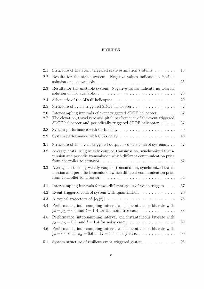
FIGURES

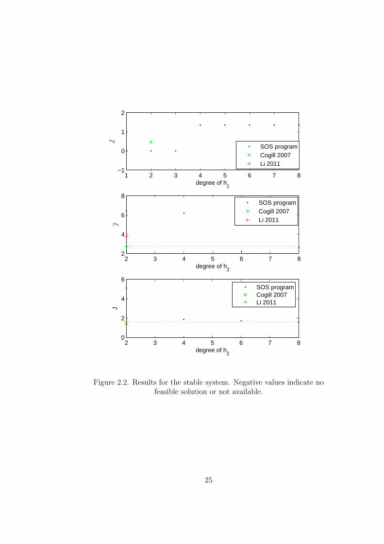
2.1 Structure of the event triggered state estimation systems . . . . . . . 15

2.2 Results for the stable system. Negative values indicate no feasiblesolution or not available. . . . . . . . . . . . . . . . . . . . . . . . . . 25

2.3 Results for the unstable system. Negative values indicate no feasiblesolution or not available. . . . . . . . . . . . . . . . . . . . . . . . . . 26

2.4 Schematic of the 3DOF helicopter. . . . . . . . . . . . . . . . . . . . 29

2.5 Structure of event triggered 3DOF helicopter . . . . . . . . . . . . . . 32

2.6 Inter-sampling intervals of event triggered 3DOF helicopter. . . . . . 372.7 The elevation, travel rate and pitch performance of the event triggered

3DOF helicopter and periodically triggered 3DOF helicopter. . . . . . 37

2.8 System performance with 0.01s delay . . . . . . . . . . . . . . . . . . 39

2.9 System performance with 0.02s delay . . . . . . . . . . . . . . . . . . 40

3.1 Structure of the event triggered output feedback control systems . . . 47

3.2 Average costs using weakly coupled transmission, synchronized trans-mission and periodic transmission which different communication pricefrom controller to actuator. . . . . . . . . . . . . . . . . . . . . . . . 62

3.3 Average costs using weakly coupled transmission, synchronized trans-mission and periodic transmission which different communication pricefrom controller to actuator. . . . . . . . . . . . . . . . . . . . . . . . 64

4.1 Inter-sampling intervals for two different types of event-triggers . . . 67

4.2 Event-triggered control system with quantization . . . . . . . . . . . 70

4.3 A typical trajectory of ∥ek(t)∥ . . . . . . . . . . . . . . . . . . . . . . 76

4.4 Performance, inter-sampling interval and instantaneous bit-rate withρθ = ρ∆ = 0.6 and l = 1, 4 for the noise free case. . . . . . . . . . . . 88

4.5 Performance, inter-sampling interval and instantaneous bit-rate withρθ = ρ∆ = 0.6, and l = 1, 4 for noisy case. . . . . . . . . . . . . . . . . 89

4.6 Performance, inter-sampling interval and instantaneous bit-rate withρθ = 0.6, 0.99, ρ∆ = 0.6 and l = 1 for noisy case. . . . . . . . . . . . . 90

5.1 System structure of resilient event triggered system . . . . . . . . . . 96

v

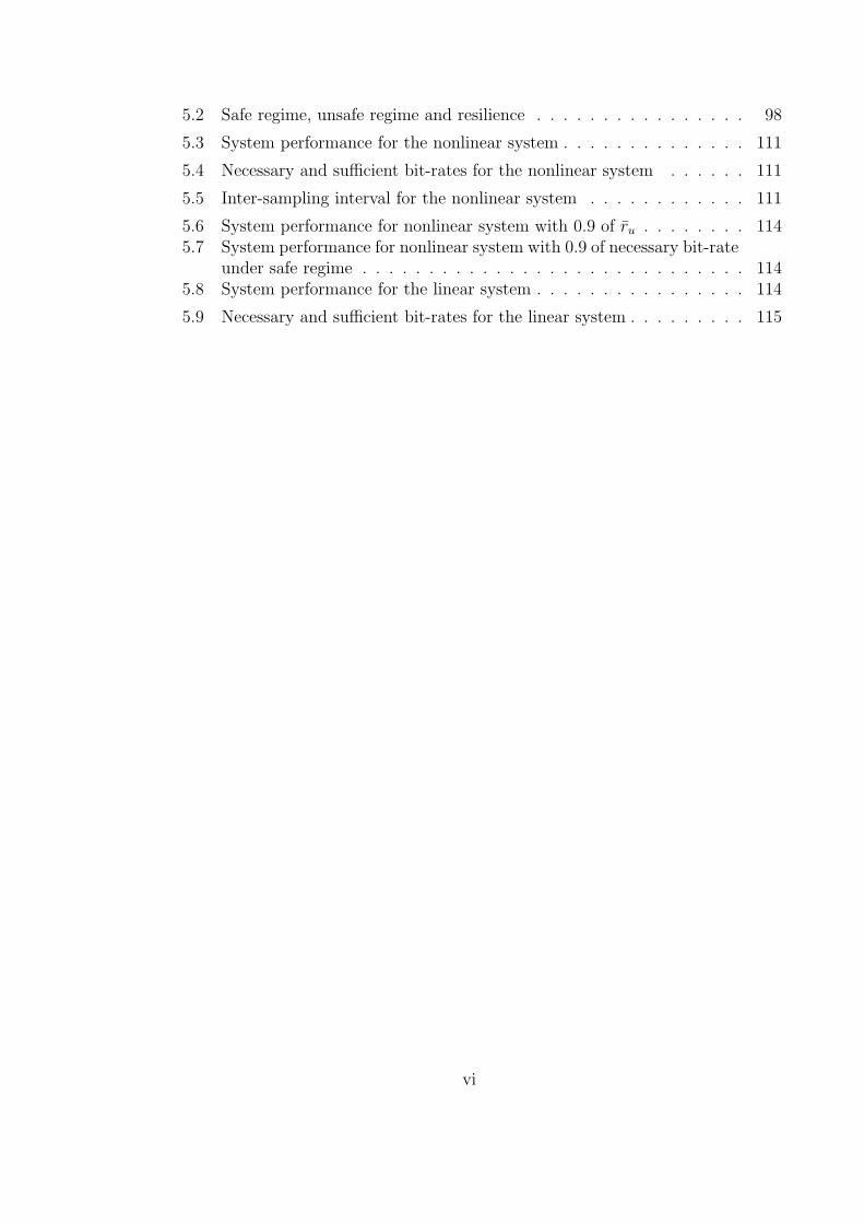
5.2 Safe regime, unsafe regime and resilience . . . . . . . . . . . . . . . . 98

5.3 System performance for the nonlinear system . . . . . . . . . . . . . . 111

5.4 Necessary and sufficient bit-rates for the nonlinear system . . . . . . 111

5.5 Inter-sampling interval for the nonlinear system . . . . . . . . . . . . 111

5.6 System performance for nonlinear system with 0.9 of ru . . . . . . . . 1145.7 System performance for nonlinear system with 0.9 of necessary bit-rate

under safe regime . . . . . . . . . . . . . . . . . . . . . . . . . . . . . 1145.8 System performance for the linear system . . . . . . . . . . . . . . . . 114

5.9 Necessary and sufficient bit-rates for the linear system . . . . . . . . . 115

vi

TABLES

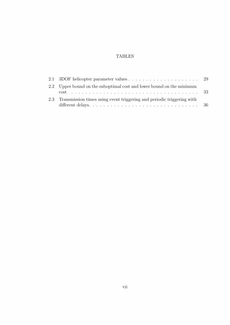
2.1 3DOF helicopter parameter values . . . . . . . . . . . . . . . . . . . . 29

2.2 Upper bound on the suboptimal cost and lower bound on the minimumcost . . . . . . . . . . . . . . . . . . . . . . . . . . . . . . . . . . . . 33

2.3 Transmission times using event triggering and periodic triggering withdifferent delays. . . . . . . . . . . . . . . . . . . . . . . . . . . . . . . 36

vii

CHAPTER 1

INTRODUCTION

The use of networking and information technology in control systems is making

our world smart. ‘Smart grid’ is expected to address the major challenges, such

as generation diversifications, demand response, energy conservation, environmental

compliance, and so on, of the existing electricity grid [28, 18]. ‘Smart manufactur-

ing system’ promises to reduce time-to-market, drive greater exports due to lower

production costs, and minimize energy use and materials while maximizing environ-

mental sustainability [58]. ‘Smart health-care system’ provides continuous monitoring

of patients, and minimizes the need of care-givers and helps the chronically ill and

elderly to survive an independent life [1]. ‘Smart farms’ optimally and sustainably

manage the water and land resources in agriculture [68].

While the integration of networking and information technology into control sys-

tems has the potential to reduce cost, increase operational efficiency, and promote

sustainability, there are two challenges in NIT-enabled control systems. The first

challenge is the limited transmission frequency. Many NIT-enabled control systems

make use of wireless sensor networks which usually has limited power [2, 10, 55]. Since

data transmission consumes significantly more energy than data processing [50], the

transmission frequency needs to be trimmed to prolong the network lifetime. The

second challenge is the limited instantaneous bit-rate. Networks, especially wireless

networks, have limited bandwidth, which means that there are only finite number of

bits in one packet, and this packet is transmitted with non-negligible delay. Since

both the limited transmission frequency and the limited instantaneous rate can dam-

1

age or degrade control systems [23], how to maintain system performance with limited

communication becomes a knotty problem.

To address this knotty problem, event triggered transmission was raised. Instead

of deciding the transmission times ahead of time as is done with periodic transmis-

sion, event triggered transmission uses on line information to detect the advent of

an event which triggers a transmission. There has been numerous experimental re-

sults to show shown that the event triggered transmission can significantly reduce

the transmission frequency while maintaining comparable system performance as

periodic transmission [5, 6, 59, 64, 15, 3, 44, 67, 63]. But little substantive work

analytically investigate the tradeoff between system performance and transmission

frequency, and the challenge of limited instantaneous bit-rate was totally ignored by

the prior work. Our research is to analytically examine the tradeoff among system

performance, transmission frequency, and instantaneous bit-rate in event triggered

state estimation and control systems.

One of the interesting questions about the tradeoff is what the best system per-

formance is for given limited transmission frequency. This question was first studied

in [29, 54] for minimum mean square state estimation error problem in finite horizon

during which only a finite number of transmissions were allowed. This problem was

treated as an optimal problem in a Markov decision process [53, 25], and the decision

to be made at each step is whether to transmit data. By dynamic programming, both

[29] and [54] showed that the optimal communication rule was event triggered. At

the same time, [70] explored the infinite horizon case. Instead of restricting the num-

ber of transmissions over a finite horizon, [70] assumed a cost for each transmission,

and studied the optimal stochastic communication rule which minimized the average

mean square state estimation error discounted by the transmission cost. In this case,

the decision to be made at each step is the probability of transmission. The optimal

communication rule was shown, again, to be event triggered.

2

The optimal event trigger, however, is difficult to compute because of the curse of

dimensionality in dynamic programming. So, computationally efficient suboptimal

event trigger is of interest. Most prior work approximated the value function with a

quadratic function or a set of quadratic functions, and then used the LMI toolbox

to efficiently compute the suboptimal event trigger [40, 35, 14, 12]. Although upper

bounds on the suboptimal cost were always provided, only [14] characterized how

far away its suboptimal cost was from the optimal cost by providing a lower bound

on the optimal cost. Even in this case, the lower bound on the optimal cost is only

effective for stable systems.

Instead of using quadratic functions, we used polynomials to approximate the

value functions, and provided computationally efficient suboptimal event trigger, an

upper bound on the suboptimal cost and a lower bound on the optimal cost [39, 37],

which will be presented in Chapter 2. These computationally efficient event trigger

and bounds on the costs are computed by searching for the solution of a set of linear

polynomial inequalities. The linear polynomial inequalities are transformed to a semi-

definite programming through the sum of squares decomposition of polynomials [11],

and hence efficiently solved. Our simulation results show that we can compute tighter

upper bounds on the suboptimal costs and tighter lower bounds on the optimal costs

than the prior work [14, 12, 35], while guaranteeing comparative actual costs as the

prior work [14, 12, 35].

After introducing the computationally efficient suboptimal event trigger for state

estimation problem, we will introduce computationally efficient suboptimal event

triggers for observer based output feedback control problem in Chapter 3 based on

our work in [36, 42]. The suboptimal event triggers are weakly coupled, which means

that the event trigger at the sensor and the event trigger at the controller are based

on local information only, the transmission at the sensor does not necessarily trigger

the transmission at the controller, and vice versa. This weakly coupled event trigger

3

design represents an advance over the recent work in event-triggered output feedback

control where transmission from the controller subsystem was tightly coupled to

the receipt of event-triggered sensor data [16], especially in multi-sensor networked

control systems.

All the work above only analyzes the tradeoff between system performance and

transmission frequency. The influence of limited instantaneous bit-rate is ignored. To

analyze the tradeoff among system performance, transmission frequency and instan-

taneous bit-rate, Chapter 4 and 5 explicitly consider not only inter-sampling interval,

but also quantization and network delay to achieve input-to-state stability (ISS) and

resilience, respectively.

Event triggered systems usually generate sporadic data packets. If properly

designed, longer inter-sampling interval and lower instantaneous bit-rate can be

achieved if the system state gets closer to the origin. This property is called efficient

attentiveness. Since for most of the time, the system state lies in a neighborhood of

its equilibrium, efficiently attentive event triggered systems only require infrequent

transmission and low instantaneous bit-rate to maintain system performance. Effi-

cient attentiveness, however, is not a necessary property of event triggered systems,

a counter example was provided in [38].

Chapter 4 concludes our research in [66, 41, 43], provides a sufficient condition to

guarantee efficient attentiveness, and obtains the minimum inter-sampling interval

and a sufficient instantaneous bit-rate to guarantee ISS. Quantization error and the

acceptable delay that preserving ISS are explicitly studied. Different from the prior

work which considered constant bounded delay [71, 72, 20, 33], the acceptable delay

we present is state dependent. In our simulation, the required instantaneous bit-

rate increases sharply as the inter-sampling interval increases. This fact indicates

that with limited bandwidth, we should not only focus on lengthening inter-sampling

interval, but also need to guarantee that the channel bandwidth satisfies the required

4

instantaneous bit-rate.

Efficiently attentive event triggered systems can have long inter-sampling interval

when the system state is close to its equilibrium. A prime concern about this long

inter-sampling interval is whether event triggered control systems are resilient to

unexpected disturbances which appear between two consecutive transmissions. By

‘resilience’, we mean that the system’s ability to return to its operational normalcy

in the presence of unexpected disturbances.

Chapter 5 addresses the resilience issue in an event triggered scalar nonlinear

system with transient unknown magnitude disturbances. When the system is in

normal situation, a necessary instantaneous bit-rate and a sufficient instantaneous

bit-rate are given to assure uniform boundedness. If the system was linear, it was

shown that the sufficient bit-rate achieves the necessary bit-rate. When the system is

hit by transient unknown magnitude disturbances, a sufficient instantaneous bit-rate

is provided to guarantee resilience, i.e. return to a neighborhood of the origin in a

finite time.

5

CHAPTER 2

MINIMUM MEAN SQUARE STATE ESTIMATION ERROR WITH LIMITED

TRANSMISSION FREQUENCY

2.1 Introduction

Because of the very limited bandwidth in wireless channels, most wireless net-

worked control systems have communication constraints, especially when the sensors

are battery driven. Since wireless communication is a major source of power consump-

tion [55, 57, 2], efficient management of wireless communication is very important to

extend the working life of the whole wireless networked control systems.

To efficiently manage the wireless communication, some prior work [30, 54] searched

for the optimal communication rule which minimized the mean square state estima-

tion error under the communication constraint that only a limited number of trans-

missions were allowed in a finite horizon. The optimal communication rule was shown

to be event triggered. Under Event triggered communication rule, transmission oc-

curs only if some event occurs. Prior work in [5, 6, 59, 64, 45, 3, 24, 15] has shown

the advantage of event triggered communication over periodic communication on re-

ducing transmission frequency while maintaining system performance. The optimal

event trigger, however, is computationally complicated. This computational complex-

ity limited [30] and [54] to scalar cases. At the same time, [70] studied the optimal

communication rule which minimized the average mean square state estimation error

discounted by the transmission cost in infinite horizon. The optimal communication

rule was still event triggered, and difficult to compute.

6

Because of the computational complexity of the optimal event trigger, computa-

tionally efficient suboptimal event triggers are of interest. For finite horizon cases,

[40] provided a quadratic suboptimal event trigger which involved backward recur-

sive matrix multiplication. For infinite horizon cases, [14] also provided a quadratic

suboptimal event trigger, but this quadratic suboptimal event trigger was only for

stable systems. Later, [12] and [35] presented suboptimal event triggers for both

stable and unstable systems based on linear matrix inequalities (LMI). Although all

these prior work [40, 14, 12, 35] gave upper bounds on their suboptimal costs, only

[14] characterized how far away its suboptimal cost was from the optimal cost by

giving a lower bound on the optimal cost, and this lower bound was only effective in

stable systems.

This chapter presents not only computationally efficient suboptimal event trigger

and an upper bound on its cost, but also computationally efficient lower bound on

the optimal cost. All of them are effective for both stable and unstable systems, and

computed based on linear polynomial inequalities. Linear polynomial inequalities

can be transformed to a semi-definite programming (SDP) based on sums of squares

(SOS) decomposition of polynomials through SOSTOOLS [52], and hence efficiently

solved by SeDuMi [8] or SDPT3 [62]. Our simulation results show that we can

compute tighter upper bounds on the suboptimal costs and tighter lower bounds on

the optimal costs than the prior work [14, 12, 35], while guaranteeing comparative

actual costs as the prior work [14, 12, 35].

Later, we apply the polynomial event triggers to an 8 dimensional 3 degree of free-

dom (3DOF) helicopter. To our best knowledge, this is the first time the suboptimal

event trigger has been applied to a system whose dimension is greater than 2. Our

simulation results show that with polynomial event triggers, the 3DOF helicopter

tracked the reference signal with small overshoot and no steady error. This event

triggered helicopter used less communication resource than periodically triggered he-

7

licopter with comparable performance, and bore the same amount of transmission

delay as the periodically triggered helicopter while maintaining the system perfor-

mance.

2.2 Background on Average Optimality for Markov Control Processes

This section presents the existing work on average optimality for Markov control

processes, since this existing work is the basis for the main results in this chapter.

A Markov control process, which is also called Markov decision process [? ]

or controlled Markov process [17], is a stochastic dynamical system specified by the

five-tuple [4, 25]

X,A, A(x)|x ∈ X, Q(·|x ∈ X, a ∈ A), c , (2.1)

where

• X is a Borel space (e.g. Rn, finite set, and countable set), called the state space;

• A is a Borel space, called the action space;

• A(x) is a non-empty measurable subset of A, denoting the set of all feasibleactions when the system is in state x ∈ X. Suppose that the set of feasiblestate-action pairs

K = (x, a)|x ∈ X, a ∈ A(x)

is also a Borel space;

• Q is a conditional probability function on X given K, called the transitionlaw. Let D be a Borel set of X, and x(t), t ∈ N0 and a(t), t ∈ N0 bestochastic processes. Q(D|x(t), a(t)) = P (x(t + 1) ∈ D|x(t), a(t)), where P isthe cumulative probability function.

• c : K → R is the (measurable) one-stage cost function.

Given a Markov control process described as above, an action at step t is decided

based on all the history state and action information. Let H(t) denote the admissible

8

history up to time t. It is defined as

H(0) = X,H(t+ 1) = H(t)×K, ∀t ∈ N0.

An element h(t) of H(t) is a vector of the form

h(t) = (x(0), a(0), . . . , x(t− 1), a(t− 1), x(t)).

An admissible control strategy or policy is a sequence π = π(·, t|·), t ∈ N0

of stochastic kernel π(t) on the action space A given H(t) satisfying the constraint

π(A(x(t)), t|h(t)) = 1,∀h(t) ∈ H(t), t ∈ N0. (2.2)

The set of all policies is denoted by Π.

Generally, the action a(t) is a random variable in action space A. π(·, t|h(t))

characterize the probability distribution of a(t) given h(t). Equation (2.2) indicates

that all possible actions produced by an (admissible) policy π are in the feasible

action set A(x(t)).

A specific case is that A policy becomes deterministic and stationary. A policy π

is said to be a deterministic stationary policy if there is a function f : X → A

with f(x) ∈ A(x) for all x ∈ X such that

π(f(x(t)), t|h(t)) = π(f(x(t))|x(t)) = 1, ∀h(t) ∈ H(t),∀t ∈ N0.

f is said to be a deterministic stationary rule.

Given a Markov control process and a policy π, the expected long-run average

9

cost incurred by π is given by

V (π, x) = lim supN→∞

E

[1

N

N−1∑t=0

c(x(t), a(t))

],

where a(t) is the action taken at step t, and the average optimal value function V ∗(x)

is as follows:

V ∗(x) = infπ∈Π

V (π, x).

First, we state the conditions for the existence of an average optimal deterministic

stationary policy. The first condition is a Lyapunov-like condition.

Assumption 2.2.1 (Lyapunov-like condition). 1. There exist constants b > 0and β ∈ (0, 1), and a (measurable) function ω(x) ≥ 1 for all x ∈ X such that∫

X

ω(y)Q(dy|x, a) ≤ βω(x) + b, ∀(x, a) ∈ K.

2. There exists a constant M > 0, such that |c(x, a)| ≤ Mω(x) for all (x, a) ∈ K.

The second condition is a continuity condition on the action space.

Assumption 2.2.2 (Continuity condition on action space). For any state x ∈

X,

1. The feasible action set A(x) is compact.

2. The one-state cost function c(x, a) is lower semi-continuous in a ∈ A(x);

3. The function a 7→∫Xυ(y)Q(dy|x, a) is continuous on A(x) for all bounded mea-

surable functions υ on X.

Remark 2.2.3. Assumption 2.2.2 holds when A(x) is finite for all x ∈ X.

For the function ω > 1 in Assumption 2.2.1, let us first define a Banach space

10

Bω(X) as

Bω(X) = ν : supx∈X

ω(x)−1|ν(x)| < ∞.

The third condition is a uniform boundedness condition on parameter α which is

described as the following.

Assumption 2.2.4 (Uniform boundedness condition w.r.t. α). There exist

two functions ν1, ν2 ∈ Bω(X), and some state x0 ∈ X, such that

ν1(x) ≤ hα(x) ≤ ν2(x), ∀x ∈ X,∀α ∈ (0, 1),

where hα(x) = V ∗α (x)− V ∗

α (x0), and V ∗α (x) = mina∈A(x)E [

∑∞t=0 α

tc(x(t), a(t))] is the

minimum discounted cost satisfying

V ∗α (x) = min

a∈A(x)

c(x, a) + α

∫X

V ∗α (y)Q(dy|x, a)

, (2.3)

for all x ∈ X.

We now give the main results about average optimality. Please check Theorem

4.1 of [22] for the proofs of Lemma 2.2.5 and Corollary 2.2.6 and 2.2.7.

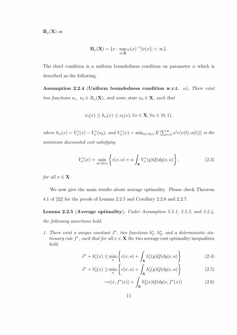
Lemma 2.2.5 (Average optimality). Under Assumption 2.2.1, 2.2.2, and 2.2.4,

the following assertions hold.

1. There exist a unique constant J∗, two functions h∗1, h

∗2, and a deterministic sta-

tionary rule f∗, such that for all x ∈ X the two average cost optimality inequalitieshold.

J∗ + h∗1(x) ≤min

a

c(x, a) +

∫X

h∗1(y)Q(dy|x, a)

(2.4)

J∗ + h∗2(x) ≥min

a

c(x, a) +

∫X

h∗2(y)Q(dy|x, a)

(2.5)

=c(x, f ∗(x)) +

∫X

h∗2(x)Q(dy|x, f ∗(x)) (2.6)

11

2. J∗ = V ∗(x) for all x ∈ X.

3. Any deterministic stationary rule f realizing the minimum of (2.5) is averageoptimal; thus, f ∗ in (2.6) is a deterministic stationary policy for the average costproblem.

Corollary 2.2.6 (Lower bounds on optimal costs). Under Assumption 2.2.1,

2.2.2, and 2.2.4, the following assertions hold.

1. There exist a constant J and a function h1, such that for all x ∈ X

J + h1(x) ≤ mina∈A(x)

c(x, a) +

∫X

h1(y)Q(dy|x, a).

2. J∗ ≥ J .

Corollary 2.2.7 (Suboptimal event triggers and the corresponding upper

bounds). Under Assumption 2.2.1, 2.2.2, and 2.2.4, the following assertions hold.

1. There exist a constant J , a function h2, and a deterministic stationary rule f ,such that for all x ∈ X

J + h2(x) ≥ mina∈A(x)

c(x, a) +

∫X

h2(x)Q(dy|x, a)

=c(x, f(x)) +

∫X

h2(x)Q(dy|x, f(x)).

2. V (f, x) ≤ J .

Remark 2.2.8. Similar results to that of Corollary 2.2.6 and 2.2.7 can also be found

in [13].

2.3 Background on SOSTOOLS

Our suboptimal event triggers are computed based on the solution of a set of

polynomial inequalities. Since SOSTOOLS automatically transforms polynomial in-

equalities to a semi-definite program (SDP) based on the sums of squares decom-

position (SOS) of polynomials, we can use SOSTOOLS to efficiently compute the

12

suboptimal event trigger. In this section, we presents a brief review of the basic idea

of SOSTOOLS.

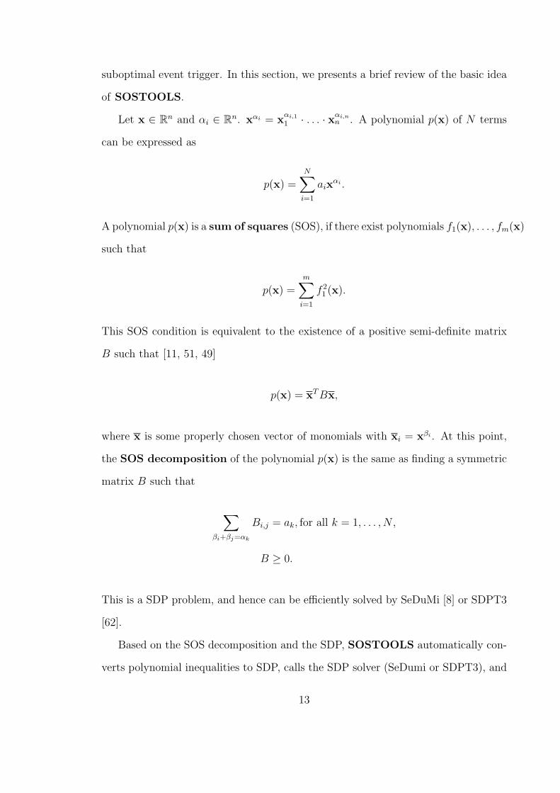
Let x ∈ Rn and αi ∈ Rn. xαi = xαi,1

1 · . . . · xαi,nn . A polynomial p(x) of N terms

can be expressed as

p(x) =N∑i=1

aixαi .

A polynomial p(x) is a sum of squares (SOS), if there exist polynomials f1(x), . . . , fm(x)

such that

p(x) =m∑i=1

f 21 (x).

This SOS condition is equivalent to the existence of a positive semi-definite matrix

B such that [11, 51, 49]

p(x) = xTBx,

where x is some properly chosen vector of monomials with xi = xβi . At this point,

the SOS decomposition of the polynomial p(x) is the same as finding a symmetric

matrix B such that

∑βi+βj=αk

Bi,j = ak, for all k = 1, . . . , N ,

B ≥ 0.

This is a SDP problem, and hence can be efficiently solved by SeDuMi [8] or SDPT3

[62].

Based on the SOS decomposition and the SDP, SOSTOOLS automatically con-

verts polynomial inequalities to SDP, calls the SDP solver (SeDumi or SDPT3), and

13

converts the SDP solution back to the solution of the original polynomial inequal-

ities. The basic feasibility problem that the SOSTOOLS solves is formulated as

finding polynomials pi(x) for i = 1, 2, . . . , N , such that

a0,j(x) +N∑i=1

pi(x)ai,j(x) = 0, for j = 1, 2, . . . , J (2.7)

a0,j(x) +N∑i=1

pi(x)ai,j(x) ≥ 0, for j = J + 1, . . . , J , (2.8)

where ai,j(x) are given scalar constant coefficient polynomials.

SOSTOOLS also solves the problem of optimizing of an objective function which

is linear in the coefficients of pi(x)’s. This optimization problem is formulated as

searching for pi(x) for i = 1, 2, . . . , N that

minc

wT c (2.9)

subject to: equation (2.7) and (2.8),

where w is a given weight vector, and c is a vector consisting of the coefficients of

pi(x)’s.

To define and solve an SOS programming using SOSTOOLS, please check Chapter

2 of [52].

2.4 Event Triggered State Estimation problem

Consider a state estimation system shown in Figure 2.1. The plant is a discrete

time, linear, time invariant system described by the following difference equation.

x(k) = Ax(k − 1) + w(k − 1),

y(k) = Cx(k) + v(k), for k = 1, 2, . . . ,∞.

14

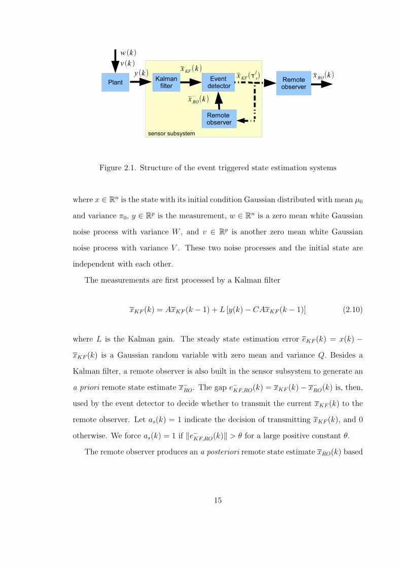
Figure 2.1. Structure of the event triggered state estimation systems

where x ∈ Rn is the state with its initial condition Gaussian distributed with mean µ0

and variance π0, y ∈ Rp is the measurement, w ∈ Rn is a zero mean white Gaussian

noise process with variance W , and v ∈ Rp is another zero mean white Gaussian

noise process with variance V . These two noise processes and the initial state are

independent with each other.

The measurements are first processed by a Kalman filter

xKF (k) = AxKF (k − 1) + L [y(k)− CAxKF (k − 1)] (2.10)

where L is the Kalman gain. The steady state estimation error eKF (k) = x(k) −

xKF (k) is a Gaussian random variable with zero mean and variance Q. Besides a

Kalman filter, a remote observer is also built in the sensor subsystem to generate an

a priori remote state estimate x−RO. The gap e−KF,RO(k) = xKF (k)− x−

RO(k) is, then,

used by the event detector to decide whether to transmit the current xKF (k) to the

remote observer. Let as(k) = 1 indicate the decision of transmitting xKF (k), and 0

otherwise. We force as(k) = 1 if ∥e−KF,RO(k)∥ > θ for a large positive constant θ.

The remote observer produces an a posteriori remote state estimate xRO(k) based

15

on the following difference equation.

x−RO(k) =AxRO(k − 1), (2.11)

xRO(k) =

x−RO(k), if as(k) = 0;

xKF (k), if as(k) = 1 ,(2.12)

Let us define the remote state estimation error eRO(k) as

eRO(k) = x(k)− xRO(k).

The average cost in this event triggered state estimation problem is

J(as(k)∞k=0) = limN→∞

1

N

N−1∑k=0

E (c(eRO(k), as(k))) , (2.13)

where the cost function

c(eRO(k), as(k)) = ∥eRO(k)∥2Z + as(k)λ, (2.14)

∥eRO(k)∥2Z = eRO(k)TZeRO(k) with a given semi-positive definite n × n matrix Z,

and λ is the communication price for one transmission.

Noticing that eKF,RO(k) is orthogonal to the filtered state error eKF (k) (please

check Lemma A.0.1 in Appendix A for the proof), together with the dynamic behavior

of xKF and x−RO, the average cost is rewritten as

J(as(k)∞k=0) = limN→∞

1

N

N−1∑k=0

E(cn(e

−KF,RO(k), as(k))

)+ trace(QZ),

16

where

cn(e−KF,RO(k), as(k)) = as(k)λ+ (1− as(k))∥e−KF,RO(k)∥

2Z .

Our objective is to find a transmission rule to minimize the average cost J(as(k)∞k=0),

i.e.

J∗ = minas(k)∞k=0

J(as(k)∞k=0). (2.15)

2.5 The Optimal Event Trigger

This optimal problem was solved in [70], but the optimal solution is difficult to

compute. For the completeness of this paper, we state the optimal solution in [70]

without proof.

Theorem 2.5.1. Let

Th(s, l) = E(h(e−KF,RO(k + 1))|e−KF,RO(k) = s, as(k) = l

),

where s ∈ Rn and l ∈ 0, 1.

1. There exist a unique constant ρ∗ and a function h∗, such that for all s ∈ Rn

ρ∗ + h∗(s) =min∥s∥2Z + Th∗ (s, 0) , λ+ Th∗ (s, 1)

, (2.16)

2. The optimal cost J∗ = ρ∗ + trace(QZ).

3. The optimal event trigger is

a∗s(k) =

1, if V0(e

−KF,RO(k)) ≥ V1(e

−KF,RO(k)) or ∥e−KF,RO(k)∥ > θ,

0, otherwise.

where V0(s) = ∥s∥2Z + Th∗ (s, 0) , and V1(s) = λ+ Th∗ (s, 1) .

Remark 2.5.2. It is hard to find a solution to equation (2.16). Although we can

iteratively compute the solution of equation (2.16) by value iteration [21] or policy

17

iteration [47, 26], the computational complexity increases exponentially with respect

to the state dimension.

2.6 A Computationally Efficient Lower Bound on The Optimal Cost

Although the optimal cost is difficult to compute, we can efficiently compute a

lower bound on the optimal cost based on SOSTOOLS. This section first gives a

theorem about the lower bound on the optimal cost, and then discusses how to use

SOSTOOLS to compute the largest lower bound on the optimal cost.

Theorem 2.6.1. If there exists a constant ρ1 and a polynomial function h1, such

that for all s ∈ Rn

ρ1 + h1(s) ≤∥s∥2Z + Th1 (s, 0) , (2.17)

ρ1 + h1(s) ≤λ+ Th1(s, 1), (2.18)

then J∗ ≥ J∗ = ρ1 + trace(QZ).

Proof. Equation (2.17) and (2.18) indicate that

ρ1 + h1(e−KF,RO(k))

≤ minas(k)∈0,1

cn(e−KF,RO(k), as(k)) + Th1(e

−KF,RO(k), as(k))

≤cn(e−KF,RO(k), as(k)) + Th1(e

−KF,RO(k), as(k))

The expected values of both sides of the above inequality satisfy

ρ1 + E(h1(e−KF,RO(k)))

≤E(cn(e−KF,RO(k), as(k))) + E(h1(e

−KF,RO(k + 1))).

Varying k from 0 to N , and adding all these inequalities together, we have, for all

18

feasible as(k)Nk=0,

ρ1 ≤∑N

k=0 E(cn(e−KF,RO(k), as(k)))

N(2.19)

+E(h1(e

−KF,RO(N + 1)))− E(h1(e

−KF,RO(0)))

N.

Since as(k) is forced to be 1 if ∥e−KF,RO(k)∥ > θ, from equation (2.11) and (2.12),

it is easy to see that

∥e−KF,RO(k)∥ ≤ θ, for all k = 0, 1, · · · .

Since h1 is a polynomial, we know that E(h1(e−KF,RO(k))) < ∞ for all k = 0, 1, · · · ,

and

ρ1 ≤ limN→∞

1

N

N∑k=0

E(cn(e−KF,RO(k), as(k))),

for all feasible as(k)∞k=0.

Therefore, ρ1 + traceQZ ≤ J∗.

Remark 2.6.2. Equation (2.17) and (2.18) are polynomial inequalities whose coeffi-

cients are linear combinations of the coefficients of h1. It is easy to get the dynamic

behavior of e−KF,RO from equation (3.2), (2.11) and (2.12) as the following.

e−KF,RO(k + 1) = (1− as(k))Ae−KF,RO(k) + Ly(k) (2.20)

where y(k) = CAeKF (k)+Cw(k)+v(k+1) is a zero mean Gaussian random variable

with covariance Y = CAQATCT + CWCT + V .

Therefore, Th1 (s, 0) = E(h1(s′)) where s′ is a Gaussian random variable with

mean As and covariance Y , and Th1 (s, 1) = E(h1(s′)) where s′ is a zero mean Gaus-

sian random variable with covariance Y .

19

According to the Isserlis’ theorem 1, Th1 (s, 0) and Th1 (s, 1) are polynomials whose

coefficients are linear combinations of the coefficients of h1.

So, Equation (2.17) and (2.18) are both polynomial inequalities whose coefficients

are linear combinations of the coefficients of h1.

Remark 2.6.3. Since equation (2.17) and (2.18) are polynomial inequalities whose

coefficients are linear combinations of the coefficients of h1, the largest lower bound

on the optimal cost can be efficiently computed by the following SOS programming.

min−ρ1 (2.21)

subject to: (2.17) and (2.18)

2.7 A Computationally Efficient Suboptimal Event Trigger

The last section talks about how to compute the largest lower bound on the

optimal cost based on SOSTOOLS, but does not provide a computationally effective

suboptimal event trigger. In this section, a suboptimal event trigger and an upper

bound on its cost are provided, and an SOS based algorithm is given to efficiently

search for the smallest upper bound on the suboptimal cost.

Theorem 2.7.1. Let sϕ = [sϕ1 sϕ2 . . . sϕn]T , where s ∈ Rn and ϕ is a positive integer.

Given a positive constant d, and positive integers ϕ and δ, if there exist a constant

ρ2, and a positive definite polynomial function h2 such that the following inequalities

1[Isserlis’ theorem:] If (x1, . . . , x2n) is a zero mean multivariate normal random vector, then

E(x1x2 · · · , x2n) =∑∏

E(xixj),

E(x1x2 · · · , x2n−1) =0,

where the notation∑∏

means summing over all distinct ways of partitioning x1, . . . , x2n into pairs.[31]

20

hold for all s ∈ Rn,

(∥s∥2z + Th2(s, 0))

(1− ∥sϕ∥2Z − d

500d

)≤ρ2 + h2(s) (2.22)

(λ+ Th2(s, 1))(∥sϕ∥2Z + ∥sϕ+δ∥2Z) ≤(ρ2 + h2(s))(d+ ∥sϕ+δ∥2Z) (2.23)

then there exists a suboptimal event trigger

as,2(k) =

1, if V0(e−KF,RO(k)) ≥ V1(e

−KF,RO(k)) or ∥e−KF,RO(k)∥ > θ,

0, otherwise.

where V0(s) = ∥s∥2Z + Th2 (s, 0) , and V1(s) = λ + Th2 (s, 1) , and the suboptimal cost

satisfies

J(as,2(k)∞k=0) ≤ J = ρ2 + trace(QZ).

Proof. Rewrite equation (2.23) as

(λ+ Th2(s, 1))

(1 +

∥sϕ∥2Z − d

d+ ∥sϕ+δ∥2Z

)≤ρ2 + h2(s). (2.24)

It is easy to find that no matter whether ∥sϕ∥2Z − d ≥ 0 is true, equation (2.22) and

(2.24) indicate that

ρ2 + h2(s) ≥minas(k)

V0(s), V1(s)

=cn(s, as,2(k)) + Th2(s, as,2(k))

Following the same steps in the proof of Theorem 2.6.1, we have

ρ2 ≥ limN→∞

1

N

N∑k=0

E(cn(e−KF,RO(k), as,2(k))),

and J(as,2(k)∞k=0) ≤ ρ2 + trace(QZ).

21

Remark 2.7.2. Equation (2.22) and (2.23) are polynomial inequalities whose co-

efficients are linear combinations of the coefficients of h2. From Remark 2.6.2, we

know that Th2(s, 0) and Th2(s, 1) are both polynomials whose coefficients are linear

combinations of the the coefficients of h2. Since 1 − ∥sϕ∥2Z−d

500d, ∥sϕ∥2Z + ∥sϕ+δ∥2Z, and

d+∥sϕ+δ∥2Z are all given constant coefficient polynomials, equation (2.22) and (2.23)

are polynomial inequalities whose coefficients are linear combinations of the coeffi-

cients of h2.

Remark 2.7.3. Since equation (2.22) and (2.23) are polynomial inequalities whose

coefficients are linear combinations of the coefficients of h2, h2 and ρ2, as,2 and J can

be efficiently computed using SOSTOOLS by solving the following SOS programming.

min ρ2 (2.25)

subject to: (2.22) and (2.23).

Remark 2.7.4. The degree, ϕ and δ, of the constant coefficient polynomials 1 −∥sϕ∥2Z−d

500d, ∥sϕ∥2Z + ∥sϕ+δ∥2Z, and d + ∥sϕ+δ∥2Z should be chosen as large as possible as

long as the computation time is not too long. Generally speaking, higher ϕ and δ

can provide smaller ρ2 for h2 with the same degree, but consumes more computation

effort. So, ϕ and δ can be chosen to be large enough such that the computation time

is not too long.

Remark 2.7.5. The positive scalar constant, d, in the constant coefficient polyno-

mials 1− ∥sϕ∥2Z−d

500dand d+ ∥sϕ+δ∥2Z is chosen through Lipschitz optimization such that

ρ2 computed according to equation (2.25) is minimized. Built upon Lipschitz opti-

mization, DIRECT algorithm [19] is a matlab based function which is used in our

algorithm to search for the scalar constant d∗ which provides the smallest ρ2.

Algorithm 2.7.6 (Compute the suboptimal event trigger).

22

1. Initialization

i Provide system parameters: A, C, W , V , L, Q, Z, and λ.

ii Provide parameters in equation (2.22) and (2.23): ϕ, δ.

iii Initialize an SOS programming using toolbox ‘SOSTOOLS’.

• Declare scalar decision variables: ρ2, s1, . . . , sn (s = [s1, . . . , sn]T de-

notes e−KF,RO(k) in equation (2.22) and (2.23)).

• Declare a polynomial variable: h2.

• Compute Th2(s, 0) and Th2(s, 1) using the Isserlis’ theorem.

2. Use DIRECT function to search interval [0, 5λ] for the d∗ which provides thesmallest ρ2.

3. Solve the SOS programming (2.25) with d = d∗.

4. Compute the suboptimal event trigger: sTZs+ Eh2(As)− λ− Eh2(0) > 0.

5. Compute the upper bound on the suboptimal cost: ρ2 + trace(QZ).

6. Return.

2.8 Mathematical Examples

The last two sections propose SOS programs to efficiently compute a lower bound

on the optimal cost, and a suboptimal event trigger and an upper bound on its cost.

This section will use two examples to show that SOS program (2.21) and (2.25) can

compute tighter lower bound on the optimal cost and tighter upper bound on the

suboptimal cost than the prior work [14, 12, 35], while guaranteeing almost the same

actual cost as the prior work [14, 12, 35].

23

2.8.1 Stable system

Consider a marginally stable system as below

x(k + 1) =

1 0

0 1

x(k) + w(k)

y(k) =x(k),

with covariance matrix W =

0.03 −0.02

−0.02 0.04

, the weight matrix Z =

2 1

1 2

,and the communication price λ = 20. This is the same example used in [14], and we

would like to compare our results with the results in [14] and [35].

The SOS program (2.21) was first used to compute a lower bound J on the

minimum cost. In this program, h1 was set to be a polynomial which contained all

possible monomials whose degrees were no greater than D1. We varied D1 from 1 to

8, and the computed largest lower bounds are shown in the top plot of Figure 2.2.

We find when the degree of h1 was increased to be 4, the lower bound provided by

the SOS program (2.21) was larger than the lower bound provided by [14] by about

2 times, while [35] did not talk about how to compute a lower bound on the optimal

cost.

We, then, use SOS program (2.25) to compute a suboptimal event trigger and

an upper bound on its cost. In this program, h2 was set to be a polynomial which

contained all possible monomials whose degrees were even and no greater than D2.

let ϕ = 3 and δ = 1. The constant d is chosen using the DIRECT optimization

algorithm. The degree of h2, D2, was varied from 1 to 8, and the computed upper

bounds on the suboptimal cost are shown in the middle plot of Figure 2.2. We see

that when the degree of h2 was increased to 6, the upper bound on the suboptimal

cost was smaller than the upper bounds provided by [14] and [35].

24

1 2 3 4 5 6 7 8−1

0

1

2

degree of h1

J

SOS programCogill 2007Li 2011

2 3 4 5 6 7 82

4

6

8

degree of h2

J


2 3 4 5 6 7 80

2

4

6

degree of h2

J


Figure 2.2. Results for the stable system. Negative values indicate nofeasible solution or not available.

25

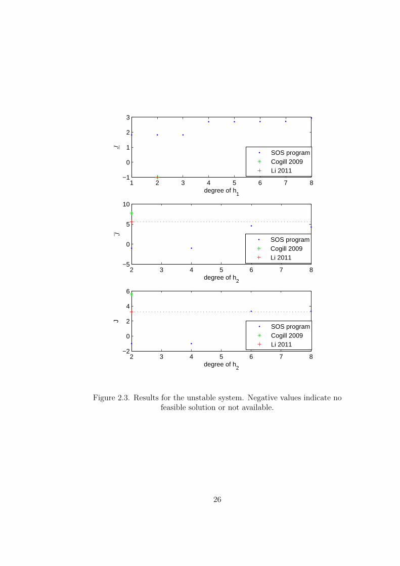
1 2 3 4 5 6 7 8−1

0

1

2

3

degree of h1

J


2 3 4 5 6 7 8−5

0

5

10

degree of h2

J


2 3 4 5 6 7 8−2

0

2

4

6

degree of h2

J


Figure 2.3. Results for the unstable system. Negative values indicate nofeasible solution or not available.

26

The suboptimal event triggers were, then, used in the state estimation system,

and the actual costs are given in the bottom plot of Figure 2.2. We find that when

the degree of h2 was increased to 6, the actual cost is almost the same as the actual

costs provided by [14] and [35].

2.8.2 Unstable system

Next, we consider an unstable system.

x(k + 1) =

0.95 1

0 1.01

x(k) + w(k)

y(k) =

[0.1 1

]x(k) + v,

with the covariance matrix W =

0.2 0

0 0.2

and V = 0.3, the weight matrix

Z =

1 0

0 1

, and the communication price λ = 5.

With the same steps as we did for the stable system, we computed the lower bound

J on the minimum cost while varying the degree of h1 from 1 to 8. The results are

given in the top plot of Figure 2.3. We see that when the degree of h1 is greater than

4, the lower bound on the optimal cost is always greater than 2.7, while there is no

prior work provided lower bounds on the optimal cost for unstable systems.

Follow the same steps as what we did for the stable system, we computed the

suboptimal event trigger, and the upper bound J on its cost. In this case, the degree

ϕ and δ in equation (2.22) and (2.23) is set to be 6 and 1, respectively. We varied the

degree of h2 from 2 to 8, the upper bounds on the suboptimal costs are given in the

middle plot of Figure 2.3. We see that when the degree of h2 was increased to 6, the

upper bounds on the suboptimal costs are smaller than the upper bounds provided

27

by both [12] and [35].

The suboptimal event triggers were, then, applied to the state estimation system.

The actual costs are shown in the bottom plot of Figure 2.3. We see that when the

degree of h2 is greater than 6, the actual costs are almost the same as the actual cost

given by [35], and are less than the actual cost provided by [12].

2.9 Application in a QUANSER c⃝ 3DOF Helicopter

This section applies the suboptimal event trigger computed from Algorithm 2.7.6

to a 8 dimensional nonlinear 3DOF helicopter. Subsection 2.9.1 introduces the non-

linear model of the 3DOF helicopter, linearization of this nonlinear model and the

controllers we will use for the 3DOF helicopter. Subsection 2.9.2 explains how we de-

sign the suboptimal event triggers for this 3DOF helicopter. The experiment results

are given in subsection 2.9.3.

2.9.1 QUANSER c⃝ 3DOF Helicopter

Figure 2.4 gives the basic schematic of the 3DOF helicopter. The 3DOF helicopter

consists of three subsystems: elevation (ϵ), pitch (ρ) and travel (γ). Elevation is the

angle between the main beam and the horizontal axis, pitch is the angle that the

motor beam moves around the main beam, and travel is the angle that the main

beam moves around the vertical axis. Tf and Tb are the front and back thrusts

generated by the DC motors. Our objective is to control the 3DOF helicopter to

follow a commanded elevation ϵr and a commanded travel rate γr.

28

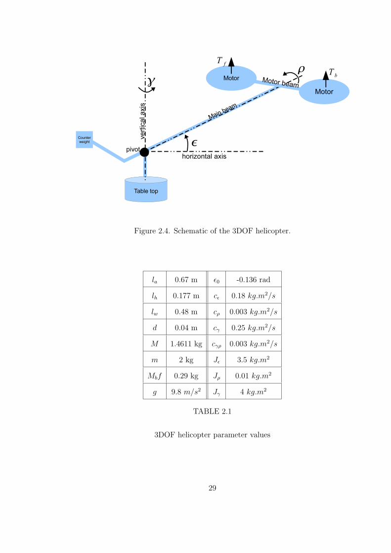
Figure 2.4. Schematic of the 3DOF helicopter.

la 0.67 m ϵ0 -0.136 rad

lh 0.177 m cϵ 0.18 kg.m2/s

lw 0.48 m cρ 0.003 kg.m2/s

d 0.04 m cγ 0.25 kg.m2/s

M 1.4611 kg cγρ 0.003 kg.m2/s

m 2 kg Jϵ 3.5 kg.m2

Mbf 0.29 kg Jρ 0.01 kg.m2

g 9.8 m/s2 Jγ 4 kg.m2

TABLE 2.1

3DOF helicopter parameter values

29

The system dynamic is described by the following equations [7].

Jϵϵm =−√((mlw −Mla)g)2 + ((m+M)gd)2 sin(ϵm)

+ Tcol cos(ρ)(la + d tan(ϵm + ϵ0))− cϵϵm,

Jρρ =Tcyclh −Mbfgd sin(ρ)− cρρ+ cγργ,

Jγ γ =− laTcol sin ρ cos ϵ− cγ γ,

and the elevation, pitch and travel rate can be directly measured with the measure-

ment noises to be white zero mean Gaussian, and the variances of the measurement

noises are 1.857× 10−6, 1.857× 10−6, and 1.857× 10−6, respectively.

In this model, ϵm = ϵ − ϵ0, m is the gross counter weight at the tail, M is the

gross weight at the head, Mbf = mb +mf is the sum mass of the two motors, lw is

the length from the pivot to the tail while la is the length from the pivot to the head,

d is some adjusted length with respect to the elevation, g is the gravity acceleration,

Tcol = Tf + Tb and Tcyc = Tb − Tf are the collective and cyclic thrusts, cϵϵ, cρρ, cγργ,

cγ γ are the drags generated by air due to the change of elevation, pitch and travel,

and Jϵ, Jρ and Jγ are the inertia moments for elevation, pitch and travel respectively.

The parameter values are given in Table 2.1.

Neglecting the non-dominant terms and under the assumption that sin(ρ) ≈ ρ

and sin(ϵm) ≈ ϵm, the model of 3DOF helicopter can be linearized as

Jϵϵm =−√

((mlw −Mla)g)2 + ((m+M)gd)2ϵm − cϵϵm + lauϵm (2.26)

Jρρ =−Mbfgdρ− cρρ− cγργ + lhuρ (2.27)

Jγ γ =− cγ γ − lauγ, (2.28)

where uϵm , uρ and uγ are the control inputs for elevation, pitch and travel subsystems

30

satisfying

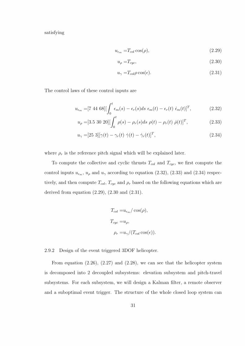
uϵm =Tcol cos(ρ), (2.29)

uρ =Tcyc, (2.30)

uγ =Tcolρ cos(ϵ). (2.31)

The control laws of these control inputs are

uϵm =[7 44 68][

∫ t

0

ϵm(s)− ϵr(s)ds ϵm(t)− ϵr(t) ϵm(t)]T , (2.32)

uρ =[3.5 30 20][

∫ t

0

ρ(s)− ρr(s)ds ρ(t)− ρr(t) ρ(t)]T , (2.33)

uγ =[25 3][γ(t)− γr(t) γ(t)− γr(t)]T , (2.34)

where ρr is the reference pitch signal which will be explained later.

To compute the collective and cyclic thrusts Tcol and Tcyc, we first compute the

control inputs uϵm , uρ and uγ according to equation (2.32), (2.33) and (2.34) respec-

tively, and then compute Tcol, Tcyc and ρr based on the following equations which are

derived from equation (2.29), (2.30 and (2.31).

Tcol =uϵm/ cos(ρ),

Tcyc =uρ,

ρr =uγ/(Tcol cos(ϵ)).

2.9.2 Design of the event triggered 3DOF helicopter.

From equation (2.26), (2.27) and (2.28), we can see that the helicopter system

is decomposed into 2 decoupled subsystems: elevation subsystem and pitch-travel

subsystems. For each subsystem, we will design a Kalman filter, a remote observer

and a suboptimal event trigger. The structure of the whole closed loop system can

31

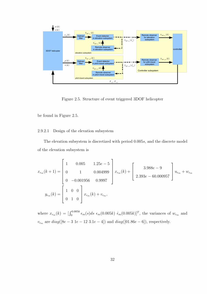
Figure 2.5. Structure of event triggered 3DOF helicopter

be found in Figure 2.5.

2.9.2.1 Design of the elevation subsystem

The elevation subsystem is discretized with period 0.005s, and the discrete model

of the elevation subsystem is

xϵm(k + 1) =

1 0.005 1.25e− 5

0 1 0.004999

0 −0.001956 0.9997

xϵm(k) +

3.988e− 9

2.393e− 60.000957

uϵm + wϵm

yϵm(k) =

1 0 0

0 1 0

xϵm(k) + vϵm ,

where xϵm(k) = [∫ 0.005k

0ϵm(s)ds ϵm(0.005k) ϵm(0.005k)]

T , the variances of wϵm and

vϵm are diag([8e− 3 1e− 12 3.1e− 4]) and diag([01.86e− 6]), respectively.

32

subsystem elapsed time foroperating 2.25

upper bound J lower boundon minimum

cost J∗

JJ∗

elevation ≈ 40s 0.20 0.076 2.65

pitch-travel ≈ 630 0.67 0.16 4.18

TABLE 2.2

Upper bound on the suboptimal cost and lower bound on the minimum cost

By solving the discrete linear Riccati equation, we have the Kalman filter gain as

Lϵm =

1 0.0016

0 0.3563

0 10.77

.

Algorithm 2.7.6 was, then, used to compute a suboptimal event trigger. Let

the weight matrix Z = diag([1 6 1]), λ = 1, ϕ = 2, δ = 1. h2 was chosen to be

a polynomial which contains all possible monomials whose degree is even and no

greater than 10.

A lower bound on the minimum cost was computed based on the SOS program-

ming 2.21. In this Algorithm, h1 was chosen to be a polynomial which contains all

possible monomials whose degree is no greater than 10.The related results about the upper bound on the suboptimal cost and lower

bound on the minimum cost are given in Table 2.2. From the last column of thistable, we find that the upper bound on the suboptimal cost is 2.65 times of the lowerbound on the optimal cost, which is considered to be acceptable.

33

2.9.2.2 Design of the pitch-travel subsystem

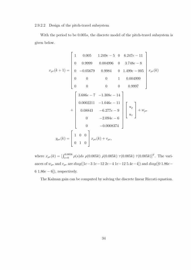
With the period to be 0.005s, the discrete model of the pitch-travel subsystem is

given below.

xρτ (k + 1) =

1 0.005 1.249e− 5 0 6.247e− 11

0 0.9999 0.004996 0 3.748e− 8

0 −0.05679 0.9984 0 1.499e− 005

0 0 0 1 0.004999

0 0 0 0 0.9997

xρτ (k)

+

3.686e− 7 −1.308e− 14

0.0002211 −1.046e− 11

0.08843 −6.277e− 9

0 −2.094e− 6

0 −0.0008374

uρ

uτ

+ wρτ

yρτ (k) =

1 0 0

0 1 0

xρτ (k) + vρτ ,

where xρτ (k) = [∫ 0.005k

s=0ρ(s)ds ρ(0.005k) ρ(0.005k) τ(0.005k) τ(0.005k)]T . The vari-

ances of wρτ and vρτ are diag([1e−3 1e−12 2e−4 1e−12 5.4e−4]) and diag([0 1.86e−

6 1.86e− 6]), respectively.

The Kalman gain can be computed by solving the discrete linear Riccati equation.

34

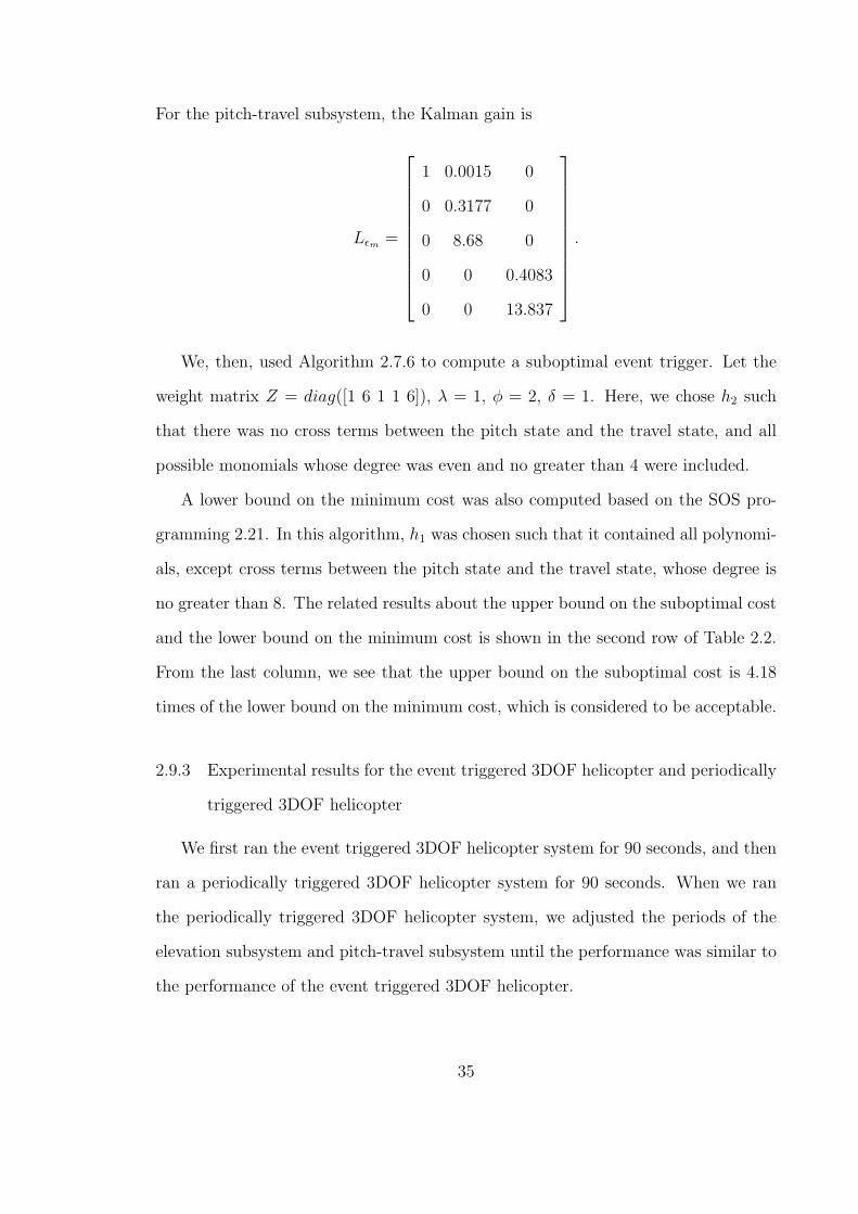
For the pitch-travel subsystem, the Kalman gain is

Lϵm =

1 0.0015 0

0 0.3177 0

0 8.68 0

0 0 0.4083

0 0 13.837

.

We, then, used Algorithm 2.7.6 to compute a suboptimal event trigger. Let the

weight matrix Z = diag([1 6 1 1 6]), λ = 1, ϕ = 2, δ = 1. Here, we chose h2 such

that there was no cross terms between the pitch state and the travel state, and all

possible monomials whose degree was even and no greater than 4 were included.

A lower bound on the minimum cost was also computed based on the SOS pro-

gramming 2.21. In this algorithm, h1 was chosen such that it contained all polynomi-

als, except cross terms between the pitch state and the travel state, whose degree is

no greater than 8. The related results about the upper bound on the suboptimal cost

and the lower bound on the minimum cost is shown in the second row of Table 2.2.

From the last column, we see that the upper bound on the suboptimal cost is 4.18

times of the lower bound on the minimum cost, which is considered to be acceptable.

2.9.3 Experimental results for the event triggered 3DOF helicopter and periodically

triggered 3DOF helicopter

We first ran the event triggered 3DOF helicopter system for 90 seconds, and then

ran a periodically triggered 3DOF helicopter system for 90 seconds. When we ran

the periodically triggered 3DOF helicopter system, we adjusted the periods of the

elevation subsystem and pitch-travel subsystem until the performance was similar to

the performance of the event triggered 3DOF helicopter.

35

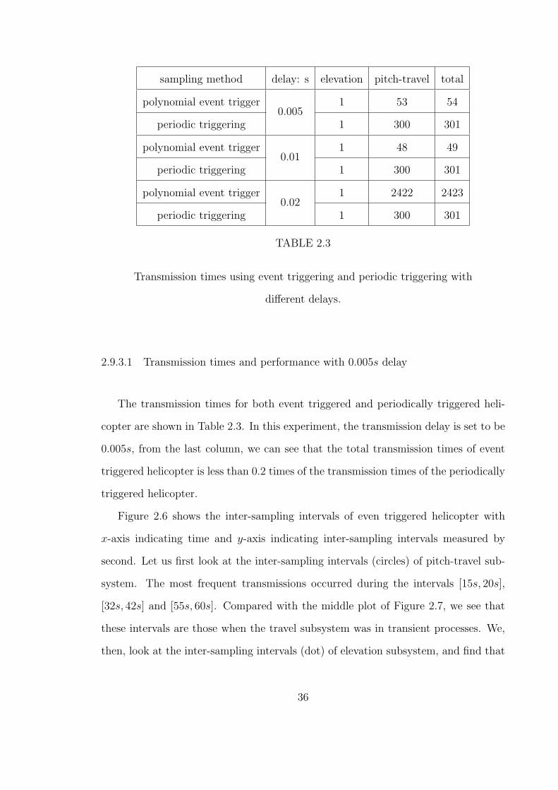
sampling method delay: s elevation pitch-travel total

polynomial event trigger0.005

1 53 54

periodic triggering 1 300 301


1 48 49



1 2422 2423


TABLE 2.3

Transmission times using event triggering and periodic triggering with

different delays.

2.9.3.1 Transmission times and performance with 0.005s delay

The transmission times for both event triggered and periodically triggered heli-

copter are shown in Table 2.3. In this experiment, the transmission delay is set to be

0.005s, from the last column, we can see that the total transmission times of event

triggered helicopter is less than 0.2 times of the transmission times of the periodically

triggered helicopter.

Figure 2.6 shows the inter-sampling intervals of even triggered helicopter with

x-axis indicating time and y-axis indicating inter-sampling intervals measured by

second. Let us first look at the inter-sampling intervals (circles) of pitch-travel sub-

system. The most frequent transmissions occurred during the intervals [15s, 20s],

[32s, 42s] and [55s, 60s]. Compared with the middle plot of Figure 2.7, we see that

these intervals are those when the travel subsystem was in transient processes. We,

then, look at the inter-sampling intervals (dot) of elevation subsystem, and find that

36

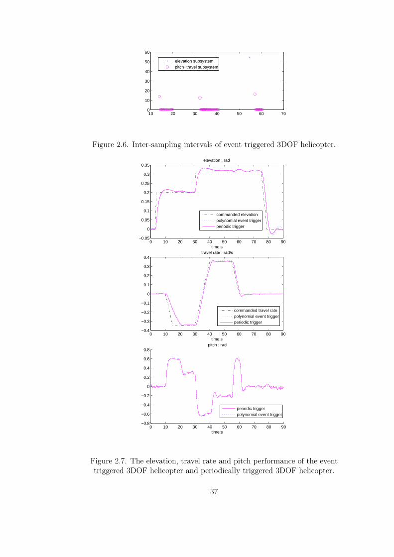
10 20 30 40 50 60 700

10

20

30

40

50

60

elevation subsystempitch−travel subsystem

Figure 2.6. Inter-sampling intervals of event triggered 3DOF helicopter.

0 10 20 30 40 50 60 70 80 90−0.05

0

0.05

0.1

0.15

0.2

0.25

0.3

0.35elevation : rad

time:s

commanded elevationpolynomial event triggerperiodic trigger

0 10 20 30 40 50 60 70 80 90−0.4

−0.3

−0.2

−0.1

0

0.1

0.2

0.3

0.4travel rate : rad/s

time:s

commanded travel ratepolynomial event triggerperiodic trigger

0 10 20 30 40 50 60 70 80 90−0.8

−0.6

−0.4

−0.2

0

0.2

0.4

0.6

0.8pitch : rad

time:s

periodic triggerpolynomial event trigger

Figure 2.7. The elevation, travel rate and pitch performance of the eventtriggered 3DOF helicopter and periodically triggered 3DOF helicopter.

37

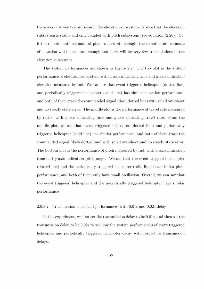
there was only one transmission in the elevation subsystem. Notice that the elevation

subsystem is stable and only coupled with pitch subsystem (see equation (2.26)). So,

if the remote state estimate of pitch is accurate enough, the remote state estimate

of elevation will be accurate enough and there will be very few transmissions in the

elevation subsystem.

The system performances are shown in Figure 2.7. The top plot is the system

performance of elevation subsystem, with x-axis indicating time and y-axis indication

elevation measured by rad. We can see that event triggered helicopter (dotted line)

and periodically triggered helicopter (solid line) has similar elevation performance,

and both of them track the commanded signal (dash dotted line) with small overshoot

and no steady state error. The middle plot is the performance of travel rate measured

by rad/s, with x-axis indicating time and y-axis indicating travel rate. From the

middle plot, we see that event triggered helicopter (dotted line) and periodically

triggered helicopter (solid line) has similar performance, and both of them track the

commanded signal (dash dotted line) with small overshoot and no steady state error.

The bottom plot is the performance of pitch measured by rad, with x-axis indication

time and y-axis indication pitch angle. We see that the event triggered helicopter

(dotted line) and the periodically triggered helicopter (solid line) have similar pitch

performance, and both of them only have small oscillation. Overall, we can say that

the event triggered helicopter and the periodically triggered helicopter have similar

performance.

2.9.3.2 Transmission times and performances with 0.01s and 0.02s delay

In this experiment, we first set the transmission delay to be 0.01s, and then set the

transmission delay to be 0.02s to see how the system performances of event triggered

helicopter and periodically triggered helicopter decay with respect to transmission

delays.

38

0 10 20 30 40 50 60 70 80 90−0.1

0

0.1

0.2

0.3

0.4elevation : rad

time:s


0 10 20 30 40 50 60 70 80 90−0.4

−0.3

−0.2

−0.1

0

0.1

0.2

0.3


time:s


0 10 20 30 40 50 60 70 80 90−1

−0.5

0

0.5

1pitch : rad

time:s


Figure 2.8. System performance with 0.01s delay

39

0 10 20 30 40 50 60 70 80 90−0.1

0

0.1

0.2

0.3

0.4elevation : rad

time:s


0 10 20 30 40 50 60 70 80 90−0.4

−0.3

−0.2

−0.1

0

0.1

0.2

0.3


time:s


0 10 20 30 40 50 60 70 80 90−0.8

−0.6

−0.4

−0.2

0

0.2

0.4

0.6pitch : rad

time:s


Figure 2.9. System performance with 0.02s delay

40

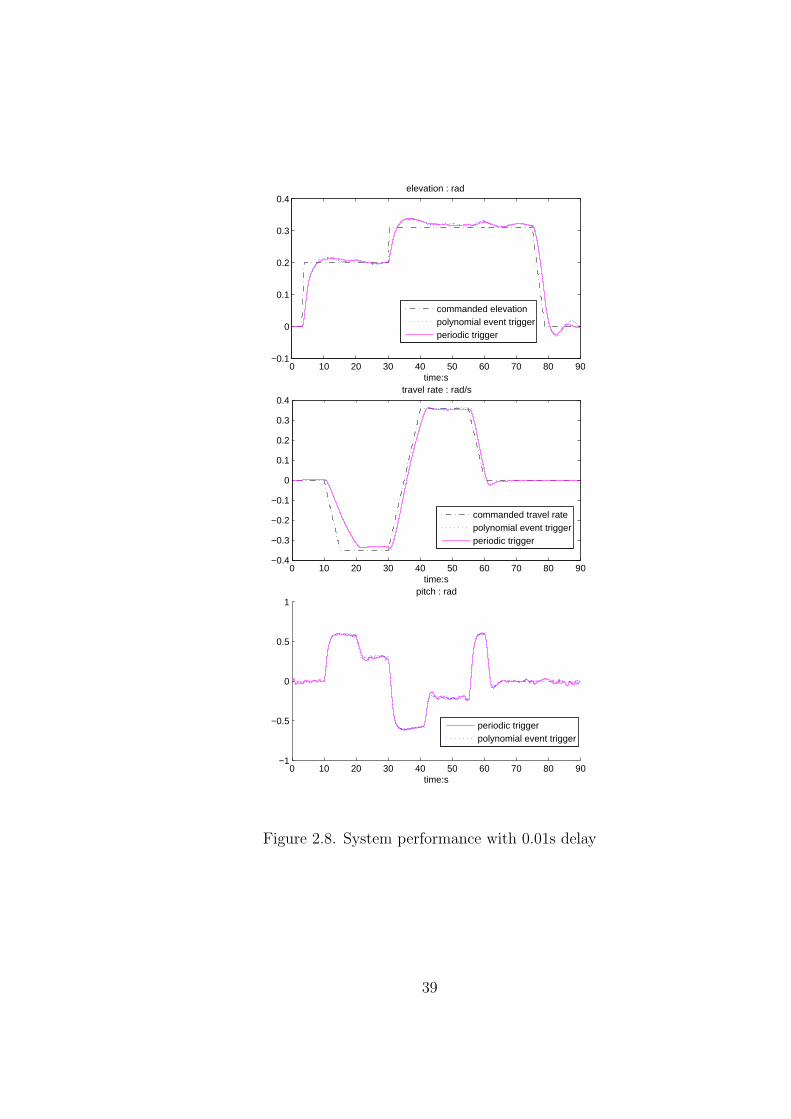
In the presence of 0.01s delay, the system performances of both event triggered

3DOF helicopter and periodically triggered 3DOF helicopter are shown in Figure 2.8.

The top plot is the performance of the elevation subsystem, the middle plot is the

performance of travel rate, and the bottom plot is the performance of pitch. In these

three plots, solid lines are performances of periodically triggered helicopter, dotted

lines are performances of event triggered helicopter, and dash dotted lines are com-

manded signals. From the three plots of Figure 2.8, we can see that in the presence

of 0.01s delay, the performance of event triggered helicopter is similar to the perfor-

mance of periodically triggered helicopter, and both of them tracked the commanded

elevation and travel rate with small overshoot and no steady state error with small

oscillation in the pitch angle. Now, let us look at the transmission times of both

event triggered helicopter and periodically triggered helicopter. The transmission

times are shown in the 3rd and 4th row of Table 2.3. We see that compared with

the periodically triggered helicopter system, the total transmission times in the event

triggered helicopter system is about 0.2 of the total transmission times in the periodi-

cally triggered helicopter system. Therefore, we conclude that when the transmission

delay is 0.01s, the event triggered helicopter and the periodically triggered helicopter

achieved similar performances while the event triggered helicopter transmitted less

than the periodically triggered helicopter.

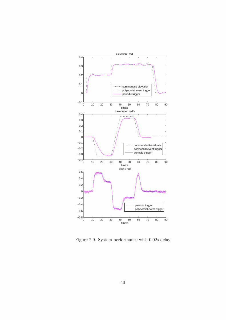
When the transmission delay is 0.02s, the system performances are shown in

Figure 2.9 with dotted lines indicating performances of the event triggered helicopter,

solid line indicating performances of the periodically triggered helicopter, and dash

dotted line indicating commanded signals. The top two plots are the performances

of elevation and travel rate, respectively. We see that event triggered helicopter and

periodically triggered helicopter had similar elevation and travel rate performance.

While both event triggered system and periodically triggered system tracked the

commanded elevation with small overshoot and no steady state error, there existed

41

steady state errors in travel rate for both event triggered system and periodically

triggered system. The bottom plot shows the performances of pitch. we can see that

the event triggered helicopter had smaller oscillation in pitch than the periodically

triggered helicopter. The transmission times of event triggered helicopter and the

periodically triggered helicopter are given in the 5th and 6th row of Table 2.3. We see

that in event triggered system, while the transmission times of elevation subsystem

remained at the same level, the transmission times of the pitch-travel subsystem

increase to 2422 from 54 (0.005s delay) and 49 (0.01s delay). This is because the

pitch angle kept oscillating, which means that the pitch subsystem was always in

a transient process. So, the pitch-travel subsystem kept transmitting information

during the whole running horizon. From Table 2.3, we see that event triggered

helicopter transmitted more than the periodically triggered helicopter, and the total

transmission times of event triggered helicopter is about 8 times of the transmission

times of the periodically triggered helicopter. From Figure 2.9 and Table 2.3, we

conclude that when the transmission delay is 0.02s, the event triggered helicopter

had better performance than the periodically triggered helicopter, but consumed

more communication resource than the periodically triggered helicopter.

2.10 Conclusion

This chapter provides computationally efficient, SOS programming based algo-

rithms to compute suboptimal event triggers, upper bounds on the suboptimal costs,

and lower bounds on the optimal costs. These SOS programming based algorithms

are effective for both stable and unstable systems. Our simulation results show that

SOS program (2.21) and (2.25) can compute tighter lower bound on the optimal cost

and tighter upper bound on the suboptimal cost than the prior work [14, 12, 35],

while guaranteeing almost the same actual cost as the prior work [14, 12, 35]. The

algorithms are, then, applied to an 8 dimensional nonlinear 3DOF helicopter. The

42

simulation results show that the event triggered helicopter uses less communication

resource than periodically triggered helicopter to achieve similar performance, and

tolerates the same amount of delay. To our best knowledge, this is the first time

the approximation of the optimal event trigger has been applied to a system whose

dimension is greater than 2.

43

CHAPTER 3

MINIMUM MEAN SQUARE STATE WITH LIMITED TRANSMISSION

FREQUENCY

In last chapter, computationally efficient suboptimal event trigger is designed to

minimize the estimation error of the remote state estimate. In this chapter, we use

this remote state estimate to compute a control input, and then design an event

trigger for the remote controller to decide when to transmit the control input back

to the plant such that the mean square state is minimized. The proposed triggering

events only rely on local information so that the transmissions from the sensor and

controller subsystems are not necessarily synchronized. This represents an advance

over recent work in event-triggered output feedback control where transmission from

the controller subsystem was tightly coupled to the receipt of event-triggered sensor

data. The paper presents an upper bound on the optimal cost attained by the closed-

loop system. Simulation results demonstrate that transmissions between sensors and

controller subsystems are not tightly synchronized. These results are also consistent

with derived upper bounds on overall system cost.

3.1 Introduction

Most prior work in the event triggering literature discusses state feedback control

and state estimation. This work has traditionally assumed a single feedback link in

the system. It has only been very recently that researchers have turned to study event-

triggered output feedback control where there are separate communication channels

from sensor to controller and controller to actuator. If we design triggering events

44

for both communication channels, an interesting question to ask is how these two

triggering events are coupled with each other.

Some of the work in event triggered output feedback systems hid this question by

assuming that only part of the control loop was closed over communication channel,

i.e. either sensor-to-controller link or controller-to-actuator link is connected directly

[34, 71, 48]. Another work in [16] assumed very strong coupling between the trigger-

ing rules of sensor-to-controller link and controller-to-actuator link. They required

that the transmission in one link triggered the transmission in the other link, so

transmissions in both communication channels are synchronized.

This synchronization is not necessary. This chapter examines a weakly coupled

event triggered system. We study optimal event triggers that minimize the mean

square cost of the system state discounted by the communication cost in both links.

By realizing that the remote state estimate is orthogonal to the remote state esti-

mation error, the optimal cost of the output feedback system is decomposed into

the optimal cost of a state estimation problem and the optimal cost of a state feed-

back problem. This paper first gives the optimal event-triggers for both the state

estimation problem and the state feedback problem. Because of the computational

complexity of the optimal event triggers, computationally efficient suboptimal event

triggers and the upper bounds on associated costs are, then, provided.

Compared with the synchronized design, there are two advantages of this weakly

coupled design, especially in large scale multi-sensor systems. The first advantage

is that this weakly coupled design has the potential to reduce the communication

cost a lot in large scale multi-sensor systems. With weakly coupled design, sensors

only transmit information when the remote estimation error is large enough, and

the controller only transmit information when the remote state estimate and the

actual control input are large enough. With synchronized design, when the controller

transmits its control signal, all sensors have to transmit sensor information, even

45

though some of the sensors may have just finished their transmissions. At the same

time, in a large scale multi-sensor system, the controller receives information from

all the sensors. It is very possible that several sensor signals arrive in a short time.

With synchronized design, the controller has to transmit very similar control signals

several times in a short time. All these cases in synchronized design is a waste of

communication resources, which can be easily avoided by the weakly coupled design.

The second advantage of the weakly coupled design is to reduce the scheduling burden

of the controller with synchronized design in large scale multi-sensor systems. With

synchronized design, as the number of sensors increases, the transmission frequency of

the controller also increases, and the controller has to schedule the transmission tasks

more and more often, which increases the scheduling burden of the controller. While

with the weakly coupled design, since the controller only transmits when the remote

state estimate and the control signal are large enough, the controller will not schedule

the transmission tasks more frequently, as long as the dynamic of the system, the

system noises and the measurement noises remain at the same level. So, compared

with synchronized design, the weakly coupled design reduces the scheduling burden

of the controller in large scale multi-sensor systems.

3.2 Problem Statement

Consider a system shown in Figure 3.1. The plant is a discrete time linear time

invariant system described by the following difference equation.

x(k) = Ax(k − 1) +Bua(k − 1) + w(k − 1),

y(k) = Cx(k) + v(k),∀k = 1, 2, · · · ,

where x ∈ Rn is the state with its initial condition Gaussian distributed with mean

µ0 and variance π0, y ∈ Rp is the measurement, ua ∈ Rm is the control input applied

46

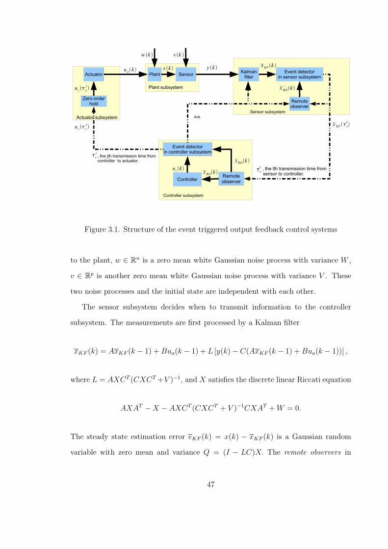
Figure 3.1. Structure of the event triggered output feedback control systems

to the plant, w ∈ Rn is a zero mean white Gaussian noise process with variance W ,

v ∈ Rp is another zero mean white Gaussian noise process with variance V . These

two noise processes and the initial state are independent with each other.

The sensor subsystem decides when to transmit information to the controller

subsystem. The measurements are first processed by a Kalman filter

xKF (k) = AxKF (k − 1) +Bua(k − 1) + L [y(k)− C(AxKF (k − 1) +Bua(k − 1))] ,

where L = AXCT (CXCT +V )−1, and X satisfies the discrete linear Riccati equation

AXAT −X − AXCT (CXCT + V )−1CXAT +W = 0.

The steady state estimation error eKF (k) = x(k) − xKF (k) is a Gaussian random

variable with zero mean and variance Q = (I − LC)X. The remote observers in

47

both sensor and controller subsystems generate an a priori remote state estimate

x−RO(k) and an a posteriori remote state estimate xRO(k). The gap e−KF,RO(k) =

xKF (k)− x−RO(k) is, then, used by the event detector to decide whether to transmit

the current xKF (k) to the remote observer. Let as(k) = 1 indicate the decision of

transmitting xKF (k), and 0 otherwise. We force as(k) = 1 if ∥e−KF,RO(k)∥ > θs for

a large positive constant θs. The lth transmission time of the sensor subsystem is

denoted as τ ls.

The controller subsystem produces the control input, and decides when to trans-

mit the current control input. The remote observer takes the form of

x−RO(k) =AxRO(k − 1) +Bua(k − 1), with x−(0) = µ0 (3.1)

xRO(k) =

x−RO(k), if as(k) = 0;

xKF (k), if as(k) = 1 ,(3.2)

It is easy to show through mathematical induction that this is the minimum mean

square estimate of x based on all history information of the controller (please check

Lemma A.0.2 in Appendix for the proof). The controller generates a control input

uc(k) = KxRO(k),

where K is the controller gain. The event detector in the controller subsystem, then,

uses the augmented vector [xRO(k) ua(k − 1)]T to decide whether to transmit the

current control input uc(k) to the plant. Let ac(k) = 1 indicate the decision of

transmitting uc(k), and 0 otherwise. We force ac(k) = 1 if ∥[xRO(k) ua(k−1)]T )∥ > θc

for a large positive constant θc. Once the controller subsystem decides to transmit

uc(k), an acknowledgement is also transmitted to the sensor subsystem. The jth

transmission time from controller to actuator is denoted by τ jc .

When uc(τjc ) is transmitted, the actuator subsystem updates ua(k) to be uc(τ

jc ),

48

and holds this value until the next transmission occurs. ua(k), then, satisfies

ua(k) = uc(τjc ), ∀k = τ jc , . . . , τ

j+1c − 1. (3.3)

The average cost is defined as

J(as(k)∞k=0, ac(k)∞k=0) = limN→∞

1

N

N−1∑k=0

E (c(x(k), as(k), ac(k))) ,

where the cost function

c(x(k), as(k), ac(k)) = ∥x(k)∥2Z + λsas(k) + λcac(k),

where Z ∈ Rn×n is a positive definite matrix, ∥x(k)∥2Z = xTZx, λs and λc are

the communication prices for transmissions over the sensor-to-controller link and

controller-to-actuator link, respectively.

Our objective is to find transmission rules for both the sensor subsystem and the

controller subsystem to minimize the average cost J(as(k)∞k=0, ac(k)∞k=0), i.e.

J∗ = minas(k)∞k=0,ac(k)

∞k=0

J(as(k)∞k=0, ac(k)∞k=0).

3.3 Decomposition of the average cost

This section shows that the average cost J can be decomposed into a state esti-

mation cost and a control cost.

Let eRO(k) = x(k) − xRO(k) be the remote state estimation error, and we have

the following lemma.

Lemma 3.3.1. eRO(k) is orthogonal to xRO(k) for all k ∈ Z+.

Proof. From Lemma A.0.2, we know that xRO(k) is a minimum mean square estimate

49

of the system state x(k), and hence the remote state estimation error eRO(k) is

orthogonal to xRO(k).

Based on the Lemma 3.3.1, the average cost is decomposed into a state estimation

cost and a control cost.

Theorem 3.3.2. The average cost

J(as(k)∞k=0, ac(k)∞k=0) = Js(as(k)∞k=0) + Jc(ac(k)∞k=0),

where

Js(as(k)∞k=0) = limN→∞

1

N

N−1∑k=0

E[∥eRO(k)∥2Z + λsas(k)

],

Jc(ac(k)∞k=0) = limN→∞

1

N

N−1∑k=0

E[∥xRO(k)∥2Z + λcac(k).

]Proof. According to Lemma 3.3.1, the average cost J(as(k)∞k=0, ac(k)∞k=0) is rewrit-

ten as

J(as(k)∞k=0, ac(k)∞k=0) = limN→∞

1

N

N−1∑k=0

E(∥eRO(k)∥2Z + λsas(k)

+∥xRO(k)∥2Z + λcac(k))

=Js(as(k)∞k=0) + Jc(ac(k)∞k=0).

Js(as(k)∞k=0) relies on the remote state estimation error and the communica-

tion price between sensor and controller, and is called the state estimation cost.

Jc(ac(k)∞k=0) relies on the remote state estimate and the communication price be-

tween controller and actuator, and is called the control cost.

50

Remark 3.3.3. Both the state estimation cost and the control cost depend on the

communication decision as(k) in the sensor subsystem. It is easy to see that the state

estimation cost Js relies on as(k). The control cost Jc also relies on as(k), because Jc

must be computed with respect to the remote state estimate, xRO(k), which is related

to as(k) according to equation (2.12). To emphasize the dependence of the control

cost on the communication decision as(k) in the sensor subsystem, we rewrite the the

control cost as Jc(as(k)∞k=0) = Jc(as(k)∞k=0, ac(k)∞k=0).

Let a†s be the optimal transmission rule that minimizes Js with the corresponding

optimal cost J†s , and a†c be the controller’s optimal communication strategy that

minimizes the controller cost Jc based on a†s with the corresponding control cost

J†c (a

†s). Since Js and Jc are coupled, we see that the minimum cost J∗ is bounded

above by

J∗ ≤ J(a†s, a†c) = J†

s + J†c (a

†s). (3.4)

3.4 The Optimal Event Triggers

This section provides the optimal communication rule a†s for the sensor subsystem

and the optimal communication rule a†c for the controller subsystem based on a†s.

3.4.1 The Optimal Event Trigger in The Sensor Subsystem

Let eKF,RO(k) = xKF (k) − xRO(k) be the a posteriori gap between the filtered

state and the remote state estimate. Noticing that eKF,RO(k) is orthogonal to the

filtered state error eKF (k) (please check Lemma A.0.1 in Appendix for the proof),

together with the dynamic behavior of xKF and x−RO, the estimation cost is rewritten

51

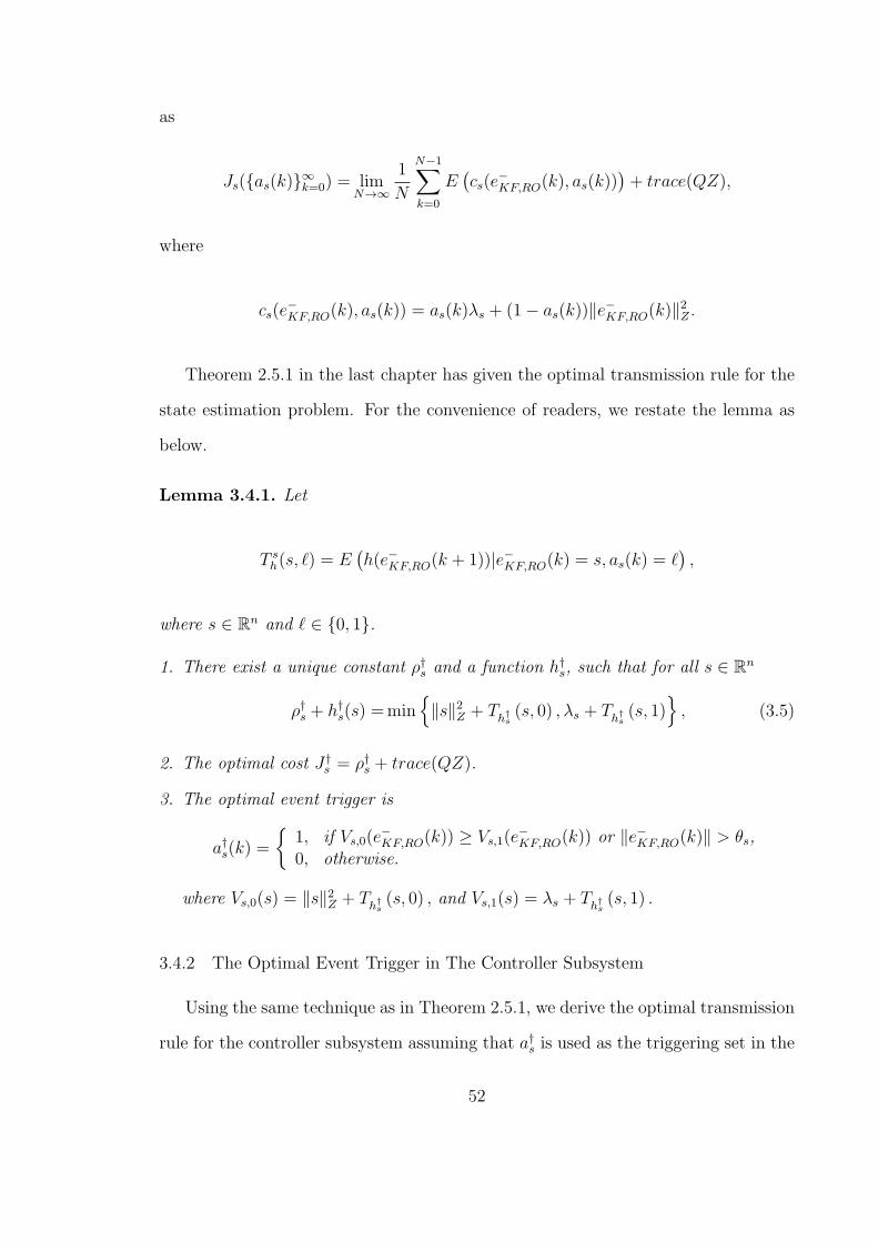
as

Js(as(k)∞k=0) = limN→∞

1

N

N−1∑k=0

E(cs(e

−KF,RO(k), as(k))

)+ trace(QZ),

where

cs(e−KF,RO(k), as(k)) = as(k)λs + (1− as(k))∥e−KF,RO(k)∥

2Z .

Theorem 2.5.1 in the last chapter has given the optimal transmission rule for the

state estimation problem. For the convenience of readers, we restate the lemma as

below.

Lemma 3.4.1. Let

T sh(s, ℓ) = E

(h(e−KF,RO(k + 1))|e−KF,RO(k) = s, as(k) = ℓ

),

where s ∈ Rn and ℓ ∈ 0, 1.

1. There exist a unique constant ρ†s and a function h†s, such that for all s ∈ Rn

ρ†s + h†s(s) =min

∥s∥2Z + Th†

s(s, 0) , λs + Th†

s(s, 1)

, (3.5)

2. The optimal cost J†s = ρ†s + trace(QZ).


a†s(k) =

1, if Vs,0(e

−KF,RO(k)) ≥ Vs,1(e

−KF,RO(k)) or ∥e−KF,RO(k)∥ > θs,

0, otherwise.

where Vs,0(s) = ∥s∥2Z + Th†s(s, 0) , and Vs,1(s) = λs + Th†

s(s, 1) .

3.4.2 The Optimal Event Trigger in The Controller Subsystem

Using the same technique as in Theorem 2.5.1, we derive the optimal transmission

rule for the controller subsystem assuming that a†s is used as the triggering set in the

52

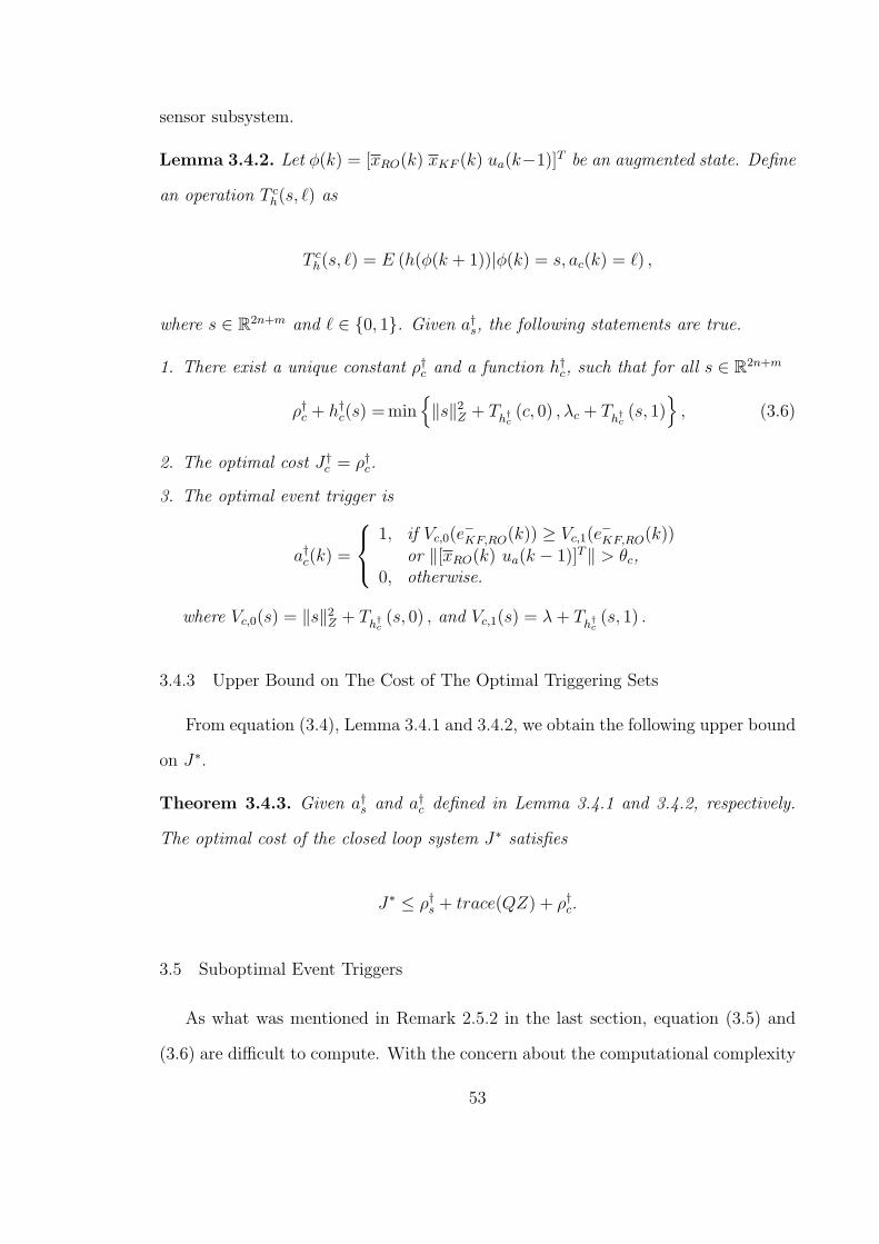
sensor subsystem.

Lemma 3.4.2. Let ϕ(k) = [xRO(k) xKF (k) ua(k−1)]T be an augmented state. Define

an operation T ch(s, ℓ) as

T ch(s, ℓ) = E (h(ϕ(k + 1))|ϕ(k) = s, ac(k) = ℓ) ,

where s ∈ R2n+m and ℓ ∈ 0, 1. Given a†s, the following statements are true.

1. There exist a unique constant ρ†c and a function h†c, such that for all s ∈ R2n+m

ρ†c + h†c(s) =min

∥s∥2Z + Th†

c(c, 0) , λc + Th†

c(s, 1)

, (3.6)

2. The optimal cost J†c = ρ†c.


a†c(k) =

1, if Vc,0(e

−KF,RO(k)) ≥ Vc,1(e

−KF,RO(k))

or ∥[xRO(k) ua(k − 1)]T∥ > θc,0, otherwise.

where Vc,0(s) = ∥s∥2Z + Th†c(s, 0) , and Vc,1(s) = λ+ Th†

c(s, 1) .

3.4.3 Upper Bound on The Cost of The Optimal Triggering Sets

From equation (3.4), Lemma 3.4.1 and 3.4.2, we obtain the following upper bound

on J∗.

Theorem 3.4.3. Given a†s and a†c defined in Lemma 3.4.1 and 3.4.2, respectively.

The optimal cost of the closed loop system J∗ satisfies

J∗ ≤ ρ†s + trace(QZ) + ρ†c.

3.5 Suboptimal Event Triggers

As what was mentioned in Remark 2.5.2 in the last section, equation (3.5) and

(3.6) are difficult to compute. With the concern about the computational complexity

53

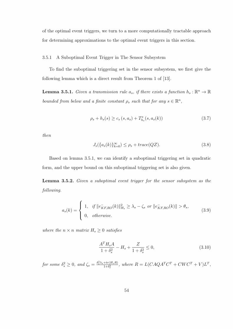
of the optimal event triggers, we turn to a more computationally tractable approach

for determining approximations to the optimal event triggers in this section.

3.5.1 A Suboptimal Event Trigger in The Sensor Subsystem

To find the suboptimal triggering set in the sensor subsystem, we first give the

following lemma which is a direct result from Theorem 1 of [13].

Lemma 3.5.1. Given a transmission rule as, if there exists a function hs : Rn → R

bounded from below and a finite constant ρs such that for any s ∈ Rn,

ρs + hs(s) ≥ cs (s, as) + T shs(s, as(k)) (3.7)

then

Js(as(k)∞k=0) ≤ ρs + trace(QZ). (3.8)

Based on lemma 3.5.1, we can identify a suboptimal triggering set in quadratic

form, and the upper bound on this suboptimal triggering set is also given.

Lemma 3.5.2. Given a suboptimal event trigger for the sensor subsystem as the

following.

as(k) =

1, if ∥e−KF,RO(k)∥2Hs≥ λs − ζs or ∥e−KF,RO(k)∥ > θs,

0, otherwise.(3.9)

where the n× n matrix Hs ≥ 0 satisfies

ATHsA

1 + δ2s−Hs +

Z

1 + δ2s≤ 0, (3.10)

for some δ2s ≥ 0, and ζs =δ2sλs+tr(HsR)

1+δ2s, where R = L(CAQATCT + CWCT + V )LT ,

54

then

Js(as(k)∞k=0) ≤ mintr(HsR) + ζs, λs+ tr(QZ) (3.11)

Proof. To find an upper bound on the cost of triggering set defined in equation (3.9),

we need to find a bounded function hs and a finite constant ρs such that equation

(3.7) is satisfied.

Now, let’s define hs as

hs(e−KF,RO(k)) = min∥e−KF,RO(k)∥

2Hs

+ ζs, λs,

and ρs as

ρs = E(hs(e−KF,RO(k + 1))|eKF,RO(k) = 0). (3.12)

In the case of ∥e−KF,RO(k)∥2Hs≤ λs − ζs, no transmission occurs at step k, so the

right hand side of equation (3.7) satisfies the following equations.

E(hs(e

−KF,RO(k + 1))|e−KF,RO(k), Ss

)+ cs

(e−KF,RO, Ss

)=E

(hs(e

−KF,RO(k + 1))|eKF,RO(k) = e−KF,RO(k)

)+ ∥e−KF,RO∥

2Z

≤∥e−KF,RO∥2ATHsA

+ tr(HsR) + ζs + ∥e−KF,RO∥2Z

≤∥e−KF,RO(k)∥2Hs

+ ∥e−KF,RO(k)∥2ATHsA−Hs+Z + ζs + tr(HsR)

≤∥e−KF,RO(k)∥2Hs

+ ζs + δ2s(λs − ζs) + tr(HsR)

=hs(e−KF,RO(k)) + ζs

≤hs(e−KF,RO(k)) + ρs.

The second step is taken by the fact that E(min(f, g)) ≤ min(E(f), E(g)), the fourth

step is derived from equation (3.10) and the fact that ∥e−KF,RO(k)∥2Hs≤ λs − ζs, and

55

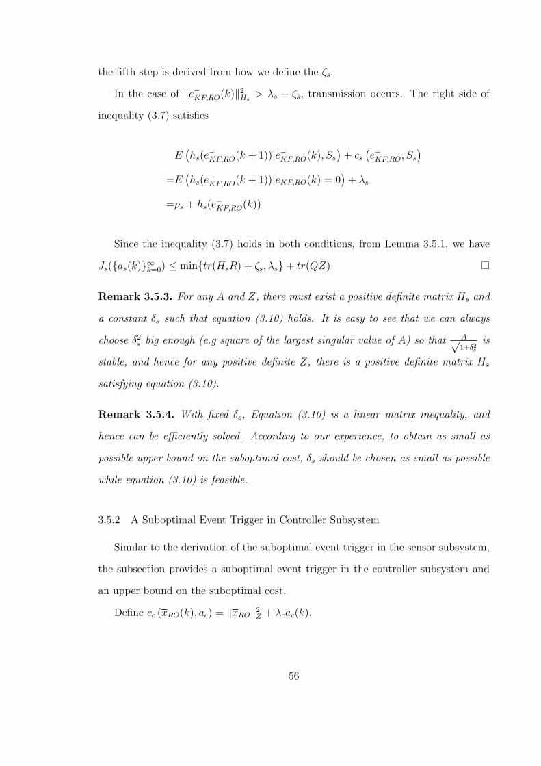
the fifth step is derived from how we define the ζs.

In the case of ∥e−KF,RO(k)∥2Hs> λs − ζs, transmission occurs. The right side of

inequality (3.7) satisfies

E(hs(e

−KF,RO(k + 1))|e−KF,RO(k), Ss

)+ cs

(e−KF,RO, Ss

)=E

(hs(e

−KF,RO(k + 1))|eKF,RO(k) = 0

)+ λs

=ρs + hs(e−KF,RO(k))

Since the inequality (3.7) holds in both conditions, from Lemma 3.5.1, we have

Js(as(k)∞k=0) ≤ mintr(HsR) + ζs, λs+ tr(QZ)

Remark 3.5.3. For any A and Z, there must exist a positive definite matrix Hs and

a constant δs such that equation (3.10) holds. It is easy to see that we can always

choose δ2s big enough (e.g square of the largest singular value of A) so that A√1+δ2s

is

stable, and hence for any positive definite Z, there is a positive definite matrix Hs

satisfying equation (3.10).

Remark 3.5.4. With fixed δs, Equation (3.10) is a linear matrix inequality, and

hence can be efficiently solved. According to our experience, to obtain as small as

possible upper bound on the suboptimal cost, δs should be chosen as small as possible

while equation (3.10) is feasible.

3.5.2 A Suboptimal Event Trigger in Controller Subsystem

Similar to the derivation of the suboptimal event trigger in the sensor subsystem,

the subsection provides a suboptimal event trigger in the controller subsystem and

an upper bound on the suboptimal cost.

Define cc (xRO(k), ac) = ∥xRO∥2Z + λcac(k).

56

Lemma 3.5.5. Given any communication rule ac, if there exists a function hc :

Rn × Rm → R bounded from below and a finite constant ρc such that

ρc + hc (ϕ(k)) ≥ cc (xRO(k), Sc) + T chc(ϕ(k), ac(k)), (3.13)

then Jc(ac(k)∞k=0) ≤ ρc.

Based on Lemma 3.5.5, the suboptimal event trigger in the controller subsystem

and its upper bound are provided in the following Lemma.

Lemma 3.5.6. Given the transmission rule as in the sensor subsystem defined in

Equation (3.9). Let Au =

A B

0 I

, Ac =

A+BK 0

K 0

, Za =

Z 0

0 0

, andHs = P T

HsPHs. Given the suboptimal event trigger for the controller subsystem as the

following.

ac(k) =

1, if

∥∥∥∥∥∥∥ xRO(k)

ua(k − 1)

∥∥∥∥∥∥∥2

Hc

+ ζc ≤ ∥xRO(k)∥2Z + λc

or ∥[xRO(k) ua(k − 1)]T∥ > θc,

0, otherwise.

(3.14)

where Hc ≥ Za and controller gain K satisfy

ATuHcAu + (1 + δ2c )(Za −Hc) ≤0, (3.15)

ATc HcAc + (1− ρ2c)(Za −Hc) ≤0, (3.16)

for some constant δ2c ≥ 0 and 0 ≤ α2c ≤ 1, and

ζc =δ2c + α2

c − 1

δ2c + α2c

λc. (3.17)

57

The controller cost satisfies

Jc(as(k)∞k=0, ac(k)∞k=0) ≤δ2c

δ2c + α2c

λc + σ((P THs)

−1Hc,luP−1Hs )(λs − ζs), (3.18)

where σ(·) indicates the greatest singular value, and Hc,lu is the left upper n × n

sub-matrix of Hc.

Proof. According to Lemma 3.5.5, as long as we can find a function hc bounded from

below and a finite constant ρc such that the inequality (3.13) is satisfied, Lemma

3.5.6 is true.

Let’s define

hc (xRO(k), ua(k − 1)) =

∥∥∥∥∥∥∥ xRO(k)

ua(k − 1)

∥∥∥∥∥∥∥2

Hc

+ ζc,

and

ρc =δ2c

δ2c + α2c

λc + σ((P THs)

−1Hc,luP−1Hs )(λs − ζs).

First, we consider the case when

∥∥∥∥∥∥∥ xRO(k)

ua(k − 1)

∥∥∥∥∥∥∥2

Hc

+ ζc ≤ ∥xRO(k)∥2Z + λc. In

this case, the controller subsystem doesn’t transmit. The right hand side of equation

58

(3.13) is

≤

xRO(k)

ua(k − 1)

T

ATuHcAu

xRO(k)

ua(k − 1)

+ σ((P THs)

−1Hc,luP−1Hs )(λs − ζs) + ζc

+

xRO(k)

ua(k − 1)

T

Za

xRO(k)

ua(k − 1)

≤ρc + fc

xRO(k)

ua(k − 1)

The first inequality is from equation (3.9), and the second inequality is from equation

(3.15) and (3.17).

The second case is when

∥∥∥∥∥∥∥ xRO(k)

ua(k − 1)

∥∥∥∥∥∥∥2

Hc

+ ζc > ∥xRO(k)∥2Z + λc. In this case,

the controller subsystem transmits information. So the right hand side of equation

(3.13) is

≤

xRO(k)

ua(k − 1)

T

ATc HcAc

xRO(k)

ua(k − 1)

+ σ((P THs)

−1Hc,luP−1Hs )(λs − ζs) + ζc

+

xRO(k)

ua(k − 1)

T

Za

xRO(k)

ua(k − 1)

+ λc

≤ρc + hc

xRO(k)

ua(k − 1)

.

The first inequality is from Equation (3.9), and the second inequality is from Equation

(3.16) and (3.17).

59

Since in both cases, equation (3.13) holds, we conclude that

Jc(as(k)∞k=0, ac(k)∞k=0) ≤ ρc.

3.5.3 An Upper Bound on The Total Suboptimal Cost

From the results in Lemma 3.3.2, 3.5.2 and 3.5.6, we have the following theorem.

Theorem 3.5.7. Given the event trigger as in the sensor subsystem defined in equa-

tion (3.9) and the event trigger ac in the controller subsystem defined in equation

(3.14), the average cost J(as(k)∞k=0, ac(k)∞k=0) given by the two weakly coupled

triggering sets satisfies

J(as(k)∞k=0, ac(k)∞k=0) ≤ ρs + trace(QZ) + ρc.

3.6 Simulation Results

This section uses an example to demonstrate Theorem 3.5.7. We first calculate

the triggering sets Ss and Sc according to equation (3.9) and (3.14), and search for

the controller gain K such that inequality (3.16) is satisfied. The system, then, is run

using three different transmission rules: weakly coupled event triggered transmission,

synchronized event triggered transmission and periodic transmission. The average

costs are compared. We also show that the number of transmission times in sensor

subsystem, the number of transmission times in controller subsystem, and the number

of times when both sensor and controller transmit (concurrent transmission times)

to illustrate that the transmission in the sensor subsystem doesn’t necessarily trigger

the transmission in the controller subsystem, or vice versa.

60

Let’s consider the following system

x(k) =

0.4 0

0 1.01

x(k − 1) +

1

1

ua(k − 1) + w(k − 1)

y(k) =

[0.1 1

]x(k) + v(k).

The variances of the system noises are W =

0.2 0.1

0.1 0.2

, and V = 0.3. The weight

matrix Z is chosen to be an identity matrix.

Given δ2s = 1.5, λs = 3, δ2c = 1.02 and ρc = 0.3, we can obtain the event trigger

as in sensor subsystem as

as(k) =

1, if e−T

KF,RO

2.5641 0

0 4.0543

e−KF,RO ≤ 0.8414 or ∥e−KF,RO(k)∥ > θs,

0, otherwise.

(3.19)

and the triggering set in controller subsystem Sc as

ac(k) =

1, if

xRO(k)

ua(k − 1)

T

1.3315 −0.2836 −0.3512

−0.2836 3.6377 2.6808

−0.3512 2.6808 13.7606

xRO(k)

ua(k − 1)

≤ 0.9008λc or ∥[xRO(k) ua(k − 1)]T∥ > θc,

0, otherwise.

(3.20)

and the controller gain K = [−0.1967 − 0.3133].

The closed loop system was run for 3000 steps using different transmission rules

with the communication price from controller to actuator varying from 0 to 200.

61

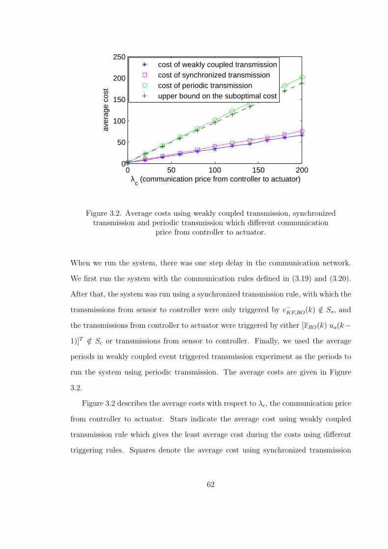
0 50 100 150 2000

50

100

150

200

250

λc (communication price from controller to actuator)

aver

age

cost

cost of weakly coupled transmissioncost of synchronized transmissioncost of periodic transmissionupper bound on the suboptimal cost

Figure 3.2. Average costs using weakly coupled transmission, synchronizedtransmission and periodic transmission which different communication

price from controller to actuator.

When we run the system, there was one step delay in the communication network.

We first run the system with the communication rules defined in (3.19) and (3.20).

After that, the system was run using a synchronized transmission rule, with which the

transmissions from sensor to controller were only triggered by e−KF,RO(k) /∈ Ss, and

the transmissions from controller to actuator were triggered by either [xRO(k) ua(k−

1)]T /∈ Sc or transmissions from sensor to controller. Finally, we used the average

periods in weakly coupled event triggered transmission experiment as the periods to

run the system using periodic transmission. The average costs are given in Figure

3.2.

Figure 3.2 describes the average costs with respect to λc, the communication price

from controller to actuator. Stars indicate the average cost using weakly coupled

transmission rule which gives the least average cost during the costs using different

triggering rules. Squares denote the average cost using synchronized transmission

62

rule which gives the second least average cost, and its difference from the average

cost of weakly coupled transmission increases as λc increases. That’s because when

λc is small, with synchronized transmission, most transmissions from controller to

actuator were triggered by the event [xRO(k) ua(k − 1)]T /∈ Sc, and hence synchro-

nized transmission had similar cost as the weakly coupled transmission. Figure 3.2

also shows that the average cost using periodic transmission (circles) is always greater

than the average cost using event triggered transmission no matter whether the trans-

mission is weakly coupled (stars) or synchronized (squares). Crosses are the upper

bounds on the average cost of weakly coupled transmission calculated according to

Theorem 3.5.7. These crosses are always above the average cost of weakly coupled

transmission (stars), which demonstrates Theorem 3.5.7. We also notice that both

the upper bound (crosses) and the actual cost (stars) increases linearly with respect

to λc, and the ratio of the upper bound (crosses) to the actual cost (stars) is about

3.

Figure 3.3 shows that the transmission in the sensor subsystem doesn’t always

trigger the transmission in controller subsystem, or vice versa. The x-axis of this plot

is the communication price from controller to actuator λc, and the y-axis indicates

the transmission times. We can see that the number of concurrent transmission

times (circles) is always less or equal to both the numbers of transmission times in

sensor subsystem (stars) and controller subsystem (crosses), which indicates that the

transmission in sensor subsystem doesn’t always trigger the transmission in controller

subsystem, or vice versa.

3.7 Conclusion

This paper presents weakly coupled triggering events in event triggered output

feedback system with the whole control loop closed over wireless network. By ’weakly

coupled’, we mean that the triggering events in both sensor and controller only use

63

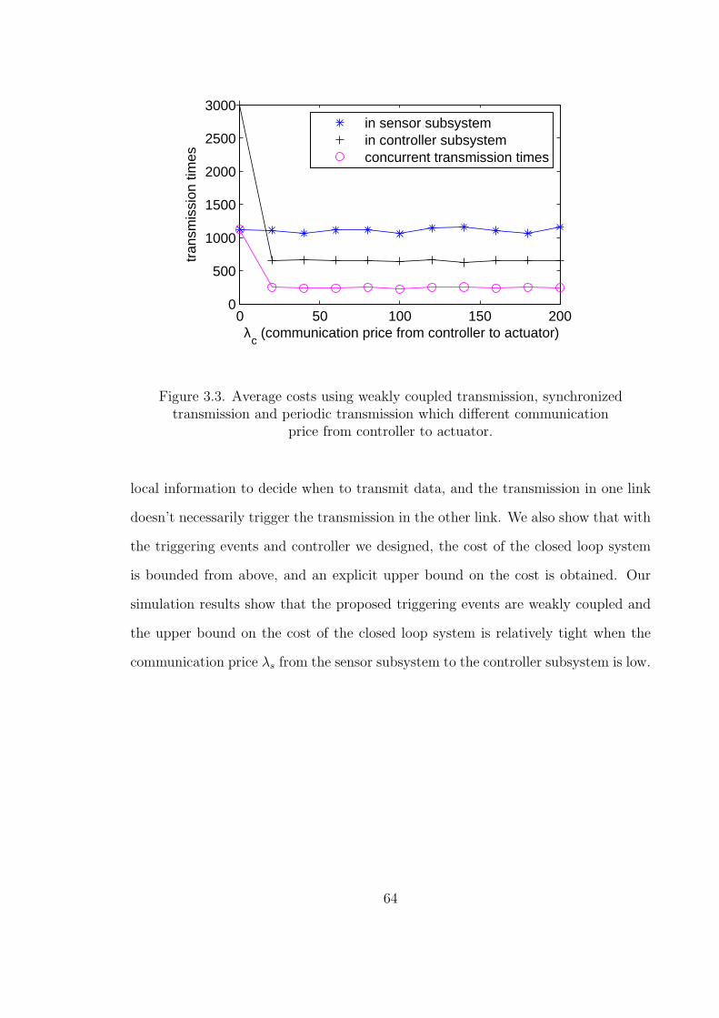
0 50 100 150 2000

500

1000

1500

2000

2500

3000

λc (communication price from controller to actuator)

tran

smis

sion

tim

es

in sensor subsystemin controller subsystemconcurrent transmission times

Figure 3.3. Average costs using weakly coupled transmission, synchronizedtransmission and periodic transmission which different communication

price from controller to actuator.

local information to decide when to transmit data, and the transmission in one link

doesn’t necessarily trigger the transmission in the other link. We also show that with

the triggering events and controller we designed, the cost of the closed loop system

is bounded from above, and an explicit upper bound on the cost is obtained. Our

simulation results show that the proposed triggering events are weakly coupled and

the upper bound on the cost of the closed loop system is relatively tight when the

communication price λs from the sensor subsystem to the controller subsystem is low.

64

CHAPTER 4

EFFICIENTLY ATTENTIVE AND ISS EVENT TRIGGERED CONTROL

SYSTEMS WITH LIMITED TRANSMISSION FREQUENCY AND

INSTANTANEOUS BIT-RATE

Chapter 2 and 3 study the minimum system performance cost with limited trans-

mission frequency. The network delay and quantization error, however, are neglected

in Chapter 2 and 3. This chapter explicitly considers the influence of network latency

and quantization error, and derives a bound on an event-triggered system’s stabiliz-

ing ‘instantaneous’ bit-rate when the sampled signal is dynamically quantized. This

instantaneous bit-rate is a time-varying function whose average value can be made

small by requiring the instantaneous bit-rate get smaller as the system state ap-

proaches the origin. This property is referred as efficient attentiveness. This chapter

provides sufficient conditions guaranteeing the instantaneous bit-rate’s efficient at-

tentiveness. Our numerical example illustrates the results, and indicates a tradeoff

between inter-sampling interval and instantaneous bit-rate.

4.1 Introduction

Wireless sensor-actuator networks are networked control systems whose actua-

tors/controllers and sensors communicate over a wireless communication network.

These communication networks are digital networks with finite capacity. This means

that transmitted packets consist of a finite number of bits and always arrive at their

destination with a non-negligible delay. The resulting quantization error and mes-

65

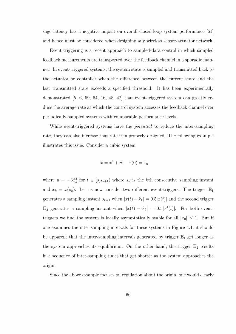
sage latency has a negative impact on overall closed-loop system performance [61]

and hence must be considered when designing any wireless sensor-actuator network.

Event triggering is a recent approach to sampled-data control in which sampled

feedback measurements are transported over the feedback channel in a sporadic man-

ner. In event-triggered systems, the system state is sampled and transmitted back to

the actuator or controller when the difference between the current state and the

last transmitted state exceeds a specified threshold. It has been experimentally

demonstrated [5, 6, 59, 64, 16, 48, 42] that event-triggered system can greatly re-

duce the average rate at which the control system accesses the feedback channel over

periodically-sampled systems with comparable performance levels.

While event-triggered systems have the potential to reduce the inter-sampling

rate, they can also increase that rate if improperly designed. The following example

illustrates this issue. Consider a cubic system

x = x3 + u; x(0) = x0

where u = −3x3k for t ∈ [s,sk+1) where sk is the kth consecutive sampling instant

and xk = x(sk). Let us now consider two different event-triggers. The trigger E1

generates a sampling instant sk+1 when |x(t)− xk| = 0.5|x(t)| and the second trigger

E2 generates a sampling instant when |x(t) − xk| = 0.5|x4(t)|. For both event-

triggers we find the system is locally asymptotically stable for all |x0| ≤ 1. But if

one examines the inter-sampling intervals for these systems in Figure 4.1, it should

be apparent that the inter-sampling intervals generated by trigger E1 get longer as

the system approaches its equilibrium. On the other hand, the trigger E2 results

in a sequence of inter-sampling times that get shorter as the system approaches the

origin.

Since the above example focuses on regulation about the origin, one would clearly

66

0 1 2 3 4 50

0.5

1

1.5

2

inte

r−sa

mpl

ing

inte

rval

:s

time:s

E

1

0 1 2 3 4 50.04

0.06

0.08

0.1

0.12

inte

r−sa

mpl

ing

inte

rval

:s

time:s

E

2

Figure 4.1. Inter-sampling intervals for two different types of event-triggers

want the inter-sampling interval to be longest when the system is close to the origin.

The ‘interesting’ feedback information that mandates use of the feedback channel

should occur when the system is perturbed away from the origin, not when the system

is resting in the neighborhood of the origin. This ”desired” behavior is exhibited by

event-trigger E1, but as shown in Figure 4.1, the opposite trend is exhibited by

event-trigger E2. Event trigger E1 is said to be efficiently attentive because the

control system is more efficient in its use of the channel when the system state is

close to the origin.

One reason why there has been such great interest in the inter-sampling interval

is that it can be taken as a measure of channel usage. Much of this prior work,

however, [59, 24, 44, 46] has ignored delays or quantization errors. For this rea-

son, results bounding the inter-sampling interval only provide a partial picture of an

event-triggered system’s network usage. Recent work has begun to consider constant

bounded delays [71, 72, 20, 33], but this chapter shows that delays preserving input-

to-state stability (ISS) are state-dependent, thereby suggesting that the ‘bit-rates’

required to support event-triggered systems are time-varying. If, in fact, one can as-

sure that these ‘instantaneous’ bit-rates are efficiently attentive, then one reduces the

average bit rate over systems using constant bounded delays. The main results in this

chapter establish sufficient conditions for an event-triggered system’s instantaneous

bit-rate to be efficiently attentive. We then provide simulation examples to illus-

67

trate the value of these results. In the examples, we also see a tradeoff between the

inter-sampling interval and the instantaneous bit-rate. This tradeoff indicates that

we should not only focus on lengthening the inter-sampling interval, but also need to

guarantee the channel bandwidth satisfies the required instantaneous bit-rate.

4.2 Notation and Background on Input-to-State Stability

4.2.1 Notation

Throughout this chapter, the n dimensional real space will be denoted as Rn

and the set of non-negative reals will be denoted as R+. The infinity (supremum)

norm of a vector x ∈ Rn will be denoted as ∥x∥. The L-infinity norm of a function

x(·) : R+ → Rn is defined as ∥x∥L∞ = ess supt≥0 ∥x(t)∥. This function is said to be

essentially bounded if ∥x∥L∞ < ∞ and the linear space of all essentially bounded

real-valued functions will be denoted as L∞. A subset Ω ⊂ Rn is said to be compact

if it is closed and bounded.

A function α(·) : R+ → R+ is class K if it is continuous, strictly increasing and

α(0) = 0. It is said to be of K∞, if α(s) → ∞ as s → ∞. A function β : R+ ×R+ →

R+ is class KL if β(·, t) is class K for each fixed t ≥ 0 and β(r, t) decreases to 0 as

t → ∞ for each fixed r ≥ 0.

Lemma 4.2.1. Let g : [0, σ] → R+ be a continuous, positive definite function satisfy-

ing lims→0 < ∞. There must exist continuous, positive definite, increasing functions

h and h defined on [0, σ] such that

h(s) ≤ g(s) ≤ h(s), ∀s ∈ [0, σ],

lims→0

g(s) = lims→0

h(s) = lims→0

h(s).

Proof. See Lemma 4.3 in [32].

68

Let Ω be a compact subset of Rn. We say f(·) : Ω → Rn is locally Lipschitz on Ω

if for any x, y ∈ Ω, there exists a constant L ≥ 0 such that

∥f(x)− f(y)∥ ≤ L∥x− y∥

4.2.2 Background on Input-to-State Stability

Consider a system whose state trajectory x(·) : R+ → Rn satisfies the initial value

problem,

x(t) = f(x(t), w(t)), x(0) = x0 (4.1)

where w(·) : [0,∞) → Rm is an essentially bounded signal. Let x = 0 be an equilib-

rium point for (4.1) with w(t) ≡ 0, and Υ ⊂ Rn be a domain containing x = 0. Let

V : Υ → R be a continuously differentiable function such that

α(∥x∥) ≤ V ≤ α(∥x∥), (4.2)

∂V

∂xf(x,w) ≤ −α(∥x∥) + γ(∥w∥), (4.3)

for all (x,w) ∈ Υ × Rm, where α, α are class K∞ functions, and α, γ are class K

functions, then the system (4.1) is input-to-state stable (ISS). The function V is

called ISS-Lyapunov function.

4.3 Problem Statement

The system under study is a wireless networked event-triggered control system

with quantization shown in Figure 4.2.

Consider the following plant whose state satisfies the following differential equa-

69

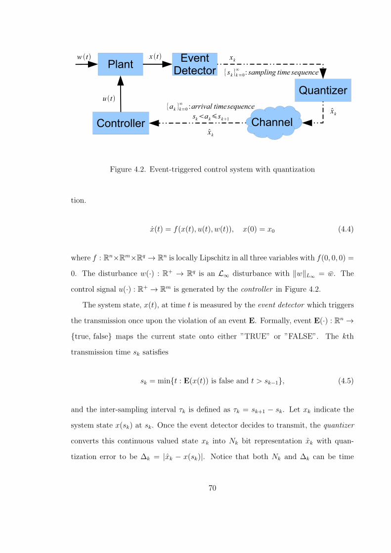
Figure 4.2. Event-triggered control system with quantization

tion.

x(t) = f(x(t), u(t), w(t)), x(0) = x0 (4.4)

where f : Rn×Rm×Rq → Rn is locally Lipschitz in all three variables with f(0, 0, 0) =

0. The disturbance w(·) : R+ → Rq is an L∞ disturbance with ∥w∥L∞ = w. The

control signal u(·) : R+ → Rm is generated by the controller in Figure 4.2.

The system state, x(t), at time t is measured by the event detector which triggers

the transmission once upon the violation of an event E. Formally, event E(·) : Rn →

true, false maps the current state onto either ”TRUE” or ”FALSE”. The kth

transmission time sk satisfies

sk = mint : E(x(t)) is false and t > sk−1, (4.5)

and the inter-sampling interval τk is defined as τk = sk+1 − sk. Let xk indicate the

system state x(sk) at sk. Once the event detector decides to transmit, the quantizer

converts this continuous valued state xk into Nk bit representation xk with quan-

tization error to be ∆k = |xk − x(sk)|. Notice that both Nk and ∆k can be time

70

varying and state dependent. The quantized state xk is, then, transmitted to the

controller with delay dk. The instantaneous bit-rate rk is, then, defined as rk = Nk

dk,

and the arrival time ak of the kth transmission, then, satisfies ak = sk + dk. We

say that the transmission and arrival sequences are admissible if sk < ak ≤ sk+1 for

k = 0, 1, . . . ,∞.

Upon the arrival of the kth quantized state, xk, at the controller, a control input

is computed and then held until the next quantized state is received. In other words,

the control signal takes the form

u(t) = uk = K(xk) (4.6)

for t ∈ [ak, ak+1). The function K(·) : Rn → Rm is locally Lipschitz, and satisfies

K(0) = 0. As has been done in [59], this chapter assumes that K is chosen so the

system

x(t) = f(x(t), K(x(t) + e(t)), w(t)), (4.7)

is locally input-to-state stable with respect to the signals e, w ∈ L∞. This means, of

course, that there exists a function V (·) : Υ → R+ satisfying

α(∥x∥) ≤ V ≤ α(∥x∥) (4.8)

∂V

∂xf(x,w) ≤ −α(∥x∥) + γ1(∥e∥) + γ2(∥w∥), (4.9)

for all x ∈ Υ where Υ ⊆ Rn is a domain containing the origin, α, α, α, γ1 and γ2 are

class K functions.

Our objective is to design the event detector and the quantizer such that the

system defined in (5.1), (4.5) and (4.6) is ISS and efficiently attentive.

Definition 4.3.1. The system defined in (5.1), (4.5) and (4.6) is said to be efficiently

71

attentive if there exists a continuous, positive definite function h(s1, s2) satisfying

lims→0 h(s1, s2) > 0 and decreasing with respect to both variables, and a continuous,

positive definite function h(s1, s2) satisfying lims→0 h(s1, s2) < ∞ and increasing with

respect to both variables such that

• the inter-sampling interval τk is bounded from below by h(∥xk−1∥, ∥xk∥), i.e.

τk ≥ h(∥xk−1∥, ∥xk∥). (4.10)

• the instantaneous bit-rate rk is bounded from above by h(∥xk−1∥, ∥xk∥), i.e.

rk ≤ h(∥xk−1∥, ∥xk∥). (4.11)

Remark 4.3.2. The bounds on τk and rk depend on both xk−1 and xk, because xk

is transmitted with some delay, and both xk−1 and xk are used to produce control

input and hence influence the system dynamic during intervals [sk, ak) and [ak, sk+1],

respectively.

Remark 4.3.3. The requirement (4.10) on τk indicates how often the event-triggered

control system uses communication resources. Once requirement (4.10) is satisfied,

the event-triggered control system will use the communication less frequently as the

system state get closer to the origin.

Remark 4.3.4. The requirement (4.11) on rk indicates how much communication

resources (i.e. bandwidth) is used by the event-triggered control system in each trans-

mission. Equation (4.11) requires the event-triggered control system uses fewer com-

munication resources as the system state gets closer to the origin.

To guarantee ISS and efficient attentiveness, we first provide the event detector

and quantizer guaranteeing ISS assuming there is no delay, then study the accept-

able delay based on the designed event detector and quantizer, and finally give the

sufficient condition of efficient attentiveness.

72

4.4 Event Detector and Quantizer Guaranteeing ISS without Delay.

Let us first look at the dynamic behavior of the closed loop system. Let ek(t) =

x(t) − xk be the gap between the current state and the kth quantized state. From

equation (4.8) and (4.9), it is easy to get the following lemma.

Lemma 4.4.1. Given the event-triggered system in (5.1-4.5) whose controller (4.6)

satisfies is locally ISS and satisfies (4.8-4.9). If for all t ∈ [ak, ak+1) and all k =

0, 1, · · · ,∞,

∥ek(t)∥ ≤ ξ(∥x(t)∥, w) = γ−11 (cα(∥x(t)∥) + γ3(w)), (4.12)

where c ∈ (0, 1) and γ3 is a K function, then the system is locally ISS.

Proof. Apply equation (4.12) into equation (4.9), we have

∂V

∂xf(x,w) ≤ −(1− c)α(∥x∥) + γ2(w) + γ3(w),∀t ≥ 0.

Since c ∈ (0, 1) and γ2(w) + γ3(w) is a class K function of w, the system is ISS.

Suppose that ξ(s, w) in (4.12) is locally Lipschitz for all s ∈ Υ with the Lipschitz

constant Lξ. Let

ξ(s, w) =1

Lξ + 1ξ(s, w). (4.13)

It can be shown that

Corollary 4.4.2. Given the event-triggered system in (5.1-4.5) whose controller (4.6)

satisfies is locally ISS and satisfies (4.8-4.9). If ∥ek(t)∥ ≤ ξk= ξ(∥xk∥, w) in (4.13) ,

for all t ∈ [ak, ak+1) and all k = 0, 1, · · · ,∞, then the event-triggered system is ISS.

73

Proof.

∥ek(t)∥ ≤ 1

Lξ + 1ξ(∥xk∥, w)

≤ 1

Lξ + 1ξ(∥x(t)∥+ ∥ek(t)∥, w).

≤ 1

Lξ + 1ξ(∥x(t)∥, w) + Lξ

Lξ + 1∥ek(t)∥

⇒ ∥ek(t)∥ ≤ ξ(∥x(t)∥, w)

According to lemma 4.4.1, the above equation implies the system is ISS.

Now, let us choose our event-trigger as

E : ∥ek(t)∥ < θk = θ(∥xk∥, w) = ρθξ(∥xk∥, w), (4.14)

where ρθ ∈ (0, 1) is a given constant. Let ∆k be the quantization error at the kth

transmission time. To make sure the inter-sampling interval is strictly positive, we

need to guarantee ∆k < θk, so ∆k is chosen as

∆k = ρ∆θ(|∥xk−1∥ − θk−1|, w), (4.15)

where ρ∆ ∈ (0, 1) is a given constant. The proof of the following Lemma 4.4.3 shows

that (4.15) implies ∆k < θk. We assume that the controller knows the event-trigger

and the quantization error. So, when the controller receives the kth packet, it knows

that the state x satisfies ∥x− xk−1∥ = θk−1. The set x : ∥x− xk−1∥ = θk−1 is then

uniformly quantized such that ∥x− xk∥ ≤ ∆k, and the number of bits Nk transmitted

at sk satisfies

Nk = ⌈log2 2n⌉+

⌈log2

⌈θk−1

∆k

⌉n−1⌉. (4.16)

74

Lemma 4.4.3. Suppose there is no delay. The system defined in (5.1-4.6) with the

event-trigger and quantization error defined as (4.14) and (4.15) is ISS.

Proof. From equation (4.12-4.14), we see that θ(s, w) is a increasing function of s.

Since ∥xk − xk−1∥ = θk−1 ⇒ ∥xk∥ ≥ |∥xk−1∥ − θk−1|, we have

∥ek(sk)∥ ≤ ∆k < θ(|∥xk−1∥ − θk−1|, w) ≤ θ(∥xk∥, w) = θk.

Since ∥ek(sk+1)∥ = θk, according to the continuity of ek, ∥ek∥ < ξkfor all t ∈ [sk, sk+1)

and all k = 0, 1, · · · ,∞. From Corollary 4.4.2, the system is ISS.

4.5 Acceptable Delays Preserving Input-to-State Stability

Corollary 4.4.2 indicates that bounding ek(t) during interval [ak, ak+1) is essential

to preserve the input-to-state stability of the closed loop system. A typical trajectory

of ∥ek(t)∥ is shown in Figure 4.3. At time sk, system state is quantized and trans-

mitted with the initial gap ∥ek(sk)∥ ≤ ∆k. This gap gradually increases and finally

hits θk, which generates the k + 1-st sampling instant. Before the k + 1-st quantized

state arrives at the controller, the gap ∥ek(t)∥ keeps increasing. To guarantee ISS,

the gap ∥ek(t)∥ should be bounded by ξk.

The gap ek(t) has the following dynamic behavior.

ek(t) = f(xk + ek(t), uk, w(t)),∀t ∈ [ak, ak+1). (4.17)

Let Lxk be the Lipschitz constant of f with respect to x during interval [sk, ak]. ∥f∥

is bounded from above by

∥f(xk + ek(t), uk, w)∥ ≤ f(xk, uk, w) + Lxk∥ek∥, (4.18)

75

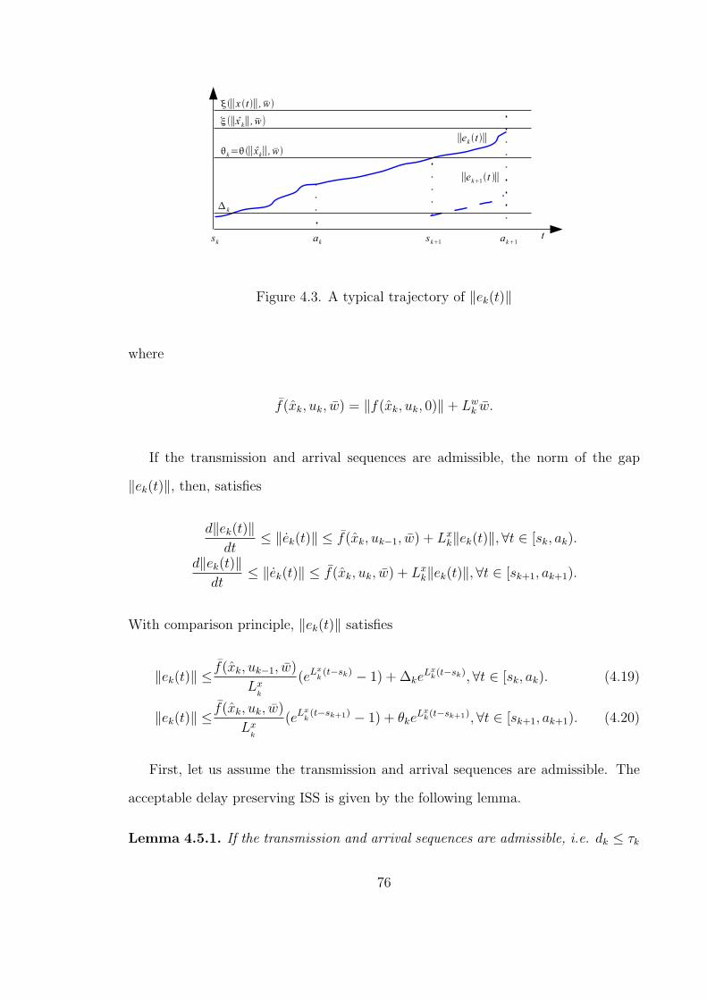
Figure 4.3. A typical trajectory of ∥ek(t)∥

where

f(xk, uk, w) = ∥f(xk, uk, 0)∥+ Lwk w.

If the transmission and arrival sequences are admissible, the norm of the gap

∥ek(t)∥, then, satisfies

d∥ek(t)∥dt

≤ ∥ek(t)∥ ≤ f(xk, uk−1, w) + Lxk∥ek(t)∥,∀t ∈ [sk, ak).

d∥ek(t)∥dt

≤ ∥ek(t)∥ ≤ f(xk, uk, w) + Lxk∥ek(t)∥,∀t ∈ [sk+1, ak+1).

With comparison principle, ∥ek(t)∥ satisfies

∥ek(t)∥ ≤ f(xk, uk−1, w)

Lxk

(eLxk(t−sk) − 1) + ∆ke

Lxk(t−sk), ∀t ∈ [sk, ak). (4.19)

∥ek(t)∥ ≤ f(xk, uk, w)

Lxk

(eLxk(t−sk+1) − 1) + θke

Lxk(t−sk+1),∀t ∈ [sk+1, ak+1). (4.20)

First, let us assume the transmission and arrival sequences are admissible. The

acceptable delay preserving ISS is given by the following lemma.

Lemma 4.5.1. If the transmission and arrival sequences are admissible, i.e. dk ≤ τk

76

for all k = 0, 1, . . . ,∞, and the transmission delay dk+1 satisfies

dk+1 ≤ dk+1 =1

Lxk

ln

(1 +

Lxk(ξk − θk)

f(xk, uk, w) + Lxkθk

), (4.21)

then the system defined in (5.1), (4.5) and (4.6) with the event-trigger and quantiza-

tion error defined as (4.14) and (4.15) is ISS.

Proof. We assume ak ≤ sk+1 ≤ ak+1 for all k = 0, 1, . . . ,∞.

It is easy to see that during interval [ak, sk+1], ∥ek(t)∥ ≤ θk < ξk.

For interval [sk+1, ak+1), from equation (4.20), we have

∥ek(t)∥ ≤ ∥ek(ak+1)∥ ≤ f(xk, uk, w)

Lxk

(eLxkdk+1 − 1) + θke

Lxkdk+1 ,∀t ∈ [sk+1, ak+1)

So, equation (4.13) is guaranteed by

f(xk, uk, w)

Lxk

(eLxkdk+1 − 1) + θke

Lxkdk+1 < ξ

k⇔ dk+1 ≤ dk+1

Therefore, ∥ek(t)∥ < ξkholds for all t ∈ [ak, ak+1) and all k = 0, 1, . . . ,∞. Ac-

cording to Corollary 4.4.2, the closed loop system is ISS.

Next, we would like to find an upper bound on the delay such that the transmission

arrival sequences are admissible.

Lemma 4.5.2. If the transmission delay dk satisfies

dk ≤ Tk =1

Lxk

ln

(1 +

Lxk(θk −∆k)

f(xk, uk−1, w) + Lxk∆k

), (4.22)

then the transmission arrival sequences are admissible, i.e. dk ≤ τk for all k =

0, 1, . . . ,∞.

Proof. First, we realize that d0 = 0 ≤ τ0.

77

Now, let us assume that dk−1 ≤ τk−1 holds, i.e. ak−1 ≤ sk. If dk > τk, then we

have ak−1 ≤ sk ≤ sk+1 < ak. For interval [sk, sk+1], from equation (4.19), we have

∥ek(sk+1)∥ ≤ f(xk, uk−1, w)

Lxk

(eLxkτk − 1) + ∆ke

Lxkτk .

Since ∥ek(sk+1)∥ = θk, together with the equation above, we have τk ≥ Tk. From

equation (4.22), we further have τk ≥ dk. This contradicts the assumption dk > τk.

Therefore, dk ≤ τk for all k = 0, 1, . . . ,∞.

Corollary 4.5.3. If dk ≤ Tk, then the inter-sampling interval τk is bounded from

below by Tk, i.e.

τk ≥ Tk, (4.23)

where Tk is defined in (4.22).

Proof. The contrapositive of Lemma 4.5.2 is

dk > τk ⇒ dk > Tk. (4.24)

Assume Tk > τk. It is easy to see that

dk > Tk ⇒ dk > τk. (4.25)

From equation (4.24) and (4.25), we have

dk > τk ⇔ dk > Tk,

which implies τk = Tk. This contradicts the assumption Tk > τk. So, τk ≥ Tk

From Lemma 4.5.1 and 4.5.2, the main theorem is obtained.

78

Theorem 4.5.4. If the transmission delay dk satisfies

dk ≤ Dk = mindk, Tk, (4.26)

where dk and Tk are given by (4.21) and (4.22) respectively, then the transmission

and arrival sequences are admissible and the system defined in (5.1-4.6) with the

event-trigger and quantization error defined as (4.14) and (4.15) is ISS.

Remark 4.5.5. Theorem 4.5.4 indicates that when transmission delays are not neg-

ligible, we should not choose θk as large as possible to obtain as large as possible

inter-sampling interval. Because as θk gets closer and closer to ξk, dk dominates the

bound on the acceptable delay, and gets smaller and smaller according to (4.21).

Remark 4.5.6. The results in Corollary 4.5.3 and Theorem 4.5.4 provide a basis

to study the scheduling problem in large scale event-triggered control systems. Let us

assume that there are several control systems which share a communication channel,

and there is a scheduler which schedules the transmissions of all the control systems.

Every time when a control system decides to transmit, from the results in Corollary

4.5.3 and Theorem 4.5.4, it tells the scheduler that Nk bits need to be transmitted

in Dk seconds, and the next transmission time will be at least Tk seconds later. The

scheduler, then, makes use of the information from all control systems to decide

whether all transmission requirements are schedulable.

This section uses the technique that we used in [64] to derive bounds on acceptable

delay and inter-sampling interval. These results are further analyzed in the next

section to explain how efficient attentiveness is achieved.

4.6 Efficient Attentiveness

This section studies the sufficient condition achieving efficient attentiveness. For

the convenience of the rest of this section, we first define fc(s) as a class K function

79

satisfying

∥f(xk, K(xk), 0)∥ ≤ fc(∥xk∥), (4.27)

and we have the following corollary which is a direct result from Lemma 4.2.1.

Corollary 4.6.1. If

lims→0

fc(s)

θ(s, 0)<∞, (4.28)

then there exist continuous, positive definite, increasing functions h1(s), h2(s) such

that lims→0 hi(s) < ∞ for i = 1, 2 and

θ(s, w)

∆(s, w)≤ h1(s) (4.29)

fc(s) + Lwk w

θ(s, w)≤ h2(s). (4.30)

Proof. If w = 0, it is easy to show that

lims→0

θ(s, w)

∆(θ(s, w))< ∞

lims→0

fc(s) + Lwk w

θ(s, w)< ∞.

According to Lemma 4.2.1, there must exist h1 and h2 which are continuous, positive

definite, increasing and lims→0 hi(s) < ∞ for i = 1, 2 such that equation (4.29) and

(4.30) hold.

If w = 0, we have

lims→0

θ(s, 0)

∆(θ(s, 0))= lim

s→0

θ(s, 0)

ρ∆θ(|s− θ(s, 0)|, 0)

From (4.12) and (4.13), we know that θ(s, 0) is a continuous function satisfying

80

θ(0, 0) = 0. There must exist a constant c such that for all s ∈ [0, c], θ(s, 0) is either

greater or equal to 0.5s, or less than 0.5s. If θ(s, 0) ≤ 0.5s, then

lims→0

θ(s, 0)

ρ∆θ(|s− θ(s, 0)|, 0)≤ lim

s→0

θ(s, 0)

ρ∆θ(0.5s, 0)< ∞.

If θ(s, 0) > 0.5s, then

lims→0

θ(s, 0)

ρ∆θ(|s− θ(s, 0)|, 0)≤ lim

θ(s,0)→0

θ(s, 0)

ρ∆θ(3θ(s), 0)<

2

3ρ∆< ∞.

Together with (4.28), according to Lemma 4.2.1, equation (4.29) and (4.30) still

hold.

4.6.1 Efficiently Attentive Inter-Sampling Interval

Now, we are ready to present a sufficient condition to achieve efficiently attentive

inter-sampling interval.

Lemma 4.6.2. If the assumption (4.28) is satisfied, then the inter-sampling interval

τk is efficiently attentive, i.e. there exists a continuous, positive definite, decreasing

function h(s1, s2) such that lims→0 h(s1, s2) > 0 and equation (4.10) is satisfied.

Proof. From Corollary 4.5.3, we have τk ≥ Tk. Since ln(1 + x) ≥ x1+x

, it is easy to

show that

Tk ≥θk −∆k

f(xk, uk−1, w) + Lxkθk

=1−∆k/θk

f(xk, uk−1, w)/θk + Lxk

.

From the proof of Lemma 4.4.3, we know that ∆k < ρ∆θk. We further have

τk ≥ Tk ≥1− ρ∆

f(xk, uk−1, w)/θk + Lxk

.

81

f is locally lipschitz with respect to xk, so

f(xk, uk−1, w)

θk≤ f(xk−1, uk−1, w) + Lx

k∥xk − xk−1∥θk

≤ fc(∥xk−1∥) + Lwk w + Lx

kθk−1

∆k

≤ fc(∥xk−1∥) + Lwk w

θk−1

θk−1

∆k

+ Lxk

θk−1

∆k

According to Corollary 4.6.1, there must exist continuous, positive definite, and in-

creasing functions h1(∥xk−1∥) and h2(∥xk−1∥) such that

f(xk, uk−1, w)

θk≤ h1(∥xk−1∥) + Lx

kh2(∥xk−1∥),

and hence we have

τk ≥ Tk ≥1− c1

h1(∥xk−1∥) + Lxkh2(∥xk−1∥) + Lx

k

.

Since h1 and h2 are increasing with respect to ∥xk−1∥, Lxk is increasing with respect

to ∥xk∥, and h1, h2 and Lxk are all bounded from above as x approaches 0, we say

that there exists a continuous, positive definite, decreasing function h(∥xk−1∥, ∥xk∥)

such that lim∥xk−1∥,∥xk∥→0 h(∥xk−1∥, ∥xk∥) > 0, and equation (4.10) is satisfied.

4.6.2 Efficiently Attentive Instantaneous Bit-Rate

Since the instantaneous bit-rate rk is defined as Nk/Dk, it is easy to see that the

instantaneous bit-rate rk is efficiently attentive if Nk is bounded from above by an

increasing function, and Dk is bounded from below by a decreasing function. Both

Nk and Dk will be studied in this subsection.

First, let us look at the number of bits Nk transmitted at step k.

Lemma 4.6.3. There exists a continuous, positive definite increasing function h′(∥xk−1∥)

82

such that

lims→0

h′(s) < ∞ (4.31)

Nk ≤ h′(∥xk−1∥). (4.32)

Proof. Nk satisfies

Nk = ⌈log2 2n⌉+

⌈log2

⌈θk−1

∆k

⌉n−1⌉.

According to Corollary 4.6.1, there exists a continuous, positive definite, increasing

function h1(∥xk−1∥) such that

lims→0

h1(s) < ∞

θk−1

∆k

≤ h1(∥xk−1∥).

Therefore, there must exist a continuous, positive definite increasing function h′(∥xk−1∥)

such that equation (4.31) and (4.32) hold.

Next, we would like to study Dk. Since Dk = minTk, dk and Tk has be analyzed

in Lemma 4.6.2, only dk is examined here.

Lemma 4.6.4. If the assumption (4.28) is satisfied, then there exists a continuous,

positive definite decreasing function h′′(∥xk−1∥, ∥xk∥) such that

lims1,s2→0

h′′(s1, s2) > 0 (4.33)

dk ≥ h′′(∥xk−1∥, ∥xk∥). (4.34)

Proof. Since θk = ρθξk, with the same steps in the proof of Lemma 4.6.2, we show

83

that

dk ≥1− ρθ

f(xk−1, uk−1, w)/ξk + Lxk

,

where

f(xk−1, uk−1, w)

ξk

≤ fc(∥xk−1∥) + Lwk w

θk−1

.

According to Corollary 4.6.1, there exist a continuous, positive definite, increasing

function h2(∥xk−1∥) such that

lims→0

h2(s) <∞,

f(xk−1, uk−1, w)

ξk

≤h2(∥xk−1∥).

Together with the fact that Lxk is increasing with respect to ∥xk∥ and limx → 0Lx

k <

∞, we conclude that there exists a continuous, positive definite decreasing function

h′′(s1, s2) such that equation (4.33) and (4.34) hold.

From Lemma 4.6.2, 4.6.3 and 4.6.4, we have the following corollary.

Corollary 4.6.5. If equation (4.28) are satisfied, the instantaneous bit-rate rk is ef-

ficiently attentive, i.e. there exists a continuous, positive definite, increasing function

h(s1, s2) such that lims→0 h(s1, s2) < ∞ and equation (4.11) is satisfied.

4.6.3 Efficiently Attentive and ISS Event Triggered Control System

Now, we are at the step to make a conclusion. Event triggered control systems

should be designed to achieve not only a desired system performance but also atten-

tion efficiency. To this purpose, we have the following theorem which is easily derived

from Theorem 4.5.4, Lemma 4.6.2, and Corollary 4.6.5.

84

Theorem 4.6.6. If the transmission delay dk is bounded from above by Dk given by

(4.26), and the threshold function θ satisfy equation (4.28), then the system defined

in (5.1-4.6) with the event-trigger and quantization error defined as (4.14) and (4.15)

is input-to-state stable and efficiently attentive.

Remark 4.6.7. Equation (4.28) indicates that as the system state approaches 0, the

threshold function θ decreases more slowly than the closed loop dynamic behavior of

the state trajectory. Therefore, when x get closer to 0, it takes more time for the gap

ek(t) to hit the threshold θk and ξk, which leads to longer inter-sampling interval and

acceptable delay.

4.7 A Case Study

This section uses an example to explain how to design an event-triggered control

system to achieve ISS and attention efficiency. After the event-triggered control

system is well established, we will try different threshold functions to study the

tradeoff between the inter-sampling interval and the instantaneous bit-rate.

Our experiment shows that the threshold function should be chosen as large as

possible while the instantaneous bit-rate is lower than the channel capacity. It is

also found that the event-triggered control system with its threshold function to be

0.6ξ can tolerate 25 times of the delay tolerated by the system with the threshold

function to be 0.99ξ, while only transmitting 2 times as frequently as the system with

the threshold function to be 0.99ξ.

85

4.7.1 Design of event-triggered control systems

Consider the following nonlinear dynamic system.

x1 =− 2x31 + x3

2 + w1 (4.35)

x2 =x32 + u+ w2, (4.36)

with x0 = [1 1]T . w is an L∞ disturbance with ∥w∥L∞ = 0.1. The control input u is

chosen such that

uk = −3x32, ∀t ∈ [ak, ak+1).

First, the input-to-state stability is studied for the dynamic system described in

equation (4.35) and (4.36). Let V = 14x41 +

14x42 be a Lyapunov candidate function.

Its derivative satisfies

V = −2x61 + x3

1x32 − 2x6

2 + x31w1 + x3

2w2 + 3(3x22e2 − 3x2e

22 + e32)x

32,

where ei = xi(t)− xi(sk) for i = 1, 2. Let Ω = x : ∥x∥ ≤ 1.

V ≤ −1.5x61 − 1.5x6

2 + 2w + 3x32(3x

22e2 − 3x2e

22 + e33),∀x ∈ Ω.

If

∥e∥ ≤ ϵ∥x∥l + w, for all l ≥ 1,

86

we have

V ≤− 1.5x61 − 1.5x6

2 + 2w + 3(3ϵ+ 3ϵ2 + ϵ3)∥x∥6

+ 3∥x∥5w − 6ϵ∥x∥5w − 3∥x∥4w2 + 3ϵ2∥x∥5w + 3ϵ∥x∥4w2 + ∥x∥3w3

≤− 1.5x61 − 1.5x6

2 + 3(3ϵ+ 3ϵ2 + ϵ3)∥x∥6

+ 3(w3 + 3|ϵ− 1|w2 + 3|ϵ− 1|2w) + 2w, ∀x ∈ Ω.

Let ϵ = 0.14, and γ(w) = 3(w3 + 3|ϵ− 1|w2 + 3|ϵ− 1|2w) + 2w. We have

V ≤ −0.055∥x∥6 + γ(w).

Therefore, the system is input-to-state stable if

∥ek(t)∥ ≤ ξ(∥x(t)∥) = 0.14∥x(t)∥l + w, for all l ≥ 1. (4.37)

According to equation (4.13), (4.14) and (4.15), we have

θ(∥xk∥) = ρθ(0.12∥xk∥l + 0.87w), for some ρθ ∈ (0, 1). (4.38)

∆(s) = ρ∆ρθ(0.12(s− θ(s))l + 0.87w), for some ρ∆ ∈ (0, 1).

4.7.2 Efficient attentiveness

This subsection will design an experiment to demonstrate Theorem 4.6.6. Ac-

cording to this theorem, if l ≤ 3, then the system is efficiently attentive. So, in this

experiment, we will fix ρθ = 0.6 and ρ∆ = 0.6, vary l = 1, 4, and run the system for

50 seconds to see how inter-sampling interval and instantaneous bit-rate change.

When w = 0, the system performance, inter-sampling interval, and instantaneous

87

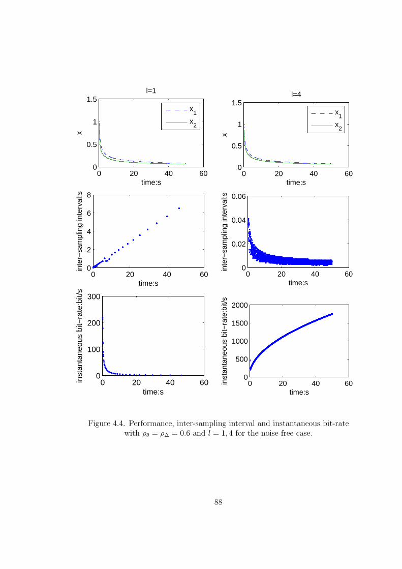
0 20 40 600

0.5

1

1.5

x

time:s

l=1

x

1

x2

0 20 40 600

0.5

1

1.5

x

time:s

l=4

x

1

x2

0 20 40 600

2

4

6

8

inte

r−sa

mpl

ing

inte

rval

:s

time:s0 20 40 60

0

0.02

0.04

0.06

inte

r−sa

mpl

ing

inte

rval

:s

time:s

0 20 40 600

100

200

300

inst

anta

neou

s bi

t−ra

te:b

it/s

time:s0 20 40 60

0

500

1000

1500

2000

inst

anta

neou

s bi

t−ra

te:b

it/s

time:s

Figure 4.4. Performance, inter-sampling interval and instantaneous bit-ratewith ρθ = ρ∆ = 0.6 and l = 1, 4 for the noise free case.

88

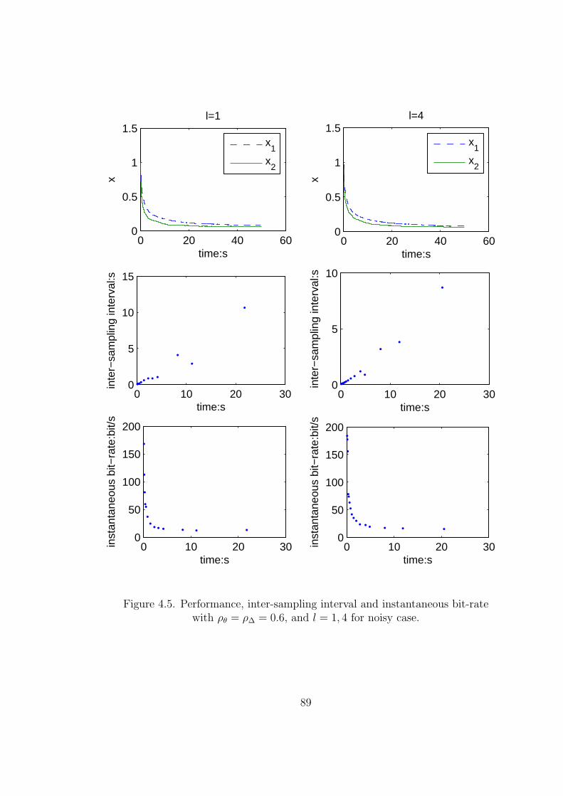
0 20 40 600

0.5

1

1.5

x

time:s

l=1

x

1

x2

0 20 40 600

0.5

1

1.5

x

time:s

l=4

x

1

x2

0 10 20 300

5

10

15

inte

r−sa

mpl

ing

inte

rval

:s

time:s0 10 20 30

0

5

10

inte

r−sa

mpl

ing

inte

rval

:s

time:s

0 10 20 300

50

100

150

200

inst

anta

neou

s bi

t−ra

te:b

it/s

time:s0 10 20 30

0

50

100

150

200

inst

anta

neou

s bi

t−ra

te:b

it/s

time:s

Figure 4.5. Performance, inter-sampling interval and instantaneous bit-ratewith ρθ = ρ∆ = 0.6, and l = 1, 4 for noisy case.

89

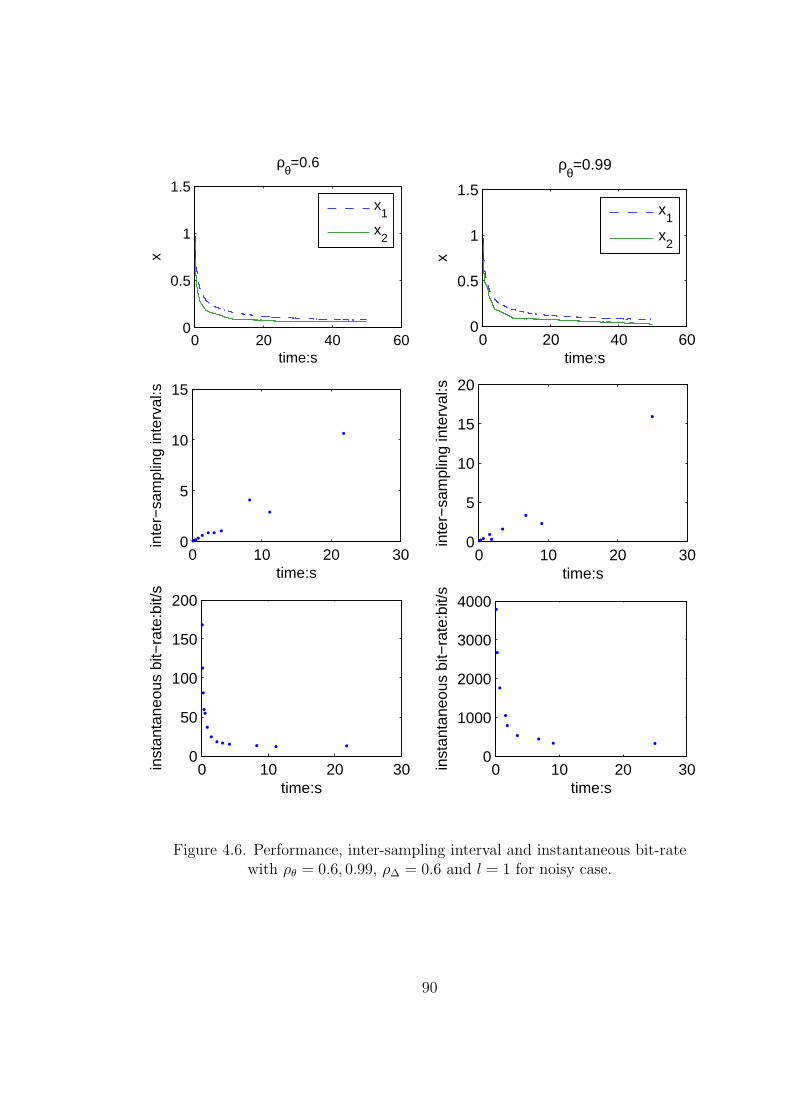
0 20 40 600

0.5

1

1.5

x

time:s

ρθ=0.6

x

1

x2

0 20 40 600

0.5

1

1.5

x

time:s

ρθ=0.99

x

1

x2

0 10 20 300

5

10

15

inte

r−sa

mpl

ing

inte

rval

:s

time:s0 10 20 30

0

5

10

15

20

inte

r−sa

mpl

ing

inte

rval

:s

time:s

0 10 20 300

50

100

150

200

inst

anta

neou

s bi

t−ra

te:b

it/s

time:s0 10 20 30

0

1000

2000

3000

4000

inst

anta

neou

s bi

t−ra

te:b

it/s

time:s

Figure 4.6. Performance, inter-sampling interval and instantaneous bit-ratewith ρθ = 0.6, 0.99, ρ∆ = 0.6 and l = 1 for noisy case.

90

bit-rate are shown in Figure 4.4. The left plots are the simulation results for l = 1.

The top plot gives the system performance, and the system is asymptotically stable.

The middle plot shows the inter-sampling interval which got longer and longer as the

system state approached 0. The bottom plot shows the instantaneous bit-rate which

was smaller and smaller as the state went to 0. So, we say the system is efficiently

attentive. The right plots are the simulation results for l = 4. We see that the

system is still ISS, but the inter-sampling interval became shorter and shorter and

the instantaneous bit-rate got larger and larger as the system state went to the origin.

Therefore, when l = 4, the system is not efficiently attentive.

When w = 0.1, the system performance, inter-sampling interval, and instanta-

neous bit-rate are shown in Figure 4.5. Comparing the left plots (l = 1) with the

right plots(l = 4), we find that for both cases, the systems had similar system per-

formances, inter-sampling intervals, and instantaneous bit-rates, and both are ISS

and efficiently attentive. This is because when w = 0, and x is small, for both cases,

the term associated with w dominated the threshold and the quantization error, and

hence for both cases, the systems had similar performances, inter-sampling intervals,

and instantaneous bit-rates.

4.7.3 The inter-sampling interval and the instantaneous bit-rate

In this section, we will fix l = 1 and ρ∆ = 0.6. By varying ρθ = 0.6, 0.99, we want

to explore the tradeoff between the inter-sampling interval and the instantaneous

bit-rate. The simulation results are shown in Figure 4.6. The left plots are the

results for ρθ = 0.6, and the right plots are the results for ρθ = 0.99. The top

plots give the system performance. we see that both of them are ISS. The middle

plots show the inter-sampling intervals. We see that the inter-sampling interval of

the system with ρθ = 0.99 is about 2 times of the inter-sampling interval of the

system with ρθ = 0.6. The bottom plots show the instantaneous bit-rates. we find

91

that the instantaneous bit-rate of the system with ρθ = 0.99 is about 20 times of

the instantaneous bit-rate of the system with ρθ = 0.6. This experiment showed

the tradeoff between inter-sampling interval and instantaneous bit-rate. When we

increased the threshold, while the inter-sampling interval increased, the required

instantaneous bit-rate also increased. Therefore, for bandwidth limited systems, we

should not only focus on lengthening the inter-sampling interval, but also need to

guarantee the channel bandwidth satisfies the required instantaneous bit-rate.

4.8 Conclusion

This chapter studies the input-to-state stability and efficient attentiveness for

bandwidth limited event-triggered control systems. A system is said to be efficiently

attentive, if the inter-sampling interval gets longer and the required instantaneous bit-

rate gets smaller when the system state goes to the origin. We first talk about how to

design the event-trigger and the quantization map, then provide the acceptable delay

preserving ISS, and finally gives a sufficient condition of efficient attentiveness. Our

simulation results demonstrated these main results, and indicates that for bandwidth

limited systems, we should not only focus on lengthening the inter-sampling interval,

but also need to guarantee the channel bandwidth satisfies the required instantaneous

bit-rate.

92

CHAPTER 5

RESILIENT EVENT TRIGGERED SYSTEMS WITH LIMITED

TRANSMISSION FREQUENCY AND INSTANTANEOUS BIT-RATE

Chapter 4 shows that if the event trigger is properly designed, the inter-sampling

interval is longer and longer as the system state approaches the origin. From the

simulation results, we see that for a cubic system, the inter-sampling interval is even

longer than 10 seconds, when the system state is close to 0. Such a long inter-

sampling interval raises a concern about resilience of event triggered systems. By

‘resilience’, we mean the system maintains state awareness and an accepted level of

operational normalcy in response to unexpected disturbances. This chapter examines

the bit-rates needed to realize event-triggered systems that are resilient to transient

faults. Using techniques from dynamically quantized control, we derive sufficient

resilient bit-rates for nonlinear scalar systems with affine controls and disturbances.

The results in this chapter suggest that, at least for transient faults, resilient control

is indeed achievable using event-triggered feedback.

5.1 Introduction

Resilient operation of critical systems is of great societal importance. Failures of

critical civil infrastructure, such as the power grid or transportation network, will

result in economic losses and societal disruptions. The scale of these disruptions

will grow larger and larger as more systems are integrated over public networks.

These public systems also become more vulnerable to malicious attacks as system

93

size increases. It is therefore crucial that the control strategies used for these systems

be resilient to these threats.

A resilient control system is one that maintains state awareness of threats and

anomalies [56]. In particular, we expect such control systems to provide guarantees

on a system’s return to operational normalcy in the presence of disturbances gener-

ated by such threats and anomalies. The impact of such threats can be modeled as

stop faults which change the structure of the system [73]. Such threats may also be

modeled as transient faults that result in a discontinuous step change in the plant’s

state. This chapter examines resilience to such transient faults. We consider a non-

linear scalar system whose operation can be divided into a safe and an unsafe regime.

The safe operating regime is an interval of time over which the controller ensures a

pre-specified performance objective. Disturbances due to threats are impulses of un-

known magnitude that may drive a system into its unsafe regime. Within the unsafe

regime it is no longer possible to guarantee system performance levels. One may, how-

ever, be able to use an emergency control action that guarantees the system’s return

to the safe regime in finite time. The main result of this chapter characterizes lower

bounds on those bit rates ensuring resilient operation of quantized event-triggered

control systems.

Event triggered systems have shown their potential to conserve communication

resources while preserving system performance. Many embedded system engineers,

however, favor the use of time-triggered over event-triggered control architectures. A

major objection to the use of event-triggered control is that it tends to generate spo-

radic information streams. In these sporadic streams, the time between consecutive

transmissions changes in a time-varying manner. This lack of predictability is seen as

an obstacle to resilient operation. This concern may appear valid on the surface, but

in fact event-triggered systems do provide some degree of predictability in that the

minimum time between successive transmissions is usually bounded away from zero.

94

In this regard, event-triggering can be seen as providing a minimum level of feedback

connectivity, with additional information being transmitted over the channel when

the system is driven away from its equilibrium point. A key question is how small

this feedback information rate can be made while still assuring resilient operation?

The main results in this chapter characterize an upper bound on the minimum bit-

rates required for resilient behavior. These results are obtained for scalar nonlinear

systems whose control and disturbance enter in an affine manner. The control input,

u, is an impulse train whose impulses are applied when sensor data is transmitted

over a communication channel to the system’s actuator. Disturbance inputs are also

impulses that force a jump in the plant’s state as the result of some transient fault.

We assume that the magnitude of these faults is unknown. The occurrence of such

a fault forces the system out of its safe operating regime and into an unsafe regime.

The main result of this chapter establishes upper bounds on the information bit rate

between sensor and actuator required to 1) eventually force an unsafe system back

into its safe operating regime and 2) maintain a specified performance level within

the safe regime.

5.2 System Setup

The system structure is shown as in Figure 5.1. The plant is a nonlinear scalar

system whose state trajectory x : R+ → R satisfies the following initial value problem,

x(t) = f(x(t)) + u(t) + w(t) (5.1)

for all t ≥ 0 with x(0) = x0. We assume that f(·) : R → R is locally Lipschitz about

the origin with Lipschitz constant L with f(0) = 0. The input signal u is a train of

control impulses and the input signal w is a train of exogenous disturbance impulses

generated by transient system faults.

95

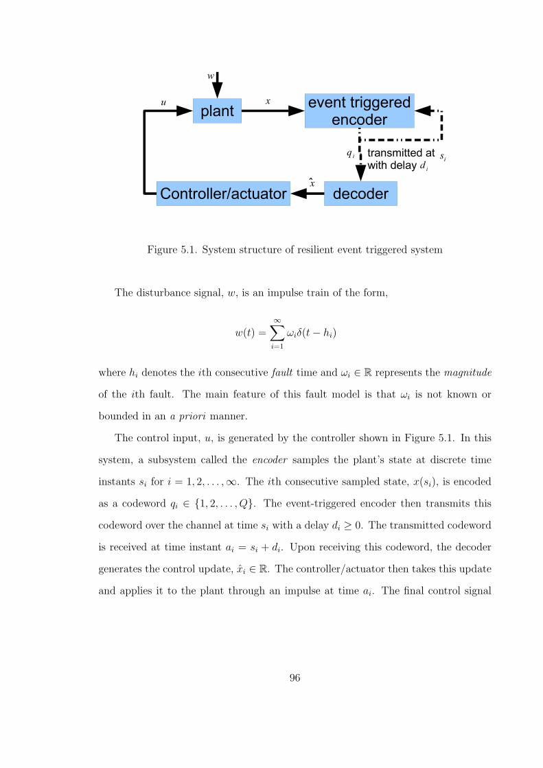
Figure 5.1. System structure of resilient event triggered system

The disturbance signal, w, is an impulse train of the form,

w(t) =∞∑i=1

ωiδ(t− hi)

where hi denotes the ith consecutive fault time and ωi ∈ R represents the magnitude

of the ith fault. The main feature of this fault model is that ωi is not known or

bounded in an a priori manner.

The control input, u, is generated by the controller shown in Figure 5.1. In this

system, a subsystem called the encoder samples the plant’s state at discrete time

instants si for i = 1, 2, . . . ,∞. The ith consecutive sampled state, x(si), is encoded

as a codeword qi ∈ 1, 2, . . . , Q. The event-triggered encoder then transmits this

codeword over the channel at time si with a delay di ≥ 0. The transmitted codeword

is received at time instant ai = si + di. Upon receiving this codeword, the decoder

generates the control update, xi ∈ R. The controller/actuator then takes this update

and applies it to the plant through an impulse at time ai. The final control signal

96

input therefore takes the form of an impulse train,

u(t) = −∞∑i=1

xiδ(t− ai)

where xi is the ith consecutive control command applied at time instant ai.

It will be convenient to restrict the system function, f , so that

f(−x) = −f(x) for all x ∈ R, (5.2)

f(|x|) is class K (5.3)

The second assumption can be relaxed at the cost of degrading the bit-rate bounds

derived below. Finally, we assume there exists a real number xa such that for all

|x| > xa we can uniformly bound |f(x)|. In other words, we assume there exist

positive constants L and L such that

|f(x)| ≤

L|x| if |x| ≤ xa

L if |x| > xa

(5.4)

We refer to the set Ωa ≡ x ∈ R : |x| ≤ xa as the absorbing region. The motivation

for this terminology is as follows. For the absorbing region, the Lipschitz constant,

L, provides an accurate upper bound on the system’s rate of growth. Outside of this

region, however, this Lipschitz approximation is too conservative because the plant’s

open-loop rate of change begins to saturate due to physical limitations within the

system.

The safe regime is a regime under which a desired level of performance is guar-

anteed (as shown in the right part of Figure 5.2). In this chapter, we specify this

desired performance as exponential stability. Let t0 be the initial time when the sys-

tem switches to the safe regime, and tf be the terminal time when the system exits

97

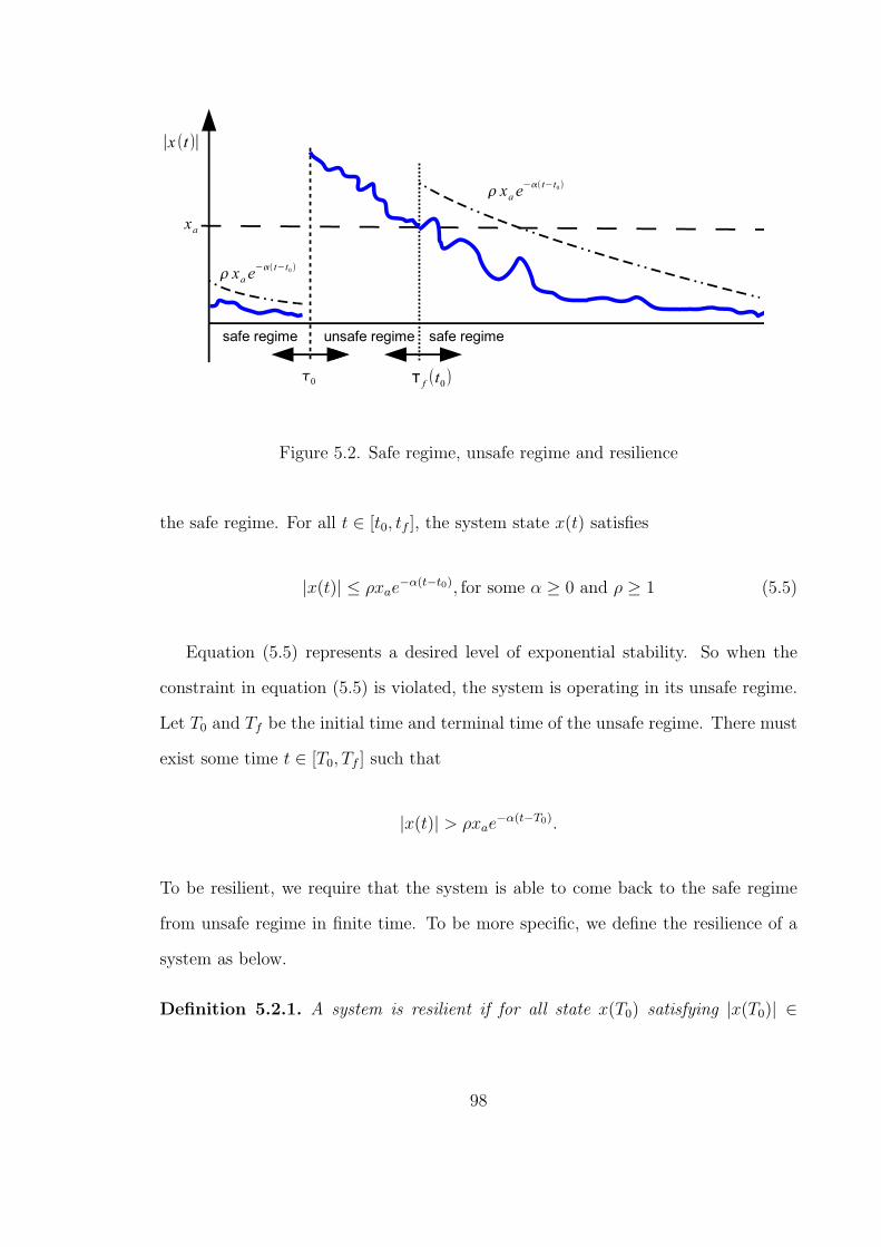
Figure 5.2. Safe regime, unsafe regime and resilience

the safe regime. For all t ∈ [t0, tf ], the system state x(t) satisfies

|x(t)| ≤ ρxae−α(t−t0), for some α ≥ 0 and ρ ≥ 1 (5.5)

Equation (5.5) represents a desired level of exponential stability. So when the

constraint in equation (5.5) is violated, the system is operating in its unsafe regime.

Let T0 and Tf be the initial time and terminal time of the unsafe regime. There must

exist some time t ∈ [T0, Tf ] such that

|x(t)| > ρxae−α(t−T0).

To be resilient, we require that the system is able to come back to the safe regime

from unsafe regime in finite time. To be more specific, we define the resilience of a

system as below.

Definition 5.2.1. A system is resilient if for all state x(T0) satisfying |x(T0)| ∈

98

(xa,∞), there is a finite time Tf ∈ (0,∞) such that

|x(Tf )| ≤ xa. (5.6)

We use the term resilience to refer to a system’s ability to return to the safe regime

in finite time. What makes resilience distinct from robustness is that the transient

faults have an arbitrarily large magnitude, rather than just a bounded magnitude.

Because the magnitude of the fault can be arbitrarily large, the controller/actuator

doesn’t know exactly what control level is needed to return the state to the origin.

So we propose having the controller apply an emergency or unsafe control step. The

main result of this chapter characterizes the rate at which this emergency control

must be applied to assure that the system is resilient; i.e. that it returns to its safe

regime in finite time.

5.2.1 Necessary Bit-Rate under Safe Regime

Let’s assume that at time t0, the system enters the safe regime. Define ϕ(x0, t−t0)

as the zero-input behavior of plant (5.1), where x0 and t0 are the initial state and

initial time. With the assumptions in (5.2) and (5.3), the zero-input behavior of plant

(5.1) has some nice properties which are given in the following lemma.

Lemma 5.2.2. If equations (5.2) and (5.3) hold, then for some small enough time

interval ϵ > 0, we have

ϕ(−x, ϵ) = −ϕ(x, ϵ), (5.7)

ϕ(x1, ϵ) ≥ ϕ(x2, ϵ), if x1 ≥ x2 ≥ 0. (5.8)

This lemma can be easily justified by noticing that for a small enough time interval

99

ϵ > 0, the state at time t+ ϵ is

ϕ(x(t), ϵ) = x(t) +

∫ t+ϵ

t

f(x(τ))dτ + o = x(t) + f(x(t))ϵ+ o,

where o indicates a negligible bias.

Next theorem gives us the necessary bit-rate to maintain exponential stability

under safe regime. The basic idea is similar to the idea used in dynamic quantization

area [69, 60].

Theorem 5.2.3. Let t0 be the initial time when the system enters its safe regime,

and β(t) = ρxae−α(t−t0). If the performance level in equation (5.5) is guaranteed for

all t ≥ t0, then the instantaneous bit-rate r(t) at time t satisfies

r(t) ≥ rs(t) = max

1

ln 2

(f(β(t))

β(t)+ α

), 0

. (5.9)

rs is called the necessary stabilizing bit-rate under safe regime.

Proof. Since performance level (5.5) is guaranteed for any t ≥ t0, we know that

for any t, x(t) is within interval [−β(t), β(t)]. From Lemma 5.2.2, we know that

after a small enough time interval ϵ, x(t + ϵ) should lie in another interval R =

[−ϕ(β(t), ϵ) + µ, ϕ(β(t), ϵ) + µ], where µ is the total amount of control input applied

during interval [t, t+ ϵ]. So the volume of R is

V (R) = 2ϕ(β(t), ϵ). (5.10)

We divide the interval R into N parts, and let Lj indicate the jth part. so the total

volume of these parts satisfies

N∑j=1

V (Lj) = V (R). (5.11)

100

By dividing R into N subintervals, the encoder determines which subinterval the

current state rests in and assigns a unique codeword to that interval. So N represents

the total number of codewords used to encode the sampled state.

Since the performance level (5.5) is guaranteed for all t ≥ t0, we know that

V (Lj) ≤ 2β(t+ ϵ). (5.12)

Therefore, from equation (5.10), (5.11) and (5.12), we arrive at the inequality that

N ≥ ϕ(β(t), ϵ)

β(t+ ϵ).

The above inequality means we need at least log2

(ϕ(β(t),ϵ)β(t+ϵ)

)bits to represent the

codeword for the sampled state. This means that the average bit-rate during this

interval is

r(t, t+ ϵ) ≥log2

(ϕ(β(t),ϵ)β(t+ϵ)

)ϵ

.

To obtain the instantaneous bit-rate at time t, we let ϵ to be infinitely close to 0, i.e.

r(t) = limϵ→0

r(t, t+ ϵ) ≥ 1

ln 2

(f(β(t))

β(t)+ α

).

Since r(t) is always non-negative, we have equation (5.9).

Remark 5.2.4. The term f(β(t))β(t)

in equation (5.9) is proportional to the fastest in-

creasing speed of the system. Our necessary stabilizing bit-rate is proportional to this

speed.

Theorem 5.2.3 is then applied to linear systems, and we have the following corol-

lary.

101

Corollary 5.2.5. If the plant (5.1) is linear, then the necessary bit-rate rs to main-

tain the performance level (5.5) under safe regime is L+αln 2

, i.e.

rs =L+ α

ln 2. (5.13)

Remark 5.2.6. The necessary bit-rate of continuous system given in [27] is recovered

by our result in equation (5.13) with α = 0, since [27] only considered uniform

boundedness.

5.2.2 Sufficient Bit-Rate under Safe Regime

This section first proposes an event triggered encoding and decoding algorithm

under safe regime, and then analyze the bit-rate of this algorithm. Finally, we would

like to discuss how to choose the parameters to achieve the necessary bit-rates for

linear systems.

Before giving the algorithm, we would like to introduce some variables to make the

algorithm easier to read. Let Me and Md, stored in encoder and decoder respectively,

indicate which regime the system is running in. To be more specific,

Me,Md =

0, under safe regime;

1, under unsafe regime,

The algorithm presented using a programmable timer whose variable, t, is reset by

the program and updated in real-time

We’re assuming the encoder and decoder both know what the triggering event

is. With this assumption, once a sampling event is triggered, then both encoder and

decoder know the magnitude of the sampled state. So, one only needs to transmit

a single bit to indicate the sign of the state. The details of this algorithm are given

below.

102

Algorithm 5.2.7. Event triggered encoding and decoding under safe regime.

Encoder algorithm

If system enters safe regime, i.e. Me = 0 and |x(t)| ≤ xa, then

1. Initialization

• Update system regime to be safe, i.e. Me = 0.

• set timer variable, t ≡ 0, and start the timer.

• Quantize x(0) as q =

00, if x(0) ≥ 0;01, if x(0) < 0.

• Send q0 to decoder.

• Wait for the acknowledgement from the decoder and set d0 = t.

2. while (t > d0)

• If |x(t)| = θ(xa, t− d0) = xae−α(t−d0),

– Quantize x(t) as q =

0, if x(t) ≥ 0;1, if x(t) < 0.

– Send q to decoder.

• If system enters unsafe regime, go to encoder algorithm under unsafe regime

Decoder algorithm

If system enters safe regime, i.e. q = 00 or 01, then

1. Initialization

• Update system regime to be safe, i.e. Md = 0.

• Reset timer variable t ≡ 0 and restart the timer.

• Estimate state as x(0) =

xa

2, if q = 00;

−xa

2, if q = 01.

• Send an acknowledgement to encoder.

2. while (Md = 0),

• If received packet is quantized data then update state estimate,

x(t) =

θ(xa, t), if q = 0;−θ(xa, t), if q = 1.

• If received packet signals regime change, then go to unsafe regime decoderalgorithm.

103

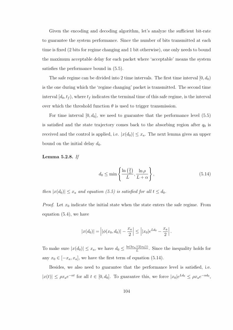
Given the encoding and decoding algorithm, let’s analyze the sufficient bit-rate

to guarantee the system performance. Since the number of bits transmitted at each

time is fixed (2 bits for regime changing and 1 bit otherwise), one only needs to bound

the maximum acceptable delay for each packet where ‘acceptable’ means the system

satisfies the performance bound in (5.5).

The safe regime can be divided into 2 time intervals. The first time interval [0, d0)

is the one during which the ‘regime changing’ packet is transmitted. The second time

interval [d0, tf ), where tf indicates the terminal time of this safe regime, is the interval

over which the threshold function θ is used to trigger transmission.

For time interval [0, d0], we need to guarantee that the performance level (5.5)

is satisfied and the state trajectory comes back to the absorbing region after q0 is

received and the control is applied, i.e. |x(d0)| ≤ xa. The next lemma gives an upper

bound on the initial delay d0.

Lemma 5.2.8. If

d0 ≤ min

ln(32

)L

,ln ρ

L+ α

, (5.14)

then |x(d0)| ≤ xa and equation (5.5) is satisfied for all t ≤ d0.

Proof. Let x0 indicate the initial state when the state enters the safe regime. From

equation (5.4), we have

|x(d0)| =∣∣∣|ϕ(x0, d0)| −

xa

2

∣∣∣ ≤ ∣∣∣|x0|eLd0 −xa

2

∣∣∣ .To make sure |x(d0)| ≤ xa, we have d0 ≤ ln(3xa/(2|x0|))

L. Since the inequality holds for

any x0 ∈ [−xa, xa], we have the first term of equation (5.14).

Besides, we also need to guarantee that the performance level is satisfied, i.e.

|x(t)| ≤ ρxae−αt for all t ∈ [0, d0]. To guarantee this, we force |x0|eLd0 ≤ ρxae

−αd0 ,

104

and have the following solution d0 ≤ ln(ρxa/|x0|)L+α

. To make sure that the inequality

holds for any |x0| ≤ xa, we have the second term of equation (5.14).

With the upper bound on the initial delay given by Lemma 5.2.8, we assure that

the system state is bounded by the threshold θ at time d0. For the second time interval

[d0, tf ), we require not only that the state is bounded by the threshold function after

packet is received and the control input is applied, i.e. |x(ai)| ≤ θ(xa, ai − d0),

but also that the performance level indicated by equation (5.5) is guaranteed, i.e

|x(t)| ≤ β(xa, t) for all t ∈ [si, ai]. To do that, we provide an upper bound on the

delay di in the next lemma.

Lemma 5.2.9. During time interval [d0, tf ), if

di ≤ min

ln 2

L+ α,ln(ρe−αd0)

L+ α

, (5.15)

where ρ satisfies ρe−αd0 > 1 for any d0 satisfies (5.14), then |x(ai)| ≤ θ(xa, ai − d0)

and |x(t)| ≤ β(xa, t) for all t ∈ [si, ai].

Proof. Using the same technique as in the proof of Lemma 5.2.8, we have

|x(ai)| ≤ |x(si)|eLdi − xae−α(si−d0+di).

To make sure |x(ai)| ≤ θ(xa, ai− d0), and realizing that |x(si)| = xae−α(si−d0), we get

di ≤ ln 2L+α

.

To guarantee |x(t)| ≤ ρxae−αt for all t ∈ [si, ai], we first notice that |x(t)| ≤

|x(si)|eLdi for all t ∈ [si, ai]. If

|x(si)|eLdi ≤ ρxae−α(si+di),

then |x(t)| ≤ β(xa, t). Solving the equation above with |x(si)| = xae−α(si−d0), we

105

have di ≤ ln(ρe−αd0 )L+α

.

Remark 5.2.10. The requirement on ρ, i.e. ρe−αd0 > 1, indicates that after time

d0, the threshold function is always below the performance level.

From Lemma 5.2.9, we see that if we properly choose parameter ρ, we can min-

imize the sufficient stabilizing bit-rate. The next corollary tells us what we should

pick.

Corollary 5.2.11. Suppose the ith transmission occurs during the time interval

[d0, tf ). If we choose ρ such that

ρ ≤ 2α+LL ,

then as long as the delay satisfies

di ≤ln 2

L+ α,

|x(ai)| ≤ θ(xa, ai − d0) and |x(t)| ≤ β(xa, t) for all t ∈ [si, ai].

Proof. This corollary is true, if ln 2L+α

≤ ln(ρe−αd0 )L+α

, i.e. d0 ≤ ln ρ2

α. To make sure that

the initial delay in (5.14) still works, we forceln ρ

2

α≥ ln ρ

L+α, and have ρ ≤ 2

α+LL .

Using Lemma 5.2.8 and corollary 5.2.11, one obtains the following theorem char-

acterizing the sufficient stabilizing bit-rate under the safe regime.

Theorem 5.2.12. Under safe regime, if q0 is transmitted with bit-rate r(0) satisfying

r(0) ≥ rs(0) =2

min

ln( 3

2)L

, ln ρL+α

,

106

and qi for i = 1, 2, · · · is transmitted with bit-rate r(i) satisfying

r(i) ≥ rs(i) =L+ α

ln 2,

then the performance level (5.5) is guaranteed with ρ ≥ 2α+LL .

Remark 5.2.13. If the system is nonlinear, it’s easy to verify that rs ≤ rs. If the

system is linear, the equality holds, i.e. rs = rs. Therefore, for linear system, we

can say that after the initial delay, the performance level (5.5) is guaranteed with the

necessary stabilizing bit-rate under safe regime.

5.3 Sufficient Bit-Rate under Unsafe Regime

This section first proposes an algorithm for unsafe regime to assure the resilience,

and then analyzes the bit-rate of this algorithm.

The basic idea of our algorithm under the unsafe regime is very simple. For each

transmission, the encoder asks the decoder to move towards the origin by 2xa. This

step movement guarantees that the plant’s state does not move across the absorbing

region in a single step. Once the packet is received and the control input is applied,

the encoder checks the state again. If the state is still out of the absorbing region, i.e.

|x(t)| ≥ xa, the encoder asks the decoder to move towards the origin by 2xa again.

Otherwise, the system enters the safe regime, and uses the safe regime’s algorithm

instead.

Algorithm 5.3.1. Event triggered encoding and decoding under unsafe regime

Encoder algorithm

If system enters unsafe regime, then

1. Initialization

• Update system regime to be unsafe, i.e. Me = 1.

107

• If |x(t)| ≤ xa, go to encoder algorithm under safe regime.

• Reset timer variable, t ≡ 0 and restart timer.

• Quantize x(0) as q =

10, if x(0) ≥ 0;11, if x(0) < 0.

• Send q to decoder.

• Wait for the acknowledgement from decoder

2. while |x(t)| > xa

• Quantize x(t) as q =

0, if x(0) ≥ 0;1, if x(0) < 0.

• send q to decoder

• wait for acknowledge

3. Go to encoder’s safe-regime algorithm.

Decoder algorithm

If the system enters the unsafe regime, i.e. q = 10 or 11, then

1. Initialization.

• Update system regime to be unsafe, i.e. Md = 1.

• Estimate state as x(0) =

2xa, if q = 10;−2xa, if q = 11.


• Wait for quantized data from encoder.

2. while Md = 1

• If system enters safe regime, set Md = 0 and go to decoder algorithm undersafe regime.

• Estimate state as x(t) =

2xa, if q = 0;−2xa, if q = 1.


Remark 5.3.2. Under unsafe regime, the zoom out idea in [9] can also be applied.

However, in this zoom out strategy, the controller is assumed to have unlimited power

to drive the system state back to the neighborhood. This is not practical in most

cases. Considering this limitation, we propose algorithm 5.3.1. With this algorithm,

108

for each time, only 2xa amount of control is applied for each time, so the control

effort is uniformly bounded.

Since the number of bits is fixed in each packet, one only needs to bound the

delay to determine a sufficient bit-rate for resilience.

Lemma 5.3.3. Under unsafe region, if the delay of the jth transmission, dj, satisfies

dj <2xa

L(5.16)

then there exist a pair of encoder and decoder that guarantee the system’s resilience,

i.e. for any |x(0)| > xa, there exists a finite time Tf such that |x(Tf )| ≤ xa.

Proof. If for every transmission, the magnitude of the state is decreased, i.e.

|x(sj+1)| < |x(sj)|, ∀j = 0, 1, 2, · · · (5.17)

then there must exist a constant σj ∈ (0, 1) such that |x(sj+1)| ≤ σj|x(sj)|, for all

j = 0, 1, 2, . . .. Hence, we have |x(sN)| ≤ (σ∗)N |x(0)|, where σ∗ = maxj=0,1,··· ,N−1 σj.

Since σj ∈ (0, 1) for all j = 0, 1, · · · , N , σ∗ ∈ (0, 1). So, for any x(0) and xa, one can

always find a finite integer N such that

|x(sN)| ≤ (σ∗)N |x(0)| ≤ xa.

In other words, the system is resilient.

From equation (5.4), we have

|x(sj+1)| ≤ |x(sj)|+ Ldj − 2xa.

To make sure that (5.17) is true, we have dj <2xa

L

109

With Lemma 5.3.3, we give the sufficient bit-rate to guarantee resilience under

unsafe regime in the next theorem.

Theorem 5.3.4. Under unsafe regime, if q0 is transmitted with bit-rate

r(0) > ru(0) =L

xa

,

and the bit-rate of the jth transmission for j = 1, 2, · · · , N , r(j), satisfies

r(j) > ru(j) =L

2xa

,

where N indicates the last transmission index under unsafe regime, then there exists

a pair of encoder and decoder to guarantee that the system is resilient, i.e. for any

|x(0)| > xa, there exists a finite time Tf such that |x(Tf )| ≤ xa. ru is called the

sufficient resilience bit-rate.

Remark 5.3.5. Notice that the sufficient resilience bit-rate ru is independent with

the initial state x(0). It means that no matter how far away the system state is from

the origin, the state can always be pushed back into the absorbing region with the

same bit-rate.

5.4 Simulation Results

In this section, we first use a nonlinear case to demonstrate Theorem 5.3.4 which

says that the system is resilient against any state jump with a bit-rate that is only

slightly higher than the sufficient resilience bit-rate. Besides, we also show that a

certain performance level is guaranteed under safe regime. A linear case is presented

to show that our algorithm achieves the necessary stabilizing bit-rate in the safe

regime.

110

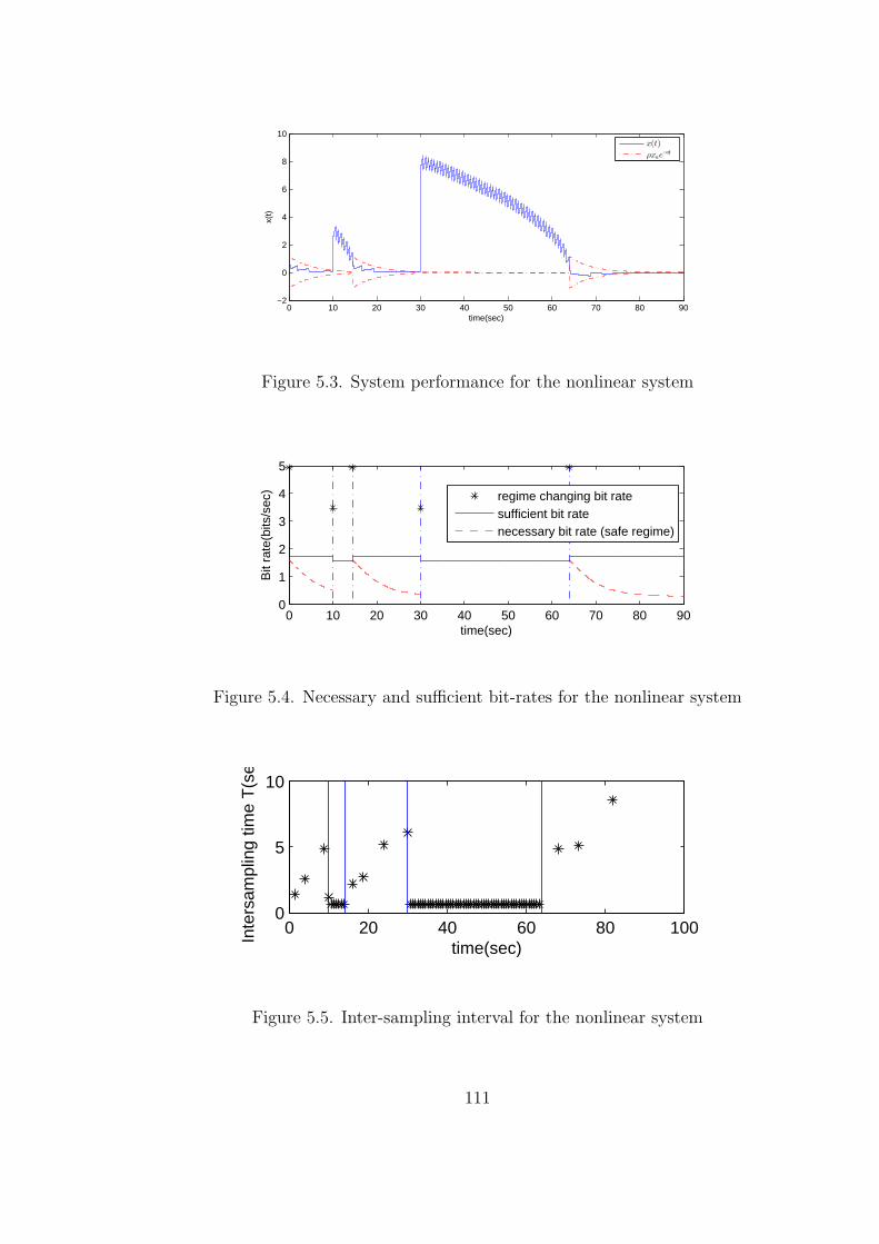
0 10 20 30 40 50 60 70 80 90−2

0

2

4

6

8

10

time(sec)

x(t)

x(t)

ρxae−αt

Figure 5.3. System performance for the nonlinear system

0 10 20 30 40 50 60 70 80 900

1

2

3

4

5

time(sec)

Bit

rate

(bits

/sec

)

regime changing bit ratesufficient bit ratenecessary bit rate (safe regime)

Figure 5.4. Necessary and sufficient bit-rates for the nonlinear system

0 20 40 60 80 1000

5

10

time(sec)

Inte

rsam

plin

g tim

e T

(sec

)

Figure 5.5. Inter-sampling interval for the nonlinear system

111

Consider the following nonlinear system:

x =

|x|sin(x) + u+ w, if |x| ≤ ρxa;

arctan(x) + u+ w, if |x| > ρxa.

with −0.9xa as the initial state. xa = 0.5 is the magnitude of absorbing region. We

choose our performance level to be β(t) = ρxae−0.2(t−t0) with ρ = 2

0.2+LL , where L = 1

is the Lipschitz constant under safe regime. L = π/2 is the uniform bound of |f(x)|

when |x| > ρxa. When the system is under unsafe regime, we choose the maximum

delay to be 1.01 of the sufficient resilience bit rate.

The system is run for 90 seconds with maximum delay, and two impulsive distur-

bances hit the system with magnitude 5xa and 15xa at time 10s and 30s, respectively.

The system performance is given in Figure 5.3 with x-axis and y-axis indicating time

and state, respectively. At time 10s and 30s, the state (solid line) jumps to 2.5 and

7.8, respectively. With the same maximum delay, which is 0.99 of the sufficient re-

silience delay, we see from the plot that the system state comes back to the absorbing

region in 5 seconds for the first attack and 34 seconds for the second attack, which

shows that as long as the bit-rate is higher than the sufficient resilience bit-rate,

no matter how far away the state is, the system is resilient, i.e. comes back to the

absorbing region in finite time. Examining the system behavior in the safe regimes

(time intervals [0, 8], [42, 50] and [58, 75]) one sees that the performance level (dot

dashed line) is guaranteed.

Figure 5.4 gives the bit-rates of the system. x-axis is time, and y-axis is bit-

rate. Since the regime changing packet has 2 bits, the corresponding bit-rate (stars)

is higher than the other packets. We also notice that there is a gap between the

necessary stabilizing bit-rates (dashed line) and the sufficient stabilizing bit-rates

(solid line) under safe regimes (intervals [0, 8], [42, 50] and [58, 75]). That is because

our sufficient stabilizing bit-rates are calculated from a global Lipschitz constant.

112

This global Lipschitz constant becomes more conservative as the state goes to 0.

The inter-sampling interval si+1 − si is given in Figure 5.5 with x-axis indicating

time and y axis indicating inter-sampling interval. In unsafe regimes, the inter-

sampling intervals are constant since we always set our delay to be the maximum

delay. In safe regimes, we can see that the inter-sampling intervals are increasing

with respect to time, or in other words, increasing as x goes to the origin, which

implies that our system is efficiently attentive [65].

To test how tight our sufficient resilience bit-rate is, we use 0.9 of the sufficient

resilience bit-rate to run the system when the system is under unsafe regime. Figure

5.6 gives the system performance with the same disturbances that we use in Figure

5.3. We can see that for the first disturbance with magnitude of 5xa, the system is

still resilient, but for the second disturbance with magnitude of 15xa, the system can’t

come back to the absorbing region again. That’s because when x = 5xa, L doesn’t

bound |f(x)| tight enough, but when x = 15xa, L is a very close upper bound on

|f(x)|.

To verify our necessary stabilizing bit-rate, we use 0.9 of this bit-rate to run the

system under safe regime. Figure 5.7 gives the system performance with initial state

to be xa. we see that the state trajectory (solid line) becomes unbounded. That’s

because the delay is so long that after the control input is applied, the state is still

above the threshold (dashed line), the event |x(t)| = θ(xa, t) will never occur, and

there is no transmission anymore. This verifies that the system can’t be stabilized

with a bit-rate lower than this necessary rate.

Now, let’s consider a linear system as below.

x =

2x+ u+ w, if |x| ≤ ρxa;

4 arctan(x) + u+ w, if |x| > ρxa,

with initial state to be 2. The magnitude of absorbing region xa is 3, and the

113

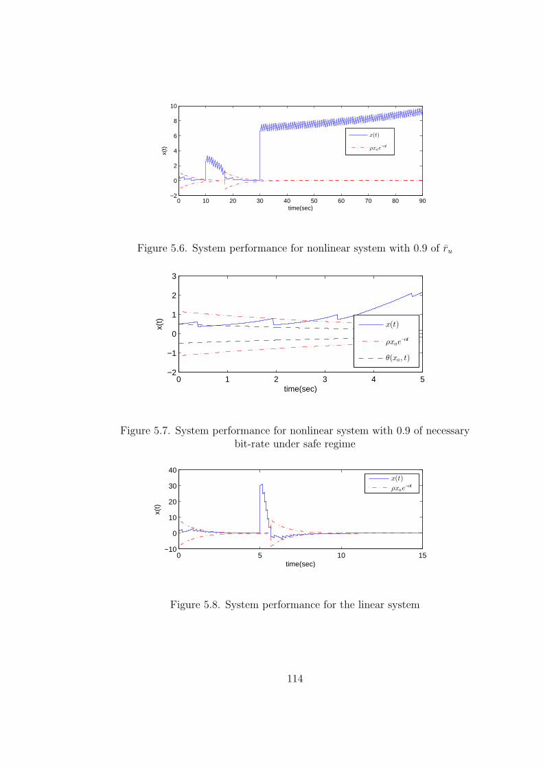
0 10 20 30 40 50 60 70 80 90−2

0

2

4

6

8

10

time(sec)

x(t)

x(t)

ρxae−αt

Figure 5.6. System performance for nonlinear system with 0.9 of ru

0 1 2 3 4 5−2

−1

0

1

2

3

time(sec)

x(t)

x(t)

ρxae−αt

θ(xa, t)

Figure 5.7. System performance for nonlinear system with 0.9 of necessarybit-rate under safe regime

0 5 10 15−10

0

10

20

30

40

time(sec)

x(t)

x(t)

ρxae−αt

Figure 5.8. System performance for the linear system

114

0 5 10 150

5

10

15

20

time(sec)B

it ra

te(b

its/s

ec)

sufficient bit ratenecessary bit rate (safe regime)

Figure 5.9. Necessary and sufficient bit-rates for the linear system

performance level is chosen to be β(t) = ρxae−α with ρ = 2

1+22 . When |x| > ρxa, the

uniform bound on |f(x)| is L = π/2. The maximum delay under unsafe regime is

chosen to be 0.12xa

L.

We ran the system for 15 seconds. Figure 5.8 shows the performance of the

system. x-axis indicates time, and y-axis indicates state. The system is attacked

at time 5s with the state (solid line) jumping to 30. We can see that the state

comes back to the absorbing region in about 2 seconds, which demonstrates that

our system is resilient. Under safe regimes, which are intervals [0, 5] and [7, 15], the

performance level (dashed line) is always guaranteed. The necessary and sufficient

bit-rates are shown in Figure 5.9 with x-axis to be the time, and y-axis indicating

bit-rate. We notice that under safe regimes, the gap between the sufficient stabilizing

bit-rate (stars) and the necessary bit-rate (dashed line) is 0 (except the first packet

indicating ’regime change’). It demonstrates our assertion that for linear systems, we

achieve the necessary stabilizing bit-rate.

5.5 Conclusions and Future Works

This chapter studies the resilience of event triggered systems against impulsive

disturbances with unknown magnitude. An even triggered strategy is provided to

achieve the resilience, and the sufficient resilience bit-rate is derived. This sufficient

115

resilience bit-rate is independent with the initial state, which means that no matter

how far away the system state is driven to, we can always use the same bit-rate to

move the state back to the absorbing region.

116

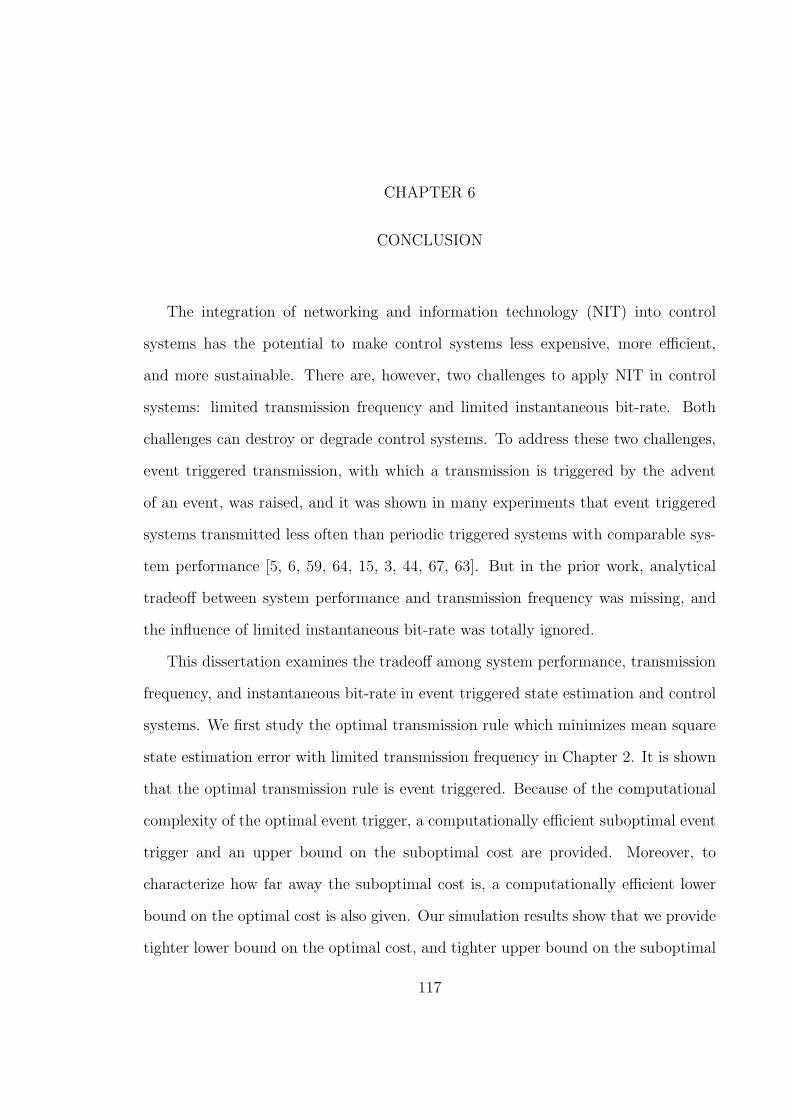
CHAPTER 6

CONCLUSION

The integration of networking and information technology (NIT) into control

systems has the potential to make control systems less expensive, more efficient,

and more sustainable. There are, however, two challenges to apply NIT in control

systems: limited transmission frequency and limited instantaneous bit-rate. Both

challenges can destroy or degrade control systems. To address these two challenges,

event triggered transmission, with which a transmission is triggered by the advent

of an event, was raised, and it was shown in many experiments that event triggered

systems transmitted less often than periodic triggered systems with comparable sys-

tem performance [5, 6, 59, 64, 15, 3, 44, 67, 63]. But in the prior work, analytical

tradeoff between system performance and transmission frequency was missing, and

the influence of limited instantaneous bit-rate was totally ignored.

This dissertation examines the tradeoff among system performance, transmission

frequency, and instantaneous bit-rate in event triggered state estimation and control

systems. We first study the optimal transmission rule which minimizes mean square

state estimation error with limited transmission frequency in Chapter 2. It is shown

that the optimal transmission rule is event triggered. Because of the computational

complexity of the optimal event trigger, a computationally efficient suboptimal event

trigger and an upper bound on the suboptimal cost are provided. Moreover, to

characterize how far away the suboptimal cost is, a computationally efficient lower

bound on the optimal cost is also given. Our simulation results show that we provide

tighter lower bound on the optimal cost, and tighter upper bound on the suboptimal

117

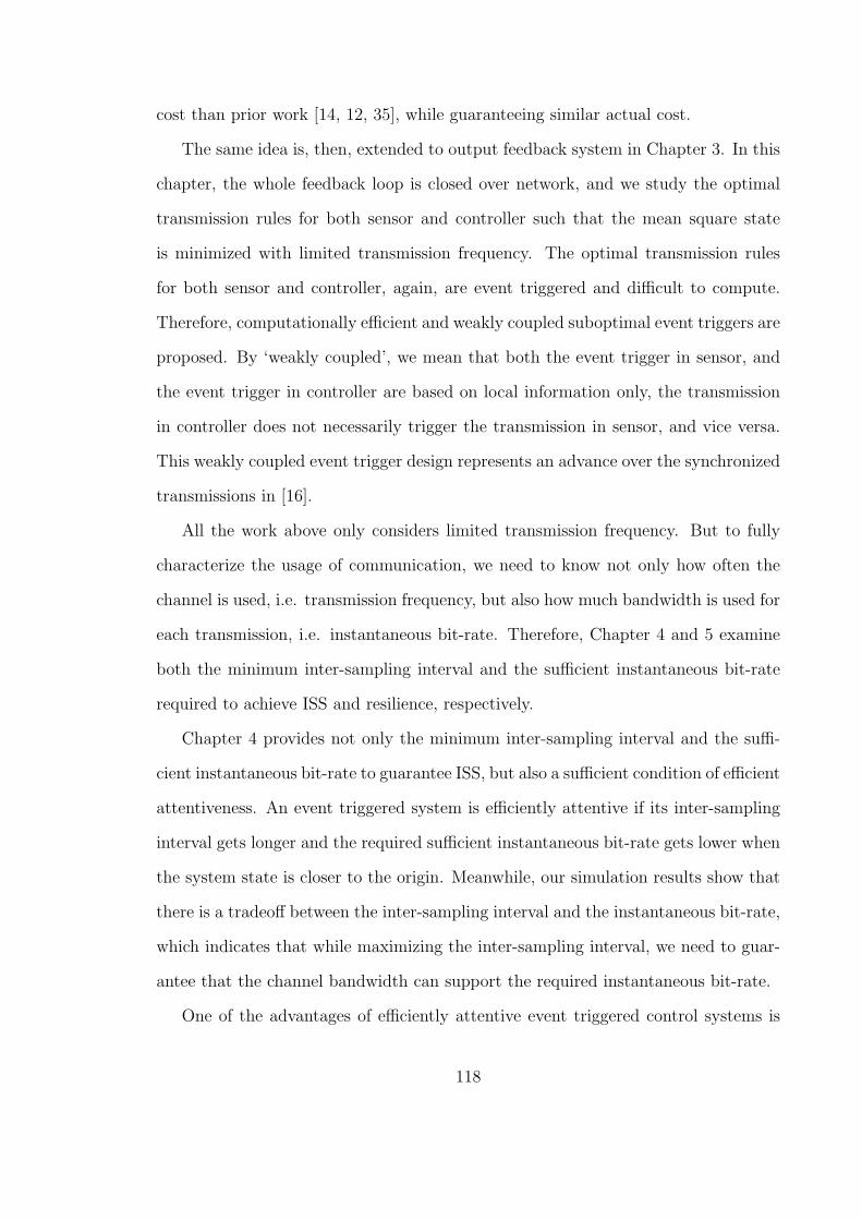
cost than prior work [14, 12, 35], while guaranteeing similar actual cost.

The same idea is, then, extended to output feedback system in Chapter 3. In this

chapter, the whole feedback loop is closed over network, and we study the optimal

transmission rules for both sensor and controller such that the mean square state

is minimized with limited transmission frequency. The optimal transmission rules

for both sensor and controller, again, are event triggered and difficult to compute.

Therefore, computationally efficient and weakly coupled suboptimal event triggers are

proposed. By ‘weakly coupled’, we mean that both the event trigger in sensor, and

the event trigger in controller are based on local information only, the transmission

in controller does not necessarily trigger the transmission in sensor, and vice versa.

This weakly coupled event trigger design represents an advance over the synchronized

transmissions in [16].

All the work above only considers limited transmission frequency. But to fully

characterize the usage of communication, we need to know not only how often the

channel is used, i.e. transmission frequency, but also how much bandwidth is used for

each transmission, i.e. instantaneous bit-rate. Therefore, Chapter 4 and 5 examine

both the minimum inter-sampling interval and the sufficient instantaneous bit-rate

required to achieve ISS and resilience, respectively.

Chapter 4 provides not only the minimum inter-sampling interval and the suffi-

cient instantaneous bit-rate to guarantee ISS, but also a sufficient condition of efficient

attentiveness. An event triggered system is efficiently attentive if its inter-sampling

interval gets longer and the required sufficient instantaneous bit-rate gets lower when

the system state is closer to the origin. Meanwhile, our simulation results show that

there is a tradeoff between the inter-sampling interval and the instantaneous bit-rate,

which indicates that while maximizing the inter-sampling interval, we need to guar-

antee that the channel bandwidth can support the required instantaneous bit-rate.

One of the advantages of efficiently attentive event triggered control systems is

118

that long inter-sampling interval can be achieved when the system state is close to

its equilibrium. A concern about this long inter-sampling interval is whether event

triggered system is resilient to unexpected disturbances between two consecutive

transmissions. Chapter 5 addresses this concern by considering a train of transient

unknown magnitude disturbances in a scalar nonlinear system. The system is ana-

lyzed under two operational regimes: safe and unsafe. Under safe regime, a necessary

instantaneous bit-rate and a sufficient instantaneous bit-rate are presented to guar-

antee uniform boundedness, and the necessary bit-rate meets the sufficient bit-rate

when the system is linear. Under unsafe regime, a sufficient instantaneous bit-rate

is given to guarantee resilience, i.e. returning to a neighborhood of the origin in a

finite time. Moreover, detailed algorithms under both safe and unsafe regime are

provided, and our simulation results demonstrate that event triggered systems are

indeed resilient to transient unknown magnitude disturbances.

119

APPENDIX A

Proofs

Lemma A.0.1. The filtered state error, eKF (k) is orthogonal to eKF,RO(k).

Proof. Since Kalman filter is the minimum mean square estimate of the state based on

all history measurements y(0), . . . , y(k), the estimation error eKF (k) is orthogonal

to any function of the history measurements y(0), . . . , y(k). Since both xKF (k)

and xRO(k) (see equation (2.11) and (2.12)) are functions of history measurements

y(0), . . . , y(k), eKF (k) is orthogonal to eKF,RO(k).

Lemma A.0.2. Let l(k) = maxl : τ ls ≤ k

indicate the latest transmission time

from the sensor subsystem to the controller subsystem. The a posteriori history in-

formation H(k) is

H(k) =τ 1s , τ

2s , · · · , τ l(k)s , xKF (τ

1s ), xKF (τ

2s ), · · · , xKF (τ

l(k)s ),

ua(0), ua(1), . . . , ua(k − 1) ,

for k = 0, 1, . . .. Correspondingly, we also define the a priori history information,

the history information known by the controller subsystem before the event detector

in sensor subsystem decides whether to transmit at step k, H−(k) as

H−(k) =τ 1s , τ

2s , · · · , τ l(k−1)

s , xKF (τ1s ), xKF (τ

2s ), · · · , xKF (τ

l(k−1)s ),

ua(0), ua(1), . . . , ua(k − 1) .

120

for k = 0, 1, . . . with H−(0) = ∅. The a posteriori remote state estimate in equation

(3.2) satisfies

xRO(k) = E(x(k)|H(k)),

and the a priori remote state estimate x−RO(k) in equation (3.1) satisfies

x−RO(k) = E(x(k)|H−(k)).

Proof. Now, let’s examine how the remote state estimate evolves. The initial condi-

tion is

x−RO(0) = E(x(k)|H−(0)) = µ0.

If information is transmitted from sensor to controller at step k, the history in-

formation at step k is H(k) = H−(k), xKF (k), and the a posteriori remote state

estimate is

xRO(k) = E(x(k)|H−(k), xKF (k))

= E(xKF (k) + eKF (k)|H−(k), xKF (k))

= xKF (k),

where the second equality holds because eKF (k) is uncorrelated with H(k).

If information is not transmitted from sensor to controller at step k, the history

information at step k is H(k) = H−(k), and the a posteriori remote state estimate is

121

the same as the a priori remote state estimate, i.e.

xRO(k) = E(x(k)|H(k)) = E(x(k)|H−(k))

= x−RO(k).

The a priori state estimate evolves as the following:

x−RO(k) = E(x(k)|H−(k))

= E(Ax(k − 1) +Bua(k − 1) + w(k − 1)|H−(k))

= AE(x(k − 1)|H−(k)) +Bua(k − 1)

= AxRO(k − 1) +Bua(k − 1),

where the third equality holds because w(k − 1) is independent from H−(k).

To conclude, we say that the minimum mean square remote state estimate based

on H(k) takes the form of equation (3.1) and (3.2).

122

BIBLIOGRAPHY

1. H. Alemdar and C. Ersoy. Wireless sensor networks for healthcare: A survey.Computer Networks, 54(15):2688–2710, 2010.

2. G. Anastasi, M. Conti, M. Di Francesco, and A. Passarella. Energy conservationin wireless sensor networks: A survey. Ad Hoc Networks, 7(3):537–568, 2009.

3. A. Anta and P. Tabuada. To sample or not to sample: Self-triggered controlfor nonlinear systems. In Automatic Control, IEEE Transactions on, volume 55,pages 2030–2042. IEEE, 2010.

4. A. Arapostathis, V. Borkar, E. Fernandez-Gaucherand, M. Ghosh, and S. Marcus.Discrete-time controlled markov processes with average cost criterion: a survey.SIAM Journal on Control and Optimization, 31(2):282–344, 1993.

5. K. Arzen. A simple event-based pid controller. In Proc. 14th IFAC WorldCongress, volume 18, pages 423–428, 1999.

6. K. Astrom and B. Bernhardsson. Comparison of Riemann and Lebesgue samplingfor first order stochastic systems. In Decision and Control, 2002, Proceedings ofthe 41st IEEE Conference on, volume 2, pages 2011–2016. IEEE, 2002. ISBN0780375165.

7. S. Bayraktar. Aggressive landing maneuvers for unmanned aerial vehicles. PhDthesis, Massachusetts Institute of Technology, 2006.

8. S. Boyd and L. Vandenberghe. Convex optimization. Cambridge university press,2004.

9. R. Brockett and D. Liberzon. Quantized feedback stabilization of linear systems.Automatic Control, IEEE Transactions on, 45(7):1279–1289, 2000.

10. M. Cardei and D.-Z. Du. Improving wireless sensor network lifetime throughpower aware organization. Wireless Networks, 11(3):333–340, 2005.

11. M. Choi, T. Lam, and B. Reznick. Sums of squares of real polynomials. In Pro-ceedings of Symposia in Pure Mathematics, volume 58, pages 103–126. AmericanMathematical Society, 1995.

123

12. R. Cogill. Event-based control using quadratic approximate value functions.In Decision and Control, 2009 held jointly with the 2009 28th Chinese ControlConference. CDC/CCC 2009. Proceedings of the 48th IEEE Conference on, pages5883–5888. IEEE, 2009.

13. R. Cogill and S. Lall. Suboptimality bounds in stochastic control: A queueingexample. In American Control Conference, 2006, pages 1642–1647. IEEE, 2006.

14. R. Cogill, S. Lall, and J. Hespanha. A constant factor approximation algorithmfor event-based sampling. In American Control Conference, 2007. ACC’07, pages305–311. IEEE, 2007.

15. D. V. Dimarogonas and K. H. Johansson. Event-triggered control for multi-agentsystems. In Decision and Control, 2009 held jointly with the 2009 28th ChineseControl Conference. CDC/CCC 2009. Proceedings of the 48th IEEE Conferenceon, pages 7131–7136. IEEE, 2009.

16. M. Donkers and W. Heemels. Output-based event-triggered control with guar-anteed L8-gain and improved event-triggering. In Proceedings of the 49th IEEEConference on Decision and Control, 2010.

17. E. Dynkin and A. Juskevic. Controlled markov processes, volume 235. SpringerNew York, 1979.

18. H. Farhangi. The path of the smart grid. Power and Energy Magazine, IEEE, 8(1):18–28, 2010.

19. D. Finkel. Direct optimization algorithm user guide. Center for Research inScientific Computation, North Carolina State University, 2, 2003.

20. E. Garcia and P. J. Antsaklis. Model-based event-triggered control with time-varying network delays. In Decision and Control and European Control Con-ference (CDC-ECC), 2011 50th IEEE Conference on, pages 1650–1655. IEEE,2011.

21. E. Gordienko and O. Hernandez-Lerma. Average cost markov control processeswith weighted norms: value iteration. Appl. Math, 23:219–237, 1995.

22. X. Guo and Q. Zhu. Average optimality for markov decision processes in borelspaces: a new condition and approach. Journal of Applied Probability, 43(2):318–334, 2006.

23. R. A. Gupta and M.-Y. Chow. Networked control system: Overview and researchtrends. Industrial Electronics, IEEE Transactions on, 57(7):2527–2535, 2010.

24. W. Heemels, J. Sandee, and P. Van Den Bosch. Analysis of event-driven con-trollers for linear systems. In International Journal of Control, volume 81, pages571–590. Taylor & Francis, 2008.

124

25. O. Hernandez-Lerma and J. Lasserre. Discrete-time Markov control processes:basic optimality criteria. Springer New York, 1996.

26. O. Hernandez-Lerma and J. Lasserre. Policy iteration for average cost markovcontrol processes on borel spaces. Acta Applicandae Mathematicae, 47(2):125–154, 1997.

27. J. Hespanha, A. Ortega, and L. Vasudevan. Towards the control of linear systemswith minimum bit-rate. 2002.

28. Y.-F. Huang, S. Werner, J. Huang, N. Kashyap, and V. Gupta. State estimationin electric power grids: Meeting new challenges presented by the requirements ofthe future grid. Signal Processing Magazine, IEEE, 29(5):33–43, 2012.

29. O. Imer and T. Basar. Optimal estimation with limited measurements. In De-cision and Control, 2005 and 2005 European Control Conference. CDC-ECC’05.44th IEEE Conference on, pages 1029–1034. IEEE, 2005. ISBN 0780395670.

30. O. Imer and T. Basar. Optimal estimation with scheduled measurements. InAppl. Comput. Math, volume 4, pages 92–101, 2005.

31. L. Isserlis. On a formula for the product-moment coefficient of any order of anormal frequency distribution in any number of variables. Biometrika, 12(1/2):134–139, 1918.

32. H. Khalil and J. Grizzle. Nonlinear systems, volume 3. Prentice hall, 1992.

33. D. Lehmann and J. Lunze. Event-based control with communication delays.In Proceedings of the 18th International Federation of Automatic ControlWorldCongress (IFAC’11), pages 3262–3267, 2011.

34. L. Li and M. Lemmon. Event-Triggered Output Feedback Control of FiniteHorizon Discrete-time Multi-dimensional Linear Processes. In Proceedings of the49th IEEE Conference on Decision and Control, 2010.

35. L. Li and M. Lemmon. Performance and average sampling period of sub-optimaltriggering event in event triggered state estimation. In Conference of decisionand control. IEEE, 2011.

36. L. Li and M. Lemmon. Weakly coupled event triggered output feedback controlin wireless networked control systems. In Communication, Control, and Comput-ing (Allerton), 2011 49th Annual Allerton Conference on, pages 572–579. IEEE,2011.

37. L. Li and M. Lemmon. Computationally efficient suboptimal event trigger designfor MMSE problem with limited communication. submitted to IEEE Transactionof Automatic Control, 2013.

125

38. L. Li and M. Lemmon. Efficient attentive event triggered control systems withlimited bandwidth. submitted to IEEE Transaction of Automatic Control, 2013.

39. L. Li and M. Lemmon. Polynomial Approximation of Optimal Event Triggers forState Estimation Problems Using SOSTOOLS. In American Control Conference(ACC), 2013, 2013.

40. L. Li, M. Lemmon, and X. Wang. Event-triggered state estimation in vectorlinear processes. In American Control Conference (ACC), 2010, pages 2138–2143. IEEE, 2010.

41. L. Li, M. Lemmon, and X. Wang. Stabilizing bit-rates in quantized event trig-gered control systems. In Hybrid Systems: Computation and Control, 2012.

42. L. L. Li and M. Lemmon. Weakly coupled event triggered output feedback systemin wireless networked control systems. to appear in Discrete Event DynamicSystem, 2013. URL http://www3.nd.edu/~lli3/publications/deds.pdf.

43. L. L. Li, X. Wang, and M. Lemmon. Stabilizing bit-rates in disturbed eventtriggered control systems. In the 4th IFAC Conference on Analysis and Designof Hybrid Systems, 2012.

44. J. Lunze and D. Lehmann. A state-feedback approach to event-based control. InAutomatica, volume 46, pages 211–215. Elsevier, 2010.

45. M. Mazo and P. Tabuada. On event-triggered and self-triggered control oversensor/actuator networks. In Decision and Control, 2008. CDC 2008. 47th IEEEConference on, pages 435–440. IEEE, 2008.

46. M. Mazo and P. Tabuada. Decentralized event-triggered control over wirelesssensor/actuator networks. Automatic Control, IEEE Transactions on, 56(10):2456–2461, 2011.

47. S. Meyn. The policy iteration algorithm for average reward markov decisionprocesses with general state space. Automatic Control, IEEE Transactions on,42(12):1663–1680, 1997.

48. A. Molin and S. Hirche. Structural characterization of optimal event-based con-trollers for linear stochastic systems. In Proceedings of the 49th IEEE Conferenceon Decision and Control, 2010.

49. P. Parrilo. Semidefinite programming relaxations for semialgebraic problems.Mathematical Programming, 96(2):293–320, 2003.

50. G. J. Pottie and W. J. Kaiser. Wireless integrated network sensors. Communi-cations of the ACM, 43(5):51–58, 2000.

51. V. Powers and T. Wormann. An algorithm for sums of squares of real polyno-mials. Journal of pure and applied algebra, 127(1):99–104, 1998.

126

52. S. Prajna, A. Papachristodoulou, P. Seiler, and P. Parrilo. Sostools: Sum ofsquares optimization toolbox for matlab. Users guide, 2004.

53. M. L. Puterman. Markov decision processes: discrete stochastic dynamic pro-gramming, volume 414. Wiley-Interscience, 2009.

54. M. Rabi, G. Moustakides, and J. Baras. Multiple sampling for estimation on afinite horizon. In Decision and Control, 2006 45th IEEE Conference on, pages1351–1357. IEEE, 2006. ISBN 1424401712.

55. V. Raghunathan, C. Schurgers, S. Park, and M. B. Srivastava. Energy-awarewireless microsensor networks. Signal Processing Magazine, IEEE, 19(2):40–50,2002.

56. C. Rieger, D. Gertman, and M. McQueen. Resilient control systems: next gen-eration design research. In Human System Interactions, 2009. HSI’09. 2nd Con-ference on, pages 632–636. IEEE, 2009.

57. P. Santi. Topology control in wireless ad hoc and sensor networks. ACM Com-puting Surveys (CSUR), 37(2):164–194, 2005.

58. S. M. L. C. (SMLC). Implementing 21st century smart nanufacturing. WorkshopSummary Report. URL https://smart-process-manufacturing.ucla.edu/

about/news/Smart%20Manufacturing%206_24_11.pdf.

59. P. Tabuada. Event-triggered real-time scheduling of stabilizing control tasks.Automatic Control, IEEE Transactions on, 52(9):1680–1685, 2007. ISSN 0018-9286.

60. S. Tatikonda and S. Mitter. Control under communication constraints. AutomaticControl, IEEE Transactions on, 49(7):1056–1068, 2004.

61. M. H. ten Berge, B. Orlic, and J. F. Broenink. Co-simulation of networkedembedded control systems, a csp-like process-oriented approach. In ComputerAided Control System Design, 2006 IEEE International Conference on ControlApplications, 2006 IEEE International Symposium on Intelligent Control, 2006IEEE, pages 434–439. IEEE, 2006.

62. K. Toh, M. Todd, and R. Tutuncu. Sdpt3 - a matlab software package forsemidefinite programming. Optimization Methods and Software, 11(1-4):545–581,1999.

63. P. Wan and M. D. Lemmon. Event-triggered distributed optimization in sensornetworks. In Information Processing in Sensor Networks, 2009. IPSN 2009.International Conference on, pages 49–60. IEEE, 2009.

64. X. Wang and M. Lemmon. Self-Triggered Feedback Control Systems With Finite-Gain L2 Stability. In Automatic Control, IEEE Transactions on, volume 54,pages 452–467. IEEE, 2009.

127

65. X. Wang and M. Lemmon. Attentively efficient controllers for event-triggeredfeedback systems. In IEEE Conference on Decsion and Control, 2011.

66. X. Wang and M. Lemmon. Minimum attention controllers for event-triggeredfeedback systems. In IEEE Conference on Decision and Control-European Con-trol Conference, 2011.

67. X. Wang and M. D. Lemmon. Event-triggering in distributed networked controlsystems. Automatic Control, IEEE Transactions on, 56(3):586–601, 2011.

68. T. Wark, P. Corke, P. Sikka, L. Klingbeil, Y. Guo, C. Crossman, P. Valencia,D. Swain, and G. Bishop-Hurley. Transforming agriculture through pervasivewireless sensor networks. Pervasive Computing, IEEE, 6(2):50–57, 2007.

69. W. Wong and R. Brockett. Systems with finite communication bandwidth con-straints. ii. stabilization with limited information feedback. Automatic Control,IEEE Transactions on, 44(5):1049–1053, 1999.

70. Y. Xu and J. Hespanha. Optimal communication logics in networked control sys-tems. In Proceedings of the IEEE Conference on Decision and Control, volume 4,pages 3527–3532, Nassau, Bahamas, 2004.

71. H. Yu and P. J. Antsaklis. Event-triggered output feedback control for networkedcontrol systems using passivity: Triggering condition and limitations. In Decisionand Control and European Control Conference (CDC-ECC), 2011 50th IEEEConference on, pages 199–204. IEEE, 2011.

72. D. Yue, E. Tian, and Q.-L. Han. A delay system method to design of event-triggered control of networked control systems. In Decision and Control and Eu-ropean Control Conference (CDC-ECC), 2011 50th IEEE Conference on, pages1668–1673. IEEE, 2011.

73. Q. Zhu and T. Basar. Robust and resilient control design for cyber-physicalsystems with an application to power systems. In Proc. of 50th IEEE Conferenceon Decision and Control and European Control Conference, Orlando, Florida,2011.

This document was prepared & typeset with LATEX2ε, and formatted withnddiss2ε classfile (v3.2013[2013/04/16]) provided by Sameer Vijay and updated

by Megan Patnott.

128

This Dissertation 2 - University of Notre DameThis Dissertation entitled EVENT TRIGGERED STATE...

Documents

Transcript of This Dissertation 2 - University of Notre DameThis Dissertation entitled EVENT TRIGGERED STATE...