The Wave Equation in 1D and 2D

Knut–Andreas Lie

Dept. of Informatics, University of Oslo

INF2340 / Spring 2005 – p. 1

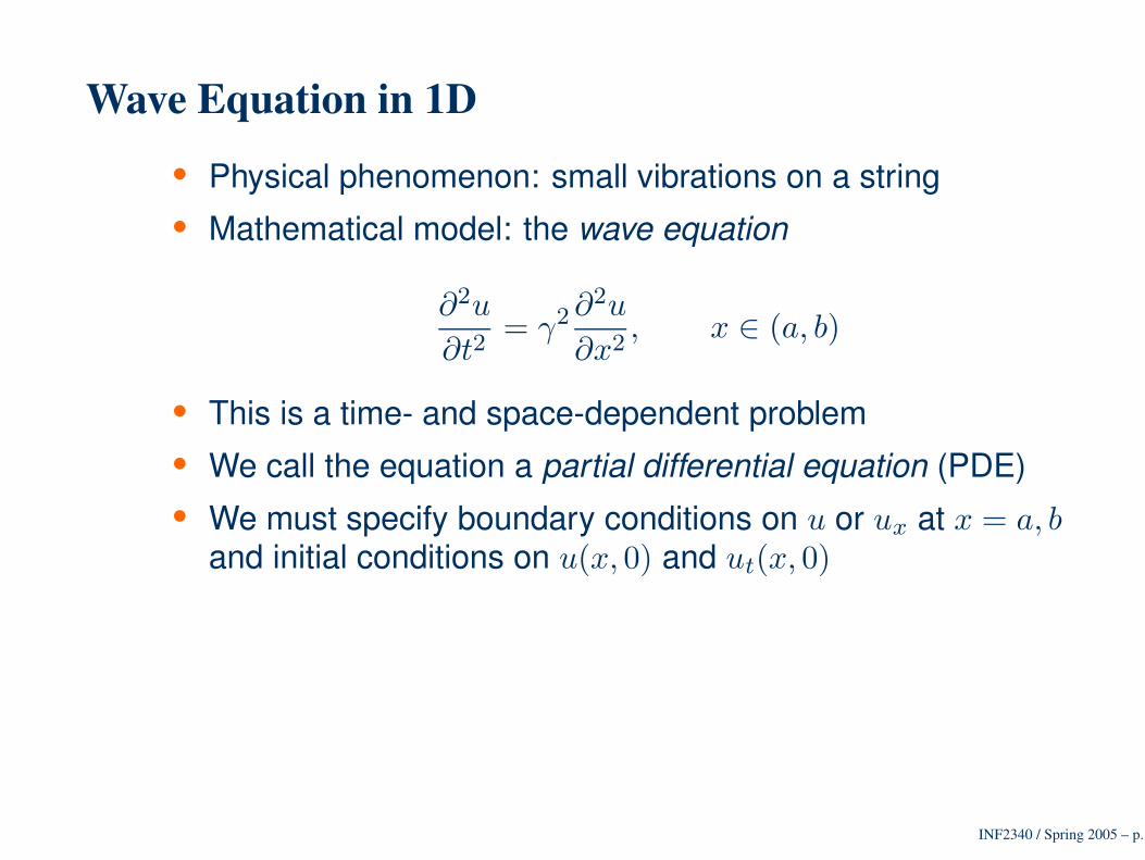
Wave Equation in 1D• Physical phenomenon: small vibrations on a string• Mathematical model: the wave equation

∂2u

∂t2= γ2 ∂2u

∂x2, x ∈ (a, b)

• This is a time- and space-dependent problem• We call the equation a partial differential equation (PDE)• We must specify boundary conditions on u or ux at x = a, b

and initial conditions on u(x, 0) and ut(x, 0)

INF2340 / Spring 2005 – p. 2

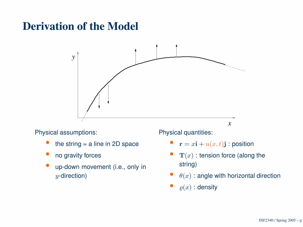
Derivation of the Model

y

xPhysical assumptions:

• the string = a line in 2D space

• no gravity forces

• up-down movement (i.e., only iny-direction)

Physical quantities:

• r = xi + u(x, t)j : position

• T(x) : tension force (along thestring)

• θ(x) : angle with horizontal direction

• %(x) : density

INF2340 / Spring 2005 – p. 3

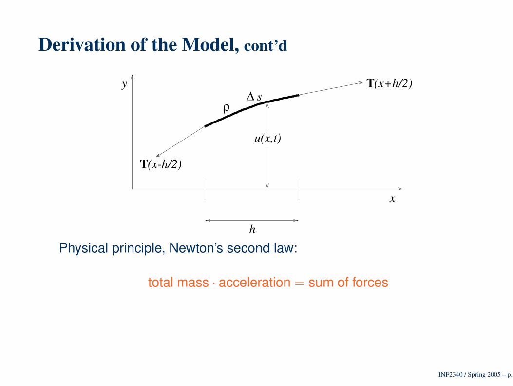
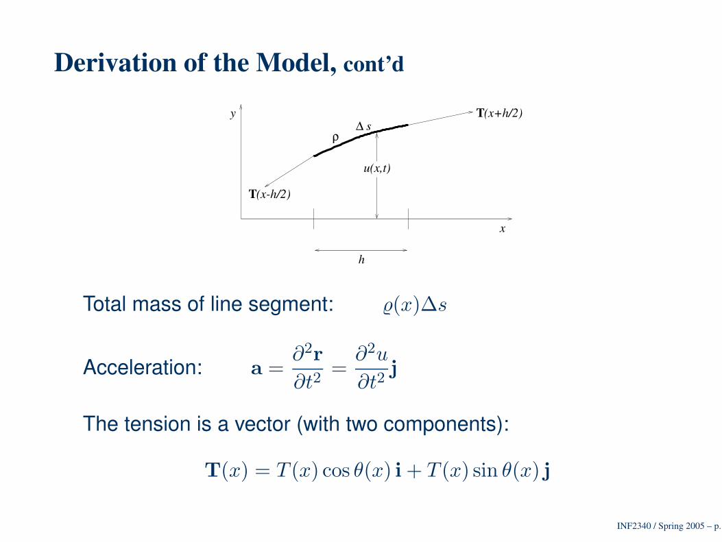
Derivation of the Model, cont’d

y

x

T

T

(x-h/2)

(x+h/2)

u(x,t)

ρ∆ s

h

Physical principle, Newton’s second law:

total mass · acceleration = sum of forces

INF2340 / Spring 2005 – p. 4

Derivation of the Model, cont’d

y

x

T

T

(x-h/2)

(x+h/2)

u(x,t)

ρ∆ s

h

Total mass of line segment: %(x)∆s

Acceleration: a =∂2r

∂t2=

∂2u

∂t2j

The tension is a vector (with two components):

T(x) = T (x) cos θ(x) i + T (x) sin θ(x) j

INF2340 / Spring 2005 – p. 5

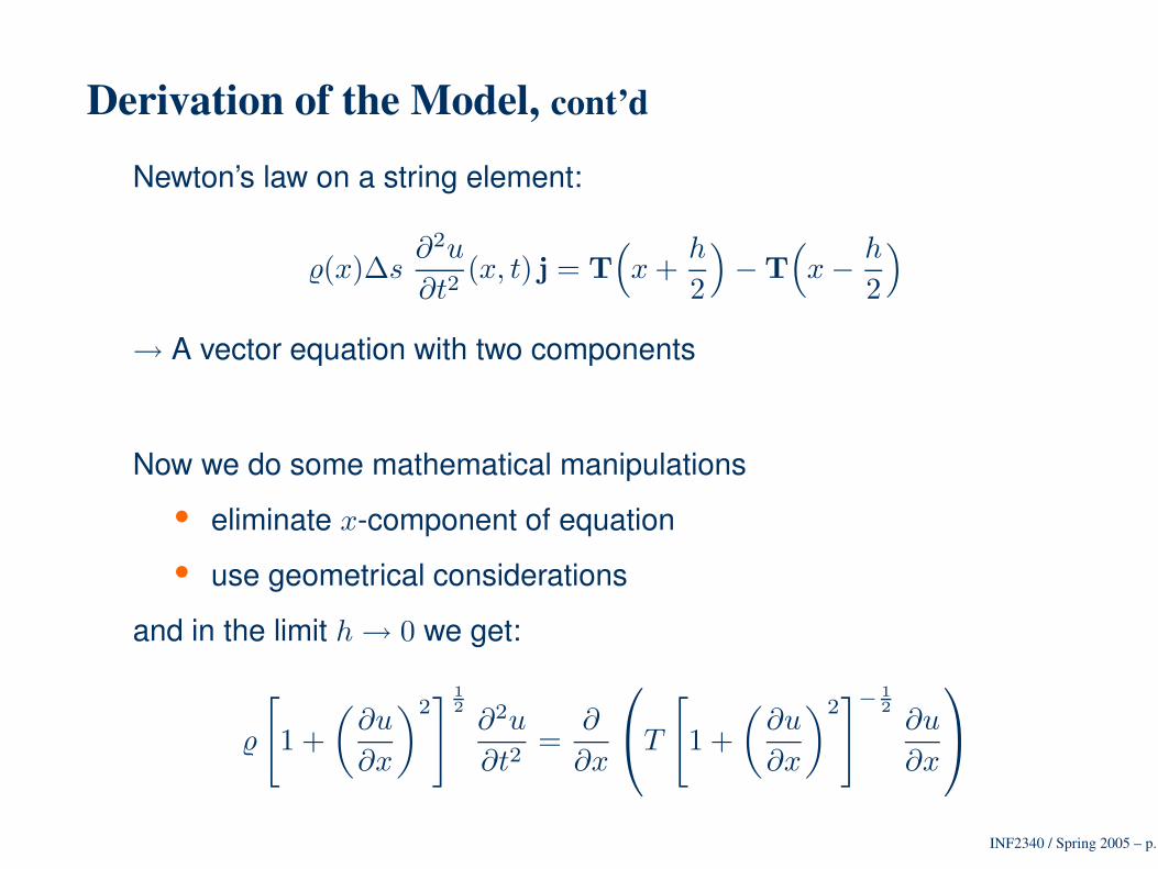
Derivation of the Model, cont’d

Newton’s law on a string element:

%(x)∆s∂2u

∂t2(x, t) j = T

(

x +h

2

)

−T(

x−h

2

)

→ A vector equation with two components

Now we do some mathematical manipulations

• eliminate x-component of equation

• use geometrical considerations

and in the limit h→ 0 we get:

%

[

1 +

(

∂u

∂x

)2]

12

∂2u

∂t2=

∂

∂x

T

[

1 +

(

∂u

∂x

)2]

−

12

∂u

∂x

INF2340 / Spring 2005 – p. 6

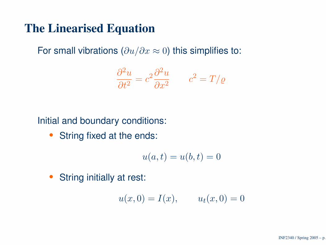
The Linearised Equation

For small vibrations (∂u/∂x ≈ 0) this simplifies to:

∂2u

∂t2= c2 ∂2u

∂x2c2 = T/%

Initial and boundary conditions:• String fixed at the ends:

u(a, t) = u(b, t) = 0

• String initially at rest:

u(x, 0) = I(x), ut(x, 0) = 0

INF2340 / Spring 2005 – p. 7

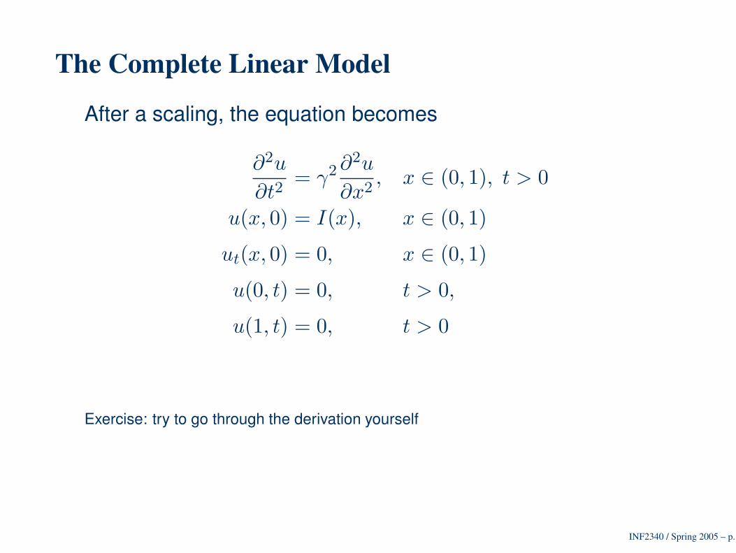
The Complete Linear Model

After a scaling, the equation becomes

∂2u

∂t2= γ2 ∂2u

∂x2, x ∈ (0, 1), t > 0

u(x, 0) = I(x), x ∈ (0, 1)

ut(x, 0) = 0, x ∈ (0, 1)

u(0, t) = 0, t > 0,

u(1, t) = 0, t > 0

Exercise: try to go through the derivation yourself

INF2340 / Spring 2005 – p. 8

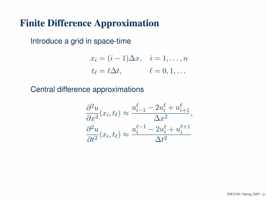
Finite Difference Approximation

Introduce a grid in space-time

xi = (i− 1)∆x, i = 1, . . . , n

t` = `∆t, ` = 0, 1, . . .

Central difference approximations

∂2u

∂x2(xi, t`) ≈

u`i−1 − 2u`

i + u`i+1

∆x2,

∂2u

∂t2(xi, t`) ≈

u`−1i − 2u`

i + u`+1i

∆t2

INF2340 / Spring 2005 – p. 9

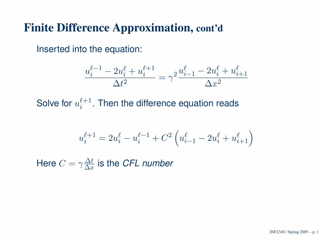
Finite Difference Approximation, cont’d

Inserted into the equation:

u`−1i − 2u`

i + u`+1i

∆t2= γ2 u`

i−1 − 2u`i + u`

i+1

∆x2

Solve for u`+1i . Then the difference equation reads

u`+1i = 2u`

i − u`−1i + C2

(

u`i−1 − 2u`

i + u`i+1

)

Here C = γ ∆t∆x is the CFL number

INF2340 / Spring 2005 – p. 10

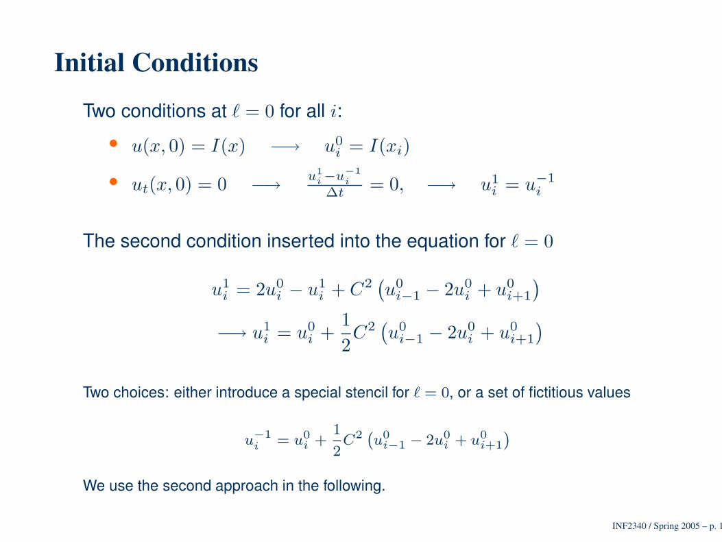
Initial Conditions

Two conditions at ` = 0 for all i:

• u(x, 0) = I(x) −→ u0i = I(xi)

• ut(x, 0) = 0 −→u1

i−u−1

i

∆t = 0, −→ u1i = u−1

i

The second condition inserted into the equation for ` = 0

u1i = 2u0

i − u1i + C2

(

u0i−1 − 2u0

i + u0i+1

)

−→ u1i = u0

i +1

2C2(

u0i−1 − 2u0

i + u0i+1

)

Two choices: either introduce a special stencil for ` = 0, or a set of fictitious values

u−1

i = u0i +

1

2C2

`

u0i−1 − 2u0

i + u0i+1

´

We use the second approach in the following.

INF2340 / Spring 2005 – p. 11

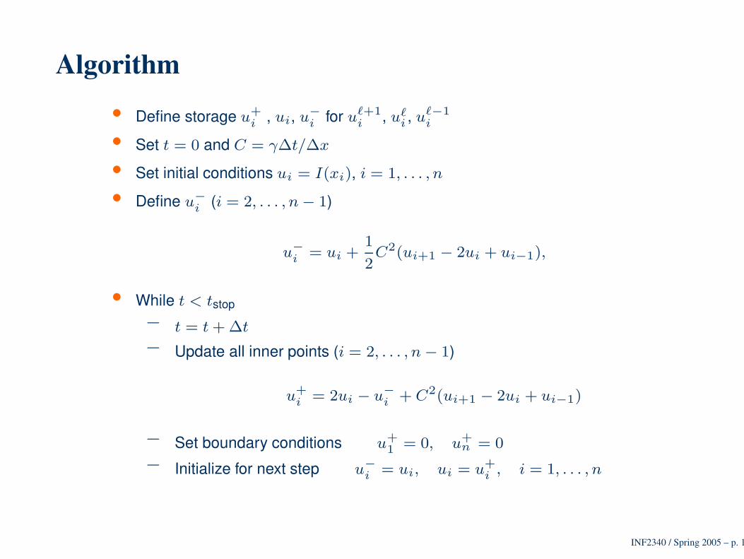
Algorithm• Define storage u+

i , ui, u−

i for u`+1

i , u`i , u`−1

i

• Set t = 0 and C = γ∆t/∆x

• Set initial conditions ui = I(xi), i = 1, . . . , n

• Define u−

i (i = 2, . . . , n − 1)

u−

i = ui +1

2C2(ui+1 − 2ui + ui−1),

• While t < tstop

− t = t + ∆t

− Update all inner points (i = 2, . . . , n − 1)

u+

i = 2ui − u−

i + C2(ui+1 − 2ui + ui−1)

− Set boundary conditions u+

1= 0, u+

n = 0

− Initialize for next step u−

i = ui, ui = u+

i , i = 1, . . . , n

INF2340 / Spring 2005 – p. 12

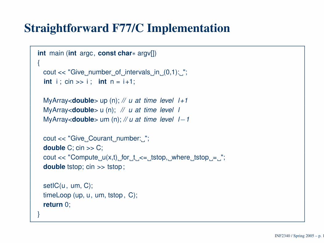
Straightforward F77/C Implementation

int main (int argc, const char∗ argv[])

cout << "Give number of intervals in (0,1): ";int i ; cin >> i ; int n = i+1;

MyArray<double> up (n); // u at time level l+1MyArray<double> u (n); // u at time level lMyArray<double> um (n); // u at time level l−1

cout << "Give Courant number: ";double C; cin >> C;cout << "Compute u(x,t) for t <= tstop, where tstop = ";double tstop; cin >> tstop ;

setIC(u , um, C);timeLoop (up, u, um, tstop , C);return 0;

INF2340 / Spring 2005 – p. 13

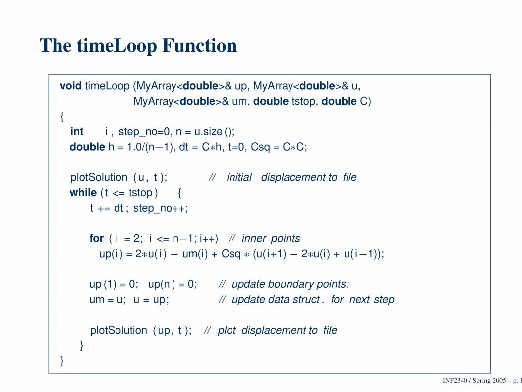
The timeLoop Function

void timeLoop (MyArray<double>& up, MyArray<double>& u,MyArray<double>& um, double tstop, double C)

int i , step_no=0, n = u.size ();double h = 1.0/(n−1), dt = C∗h, t=0, Csq = C∗C;

plotSolution ( u , t ); // initial displacement to filewhile ( t <= tstop )

t += dt ; step_no++;

for ( i = 2; i <= n−1; i++) // inner pointsup(i ) = 2∗u( i ) − um(i) + Csq ∗ (u( i+1) − 2∗u(i ) + u( i−1));

up (1) = 0; up(n ) = 0; // update boundary points:um = u; u = up; // update data struct . for next step

plotSolution ( up, t ); // plot displacement to file

INF2340 / Spring 2005 – p. 14

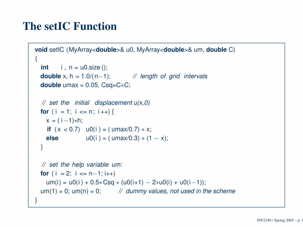
The setIC Function

void setIC (MyArray<double>& u0, MyArray<double>& um, double C)

int i , n = u0.size ();double x, h = 1.0/(n−1); // length of grid intervalsdouble umax = 0.05, Csq=C∗C;

// set the initial displacement u(x,0)for ( i = 1; i <= n; i ++)

x = ( i−1)∗h;if ( x < 0.7) u0(i ) = ( umax/0.7) ∗ x;else u0(i ) = ( umax/0.3) ∗ (1 − x);

// set the help variable um:for ( i = 2; i <= n−1; i++)

um(i) = u0(i ) + 0.5∗Csq ∗ (u0(i+1) − 2∗u0(i) + u0(i−1));um(1) = 0; um(n) = 0; // dummy values, not used in the scheme

INF2340 / Spring 2005 – p. 15

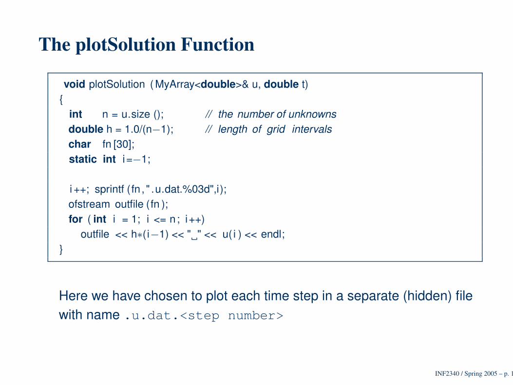
The plotSolution Function

void plotSolution ( MyArray<double>& u, double t)

int n = u.size (); // the number of unknownsdouble h = 1.0/(n−1); // length of grid intervalschar fn [30];static int i=−1;

i ++; sprintf (fn , " .u.dat.%03d",i);ofstream outfile (fn );for ( int i = 1; i <= n; i++)

outfile << h∗(i−1) << " " << u( i ) << endl;

Here we have chosen to plot each time step in a separate (hidden) filewith name .u.dat.<step number>

INF2340 / Spring 2005 – p. 16

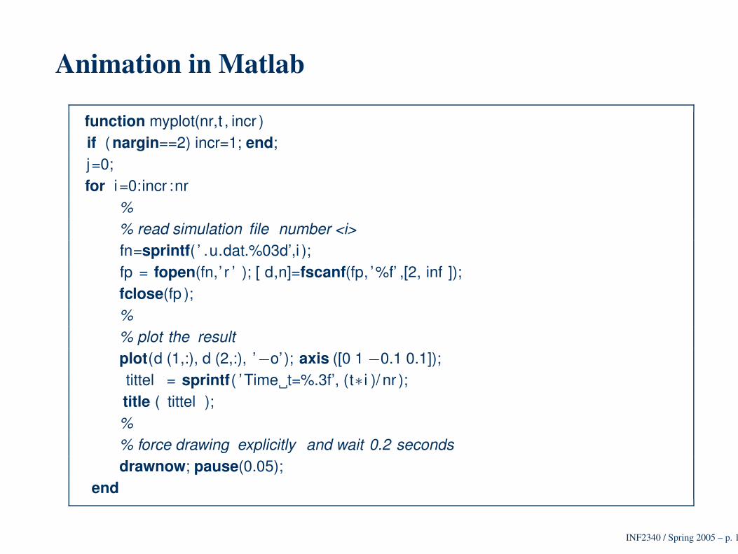
Animation in Matlab

function myplot(nr,t , incr )if ( nargin==2) incr=1; end;j=0;for i=0:incr :nr

%% read simulation file number <i>fn=sprintf( ’ .u.dat.%03d’,i );fp = fopen(fn,’ r ’ ); [ d,n]=fscanf(fp, ’%f’ ,[2, inf ]);fclose(fp );%% plot the resultplot(d (1,:), d (2,:), ’−o’); axis ([0 1 −0.1 0.1]);tittel = sprintf( ’Time t=%.3f’, (t∗ i )/ nr );title ( tittel );%% force drawing explicitly and wait 0.2 secondsdrawnow; pause(0.05);

end

INF2340 / Spring 2005 – p. 17

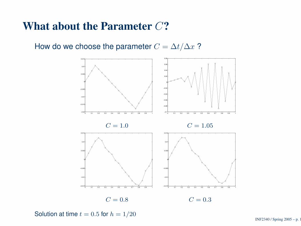
What about the Parameter C?

How do we choose the parameter C = ∆t/∆x ?

0 0.1 0.2 0.3 0.4 0.5 0.6 0.7 0.8 0.9 1−0.02

−0.015

−0.01

−0.005

0

0.005

0.01

0.015

0 0.1 0.2 0.3 0.4 0.5 0.6 0.7 0.8 0.9 1−0.1

−0.08

−0.06

−0.04

−0.02

0

0.02

0.04

0.06

0.08

C = 1.0 C = 1.05

0 0.1 0.2 0.3 0.4 0.5 0.6 0.7 0.8 0.9 1−0.015

−0.01

−0.005

0

0.005

0.01

0.015

0 0.1 0.2 0.3 0.4 0.5 0.6 0.7 0.8 0.9 1−0.015

−0.01

−0.005

0

0.005

0.01

0.015

C = 0.8 C = 0.3

Solution at time t = 0.5 for h = 1/20INF2340 / Spring 2005 – p. 18

Numerical Stability and Accuracy• We have two parameters, ∆t and ∆x, that are related through

C = ∆t/∆x

• How do we choose ∆t and ∆x?

• Too large values of ∆t and ∆x give

- too large numerical errors

- or in the worst case: unstable solutions

• Too small ∆t and ∆x means too much computing power

• Simplified problems can be analysed theoretically

⇒ Guide to choosing ∆t and ∆x

INF2340 / Spring 2005 – p. 19

Large Destructive Water Waves

The wave equations may also be used to simulate largedestructive waves• Waves in fjords, lakes, or the ocean, generated by

- slides- earthquakes- subsea volcanos- meteorittes

Human activity, like nuclear detonations, or slidesgenerated by oil drilling, may also generate tsunamis

• Propagation over large distances• Wave amplitude increases near shore• Run-up at the coasts may result in severe damage

INF2340 / Spring 2005 – p. 20

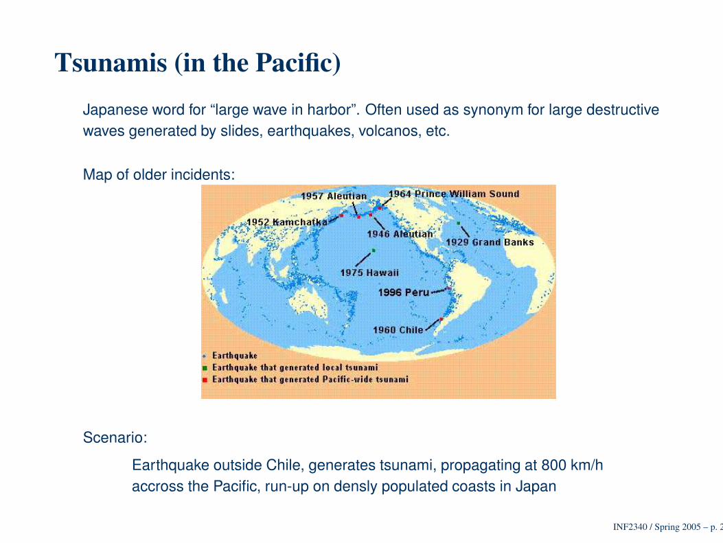
Tsunamis (in the Pacific)Japanese word for “large wave in harbor”. Often used as synonym for large destructivewaves generated by slides, earthquakes, volcanos, etc.

Map of older incidents:

Scenario:

Earthquake outside Chile, generates tsunami, propagating at 800 km/haccross the Pacific, run-up on densly populated coasts in Japan

INF2340 / Spring 2005 – p. 21

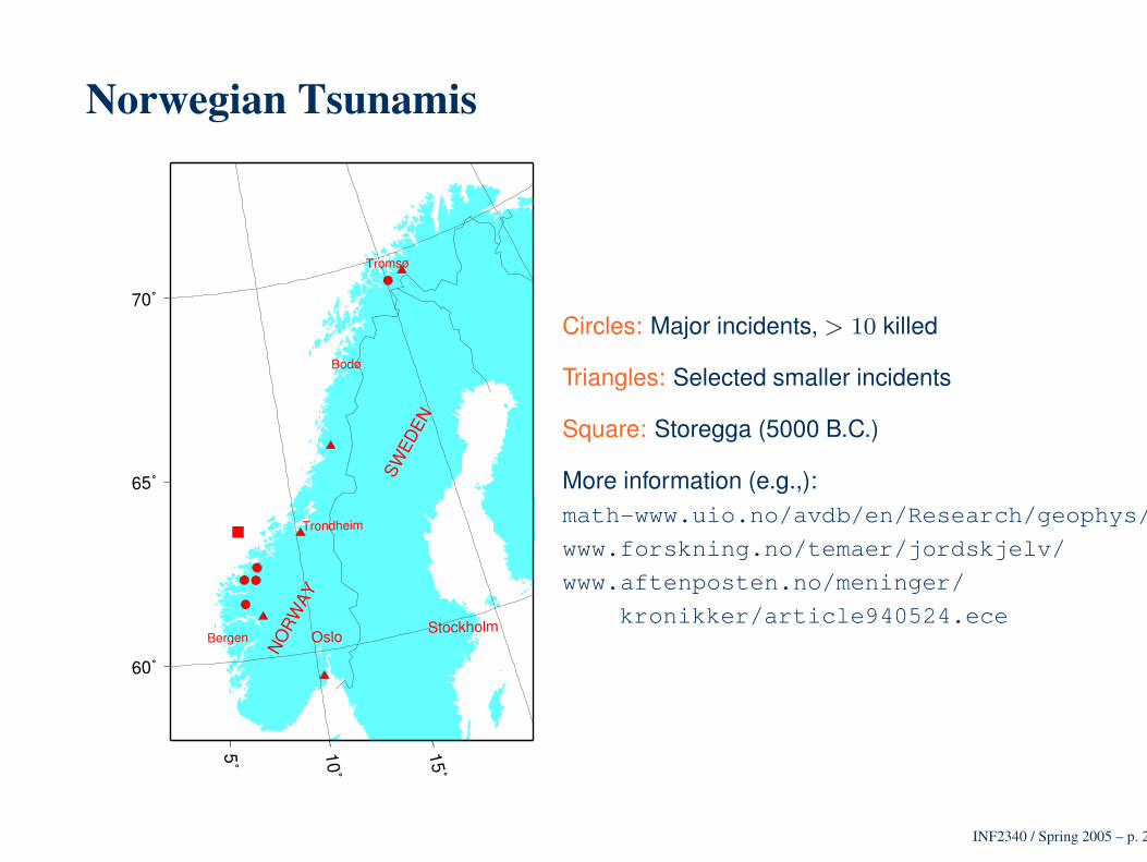
Norwegian Tsunamis

5˚ 10˚

15˚

60˚

65˚

70˚

Oslo StockholmBergen

Tromsø

Bodø

Trondheim

NO

RW

AY

SWED

EN

Circles: Major incidents, > 10 killed

Triangles: Selected smaller incidents

Square: Storegga (5000 B.C.)

More information (e.g.,):math-www.uio.no/avdb/en/Research/geophys/

www.forskning.no/temaer/jordskjelv/

www.aftenposten.no/meninger/

kronikker/article940524.ece

INF2340 / Spring 2005 – p. 22

Why Numerical Simulation?• Increase the understanding of tsunamis• Assist warning systems• Assist building of harbor protection (break waters)• Recognize critical coastal areas (e.g. move population)• Hindcast historical tsunamis (assist geologists)

INF2340 / Spring 2005 – p. 23

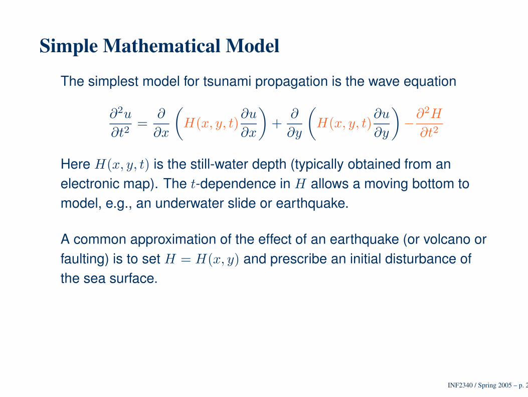
Simple Mathematical Model

The simplest model for tsunami propagation is the wave equation

∂2u

∂t2=

∂

∂x

(

H(x, y, t)∂u

∂x

)

+∂

∂y

(

H(x, y, t)∂u

∂y

)

−∂2H

∂t2

Here H(x, y, t) is the still-water depth (typically obtained from anelectronic map). The t-dependence in H allows a moving bottom tomodel, e.g., an underwater slide or earthquake.

A common approximation of the effect of an earthquake (or volcano orfaulting) is to set H = H(x, y) and prescribe an initial disturbance ofthe sea surface.

INF2340 / Spring 2005 – p. 24

First: the 1D Case

∂2u

∂t2=

∂

∂x

(

H(x)∂u

∂x

)

The term ∂∂x

(

H(x)∂u∂x

)

is common for many models of physicalphenomena

• Heat equation with spatially varying conductivity:ut = ∂

∂x

(

λ(x)∂u∂x

)

• Heat equation with temperature-dependent conductivity:ut = ∂

∂x

(

λ(u)∂u∂x

)

• Pressure distribution in a reservoir:cpt = ∂

∂x

(

K(x) ∂p∂x

)

• ....

INF2340 / Spring 2005 – p. 25

Discretisation• Two-step discretization, first outer operator

∂

∂x

(

H(x)∂u

∂x

)∣

∣

∣

x=xi

≈1

h

(

(

H∂u

∂x

)

∣

∣

∣

x=xi+1/2

−(

H∂u

∂x

)

∣

∣

∣

x=xi−1/2

)

• Then inner operator

(

H∂u

∂x

)

∣

∣

∣

x=xi+1/2

≈ Hi+1/2

ui+1 − ui

h

• And the overall discretization reads

∂

∂x

(

H∂u

∂x

)

≈Hi+1/2(ui+1 − ui)−Hi−1/2(ui − ui−1)

h2

INF2340 / Spring 2005 – p. 26

Discretisation, cont’d

Often the function H(x) is only given in the grid points, e.g., frommeasurements. Thus we need to define the value at the midpoint

• Arithmetic mean:

Hi+ 12

=1

2(Hi + Hi+1)

• Harmonic mean:

1

Hi+ 12

=1

2

(

1

Hi+

1

Hi+1

)

• Geometric mean:Hi+ 1

2= (HiHi+1)

1/2

INF2340 / Spring 2005 – p. 27

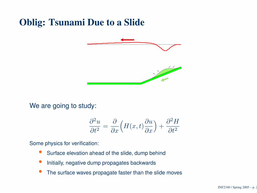
Oblig: Tsunami Due to a Slide

We are going to study:

∂2u

∂t2=

∂

∂x

(

H(x, t)∂u

∂x

)

+∂2H

∂t2

Some physics for verification:

• Surface elevation ahead of the slide, dump behind

• Initially, negative dump propagates backwards

• The surface waves propagate faster than the slide moves

INF2340 / Spring 2005 – p. 28

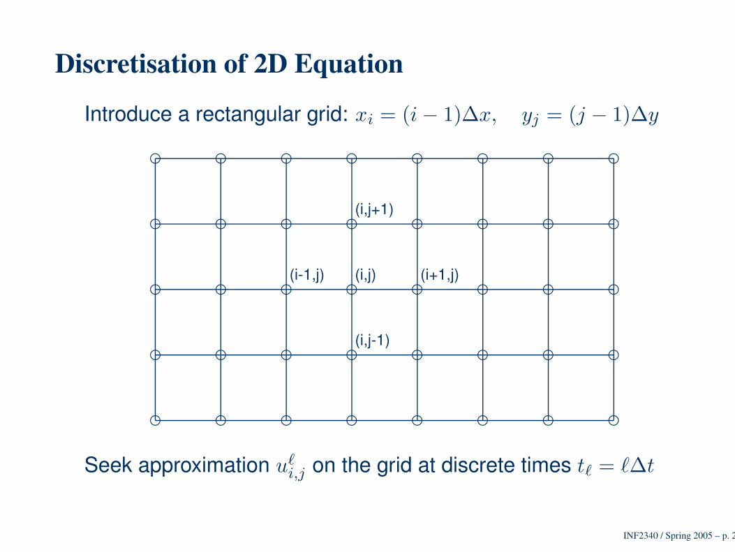
Discretisation of 2D Equation

Introduce a rectangular grid: xi = (i− 1)∆x, yj = (j − 1)∆y

d d d d d d d d

d d d d d d d d

d d d d d d d d

d d d d d d d d

d d d d d d d d

(i-1,j) (i,j) (i+1,j)

(i,j+1)

(i,j-1)

Seek approximation u`i,j on the grid at discrete times t` = `∆t

INF2340 / Spring 2005 – p. 29

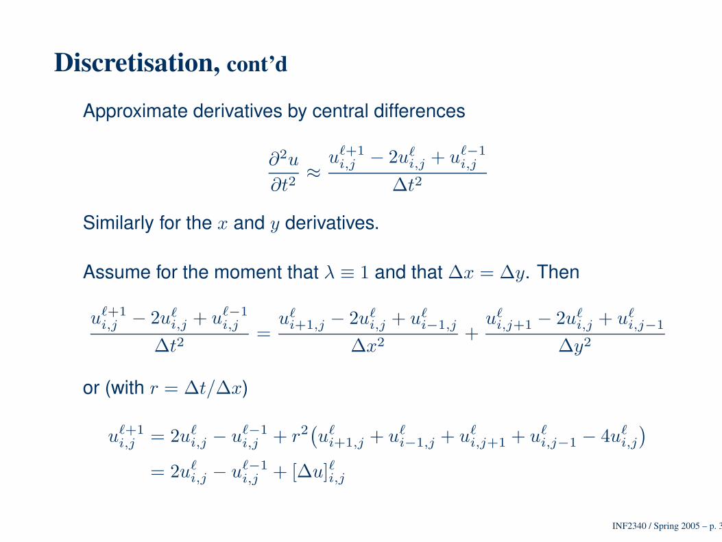
Discretisation, cont’d

Approximate derivatives by central differences

∂2u

∂t2≈

u`+1i,j − 2u`

i,j + u`−1i,j

∆t2

Similarly for the x and y derivatives.

Assume for the moment that λ ≡ 1 and that ∆x = ∆y. Then

u`+1i,j − 2u`

i,j + u`−1i,j

∆t2=

u`i+1,j − 2u`

i,j + u`i−1,j

∆x2+

u`i,j+1 − 2u`

i,j + u`i,j−1

∆y2

or (with r = ∆t/∆x)

u`+1i,j = 2u`

i,j − u`−1i,j + r2

(

u`i+1,j + u`

i−1,j + u`i,j+1 + u`

i,j−1 − 4u`i,j

)

= 2u`i,j − u`−1

i,j + [∆u]`i,j

INF2340 / Spring 2005 – p. 30

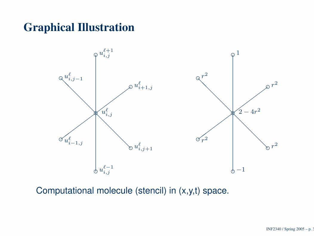
Graphical Illustration

c

c

c

c

c

c

c

@@

@@

@@

@@

@

u`i,j

u`+1

i,j

u`−1

i,j

u`i+1,j

u`i−1,j

u`i,j+1

u`i,j−1

c

c

c

c

c

c

c

@@

@@

@@

@@

@

2 − 4r2

1

−1

r2

r2

r2

r2

Computational molecule (stencil) in (x,y,t) space.

INF2340 / Spring 2005 – p. 31

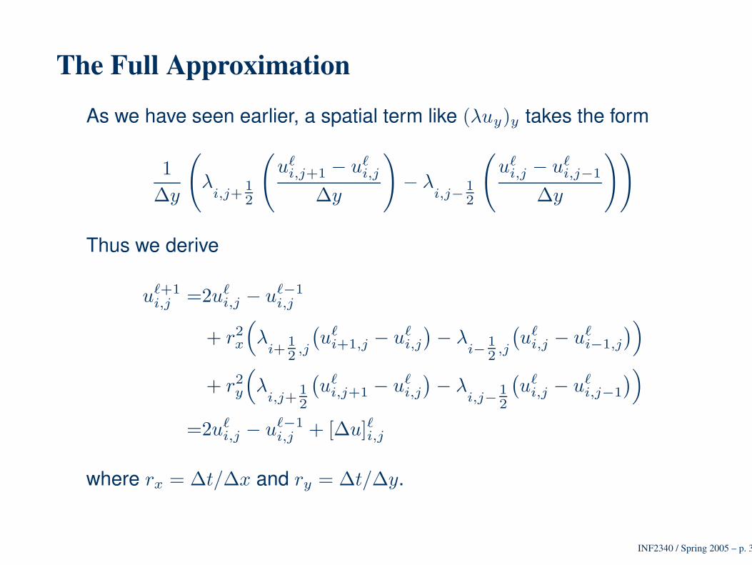
The Full Approximation

As we have seen earlier, a spatial term like (λuy)y takes the form

1

∆y

(

λi,j+

1

2

(

u`i,j+1 − u`

i,j

∆y

)

− λi,j−

1

2

(

u`i,j − u`

i,j−1

∆y

))

Thus we derive

u`+1i,j =2u`

i,j − u`−1i,j

+ r2x

(

λi+

1

2,j

(

u`i+1,j − u`

i,j

)

− λi−

1

2,j

(

u`i,j − u`

i−1,j

)

)

+ r2y

(

λi,j+

1

2

(

u`i,j+1 − u`

i,j

)

− λi,j−

1

2

(

u`i,j − u`

i,j−1

)

)

=2u`i,j − u`−1

i,j + [∆u]`i,j

where rx = ∆t/∆x and ry = ∆t/∆y.

INF2340 / Spring 2005 – p. 32

Boundary Conditions

For the 1-D wave equation we imposed u = 0 at the boundary.

Now, we would like to impose full reflection of waves like in a swimmingpool

∂u

∂n≡ ∇u · n = 0

Assume a rectangular domain. At the vertical (x =constant)boundaries the condition reads:

0 =∂u

∂n= ∇u · (±1, 0) = ±

∂u

∂x

Similarly at the horizontal boundaries (y =constant)

0 =∂u

∂n= ∇u · (0,±1) = ±

∂u

∂y

INF2340 / Spring 2005 – p. 33

Boundary Conditions, cont’d

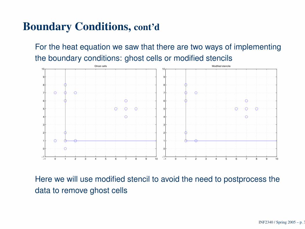
For the heat equation we saw that there are two ways of implementingthe boundary conditions: ghost cells or modified stencils

−1 0 1 2 3 4 5 6 7 8 9 10−1

0

1

2

3

4

5

6

7

8

9

10Ghost cells

−1 0 1 2 3 4 5 6 7 8 9 10−1

0

1

2

3

4

5

6

7

8

9

10Modified stencile

Here we will use modified stencil to avoid the need to postprocess thedata to remove ghost cells

INF2340 / Spring 2005 – p. 34

Solution Algorithm

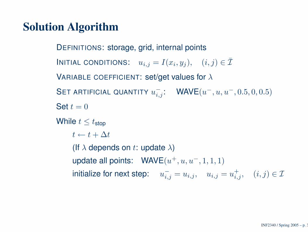
DEFINITIONS: storage, grid, internal points

INITIAL CONDITIONS: ui,j = I(xi, yj), (i, j) ∈ I

VARIABLE COEFFICIENT: set/get values for λ

SET ARTIFICIAL QUANTITY u−

i,j: WAVE(u−, u, u−, 0.5, 0, 0.5)

Set t = 0

While t ≤ tstop

t← t + ∆t

(If λ depends on t: update λ)

update all points: WAVE(u+, u, u−, 1, 1, 1)

initialize for next step: u−

i,j = ui,j, ui,j = u+i,j , (i, j) ∈ I

INF2340 / Spring 2005 – p. 35

Updating Internal and Boundary Points

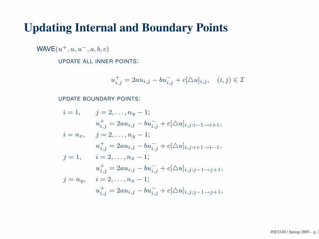
WAVE(u+, u, u−, a, b, c)

UPDATE ALL INNER POINTS:

u+

i,j = 2aui,j − bu−

i,j + c[4u]i,j , (i, j) ∈ I

UPDATE BOUNDARY POINTS:

i = 1, j = 2, . . . , ny − 1;

u+

i,j = 2aui,j − bu−

i,j + c[4u]i,j:i−1→i+1,

i = nx, j = 2, . . . , ny − 1;

u+

i,j = 2aui,j − bu−

i,j + c[4u]i,j:i+1→i−1,

j = 1, i = 2, . . . , nx − 1;

u+

i,j = 2aui,j − bu−

i,j + c[4u]i,j:j−1→j+1,

j = ny , i = 2, . . . , nx − 1;

u+

i,j = 2aui,j − bu−

i,j + c[4u]i,j:j−1→j+1,

INF2340 / Spring 2005 – p. 36

Updating Internal and Boundary Points, cont’d

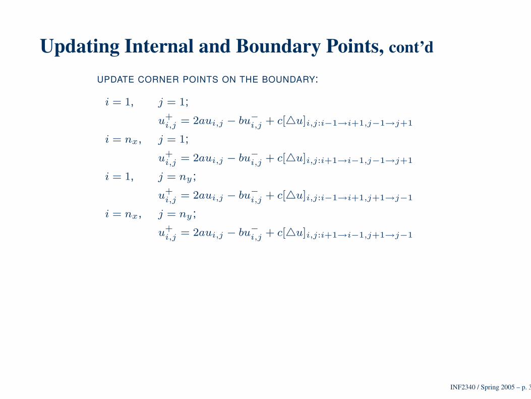
UPDATE CORNER POINTS ON THE BOUNDARY:

i = 1, j = 1;

u+

i,j = 2aui,j − bu−

i,j + c[4u]i,j:i−1→i+1,j−1→j+1

i = nx, j = 1;

u+

i,j = 2aui,j − bu−

i,j + c[4u]i,j:i+1→i−1,j−1→j+1

i = 1, j = ny ;

u+

i,j = 2aui,j − bu−

i,j + c[4u]i,j:i−1→i+1,j+1→j−1

i = nx, j = ny ;

u+

i,j = 2aui,j − bu−

i,j + c[4u]i,j:i+1→i−1,j+1→j−1

INF2340 / Spring 2005 – p. 37

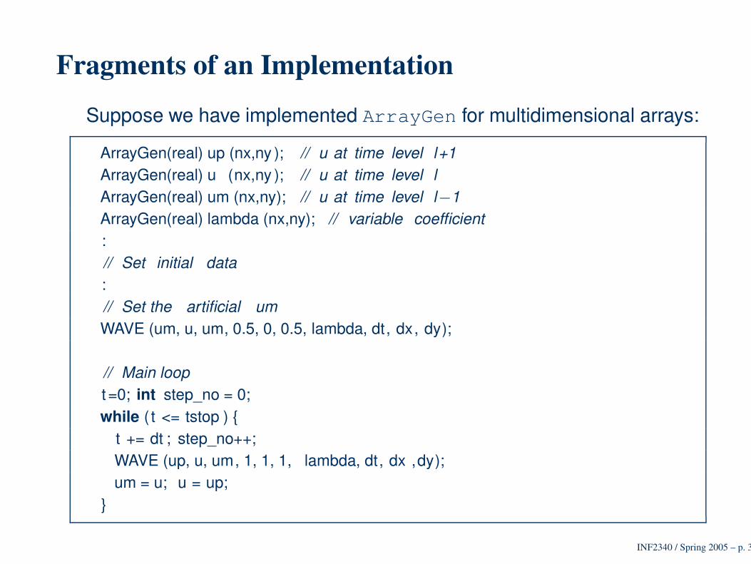
Fragments of an Implementation

Suppose we have implemented ArrayGen for multidimensional arrays:

ArrayGen(real) up (nx,ny ); // u at time level l+1ArrayGen(real) u (nx,ny ); // u at time level lArrayGen(real) um (nx,ny); // u at time level l−1ArrayGen(real) lambda (nx,ny); // variable coefficient:// Set initial data:// Set the artificial umWAVE (um, u, um, 0.5, 0, 0.5, lambda, dt, dx, dy);

// Main loopt =0; int step_no = 0;while ( t <= tstop )

t += dt ; step_no++;WAVE (up, u, um, 1, 1, 1, lambda, dt, dx ,dy);um = u; u = up;

INF2340 / Spring 2005 – p. 38

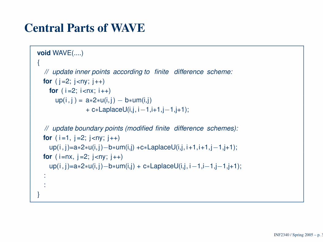
Central Parts of WAVE

void WAVE(....)

// update inner points according to finite difference scheme:for ( j =2; j<ny; j++)

for ( i =2; i<nx; i++)up(i , j ) = a∗2∗u(i, j ) − b∗um(i,j)

+ c∗LaplaceU(i,j, i−1,i+1,j−1,j+1);

// update boundary points (modified finite difference schemes):for ( i =1, j =2; j<ny; j++)

up(i , j )=a∗2∗u(i, j )−b∗um(i,j) +c∗LaplaceU(i,j, i+1,i+1,j−1,j+1);for ( i=nx, j =2; j<ny; j++)

up(i , j )=a∗2∗u(i, j )−b∗um(i,j) + c∗LaplaceU(i,j, i−1,i−1,j−1,j+1);::

INF2340 / Spring 2005 – p. 39

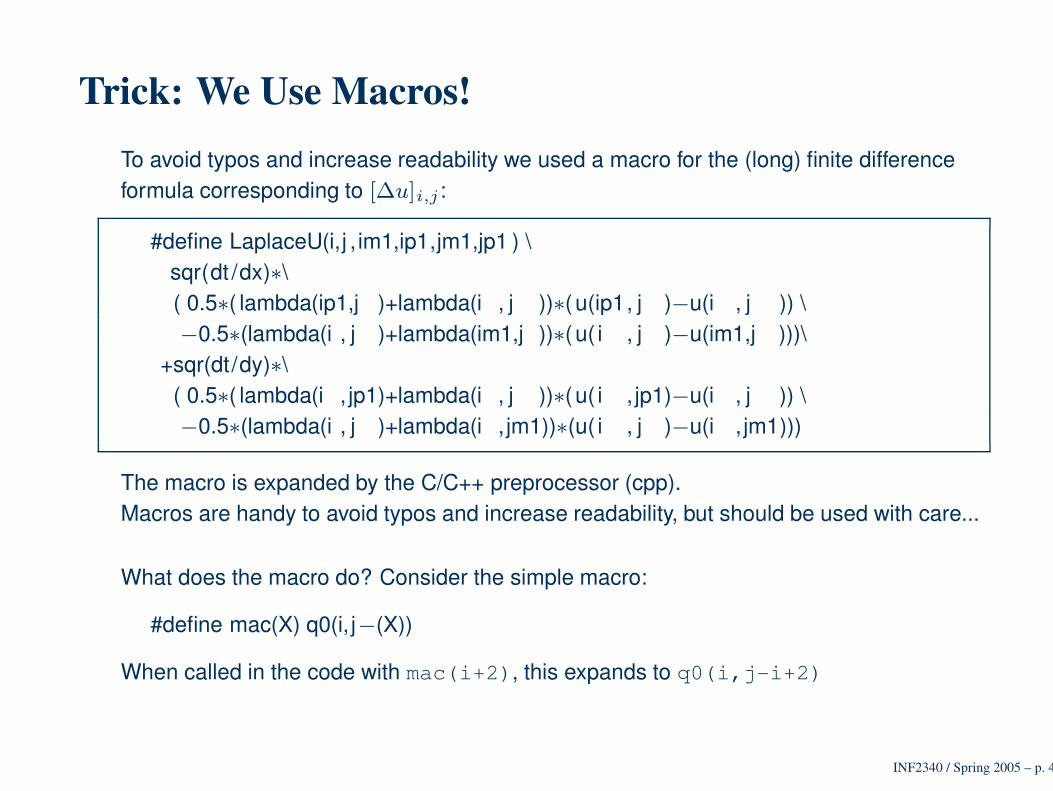
Trick: We Use Macros!To avoid typos and increase readability we used a macro for the (long) finite differenceformula corresponding to [∆u]i,j :

#define LaplaceU(i,j , im1,ip1,jm1,jp1 ) \sqr(dt /dx)∗\( 0.5∗( lambda(ip1,j )+lambda(i , j ))∗(u(ip1, j )−u(i , j )) \−0.5∗(lambda(i , j )+lambda(im1,j ))∗(u( i , j )−u(im1,j )))\

+sqr(dt/dy)∗\( 0.5∗( lambda(i , jp1)+lambda(i , j ))∗(u( i , jp1)−u(i , j )) \−0.5∗(lambda(i , j )+lambda(i , jm1))∗(u( i , j )−u(i , jm1)))

The macro is expanded by the C/C++ preprocessor (cpp).Macros are handy to avoid typos and increase readability, but should be used with care...

What does the macro do? Consider the simple macro:

#define mac(X) q0(i, j−(X))

When called in the code with mac(i+2), this expands to q0(i,j-i+2)

INF2340 / Spring 2005 – p. 40

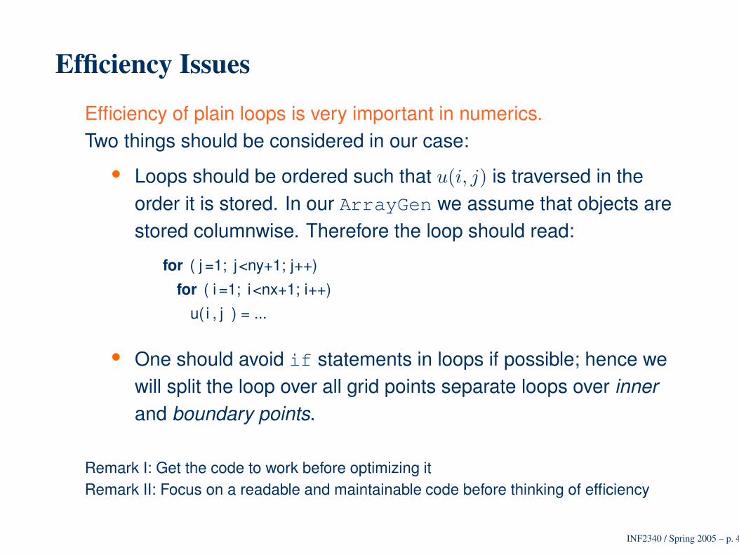
Efficiency Issues

Efficiency of plain loops is very important in numerics.Two things should be considered in our case:

• Loops should be ordered such that u(i, j) is traversed in theorder it is stored. In our ArrayGen we assume that objects arestored columnwise. Therefore the loop should read:

for ( j =1; j<ny+1; j++)

for ( i =1; i<nx+1; i++)

u( i , j ) = ...

• One should avoid if statements in loops if possible; hence wewill split the loop over all grid points separate loops over innerand boundary points.

Remark I: Get the code to work before optimizing itRemark II: Focus on a readable and maintainable code before thinking of efficiency

INF2340 / Spring 2005 – p. 41

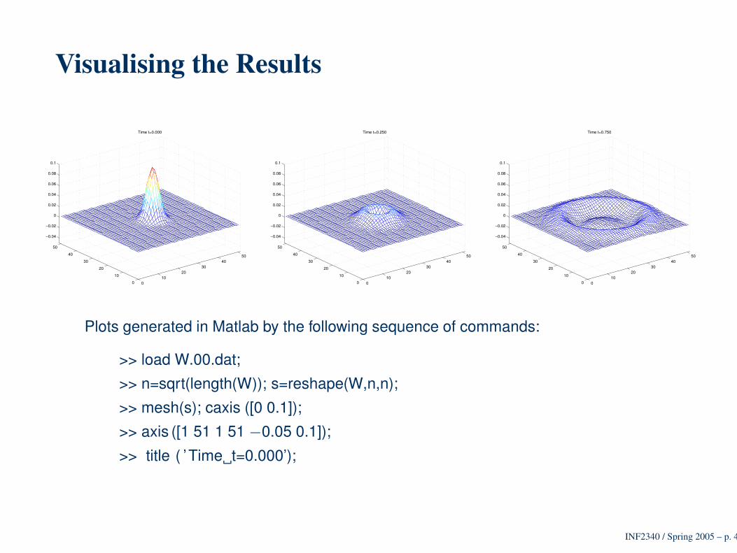
Visualising the Results

010

2030

4050

0

10

20

30

40

50

−0.04

−0.02

0

0.02

0.04

0.06

0.08

0.1

Time t=0.000

010

2030

4050

0

10

20

30

40

50

−0.04

−0.02

0

0.02

0.04

0.06

0.08

0.1

Time t=0.250

010

2030

4050

0

10

20

30

40

50

−0.04

−0.02

0

0.02

0.04

0.06

0.08

0.1

Time t=0.750

Plots generated in Matlab by the following sequence of commands:

>> load W.00.dat;

>> n=sqrt(length(W)); s=reshape(W,n,n);

>> mesh(s); caxis ([0 0.1]);

>> axis ([1 51 1 51 −0.05 0.1]);

>> title ( ’Time t=0.000’);

INF2340 / Spring 2005 – p. 42

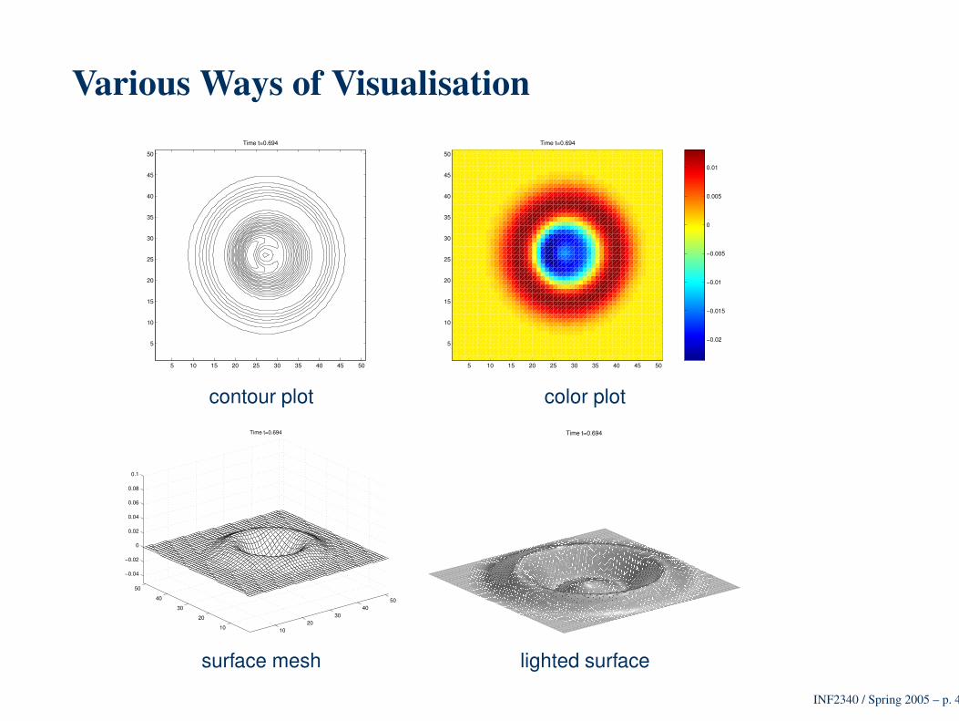
Various Ways of Visualisation

5 10 15 20 25 30 35 40 45 50

5

10

15

20

25

30

35

40

45

50

Time t=0.694

5 10 15 20 25 30 35 40 45 50

5

10

15

20

25

30

35

40

45

50

Time t=0.694

−0.02

−0.015

−0.01

−0.005

0

0.005

0.01

contour plot color plot

1020

3040

50

10

20

30

40

50

−0.04

−0.02

0

0.02

0.04

0.06

0.08

0.1

Time t=0.694 Time t=0.694

surface mesh lighted surface

INF2340 / Spring 2005 – p. 43

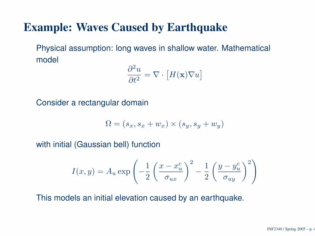
Example: Waves Caused by Earthquake

Physical assumption: long waves in shallow water. Mathematicalmodel

∂2u

∂t2= ∇ ·

[

H(x)∇u]

Consider a rectangular domain

Ω = (sx, sx + wx)× (sy, sy + wy)

with initial (Gaussian bell) function

I(x, y) = Au exp

(

−1

2

(

x− xcu

σux

)2

−1

2

(

y − ycu

σuy

)2)

This models an initial elevation caused by an earthquake.

INF2340 / Spring 2005 – p. 44

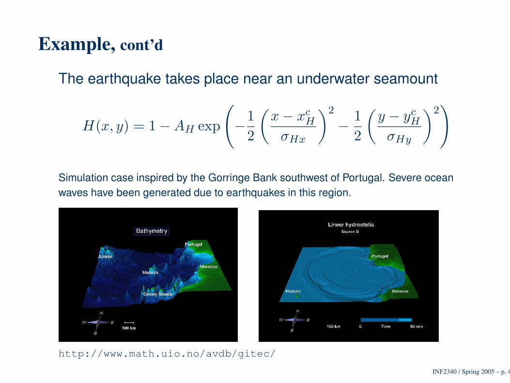
Example, cont’d

The earthquake takes place near an underwater seamount

H(x, y) = 1−AH exp

(

−1

2

(

x− xcH

σHx

)2

−1

2

(

y − ycH

σHy

)2)

Simulation case inspired by the Gorringe Bank southwest of Portugal. Severe oceanwaves have been generated due to earthquakes in this region.

http://www.math.uio.no/avdb/gitec/

INF2340 / Spring 2005 – p. 45

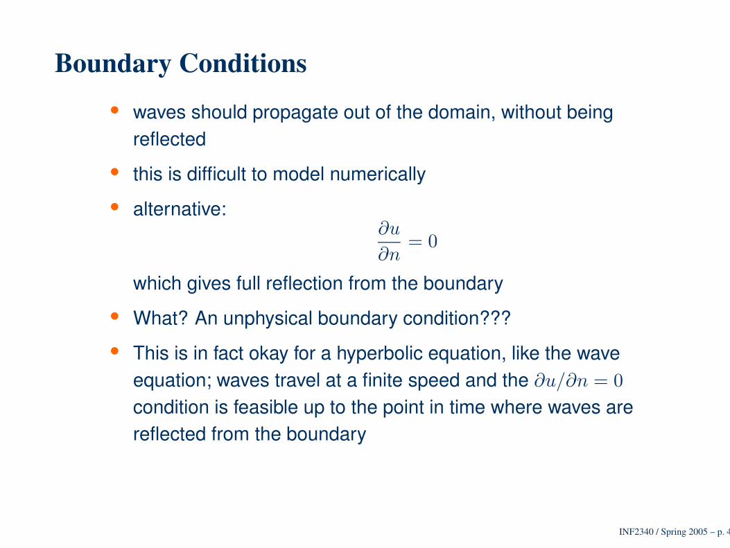
Boundary Conditions• waves should propagate out of the domain, without being

reflected

• this is difficult to model numerically

• alternative:∂u

∂n= 0

which gives full reflection from the boundary

• What? An unphysical boundary condition???

• This is in fact okay for a hyperbolic equation, like the waveequation; waves travel at a finite speed and the ∂u/∂n = 0

condition is feasible up to the point in time where waves arereflected from the boundary

INF2340 / Spring 2005 – p. 46

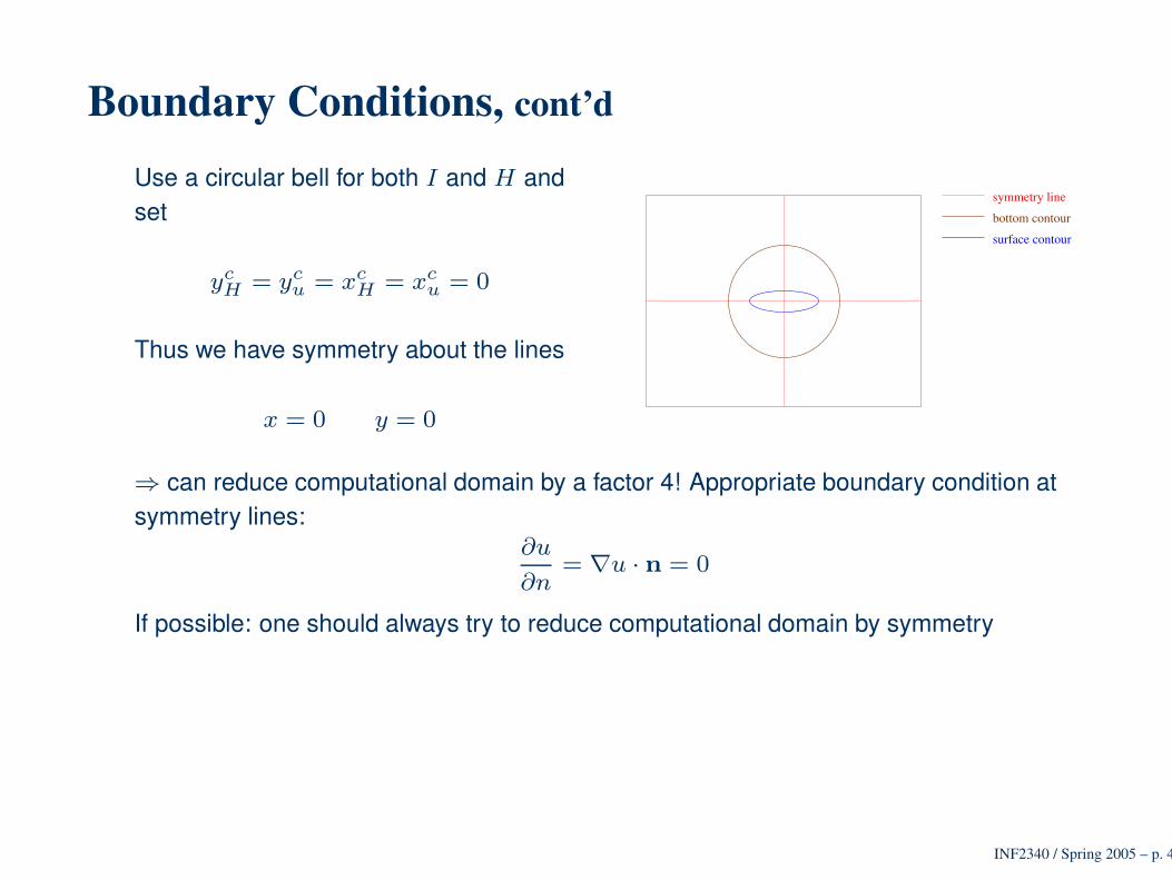
Boundary Conditions, cont’d

Use a circular bell for both I and H andset

ycH = yc

u = xcH = xc

u = 0

Thus we have symmetry about the lines

x = 0 y = 0

surface contour

bottom contour

symmetry line

⇒ can reduce computational domain by a factor 4! Appropriate boundary condition atsymmetry lines:

∂u

∂n= ∇u · n = 0

If possible: one should always try to reduce computational domain by symmetry

INF2340 / Spring 2005 – p. 47

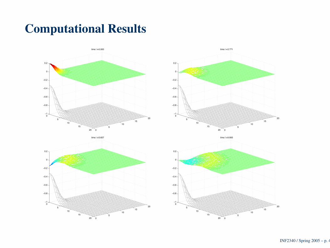
Computational Results

0

5

10

15

20 05

1015

20

−1

−0.8

−0.6

−0.4

−0.2

0

0.2

time: t=0.000

0

5

10

15

20 05

1015

20

−1

−0.8

−0.6

−0.4

−0.2

0

0.2

time: t=3.771

0

5

10

15

20 05

1015

20

−1

−0.8

−0.6

−0.4

−0.2

0

0.2

time: t=5.657

0

5

10

15

20 05

1015

20

−1

−0.8

−0.6

−0.4

−0.2

0

0.2

time: t=9.900

INF2340 / Spring 2005 – p. 48