Recap Lecture + Thomson Scattering

Thermal radiationBlackbody radiation

Bremsstrahlung radiation

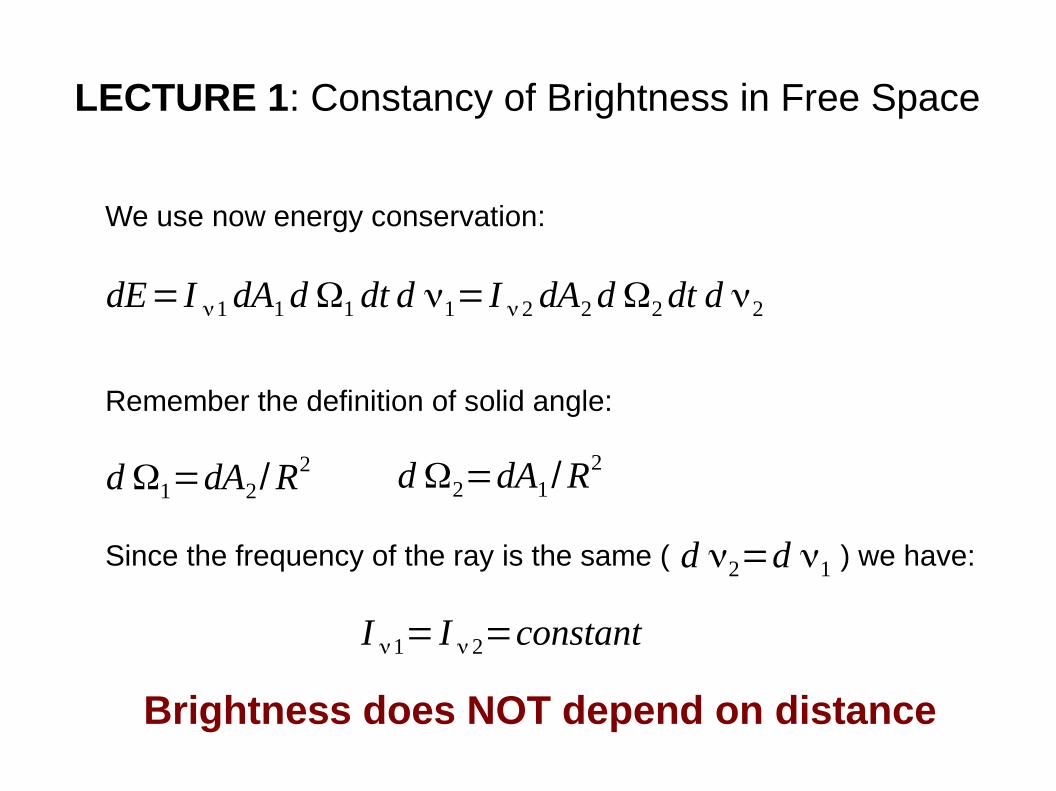
LECTURE 1: Constancy of Brightness in Free Space

We use now energy conservation:

dE=I ν1 dA1 d Ω1 dt d ν1=I ν 2 dA2 d Ω2 dt d ν2

Remember the definition of solid angle:

d Ω1=dA2/R2 d Ω2=dA1/R

2

Since the frequency of the ray is the same ( ) we have:d ν2=d ν1

I ν1= I ν 2=constant

Brightness does NOT depend on distance

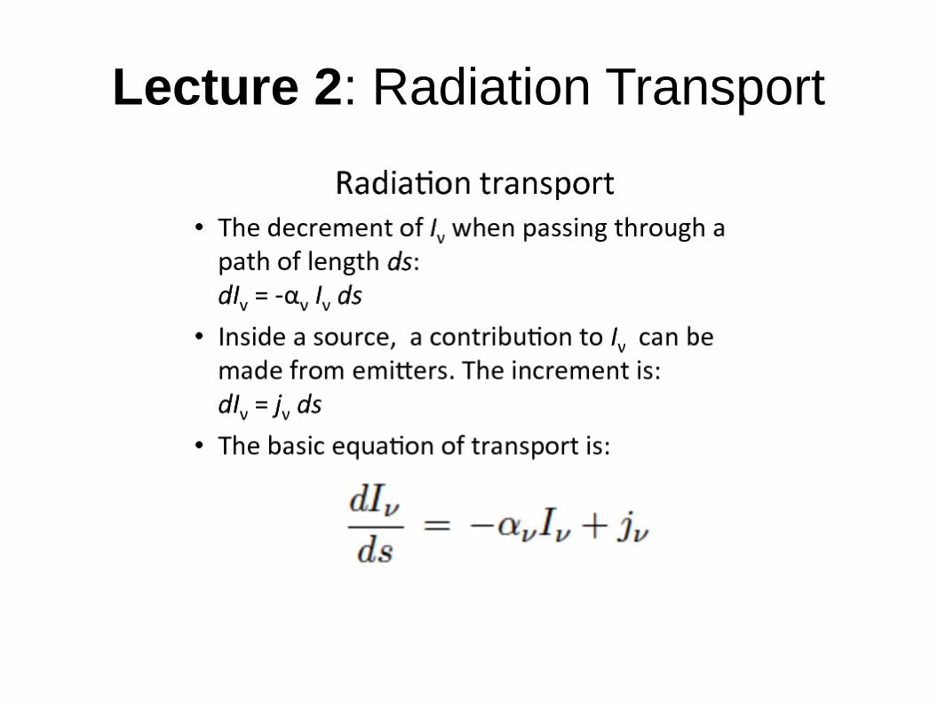
Lecture 2: Radiation Transport

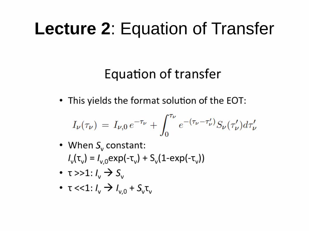
Lecture 2: Equation of Transfer

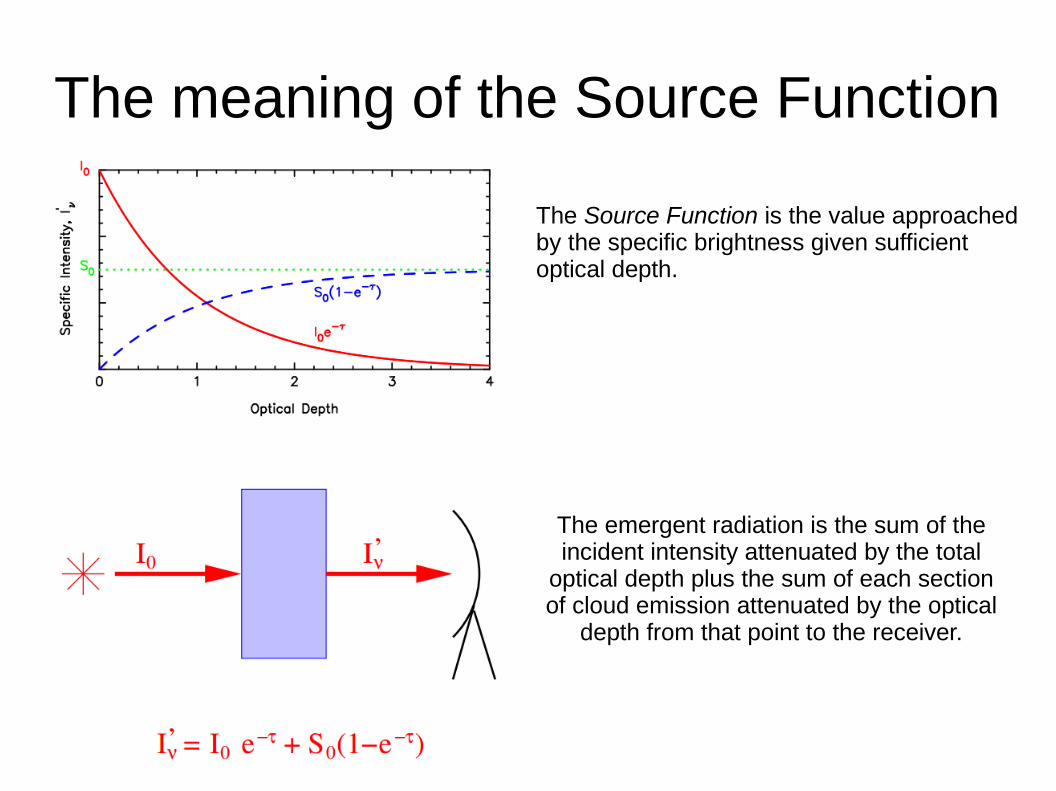
The meaning of the Source Function

The Source Function is the value approached by the specific brightness given sufficient optical depth.

The emergent radiation is the sum of the incident intensity attenuated by the total

optical depth plus the sum of each section of cloud emission attenuated by the optical

depth from that point to the receiver.

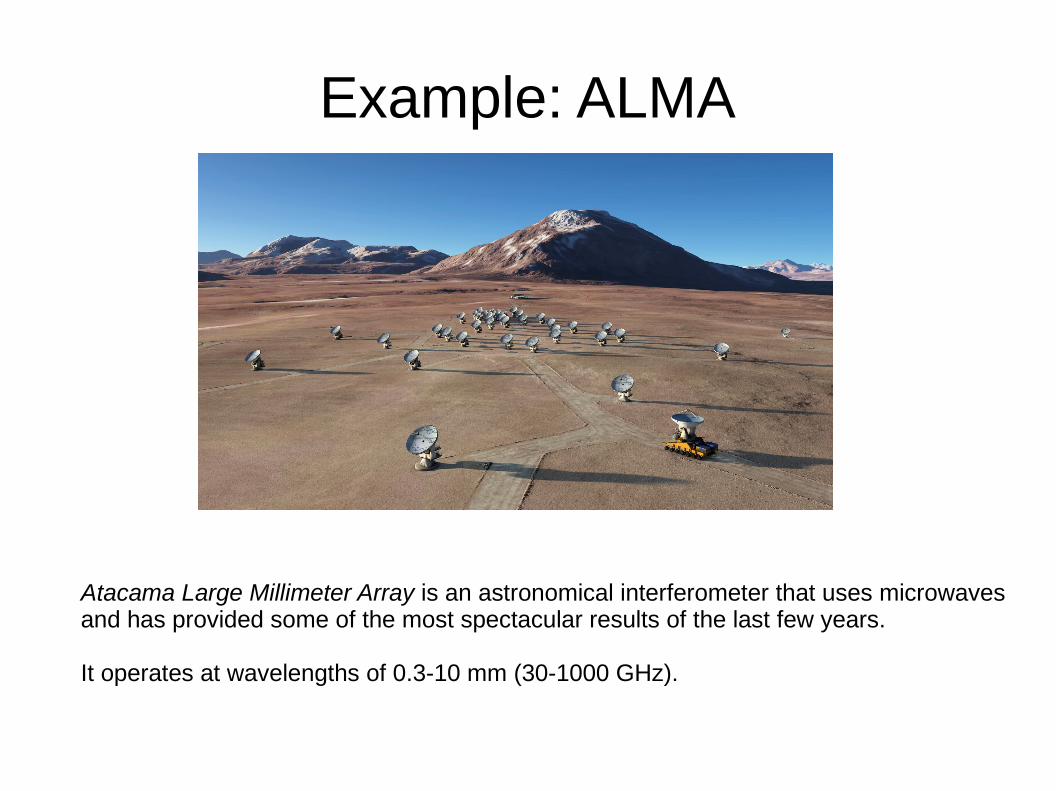
Example: ALMA

Atacama Large Millimeter Array is an astronomical interferometer that uses microwavesand has provided some of the most spectacular results of the last few years.

It operates at wavelengths of 0.3-10 mm (30-1000 GHz).

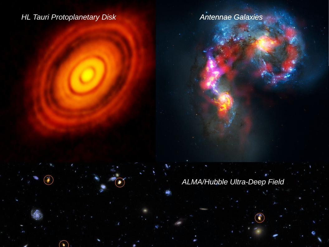
Antennae GalaxiesAntennae GalaxiesHL Tauri Protoplanetary Disk

ALMA/Hubble Ultra-Deep Field

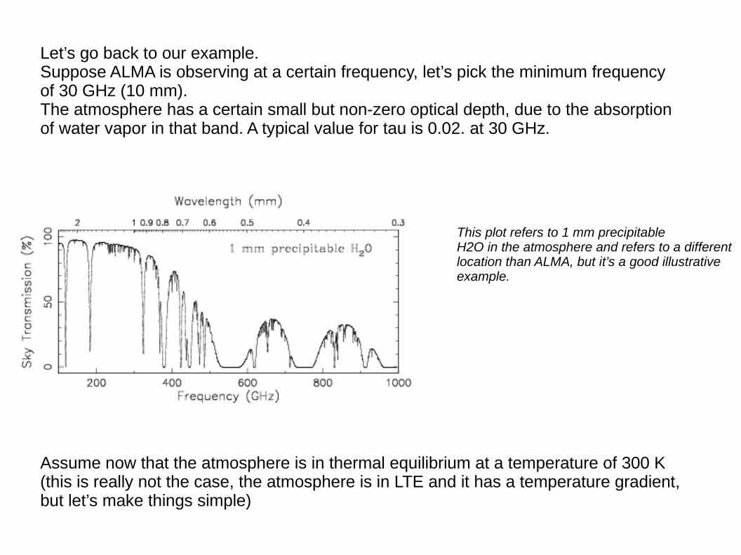
Let’s go back to our example. Suppose ALMA is observing at a certain frequency, let’s pick the minimum frequencyof 30 GHz (10 mm). The atmosphere has a certain small but non-zero optical depth, due to the absorptionof water vapor in that band. A typical value for tau is 0.02. at 30 GHz.

This plot refers to 1 mm precipitableH2O in the atmosphere and refers to a differentlocation than ALMA, but it’s a good illustrativeexample.

Assume now that the atmosphere is in thermal equilibrium at a temperature of 300 K(this is really not the case, the atmosphere is in LTE and it has a temperature gradient, but let’s make things simple)

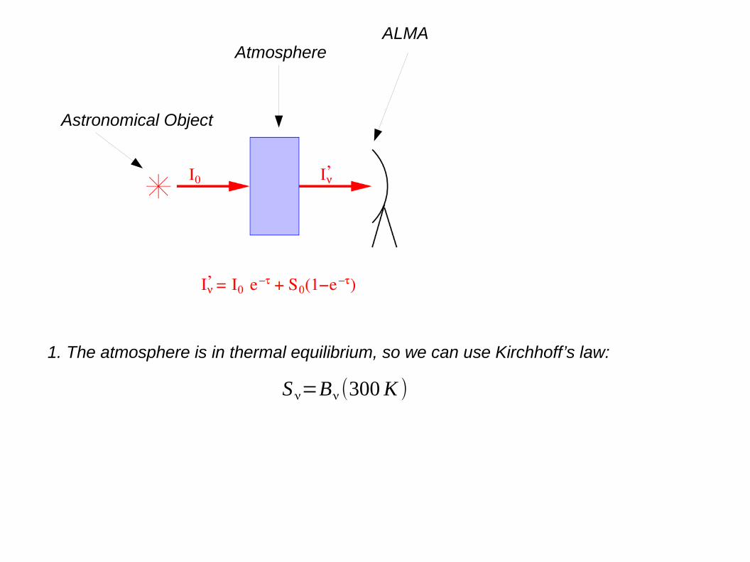
ALMAAtmosphere

Astronomical Object

1. The atmosphere is in thermal equilibrium, so we can use Kirchhoff’s law:

Sν=Bν(300 K )

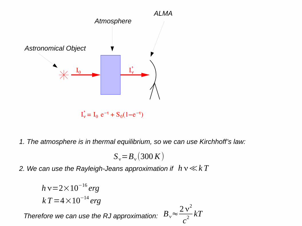
ALMAAtmosphere

Astronomical Object

1. The atmosphere is in thermal equilibrium, so we can use Kirchhoff’s law:

Sν=Bν(300 K )

2. We can use the Rayleigh-Jeans approximation if h ν≪k T

h ν=2×10−16 erg

k T =4×10−14 erg

Therefore we can use the RJ approximation: Bν≈2ν2

c2 kT

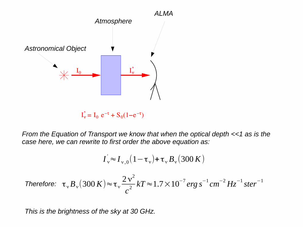
ALMAAtmosphere

Astronomical Object

I ν' ≈ I ν ,0(1−τν)+τν Bν(300 K )

From the Equation of Transport we know that when the optical depth <<1 as is thecase here, we can rewrite to first order the above equation as:

Therefore: τν Bν(300 K )≈τν

2ν2

c2 kT≈1.7×10−7 erg s−1 cm−2 Hz−1 ster−1

This is the brightness of the sky at 30 GHz.

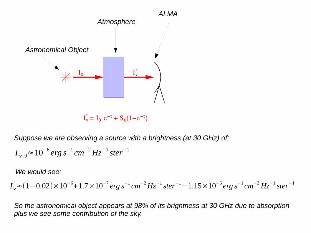
ALMAAtmosphere

Astronomical Object

Suppose we are observing a source with a brightness (at 30 GHz) of:

I ν , 0≈10−6 erg s−1 cm−2 Hz−1 ster−1

We would see:

I ν' ≈(1−0.02)×10−6+1.7×10−7 erg s−1 cm−2 Hz−1 ster−1=1.15×10−6 erg s−1 cm−2 Hz−1 ster−1

So the astronomical object appears at 98% of its brightness at 30 GHz due to absorptionplus we see some contribution of the sky.

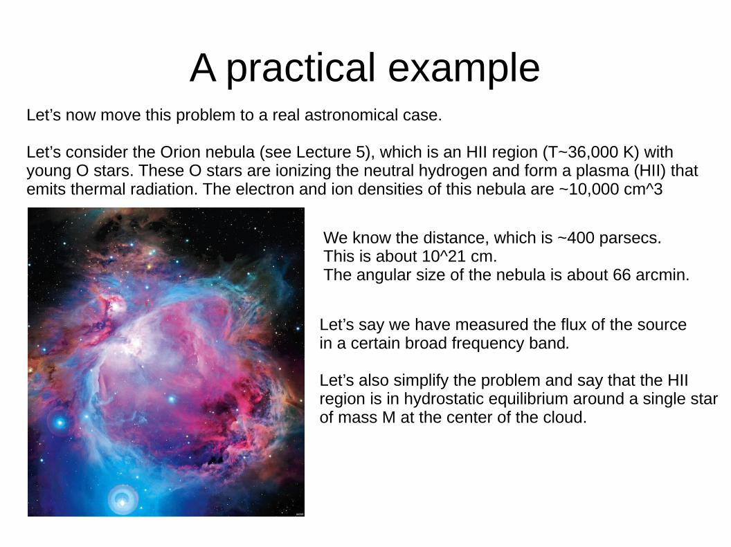
A practical exampleLet’s now move this problem to a real astronomical case.

Let’s consider the Orion nebula (see Lecture 5), which is an HII region (T~36,000 K) with young O stars. These O stars are ionizing the neutral hydrogen and form a plasma (HII) that emits thermal radiation. The electron and ion densities of this nebula are ~10,000 cm^3

We know the distance, which is ~400 parsecs. This is about 10^21 cm. The angular size of the nebula is about 66 arcmin.

Let’s say we have measured the flux of the sourcein a certain broad frequency band.

Let’s also simplify the problem and say that the HII region is in hydrostatic equilibrium around a single starof mass M at the center of the cloud.

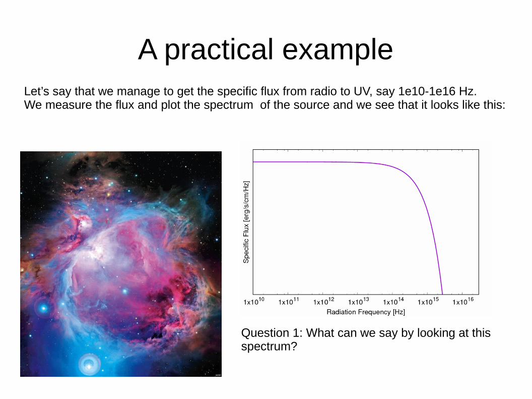
A practical exampleLet’s say that we manage to get the specific flux from radio to UV, say 1e10-1e16 Hz. We measure the flux and plot the spectrum of the source and we see that it looks like this:

Question 1: What can we say by looking at this spectrum?

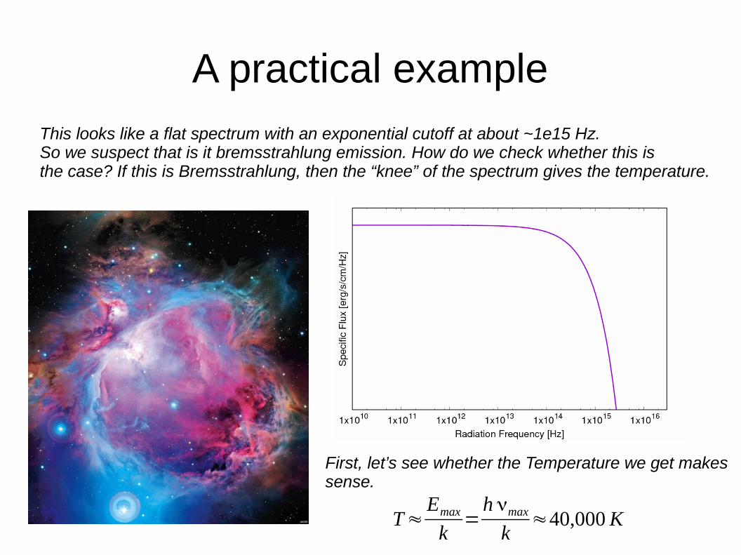
A practical exampleThis looks like a flat spectrum with an exponential cutoff at about ~1e15 Hz. So we suspect that is it bremsstrahlung emission. How do we check whether this is the case? If this is Bremsstrahlung, then the “knee” of the spectrum gives the temperature.

First, let’s see whether the Temperature we get makessense.

T≈Emax

k=

h νmax

k≈40,000 K

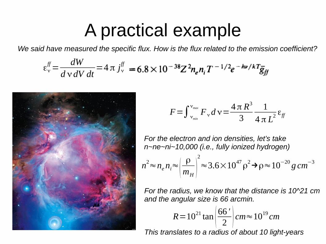
A practical exampleWe said have measured the specific flux. How is the flux related to the emission coefficient?

ενff=

dWd νdV dt

=4 π jνff

F=∫νmin

νmax

F ν d ν=4π R3

31

4 π L2 εff

For the electron and ion densities, let’s take n~ne~ni~10,000 (i.e., fully ionized hydrogen)

For the radius, we know that the distance is 10^21 cmand the angular size is 66 arcmin.

This translates to a radius of about 10 light-years

R=1021 tan ( 66 '2 ) cm≈1019 cm

n2≈ne ni≈ (

ρ

mH )2

≈3.6×1047ρ

2→ρ≈10−20 g cm−3

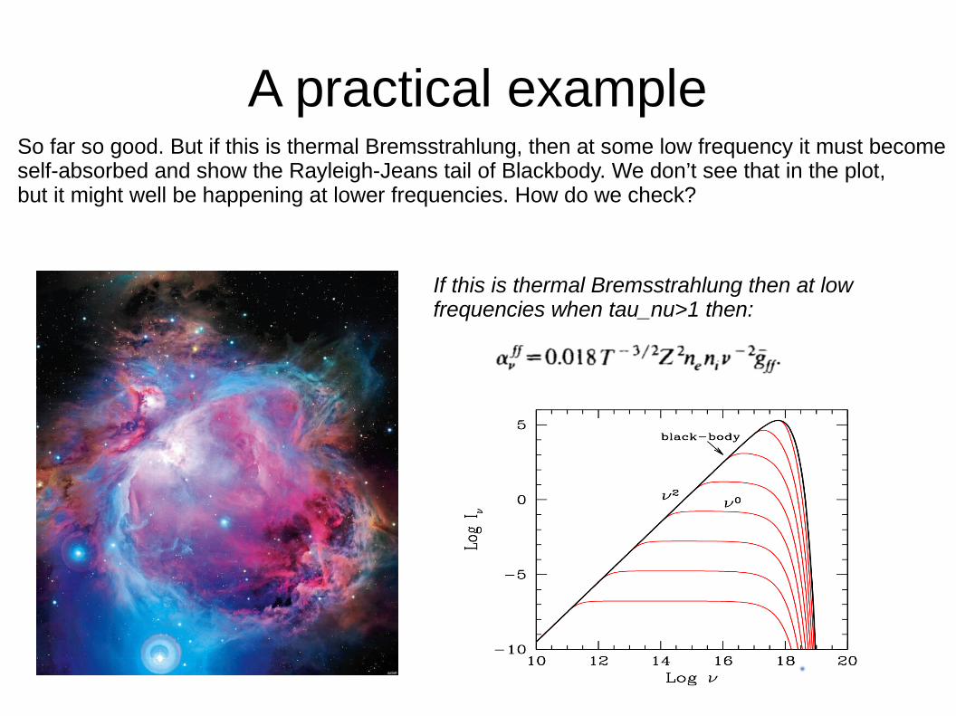
A practical exampleSo far so good. But if this is thermal Bremsstrahlung, then at some low frequency it must become self-absorbed and show the Rayleigh-Jeans tail of Blackbody. We don’t see that in the plot, but it might well be happening at lower frequencies. How do we check?

If this is thermal Bremsstrahlung then at low frequencies when tau_nu>1 then:

A practical example

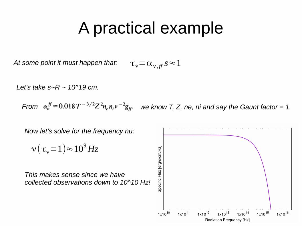
τν=αν , ff s≈1At some point it must happen that:

Let’s take s~R ~ 10^19 cm.

From we know T, Z, ne, ni and say the Gaunt factor = 1.

Now let’s solve for the frequency nu:

ν( τν=1)≈109 Hz

This makes sense since we havecollected observations down to 10^10 Hz!

A practical example

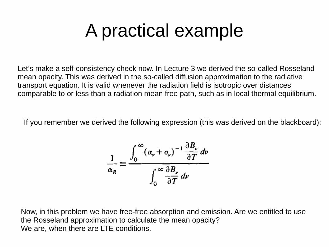
Let’s make a self-consistency check now. In Lecture 3 we derived the so-called Rosselandmean opacity. This was derived in the so-called diffusion approximation to the radiative transport equation. It is valid whenever the radiation field is isotropic over distances comparable to or less than a radiation mean free path, such as in local thermal equilibrium.

If you remember we derived the following expression (this was derived on the blackboard):

Now, in this problem we have free-free absorption and emission. Are we entitled to usethe Rosseland approximation to calculate the mean opacity? We are, when there are LTE conditions.

A practical example

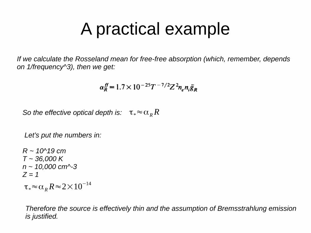
If we calculate the Rosseland mean for free-free absorption (which, remember, dependson 1/frequency^3), then we get:

So the effective optical depth is: τ*≈αR R

Let’s put the numbers in:

R ~ 10^19 cmT ~ 36,000 Kn ~ 10,000 cm^-3Z = 1

τ*≈αR R≈2×10−14

Therefore the source is effectively thin and the assumption of Bremsstrahlung emissionis justified.

Is this all?

To calculate the opacity of a source we have to consider all processes that might beongoing and calculate the total opacity due to each single process. Then we can say whether the source is optically thin or thick.

Here we are considering a plasma (HII region) and we have checked that the Bremsstrahlungabsorption is negligible.

But is this it? What else might be ongoing?

If the radiation in the cloud interacts with the electrons then it might simply “bounce off” the electrons and change direction. This is called electron scattering and in the lowenergy limit (h nu <<kT) it is called Thomson scattering. At high energies things change a bit and we will discuss this in the future (Compton scattering).

Let’s check whether the cloud is optically thinwhen considering electron scattering too.

So first let’s understand what is electron scattering

Thomson Scattering

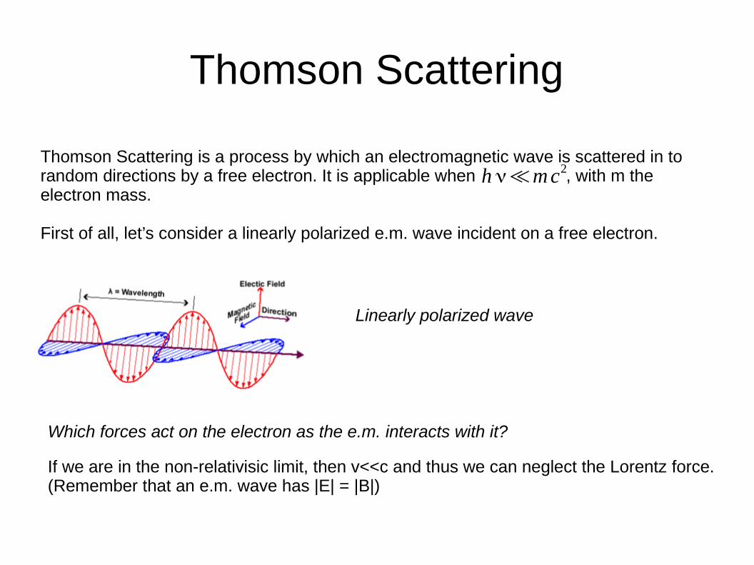
Thomson Scattering is a process by which an electromagnetic wave is scattered in to random directions by a free electron. It is applicable when , with m the electron mass.

First of all, let’s consider a linearly polarized e.m. wave incident on a free electron.

h ν≪mc2

Linearly polarized wave

If we are in the non-relativisic limit, then v<<c and thus we can neglect the Lorentz force. (Remember that an e.m. wave has |E| = |B|)

Which forces act on the electron as the e.m. interacts with it?

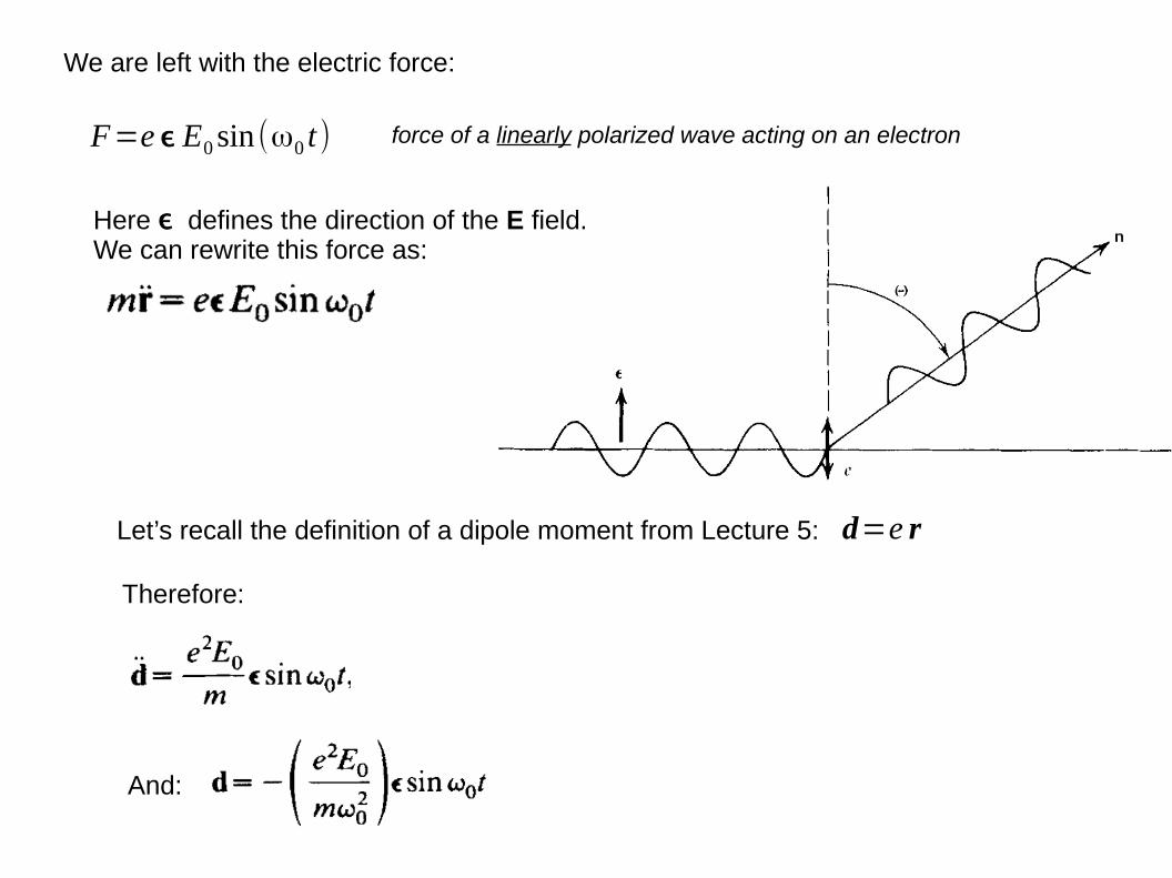
We are left with the electric force:

F=e ϵ E0 sin(ω0 t ) force of a linearly polarized wave acting on an electron

Here defines the direction of the E field. We can rewrite this force as:

ϵ

Let’s recall the definition of a dipole moment from Lecture 5: d=e r

Therefore:

And:

We are left with the electric force:

F=e ϵ E0 sin(ω0 t ) force of a linearly polarized wave acting on an electron

Here defines the direction of the E field. We can rewrite this force as:

ϵ

Let’s recall the definition of a dipole moment from Lecture 5: d=e r

Therefore:

And:

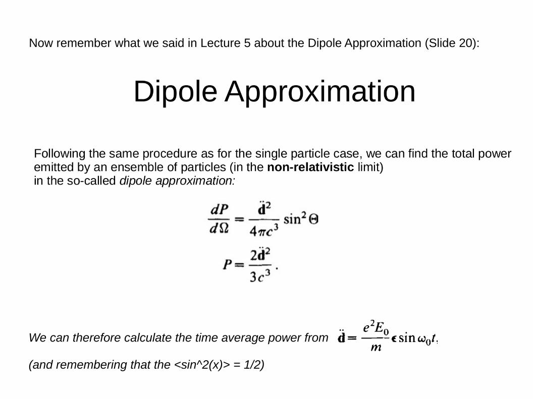
Now remember what we said in Lecture 5 about the Dipole Approximation (Slide 20):

We can therefore calculate the time average power from

(and remembering that the <sin^2(x)> = 1/2)

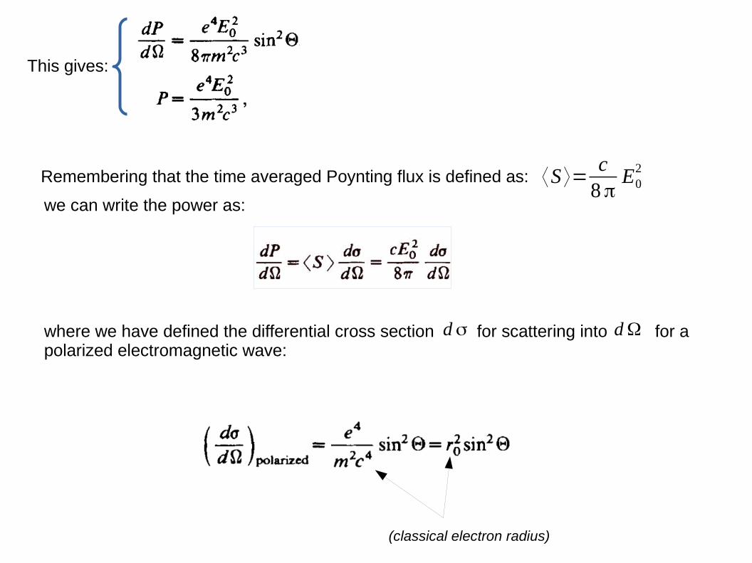
This gives:

Remembering that the time averaged Poynting flux is defined as: ⟨S ⟩=c

8πE0

2

we can write the power as:

where we have defined the differential cross section for scattering into for a polarized electromagnetic wave:

d σ d Ω

(classical electron radius)

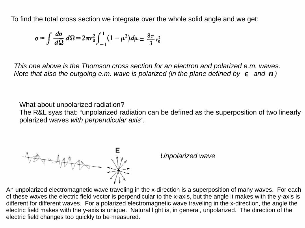
Unpolarized wave

An unpolarized electromagnetic wave traveling in the x-direction is a superposition of many waves. For each of these waves the electric field vector is perpendicular to the x-axis, but the angle it makes with the y-axis is different for different waves. For a polarized electromagnetic wave traveling in the x-direction, the angle the electric field makes with the y-axis is unique. Natural light is, in general, unpolarized. The direction of the electric field changes too quickly to be measured.

To find the total cross section we integrate over the whole solid angle and we get:

=

This one above is the Thomson cross section for an electron and polarized e.m. waves.Note that also the outgoing e.m. wave is polarized (in the plane defined by and )ϵ n

What about unpolarized radiation? The R&L syas that: “unpolarized radiation can be defined as the superposition of two linearly polarized waves with perpendicular axis”.

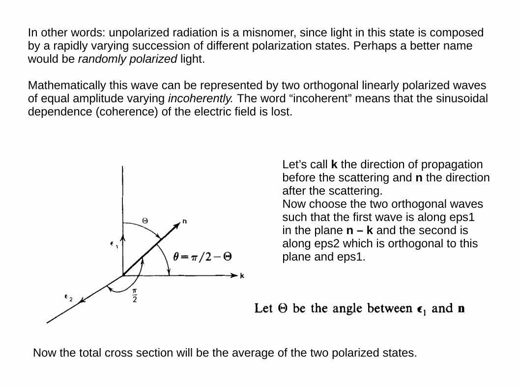
In other words: unpolarized radiation is a misnomer, since light in this state is composedby a rapidly varying succession of different polarization states. Perhaps a better namewould be randomly polarized light.

Mathematically this wave can be represented by two orthogonal linearly polarized wavesof equal amplitude varying incoherently. The word “incoherent” means that the sinusoidaldependence (coherence) of the electric field is lost.

Let’s call k the direction of propagationbefore the scattering and n the directionafter the scattering. Now choose the two orthogonal wavessuch that the first wave is along eps1in the plane n – k and the second is along eps2 which is orthogonal to thisplane and eps1.

Now the total cross section will be the average of the two polarized states.

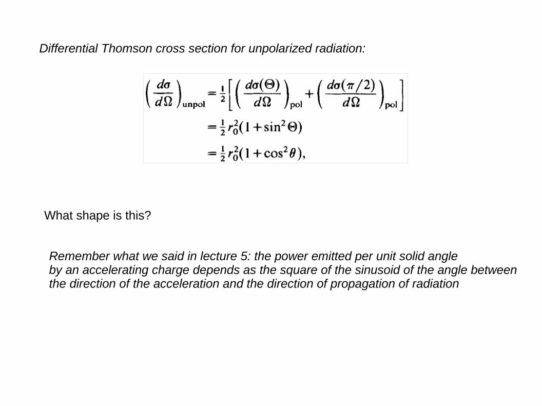
Differential Thomson cross section for unpolarized radiation:

What shape is this?

Remember what we said in lecture 5: the power emitted per unit solid angle by an accelerating charge depends as the square of the sinusoid of the angle betweenthe direction of the acceleration and the direction of propagation of radiation

Larmor’s Formula

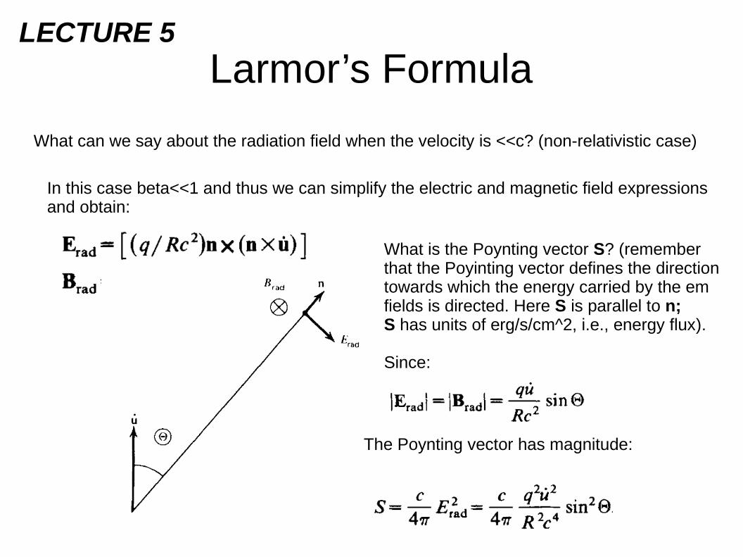
What can we say about the radiation field when the velocity is <<c? (non-relativistic case)

In this case beta<<1 and thus we can simplify the electric and magnetic field expressionsand obtain:

What is the Poynting vector S? (remember that the Poyinting vector defines the directiontowards which the energy carried by the em fields is directed. Here S is parallel to n; S has units of erg/s/cm^2, i.e., energy flux).

Since:

The Poynting vector has magnitude:

LECTURE 5

Larmor’s Formula

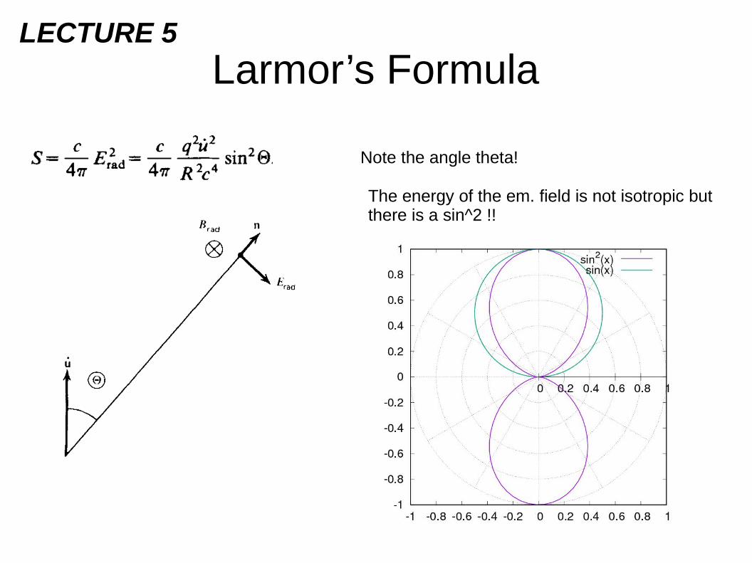
Note the angle theta!

The energy of the em. field is not isotropic butthere is a sin^2 !!

LECTURE 5

Larmor’s Formula

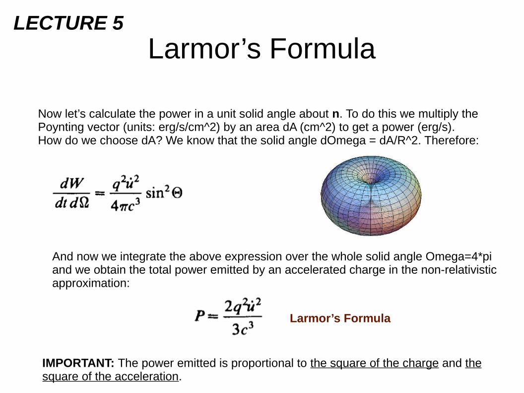
Now let’s calculate the power in a unit solid angle about n. To do this we multiply the Poynting vector (units: erg/s/cm^2) by an area dA (cm^2) to get a power (erg/s). How do we choose dA? We know that the solid angle dOmega = dA/R^2. Therefore:

And now we integrate the above expression over the whole solid angle Omega=4*piand we obtain the total power emitted by an accelerated charge in the non-relativisticapproximation:

Larmor’s Formula

IMPORTANT: The power emitted is proportional to the square of the charge and thesquare of the acceleration.

LECTURE 5

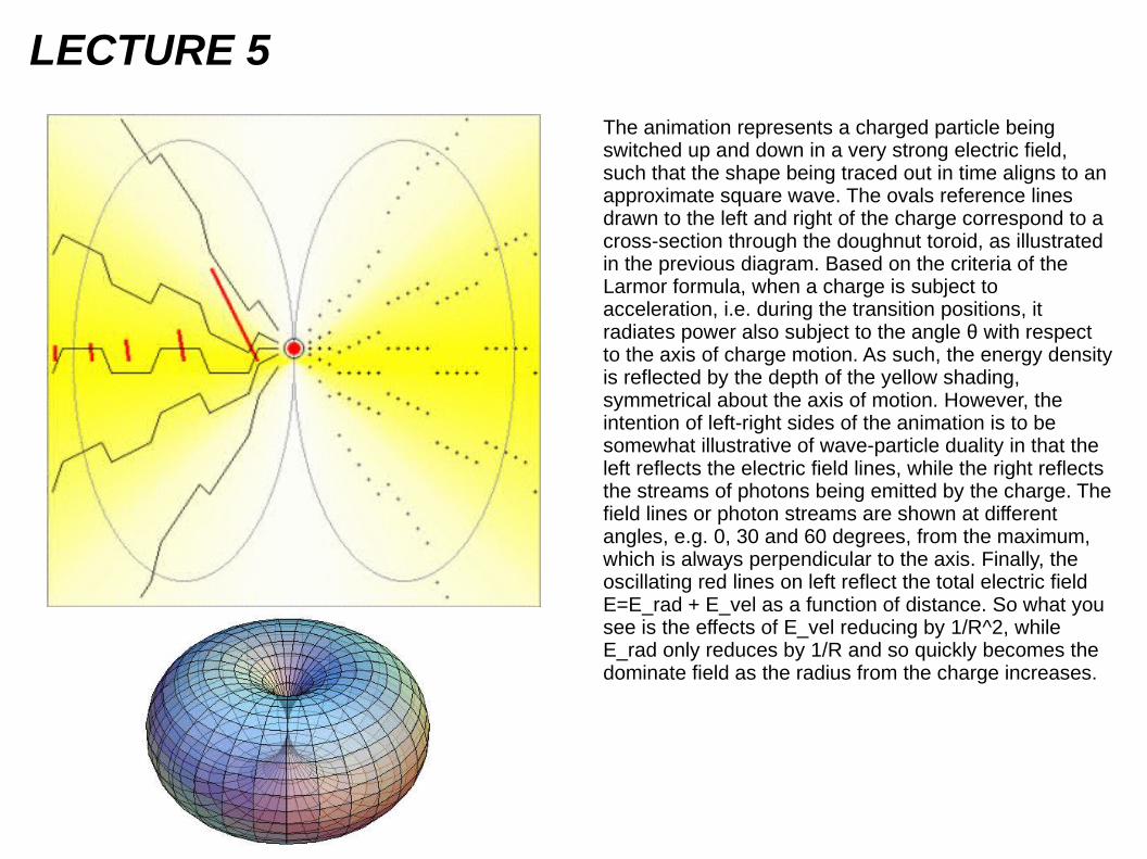
The animation represents a charged particle being switched up and down in a very strong electric field, such that the shape being traced out in time aligns to an approximate square wave. The ovals reference lines drawn to the left and right of the charge correspond to a cross-section through the doughnut toroid, as illustrated in the previous diagram. Based on the criteria of the Larmor formula, when a charge is subject to acceleration, i.e. during the transition positions, it radiates power also subject to the angle θ with respect to the axis of charge motion. As such, the energy density is reflected by the depth of the yellow shading, symmetrical about the axis of motion. However, the intention of left-right sides of the animation is to be somewhat illustrative of wave-particle duality in that the left reflects the electric field lines, while the right reflects the streams of photons being emitted by the charge. The field lines or photon streams are shown at different angles, e.g. 0, 30 and 60 degrees, from the maximum, which is always perpendicular to the axis. Finally, the oscillating red lines on left reflect the total electric field E=E_rad + E_vel as a function of distance. So what you see is the effects of E_vel reducing by 1/R^2, while E_rad only reduces by 1/R and so quickly becomes the dominate field as the radius from the charge increases.

LECTURE 5

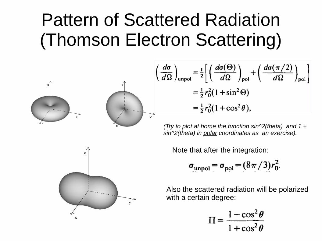
Pattern of Scattered Radiation (Thomson Electron Scattering)

(Try to plot at home the function sin^2(theta) and 1 + sin^2(theta) in polar coordinates as an exercise).

Note that after the integration:

Also the scattered radiation will be polarizedwith a certain degree:

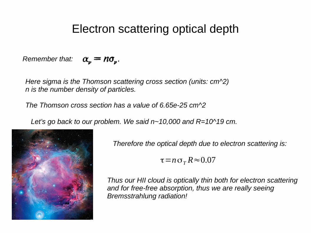
Electron scattering optical depth

Remember that:

Here sigma is the Thomson scattering cross section (units: cm^2)n is the number density of particles.

The Thomson cross section has a value of 6.65e-25 cm^2

Let’s go back to our problem. We said n~10,000 and R=10^19 cm.

Therefore the optical depth due to electron scattering is:

τ=nσT R≈0.07

Thus our HII cloud is optically thin both for electron scatteringand for free-free absorption, thus we are really seeing Bremsstrahlung radiation!

Covariance of E.M. Phenomena

So far we have not discussed the Relativistic Bremsstrahlung.

The reason is two-fold:

1. It is easier to understand it after we have explained the Compton scattering

2. We have not explained yet how electric and magnetic fields transform under Lorentz transformation.

We will see in Lecture 9 what Compton scattering is (and we will see that Thomson scattering is simply the low energy limit of the Compton scattering).

Now we will focus on the second point above, and use an intuitive approach to understand that the electrostatic field of an electron moving relativistically givesrise to a pulse of virtual radiation.

Covariance of Electromagnetic Phenomena

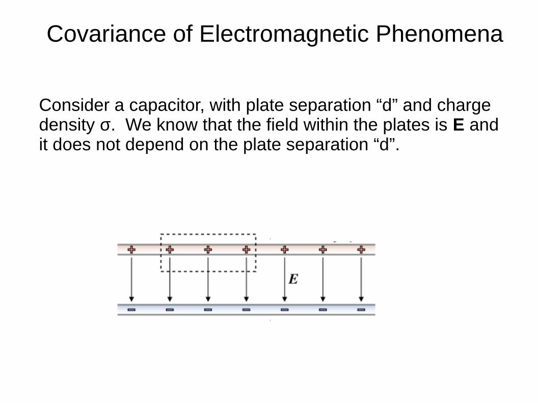
Consider a capacitor, with plate separation “d” and chargedensity σ. We know that the field within the plates is E and it does not depend on the plate separation “d”.

Covariance of Electromagnetic Phenomena

x

y

v

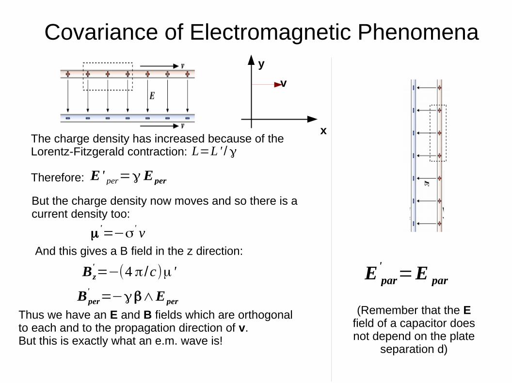
E par'

=E par

E ' per=γ Eper

(Remember that the E field of a capacitor does not depend on the plate

separation d)

Bper' =−γβ∧Eper

μ '=−σ ' v

The charge density has increased because of the Lorentz-Fitzgerald contraction:

Therefore:

L=L ' / γ

But the charge density now moves and so there is acurrent density too:

And this gives a B field in the z direction:

Bz'=−(4 π/c)μ '

Thus we have an E and B fields which are orthogonalto each and to the propagation direction of v. But this is exactly what an e.m. wave is!