Theoretical Surface ScienceWintersemester 2007/08

Axel Groß

Universitat Ulm, D-89069 Ulm, Germany

http://www.uni-ulm.de/theochem

Outline

1. Introduction

2. The Hamiltonian

3. Electronic Structure Methods and Total Energies

4. Approximate Interatomic Potentials

5. Dynamics of Processes on Surfaces

6. Kinetic Modelling of Processes on Surfaces

7. Electronically non-adiabatic Processes

8. Outlook

1. Introduction

Surfaces

• Processes on surfaces play an enormous-ly important technological role

• Harmful processes:

1. Rust, corrosion2. Wear

• Advantageous processes:

1. Production of chemicals2. Conversion of hazardous waste

Theoretical approach

• Some decades ago: phenomenologicalthermodynamic approach prevalent

• Nowadays: microscopic approach

• Theoretical surface science no longer li-mited to explanatory purposes

• Many surface processes can indeed bedescribed from first pricinples, i.e., with-out invoking any empirical parameter

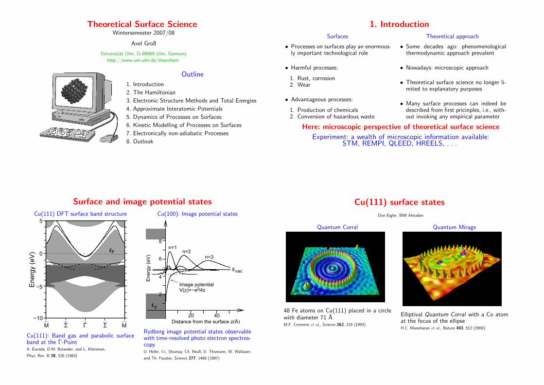
Here: microscopic perspective of theoretical surface science

Experiment: a wealth of microscopic information available:STM, REMPI, QLEED, HREELS, . . .

Surface and image potential states

Cu(111) DFT surface band structure

MΣ ΣΓ

εF

M

0

5

−10

−5Energ

y (e

V)

Cu(111): Band gas and parabolic surfaceband at the Γ-PointA. Euceda, D.M. Bylander, and L. Kleinman,

Phys. Rev. B 28, 528 (1983)

Cu(100): Image potential states

εF

20 40

2

Distance from the surface z(Å)

εvac

Image potentialV(z)=−e /4z

n=1n=2

n=3

Energ

y (e

V)

6

8

4

2

Rydberg image potential states observablewith time-resolved photo electron spectros-copyU. Hofer, I.L. Shumay, Ch. Reuß, U. Thomann, W. Wallauer,

and Th. Fauster, Science 277, 1480 (1997)

Cu(111) surface states

Don Eigler, IBM Almaden

Quantum Corral

48 Fe atoms on Cu(111) placed in a circlewith diameter 71 AM.F. Crommie et al., Science 262, 218 (1993).

Quantum Mirage

Elliptival Quantum Corral with a Co atomat the focus of the ellipseH.C. Manoharan et al., Nature 403, 512 (2000).

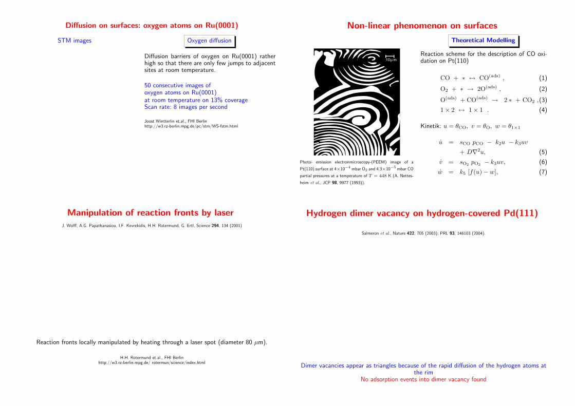
Diffusion on surfaces: oxygen atoms on Ru(0001)

STM images Oxygen diffusion

Diffusion barriers of oxygen on Ru(0001) ratherhigh so that there are only few jumps to adjacentsites at room temperature.

50 consecutive images ofoxygen atoms on Ru(0001)at room temperature on 13% coverageScan rate: 8 images per second

Joost Wintterlin et.al., FHI Berlinhttp://w3.rz-berlin.mpg.de/pc/stm/WS-fstm.html

Non-linear phenomenon on surfaces

µ10 m

Photo- emission electronmicroscopy-(PEEM) image of a

Pt(110) surface at 4×10−4 mbar O2 and 4.3×10−5 mbar CO

partial pressures at a temperature of T = 448 K (A. Nettes-

heim et al., JCP 98, 9977 (1993)).

Theoretical Modelling

Reaction scheme for the description of CO oxi-dation on Pt(110)

CO + ∗ ↔ CO(ads) , (1)

O2 + ∗ → 2O(ads) , (2)

O(ads) +CO(ads) → 2 ∗ + CO2 ,(3)

1× 2 ↔ 1× 1 . (4)

Kinetik: u = θCO, v = θO, w = θ1×1

u = sCO pCO − k2u − k3uv

+ D∇2u, (5)

v = sO2 pO2 − k3uv, (6)

w = k5 [f(u)− w], (7)

Manipulation of reaction fronts by laser

J. Wolff, A.G. Papathanasiou, I.F. Kevrekidis, H.H. Rotermund, G. Ertl, Science 294, 134 (2001)

Reaction fronts locally manipulated by heating through a laser spot (diameter 80 µm).

H.H. Rotermund et.al., FHI Berlinhttp://w3.rz-berlin.mpg.de/ rotermun/science/index.html

Hydrogen dimer vacancy on hydrogen-covered Pd(111)

Salmeron et al., Nature 422, 705 (2003); PRL 93, 146103 (2004).

Dimer vacancies appear as triangles because of the rapid diffusion of the hydrogen atoms atthe rim

No adsorption events into dimer vacancy found

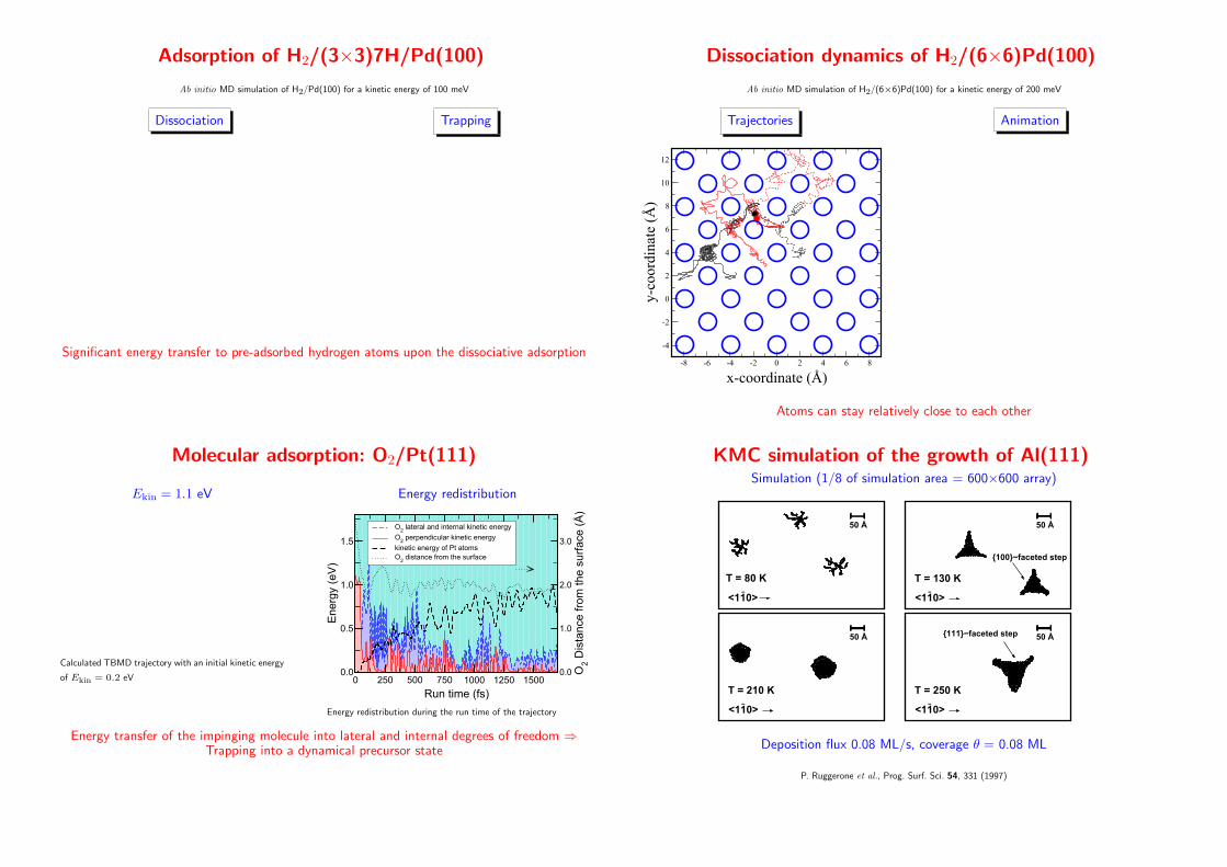
Adsorption of H2/(3×3)7H/Pd(100)

Ab initio MD simulation of H2/Pd(100) for a kinetic energy of 100 meV

Dissociation Trapping

Significant energy transfer to pre-adsorbed hydrogen atoms upon the dissociative adsorption

Dissociation dynamics of H2/(6×6)Pd(100)

Ab initio MD simulation of H2/(6×6)Pd(100) for a kinetic energy of 200 meV

Trajectories

-8 -6 -4 -2 0 2 4 6 8

x-coordinate (Å)

-4

-2

0

2

4

6

8

10

12

y-co

ordi

nate

(Å

)

Animation

Atoms can stay relatively close to each other

Molecular adsorption: O2/Pt(111)

Ekin = 1.1 eV

Calculated TBMD trajectory with an initial kinetic energy

of Ekin = 0.2 eV

Energy redistribution

0 250 500 750 1000 1250 1500

Run time (fs)

0.0

0.5

1.0

1.5

Energ

y (e

V)

O2 lateral and internal kinetic energy

O2 perpendicular kinetic energy

kinetic energy of Pt atomsO

2 distance from the surface

0.0

1.0

2.0

3.0

O2 D

ista

nce

fro

m t

he s

urf

ace

(Å

)

Energy redistribution during the run time of the trajectory

Energy transfer of the impinging molecule into lateral and internal degrees of freedom ⇒Trapping into a dynamical precursor state

KMC simulation of the growth of Al(111)Simulation (1/8 of simulation area = 600×600 array)

−<110>

T = 80 K

50 Å

−<110>

T = 130 K

50 Å

{100}−faceted step

−<110>

50 Å

T = 210 K−

<110>

50 Å

T = 250 K

{111}−faceted step

Deposition flux 0.08 ML/s, coverage θ = 0.08 ML

P. Ruggerone et al., Prog. Surf. Sci. 54, 331 (1997)

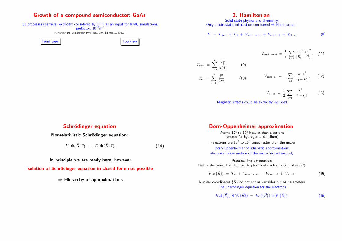
Growth of a compound semiconductor: GaAs

31 processes (barriers) explicitly considered by DFT as an input for KMC simulations,prefactor: 1013s−1

P. Kratzer and M. Scheffler, Phys. Rev. Lett. 88, 036102 (2002).

Front view Top view

2. HamiltonianSolid-state physics and chemistry:

Only electrostatic interaction considered ⇒ Hamiltonian:

H = Tnucl + Tel + Vnucl−nucl + Vnucl−el + Vel−el (8)

Tnucl =L∑

I=1

~P 2I

2MI, (9)

Tel =N∑

i=1

~p2i

2m, (10)

Vnucl−nucl =1

2

∑

I6=J

ZI ZJ e2

|~RI − ~RJ|, (11)

Vnucl−el = −∑

i,I

ZI e2

|~ri − ~RI|, (12)

Vel−el =1

2

∑

i 6=j

e2

|~ri − ~rj|. (13)

Magnetic effects could be explicitly included

Schrodinger equation

Nonrelativistic Schrodinger equation:

H Φ(~R,~r) = E Φ(~R,~r). (14)

In principle we are ready here, however

solution of Schrodinger equation in closed form not possible

⇒ Hierarchy of approximations

Born-Oppenheimer approximationAtoms 104 to 105 heavier than electrons

(except for hydrogen and helium)

⇒electrons are 102 to 103 times faster than the nuclei

Born-Oppenheimer of adiabatic approximation:

electrons follow motion of the nuclei instantaneously

Practical implementation:Define electronic Hamiltonian Hel for fixed nuclear coordinates {~R}

Hel({~R}) = Tel + Vnucl−nucl + Vnucl−el + Vel−el. (15)

Nuclear coordinates {~R} do not act as variables but as parameters

The Schrodinger equation for the electrons

Hel({~R}) Ψ(~r, {~R}) = Eel({~R}) Ψ(~r, {~R}). (16)

Born-Oppenheimer approximation II

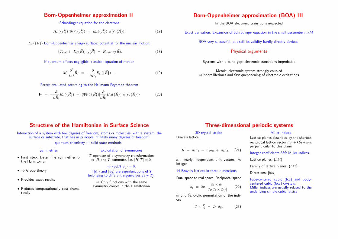
Schrodinger equation for the electrons

Hel({~R}) Ψ(~r, {~R}) = Eel({~R}) Ψ(~r, {~R}). (17)

Eel({~R}) Born-Oppenheimer energy surface: potential for the nuclear motion:

{Tnucl + Eel(~R)} χ(~R) = Enucl χ(~R). (18)

If quantum effects negligible: classical equation of motion

MI∂2

∂t2~RI = − ∂

∂ ~RIEel({~R}) . (19)

Forces evaluated according to the Hellmann-Feynman theorem

FI = − ∂

∂ ~RI

Eel({~R}) = 〈Ψ(~r, {~R})| ∂∂ ~RI

Hel({~R})|Ψ(~r, {~R})〉 (20)

Born-Oppenheimer approximation (BOA) III

In the BOA electronic transitions neglected

Exact derivation: Expansion of Schrodinger equation in the small parameter m/M

BOA very successful, but still its validity hardly directly obvious

Physical arguments

Systems with a band gap: electronic transitions improbable

Metals: electronic system strongly coupled⇒ short lifetimes and fast quenchening of electronic excitations

Structure of the Hamiltonian in Surface Science

Interaction of a system with few degrees of freedom, atoms or molecules, with a system, thesurface or substrate, that has in principle infinitely many degrees of freedom.

quantum chemistry ↔ solid-state methods.

Symmetries

• First step: Determine symmetries ofthe Hamiltonian

• ⇒ Group theory

• Provides exact results

• Reduces computationally cost drama-tically

Exploitation of symmetries

T operator of a symmetry transformation⇒ H and T commute, i.e. [H,T ] = 0.

⇒ 〈ψi|H|ψj〉 = 0,

if |ψi〉 and |ψj〉 are eigenfunctions of Tbelonging to different eigenvalues Ti 6= Tj.

⇒ Only functions with the samesymmetry couple in the Hamiltonian

Three-dimensional periodic systems

3D crystal latticeBravais lattice:

~R = n1~a1 + n2~a2 + n3~a3. (21)

ai linearly independent unit vectors, niinteger

14 Bravais lattices in three dimensions

Dual space to real space: Reciprocal space

~b1 = 2π~a2 × ~a3

|~a1(~a2 × ~a3)|(22)

~b2 and ~b3: cyclic permutation of the indi-ces

~ai · ~bj = 2π δij, (23)

Miller indices

Lattice planes described by the shortestreciprocal lattice vector h~b1+ k~b2+h~b3perpendicular to this plane

Integer coefficients hkl: Miller indices.

Lattice planes: (hkl)

Family of lattice planes: {hkl}Directions: [hkl]

Face-centered cubic (fcc) and body-centered cubic (bcc) crystals:Miller indices are usually related to theunderlying simple cubic lattice

Bloch Theorem

Bloch theorem illustrates power of group theory

HamiltonianConsider effective one-particle Schrodin-ger equation

{

− ~2

2m∇2 + veff(~r)

}

ψi(~r) = εiψi(~r).

(24)Effective one-particle potential veff(~r)satisfies translational symmetry:

veff(~r) = veff(~r + ~R), (25)

with ~R any Bravais lattice vector.

Exploitation of group theoryTranslations T~R form an Abelian group⇒ 1-D representation, eigenfunctions:

T~Rψi(~r) = ψi(~r + ~R) = ci(~R)ψi(~r) (26)

with ci(~R)ci(~R′) = ci(~R+ ~R′). (27)

⇒ ci(~R) = ei~k·~R. (28)

Eigenfunction ψi(~r) characterized by the

crystal-momentum ~k

ψ~k(~r) = ei~k·~r u~k(~r) (29)

with the periodic function

u~k(~r) = u~k(~r + ~R) (30)

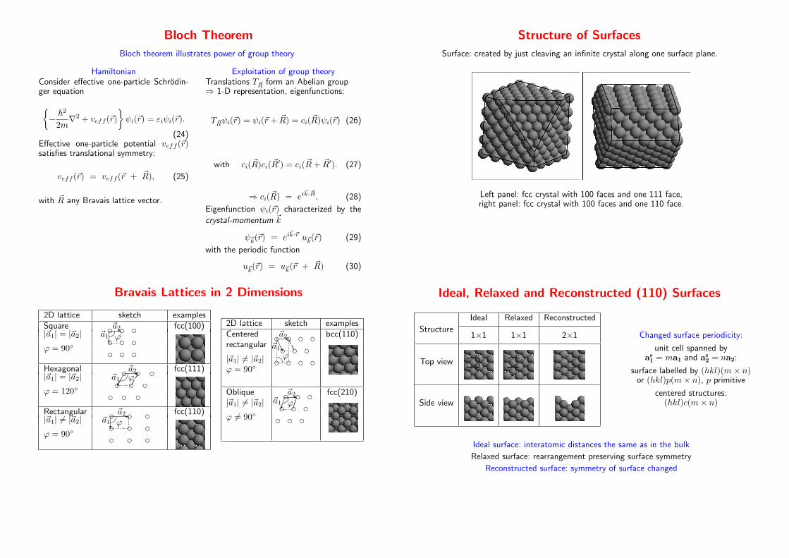
Structure of Surfaces

Surface: created by just cleaving an infinite crystal along one surface plane.

Left panel: fcc crystal with 100 faces and one 111 face,right panel: fcc crystal with 100 faces and one 110 face.

Bravais Lattices in 2 Dimensions

2D lattice sketch examplesSquare

hhh

hhh

hhh-

?�~a1

~a2

ϕfcc(100)

|~a1| = |~a2|ϕ = 90◦

Hexagonal h h hh h h

h h h

-������

�����

~a1

~a2ϕ

fcc(111)|~a1| = |~a2|ϕ = 120◦

Rectangular

hhh

hhh

hhh-

?�~a1

~a2

ϕfcc(110)

|~a1| 6= |~a2|ϕ = 90◦

2D lattice sketch examplesCentered

h h h hh h h

h h h h-AAAU�AAAA~a1

~a2

ϕ

bcc(110)rectangular

|~a1| 6= |~a2|ϕ = 90◦

Oblique

hh

h

hh

h

hh

h-���

�����

~a1

~a2

ϕfcc(210)

|~a1| 6= |~a2|ϕ 6= 90◦

Ideal, Relaxed and Reconstructed (110) Surfaces

Ideal Relaxed Reconstructed

Structure1×1 1×1 2×1

Top view

Side view

Changed surface periodicity:

unit cell spanned bya

s

1= ma1 and a

s

2= na2:

surface labelled by (hkl)(m× n)or (hkl)p(m× n), p primitive

centered structures:(hkl)c(m× n)

Ideal surface: interatomic distances the same as in the bulk

Relaxed surface: rearrangement preserving surface symmetry

Reconstructed surface: symmetry of surface changed

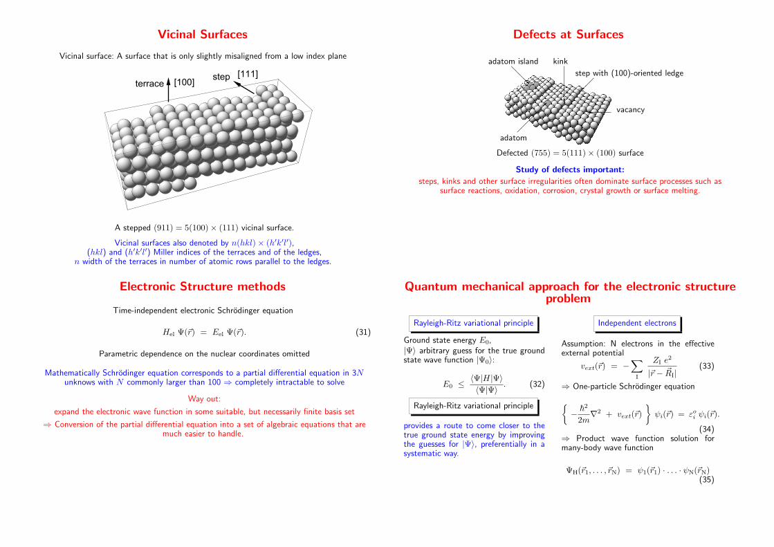
Vicinal Surfaces

Vicinal surface: A surface that is only slightly misaligned from a low index plane

[100]step

terrace[111]

A stepped (911) = 5(100)× (111) vicinal surface.

Vicinal surfaces also denoted by n(hkl)× (h′k′l′),(hkl) and (h′k′l′) Miller indices of the terraces and of the ledges,

n width of the terraces in number of atomic rows parallel to the ledges.

Defects at Surfaces

� vacancy

step with (100)-oriented ledge

?

kink@@@@@R

adatom island

�

adatom

Defected (755) = 5(111)× (100) surface

Study of defects important:

steps, kinks and other surface irregularities often dominate surface processes such assurface reactions, oxidation, corrosion, crystal growth or surface melting.

Electronic Structure methods

Time-independent electronic Schrodinger equation

Hel Ψ(~r) = Eel Ψ(~r). (31)

Parametric dependence on the nuclear coordinates omitted

Mathematically Schrodinger equation corresponds to a partial differential equation in 3Nunknows with N commonly larger than 100 ⇒ completely intractable to solve

Way out:

expand the electronic wave function in some suitable, but necessarily finite basis set

⇒ Conversion of the partial differential equation into a set of algebraic equations that aremuch easier to handle.

Quantum mechanical approach for the electronic structureproblem

Rayleigh-Ritz variational principle

Ground state energy E0,|Ψ〉 arbitrary guess for the true groundstate wave function |Ψ0〉:

E0 ≤〈Ψ|H|Ψ〉〈Ψ|Ψ〉 . (32)

Rayleigh-Ritz variational principle

provides a route to come closer to thetrue ground state energy by improvingthe guesses for |Ψ〉, preferentially in asystematic way.

Independent electrons

Assumption: N electrons in the effectiveexternal potential

vext(~r) = −∑

I

ZI e2

|~r − ~RI|(33)

⇒ One-particle Schrodinger equation

{

− ~2

2m∇2 + vext(~r)

}

ψi(~r) = εoi ψi(~r).

(34)⇒ Product wave function solution formany-body wave function

ΨH(~r1, . . . , ~rN) = ψ1(~r1) · . . . · ψN(~rN)(35)

Hartree Approximation I

Assume product wave function as a first guess for the many-body wave function

⇒ Expection value of the electronic Hamiltonian:

〈ΨH|H|ΨH〉 =N∑

i=1

∫

d~r ψ∗i (~r)

(

− ~2

2m∇2 + vext(~r)

)

ψi(~r)

+1

2

N∑

i,j=1

∫

d~rd~r′e2

|~r − ~r′| |ψi(~r)|2|ψj(~r′)|2 + Vnucl−nucl. (36)

Minimize the expectation value (36) with respect to more suitable single-particle functionsψi(~r) under the constraint that the wave functions are normalized:

δ

δψ∗k

[

〈ΨH|H|ΨH〉 −N∑

i=1

{εi(〈ψi|ψi〉 − 1)}]

= 0. (37)

εi: Lagrange multipliers ensuring the normalisation of the eigen functions.

Hartree Approximation II

Variation leads to the Hartree equations

− ~2

2m∇2 + vext(~r) +

N∑

j=1

∫

d~r′e2

|~r − ~r′| |ψj(~r′)|2

ψk(~r) = εk ψk(~r). (38)

Mean-field approximation: Hartree equations describe an electron embedded in theelectrostatic field of all electrons including the particular electron itself.

This causes the self interaction which is erroneously contained in the Hartree equations.

Define electron density n(~r) and Hartree potential vH:

n(~r) =N∑

i=1

|ψi(~r)|2, vH(~r) =

∫

d~r′ n(~r′)e2

|~r − ~r′| (39)

⇒ Hartree equations:{

− ~2

2m∇2 + vext(~r) + vH(~r)

}

ψi(~r) = εi ψi(~r). (40)

Hartree Approximation III

Hartree equations:{

− ~2

2m∇2 + vext(~r) + vH(~r)

}

ψi(~r) = εi ψi(~r). (41)

Solutions ψi(~r) of the Hartree equations enter the effective one-particle Hamiltionan:

⇒ Hartree equations can only be solved in an iterative fashion

⇒ Hartree approximation ≡ “self-consistent field approximation”.

Expectation value of the total energy in the Hartree approximation EH:

〈ΨH|H|ΨH〉 =N∑

i=1

εi −1

2

∫

d~r d~r′e2 n(~r) n(~r′)

|~r − ~r′| + Vnucl−nucl

=N∑

i=1

εi − VH + Vnucl−nucl = EH (42)

Hartree energy VH enters the Hartree eigenvalues twice ⇒ has to be subtracted.Reflects the interaction between particles in a self-consistent scheme.

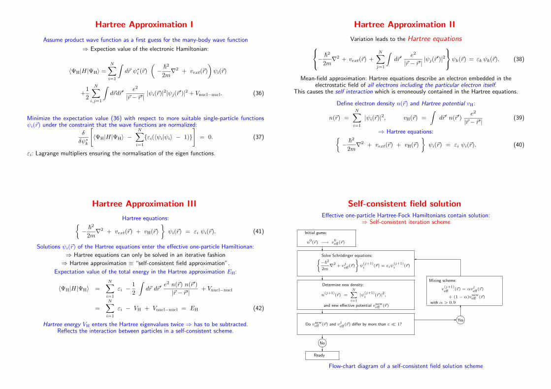
Self-consistent field solutionEffective one-particle Hartree-Fock Hamiltonians contain solution:

⇒ Self-consistent iteration scheme

Initial guess:

n0(~r) −→ v

0eff(~r)

?

Solve Schrodinger equations:(

−~2

2m∇2

+ vjeff

(~r)

)

ψ(j+1)i (~r) = εiψ

(j+1)i (~r)

?

Determine new density:

n(j+1)

(~r) =

NX

i=1

|ψ(j+1)i (~r)|2,

and new effective potential vneweff (~r)

?

Do vneweff (~r) and v

jeff

(~r) differ by more than ε≪ 1?

?

����No

?

Ready

-����Yes

6

Mixing scheme:

v(j+1)eff

(~r) = αvjeff

(~r)

+ (1− α)vneweff (~r)

with α > 0.9

�

Flow-chart diagram of a self-consistent field solution scheme

Hartree-Fock Approximation I

Hartree ansatz only partially obeys the Pauli principleby populating each electronic state once,

but it does not take into account the anti-symmetry of the wave function.

⇒ Construction of a Slater determinant from the single-particle functions ψ(~rσ),where σ denotes the spin:

ΨHF(~r1σ1, . . . , ~rNσN) =1√N !

∣

∣

∣

∣

∣

∣

∣

∣

ψ1(~r1σ1) ψ1(~r2σ2) . . . ψ1(~rNσN)ψ2(~r1σ1) ψ2(~r2σ2) . . . ψ2(~rNσN)

... ... . . . ...ψN(~r1σ1) ψN(~r2σ2) . . . ψN(~rNσN)

∣

∣

∣

∣

∣

∣

∣

∣

. (43)

Hartree-Fock Approximation II

Follow same procedure as in the Hartree ansatz: first write down expectation value

〈ΨHF|H|ΨHF〉 =N∑

i=1

∫

d~r ψ∗i (~r)

(

− ~2

2m∇2 + vext(~r)

)

ψi(~r)

+1

2

N∑

i,j=1

∫

d~r d~r′e2

|~r − ~r′| |ψi(~r)|2 |ψj(~r′)|2

−12

N∑

i,j=1

∫

d~rd~r′e2

|~r − ~r′| δσiσjψ∗i (~r)ψi(~r

′)ψ∗j (~r′)ψj(~r).

+ Vnucl−nucl . (44)

σi spin of the state ψi(~r)

Hartree-Fock Approximation III

Minimize expectation value of total energy with respect to the ψ∗i under the constraint ofnormalization:

{

− ~2

2m∇2 + vext(~r) + vH(~r)

}

ψi(~r)

−N∑

j=1

∫

d~r′e2

|~r − ~r′| ψ∗j (~r

′)ψi(~r′)ψj(~r)δσiσj

= εi ψi(~r). (45)

Additional term, exchange term, integral operator:∫

V (~r, ~r′)ψ(~r′)d~r′

Total energy in the Hartree-Fock approximation:

〈ΨHF|H|ΨHF〉 = EHF =N∑

i=1

εi − VH − Ex + Vnucl−nucl (46)

Homogeneous electron gas

Homogeneous electron gas: n(~r) uniform.

Assumption: electrostatic potential of the electronscompensated by a positive charge background.

⇒ “jellium model”:

vext(~r) + vH(~r) = 0 . (47)

Eigenfunctions of the Hartree equations for the homogeneous electron gas(periodic boundary conditions):

ψi(~r) =1√Vei~ki·~r. (48)

Plane waves

Exchange in the homogeneous electron gas

Total energy: Hartree term VH exactly cancels with Vnucl−nucl

EH =N∑

i=1

ε(~ki) = 2∑

|~k|<kF

~2~k2

2m. (49)

Fermi vector kF: vector of the occupied one-electron levels of highest energy,

kF =

(

3π2N

V

)1/3

=(

3π2n)1/3

(50)

Hartree-Fock: plane waves are still eigenfunctions for the homogeneous electron gas

ε(~k) =~

2~k2

2m− 2e2

πkF F

(

k

kF

)

(51)

F (x) =1

2+

1 − x2

4xln

∣

∣

∣

∣

1 + x

1 − x

∣

∣

∣

∣

. (52)

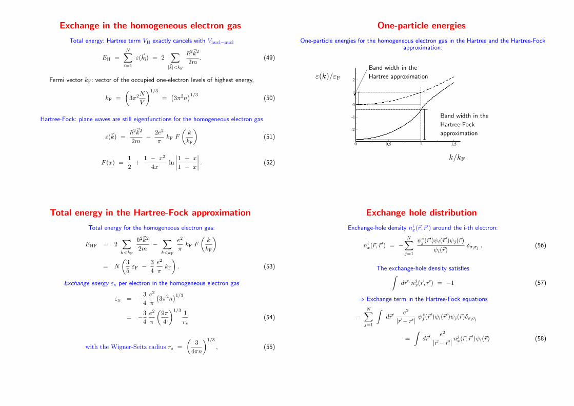
One-particle energies

One-particle energies for the homogeneous electron gas in the Hartree and the Hartree-Fockapproximation:

0 0,5 1 1,5

-2

-1

0

1

2ε(k)/εF

k/kF

Band width in the

Hartree-Fock

approximation

����������

Band width in the

Hartree approximation

Total energy in the Hartree-Fock approximation

Total energy for the homogeneous electron gas:

EHF = 2∑

k<kF

~2~k2

2m−

∑

k<kF

e2

πkF F

(

k

kF

)

= N

(

3

5εF − 3

4

e2

πkF

)

. (53)

Exchange energy εx per electron in the homogeneous electron gas

εx = −34

e2

π

(

3π2n)1/3

= −34

e2

π

(

9π

4

)1/31

rs(54)

with the Wigner-Seitz radius rs =

(

3

4πn

)1/3

, (55)

Exchange hole distribution

Exchange-hole density nix(~r, ~r′) around the i-th electron:

nix(~r, ~r′) = −

N∑

j=1

ψ∗j (~r′)ψi(~r′)ψj(~r)

ψi(~r)δσiσj

. (56)

The exchange-hole density satisfies∫

d~r′ njx(~r, ~r′) = −1 (57)

⇒ Exchange term in the Hartree-Fock equations

−N∑

j=1

∫

d~r′e2

|~r − ~r′| ψ∗j (~r

′)ψi(~r′)ψj(~r)δσiσj

=

∫

d~r′e2

|~r − ~r′| njx(~r, ~r

′)ψi(~r) (58)

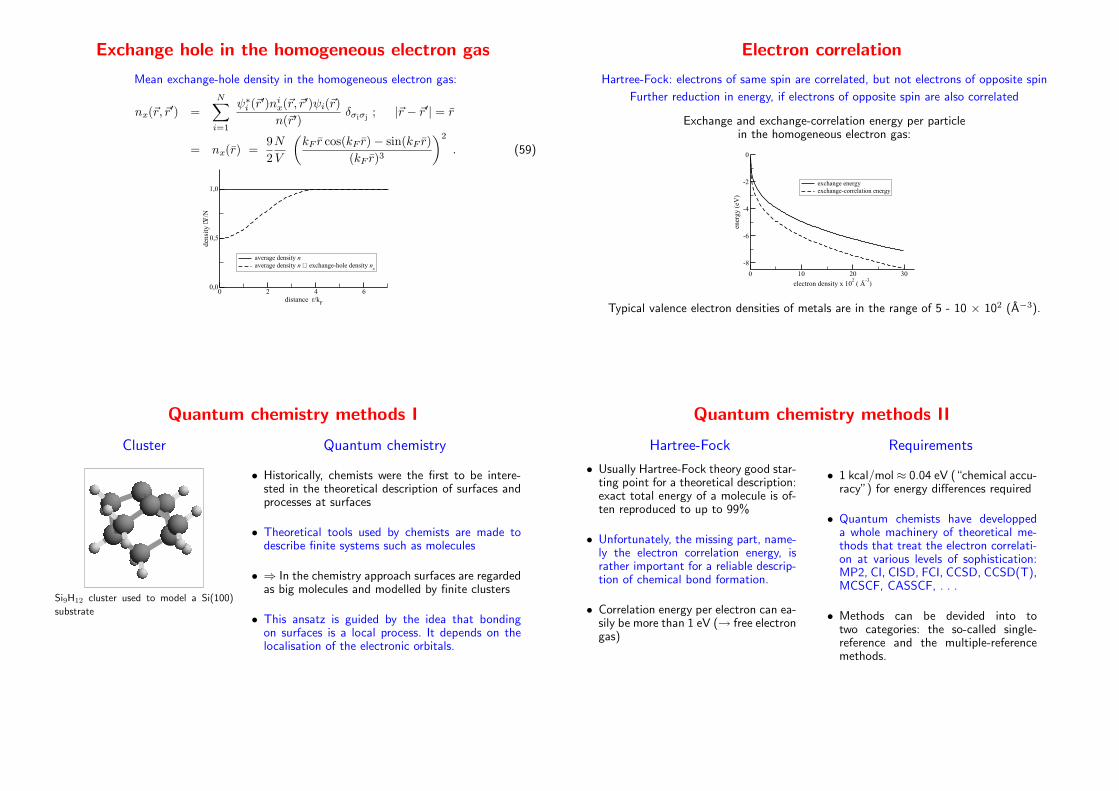
Exchange hole in the homogeneous electron gas

Mean exchange-hole density in the homogeneous electron gas:

nx(~r, ~r′) =

N∑

i=1

ψ∗i (~r′)nix(~r, ~r

′)ψi(~r)

n(~r′)δσiσj

; |~r − ~r′| = r

= nx(r) =9

2

N

V

(

kF r cos(kF r)− sin(kF r)

(kF r)3

)2

. (59)

0 2 4 6distance r/k

F

0,0

0,5

1,0

dens

ity

⋅V/N

average density naverage density n + exchange-hole density n

x

Electron correlation

Hartree-Fock: electrons of same spin are correlated, but not electrons of opposite spin

Further reduction in energy, if electrons of opposite spin are also correlated

Exchange and exchange-correlation energy per particlein the homogeneous electron gas:

0 10 20 30

electron density x 102 ( Å

-3)

-8

-6

-4

-2

0

ener

gy (

eV)

exchange energyexchange-correlation energy

Typical valence electron densities of metals are in the range of 5 - 10 × 102 (A−3).

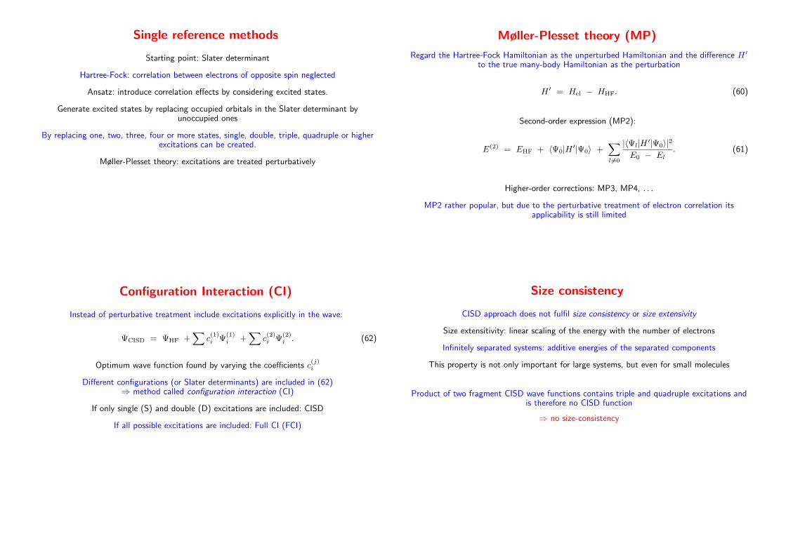
Quantum chemistry methods I

Cluster

Si9H12 cluster used to model a Si(100)

substrate

Quantum chemistry

• Historically, chemists were the first to be intere-sted in the theoretical description of surfaces andprocesses at surfaces

• Theoretical tools used by chemists are made todescribe finite systems such as molecules

• ⇒ In the chemistry approach surfaces are regardedas big molecules and modelled by finite clusters

• This ansatz is guided by the idea that bondingon surfaces is a local process. It depends on thelocalisation of the electronic orbitals.

Quantum chemistry methods II

Hartree-Fock

• Usually Hartree-Fock theory good star-ting point for a theoretical description:exact total energy of a molecule is of-ten reproduced to up to 99%

• Unfortunately, the missing part, name-ly the electron correlation energy, israther important for a reliable descrip-tion of chemical bond formation.

• Correlation energy per electron can ea-sily be more than 1 eV (→ free electrongas)

Requirements

• 1 kcal/mol ≈ 0.04 eV (“chemical accu-racy”) for energy differences required

• Quantum chemists have developpeda whole machinery of theoretical me-thods that treat the electron correlati-on at various levels of sophistication:MP2, CI, CISD, FCI, CCSD, CCSD(T),MCSCF, CASSCF, . . .

• Methods can be devided into totwo categories: the so-called single-reference and the multiple-referencemethods.

Single reference methods

Starting point: Slater determinant

Hartree-Fock: correlation between electrons of opposite spin neglected

Ansatz: introduce correlation effects by considering excited states.

Generate excited states by replacing occupied orbitals in the Slater determinant byunoccupied ones

By replacing one, two, three, four or more states, single, double, triple, quadruple or higherexcitations can be created.

Møller-Plesset theory: excitations are treated perturbatively

Møller-Plesset theory (MP)

Regard the Hartree-Fock Hamiltonian as the unperturbed Hamiltonian and the difference H ′

to the true many-body Hamiltonian as the perturbation

H ′ = Hel − HHF. (60)

Second-order expression (MP2):

E(2) = EHF + 〈Ψ0|H ′|Ψ0〉 +∑

l 6=0

|〈Ψl|H ′|Ψ0〉|2E0 − El

. (61)

Higher-order corrections: MP3, MP4, . . .

MP2 rather popular, but due to the perturbative treatment of electron correlation itsapplicability is still limited

Configuration Interaction (CI)

Instead of perturbative treatment include excitations explicitly in the wave:

ΨCISD = ΨHF +∑

c(1)i Ψ

(1)i +

∑

c(2)i Ψ

(2)i . (62)

Optimum wave function found by varying the coefficients c(j)i

Different configurations (or Slater determinants) are included in (62)⇒ method called configuration interaction (CI)

If only single (S) and double (D) excitations are included: CISD

If all possible excitations are included: Full CI (FCI)

Size consistency

CISD approach does not fulfil size consistency or size extensivity

Size extensitivity: linear scaling of the energy with the number of electrons

Infinitely separated systems: additive energies of the separated components

This property is not only important for large systems, but even for small molecules

Product of two fragment CISD wave functions contains triple and quadruple excitations andis therefore no CISD function

⇒ no size-consistency

Coupled Cluster Theory (CC)

Recover size extensitivity by exponentiating single and double excitations operator:

ΨCCSD = exp(T1 + T2) ΨHF. (63)

Coupled cluster (CC) theory

Limitation to single and double excitations: CCSD

Triple excitations included: CCSDT

CCSDT has an eight-power dependence on the size of the system

Perturbative treatment of triple excitations: CCSD(T)

CCSD(T) calculations are method of choice for very accurate determination of molecularequilibrium structures

Multiple reference methods

Single-reference methods very reliable in the vicinity of equilibrium configurations

Often they are not adequate to describe a bond-breaking process:

Dissociation products should be described by a linear combination of two Slater determinantstaking into account the proper spin state

⇒ One Slater determinant plus excited states derived from this determinant not sufficient

Accuracy can be systematically improved by considering more and more configurations⇒ Full configuration interaction (FCI)

Because of the large required computational effort, FCI calculations are limited to rathersmall systems.

Approximate multi-reference methods are needed

SCF methods

Multiconfigurational self-consistent field (MCSCF) approach:

A relatively small number of configurations selected and both the orbitals and theconfiguration interactions coefficients are determined variationally

⇒ Chemical insight needed for the selection of the configurations

Complete active space (CASSCF) approach:

A set of active orbitals identified and all excitations within this active space are included.

Method computationally very costly

Basis set nomenclature

Preferred basis set in quantum chemistry: Gaussian functions⇒ integral can be evaluated analytically

Nomenclature:

One atomic orbital per valence state: “minimal basis set” or “single zeta”

Two or more orbitals: “double zeta”(DZ), “triple zeta” (TZ) and so on

Often polarization functions added (one or more sets of d functions on first row atoms): “P”added to the acronym of the basis, e.g., DZ2P

Delocalized states (anionic or Rydberg excited states): further diffuse functions added

Density functional theory (DFT)

Wave function based methods limited to a small number of atoms due to unfavorable scaling

Electronic structure methods based on density more efficient: DFT

DFT based upon the Hohenberg-Kohn theorem:

The ground-state density n(~r) of a system of interacting electrons in an external potentialuniquely determines this potential

Proof simple!

Density n(~r) uniquely related to the external potential and the number N of electrons viaN =

∫

n(~r)d~r

⇒ n(~r) determines the full Hamiltonian

In principle it determines all quantities that can be derived from the Hamiltonian such as,e.g., the electronic excitation spectrum

Unfortunately this has no practical consequences since the dependence is only implicit

Variational principle

Variational principle for the energy functional:

Etot = minn(~r)

E[n] = minn(~r)

(T [n] + Vext[n] + VH[n] + Exc[n]). (64)

Vext[n] functional of the external potentialU [n] functional of the classical electrostatic interaction energy (Hartree energy)

T [n] is the kinetic energy functional for non-interacting electrons

All quantum mechanical many-body effects are contained in the so-calledexchange-correlation functional Exc[n]

This non-local functional is not known in general

Important property: Exc[n] universal functional of the electron density

Advantage: Instead of using the many-body quantum wave function which depends on 3Ncoordinates now only a function of three coordinates has to be varied.

Kohn-Sham equations

In practice no direct variation of the density is performed because, e.g., the kinetic energyfunctional T [n] is not well-known

Express density as a sum over single-particle states

n(~r) =

N∑

i=1

|ψi(~r)|2, (65)

Minimize E[n] with respect to the single particle states under the constraint ofnormalization: ⇒ Kohn-Sham equations

{

− ~2

2m∇2 + vext(~r) + vH(~r) + vxc(~r)

}

ψi(~r) = εi ψi(~r) . (66)

Exchange-correlation potential vxc(~r):

vxc(~r) =δExc[n]

δn. (67)

Again: “single-particle energies”εi enter the formalism just as Lagrange multipliers.

Ground state energy in DFT

Ground state energy

E =N∑

i=1

εi + Exc[n] −∫

vxc(~r)n(~r) d~r − VH (68)

If the exchange-correlation terms Exc and vxc are neglected ⇒ Hartree approximation

Difference to Hartree and the Hartree-Fock approximation:

Ground-state energy (102) is in principle exact

Reliability of any practical implementation of DFT depends crucially on the accuracy of theexpression for the exchange-correlation functional

Exchange-correlation functional

Exchange-correlation functional Exc[n]:

Exc[n] =

∫

d~r n(~r) εxc[n](~r), (69)

Introduce exchange-correlation hole distribution

nxc(~r, ~r′) = g(~r, ~r′) − n(~r′) , (70)

g(~r, ~r′) conditional density to find an electron at ~r′ if there is already an electron at ~r

Sum rules:∫

d~r′ nxc(~r, ~r′) = −1 (71)

nxc(~r, ~r′) −→|~r−~r′|→∞

0 . (72)

∫

d~r′nxc(~r, ~r

′)

|~r − ~r′| −→|~r|→∞

− 1

|~r| (73)

Local Density Approximation (LDA)

Exchange-correlation energy per particle εxc[n](~r) not known in general

Local density approximation: use exchange-correlation energy for the homogeneous electrongas also for non-homogeneous situations

ELDAxc [n] =

∫

d3~r n(~r) εLDAxc (n(~r)) (74)

In a wide range of bulk and surface problems LDA surprisingly successful

Reasons still not fully understood, probably:

Cancellation of opposing errors in the LDA exchange and correlation

LDA satisfies the sum rules

For chemical reactions in the gas phase and at surfaces, however, the LDA results are notsufficiently accurate.

Usually LDA shows over-binding, i.e. binding and cohesive energies are too large and latticeconstants and bond lengths are too small

Generalized Gradient Approximation (GGA)

Straightforward Taylor expansion of the exchange-correlation energy εxc[n]:

Sum rules violated

Generalized gradient approximation: modify dependence on the gradient in such a way as tosatisfy sum rules

EGGAxc [n] =

∫

d3~r n(~r) εGGAxc (n(~r), |∇n(~r|) , (75)

DFT calculations in the GGA achieve chemical accuracy (error ≤ 0.1 eV) for many chemicalreactions; Example:

Dissociation barrier for H2/Cu(111)

LDA: 0.05 eV PW91-GGA: 0.6 eV Exp.: 0.5 - 0.7 eV

Problematic systems within the GGA

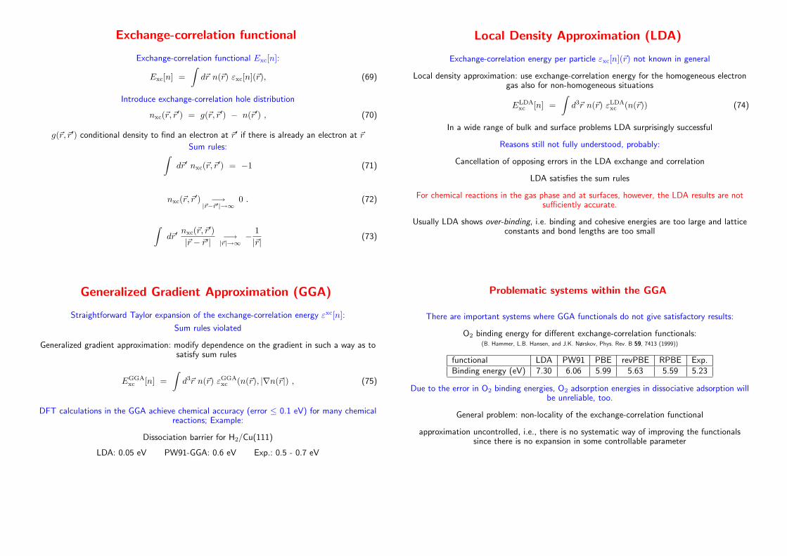
There are important systems where GGA functionals do not give satisfactory results:

O2 binding energy for different exchange-correlation functionals:(B. Hammer, L.B. Hansen, and J.K. Nørskov, Phys. Rev. B 59, 7413 (1999))

functional LDA PW91 PBE revPBE RPBE Exp.Binding energy (eV) 7.30 6.06 5.99 5.63 5.59 5.23

Due to the error in O2 binding energies, O2 adsorption energies in dissociative adsorption willbe unreliable, too.

General problem: non-locality of the exchange-correlation functional

approximation uncontrolled, i.e., there is no systematic way of improving the functionalssince there is no expansion in some controllable parameter

Pseudopotential

Chemical properties of most atoms are determined by their valence electrons.⇒ Pseudopotentials

Schrodinger equation with pseudopotential

{

− ~2

2m∇2 + vps

}

| ψps 〉 = εv | ψps 〉 . (76)

with

vps = veff(~r) +∑

i

(εv − εci) |ψci〉 〈ψci| . (77)

vps non-local and energy-dependent

|ψps〉 is not normalized

Norm-conserving pseudopotentials

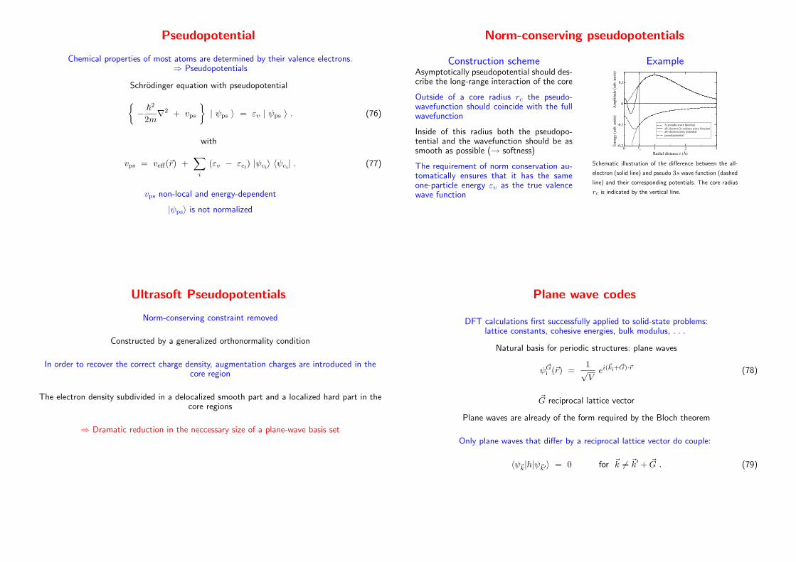
Construction schemeAsymptotically pseudopotential should des-cribe the long-range interaction of the core

Outside of a core radius rc the pseudo-wavefunction should coincide with the fullwavefunction

Inside of this radius both the pseudopo-tential and the wavefunction should be assmooth as possible (→ softness)

The requirement of norm conservation au-tomatically ensures that it has the sameone-particle energy εv as the true valencewave function

Example

0 rc 1 2 3

Radial distance r (Å)

-0,2

-0,1

0

0,1

Ene

rgy

(arb

. uni

ts)

Am

plit

ude

(arb

. uni

ts)

3s pseudo-wave functionall-electron 3s valence wave functionall-electron ionic potentialpseudopotential

Schematic illustration of the difference between the all-

electron (solid line) and pseudo 3s wave function (dashed

line) and their corresponding potentials. The core radius

rc is indicated by the vertical line.

Ultrasoft Pseudopotentials

Norm-conserving constraint removed

Constructed by a generalized orthonormality condition

In order to recover the correct charge density, augmentation charges are introduced in thecore region

The electron density subdivided in a delocalized smooth part and a localized hard part in thecore regions

⇒ Dramatic reduction in the neccessary size of a plane-wave basis set

Plane wave codes

DFT calculations first successfully applied to solid-state problems:lattice constants, cohesive energies, bulk modulus, . . .

Natural basis for periodic structures: plane waves

ψ~Gi (~r) =

1√Vei(~ki+~G)·~r (78)

~G reciprocal lattice vector

Plane waves are already of the form required by the Bloch theorem

Only plane waves that differ by a reciprocal lattice vector do couple:

〈ψ~k|h|ψ~k′〉 = 0 for ~k 6= ~k′ + ~G . (79)

Plane wave codes II

For periodic, infinite systems, the band structure energy in the total energy expression has tobe replaced by an integral over the first Brillouin zone:

∑

i

εi −→∑

bands

V

(2π)3

∫

BZ

d~k ε(~k) (80)

Integral can be approximated rather accurately by a sum over a finite set of ~k-points, eitherby using equally spaced ~k-points or so-called special ~k-points

Parameter characterizing the size of the plane wave basis: cutoff energy

Ecutoff = max~G

~2(~k + ~G)2

2m(81)

Norm-conserving Troullier-Martins pseudopotentials:cutoff energy ∼10 Ryd for semiconductors and ≥50 Ry for transition metals

Ultrasoft pseudopotentials: cutoff energy for transition metals reduced to about 20 Ryd ≈250 eV.

Plane wave codes for surface problems

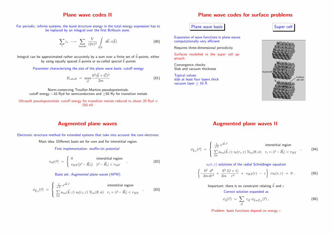
Plane wave basis

Expansion of wave functions in plane wavescomputationally very efficient

Requires three-dimensional periodicity

Surfaces modelled in the super cell ap-proach

Convergence checks:Slab and vacuum thickness

Typical values:slab at least four layers thickvacuum layer ≥ 10 A

Super cell

Augmented plane waves

Electronic structure method for extended systems that take into account the core electrons:

Main idea: Different basis set for core and for interstitial region.

First implementation: muffin-tin potential

veff(~r) =

{

0 interstitial region

vMT(|~r − ~Ri|) |~r − ~Ri| < rMT

, (82)

Basis set: Augmented plane waves (APW)

φ~k,ε(~r) =

1√Vei~k·~r interstitial region

∑

lm

alm(~k, ε) ul(ri, ε) Ylm(θ, φ) ri = |~r − ~Ri| < rMT, (83)

Augmented plane waves II

φ~k,ε(~r) =

1√Vei~k·~r interstitial region

∑

lm

alm(~k, ε) ul(ri, ε) Ylm(θ, φ) ri = |~r − ~Ri| < rMT, (84)

ul(r, ε) solutions of the radial Schrodinger equation{

− ~2

2m

d2

dr2+

~2

2m

l(l + 1)

r2+ vMT(r) − ε

}

rul(r, ε) = 0 . (85)

Important: there is no constraint relating ~k and ε

Correct solution expanded as

ψ~k(~r) =∑

~G

c~G φ~k+~G,ε(~r) , (86)

Problem: basis functions depend on energy ε

Linearized augmented plane waves

Problem of energy-depended basis functions avoided by the concept of linearized augmentedplane waves (LAPW): O.K. Andersen (1975)

Idea: expand radial function around fixed energy εl:

ul(r, ε) = ul(r, εl) + ul(r, εl) (ε− εl) + . . . , (87)

ul(r, εl) energy derivative

ul(r, εl) =dul(r, ε)

dε

∣

∣

∣

∣

ε=εl

. (88)

εl should be in the middle of the corresponding energy band with l character.

Linearized augmented plane waves II

LAPW basis functions:

φ~k(~r) =

1√Vei~k·~r interstitial region

∑

lm

[

alm(~k) ul(ri, εl) +

blm(~k) ul(ri, εl)]

Ylm(θ, φ) |~r − ~Ri| < rMT

(89)

alm(~k) and blm(~k) determined through the continuity requirement of both the wave functionand its first derivative.

FP-LAPW: no restriction to spherical symmetric potentials in the core region

veff(~r) =

∑

~G

veff(~G) ei ~G·~r interstitial region

∑

lm

vlmeff (ri) Ylm(θ, φ) |~r − ~Ri| < rMT

. (90)

Tight-Binding

Ab initio electronic structure methods still computationally expensive

There is a need for a approximative method that retains the quantum nature of bonding:Tight-binding

Tight-binding: expansion of the eigenstates of the effective one-particle Hamiltonian in anatomic-like basis set and replacing the exact many-body Hamiltonian with parametrized

Hamiltonian matrix elements

Formally, one starts with a basis of atomic functions

φiα(~r) = φα(~r − ~Ri) , (91)

i lattice site, α type of the atomic orbital

Periodic functions constructed by forming Bloch sums

φα~k(~r) =1√N

∑

i

ei~k·~Ri φα(~r − ~Ri) , (92)

Tight-Binding II

Bloch sums are used to determine Hamiltonian matrix elements:

hαβ(~k) = 〈φα~k|h|φβ~k〉

=∑

j

ei~k·~Rj 〈φ0α|h|φjβ〉 =

∑

j

ei~k·~Rj hαβ(~Rj) . (93)

Two-center approximation for hαβ(~Rj):

hαβ(~R) function of R = |~R| and of the direction cosines k, l,m of ~R.

Eigenfunctions χ~k of the one-particle Hamiltonian

χ~k(~r) =∑

α

cα(~k) φα~k(~r) . (94)

Nonorthogonal tight-binding

Eigenfunctions χ~k of the one-particle Hamiltonian

χ~k(~r) =∑

α

cα(~k) φα~k(~r) . (95)

Energies determined by eigenvalue equation

h(~k) c(~k) = S(~k) ε(~k) c(~k), (96)

S(~k) overlap matrix

Sαβ(~k) =∑

j

ei~k·~Rj 〈φ0α|φjβ〉 =

∑

j

ei~k·~Rj Sαβ(~Rj) . (97)

⇒ Dispersion curves ε(~k) obtained by the diagonalization of S(~k)−1h(~k).Nonorthogonal tight-binding

Orthogonal tight-binding

Further simplification: Assume that the atomic orbitals are already orthogonalized accordingto the Lowdin scheme

ψiα(~r) =∑

jβ

S−1/2iαjβ φjβ(~r) , (98)

⇒ Dispersion curves ε(~k) obtained by the diagonalization of h(~k).

Nc atoms in the unit cell and l atomic orbitals per atoms⇒ Ncl ×Ncl matrix has to be diagonalized

Atomic basis function do not explicitly appear in tight-binding⇒ parametrization scheme determines the reliability and accuracy of any tight-binding

calculation

Total energies in tight-binding

Total energies: usually a repulsive term written as a sum of pair terms is added to the bandenergy (can be derived from DFT)

Etot = Eband + Erep

=∑

~k

ε(~k) +∑

ij

Uij . (99)

Tight-binding useful scheme to understand qualitative trends.Example: dispersion for a s-band in a metal under the assumption of only nearest neighbors

(nn) interaction

ε(~k) = β +∑

nn

γ cos~k · ~R , (100)

β = 〈φ0s|h|φ0s〉 on-site term, γ = 〈φ0s|h|φ(nn)s〉

fcc crystal: s-band width = 12γ → proportional to overlap integrals

Structure and energetics of clean surfaces

Surface energiesSurfaces can be assumed to be created bycleaving an infinite solid

This requires energies, otherwise crystalwould cleave spontaneously

Calculated surface energies of a monoato-mic solid at 0K:

γ =1

2A(Eslab −N · Ebulk) (101)

Eslab total energy of the slab per supercell,Ebulk is the bulk cohesive energy per atom,A is the surface area in the supercell.

Experiment

Experimental determination of surfaceenergies non-trivial

Usually surface energies are not direct-ly measured, but only relative to othersurfaces

Many reported surface energies are deri-ved from surface tension measurementsin the liquid phase and extrapolated tozero temperature

⇒ These surface energies correspond toan average over different orientations

Electronic states of surfaces and adsorbates

Ground state energy in density functional theory:

E =N∑

i=1

εi + Exc[n] −∫

vxc(~r)n(~r) d3~r − VH + Vnucl−nucl (102)

Energy contributions

Band structure term:

Ebs =N∑

i=1

εi (103)

Exchange-correlation energy:

Exc[n] −∫

vxc(~r)n(~r) d3~r (104)

Hartree energy:

VH =1

2

∫

e2n(~r)n(~r′)

|~r − ~r′| d3~rd3~r′ . (105)

Electostatic nucleus-nucleus interaction:

Vnucl−nucl =1

2

∑

I6=J

ZIZJe2

|~RI − ~RJ|. (106)

Discussion

• Recall that fundamental Hamiltonian onlycontains kinetic and electrostatic energy

• Exchange-correlation and Hartree energyalso included in the Kohn-Sham eigenva-lues εi (double counting)

• Correction Exc[n]−∫

vxc(~r)n(~r)d3~r−VH

reflects the interaction of the particles

• The following discussion will mainly focuson the band structure term

Density of states

Local density of states (LDOS) useful tool to discuss the reactivity of surfaces

n(~r, ε) =∑

i

|φi(~r)|2 δ(ε− εi) (107)

Derived quantities

⇒ Total density of states:

n(ε) =

∫

n(~r, ε) d3~r (108)

⇒ Total Electron density:

n(~r) =

∫

n(~r, ε) dε (109)

⇒ Band structure term:N∑

i=1

εi =

∫

n(ε) ε dε (110)

Projected density of states:

na(ε) =∑

i

|〈φi|φa〉|2 δ(ε− εi) (111)

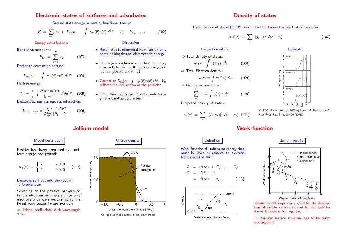
Example

-8 -6 -4 -2 00

1

2

3

4

E-EF @eVD

Layer 30

1

2

3

4

LD

OS@s

tate

s�eVD

Layer 20

1

2

3

4 Layer 1

d-LDOS of the three top Pd(210) layers (M. Lischka and A.

Groß, Phys. Rev. B 65, 075420 (2002))

Jellium model

Model description

Positive ion charges replaced by a uni-form charge background:

n+(~r) =

{

n, z ≤ 0

0, z > 0. (112)

Electrons spill out into the vacuum⇒ Dipole layer

Screening of the positive backgroundby the electrons incomplete since onlyelectrons with wave vectors up to theFermi wave vector kF are available

⇒ Friedel oscillations with wavelengthπ/kF

Charge density

1.0

0.5

0−1.0 −0.5 0.5 1.00

r = 5

Positive

background

r = 2

s

sEle

ctro

n d

ensi

ty (

1/n

)

Distance from the surface (1/k )F

−

Charge density at a surface in the jellium model

Work function

Definition

Work function Φ: minimum energy thatmust be done to remove an electronfrom a solid at 0K.

Φ = φ(∞) + EN−1 − EN

Φ = ∆φ − µ

= φ(∞) − εF , (113)

Φ

µ

∆φ

φ( )φ

εEnerg

y

Distance from the surface z

φ( )8

8−(z)

F−

Jellium results

Work

funct

ion (

eV

)

2 3 4 5 6

Wigner−Seitz radius r (a.u.)

2

3

5

4

Experiment

Ion lattice model

Jellium model

Pb

Al

Li

NaK

Rb Cs

Mg

Ag

AuZn Cu

s

Jellium model surprisingly good for the descrip-tion of simple sp-bonded metals, but fails ford-metals such as Au, Ag, Cu, . . .

⇒ Realistic surface structure has to be takeninto account

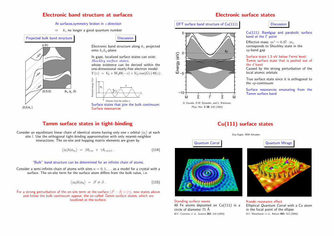
Electronic band structure at surfaces

At surfaces,symmetry broken in z-direction

⇒ kz no longer a good quantum number

Projected bulk band structure

(k ,k ,0)x y

ε

(0,0,0)

(k)

(0,0,k )z

Discussion

Electronic band structure along kz projectedonto kxky-plane

In gaps, localized surface states can exist:Shockley surface states,whose existence can be derived within theone-dimensional nearly-free electron model:V (z) = V0 +W0Θ(−z) + VG cos(Gz) Θ(z) .

0 Distance from the surface z

Pot

enti

al e

nerg

y V

(z)

W0

V0

|VG|

a

Surface states that join the bulk continuum:Surface resonances

Electronic surface states

DFT surface band structure of Cu(111)

MΣ ΣΓ

εF

M

0

5

−10

−5Energ

y (e

V)

A. Euceda, D.M. Bylander, and L. Kleinman,

Phys. Rev. B 28, 528 (1983)

Discussion

Cu(111): Bandgap and parabolic surfaceband at the Γ point

Effective mass: m∗ = 0.37 ·me

corresponds to Shockley state in thesp-band gap

Surface state 1.5 eV below Fermi level:Tamm surface state that is pushed out ofthe d bandCaused by the strong perturbation of thelocal atomic orbitals

True surface state since it is orthogonal tothe sp-continuum

Surface resonances emanating from theTamm surface band

Tamm surface states in tight-binding

Consider an equidistant linear chain of identical atoms having only one s orbital |φl⟩

at eachsite l. Use the orthogonal tight-binding approximation with only nearest-neighbor

interactions. The on-site and hopping matrix elements are given by

⟨

φl|h|φm⟩

= βδl,m + γδl,m±1 . (114)

“Bulk” band structure can be determined for an infinite chain of atoms.

Consider a semi-infinite chain of atoms with sites n = 0, 1, . . . as a model for a crystal with asurface. The on-site term for the surface atom differs from the bulk value, i.e.

⟨

φ0|h|φ0

⟩

= β′ 6= β . (115)

For a strong perturbation of the on-site term at the surface |β′ − β| > |γ|, new states aboveand below the bulk continuum appear, the so-called Tamm surface states, which are

localized at the surface.

Cu(111) surface states

Don Eigler, IBM Almaden

Quantum Corral

Standing surface waves48 Fe atoms deposited on Cu(111) in acircle of diameter 71 AM.F. Crommie et al., Science 262, 218 (1993).

Quantum Mirage

Kondo resonance effectElliptical Quantum Corral with a Co atomin the focal point of the ellipseH.C. Manoharan et al., Nature 403, 512 (2000).

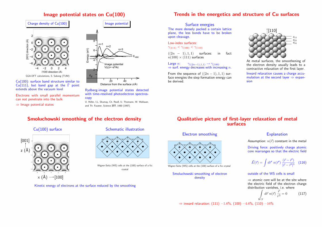
Image potential states on Cu(100)

Charge density of Cu(100)[0

01]

direct

ion (

Å)

[100] direction (Å)

2

0

−2

−4

−6

0 2 4−4 −2

GGA-DFT calculations, S. Sakong (TUM)

Cu(100): surface band structure similar toCu(111), but band gap at the Γ pointextends above the vacuum level

Electrons with small parallel momentumcan not penetrate into the bulk

⇒ Image potential states

Image potential

εF

20 40

2

Distance from the surface z(Å)

εvac

Image potentialV(z)=−e /4z

n=1n=2

n=3

Energ

y (e

V)

6

8

4

2

Rydberg-image potential states detectedwith time-resolved photoelectron spectros-copyU. Hofer, I.L. Shumay, Ch. Reuß, U. Thomann, W. Wallauer,

and Th. Fauster, Science 277, 1480 (1997)

Trends in the energetics and structure of Cu surfaces

Surface energiesThe more densely packed a certain latticeplane, the less bonds have to be brokenupon cleavage.

Low-index surfaces:γ(111) < γ(100) < γ(110)

((2n − 1), 1, 1) surfaces: in factn(100)× (111) surfaces

Large n: γ((2n−1),1,1) → γ(100)

⇒ surf. energy decreases with increasing n.

From the sequence of ((2n − 1), 1, 1) sur-face energies the step formation energy canbe derived.

Relaxations6[110]

d12d23d34

At metal surfaces, the smoothening ofthe electron density usually leads to acontractive relaxation of the first layer.

Inward relaxation causes a charge accu-mulation at the second layer ⇒ expan-sion

Smoluchowski smoothing of the electron density

Cu(100) surface

-4 -2 0 2 4

-6

-4

-2

0

2

x (A) - [100]

z (A)

[001]6

Schematic illustration

+ + + +− − − − −

Wigner-Seitz (WS) cells at the (100) surface of a fcc

crystal

Kinetic energy of electrons at the surface reduced by the smoothing

Qualitative picture of first-layer relaxation of metalsurfaces

Electron smoothing

+ + + +− − − − −

Wigner-Seitz (WS) cells at the (100) surface of a fcc crystal

Smoluchowski smoothing of electrondensity

Explanation

Assumption: n(~r) constant in the metal

Driving force: positively charge atomiccore rearranges so that the electric field

~E(~r) =

∫

d~r′ n(~r′)(~r − ~r′)|~r − ~r′|3 (116)

outside of the WS cells is small

⇒ atomic core will be at the site wherethe electric field of the electron chargedistribution vanishes, i.e. where

∫

WS

d~r n(~r)~r

r3= 0 (117)

⇒ inward relaxation: (111) −1.6%, (100) −4.6%, (110) −16%

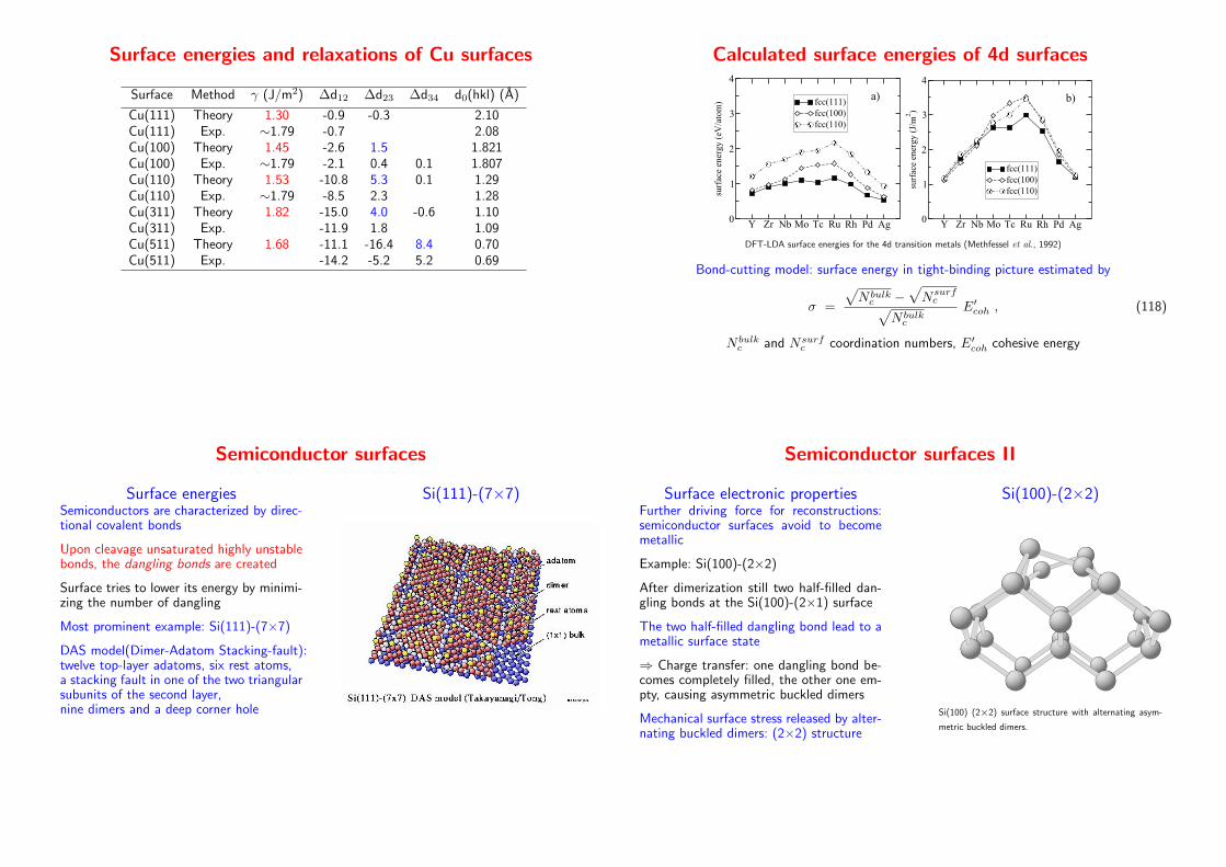
Surface energies and relaxations of Cu surfaces

Surface Method γ (J/m2) ∆d12 ∆d23 ∆d34 d0(hkl) (A)

Cu(111) Theory 1.30 -0.9 -0.3 2.10Cu(111) Exp. ∼1.79 -0.7 2.08Cu(100) Theory 1.45 -2.6 1.5 1.821Cu(100) Exp. ∼1.79 -2.1 0.4 0.1 1.807Cu(110) Theory 1.53 -10.8 5.3 0.1 1.29Cu(110) Exp. ∼1.79 -8.5 2.3 1.28Cu(311) Theory 1.82 -15.0 4.0 -0.6 1.10Cu(311) Exp. -11.9 1.8 1.09Cu(511) Theory 1.68 -11.1 -16.4 8.4 0.70Cu(511) Exp. -14.2 -5.2 5.2 0.69

Calculated surface energies of 4d surfaces

Y Zr Nb Mo Tc Ru Rh Pd Ag0

1

2

3

4

surf

ace

ener

gy (

eV/a

tom

) fcc(111)fcc(100)fcc(110)

a)

Y Zr Nb Mo Tc Ru Rh Pd Ag0

1

2

3

4

surf

ace

ener

gy (

J/m

2 )

fcc(111)fcc(100)fcc(110)

b)

DFT-LDA surface energies for the 4d transition metals (Methfessel et al., 1992)

Bond-cutting model: surface energy in tight-binding picture estimated by

σ =

√

N bulkc −

√

Nsurfc

√

N bulkc

E′coh , (118)

N bulkc and Nsurf

c coordination numbers, E′coh cohesive energy

Semiconductor surfaces

Surface energiesSemiconductors are characterized by direc-tional covalent bonds

Upon cleavage unsaturated highly unstablebonds, the dangling bonds are created

Surface tries to lower its energy by minimi-zing the number of dangling

Most prominent example: Si(111)-(7×7)

DAS model(Dimer-Adatom Stacking-fault):twelve top-layer adatoms, six rest atoms,a stacking fault in one of the two triangularsubunits of the second layer,nine dimers and a deep corner hole

Si(111)-(7×7)

Semiconductor surfaces II

Surface electronic propertiesFurther driving force for reconstructions:semiconductor surfaces avoid to becomemetallic

Example: Si(100)-(2×2)

After dimerization still two half-filled dan-gling bonds at the Si(100)-(2×1) surface

The two half-filled dangling bond lead to ametallic surface state

⇒ Charge transfer: one dangling bond be-comes completely filled, the other one em-pty, causing asymmetric buckled dimers

Mechanical surface stress released by alter-nating buckled dimers: (2×2) structure

Si(100)-(2×2)

Si(100) (2×2) surface structure with alternating asym-

metric buckled dimers.

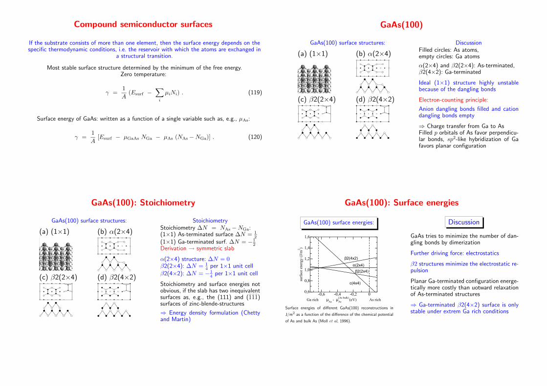
Compound semiconductor surfaces

If the substrate consists of more than one element, then the surface energy depends on thespecific thermodynamic conditions, i.e. the reservoir with which the atoms are exchanged in

a structural transition.

Most stable surface structure determined by the minimum of the free energy.Zero temperature:

γ =1

A(Esurf −

∑

i

µiNi) . (119)

Surface energy of GaAs: written as a function of a single variable such as, e.g., µAs:

γ =1

A[Esurf − µGaAs NGa − µAs (NAs −NGa)] . (120)

GaAs(100)

GaAs(100) surface structures:

(a) (1×1) (b) α(2×4)

(c) β2(2×4) (d) β2(4×2)

DiscussionFilled circles: As atoms,empty circles: Ga atoms

α(2×4) and β2(2×4): As-terminated,β2(4×2): Ga-terminated

Ideal (1×1) structure highly unstablebecause of the dangling bonds

Electron-counting principle:

Anion dangling bonds filled and cationdangling bonds empty

⇒ Charge transfer from Ga to AsFilled p orbitals of As favor perpendicu-lar bonds, sp2-like hybridization of Gafavors planar configuration

GaAs(100): Stoichiometry

GaAs(100) surface structures:

(a) (1×1) (b) α(2×4)

(c) β2(2×4) (d) β2(4×2)

StoichiometryStoichiometry ∆N = NAs −NGa:(1×1) As-terminated surface ∆N = 1

2

(1×1) Ga-terminated surf. ∆N = −12

Derivation → symmetric slab

α(2×4) structure: ∆N = 0β2(2×4): ∆N = 1

4 per 1×1 unit cellβ2(4×2): ∆N = −1

4 per 1×1 unit cell

Stoichiometry and surface energies notobvious, if the slab has two inequivalentsurfaces as, e.g., the (111) and (111)surfaces of zinc-blende-structures

⇒ Energy density formulation (Chettyand Martin)

GaAs(100): Surface energies

GaAs(100) surface energies:

-0,6 -0,4 -0,2 0Ga rich µ

As - µ(As bulk)

As (eV) As rich

0,6

0,8

1,0

1,2

1,4

1,6

surf

ace

ener

gy (

J/m

2 )

β2(4x2)

α(2x4)

β2(2x4)

c(4x4)

Surface energies of different GaAs(100) reconstructions in

J/m2 as a function of the difference of the chemical potential

of As and bulk As (Moll et al, 1996).

Discussion

GaAs tries to minimize the number of dan-gling bonds by dimerization

Further driving force: electrostatics

β2 structures minimize the electrostatic re-pulsion

Planar Ga-terminated configuration energe-tically more costly than uotward relaxationof As-terminated structures

⇒ Ga-terminated β2(4×2) surface is onlystable under extrem Ga rich conditions

Insulator surfaces

NaCl structure

Sodium chloride structure

Ionic surfaces

NaCl structure: Two fcc sublattices trans-lated by a/2(~ex + ~ey + ~ez)

Electrostatic potential outside of a slabstructure:

φ(z →∞) = φG e−2πz a + 2πσ⊥ (121)

σ⊥: dipole moment perpendicular to theplane per unit areaPolar surface highly unstable

Nonpolar surface: electrostatic potentialfalls off very rapidly, surface terminationalmost ideal

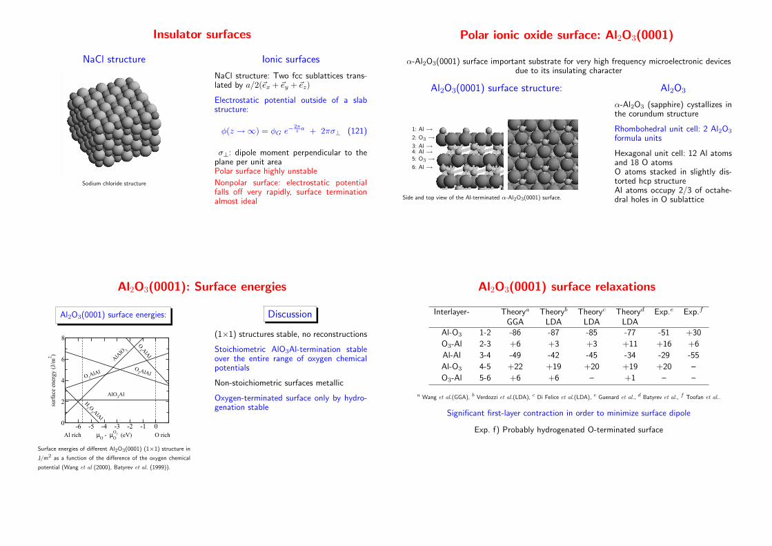
Polar ionic oxide surface: Al2O3(0001)

α-Al2O3(0001) surface important substrate for very high frequency microelectronic devicesdue to its insulating character

Al2O3(0001) surface structure:

1: Al →2: O3 →3: Al →4: Al →5: O3 →6: Al →

Side and top view of the Al-terminated α-Al2O3(0001) surface.

Al2O3

α-Al2O3 (sapphire) cystallizes inthe corundum structure

Rhombohedral unit cell: 2 Al2O3

formula units

Hexagonal unit cell: 12 Al atomsand 18 O atomsO atoms stacked in slightly dis-torted hcp structureAl atoms occupy 2/3 of octahe-dral holes in O sublattice

Al2O3(0001): Surface energies

Al2O3(0001) surface energies:

-6 -5 -4 -3 -2 -1 0Al rich µ

O - µO

2

O (eV) O rich

0

2

4

6

8

surf

ace

ener

gy (

J/m

2 )

AlO3Al

AlAlO 3

O 1AlAl

O2 AlAl

O3 A

lAl

H3 O

3 AlAl

Surface energies of different Al2O3(0001) (1×1) structure in

J/m2 as a function of the difference of the oxygen chemical

potential (Wang et al (2000), Batyrev et al. (1999)).

Discussion

(1×1) structures stable, no reconstructions

Stoichiometric AlO3Al-termination stableover the entire range of oxygen chemicalpotentials

Non-stoichiometric surfaces metallic

Oxygen-terminated surface only by hydro-genation stable

Al2O3(0001) surface relaxations

Interlayer- Theorya Theoryb Theoryc Theoryd Exp.e Exp.f

GGA LDA LDA LDAAl-O3 1-2 -86 -87 -85 -77 -51 +30

O3-Al 2-3 +6 +3 +3 +11 +16 +6

Al-Al 3-4 -49 -42 -45 -34 -29 -55

Al-O3 4-5 +22 +19 +20 +19 +20 –

O3-Al 5-6 +6 +6 – +1 – –

a Wang et al.(GGA), b Verdozzi et al.(LDA), c Di Felice et al.(LDA), e Guenard et al., d Batyrev et al., f Toofan et al..

Significant first-layer contraction in order to minimize surface dipole

Exp. f) Probably hydrogenated O-terminated surface

Al2O3(0001) surface reconstructions at highertemperatures

Above T = 1350 K, oxygen evaporates from the top layers

⇒ Complex Al-rich structures addressed with empirical potentialshexagonal and square arrangement of Al atoms in top layer

(100)−like

(111)−like

(111)−like

(3√

3× 3√

3)r30◦ reconstructed α-Al2O3(0001) surface obtained by simulations using empirical potentials

I. Vilfan et al., Surf. Sci. 505, L215 (2002)

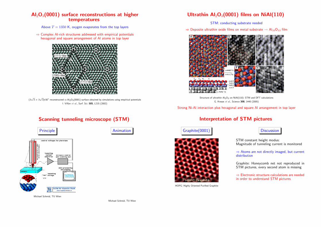
Ultrathin Al2O3(0001) films on NiAl(110)

STM: conducting substrate needed

⇒ Deposite ultrathin oxide films on metal substrate → Al10O13 film

Structure of ultrathin Al2O3 on NiAl(110): STM and DFT calculations

G. Kresse et al., Science 308, 1440 (2005)

Strong Ni-Al interaction plus hexagonal and square Al arrangement in top layer

Scanning tunneling microscope (STM)

Principle

Michael Schmid, TU Wien

Animation

Michael Schmid, TU Wien

Interpretation of STM pictures

Graphite(0001)

HOPG: Highly Oriented Purified Graphite

Discussion

STM constant height modus:Magnitude of tunneling current is monitored

⇒ Atoms are not directly imaged, but currentdistribution

Graphite: Honeycomb net not reproduced inSTM pictures, every second atom is missing

⇒ Electronic structure calculations are neededin order to understand STM pictures

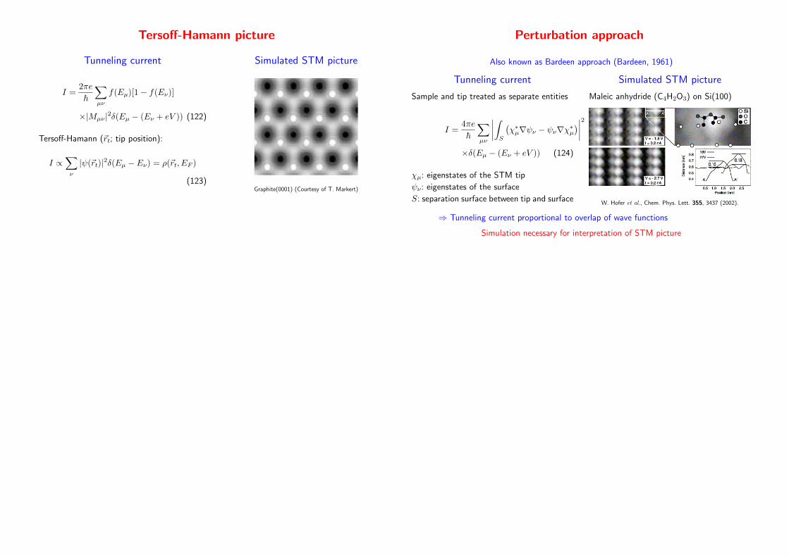
Tersoff-Hamann picture

Tunneling current

I =2πe

~

∑

µν

f(Eµ)[1− f(Eν)]

×|Mµν|2δ(Eµ − (Eν + eV )) (122)

Tersoff-Hamann (~rt; tip position):

I ∝∑

ν

|ψ(~rt)|2δ(Eµ − Eν) = ρ(~rt, EF )

(123)

Simulated STM picture

Graphite(0001) (Courtesy of T. Markert)

Perturbation approach

Also known as Bardeen approach (Bardeen, 1961)

Tunneling current

Sample and tip treated as separate entities

I =4πe

~

∑

µν

∣

∣

∣

∣

∫

S

(

χ∗µ∇ψν − ψν∇χ∗µ)

∣

∣

∣

∣

2

×δ(Eµ − (Eν + eV )) (124)

χµ: eigenstates of the STM tip

ψν: eigenstates of the surface

S: separation surface between tip and surface

Simulated STM picture

Maleic anhydride (C4H2O3) on Si(100)

W. Hofer et al., Chem. Phys. Lett. 355, 3437 (2002).

⇒ Tunneling current proportional to overlap of wave functions

Simulation necessary for interpretation of STM picture