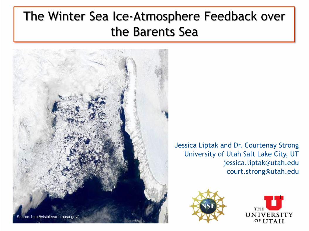
The Winter Sea Ice-Atmosphere Feedback over

the Barents Sea

Jessica Liptak and Dr. Courtenay Strong

University of Utah Salt Lake City, UT

jessica.liptak@utah.edu

court.strong@utah.edu

Source: http://visibleearth.nasa.gov/

1

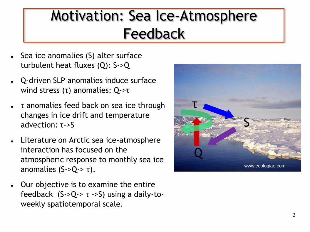
Sea ice anomalies (S) alter surface

turbulent heat fluxes (Q): S->Q

Q-driven SLP anomalies induce surface

wind stress (τ) anomalies: Q->τ

τ anomalies feed back on sea ice through

changes in ice drift and temperature

advection: τ->S

Literature on Arctic sea ice-atmosphere

interaction has focused on the

atmospheric response to monthly sea ice

anomalies (S->Q-> τ).

Our objective is to examine the entire

feedback (S->Q-> τ ->S) using a daily-to-

weekly spatiotemporal scale.

Motivation: Sea Ice-Atmosphere

Feedback

2

www.ecologiae.com

Q

S

τ

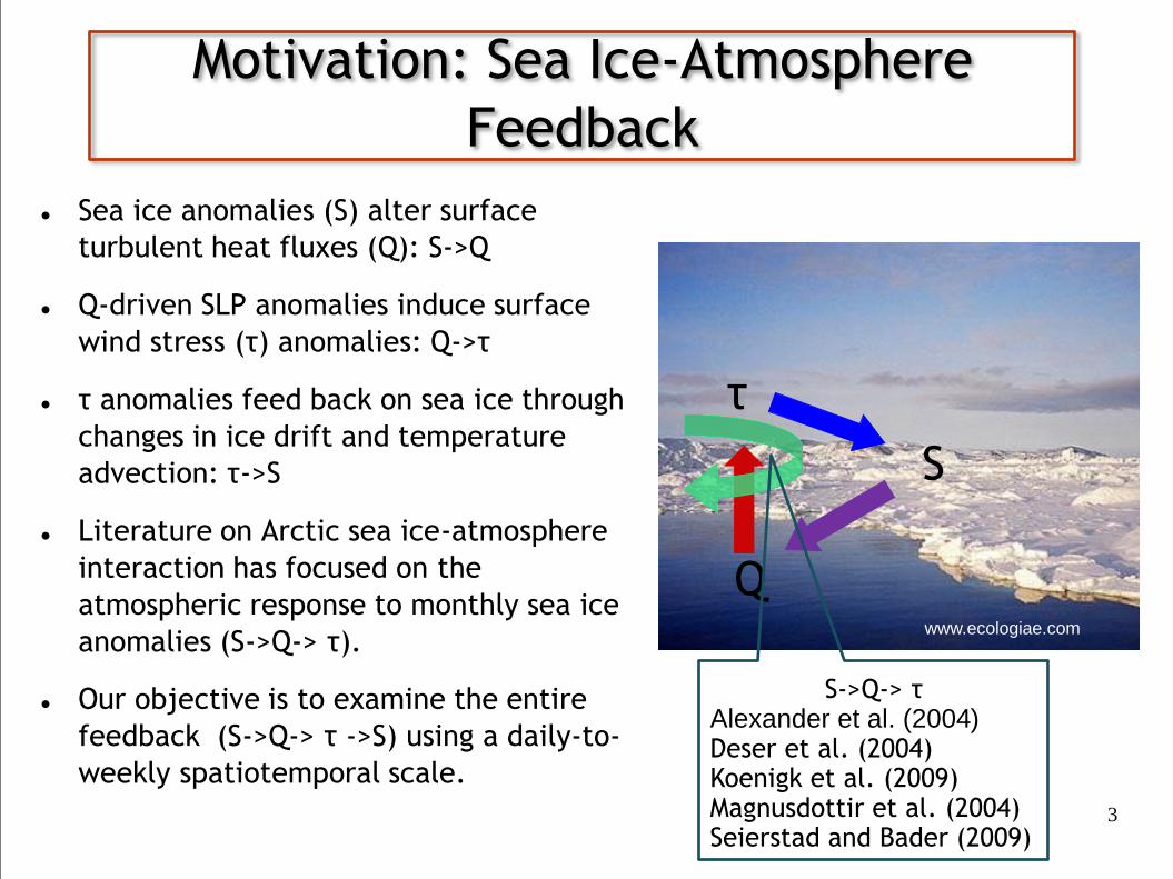
Sea ice anomalies (S) alter surface

turbulent heat fluxes (Q): S->Q

Q-driven SLP anomalies induce surface

wind stress (τ) anomalies: Q->τ

τ anomalies feed back on sea ice through

changes in ice drift and temperature

advection: τ->S

Literature on Arctic sea ice-atmosphere

interaction has focused on the

atmospheric response to monthly sea ice

anomalies (S->Q-> τ).

Our objective is to examine the entire

feedback (S->Q-> τ ->S) using a daily-to-

weekly spatiotemporal scale.

Motivation: Sea Ice-Atmosphere

Feedback

3

www.ecologiae.com www.ecologiae.com

Q

S

τ

S->Q-> τ Alexander et al. (2004) Deser et al. (2004) Koenigk et al. (2009) Magnusdottir et al. (2004) Seierstad and Bader (2009)

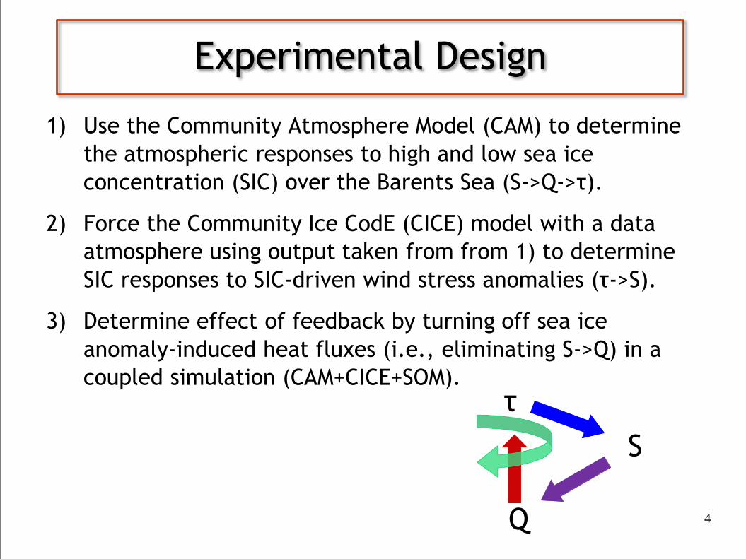
1) Use the Community Atmosphere Model (CAM) to determine

the atmospheric responses to high and low sea ice

concentration (SIC) over the Barents Sea (S->Q->τ).

2) Force the Community Ice CodE (CICE) model with a data

atmosphere using output taken from from 1) to determine

SIC responses to SIC-driven wind stress anomalies (τ->S).

3) Determine effect of feedback by turning off sea ice

anomaly-induced heat fluxes (i.e., eliminating S->Q) in a

coupled simulation (CAM+CICE+SOM).

Experimental Design

4 Q

S

τ

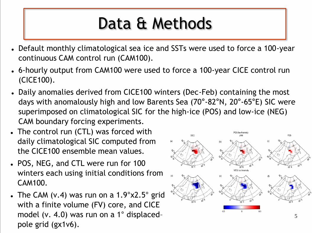
Data & Methods

The control run (CTL) was forced with

daily climatological SIC computed from

the CICE100 ensemble mean values.

POS, NEG, and CTL were run for 100

winters each using initial conditions from

CAM100.

The CAM (v.4) was run on a 1.9°x2.5° grid

with a finite volume (FV) core, and CICE

model (v. 4.0) was run on a 1° displaced–

pole grid (gx1v6).

5

Default monthly climatological sea ice and SSTs were used to force a 100-year

continuous CAM control run (CAM100).

6-hourly output from CAM100 were used to force a 100-year CICE control run

(CICE100).

Daily anomalies derived from CICE100 winters (Dec-Feb) containing the most

days with anomalously high and low Barents Sea (70°-82°N, 20°-65°E) SIC were

superimposed on climatological SIC for the high-ice (POS) and low-ice (NEG)

CAM boundary forcing experiments.

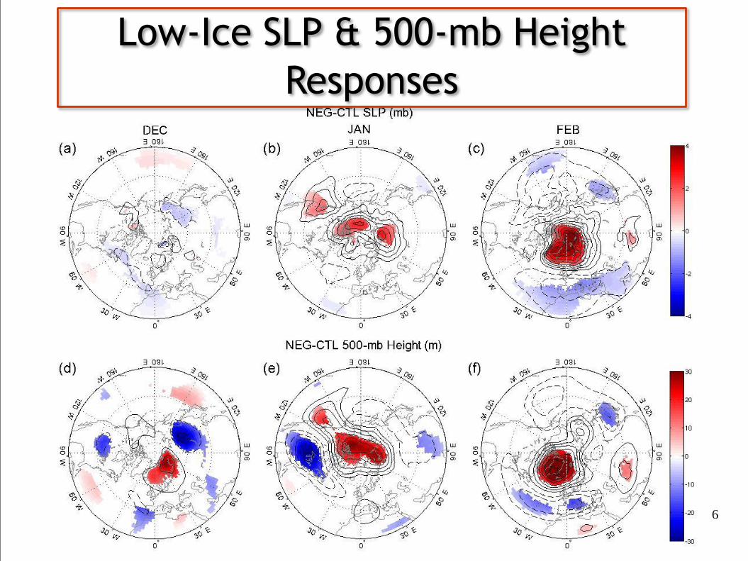
Low-Ice SLP & 500-mb Height

Responses

6

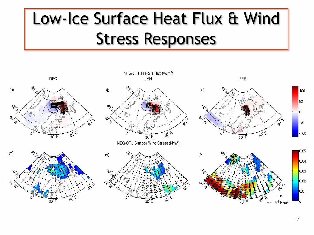
Low-Ice Surface Heat Flux & Wind

Stress Responses

7

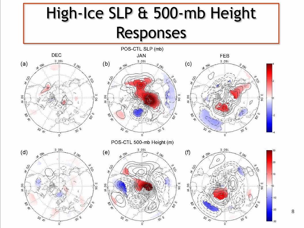
High-Ice SLP & 500-mb Height

Responses

8

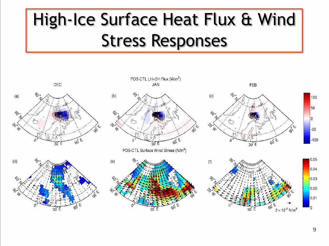
High-Ice Surface Heat Flux & Wind

Stress Responses

9

10

Summary

Monthly mean responses to the high- and low-ice forcing showed

opposite-signed surface wind stress and turbulent heat flux anomalies.

The large-scale high- and low-ice SLP and 500-mb responses were

remarkably similar.

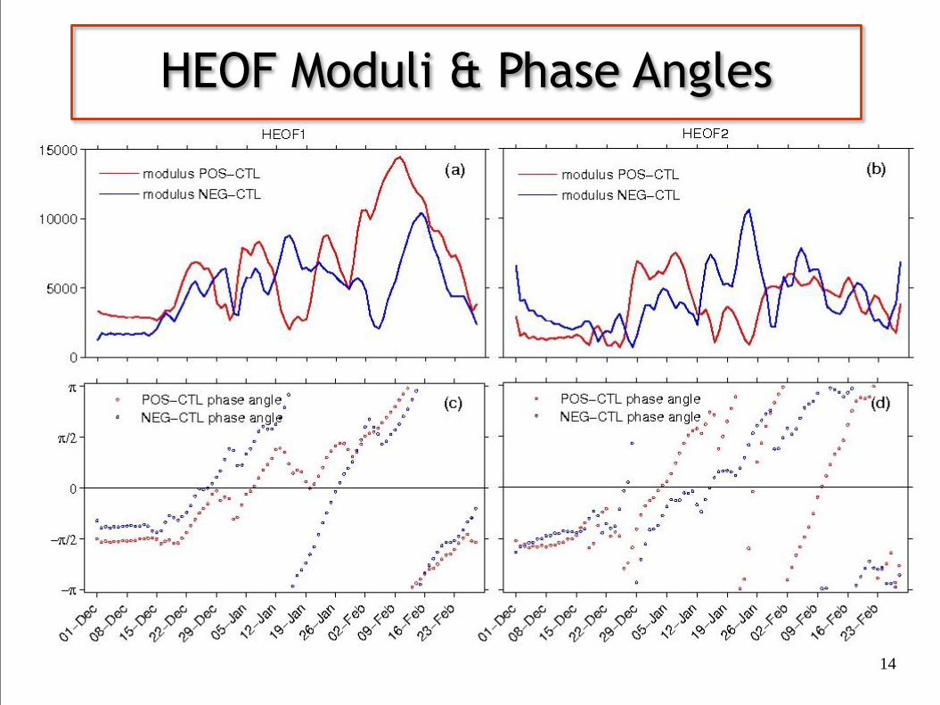
Hilbert Empirical Orthogonal Functions (HEOFs) of the SLP responses

show propagating features resembling the AO/NAO and wave 2

patterns.

The feedback of the atmosphere onto the ice is currently being

analyzed from CICE runs forced with output from the CAM control and

experiments.

Preliminary results suggest the sign of the ice-atmosphere

feedback depends on the sign of the ice anomaly over the

Barents Sea.

Acknowledgments

This research was supported by the National Science Foundation

Arctic Sciences Division grant 1022485.

Provision of computer infrastructure by the Center for High

Performance Computing at the University of Utah is gratefully

acknowledged.

11

Alexander, M. A., U.S. Bhatt, J. E. Walsh, M. S. Timlin, J. S. Miller, and J. D. Scott,

2004: The atmospheric response to realistic Arctic sea ice anomalies in an AGCM

during winter J.Clim, 17, 890-905.

Deser, C., G. Magnusdottir, R. Saravanan, and A. S., Phillips, 2004: The effects of

North Atlantic SST and sea-ice anomalies on the winter circulation in CCM3 Part II:

Direct and indirect components of the Hurrell, J. W., J. H. Hack, D. Shea, J. M.

Caron, and J. Rosinski (2008): A new sea surface temperature and sea ice boundary

dataset for the Community Atmosphere Model, J. Clim., 21, 5145-5153, doi:

10.1175/2008JCLI2292.1.

Koenigk, T., U. Mikolajewicz, J. H. Jungclaus, andbA. Kroll, A, 2009: Sea ice in the

Barents Sea: Seasonal to interannual variability and climate feedbacks in a global

coupled model, Clim. Dyn., 32, 1119-1138

Magnusdottir, G., C. Deser, and R. Saravanan, 2004: The effects of North Atlantic

SST and sea ice anomalies on the winter circulation in CCM3. Part I: main features

and storm track characteristics of the response, J.Clim., 17, 857-876.

Seierstad, I. and J. Bader, 2009: Impact of a projected future Arctic Sea Ice

reduction on extratropical storminess and the NAO, Clim. Dyn., 33, 937-943.

References

12

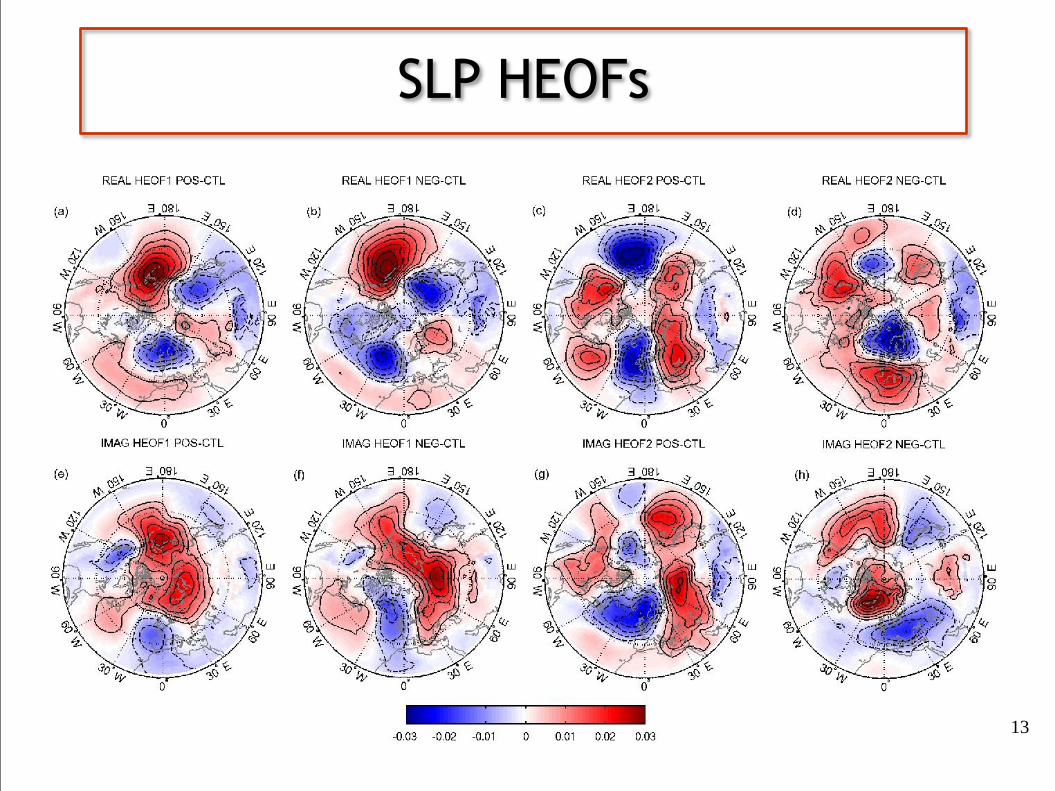
13

SLP HEOFs

14

HEOF Moduli & Phase Angles