THE WEYL ALGEBRAS

David Cock

Supervisor: Dr. Daniel Chan

School of Mathematics,

The University of New South Wales.

November 2004

Submitted in partial fulfillment of the requirements of the degree of

Bachelor of Science with Honours

Contents

Chapter 1 Introduction 1

Chapter 2 Basic Results 3

Chapter 3 Gradings and Filtrations 16

Chapter 4 Gelfand-Kirillov Dimension 21

Chapter 5 Automorphisms of A1 29

References 53

i

Chapter 1

Introduction

An important result in single-variable calculus is the so-called product rule. That

is, for two polynomials (or more generally, functions) f(x), g(x) : R → R:

δ

δx(fg) = (

δ

δxf)g + f(

δ

δxg)

It turns out that this formula, which is firmly rooted in calculus has very inter-

esting algebraic properties. If k[x] denotes the ring of polynomials in one variable

over a characteristic 0 field k, differentiation (in the variable x) can be considered as

a map δ : k[x] → k[x]. It is relatively straighforward to verify that the map δ is in

fact a k-linear vector space endomorphism of k[x]. Similarly, we can define another

k-linear endomorphism X by left multiplication by x ie. X(f) = xf . Consider the

expression (δ ·X)f(x). Expanding this gives:

(δ ·X)f(x) = δ(xf(x))

applying the product rule gives

(δ ·X)f(x) = δ(x)f(x) + xδf(x)

= f(x) + (X · δ)f(x)

1

noting the common factor of f(x) gives us the relation (this time in the ring of

k-linear endomorphisms of k[x]):

δ ·X = X · δ + 1

where 1 is the identity map. This is the defining relation of the first Weyl algebra

which can be viewed as the ring of differential operators on k[x] with polynomial

coefficients. There also exist higher order Weyl algebras related to the polynomial

ring in n variables.

The Weyl algebras arise in a number of contexts, notably as a quotient of the

universal enveloping algebra of certain finite-dimensional Lie algebras (arising from

the Heisenberg group) which have links to quantum mechanics.

The second chapter of this paper covers some basic results on the Weyl alge-

bras, culminating in the proof that they are simple domains. The third chapter

covers gradings, filtrations and the concept of an associated graded algebra. The

fourth chapter introduces the concept of the Gelfand-Kirillov dimension which is a

useful invariant of finitely-generated associative algebras. The final chapter is an

exposition of a proof published in [1] that characterises the automorphisms of the

first Weyl algebra.

2

Chapter 2

Basic Results

In the following, k will always be a field of characteristic 0 and all ideals are two-

sided unless specifically stated otherwise.

Definition 2.1. Let D be a (not neccessarily commutative) domain. Define A(D)

as the non-commutative algebra over D on the two generators p, q with defining

relation

qp− pq = 1 (2.1)

ie.

A(D) =D < p, q >

(qp− pq − 1)

For a field k of characteristic 0, define the first Weyl algebra over k, denoted

by A1 to be A(k). Define the nth Weyl algebra for n > 1 by An = A(An−1)

(note that this definition assumes that An−1 is a domain, this is proved later). For

convenience assume A0 = k. Note that for n > 1 there are extra (implicit) relations:

qipj − pjqi = 0 for i 6= j ie. the generators of different index commute.

Definition 2.2. Define linear maps X, δ : k[x] → k[x] by X(f) = xf and δ(f) = δfδx

ie. formal differentiation. X and δ generate a sub-algebra of the ring of k-linear

endomorphisms of k[x]. Applying Leibniz’ rule for the differentiation of a product

gives δ ·X = X · δ + 1. Call this algebra A′1.

For n > 1 and 1 ≤ i ≤ n define linear maps Xi, δi : k[x1, . . . , xn] → k[x1, . . . , xn]

by Xi(f) = xif and δi(f) = δfδxi

ie. formal partial differentiation with respect to xi.

3

Once again, differenting the product yields the relations δiXj = Xjδi + 1 if i = j or

δiXj = Xjδi if i 6= j. Call this algebra A′n. Expressed as a quotient:

A′n =

k < X1, . . . , Xn, δ1, . . . , δn >

(δiXj −Xiδj −∆ij)

where

∆ij =

1 i = j

0 otherwise

Lemma 2.3. For any domain D, every x ∈ A(D) can be expressed as∑aijp

iqj

for some finite set {(i, j) ∈ N× N} and aij ∈ D.

Proof. Since p, q generate An over D, every x ∈ An can be expressed as some finite

sum ∑i

bipr(i,1)qs(i,1) . . . pr(i,ni)qs(i,ni)

where bi ∈ D,ni ∈ Z+ and the leading or trailing coefficent (r(i,1) and s(i,ni) re-

spectively) may be 0. Note that p and q both commute with elements of the base

domain D.

For a monomial product term M , define #p(M) to be the number of p terms

appearing in M . Define #q(M) similarly. Let I(M) be the number of ‘inversions’

in the term M . That is, the sum over every q term in M of the number of p terms

which occur to the right. For example:

I(pmqn) = I(λ ∈ k) = 0

I(qp) = 1

I(q2p) = I(qp2) = 2

I(q2p2) = I(qp4) = 4

Define I (∑

iMi) to be maxi (I(Mi)).

Let R =∑

iMi be a represention of x in the form described above. If I(R) > 0,

then for at least one monomial term Mi we must have I(Mi) > 0. Thus the

4

monomial Mi must contain at least one factor of the form qp ie. Mi = AqpB

where A may be in k and B may be 1. Pick one such term and apply the identity

qp = pq + 1 to give:

M ′i = biApqB + biAB

calculating gives:

I(M ′i) = max(I(ApqB), I(AB))

= max(I(mi)− 1, I(mi)− (#q(A) + #p(B))− 1)

clearly therefore, I(M ′i) = I(Mi)− 1.

Inductively therefore, the sequence of manipulations Mi → M ′i must terminate

in some M∗i with I(M∗

i ) = 0. Applying this to each term of R gives a representation

in the required form.

Corollary 2.3.1. Any x ∈ An can be expressed as

∑ai1...inj1...jnp

i11 . . . p

inn q

j11 . . . qjn

n

Proof. Since k is a domain, the result is true for n = 1. An is defined recursively as

A(An−1). Assuming that An−1 is a domain (again, this is proved shortly) and that

the result holds for n− 1, the result follows by induction on n since the generators

of different index commute.

Lemma 2.4. Every x ∈ A′n can be expressed as

∑aX i1

1 . . . X inn δ

i11 . . . δ

inn for some

finite set {(i, j) ∈ N× N}.

Proof. By writing A′n recursively as A′

n−1 < Xn, δn > and using the relation δnXn =

Xnδn + 1, the result follows as for (2.3.1).

Lemma 2.5. The k-linear map φ : An → A′n defined by φ(pi) = Xi and φ(qi) = δi

is an algebra homomorphism.

5

Proof. By the universal property, it suffices to check the images of the defining

relations qipi − piqi − 1 and qipj − pjqi for i 6= j:

φ(qipi − piqi − 1) = δiXi −Xiδi − 1 = 0

φ(qipj − pjqi) = δiXj −Xjδi = 0

Lemma 2.6. For any element of A′n, the representation given in lemma 2.4 is

unique.

Proof. Suppose that an element x ∈ A′n has two distinct representations

∑ai1...inj1...jnX

i11 . . . X in

n δj11 . . . δjn

n

=∑

bi1...inj1...jnXi11 . . . X in

n δj11 . . . δjn

n

Cancel all equal terms in the above sums to give two differential operators (A, B)

with coefficients ai1...inj1...jn and bi1...inj1...jn such that ai1...inj1...jn 6= bi1...inj1...jn for all

i1 . . . inj1 . . . jn . For each 1 ≤ k ≤ n, pick j∗k to be minimal with respect to the

property that ai1...inj1∗...jk∗jk+1...jn and bi1...inj1∗...jk

∗jk+1...jn appear as coefficients of A

and B respectively, for some i1 . . . in, jk+1 . . . jn. Let p = xj∗11 . . . x

j∗nn ∈ k[x1, . . . , xn].

Apply the operators A and B to p.

Ap =∑

ai1...inj1...jnXi11 . . . X in

n δj11 . . . δjn

n xj∗11 . . . xj∗n

n

Bp =∑

bi1...inj1...jnXi11 . . . X in

n δj11 . . . δjn

n xj∗11 . . . xj∗n

n

Consider a single term of the above sums:

ta = ai1...inj1...jnXi11 . . . X in

n δj11 . . . δjn

n xj∗11 . . . xj∗n

n

tb = bi1...inj1...jnXi11 . . . X in

n δj11 . . . δjn

n xj∗11 . . . xj∗n

n

6

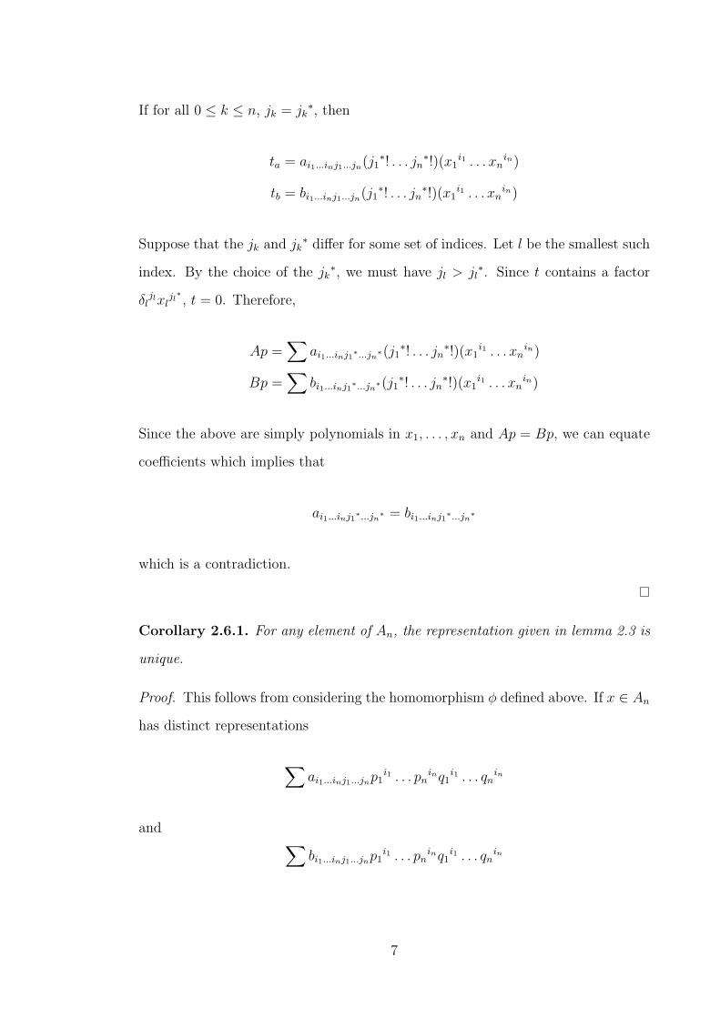
If for all 0 ≤ k ≤ n, jk = jk∗, then

ta = ai1...inj1...jn(j1∗! . . . jn

∗!)(x1i1 . . . xn

in)

tb = bi1...inj1...jn(j1∗! . . . jn

∗!)(x1i1 . . . xn

in)

Suppose that the jk and jk∗ differ for some set of indices. Let l be the smallest such

index. By the choice of the jk∗, we must have jl > jl

∗. Since t contains a factor

δljlxl

jl∗, t = 0. Therefore,

Ap =∑

ai1...inj1∗...jn∗(j1

∗! . . . jn∗!)(x1

i1 . . . xnin)

Bp =∑

bi1...inj1∗...jn∗(j1

∗! . . . jn∗!)(x1

i1 . . . xnin)

Since the above are simply polynomials in x1, . . . , xn and Ap = Bp, we can equate

coefficients which implies that

ai1...inj1∗...jn∗ = bi1...inj1∗...jn

∗

which is a contradiction.

Corollary 2.6.1. For any element of An, the representation given in lemma 2.3 is

unique.

Proof. This follows from considering the homomorphism φ defined above. If x ∈ An

has distinct representations

∑ai1...inj1...jnp1

i1 . . . pninq1

i1 . . . qnin

and ∑bi1...inj1...jnp1

i1 . . . pninq1

i1 . . . qnin

7

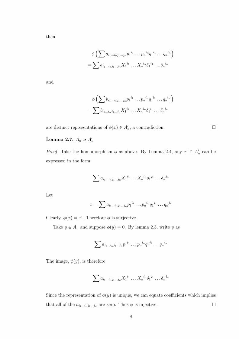
then

φ(∑

ai1...inj1...jnp1i1 . . . pn

inq1i1 . . . qn

in)

=∑

ai1...inj1...jnX1i1 . . . Xn

inδ1i1 . . . δn

in

and

φ(∑

bi1...inj1...jnp1i1 . . . pn

inq1i1 . . . qn

in)

=∑

bi1...inj1...jnX1i1 . . . Xn

inδ1i1 . . . δn

in

are distinct representations of φ(x) ∈ A′n, a contradiction.

Lemma 2.7. An ' A′n

Proof. Take the homomorphism φ as above. By Lemma 2.4, any x′ ∈ A′n can be

expressed in the form

∑ai1...inj1...jnX1

i1 . . . Xninδ1

j1 . . . δnjn

Let

x =∑

ai1...inj1...jnp1i1 . . . pn

inq1j1 . . . qn

jn

Clearly, φ(x) = x′. Therefore φ is surjective.

Take y ∈ An and suppose φ(y) = 0. By lemma 2.3, write y as

∑ai1...inj1...jnp1

i1 . . . pninq1

j1 . . . qnjn

The image, φ(y), is therefore

∑ai1...inj1...jnX1

i1 . . . Xninδ1

j1 . . . δnjn

Since the representation of φ(y) is unique, we can equate coefficients which implies

that all of the ai1...inj1...jn are zero. Thus φ is injective.

8

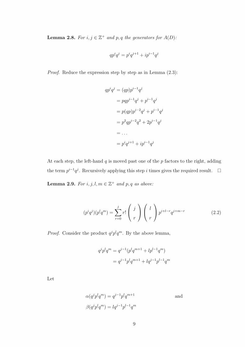
Lemma 2.8. For i, j ∈ Z+ and p, q the generators for A(D):

qpiqj = piqj+1 + ipi−1qj

Proof. Reduce the expression step by step as in Lemma (2.3):

qpiqj = (qp)pi−1qj

= pqpi−1qj + pi−1qj

= p(qp)pi−2qj + pi−1qj

= p2qpi−2q2 + 2pi−1qj

= . . .

= piqj+1 + ipi−1qj

At each step, the left-hand q is moved past one of the p factors to the right, adding

the term pi−1qj. Recursively applying this step i times gives the required result.

Lemma 2.9. For i, j, l,m ∈ Z+ and p, q as above:

(piqj)(plqm) =

j∑r=0

r!

j

r

l

r

pi+l−rqj+m−r (2.2)

Proof. Consider the product qjplqm. By the above lemma,

qjplqm = qj−1(plqm+1 + lpl−1qm)

= qj−1plqm+1 + lqj−1pl−1qm

Let

α(qjplqm) = qj−1plqm+1 and

β(qjplqm) = lqj−1pl−1qm

9

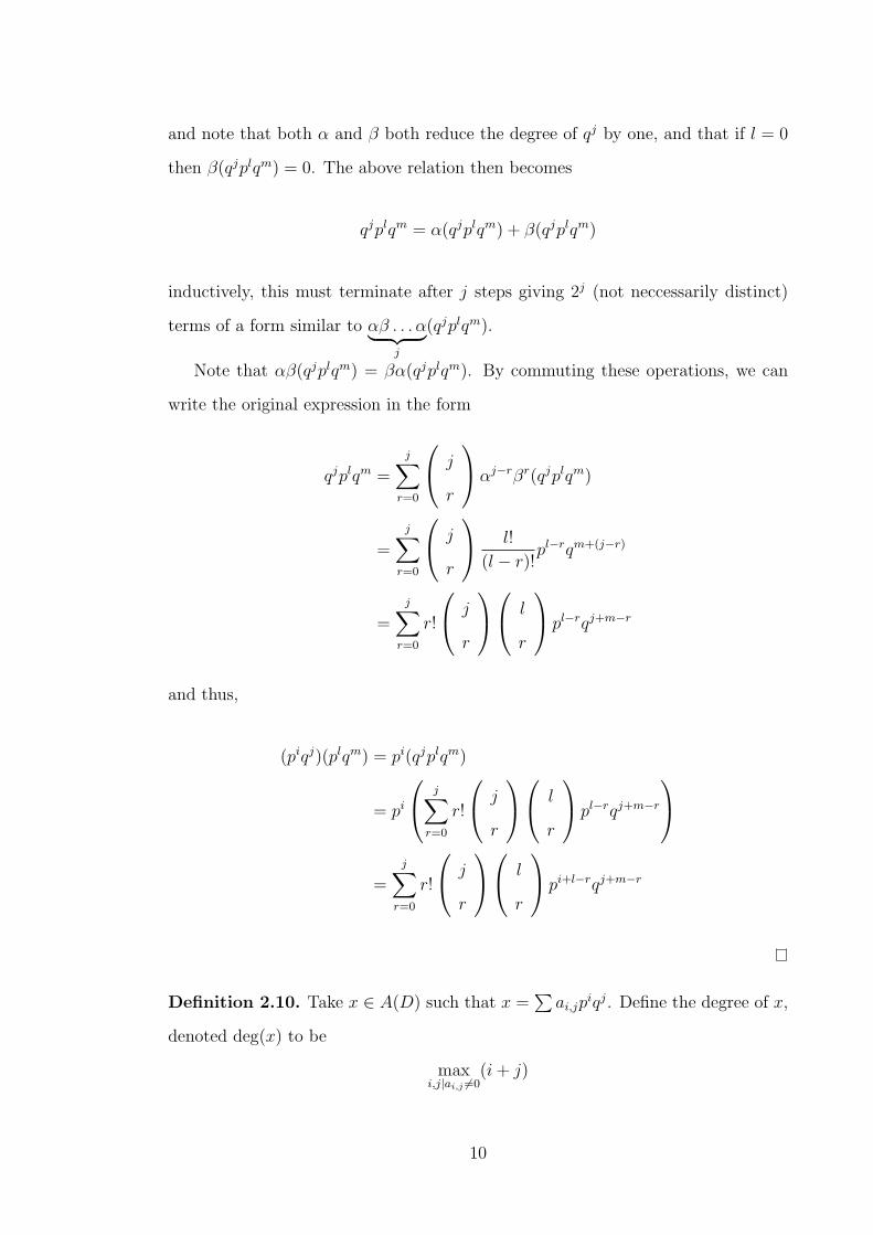
and note that both α and β both reduce the degree of qj by one, and that if l = 0

then β(qjplqm) = 0. The above relation then becomes

qjplqm = α(qjplqm) + β(qjplqm)

inductively, this must terminate after j steps giving 2j (not neccessarily distinct)

terms of a form similar to αβ . . . α︸ ︷︷ ︸j

(qjplqm).

Note that αβ(qjplqm) = βα(qjplqm). By commuting these operations, we can

write the original expression in the form

qjplqm =

j∑r=0

j

r

αj−rβr(qjplqm)

=

j∑r=0

j

r

l!

(l − r)!pl−rqm+(j−r)

=

j∑r=0

r!

j

r

l

r

pl−rqj+m−r

and thus,

(piqj)(plqm) = pi(qjplqm)

= pi

j∑r=0

r!

j

r

l

r

pl−rqj+m−r

=

j∑r=0

r!

j

r

l

r

pi+l−rqj+m−r

Definition 2.10. Take x ∈ A(D) such that x =∑ai,jp

iqj. Define the degree of x,

denoted deg(x) to be

maxi,j|ai,j 6=0

(i+ j)

10

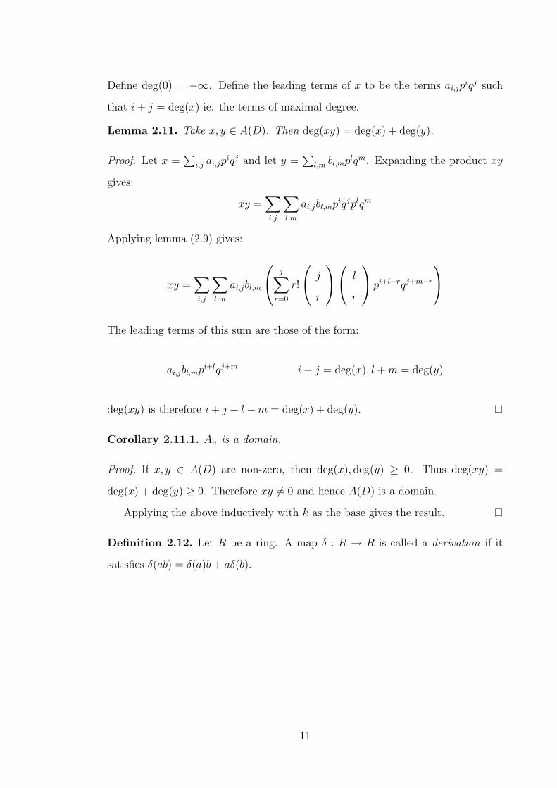
Define deg(0) = −∞. Define the leading terms of x to be the terms ai,jpiqj such

that i+ j = deg(x) ie. the terms of maximal degree.

Lemma 2.11. Take x, y ∈ A(D). Then deg(xy) = deg(x) + deg(y).

Proof. Let x =∑

i,j ai,jpiqj and let y =

∑l,m bl,mp

lqm. Expanding the product xy

gives:

xy =∑i,j

∑l,m

ai,jbl,mpiqjplqm

Applying lemma (2.9) gives:

xy =∑i,j

∑l,m

ai,jbl,m

j∑r=0

r!

j

r

l

r

pi+l−rqj+m−r

The leading terms of this sum are those of the form:

ai,jbl,mpi+lqj+m i+ j = deg(x), l +m = deg(y)

deg(xy) is therefore i+ j + l +m = deg(x) + deg(y).

Corollary 2.11.1. An is a domain.

Proof. If x, y ∈ A(D) are non-zero, then deg(x), deg(y) ≥ 0. Thus deg(xy) =

deg(x) + deg(y) ≥ 0. Therefore xy 6= 0 and hence A(D) is a domain.

Applying the above inductively with k as the base gives the result.

Definition 2.12. Let R be a ring. A map δ : R → R is called a derivation if it

satisfies δ(ab) = δ(a)b+ aδ(b).

11

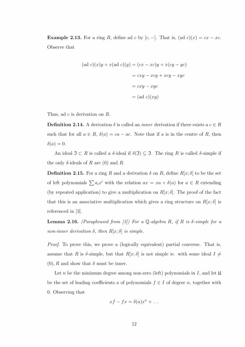
Example 2.13. For a ring R, define ad c by [c,−]. That is, (ad c)(x) = cx − xc.

Observe that

(ad c)(x)y + x(ad c)(y) = (cx− xc)y + x(cy − yc)

= cxy − xcy + xcy − xyc

= cxy − xyc

= (ad c)(xy)

Thus, ad c is derivation on R.

Definition 2.14. A derivation δ is called an inner derivation if there exists a c ∈ R

such that for all a ∈ R, δ(a) = ca − ac. Note that if a is in the centre of R, then

δ(a) = 0.

An ideal I ⊂ R is called a δ-ideal if δ(I) ⊆ I. The ring R is called δ-simple if

the only δ-ideals of R are (0) and R.

Definition 2.15. For a ring R and a derivation δ on R, define R[x; δ] to be the set

of left polynomials∑aix

i with the relation ax = xa + δ(a) for a ∈ R extending

(by repeated application) to give a multiplication on R[x; δ]. The proof of the fact

that this is an associative multiplication which gives a ring structure on R[x; δ] is

referenced in [3].

Lemma 2.16. (Paraphrased from [3]) For a Q-algebra R, if R is δ-simple for a

non-inner derivation δ, then R[x; δ] is simple.

Proof. To prove this, we prove a (logically equivalent) partial converse. That is,

assume that R is δ-simple, but that R[x; δ] is not simple ie. with some ideal I 6=

(0), R and show that δ must be inner.

Let n be the minimum degree among non-zero (left) polynomials in I, and let U

be the set of leading coefficients a of polynomials f ∈ I of degree n, together with

0. Observing that

xf − fx = δ(a)xn + . . .

12

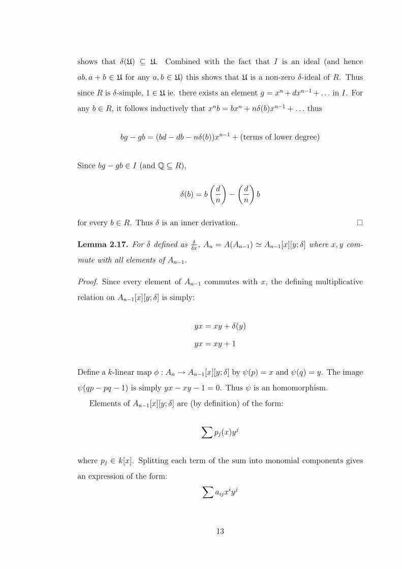
shows that δ(U) ⊆ U. Combined with the fact that I is an ideal (and hence

ab, a + b ∈ U for any a, b ∈ U) this shows that U is a non-zero δ-ideal of R. Thus

since R is δ-simple, 1 ∈ U ie. there exists an element g = xn + dxn−1 + . . . in I. For

any b ∈ R, it follows inductively that xnb = bxn + nδ(b)xn−1 + . . . thus

bg − gb = (bd− db− nδ(b))xn−1 + (terms of lower degree)

Since bg − gb ∈ I (and Q ⊆ R),

δ(b) = b

(d

n

)−(d

n

)b

for every b ∈ R. Thus δ is an inner derivation.

Lemma 2.17. For δ defined as δδx

, An = A(An−1) ' An−1[x][y; δ] where x, y com-

mute with all elements of An−1.

Proof. Since every element of An−1 commutes with x, the defining multiplicative

relation on An−1[x][y; δ] is simply:

yx = xy + δ(y)

yx = xy + 1

Define a k-linear map φ : An → An−1[x][y; δ] by ψ(p) = x and ψ(q) = y. The image

ψ(qp− pq − 1) is simply yx− xy − 1 = 0. Thus ψ is an homomorphism.

Elements of An−1[x][y; δ] are (by definition) of the form:

∑pj(x)y

j

where pj ∈ k[x]. Splitting each term of the sum into monomial components gives

an expression of the form: ∑aijx

iyj

13

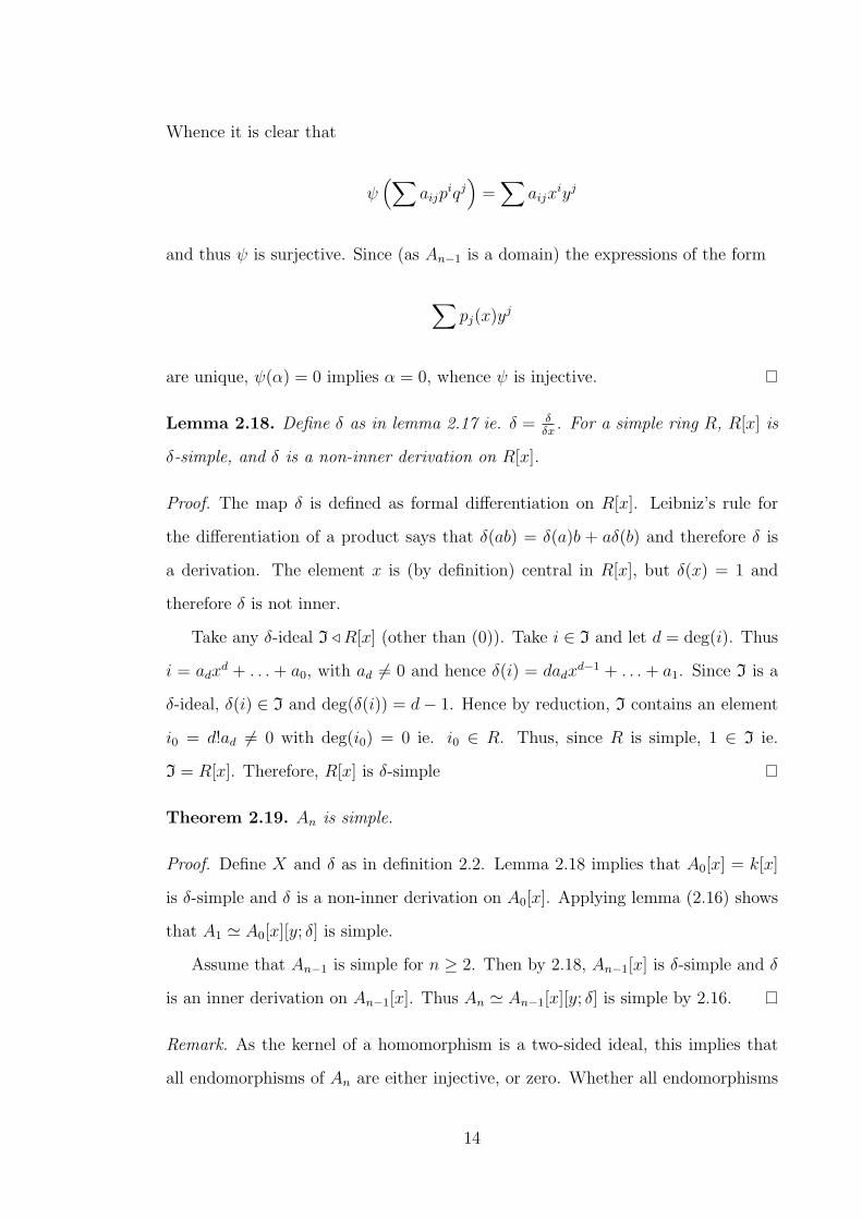
Whence it is clear that

ψ(∑

aijpiqj)

=∑

aijxiyj

and thus ψ is surjective. Since (as An−1 is a domain) the expressions of the form

∑pj(x)y

j

are unique, ψ(α) = 0 implies α = 0, whence ψ is injective.

Lemma 2.18. Define δ as in lemma 2.17 ie. δ = δδx

. For a simple ring R, R[x] is

δ-simple, and δ is a non-inner derivation on R[x].

Proof. The map δ is defined as formal differentiation on R[x]. Leibniz’s rule for

the differentiation of a product says that δ(ab) = δ(a)b + aδ(b) and therefore δ is

a derivation. The element x is (by definition) central in R[x], but δ(x) = 1 and

therefore δ is not inner.

Take any δ-ideal I / R[x] (other than (0)). Take i ∈ I and let d = deg(i). Thus

i = adxd + . . . + a0, with ad 6= 0 and hence δ(i) = dadx

d−1 + . . . + a1. Since I is a

δ-ideal, δ(i) ∈ I and deg(δ(i)) = d− 1. Hence by reduction, I contains an element

i0 = d!ad 6= 0 with deg(i0) = 0 ie. i0 ∈ R. Thus, since R is simple, 1 ∈ I ie.

I = R[x]. Therefore, R[x] is δ-simple

Theorem 2.19. An is simple.

Proof. Define X and δ as in definition 2.2. Lemma 2.18 implies that A0[x] = k[x]

is δ-simple and δ is a non-inner derivation on A0[x]. Applying lemma (2.16) shows

that A1 ' A0[x][y; δ] is simple.

Assume that An−1 is simple for n ≥ 2. Then by 2.18, An−1[x] is δ-simple and δ

is an inner derivation on An−1[x]. Thus An ' An−1[x][y; δ] is simple by 2.16.

Remark. As the kernel of a homomorphism is a two-sided ideal, this implies that

all endomorphisms of An are either injective, or zero. Whether all endomorphisms

14

are also surjective is an important open question, which if proved, would imply an

important result in multi-variable calculus known as the Jacobian conjecture.

15

Chapter 3

Gradings and Filtrations

Definition 3.1. A k-algebra A is N-graded or simply graded, if there exists a set

of subspaces gr(A, i) such that:

gr(A, i).gr(A, j) ⊆ gr(A, i+ j)

and

A =⊕i∈N

gr(A, i)

Elements of the nth graded piece gr(A, n) are called homogeneous of degree n.

Example 3.2. The above statement about homogeneous elements suggests a re-

lation to the idea of an homogeneous polynomial. Take the polynomial algebra

P = k[x1, . . . , xn] and let gr(P, i) be the vector space generated over k by the mono-

mials of degree i in the variables x1, . . . , xn for i ≥ 0 ie. homogeneous polynomials

of degree i. Clearly gr(P, i).gr(P, j) = gr(P, i+ j) for 0 ≤ i, j and P =⊕

i gr(P, i).

This is called the grading by degree and the ith graded component is commonly

denoted k[x1, . . . , xn]i.

Take k[x, y] graded by degree. Take two elements a, b and consider their de-

composition into homogeneous components a =∑

i≥0 ai and b =∑

j≥0 bj with

ai ∈ k[x, y]i and bj ∈ k[x, y]j. The product ab can therefore be decomposed as a

sum of the products of homogeneous terms:

ab =∑i,j≥0

aibj

16

Note that the (i, j)th term of the above sum has degree i + j. This gives a homo-

geneous decomposition of the product:

ab =∑n≥0

∑i+j=n

aibj

Definition 3.3. A k-algebra A is N-filtered or simply filtered, if there exists a set

of subspaces fp(A, i) such that:

fp(A, i) ⊆ fp(A, i+ 1), ∀i ∈ N

1 ∈ fp(A, 0)

fp(A, i).fp(A, j) ⊆ fp(A, i+ j)

A =⋃i∈N

fp(A, i)

Example 3.4. Drawing on Lemma (2.3), any element of the algebra A1 can be

expressed as x =∑

i aipmiqni . Defining deg(x) = maxi{mi+ni} suggests a filtration

of A1 by degree. Define the nth filtered part fp(A1, n) by {x ∈ A1 : deg(x) ≤ n}

ie. not neccessarily homogeneous elements of degree ≤ n. Clearly A1 =⋃

i fp(A1, i)

and 1 ∈ fp(A1, 0). Lemma (2.11) implies that fp(A1, i).fp(A1, j) ⊆ fp(A1, i+ j).

Definition 3.5. Given a filtered algebra A with filtered pieces fp(A, i), define the

associated graded algebra gr(A) corresponding to this filtration to be:

gr(A) =⊕

i

fp(A, i)

fp(A, i− 1)

defining fp(A,−1) = 0 and with multiplication defined on (left)-cosets by:

[x+ fp(A, i− 1)] · [y + fp(A, j − 1)] = [xy + fp(A, i+ j − 1)]

and extended component-wise to multiplication on gr(A).

Lemma 3.6. For a filtered algebra A, gr(A) is an algebra.

17

Proof. • The coset [1+fp(A,−1)] contains only the element 1, which acts as the

multiplicative identity since [x+ fp(A, i− 1)] · [1 + fp(A,−1)] = [x+ fp(A, i+

0− 1)].

• Likewise, the coset [0 + fp(A,−1)] contains only the element 0, which acts as

the additive identity.

• We need to check that the multiplication is well defined. Take the cosets

X = [x+fp(A,m−1)] and Y = [y+fp(A, n−1)] and take the elements a ∈ X

and b ∈ Y . Note that x ∈ fp(A,m) and y ∈ fp(A, n) and write the elements

as:

a = x+ a′ a′ ∈ fp(A,m− 1)

b = y + b′ b′ ∈ fp(A, n− 1)

and form the product:

ab = xy + xb′ + a′y + a′b′

Applying the rule for multiplication of filtered pieces gives:

xy ∈ fp(A,m+ n)

xb′ ∈ fp(A,m+ n− 1)

a′y ∈ fp(A,m+ n− 1)

a′b′ ∈ fp(A,m+ n− 2)

Thus, ab ∈ [xy+fp(A,m+n−1)]. Thus multiplication in gr(A) is well-defined.

• The other ring axioms follow easily from the definition.

18

Lemma 3.7. The associated graded algebra of A1 is k[p, q], the commutative poly-

nomial ring on the variables p and q.

Proof. Take the filtration by degree defined in Example (3.4). Let gr(A) be the

associated graded algebra corresponding to this filtration. Take two homogeneous

elements of gr(A),

x = [a0p0qi + · · ·+ aip

iq0 + fp(A, i− 1)]

and

y = [b0p0qj + · · ·+ bip

jq0 + fp(A, j − 1)]

Where as usual, some of the coefficients a or b may be 0. Take the product xy:

xy = [(a0p0qi + · · ·+ aip

iq0)(b0p0qj + · · ·+ bip

jq0) + fp(A, i+ j − 1)]

Consider a single term of the product:

(ampmqi−m)(bnp

nqj−n) = ambnpmqi−mpnqj−n

Reducing this expression as in 2.3 gives a representation of this term as

ambnpm+nqi+j−m−n + (terms of lower degree)

Thus the product can be expressed as

∑m,n

ambnpm+nqi+j−m−n + (terms of lower degree)

Note that all terms in the left hand sum have degree i+ j. Therefore as a member

of the coset xy + fp(A, i+ j − 1) this is simply

[∑m,n

ambnpm+nqi+j−m−n + fp(A, i+ j − 1)

]

19

Thus multiplication of homogeneous elements behaves exactly as in k[p, q] graded

by degree. Since gr(A) is the direct sum of these homogeneous components, the

multiplication extended to the whole ring is also identical to that in k[p, q].

This allows us to define a homomorphism φ : gr(A) → k[p, q] defined on the

graded components of gr(A) by mapping [x + fp(A, i − 1)] to the leading terms of

the unique representation of x considered as polynomials in k[p, q]i and extended

component-wise to gr(A). This is clearly an homomorphism as shown above. It is

also easy to show that it is bijective.

Definition 3.8. A filtered algebra A for which the associated graded algebra gr(A)

is commutative (eg. An) is called an almost-commutative algebra.

Proposition 3.9. Any finitely-generated almost-commutative algebra A is both left

and right noetherian.

Proof. See [2] proposition 7.1.

Corollary 3.9.1. An is both left and right noetherian.

Remark. It has been proved that an algebra (over k) is almost commutative if and

only if it is a homomorphic image of the universal enveloping algebra of some finite

dimensional Lie algebra over k.

20

Chapter 4

Gelfand-Kirillov Dimension

Let A be a finitely generated k-algebra. Let V be a finite-dimensional generating

subspace for A. That is, if

fp(A, n) = k + V + V 2 + . . .+ Vn

then:

A =⋃n≥0

fp(A, n)

Note that this is a filtration of A with filtered pieces fp(A, n).

Define the function dV (n) : N → R by

dV (n) = dimk(fp(A, n))

Note that if the algebra A is finite dimensional, then there exists some N such that

for all n > N , fp(A, n) = fp(A,N) ie. the function dV (n) becomes stationary.

Note that the function dV (n) depends on A and the choice of generating subspace

V . It would be nice to remove this dependence to get an invariant of the algebra

A. This is done with the following construction.

The idea here is to form an equivalence relation on the functions dV (n) by

comparing their asymptotic growth rate. This turns out to be exactly the right

definition to avoid the dependence on the choice of generating subspace.

21

Definition 4.1. Let Φ denote the set of eventually non-decreasing positive valued

functions f : N → R ie. those for which there exists an n0 ∈ N such that for all n,

f(n) ≥ 0 and for all n ≥ n0

f(n+ 1) ≥ f(n)

Define a relation ≤∗ on Φ by setting f ≤∗ g iff there exist c ∈ R, m ∈ N such

that for all n sufficiently large,

f(n) ≤ cg(mn)

Lemma 4.2. The relation ≤∗ is a preorder relation on the set Φ.

Proof. • (reflexive) Taking c = m = 1 gives f ≤∗ f .

• (transitive) Take f, g, h ∈ Φ and assume that f ≤∗ g and g ≤∗ h ie.

f(n) ≤ c0g(m0n) ∀n > n0

g(n) ≤ c1h(m1n) ∀n > n1

Let n2 = max(n0, n1). Then since f and g are non-decreasing,

f(n) ≤ c0c1h(m0m1n) ∀n > n2

Therefore f ≤∗ h.

Define an equivalence relation on Φ by f ∼ g iff f ≤∗ g and g ≤∗ f . Denote the

partial order induced on the quotient Φ/ ∼ by ≤. For an f ∈ Φ, the equivalence

class G(f) ∈ Φ/ ∼ is called the growth of f .

Lemma 4.3. [2] Let A be a finitely generated k-algebra with finite dimensional

generating subspaces V and W . If dV (n) and dW (n) denote the dimensions of∑ni=0 V

i and∑n

i=0Wi, respectively, then G(dV ) = G(dW ).

22

Proof. Since

A =∞⋃

n=0

(V 0 + . . .+ V n) =∞⋃

n=0

(W 0 + . . .+W n)

there exist positive integers s and t such that

W ⊆s∑

i=0

V i and V ⊆t∑

i=0

W i

Thus dW (n) ≤ dV (sn) and dV (n) ≤ dW (tn), whence dV ∼ dW .

Thus the growth of an algebra A, defined to be G(dV ), is independent of the

choice of generating subspace V .

Example 4.4. Let A = k[p, q], the commutative polynomial ring in two variables.

Take the generating subspace V = kp + kq. Take the basis B1 = {p, q} for V . Let

Bn be the corresponding basis for V n (formed as the product B1 · Bn−1). Assume

that the basis Bn−1 consists of all monomials of degree n− 1 ie.

Bn−1 ={pn−1q0, . . . , p0qn−1

}Then calculating Bn simply gives

Bn ={pnq0, . . . , p1qn−1, pn−1q1, . . . , p0qn

}={pnq0, . . . , p0qn

}Thus, inductively, V n is the space spanned by all (commutative) monomials of

degree n. The set⋃Bn is linearly independent and hence

dV (n) = dimk

n∑i=0

V n

=n∑

i=0

dimk Vn

=1

2(n+ 1)(n+ 2)

23

Thus G(dV ) = G(n2) ie. the polynomial algebra in 2 variables has quadratic growth.

This example extends simply to show that the polynomial algebra in m variables

has degree m polynomial growth.

It will be interesting at this point to try to calculate the growth of the first Weyl

algebra A1. To do so we will need the following lemma:

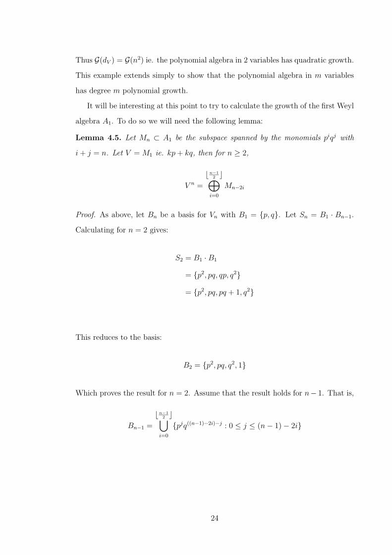
Lemma 4.5. Let Mn ⊂ A1 be the subspace spanned by the monomials piqj with

i+ j = n. Let V = M1 ie. kp+ kq, then for n ≥ 2,

V n =

bn−12 c⊕

i=0

Mn−2i

Proof. As above, let Bn be a basis for Vn with B1 = {p, q}. Let Sn = B1 · Bn−1.

Calculating for n = 2 gives:

S2 = B1 ·B1

= {p2, pq, qp, q2}

= {p2, pq, pq + 1, q2}

This reduces to the basis:

B2 = {p2, pq, q2, 1}

Which proves the result for n = 2. Assume that the result holds for n− 1. That is,

Bn−1 =

bn−12 c⋃

i=0

{pjq((n−1)−2i)−j : 0 ≤ j ≤ (n− 1)− 2i}

24

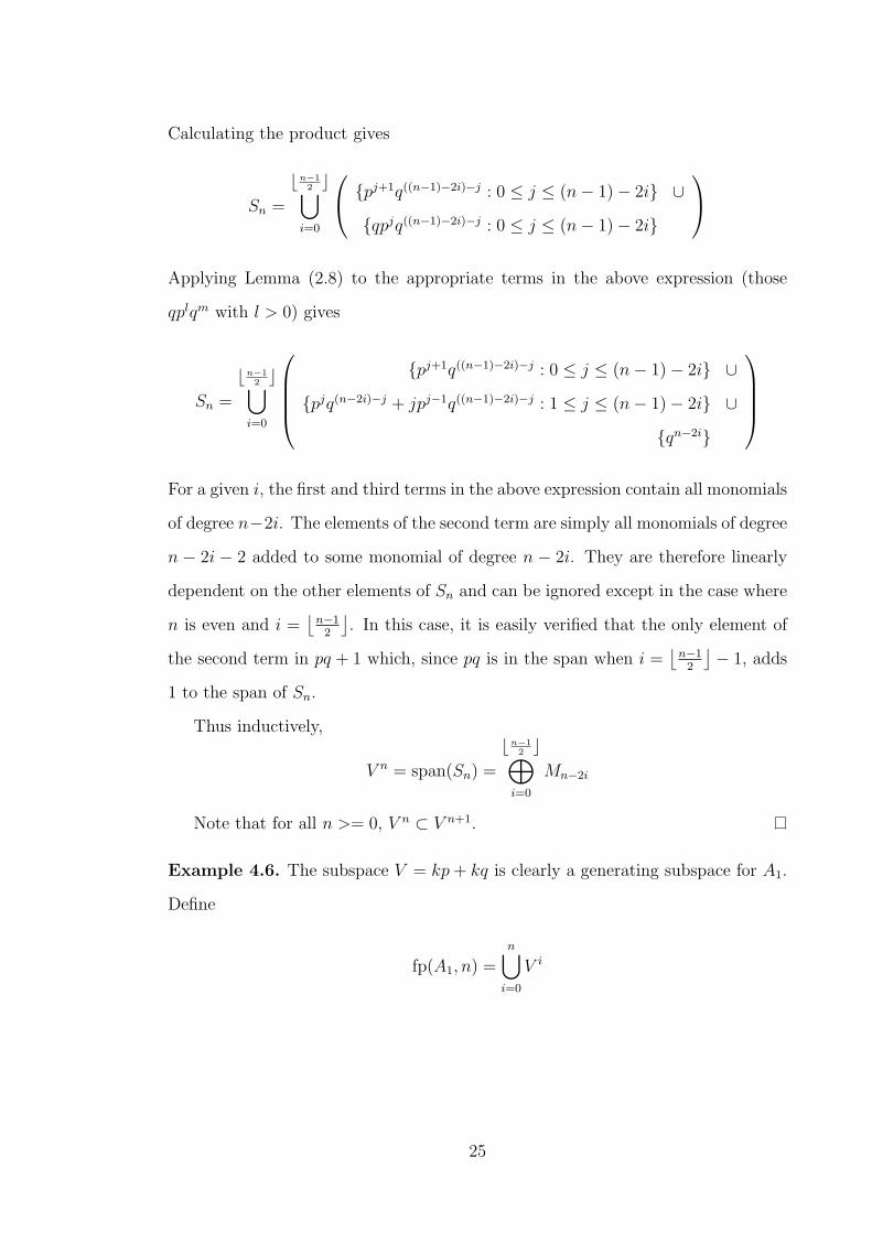
Calculating the product gives

Sn =

bn−12 c⋃

i=0

{pj+1q((n−1)−2i)−j : 0 ≤ j ≤ (n− 1)− 2i} ∪

{qpjq((n−1)−2i)−j : 0 ≤ j ≤ (n− 1)− 2i}

Applying Lemma (2.8) to the appropriate terms in the above expression (those

qplqm with l > 0) gives

Sn =

bn−12 c⋃

i=0

{pj+1q((n−1)−2i)−j : 0 ≤ j ≤ (n− 1)− 2i} ∪

{pjq(n−2i)−j + jpj−1q((n−1)−2i)−j : 1 ≤ j ≤ (n− 1)− 2i} ∪

{qn−2i}

For a given i, the first and third terms in the above expression contain all monomials

of degree n−2i. The elements of the second term are simply all monomials of degree

n − 2i − 2 added to some monomial of degree n − 2i. They are therefore linearly

dependent on the other elements of Sn and can be ignored except in the case where

n is even and i =⌊

n−12

⌋. In this case, it is easily verified that the only element of

the second term in pq + 1 which, since pq is in the span when i =⌊

n−12

⌋− 1, adds

1 to the span of Sn.

Thus inductively,

V n = span(Sn) =

bn−12 c⊕

i=0

Mn−2i

Note that for all n >= 0, V n ⊂ V n+1.

Example 4.6. The subspace V = kp+ kq is clearly a generating subspace for A1.

Define

fp(A1, n) =n⋃

i=0

V i

25

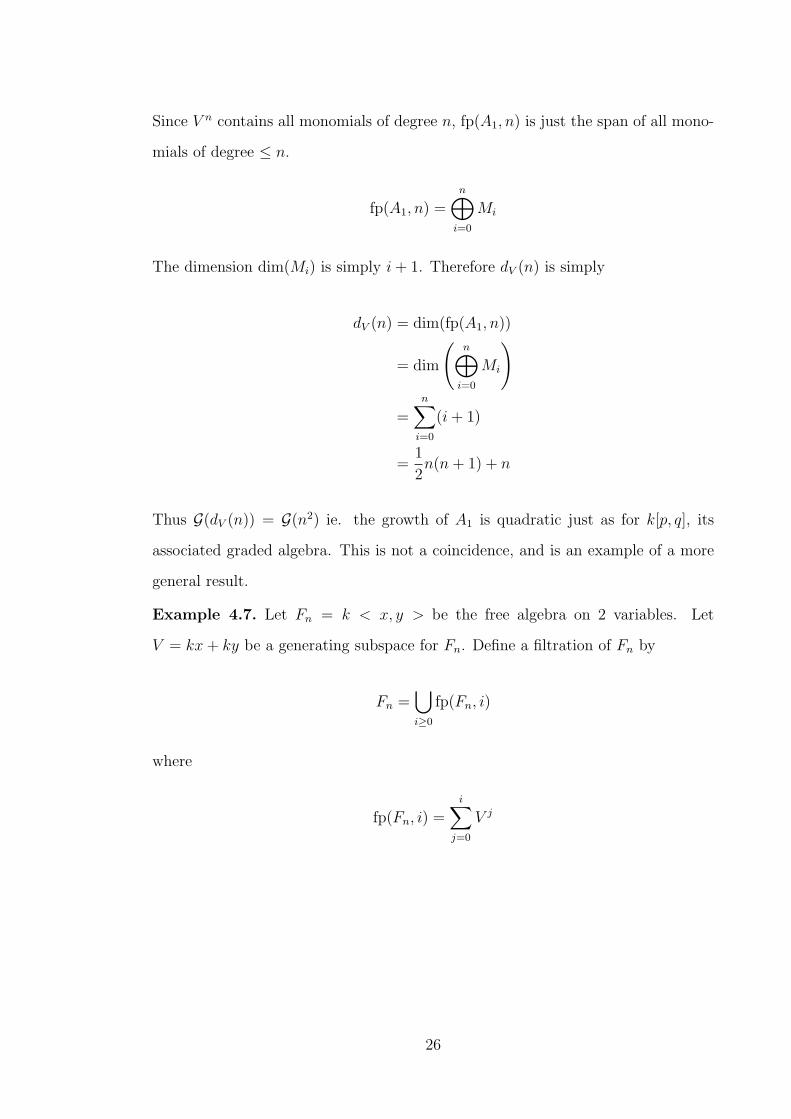
Since V n contains all monomials of degree n, fp(A1, n) is just the span of all mono-

mials of degree ≤ n.

fp(A1, n) =n⊕

i=0

Mi

The dimension dim(Mi) is simply i+ 1. Therefore dV (n) is simply

dV (n) = dim(fp(A1, n))

= dim

(n⊕

i=0

Mi

)

=n∑

i=0

(i+ 1)

=1

2n(n+ 1) + n

Thus G(dV (n)) = G(n2) ie. the growth of A1 is quadratic just as for k[p, q], its

associated graded algebra. This is not a coincidence, and is an example of a more

general result.

Example 4.7. Let Fn = k < x, y > be the free algebra on 2 variables. Let

V = kx+ ky be a generating subspace for Fn. Define a filtration of Fn by

Fn =⋃i≥0

fp(Fn, i)

where

fp(Fn, i) =i∑

j=0

V j

26

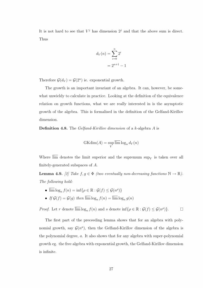
It is not hard to see that V j has dimension 2j and that the above sum is direct.

Thus

dV (n) =n∑

i=0

2i

= 2n+1 − 1

Therefore G(dV ) = G(2n) ie. exponential growth.

The growth is an important invariant of an algebra. It can, however, be some-

what unwieldy to calculate in practice. Looking at the definition of the equivalence

relation on growth functions, what we are really interested in is the asymptotic

growth of the algebra. This is formalised in the definition of the Gelfand-Kirillov

dimension.

Definition 4.8. The Gelfand-Kirillov dimension of a k-algebra A is

GKdim(A) = supV

lim logn dV (n)

Where lim denotes the limit superior and the supremum supV is taken over all

finitely-generated subspaces of A.

Lemma 4.9. [2] Take f, g ∈ Φ (two eventually non-decreasing functions N → R).

The following hold:

• lim logn f(n) = inf{ρ ∈ R : G(f) ≤ G(nρ)}

• If G(f) = G(g) then lim logn f(n) = lim logn g(n)

Proof. Let r denote lim logn f(n) and s denote inf{ρ ∈ R : G(f) ≤ G(nρ)}.

The first part of the preceeding lemma shows that for an algebra with poly-

nomial growth, say G(na), then the Gelfand-Kirillov dimension of the algebra is

the polynomial degree, a. It also shows that for any algebra with super-polynomial

growth eg. the free algebra with exponential growth, the Gelfand-Kirillov dimension

is infinite.

27

Note that in a previous lemma, we showed that for two generating subspaces V

and W , G(dV (n)) = G(dW (n)). Thus for any generating subspace V , we can drop

the supremum and write

GKdim(A) = lim logn dV (n)

The previous lemma also shows that the Gelfand-Kirillov dimension gives an

equivalence which is no finer than that given by the growth.

Remark. It has been proven (see [2] Chapter 2) that the range of possible values

for the Gelfand-Kirillov dimension of an algebra is {0} ∪ {1} ∪ [2,∞).

Remark. The Gelfand-Kirillov dimension can also be defined in a natural way for

modules over an algebra. The study of modules over the Weyl algebras is a par-

ticularly interesting application. It turns out that the minimum Gelfand-Kirillov

dimension for a module over the nth Weyl algebra An is 2n. Modules of this minimal

dimension are known as holonomic modules and are linked with holonomic systems

of linear differential equations.

Proposition 4.10. If A is an almost-commutative algebra with associated graded

algebra gr(A) then GKdim(A) = GKdim(gr(A)).

Proof. See [2] proposition 6.6.

28

Chapter 5

Automorphisms of A1

In this chapter, we show that all automorphisms of the first Weyl algebra, A1, are

generated by a set of automorphisms Φn,λ,Φ′n,λ which are defined shortly. This

proof originally appears in the paper [1] by Dixmier.

At this point, we need to define a number of concepts which are used in the

argument that follows.

Definition 5.1. If f =∑aijx

iyj ∈ k[x, y], denote by E(f) the set of pairs (i, j)

such that aij 6= 0. If ρ, σ are real numbers, define

vρ,σ(f) = sup(i,j)∈E(f)

(ρi+ σj)

(for convenience define vρ,σ(0) = −∞). Denote by E(f, ρ, σ) the set of pairs (i, j) ∈

E(f) such that ρi + σj = vρ,σ(f). If f 6= 0, we have E(f, ρ, σ) 6= ∅. If E(f) =

E(f, ρ, σ), we say that f is (ρ, σ)-homogeneous of (ρ, σ)-degree vρ,σ(f).

Remark. The above gives a grading of k[x, y] by (ρ, σ)-degree. This fact is not

required and the proof is omitted, but it does demonstrate the fact that there exist

more general gradings than those considered earlier.

Definition 5.2. Suppose a =∑aijp

iqj ∈ A1, and σ, ρ are real numbers. By

analogy with the previous definition (5.1), define E(a), vρ,σ(a) and E(a, ρ, σ). The

polynomial

∑(i,j)∈E(a,ρ,σ)

aijxiyj ∈ k[x, y]

29

is called the (ρ, σ)-associated polynomial of a.

Remark. The previous definition is an example of an associated graded algebra of

A1 corresponding to a more general filtration than that previously considered.

Lemma 5.3. Let f ∈ k[x, y] be a (ρ, σ)-homogeneous polynomial of (ρ, σ)-degree v.

Then,

• ρx δfδx

+ σy δfδy

= vf .

• If ρ and σ are linearly independent over Q, f is a monomial.

Proof. Let g = xiyj with ρi+ σj = v. We have

ρxδg

δx+ σy

δg

δy= ρxixi−1yj + σyjxiyj−1

= (ρi+ σj)g

and hence the first result.

If (i, j) ∈ E(f) and (i′, j′) ∈ E(f), we have ρi + σj = ρi′ + σj′ = v, thus

ρ(i − i′) = σ(j′ − j). Since ρ and σ are linearly independent, we must have i = i′

and j = j′, whence f is a monomial.

Lemma 5.4. Let f, g ∈ k[x, y] be (ρ, σ)-homogeneous polynomials of (ρ, σ) degrees

v, w. Then the following hold,

1.

σy

(δf

δx

δg

δy− δf

δy

δg

δx

)= wg

δf

δx− vf

δg

δx

Moreover, if both v and w are integers,

σy

(δf

δx

δg

δy− δf

δy

δg

δx

)= f−w+1gv+1 δ

δx(g−vfw)

30

2.

−ρx(δf

δx

δg

δy− δf

δy

δg

δx

)= wg

δf

δy− vf

δg

δy

Moreover, if both v and w are integers,

−ρx(δf

δx

δg

δy− δf

δy

δg

δx

)= f−w+1gv+1 δ

δy(g−vfw)

Proof. Applying lemma 5.3 part 1,

σy

(δf

δx

δg

δy− δf

δy

δg

δx

)=δf

δx

(wg − ρx

δg

δx

)−(vf − ρx

δf

δx

)δg

δx

= wgδf

δx− vf

δg

δx

Suppose that v and w are integers. Then

δ

δx(g−vfw) = g−v−1fw−1

(−v δg

δxf + gw

δf

δx

)

thus, taking into account the preceeding,

σy

(δf

δx

δg

δy− δf

δy

δg

δx

)= f−w+1gv+1 δ

δx(g−vfw)

Lemma 5.5. Take i, j, l,m integers ≥ 0. Then

(piqj)(plqm) = pi+lqj+m + jlpi+l−1qj+m−1 +1

2!j(j − 1)l(l − 1)pi+l−2qj+m−2

+1

3!j(j − 1)(j − 2)l(l − 1)(l − 2)pi+l−3qj+m−3 + . . .

Proof. This follows by expanding the expression derived in 2.9.

31

Lemma 5.6. Take a, b, c ∈ A1 with c = ab. Suppose

a =∑

aijpiqj b =

∑bijp

iqj c =∑

cijpiqj

Let

f =∑

aijxiyj g =

∑bijx

iyj h =∑

cijxiyj

Then

h = fg +δf

δy

δg

δx+

1

2!

δ2f

δy2

δ2g

δx2+

1

3!

δ3f

δy3

δ3g

δx3+ . . .

Proof. It suffices to prove for a = piqj, b = plqm, which follows from lemma 5.5.

Lemma 5.7. Take a, b, c ∈ A1 such that c = [a, b]. Suppose

a =∑

aijpiqj b =

∑bijp

iqj c =∑

cijpiqj

and let

f =∑

aijxiyj g =

∑bijx

iyj h =∑

cijxiyj

then

h =δf

δx

δg

δy− δf

δy

δg

δx+

1

2!

(δ2f

δx2

δ2g

δy2− δ2f

δy2

δ2g

δx2

)+

1

3!

(δ3f

δx3

δ3g

δy3− δ3f

δy3

δ3g

δx3

)+ . . .

Proof. This follows directly from lemma 5.6

Lemma 5.8. Take a and b non-zero elements of A1, and ρ, σ real numbers such that

ρ + σ > 0. Let v = vρ,σ(a) and w = vρ,σ(b). Let f1 and g1 be the (ρ, σ)-associated

polynomials of a and b.

(i) There exists a pair (t, u) of elements of A1, possessing the following properties:

(a) [x, y] = t+ u

32

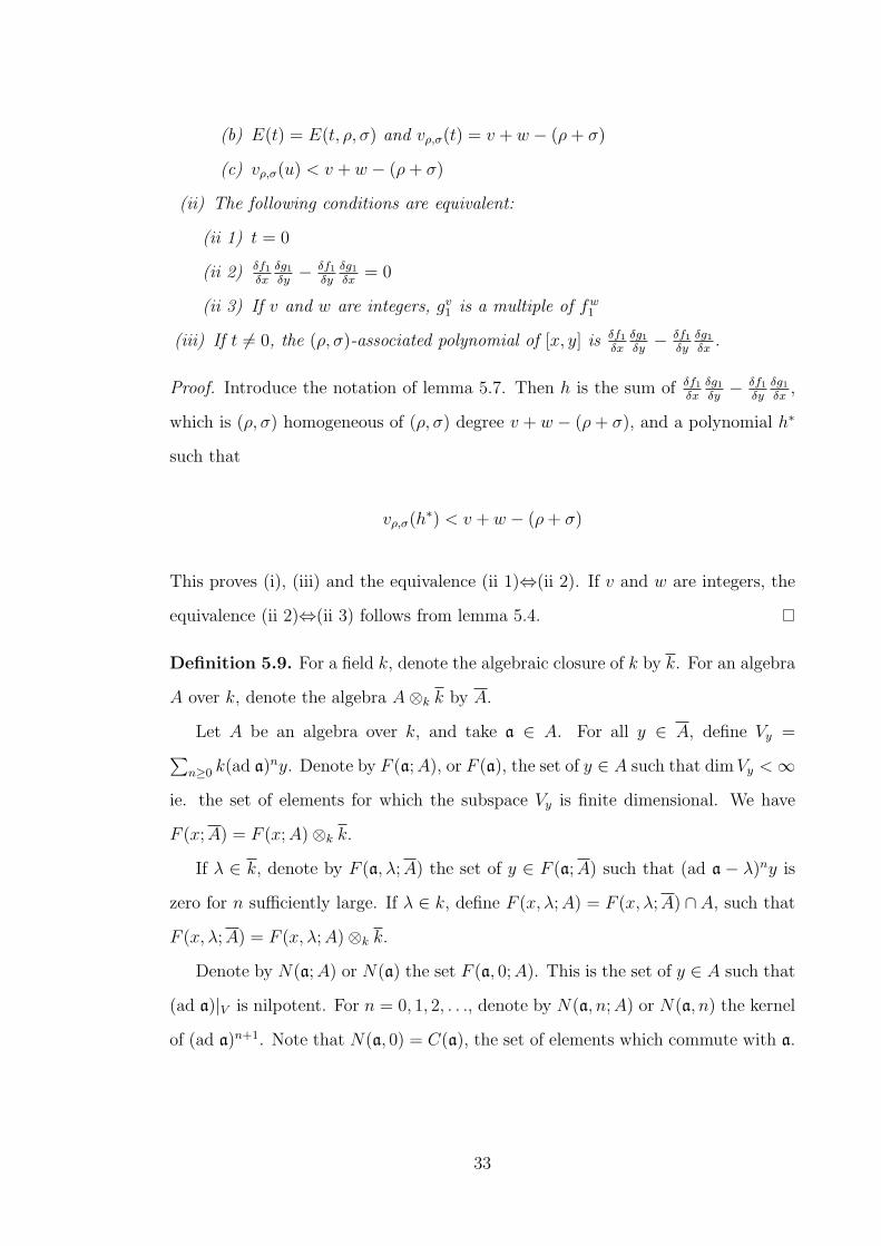
(b) E(t) = E(t, ρ, σ) and vρ,σ(t) = v + w − (ρ+ σ)

(c) vρ,σ(u) < v + w − (ρ+ σ)

(ii) The following conditions are equivalent:

(ii 1) t = 0

(ii 2) δf1

δxδg1

δy− δf1

δyδg1

δx= 0

(ii 3) If v and w are integers, gv1 is a multiple of fw

1

(iii) If t 6= 0, the (ρ, σ)-associated polynomial of [x, y] is δf1

δxδg1

δy− δf1

δyδg1

δx.

Proof. Introduce the notation of lemma 5.7. Then h is the sum of δf1

δxδg1

δy− δf1

δyδg1

δx,

which is (ρ, σ) homogeneous of (ρ, σ) degree v + w − (ρ+ σ), and a polynomial h∗

such that

vρ,σ(h∗) < v + w − (ρ+ σ)

This proves (i), (iii) and the equivalence (ii 1)⇔(ii 2). If v and w are integers, the

equivalence (ii 2)⇔(ii 3) follows from lemma 5.4.

Definition 5.9. For a field k, denote the algebraic closure of k by k. For an algebra

A over k, denote the algebra A⊗k k by A.

Let A be an algebra over k, and take a ∈ A. For all y ∈ A, define Vy =∑n≥0 k(ad a)ny. Denote by F (a;A), or F (a), the set of y ∈ A such that dimVy <∞

ie. the set of elements for which the subspace Vy is finite dimensional. We have

F (x;A) = F (x;A)⊗k k.

If λ ∈ k, denote by F (a, λ;A) the set of y ∈ F (a;A) such that (ad a − λ)ny is

zero for n sufficiently large. If λ ∈ k, define F (x, λ;A) = F (x, λ;A) ∩ A, such that

F (x, λ;A) = F (x, λ;A)⊗k k.

Denote by N(a;A) or N(a) the set F (a, 0;A). This is the set of y ∈ A such that

(ad a)|V is nilpotent. For n = 0, 1, 2, . . ., denote by N(a, n;A) or N(a, n) the kernel

of (ad a)n+1. Note that N(a, 0) = C(a), the set of elements which commute with a.

33

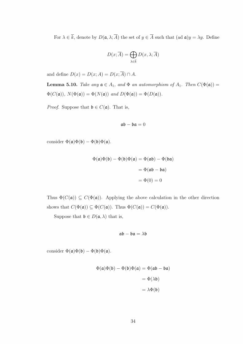
For λ ∈ k, denote by D(a, λ;A) the set of y ∈ A such that (ad a)y = λy. Define

D(x;A) =⊕λ∈k

D(x, λ;A)

and define D(x) = D(x;A) = D(x;A) ∩ A.

Lemma 5.10. Take any a ∈ A1, and Φ an automorphism of A1. Then C(Φ(a)) =

Φ(C(a)), N(Φ(a)) = Φ(N(a)) and D(Φ(a)) = Φ(D(a)).

Proof. Suppose that b ∈ C(a). That is,

ab− ba = 0

consider Φ(a)Φ(b)− Φ(b)Φ(a).

Φ(a)Φ(b)− Φ(b)Φ(a) = Φ(ab)− Φ(ba)

= Φ(ab− ba)

= Φ(0) = 0

Thus Φ(C(a)) ⊆ C(Φ(a)). Applying the above calculation in the other direction

shows that C(Φ(a)) ⊆ Φ(C(a)). Thus Φ(C(a)) = C(Φ(a)).

Suppose that b ∈ D(a, λ) that is,

ab− ba = λb

consider Φ(a)Φ(b)− Φ(b)Φ(a).

Φ(a)Φ(b)− Φ(b)Φ(a) = Φ(ab− ba)

= Φ(λb)

= λΦ(b)

34

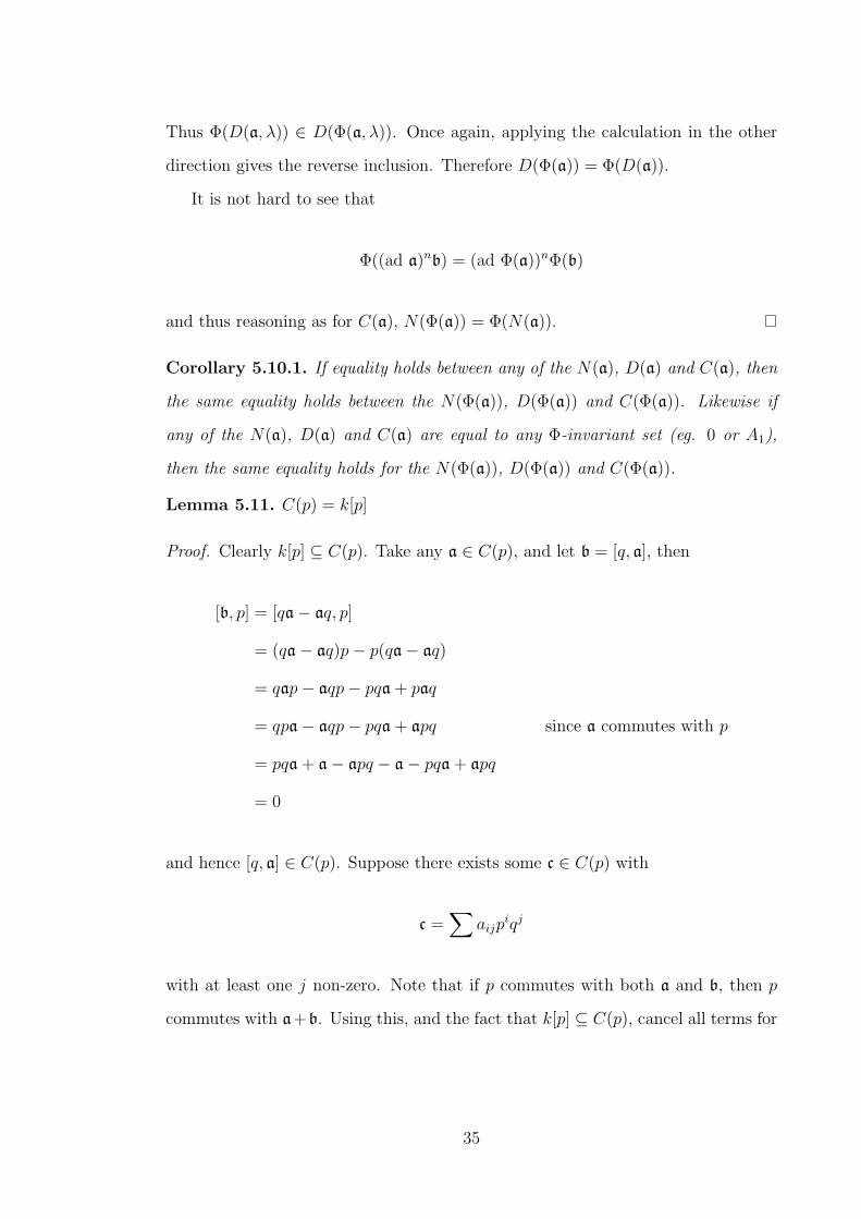
Thus Φ(D(a, λ)) ∈ D(Φ(a, λ)). Once again, applying the calculation in the other

direction gives the reverse inclusion. Therefore D(Φ(a)) = Φ(D(a)).

It is not hard to see that

Φ((ad a)nb) = (ad Φ(a))nΦ(b)

and thus reasoning as for C(a), N(Φ(a)) = Φ(N(a)).

Corollary 5.10.1. If equality holds between any of the N(a), D(a) and C(a), then

the same equality holds between the N(Φ(a)), D(Φ(a)) and C(Φ(a)). Likewise if

any of the N(a), D(a) and C(a) are equal to any Φ-invariant set (eg. 0 or A1),

then the same equality holds for the N(Φ(a)), D(Φ(a)) and C(Φ(a)).

Lemma 5.11. C(p) = k[p]

Proof. Clearly k[p] ⊆ C(p). Take any a ∈ C(p), and let b = [q, a], then

[b, p] = [qa− aq, p]

= (qa− aq)p− p(qa− aq)

= qap− aqp− pqa + paq

= qpa− aqp− pqa + apq since a commutes with p

= pqa + a− apq − a− pqa + apq

= 0

and hence [q, a] ∈ C(p). Suppose there exists some c ∈ C(p) with

c =∑

aijpiqj

with at least one j non-zero. Note that if p commutes with both a and b, then p

commutes with a+b. Using this, and the fact that k[p] ⊆ C(p), cancel all terms for

35

which j = 0 to get some c′ ∈ C(p) for which every term contains a positive power

of q. Calculate [q, c′]:

[q, c′] = qc′ − c′q

=∑

aij(qpiqj − piqj+1) since [−,−] is bilinear

=∑

aij(piqj+1 + ipi−1qj − piqj+1) by lemma 2.8

=∑

aijipi−1qj

Note that we have decreased the degree in p by one in each term, and every term

for which i = 0 becomes zero. Pick i0 to be maximal with respect to the property

that ai0,j is non-zero for some j. And apply the above operation i0 times to get

another element c′′ ∈ C(p). By the choice of i0,

c′′ =∑

j

ai0jqj

since terms with a lower power of p will vanish (note that the terms of this sum

are not neccessarily unique). Equating coefficients of [p, c′′] implies that [p, qj] = 0,

which is a contradiction. Therefore c /∈ C(p) and C(p) = k[p].

Lemma 5.12. Let A be an algebra over k. Take λ ∈ k and a, b ∈ A such that

(ad a− λ)2b = 0. Then

1. (ad a− nλ)nbn = n!((ad a− λ)b)n for n = 1, 2, 3, . . .

2. (ad a− nλ)n+1bn = 0

Proof. The assumption (ad a− λ)2b = 0 can be written as

(ad a− λ)b ∈ D(a, λ)

Since D(a, λ;A).D(a, µ;A) ⊂ D(a, λ+ µ;A),

((ad a− λ)b)n ∈ D(a, nλ) for n = 1, 2, 3, . . . (5.1)

36

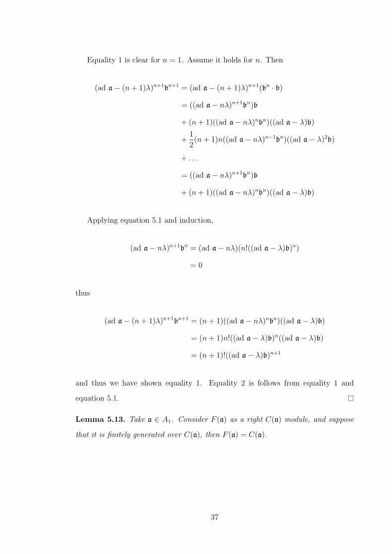
Equality 1 is clear for n = 1. Assume it holds for n. Then

(ad a− (n+ 1)λ)n+1bn+1 = (ad a− (n+ 1)λ)n+1(bn · b)

= ((ad a− nλ)n+1bn)b

+ (n+ 1)((ad a− nλ)nbn)((ad a− λ)b)

+1

2(n+ 1)n((ad a− nλ)n−1bn)((ad a− λ)2b)

+ . . .

= ((ad a− nλ)n+1bn)b

+ (n+ 1)((ad a− nλ)nbn)((ad a− λ)b)

Applying equation 5.1 and induction,

(ad a− nλ)n+1bn = (ad a− nλ)(n!((ad a− λ)b)n)

= 0

thus

(ad a− (n+ 1)λ)n+1bn+1 = (n+ 1)((ad a− nλ)nbn)((ad a− λ)b)

= (n+ 1)n!((ad a− λ)b)n((ad a− λ)b)

= (n+ 1)!((ad a− λ)b)n+1

and thus we have shown equality 1. Equality 2 is follows from equality 1 and

equation 5.1.

Lemma 5.13. Take a ∈ A1. Consider F (a) as a right C(a) module, and suppose

that it is finitely generated over C(a), then F (a) = C(a).

37

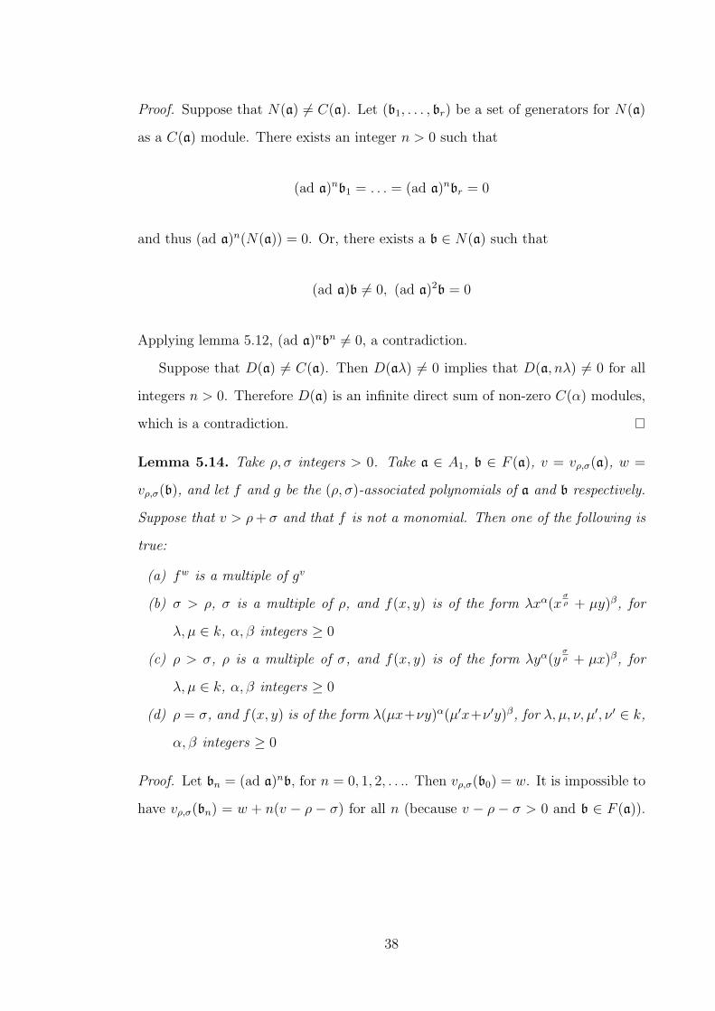
Proof. Suppose that N(a) 6= C(a). Let (b1, . . . , br) be a set of generators for N(a)

as a C(a) module. There exists an integer n > 0 such that

(ad a)nb1 = . . . = (ad a)nbr = 0

and thus (ad a)n(N(a)) = 0. Or, there exists a b ∈ N(a) such that

(ad a)b 6= 0, (ad a)2b = 0

Applying lemma 5.12, (ad a)nbn 6= 0, a contradiction.

Suppose that D(a) 6= C(a). Then D(aλ) 6= 0 implies that D(a, nλ) 6= 0 for all

integers n > 0. Therefore D(a) is an infinite direct sum of non-zero C(α) modules,

which is a contradiction.

Lemma 5.14. Take ρ, σ integers > 0. Take a ∈ A1, b ∈ F (a), v = vρ,σ(a), w =

vρ,σ(b), and let f and g be the (ρ, σ)-associated polynomials of a and b respectively.

Suppose that v > ρ+ σ and that f is not a monomial. Then one of the following is

true:

(a) fw is a multiple of gv

(b) σ > ρ, σ is a multiple of ρ, and f(x, y) is of the form λxα(xσρ + µy)β, for

λ, µ ∈ k, α, β integers ≥ 0

(c) ρ > σ, ρ is a multiple of σ, and f(x, y) is of the form λyα(yσρ + µx)β, for

λ, µ ∈ k, α, β integers ≥ 0

(d) ρ = σ, and f(x, y) is of the form λ(µx+νy)α(µ′x+ν ′y)β, for λ, µ, ν, µ′, ν ′ ∈ k,

α, β integers ≥ 0

Proof. Let bn = (ad a)nb, for n = 0, 1, 2, . . .. Then vρ,σ(b0) = w. It is impossible to

have vρ,σ(bn) = w + n(v − ρ − σ) for all n (because v − ρ − σ > 0 and b ∈ F (a)).

38

Thus there exists an n ≥ 0 such that

vρ,σ(bm) = w +m(v − ρ+ σ) for m ≤ n and

vρ,σ(bn+1) < w + (n+ 1)(v − ρ− σ)

Let h be the (ρ, σ)-associated polynomial of bn. Let vρ,σ(bn) = t. Applying

lemma 5.8, f t is a multiple of hv. If n = 0, we have bn = b, h = g and t = w

ie. case (a). Suppose from now on that n > 0. Consider bn−1. Let l be the

(ρ, σ)-associated polynomial of bn−1. We have vρ,σ(bn) − vρ,σ(bn−1) = v − ρ − σ,

thus

vρ,σ(bn−1) = t− v + ρ+ σ

Thus

σyh = σy

(δf

δx

δl

δy− δf

δy

δl

δx

)lemma 5.8 part 3

= f−t+v−ρ−σ+1lv+1 δ

δx(l−vf l−v+ρ+σ) lemma 5.4 part 1

thus, since f t is a multiple of hv,

δ

δx

((h

fl

)v

fρ+σ

)= σy

(h

fl

)v+1

fρ+σ (5.2)

By utilising lemma 5.4 part 2 instead of part 1, it follows similarly that

δ

δy

((h

fl

)v

fρ+σ

)= −ρx

(h

fl

)v+1

fρ+σ (5.3)

Consider f ,h and l as polynomials in x with coefficients in k(y). Take µ ∈ k(y).

If µ is a zero of hfl

of order ν > 0 and a zero of f of order ν ′ ≥ 0, the relation 5.2

shows that vν + (ρ + σ)ν ′ − 1 = (v + 1)ν + (ρ + σ)ν ′, which is impossible. Thus

hdl

is non-zero on k(y). Therefore, flh∈ k(y)[x]. Applying 5.3, we see similarly

39

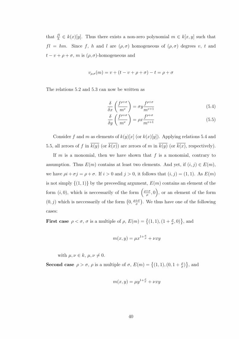
that flh∈ k(x)[y]. Thus there exists a non-zero polynomial m ∈ k[x, y] such that

fl = hm. Since f , h and l are (ρ, σ) homogeneous of (ρ, σ) degrees v, t and

t− v + ρ+ σ, m is (ρ, σ)-homogeneous and

vρ,σ(m) = v + (t− v + ρ+ σ)− t = ρ+ σ

The relations 5.2 and 5.3 can now be written as

δ

δx

(fρ+σ

mv

)= σy

fρ+σ

mv+1(5.4)

δ

δy

(fρ+σ

mv

)= ρx

fρ+σ

mv+1(5.5)

Consider f and m as elements of k(y)[x] (or k(x)[y]). Applying relations 5.4 and

5.5, all zeroes of f in k(y) (or k(x)) are zeroes of m in k(y) (or k(x), respectively).

If m is a monomial, then we have shown that f is a monomial, contrary to

assumption. Thus E(m) contains at least two elements. And yet, if (i, j) ∈ E(m),

we have ρi+ σj = ρ+ σ. If i > 0 and j > 0, it follows that (i, j) = (1, 1). As E(m)

is not simply {(1, 1)} by the preceeding argument, E(m) contains an element of the

form (i, 0), which is neccessarily of the form(

ρ+σρ, 0), or an element of the form

(0, j) which is neccessarily of the form(0, ρ+σ

σ

). We thus have one of the following

cases:

First case ρ < σ, σ is a multiple of ρ, E(m) ={(1, 1), (1 + ρ

σ, 0)}, and

m(x, y) = µx1+σρ + νxy

with µ, ν ∈ k, µ, ν 6= 0.

Second case ρ > σ, ρ is a multiple of σ, E(m) ={(1, 1), (0, 1 + ρ

σ)}, and

m(x, y) = µy1+ ρσ + νxy

40

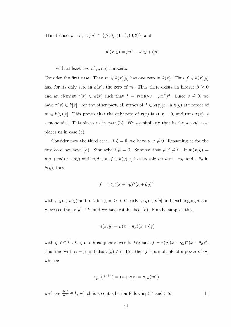
Third case ρ = σ, E(m) ⊂ {(2, 0), (1, 1), (0, 2)}, and

m(x, y) = µx2 + νxy + ζy2

with at least two of µ, ν, ζ non-zero.

Consider the first case. Then m ∈ k(x)[y] has one zero in k(x). Thus f ∈ k(x)[y]

has, for its only zero in k(x), the zero of m. Thus there exists an integer β ≥ 0

and an element τ(x) ∈ k(x) such that f = τ(x)(νy + µxσρ )β. Since v 6= 0, we

have τ(x) ∈ k[x]. For the other part, all zeroes of f ∈ k(y)[x] in k(y) are zeroes of

m ∈ k(y)[x]. This proves that the only zero of τ(x) is at x = 0, and thus τ(x) is

a monomial. This places us in case (b). We see similarly that in the second case

places us in case (c).

Consider now the third case. If ζ = 0, we have µ, ν 6= 0. Reasoning as for the

first case, we have (d). Similarly if µ = 0. Suppose that µ, ζ 6= 0. If m(x, y) =

µ(x + ηy)(x + θy) with η, θ ∈ k, f ∈ k(y)[x] has its sole zeros at −ηy, and −θy in

k(y), thus

f = τ(y)(x+ ηy)α(x+ θy)β

with τ(y) ∈ k(y) and α, β integers ≥ 0. Clearly, τ(y) ∈ k[y] and, exchanging x and

y, we see that τ(y) ∈ k, and we have established (d). Finally, suppose that

m(x, y) = µ(x+ ηy)(x+ θy)

with η, θ ∈ k \ k, η and θ conjugate over k. We have f = τ(y)(x + ηy)α(x + θy)β,

this time with α = β and also τ(y) ∈ k. But then f is a multiple of a power of m,

whence

vρ,σ(fρ+σ) = (ρ+ σ)v = vρ,σ(mv)

we have fρ,σ

mv ∈ k, which is a contradiction following 5.4 and 5.5.

41

Proposition 5.15. Take ρ, σ integers > 0, a ∈ A1, v = vρ,σ(a), let f be the (ρ, σ)-

associated polynomial of a. Suppose that

1. v > ρ+ σ

2. f is not a monomial

3. None of the cases (b), (c), or (d) in lemma 5.14 hold

Then F (a) = C(a).

Proof. Let Λ be the set of integers λ for which there exists a b ∈ F (a) with vρ,σ(b) =

λ. Since F (a) is closed under addition, Λ+Λ ⊂ Λ, and in particular {0, v, 2v, . . .} ⊂

Λ. Let Λ′ be the image in N/vN of Λ under the map n 7→ n + vN. In every

(coset) element of Λ′, choose the smallest element. Denote these elements by λ0 =

0, λ1, . . . , λr where r ≤ v. The elements of Λ are then of the following form:

0, v, 2v, 3v, . . .

λ1, λ1 + v, λ1 + 2v, λ1 + 3v, . . .

...

λr, λr + v, λr + 2v, λr + 3v, . . .

Let bi be an element of F (a) such that vρ,σ(bi) = λi. Take b ∈ F (a). We will

show by induction that b ∈ k[a]b0+k[a]b1+. . .+k[a]br. It is obvious for vρ,σ(b) = 0.

Suppose that it holds for vρ,σ(b) < n and consider the case where vρ,σ(b) = n > 0.

Then there exists an i ∈ {0, 1, . . . , r} and an integer s ≥ 0 such that vρ,σ(asbk) = n.

Let g and h be the (ρ, σ)-associated polynomials of b and asbi. Applying lemma

5.14, gv and hv are scalar multiples of fn and thus of each other. Thus there exists

a λ ∈ k such that vρ,σ(b−λasbi) < n. We have therefore b−λasbi ∈ F (a), and the

result follows by induction on b− λasbi.

Thus we have F (a) =∑

i k[a]bi and the result follows from lemma 5.13.

42

Definition 5.16. For λ ∈ k and n ∈ N, define the k-linear maps Φn,λ,Φ′n,λ : A1 →

A1 by

Φn,λ(p) = p Φn,λ(q) = q + λpn

Φ′n,λ(p) = p+ λqn Φ′

n,λ(q) = q

Lemma 5.17. For all λ ∈ k and n ∈ N, Φn,λ and Φ′n,λ are k-linear automorphisms

of A1.

Proof. The image of qp− pq − 1 under Φn,λ is

(q + λpn)p− p(q + λpn)− 1 = qp+ λpn+1 − pq − λpn+1 − 1

= pq + 1 + λpn+1 − pq − λpn+1 − 1

= 0

thus Φn,λ is an homomorphism. Similarly for Φ′n,λ. As mentioned at the end of

chapter 2, the fact that A1 is simple implies that any non-zero endomorphism of

A1 is injective. This follows as the kernel is an ideal of A1 and is therefore either

0 or all of A1. Thus both Φn,λ and Φ′n,λ are injective. Let q0 = −λpn + q and let

p0 = p− λqn. We have,

Φn,λ(p) = p Φn,λ(q0) = −λpn + q + λpn = q

Φ′n,λ(p0) = p+ λqn − λqn = p Φ′

n,λ(q) = q

Thus p and q are in the images of both Φn,λ and Φ′n,λ and they are thus both

surjective.

Definition 5.18. Let G denote the group of automorphisms of A1 generated by

the Φn,λ,Φ′n,λ for all n, λ.

43

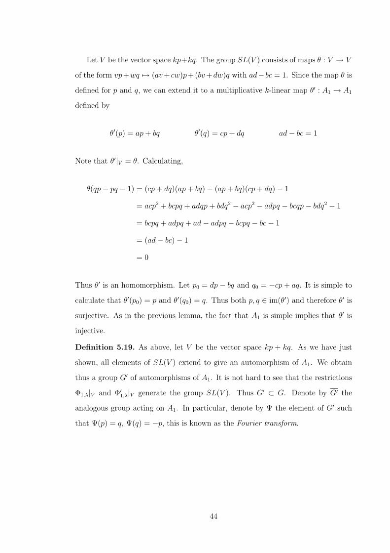
Let V be the vector space kp+kq. The group SL(V ) consists of maps θ : V → V

of the form vp+wq 7→ (av+ cw)p+(bv+dw)q with ad− bc = 1. Since the map θ is

defined for p and q, we can extend it to a multiplicative k-linear map θ′ : A1 → A1

defined by

θ′(p) = ap+ bq θ′(q) = cp+ dq ad− bc = 1

Note that θ′|V = θ. Calculating,

θ(qp− pq − 1) = (cp+ dq)(ap+ bq)− (ap+ bq)(cp+ dq)− 1

= acp2 + bcpq + adqp+ bdq2 − acp2 − adpq − bcqp− bdq2 − 1

= bcpq + adpq + ad− adpq − bcpq − bc− 1

= (ad− bc)− 1

= 0

Thus θ′ is an homomorphism. Let p0 = dp− bq and q0 = −cp+ aq. It is simple to

calculate that θ′(p0) = p and θ′(q0) = q. Thus both p, q ∈ im(θ′) and therefore θ′ is

surjective. As in the previous lemma, the fact that A1 is simple implies that θ′ is

injective.

Definition 5.19. As above, let V be the vector space kp + kq. As we have just

shown, all elements of SL(V ) extend to give an automorphism of A1. We obtain

thus a group G′ of automorphisms of A1. It is not hard to see that the restrictions

Φ1,λ|V and Φ′1,λ|V generate the group SL(V ). Thus G′ ⊂ G. Denote by G′ the

analogous group acting on A1. In particular, denote by Ψ the element of G′ such

that Ψ(p) = q, Ψ(q) = −p, this is known as the Fourier transform.

44

Lemma 5.20. Take a = αp2 + βpq + γq2 ∈ A1 with α, β, γ ∈ k. There exist

Φ,Θ ∈ G′ such that

Φ(a) = θpq + ζ

Θ(a) =

α′p2 + ζ ′, if β2 − αγ = 0

α′p2 + γ′q2 + ζ ′, if β2 − αγ 6= 0

for α′, γ′, ζ ′ ∈ k and θ, ζ ∈ k.

Proof. Noting that if Φ(p) = ap+ bq and Φ(q) = cp+ dq,

Φ(a) = α(ap+ bq)2 + β(ap+ bq)(cp+ dq) + γ(cp+ dq)2

= αa2p2 + αabpq + αabqp+ αb2q2

+ βacp2 + βadpq + βbcqp+ βbdq2

+ γc2p2 + γcdpq + γcdqp+ γd2q2

= (αa2 + βac+ γc2)p2 + (2αab+ βad+ βbc+ 2γcd)pq

+ (αb2 + βbd+ γd2)q2 + αab+ βbc+ γcd

which is simply the action of Φ|V on a considered as a quadratic form in k[p, q] plus

a scalar term. The result thus follows from the analogous results for real quadratic

forms on two variables.

Lemma 5.21. For a ∈ k[p], N(a) = A1.

Proof. First note that for b, c ∈ A1, if (ad a)mb = 0 and (ad a)nc = 0 then if

o = max(m,n), (ad a)o(b + c) = (ad a)ob + (ad a)oc = 0 and (ad a)o(bc) =

((ad a)ob)c + b((ad a)oc) = 0 ie. N(a) is both multiplicatively and additively

closed.

We have p ∈ N(a) and [a, q] ∈ k[p], whence q ∈ N(a) and thus A1 ⊆ N(a).

Lemma 5.22. Take a = λp2 + µq2 + ν with λ, µ, ν ∈ k, λ 6= 0, µ 6= 0. Then

D(a) = A1.

45

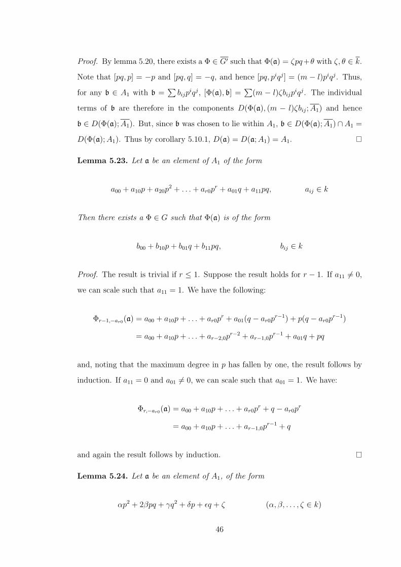
Proof. By lemma 5.20, there exists a Φ ∈ G′ such that Φ(a) = ζpq+θ with ζ, θ ∈ k.

Note that [pq, p] = −p and [pq, q] = −q, and hence [pq, piqj] = (m − l)piqj. Thus,

for any b ∈ A1 with b =∑bijp

iqj, [Φ(a), b] =∑

(m − l)ζbijpiqj. The individual

terms of b are therefore in the components D(Φ(a), (m − l)ζbij;A1) and hence

b ∈ D(Φ(a);A1). But, since b was chosen to lie within A1, b ∈ D(Φ(a);A1)∩A1 =

D(Φ(a);A1). Thus by corollary 5.10.1, D(a) = D(a;A1) = A1.

Lemma 5.23. Let a be an element of A1 of the form

a00 + a10p+ a20p2 + . . .+ ar0p

r + a01q + a11pq, aij ∈ k

Then there exists a Φ ∈ G such that Φ(a) is of the form

b00 + b10p+ b01q + b11pq, bij ∈ k

Proof. The result is trivial if r ≤ 1. Suppose the result holds for r − 1. If a11 6= 0,

we can scale such that a11 = 1. We have the following:

Φr−1,−ar0(a) = a00 + a10p+ . . .+ ar0pr + a01(q − ar0p

r−1) + p(q − ar0pr−1)

= a00 + a10p+ . . .+ ar−2,0pr−2 + ar−1,0p

r−1 + a01q + pq

and, noting that the maximum degree in p has fallen by one, the result follows by

induction. If a11 = 0 and a01 6= 0, we can scale such that a01 = 1. We have:

Φr,−ar0(a) = a00 + a10p+ . . .+ ar0pr + q − ar0p

r

= a00 + a10p+ . . .+ ar−1,0pr−1 + q

and again the result follows by induction.

Lemma 5.24. Let a be an element of A1, of the form

αp2 + 2βpq + γq2 + δp+ εq + ζ (α, β, . . . , ζ ∈ k)

46

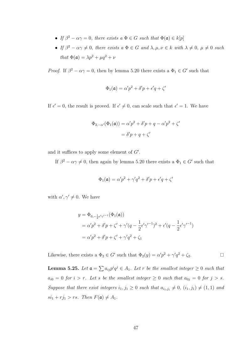
• If β2 − αγ = 0, there exists a Φ ∈ G such that Φ(a) ∈ k[p]

• If β2 − αγ 6= 0, there exists a Φ ∈ G and λ, µ, ν ∈ k with λ 6= 0, µ 6= 0 such

that Φ(a) = λp2 + µq2 + ν

Proof. If β2 − αγ = 0, then by lemma 5.20 there exists a Φ1 ∈ G′ such that

Φ1(a) = α′p2 + δ′p+ ε′q + ζ ′

If ε′ = 0, the result is proved. If ε′ 6= 0, can scale such that ε′ = 1. We have

Φ2,−α′(Φ1(a)) = α′p2 + δ′p+ q − α′p2 + ζ ′

= δ′p+ q + ζ ′

and it suffices to apply some element of G′.

If β2 − αγ 6= 0, then again by lemma 5.20 there exists a Φ1 ∈ G′ such that

Φ1(a) = α′p2 + γ′q2 + δ′p+ ε′q + ζ ′

with α′, γ′ 6= 0. We have

y = Φ0,− 12ε′γ′−1(Φ1(a))

= α′p2 + δ′p+ ζ ′ + γ′(q − 1

2ε′γ′

−1)2 + ε′(q − 1

2ε′γ′

−1)

= α′p2 + δ′p+ ζ ′ + γ′q2 + ζ1

Likewise, there exists a Φ2 ∈ G′ such that Φ2(y) = α′p2 + γ′q2 + ζ2.

Lemma 5.25. Let a =∑aijp

iqj ∈ A1. Let r be the smallest integer ≥ 0 such that

ai0 = 0 for i > r. Let s be the smallest integer ≥ 0 such that a0j = 0 for j > s.

Suppose that there exist integers i1, j1 ≥ 0 such that ai1,j1 6= 0, (i1, j1) 6= (1, 1) and

si1 + rj1 > rs. Then F (a) 6= A1.

47

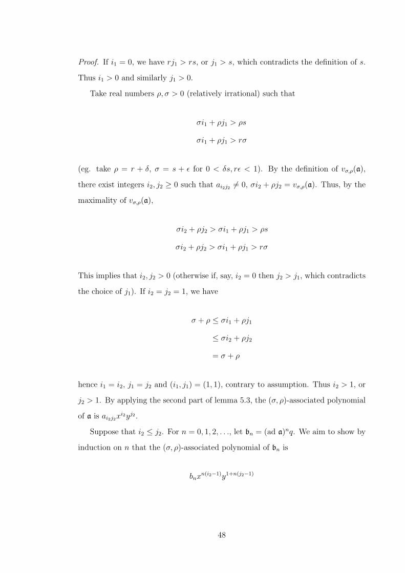
Proof. If i1 = 0, we have rj1 > rs, or j1 > s, which contradicts the definition of s.

Thus i1 > 0 and similarly j1 > 0.

Take real numbers ρ, σ > 0 (relatively irrational) such that

σi1 + ρj1 > ρs

σi1 + ρj1 > rσ

(eg. take ρ = r + δ, σ = s + ε for 0 < δs, rε < 1). By the definition of vσ,ρ(a),

there exist integers i2, j2 ≥ 0 such that ai2j2 6= 0, σi2 + ρj2 = vσ,ρ(a). Thus, by the

maximality of vσ,ρ(a),

σi2 + ρj2 > σi1 + ρj1 > ρs

σi2 + ρj2 > σi1 + ρj1 > rσ

This implies that i2, j2 > 0 (otherwise if, say, i2 = 0 then j2 > j1, which contradicts

the choice of j1). If i2 = j2 = 1, we have

σ + ρ ≤ σi1 + ρj1

≤ σi2 + ρj2

= σ + ρ

hence i1 = i2, j1 = j2 and (i1, j1) = (1, 1), contrary to assumption. Thus i2 > 1, or

j2 > 1. By applying the second part of lemma 5.3, the (σ, ρ)-associated polynomial

of a is ai2j2xi2yj2 .

Suppose that i2 ≤ j2. For n = 0, 1, 2, . . ., let bn = (ad a)nq. We aim to show by

induction on n that the (σ, ρ)-associated polynomial of bn is

bnxn(i2−1)y1+n(j2−1)

48

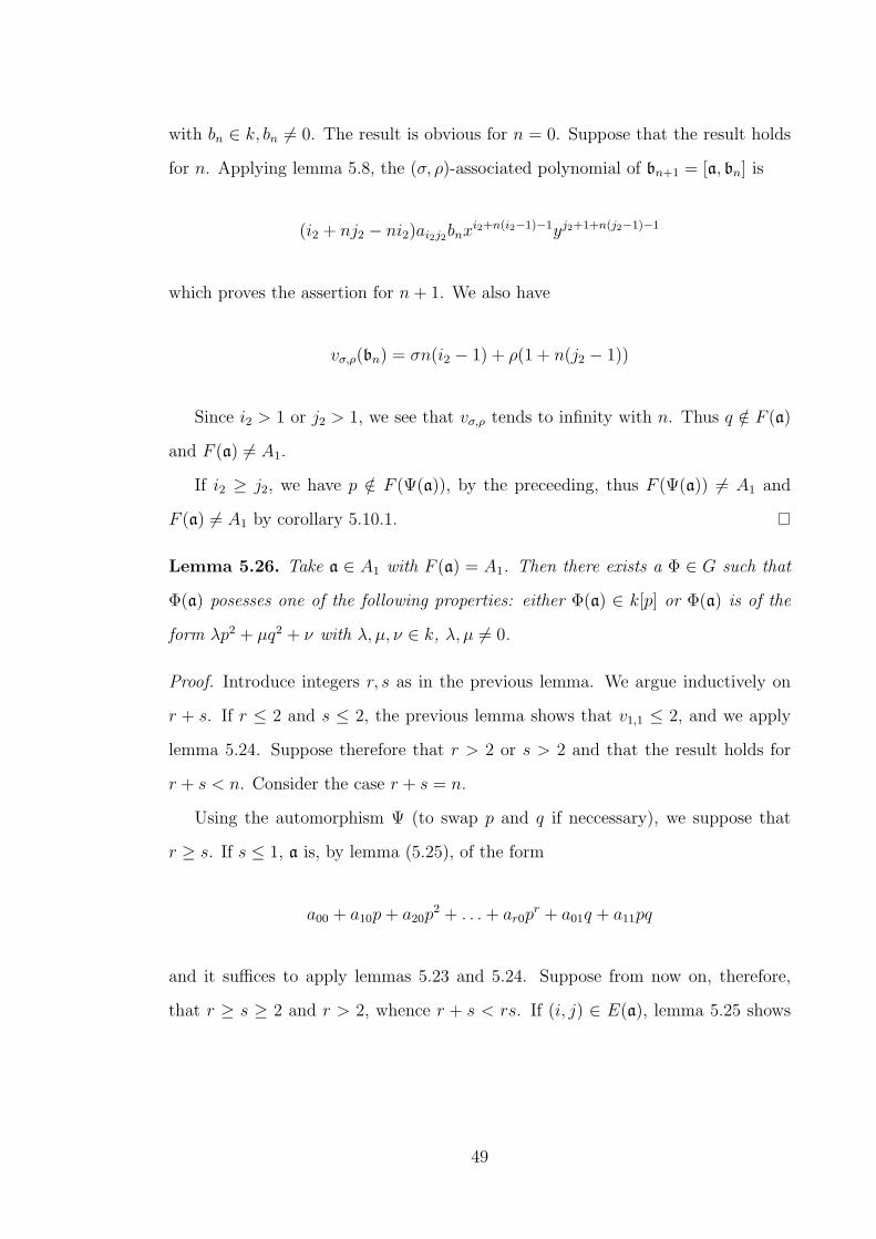
with bn ∈ k, bn 6= 0. The result is obvious for n = 0. Suppose that the result holds

for n. Applying lemma 5.8, the (σ, ρ)-associated polynomial of bn+1 = [a, bn] is

(i2 + nj2 − ni2)ai2j2bnxi2+n(i2−1)−1yj2+1+n(j2−1)−1

which proves the assertion for n+ 1. We also have

vσ,ρ(bn) = σn(i2 − 1) + ρ(1 + n(j2 − 1))

Since i2 > 1 or j2 > 1, we see that vσ,ρ tends to infinity with n. Thus q /∈ F (a)

and F (a) 6= A1.

If i2 ≥ j2, we have p /∈ F (Ψ(a)), by the preceeding, thus F (Ψ(a)) 6= A1 and

F (a) 6= A1 by corollary 5.10.1.

Lemma 5.26. Take a ∈ A1 with F (a) = A1. Then there exists a Φ ∈ G such that

Φ(a) posesses one of the following properties: either Φ(a) ∈ k[p] or Φ(a) is of the

form λp2 + µq2 + ν with λ, µ, ν ∈ k, λ, µ 6= 0.

Proof. Introduce integers r, s as in the previous lemma. We argue inductively on

r + s. If r ≤ 2 and s ≤ 2, the previous lemma shows that v1,1 ≤ 2, and we apply

lemma 5.24. Suppose therefore that r > 2 or s > 2 and that the result holds for

r + s < n. Consider the case r + s = n.

Using the automorphism Ψ (to swap p and q if neccessary), we suppose that

r ≥ s. If s ≤ 1, a is, by lemma (5.25), of the form

a00 + a10p+ a20p2 + . . .+ ar0p

r + a01q + a11pq

and it suffices to apply lemmas 5.23 and 5.24. Suppose from now on, therefore,

that r ≥ s ≥ 2 and r > 2, whence r + s < rs. If (i, j) ∈ E(a), lemma 5.25 shows

49

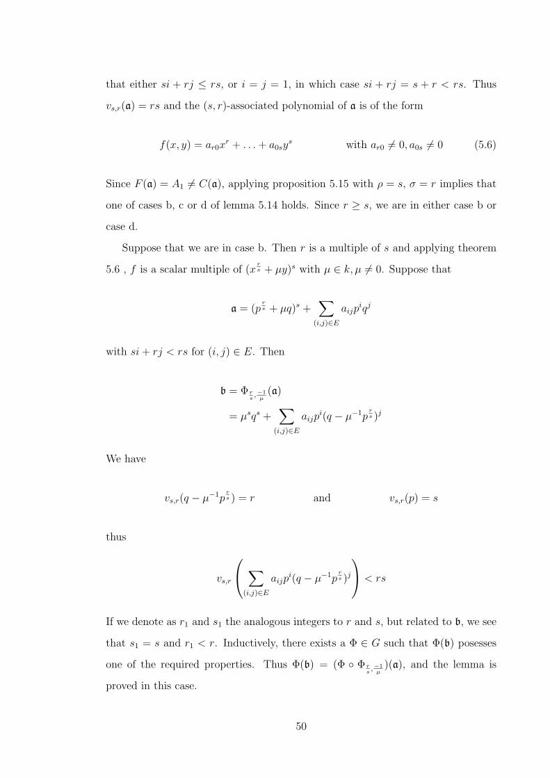
that either si + rj ≤ rs, or i = j = 1, in which case si + rj = s + r < rs. Thus

vs,r(a) = rs and the (s, r)-associated polynomial of a is of the form

f(x, y) = ar0xr + . . .+ a0sy

s with ar0 6= 0, a0s 6= 0 (5.6)

Since F (a) = A1 6= C(a), applying proposition 5.15 with ρ = s, σ = r implies that

one of cases b, c or d of lemma 5.14 holds. Since r ≥ s, we are in either case b or

case d.

Suppose that we are in case b. Then r is a multiple of s and applying theorem

5.6 , f is a scalar multiple of (xrs + µy)s with µ ∈ k, µ 6= 0. Suppose that

a = (prs + µq)s +

∑(i,j)∈E

aijpiqj

with si+ rj < rs for (i, j) ∈ E. Then

b = Φ rs,−1

µ(a)

= µsqs +∑

(i,j)∈E

aijpi(q − µ−1p

rs )j

We have

vs,r(q − µ−1prs ) = r and vs,r(p) = s

thus

vs,r

∑(i,j)∈E

aijpi(q − µ−1p

rs )j

< rs

If we denote as r1 and s1 the analogous integers to r and s, but related to b, we see

that s1 = s and r1 < r. Inductively, there exists a Φ ∈ G such that Φ(b) posesses

one of the required properties. Thus Φ(b) = (Φ ◦ Φ rs,−1

µ)(a), and the lemma is

proved in this case.

50

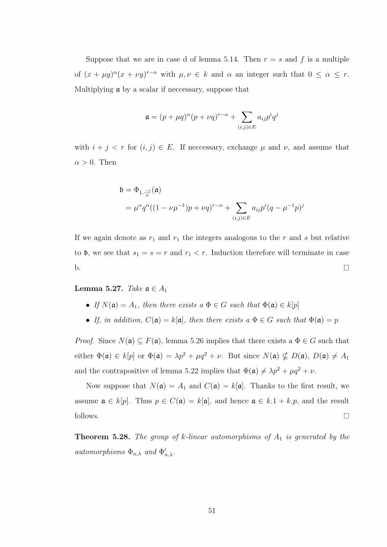
Suppose that we are in case d of lemma 5.14. Then r = s and f is a multiple

of (x + µy)α(x + νy)r−α with µ, ν ∈ k and α an integer such that 0 ≤ α ≤ r.

Multiplying a by a scalar if neccessary, suppose that

a = (p+ µq)α(p+ νq)r−α +∑

(i,j)∈E

aijpiqj

with i + j < r for (i, j) ∈ E. If neccessary, exchange µ and ν, and assume that

α > 0. Then

b = Φ1,−1µ

(a)

= µαqα((1− νµ−1)p+ νq)r−α +∑

(i,j)∈E

aijpi(q − µ−1p)j

If we again denote as r1 and r1 the integers analogous to the r and s but relative

to b, we see that s1 = s = r and r1 < r. Induction therefore will terminate in case

b.

Lemma 5.27. Take a ∈ A1

• If N(a) = A1, then there exists a Φ ∈ G such that Φ(a) ∈ k[p]

• If, in addition, C(a) = k[a], then there exists a Φ ∈ G such that Φ(a) = p

Proof. Since N(a) ⊆ F (a), lemma 5.26 implies that there exists a Φ ∈ G such that

either Φ(a) ∈ k[p] or Φ(a) = λp2 + µq2 + ν. But since N(a) * D(a), D(a) 6= A1

and the contrapositive of lemma 5.22 implies that Φ(a) 6= λp2 + µq2 + ν.

Now suppose that N(a) = A1 and C(a) = k[a]. Thanks to the first result, we

assume a ∈ k[p]. Thus p ∈ C(a) = k[a], and hence a ∈ k.1 + k.p, and the result

follows.

Theorem 5.28. The group of k-linear automorphisms of A1 is generated by the

automorphisms Φn,λ and Φ′n,λ.

51

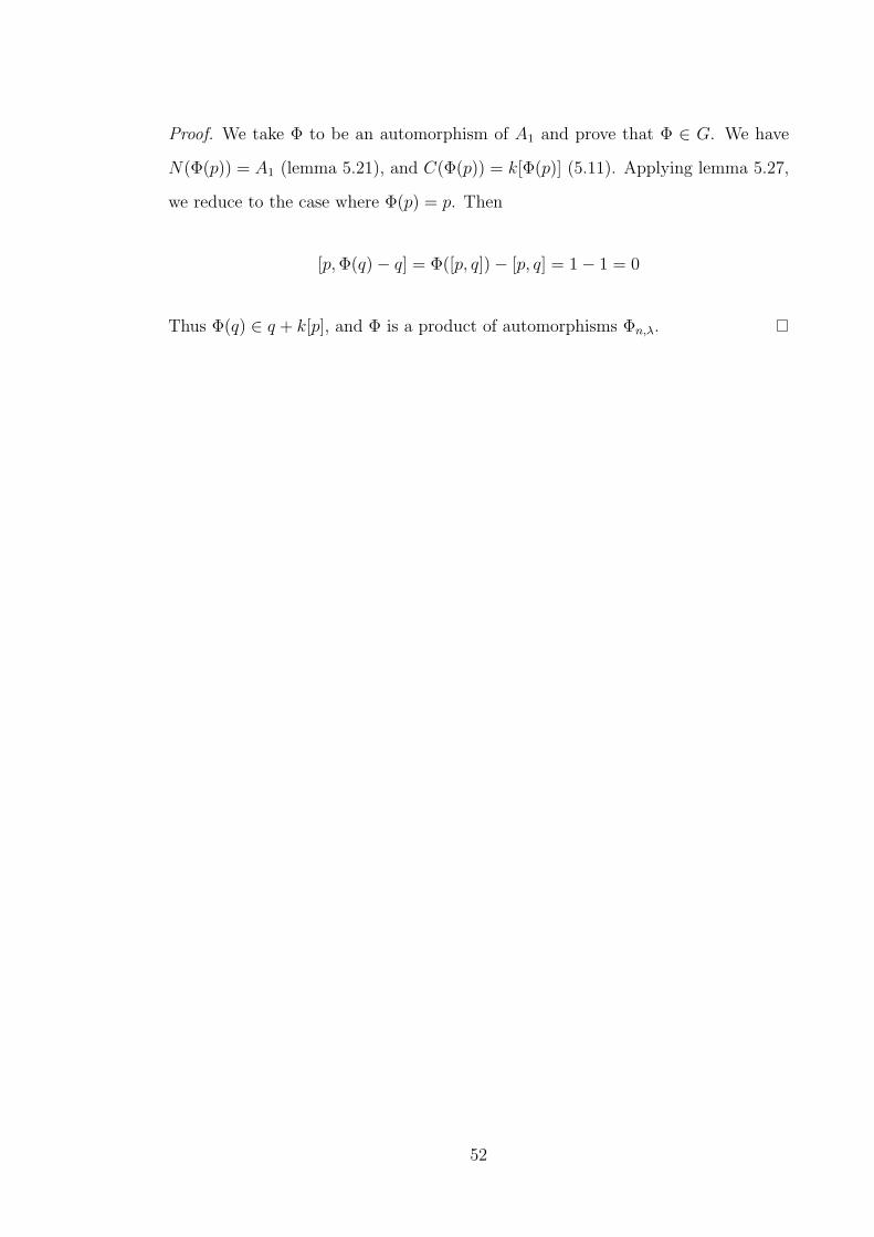
Proof. We take Φ to be an automorphism of A1 and prove that Φ ∈ G. We have

N(Φ(p)) = A1 (lemma 5.21), and C(Φ(p)) = k[Φ(p)] (5.11). Applying lemma 5.27,

we reduce to the case where Φ(p) = p. Then

[p,Φ(q)− q] = Φ([p, q])− [p, q] = 1− 1 = 0

Thus Φ(q) ∈ q + k[p], and Φ is a product of automorphisms Φn,λ.

52

References

[1] Jacques Dixmier, Sur les algebres de Weyl, Bull. Soc. Math. France 96 (1968),

209–247. MR MR0242897 (39 #4224)

[2] Gunter R. Krause and Thomas H. Lenagan, Growth of algebras and Gelfand-

Kirillov dimension, revised ed., Graduate Studies in Mathematics, vol. 22,

American Mathematical Society, Providence, RI, 2000. MR MR1721834

(2000j:16035)

[3] T. Y. Lam, A first course in noncommutative rings, first ed., Graduate texts in

mathematics, vol. 131, Springer-Verlag, New York, 1991.

[4] Dmitriy Rumynin, Rings and modules, (2003).

53