
The visits to zero of a random walk driven by an irrational rotation
46
THE VISITS TO ZERO OF A RANDOM WALK DRIVEN BY AN IRRATIONAL ROTATION A. AVILA, D. DOLGOPYAT, E. DURYEV, AND O. SARIG Abstract. We give a detailed analysis of the returns to zero of the “determin- istic random walk” Sn(x)= ∑ n-1 k=0 f (x + kα) where α is a quadratic irrational, f (x)=1 [ 1 2 ,1) ({x}) - 1 [0, 1 2 ) ({x}), and x is sampled uniformly in [0, 1]. The method is to find the asymptotic behavior of the ergodic sums of L 1 functions for linear flows on the infinite staircase surface. Our methods also provide a new proof of J. Beck’s central limit theorem for Sn(0) where n ∈{1,...,N } is uniform and N →∞, and they allow us to determine the generic points for certain infinite measure preserving skew products (“cylinder maps”). 1. Introduction and overview The simple random walk (SRW) can be generated from a dynamical system as follows. Pick x in T := R/Z uniformly, and iterate the angle doubling map τ : T → T, τ (x)=2x mod 1. Place a “walker” at 0 ∈ Z. At time step k (k ≥ 0), ask the walker to make one step to the left if τ k (x) ∈ [0, 1 2 ), and one step to the right if τ k (x) ∈ [ 1 2 , 1). This procedure generates the simple random walk, because the steps are s k := (-1) x k +1 where 0.x 0 x 1 x 2 ··· is the binary expansion of x, and if x ∈ T is chosen uniformly, then s k are independent random variables, equal to +1 or -1 with probability 1 2 . The angle doubling map is a standard example of a “chaotic” map: It is mixing, it has positive entropy, and it has countable Lebesgue spectrum. It is natural to ask what happens if we replace τ by an “non-chaotic” ergodic map, such as the irrational rotation R α : T → T, R α (x)= x + α mod 1 (α ∈ R \ Q fixed). R α is not mixing, it has zero entropy, and its spectrum is discrete, properties associated with “determinism” (see [Pet] page 245). If we replace τ by R α , then we obtain a stochastic process called the deterministic random walk [AK]. To define it formally, let B denote the Borel σ–algebra of T, let m T be the normalized Lebesgue measure on T thought of as the unit interval mod 1, and define f : T → Z by f (x)= ( -1 x ∈ [0, 1 2 ) +1 x ∈ [ 1 2 , 1). Key words and phrases. uniform distribution,cylinder maps,translation surfaces. A.A. was partially supported by the ERC Starting Grant “Quasiperiodic” and by the Balzan project of Jacob Palis. D.D. was partially supported by the NSF grant DMS 1101635. E.D. was supported by the Kupcinet-Getz summer program at the Weizmann Institute. O.S. was partially supported by ERC Starting Grant “ErgodicNonCompact”. 1
Transcript of The visits to zero of a random walk driven by an irrational rotation
THE VISITS TO ZERO OF A RANDOM WALK DRIVEN BY AN
IRRATIONAL ROTATION
A. AVILA, D. DOLGOPYAT, E. DURYEV, AND O. SARIG
Abstract. We give a detailed analysis of the returns to zero of the “determin-
istic random walk” Sn(x) =∑n−1k=0 f(x+kα) where α is a quadratic irrational,
f(x) = 1[ 12,1)(x)− 1[0, 1
2)(x), and x is sampled uniformly in [0, 1].
The method is to find the asymptotic behavior of the ergodic sums of L1
functions for linear flows on the infinite staircase surface.
Our methods also provide a new proof of J. Beck’s central limit theoremfor Sn(0) where n ∈ 1, . . . , N is uniform and N → ∞, and they allow us
to determine the generic points for certain infinite measure preserving skewproducts (“cylinder maps”).
1. Introduction and overview
The simple random walk (SRW) can be generated from a dynamical system asfollows. Pick x in T := R/Z uniformly, and iterate the angle doubling map
τ : T→ T, τ(x) = 2x mod 1.
Place a “walker” at 0 ∈ Z. At time step k (k ≥ 0), ask the walker to make onestep to the left if τk(x) ∈ [0, 1
2 ), and one step to the right if τk(x) ∈ [ 12 , 1). This
procedure generates the simple random walk, because the steps are sk := (−1)xk+1
where 0.x0x1x2 · · · is the binary expansion of x, and if x ∈ T is chosen uniformly,then sk are independent random variables, equal to +1 or −1 with probability 1
2 .The angle doubling map is a standard example of a “chaotic” map: It is mixing,
it has positive entropy, and it has countable Lebesgue spectrum. It is natural toask what happens if we replace τ by an “non-chaotic” ergodic map, such as theirrational rotation
Rα : T→ T, Rα(x) = x+ α mod 1 (α ∈ R \Q fixed).
Rα is not mixing, it has zero entropy, and its spectrum is discrete, propertiesassociated with “determinism” (see [Pet] page 245).
If we replace τ by Rα, then we obtain a stochastic process called the deterministicrandom walk [AK]. To define it formally, let B denote the Borel σ–algebra of T,let mT be the normalized Lebesgue measure on T thought of as the unit intervalmod 1, and define f : T→ Z by
f(x) =
−1 x ∈ [0, 1
2 )
+1 x ∈ [ 12 , 1).
Key words and phrases. uniform distribution,cylinder maps,translation surfaces.A.A. was partially supported by the ERC Starting Grant “Quasiperiodic” and by the Balzan
project of Jacob Palis. D.D. was partially supported by the NSF grant DMS 1101635. E.D. was
supported by the Kupcinet-Getz summer program at the Weizmann Institute. O.S. was partiallysupported by ERC Starting Grant “ErgodicNonCompact”.
1
2 A. AVILA, D. DOLGOPYAT, E. DURYEV, AND O. SARIG
The deterministic random walk (DRW) with angle α ∈ R \ Q is the sequence
S0 = 0, Sn =∑n−1k=0 f Rkα (n ≥ 1) on the probability space (T,B,mT). The
following table compares it with the simple random walk:
Simple RW Deterministic RWA.e. orbit returns to zero. A.e. orbit returns to zero [At].
Recurrence The set of exceptions has full The set of exceptions isHausdorff dimension [BS] finite [Ra].
Trace Z for a.e. x, Z for a.e. x [C],[CK],[Sch],Sn(x) : n ≥ 0 but not for all x. but not for all x [BR],[Pe].Drift A.e. orbit has zero drift. All orbits have zero driftlimn→∞
Sn(x)/n The set of exceptions has full by Weyl’s Theorem
Hausdorff dimension [BS] ([KN, chapter 1])Central No, by the Denjoy–KoksmaLimit Yes Ineq. [Her, page 73]. OtherTheorem choices of f may have CLT
[BD],[V]. See also [Hu],[B1]
In this paper we contribute to the study of the visits to zero of the deterministicrandom walk: Nn(x) = Nn(x;α) := #0 ≤ k ≤ n− 1 : Sk(x) = 0.
For the simple random walk, if the number of visits to zero up to time n is
Nn, then E(Nn) ∼√
2n/π (de Moivre–Laplace Theorem), and 1√nNn
dist−−−−→n→∞
Θ(1),
where Θ(t) is Brownian local time [Bor]. The deterministic random walk behavesdifferently. Aaronson and Keane showed in [AK] that if α is a quadratic irrational,then there are constants c1, c2 > 0 s.t. c1( n√
lnn) ≤ E(Nn) ≤ c2( n√
lnn).
We show, among other things, that if α is a quadratic irrational, then there is apositive constant c(α) with the following properties:
(1) E(Nn) ∼ c(α)( n√lnn
) =: an(α) as n→∞.
(2) 1an(α)Nn
dist−−−−→n→∞
√2 exp[− 1
2χ2], where χ has the standard normal distribution.
(3) 1ln lnm
∑m−1n=0
1n lnn
(1
an(α)Nn
)−−−−→m→∞
1 almost surely.
(4) c(α) =√| lnλ|4πσ2 where λ, σ2 ∈ Q[α] can be calculated explicitly. For example,
c(√
2) =
√√2
3π ln(17 + 12√
2).
These results should be contrasted with Kesten’s work [Kes] which says that ifα is also randomized (i.e. (x, α) chosen uniformly in [0, 1]2), then the right scalingfor Nn(x;α) is n/ lnn.
Our main tool is the cylinder map Tα(x, ξ) = (x+α mod 1, ξ+ f(x)) on T×Z,together with the (infinite) invariant measure mT×Z := mT ×mZ (mT=normalizedLebesgue measure on T, mZ =counting measure on Z). To see the connection tothe DRW, write Tnα := Tα · · · Tα (n times) and observe by direct calculation that
• Sn(x) is the second coordinate of Tnα (x, 0), and
• Nn(x) =∑n−1k=0 1T×0(T
kα(x, 0)), where 1E is the indicator function of E.
We will analyze the asymptotic behavior of SnG :=∑n−1k=0 G T kα for general non-
negative functions G ∈ L1(T× Z). The results for Nn follow from the special caseG = 1T×0.
A RANDOM WALK DRIVEN BY AN IRRATIONAL ROTATION 3
(c)“up”
(a)
1 1
i
i
4 4
iv
iv
2 2
ii
ii
5 5
v
vi
v
3 3
iii
iii
(b) 1
1
1
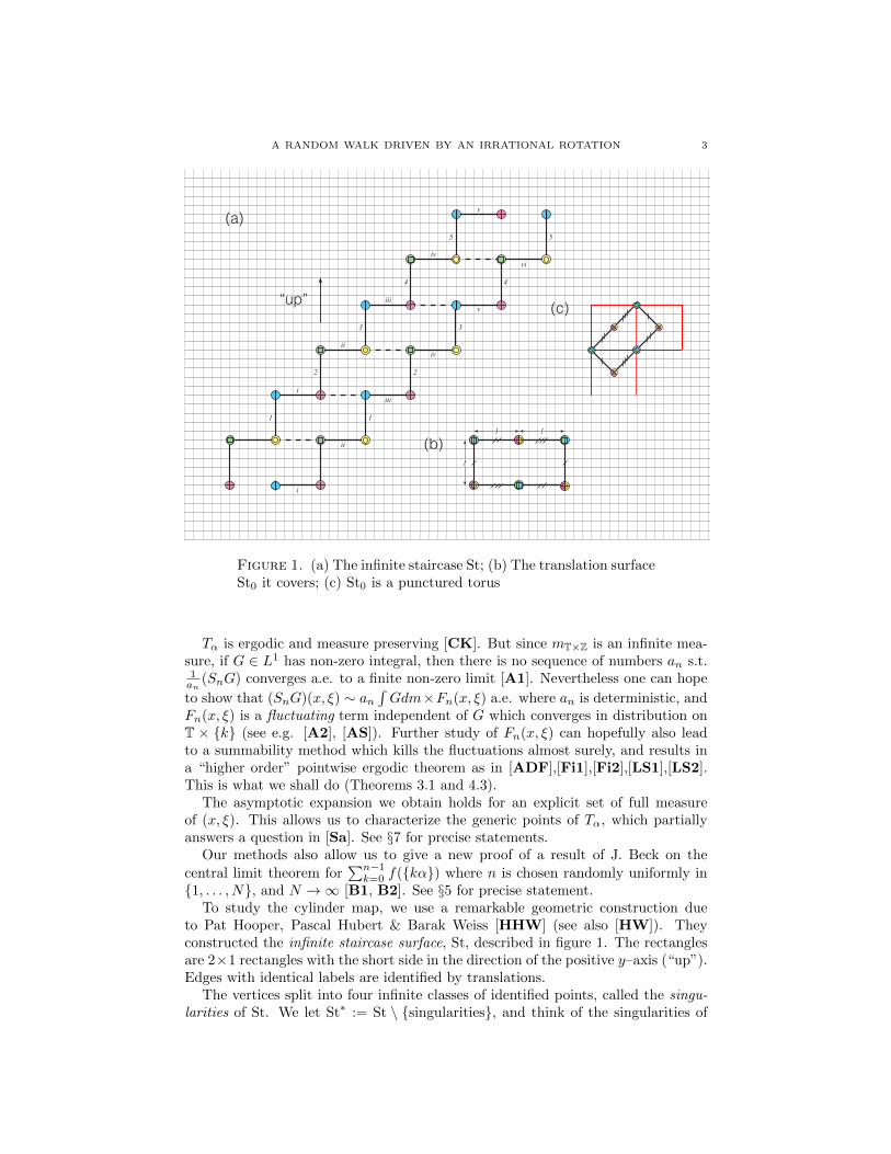
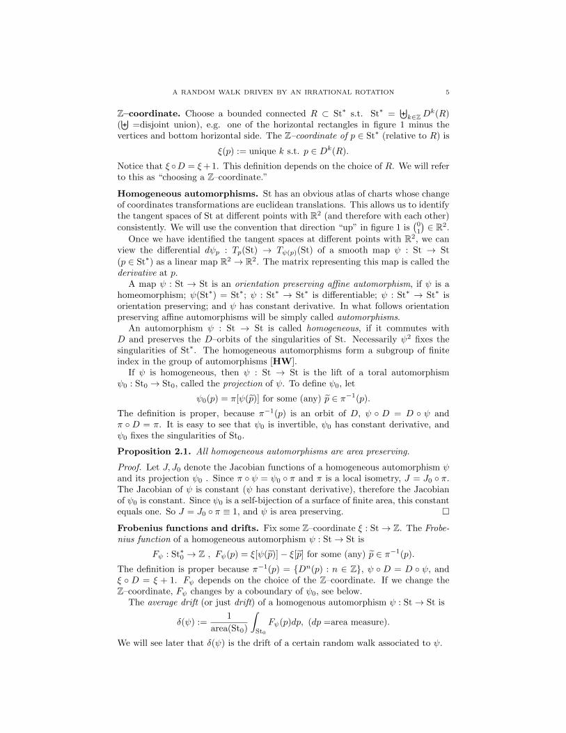
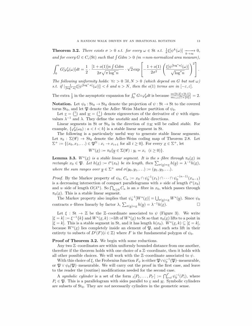
Figure 1. (a) The infinite staircase St; (b) The translation surfaceSt0 it covers; (c) St0 is a punctured torus
Tα is ergodic and measure preserving [CK]. But since mT×Z is an infinite mea-sure, if G ∈ L1 has non-zero integral, then there is no sequence of numbers an s.t.1an
(SnG) converges a.e. to a finite non-zero limit [A1]. Nevertheless one can hope
to show that (SnG)(x, ξ) ∼ an∫Gdm×Fn(x, ξ) a.e. where an is deterministic, and
Fn(x, ξ) is a fluctuating term independent of G which converges in distribution onT × k (see e.g. [A2], [AS]). Further study of Fn(x, ξ) can hopefully also leadto a summability method which kills the fluctuations almost surely, and results ina “higher order” pointwise ergodic theorem as in [ADF],[Fi1],[Fi2],[LS1],[LS2].This is what we shall do (Theorems 3.1 and 4.3).
The asymptotic expansion we obtain holds for an explicit set of full measureof (x, ξ). This allows us to characterize the generic points of Tα, which partiallyanswers a question in [Sa]. See §7 for precise statements.
Our methods also allow us to give a new proof of a result of J. Beck on thecentral limit theorem for
∑n−1k=0 f(kα) where n is chosen randomly uniformly in
1, . . . , N, and N →∞ [B1, B2]. See §5 for precise statement.To study the cylinder map, we use a remarkable geometric construction due
to Pat Hooper, Pascal Hubert & Barak Weiss [HHW] (see also [HW]). Theyconstructed the infinite staircase surface, St, described in figure 1. The rectanglesare 2×1 rectangles with the short side in the direction of the positive y–axis (“up”).Edges with identical labels are identified by translations.
The vertices split into four infinite classes of identified points, called the singu-larities of St. We let St∗ := St \ singularities, and think of the singularities of
4 A. AVILA, D. DOLGOPYAT, E. DURYEV, AND O. SARIG
St as of punctures in St∗. Each singularity is the meeting point of infinitely manyrectangles, and the angle around it is infinite.
The linear flow at direction θ ∈ (−π2 ,π2 ) is the flow ϕtθ which moves a point on
St∗ in the direction(
sin θcos θ
)t units of distance respecting identifications (θ = 0 is
moving “up”). The definition makes sense for the set of full measure of points pwhose orbit does not hit a singularity.
The connection to the cylinder map is explained by the following observationfrom [HHW]. Recall that a Poincare section for ϕθ is a set S ⊂ St s.t. for a.e. p ∈St there is a minimal positive time r(p) > 0 s.t. ϕ
r(p)θ (p) ∈ S, and infp∈S r(p) > 0.
The function r : S → (0,∞) and the map T : S → S, T (p) = ϕr(p)θ (p), are called
the roof function and Poincare map of S.
Lemma 1.1. For θ 6= ±π2 +2πk, the union of the horizontal sides of the horizontalrectangles in figure 1 is a Poincare section for ϕθ with constant roof function. ThePoincare map is isomorphic to the cylinder map Tα where α = 1
2 tan θ + 12 .
The isomorphism is very simple: Divide St into horizontal rectangles, call one ofthem “rectangle zero” and tag the remaining rectangles by ξ ∈ Z in such a way thatthe rectangle directly above rectangle ξ is rectangle ξ+ 1. The point (x, ξ) ∈ T×Zcorresponds to the point ω(x) on the top horizontal side of rectangle ξ, and located2x units of distance away from the left end.
Since Tα is a Poincare map for ϕθ with constant roof function, there is a standardway to reduce the study of the Birkhoff sums of Tα to the analysis of the Birkhoffintegrals of ϕθ. This is what we will do.
The gain in the reduction to the infinite staircase model is that St has manysymmetries which are hidden for the DRW: For special directions θ, it is possibleto find a “nice” automorphism ψ : St→ St s.t. for some 0 < λ < 1
ψ ϕtθ = ϕλtθ ψ. (∗)
This is what happens for the θ whose corresponding α is a quadratic irrational.(∗) is the key to the asymptotic behavior of the Birkhoff sums of ϕθ and Tα, andtherefore also to the asymptotic behavior of the visits to zero of the DRW.
2. The infinite staircase and its automorphisms
Z–cover. St∗ is a regular Z–cover of a finite area surface St∗0 (figure 1(b)). Let
π : St∗ → St∗0
be the covering map. St∗0 is a twice punctured torus (Figure 1(c)). Let St0 denotethe completion of St∗0 with respect to the natural metric. St0 is a torus, andπ : St∗ → St∗0 extends continuously to a map π : St → St0. The extension istwo-to-one on the singularities of St and infinite-to-one elsewhere.
The group of deck transformations of the covering is generated by an obvioustranslation. We denote it by
D : St→ St.
D2 fixes the singularities.
A RANDOM WALK DRIVEN BY AN IRRATIONAL ROTATION 5
Z–coordinate. Choose a bounded connected R ⊂ St∗ s.t. St∗ =⊎k∈ZD
k(R)(⊎
=disjoint union), e.g. one of the horizontal rectangles in figure 1 minus thevertices and bottom horizontal side. The Z–coordinate of p ∈ St∗ (relative to R) is
ξ(p) := unique k s.t. p ∈ Dk(R).
Notice that ξ D = ξ+ 1. This definition depends on the choice of R. We will referto this as “choosing a Z–coordinate.”
Homogeneous automorphisms. St has an obvious atlas of charts whose changeof coordinates transformations are euclidean translations. This allows us to identifythe tangent spaces of St at different points with R2 (and therefore with each other)consistently. We will use the convention that direction “up” in figure 1 is
(01
)∈ R2.
Once we have identified the tangent spaces at different points with R2, we canview the differential dψp : Tp(St) → Tψ(p)(St) of a smooth map ψ : St → St
(p ∈ St∗) as a linear map R2 → R2. The matrix representing this map is called thederivative at p.
A map ψ : St → St is an orientation preserving affine automorphism, if ψ is ahomeomorphism; ψ(St∗) = St∗; ψ : St∗ → St∗ is differentiable; ψ : St∗ → St∗ isorientation preserving; and ψ has constant derivative. In what follows orientationpreserving affine automorphisms will be simply called automorphisms.
An automorphism ψ : St → St is called homogeneous, if it commutes withD and preserves the D–orbits of the singularities of St. Necessarily ψ2 fixes thesingularities of St∗. The homogeneous automorphisms form a subgroup of finiteindex in the group of automorphisms [HW].
If ψ is homogeneous, then ψ : St → St is the lift of a toral automorphismψ0 : St0 → St0, called the projection of ψ. To define ψ0, let
ψ0(p) = π[ψ(p)] for some (any) p ∈ π−1(p).
The definition is proper, because π−1(p) is an orbit of D, ψ D = D ψ andπ D = π. It is easy to see that ψ0 is invertible, ψ0 has constant derivative, andψ0 fixes the singularities of St0.
Proposition 2.1. All homogeneous automorphisms are area preserving.
Proof. Let J, J0 denote the Jacobian functions of a homogeneous automorphism ψand its projection ψ0 . Since π ψ = ψ0 π and π is a local isometry, J = J0 π.The Jacobian of ψ is constant (ψ has constant derivative), therefore the Jacobianof ψ0 is constant. Since ψ0 is a self-bijection of a surface of finite area, this constantequals one. So J = J0 π ≡ 1, and ψ is area preserving.
Frobenius functions and drifts. Fix some Z–coordinate ξ : St→ Z. The Frobe-nius function of a homogeneous automorphism ψ : St→ St is
Fψ : St∗0 → Z , Fψ(p) = ξ[ψ(p)]− ξ[p] for some (any) p ∈ π−1(p).
The definition is proper because π−1(p) = Dn(p) : n ∈ Z, ψ D = D ψ, andξ D = ξ + 1. Fψ depends on the choice of the Z–coordinate. If we change theZ–coordinate, Fψ changes by a coboundary of ψ0, see below.
The average drift (or just drift) of a homogenous automorphism ψ : St→ St is
δ(ψ) :=1
area(St0)
∫St0
Fψ(p)dp, (dp =area measure).
We will see later that δ(ψ) is the drift of a certain random walk associated to ψ.
6 A. AVILA, D. DOLGOPYAT, E. DURYEV, AND O. SARIG
Lemma 2.2. The average drift is independent of the choice of the Z–coordinate,and δ(ψ φ) = δ(ψ) + δ(φ) for any homogeneous automorphisms ψ, φ.
Proof. Let ψ0 : St0 → St0 be the projection of ψ, and suppose ξ, η are two choices
of Z–coordinates with Frobenius functions F ξψ, Fηψ . We claim that
∫F ξψ =
∫F ηψ .
Define ∆ : St0 → Z , ∆(p) = ξ(p) − η(p) for some (any) p ∈ π−1(p). Thedefinition is proper since π−1(p) is aD–orbit, and (ξ−η)D = (ξ+1)−(η+1) = ξ−η.
A simple calculation shows that F ξψ − F ηψ = ∆ ψ0 − ∆. Since ψ0 is measure
preserving,∫
(F ξψ − Fηψ) =
∫(∆ ψ0 −∆) = 0, and
∫F ξψ =
∫F ηψ .
Next suppose ψ, φ are two homogeneous automorphisms. It is easy to see thatψ φ is a homogeneous automorphism, and for every p ∈ St0 and p ∈ π−1(p),
Fψφ(p) = ξ[ψ(φ(p))]− ξ[p] = ξ[ψ(φ(p))]− ξ[φ(p)] + ξ[φ(p)]− ξ[p]= (Fψ φ0)(p) + Fφ(p), where φ0 is the projection of φ.
Since φ0 is area preserving, δ(ψ φ) =∫Fψ φ0 +
∫Fφ = δ(ψ) + δ(φ).
By [HHW] the set of derivatives of homogeneous automorphisms equals
Γ = A ∈ SL(2,Z) : A =(
1 00 1
)or(
0 1−1 0
)mod 2
Here is a refinement of this statement. The proof is in the appendix.
Proposition 2.3 (Classification of homogeneous automorphisms).
(1) If A ∈ SL(2,Z), A =(
1 00 1
)mod 2 and δ0 ∈ Z, then there is a unique homo-
geneous automorphism with derivative A and drift δ0.(2) If A ∈ SL(2,Z), A =
(0 1
−1 0
)mod 2 and δ0 ∈ 1
2 + Z, then there is a uniquehomogeneous automorphism with derivative A and drift δ0.
(3) No other homogeneous automorphisms exist.
Renormalizing hyperbolic automorphisms. A homogeneous automorphism ofSt is called hyperbolic if its derivative matrix has two real eigenvalues, λ, λ−1, where0 < |λ| < 1.
Definition 2.4. A hyperbolic homogeneous automorphism ψ renormalizes α ∈ R,if α = 1
2 + 12 tan θ(mod 1) where
(sin θcos θ
)is an eigenvector of the derivative of ψ. In
this case we say that α is renormalized by ψ.
The motivation is that if α = 12 + 1
2 tan θ(mod 1), then Tα is the Poincare map ofthe linear flow in direction θ, ϕθ : St→ St, and
ψ ϕtθ = ϕλtθ ψwhere λ is the eigenvalue of
(sin θcos θ
).
There is no loss of generality in assuming that (a) the eigenvalues are positive,(b) ψ fixes the singularities of St, (c) ψ has zero drift, and (d) 0 < λ < 1: We sawabove that any homogeneous automorphism ψ has drift in 1
2Z, so 2δ(ψ) is always an
integer. One of the automorphisms D−4δ(ψ)ψ4, D4δ(ψ)ψ−4 satisfies (a),(b),(c),(d).
We characterize the irrational numbers α which possess renormalizing automor-phisms. Recall that a quadratic irrational is an irrational α s.t. aα2 + bα + c = 0for some a, b, c ∈ Z not all equal to zero.
Proposition 2.5. α is renormalized by a hyperbolic homogeneous automorphismiff it is a quadratic irrational.
A RANDOM WALK DRIVEN BY AN IRRATIONAL ROTATION 7
Proof. The derivative of a hyperbolic homogeneous automorphism belongs to SL(2,Z).The eigenvalues of such matrices are quadratic irrationals, and the slopes of theeigenvectors of such matrices are quadratic irrationals. It follows that all irrationalswith renormalizing hyperbolic automorphisms are quadratic.
For the converse suppose that α is a quadratic irrational. We prove that arenormalizing automorphism exists. Let α′ := 1/(2α− 1). This is also a quadraticirrational.
By Lagrange’s Theorem, the continued fraction expansion of α′ is eventually
periodic. So there is a map ϕ(z) = a′z+b′
c′z+d′ with(a′ b′
c′ d′)∈ SL(2,Z) s.t. the
continued fraction expansion of ϕ(α′) is (completely) periodic:
ϕ(α′) = [a0, . . . , an−1, a0, . . . , an−1, · · · ]. (2.1)
Let pkqk
denote the principal convergents of β := ϕ(α′). By the theory of continued
fractions, det(pn pn−1qn qn−1
)= (−1)n+1, and β is a fixed point of ψ(z) = pnz+pn−1
qnz+qn−1.
So ψ[ϕ(α′)] = ϕ(α′), whence (ϕ−1ψϕ)(α′) = α′.Let φ := ϕ−1ψϕ, then φN (α′) = α′ for all N . We claim that for some N , φN is
a Mobius transformation with matrix belonging to
Γ(2) := A ∈ SL(2,Z) : A = Id mod 2.Let A be the matrix which represents φ2. Obviously, φ2 ∈ SL(2,Z). Let [A]2 ∈SL(2,Z2) denote the residue class of A mod 2. The group SL(2,Z2) is finite,therefore [AN ]2 = ([A]2)N = Id for some N . So φ2N is represented by a matrix inΓ(2), proving the claim.
Write φ2N (z) = c+dza+bz for
(d cb a
)∈ Γ(2), then(
a bc d
)(1
α′
)=
(a+ bα′
c+ dα′
)= (a+ bα′)
(1
φ2N (α′)
)= (a+ bα′)
(1
α′
), (2.2)
proving that(
1α′
)is an eigenvector of
(a bc d
)∈ Γ(2). This matrix is hyperbolic,
because its trace is bigger than two: a + d = tr[φ2N
]= tr
[(pn pn−1qn qn−1
)2N],
and every 2× 2 matrix with determinant one and all of whose entries are positiveintegers, has trace bigger than two.
By (2.2), the homogeneous automorphism with zero drift and derivative(a bc d
)renormalizes α = 1
2 + 12 ( 1α′ ).
The previous proof is constructive, but it does not provide a convenient tool forcalculating renormalizing automorphisms. This is the purpose of the next result.
Proposition 2.6. Any quadratic irrational α equals 12 +
k+√q(q+1)
2n (mod 1) for
some k, q, n ∈ Z satisfying q(q + 1) 6= 0 and n|k2 − q(q + 1). In this case there is arenormalizing homogeneous automorphism ψ with zero drift and derivative
dψ =
(2(q − k) + 1 2 · k
2−q(q+1)n
−2n 2(q + k) + 1
). (2.3)
Example: For α =√
2, we can take k = n = 3, q = 8, and get the homogeneousautomorphism with zero drift and derivative
(11 −42−6 23
).
Similar formulas can be obtained for√
3 (k = n = 1, q = 3),√
5 (k = n = 1, q =
4),√
7 (k = n = 12, q = 63) etc.
8 A. AVILA, D. DOLGOPYAT, E. DURYEV, AND O. SARIG
Proof. Since α is a quadratic irrational, it has a hyperbolic renormalizing automor-phism with zero drift. Let A be the derivative. By proposition 2.3, A =
(a bc d
)with a, d odd and b, c even, and ad− bc = 1.
We claim that tr(A) = 2 (mod 4). Since a, d are odd, they are equal to±1 (mod 4).Write a = 4α+ε, d = 4β+η, b = 2γ, c = 2δ with α, β, γ, δ ∈ Z and ε, η = ±1. Since1 = det(A) = εη(mod 4), ε = η. It follows that a = d(mod 4) and trA = a + d =4(α+ β)± 2 ∈ 4Z + 2.
Write tr(A) = 4q + 2 with some q ∈ Z. Since a, d are odd and a + d = 4q + 2,we can put a, d in the form a = 2(q − k) + 1 and d = 2(q + k) + 1 with k ∈ Z.
Since c is even, c = −2n with some n ∈ Z. Since ad− bc = 1, either n = 0 and
A = Id, or n 6= 0 and b = 2 · k2−q(q+1)
n . So A =
(2(q − k) + 1 2 · k
2−q(q+1)n
−2n 2(q + k) + 1
)with q, n, k ∈ Z s.t. n 6= 0 and n|k2 − q(q + 1). Such choice of k, q, n determines a
matrix in SL(2,Z) equal to(
1 00 1
)mod 2.
The characteristic polynomial of A is x2 − x trA + detA = x2 − (4q + 2)x +
1. The eigenvalues are (2q + 1) ± 2√q(q + 1). A is hyperbolic iff q(q + 1) 6= 0.
The eigenvectors are proportional to (k±√q(q+1)
n , 1), so the automorphism with
derivative A renormalizes α := 12 +
k±√q(q+1)
n . Playing with the signs of k, n we
see that there is no loss in taking α := 12 +
k+√q(q+1)
n .
Markov partitions and symbolic dynamics. Every hyperbolic homogeneousautomorphism ψ : St→ St covers a hyperbolic toral automorphism ψ0 : St0 → St0.Adler and Weiss introduced in [AW] a technique for coding ψ0 : St0 → St0 as theaction of the left shift map on the collection of two sided infinite paths on a finitedirected graph. This is done using Markov partitions. The purpose of this sectionis to describe this method.
The original work of Adler & Weiss applies to general hyperbolic automorphisms.It is important for our purposes to apply the Adler–Weiss construction in a waywhich respects that fact that ψ0 fixes the punctures of St0 and has derivative matrix
A ∈ Γ(2) := A ∈ SL(2,Z) : A =(
1 00 1
)mod 2.
We will assume for simplicity that A has positive eigenvalues, 0 < λ < 1 andλ−1 > 1. Then there are vectors v =
(1v
), w =
(1w
)such that Av = λ−1v and
Aw = λw. Since A ∈ Γ(2), v, w are irrational. We call w the stable direction and vthe unstable direction (of ψ0).
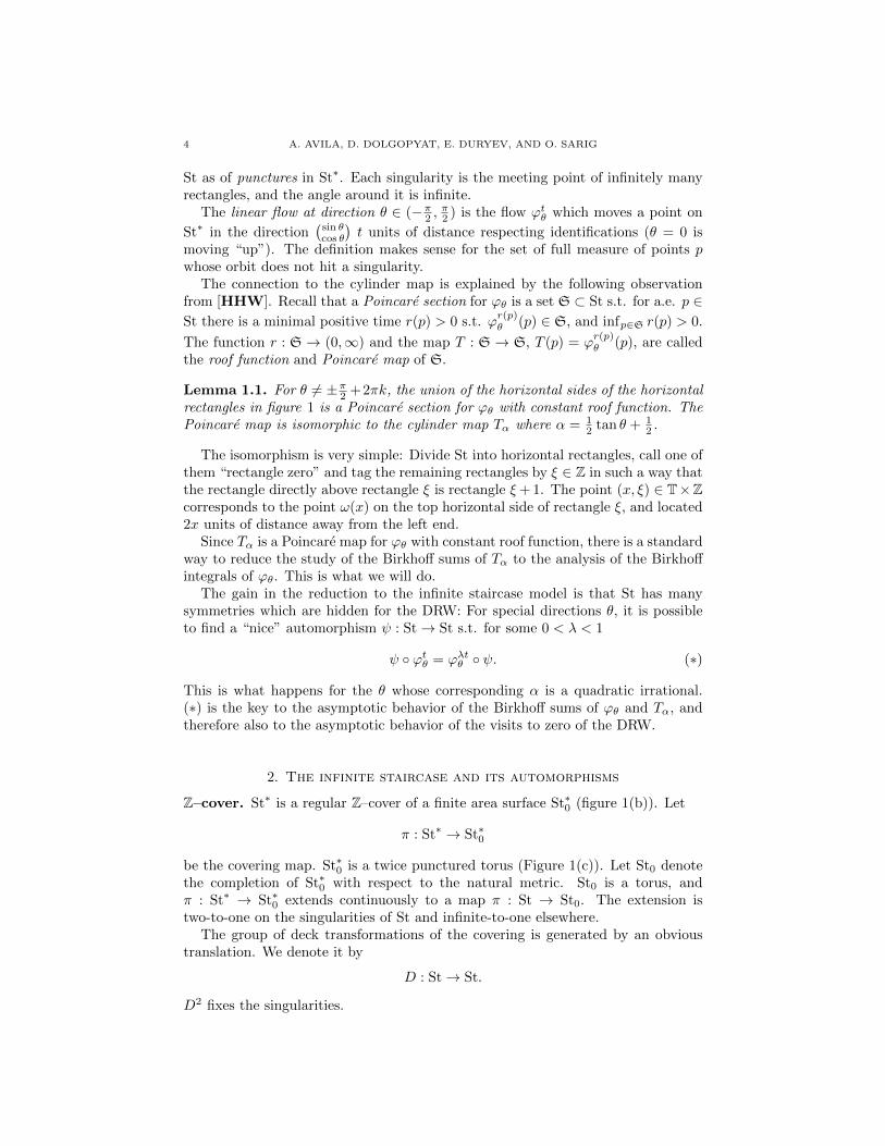
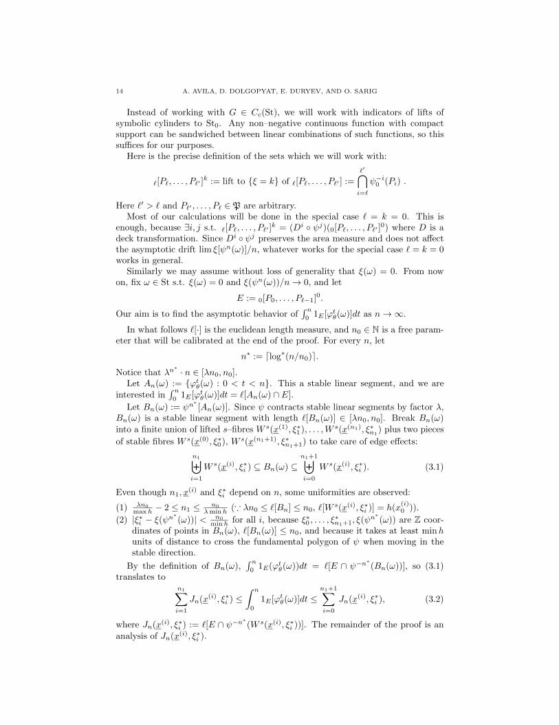
The first step in the Adler–Weiss construction is to divide the torus into twoparallelograms Q1, Q2 with sides parallel to v, w. They cut the torus along two linesegments emanating from a single fixed point. We prefer to use one segment passingthrough the first puncture, and the other passing through the second puncture: thissimplifies the analysis of the coded Frobenius function, see §6 below.
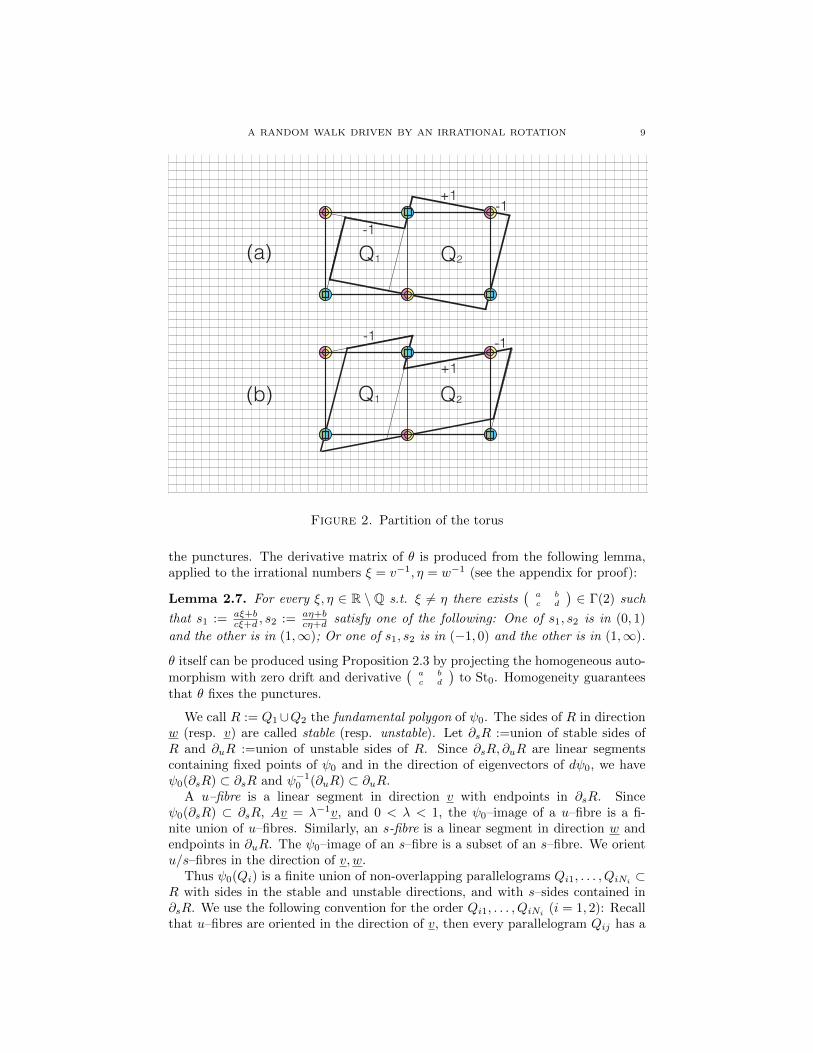
Suppose first that −1 < w < 0, v > 1 (case 1), or 0 < w < 1, v > 1 (case 2).Then Q1, Q2 can be constructed as in Figure 2. One of the parallelograms, whichwe call Q1, does not contain any punctures in its top or bottom sides. The other,which we call Q2, does.
The general case can be reduced to case 1 or 2 by working with θ ψ0 θ−1
or θ ψ−10 θ−1 for a suitable toral automorphism θ : St0 → St0 which fixes
A RANDOM WALK DRIVEN BY AN IRRATIONAL ROTATION 9
(a)
(b) Q1 Q2
-1
+1
-1
Q1 Q2
-1
+1-1
Figure 2. Partition of the torus
the punctures. The derivative matrix of θ is produced from the following lemma,applied to the irrational numbers ξ = v−1, η = w−1 (see the appendix for proof):
Lemma 2.7. For every ξ, η ∈ R \ Q s.t. ξ 6= η there exists(a bc d
)∈ Γ(2) such
that s1 := aξ+bcξ+d , s2 := aη+b
cη+d satisfy one of the following: One of s1, s2 is in (0, 1)
and the other is in (1,∞); Or one of s1, s2 is in (−1, 0) and the other is in (1,∞).
θ itself can be produced using Proposition 2.3 by projecting the homogeneous auto-morphism with zero drift and derivative
(a bc d
)to St0. Homogeneity guarantees
that θ fixes the punctures.
We call R := Q1∪Q2 the fundamental polygon of ψ0. The sides of R in directionw (resp. v) are called stable (resp. unstable). Let ∂sR :=union of stable sides ofR and ∂uR :=union of unstable sides of R. Since ∂sR, ∂uR are linear segmentscontaining fixed points of ψ0 and in the direction of eigenvectors of dψ0, we haveψ0(∂sR) ⊂ ∂sR and ψ−1
0 (∂uR) ⊂ ∂uR.A u–fibre is a linear segment in direction v with endpoints in ∂sR. Since
ψ0(∂sR) ⊂ ∂sR, Av = λ−1v, and 0 < λ < 1, the ψ0–image of a u–fibre is a fi-nite union of u–fibres. Similarly, an s-fibre is a linear segment in direction w andendpoints in ∂uR. The ψ0–image of an s–fibre is a subset of an s–fibre. We orientu/s–fibres in the direction of v, w.
Thus ψ0(Qi) is a finite union of non-overlapping parallelograms Qi1, . . . , QiNi ⊂R with sides in the stable and unstable directions, and with s–sides contained in∂sR. We use the following convention for the order Qi1, . . . , QiNi (i = 1, 2): Recallthat u–fibres are oriented in the direction of v, then every parallelogram Qij has a
10 A. AVILA, D. DOLGOPYAT, E. DURYEV, AND O. SARIG
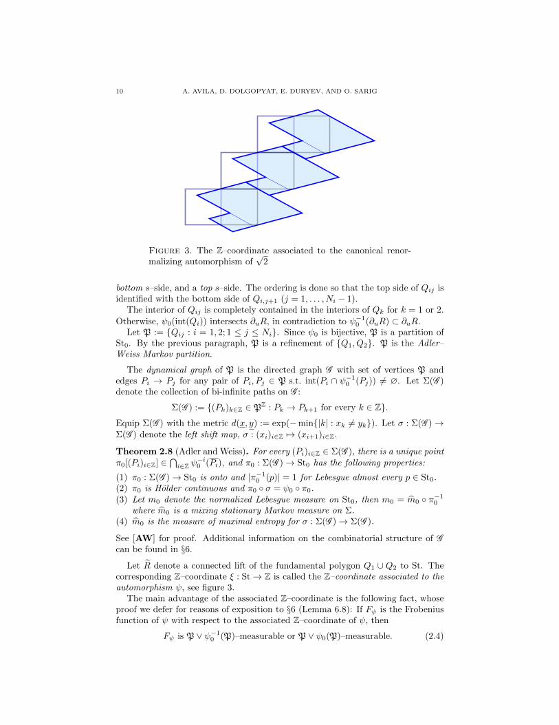
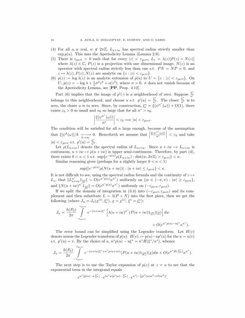
Figure 3. The Z–coordinate associated to the canonical renor-malizing automorphism of
√2
bottom s–side, and a top s–side. The ordering is done so that the top side of Qij isidentified with the bottom side of Qi,j+1 (j = 1, . . . , Ni − 1).
The interior of Qij is completely contained in the interiors of Qk for k = 1 or 2.
Otherwise, ψ0(int(Qi)) intersects ∂uR, in contradiction to ψ−10 (∂uR) ⊂ ∂uR.
Let P := Qij : i = 1, 2; 1 ≤ j ≤ Ni. Since ψ0 is bijective, P is a partition ofSt0. By the previous paragraph, P is a refinement of Q1, Q2. P is the Adler–Weiss Markov partition.
The dynamical graph of P is the directed graph G with set of vertices P andedges Pi → Pj for any pair of Pi, Pj ∈ P s.t. int(Pi ∩ ψ−1
0 (Pj)) 6= ∅. Let Σ(G )denote the collection of bi-infinite paths on G :
Σ(G ) := (Pk)k∈Z ∈ PZ : Pk → Pk+1 for every k ∈ Z.
Equip Σ(G ) with the metric d(x, y) := exp(−min|k| : xk 6= yk). Let σ : Σ(G )→Σ(G ) denote the left shift map, σ : (xi)i∈Z 7→ (xi+1)i∈Z.
Theorem 2.8 (Adler and Weiss). For every (Pi)i∈Z ∈ Σ(G ), there is a unique pointπ0[(Pi)i∈Z] ∈
⋂i∈Z ψ
−i0 (Pi), and π0 : Σ(G )→ St0 has the following properties:
(1) π0 : Σ(G )→ St0 is onto and |π−10 (p)| = 1 for Lebesgue almost every p ∈ St0.
(2) π0 is Holder continuous and π0 σ = ψ0 π0.(3) Let m0 denote the normalized Lebesgue measure on St0, then m0 = m0 π−1
0
where m0 is a mixing stationary Markov measure on Σ.(4) m0 is the measure of maximal entropy for σ : Σ(G )→ Σ(G ).
See [AW] for proof. Additional information on the combinatorial structure of Gcan be found in §6.
Let R denote a connected lift of the fundamental polygon Q1 ∪ Q2 to St. Thecorresponding Z–coordinate ξ : St→ Z is called the Z–coordinate associated to theautomorphism ψ, see figure 3.
The main advantage of the associated Z–coordinate is the following fact, whoseproof we defer for reasons of exposition to §6 (Lemma 6.8): If Fψ is the Frobeniusfunction of ψ with respect to the associated Z–coordinate of ψ, then
Fψ is P ∨ ψ−10 (P)–measurable or P ∨ ψ0(P)–measurable. (2.4)
A RANDOM WALK DRIVEN BY AN IRRATIONAL ROTATION 11
This means there exists a function g : P×P→ Z s.t. the coded Frobenius function
F := Fψ π0 : Σ(G )→ Z
takes the form F [P ] = g(P0, P1) or F [P ] = g(P−1, P0), where P = (Pi)i∈Z ∈ Σ(G ).
The following additional property of F is proved in the appendix.
Lemma 2.9 (Aperiodicity Lemma). If eitF = zh/h σ where |z| = 1, t ∈ R, andh : Σ(G )→ C is continuous , then z = 1, t ∈ 2πZ, and h = const.
This is called the aperiodicity condition in [GH], and should be viewed as a strongway of saying that F does not take values in a set of the form a + bZ “up to acoboundary.” The aperiodicity condition is used in §3, to show that σ 6= 0.
The twist at a singularity. The contents of this section are only used in §5.Suppose ψ is a homogeneous hyperbolic automorphism of the infinite staircase,
and let p denote one of the four singularities of St. Recall that D2(p) = p andψ2(p) = p.
Let w be some non-zero vector. There are infinitely many rays emanating fromp in direction w: one for each horizontal rectangle with vertex congruent to p suchthat the vector w based at p points into the rectangle. Let Li(p, w) denote the raywhich starts at horizontal rectangle number i. So D(Li(p, w)) = Li+1(D(p), w).
Now suppose w is an eigenvector of dψn for some n. Then dψ2n(w) = λw withλ > 0, and ψ2n(p) = p. It follows that ψ2n[Li(p, w)] = Lj(p, w) for some j = j(i).It is not difficult to see that (j − i)/2n is independent of the choice of i and n.
Definition 2.10. The twist of w at p is τψ(p, w) := 12n (j − i).
Lemma 2.11. τψ(p, w) ∈ 12Z. If ψ is hyperbolic with positive eigenvalues, then
τψ(p, w) ∈ Z.
Proof. Every eigenvector of dψn is an eigenvector of dψ, so we can take n = 1,whence τψ(p, w) ∈ 1
2Z. Now suppose in addition that λ > 0. If ψ(p) = p,
then ψ[Li(p, w)] = Li+k(p, w) for some integer k, and therefore ψ2[Li(p, w)] =Li+2k(p, w) and τψ(p, w) = k ∈ Z. If ψ(p) 6= p, then by homogeneity, φ := D ψfixes p, and by the previous line τφ(p, w) ∈ Z. So τψ(p, w) = τφ(p, w)− 1 ∈ Z.
Example 1. Let ψ be the homogeneous automorphism with derivative(
0 1−1 0
)and
drift 12 (see figure 5). Let p :=lower left corner of horizontal rectangle #0. For any
vector w with positive coordinates, ψ2[Li(p, w)] = Li+1(p,−w). So τψ(p, w) = 12 .
Example 2. Let ψ denote the renormalizing automorphism of√
2 with zero drift
and derivative(
11 −42−6 23
), and let w :=
(1+2√
21
)be its contracted eigenvector.
Let p be one of the singularities at the bottom left corner of one of the horizontalrectangles, say rectangle #0. We show below (Theorem 6.3) that τψ(p, w) = 1.
Lemma 2.12. Suppose ψ is a hyperbolic homogeneous automorphism with zero driftand positive eigenvalues. Let p be a singularity, and w an eigenvector of dψ, thenτψ(p, w) =minus the drift of φ, where φ is the unique homogeneous automorphismwhich fixes L0(p, w), and which has the same derivative as ψ.
12 A. AVILA, D. DOLGOPYAT, E. DURYEV, AND O. SARIG
Proof. As in the proof of the previous lemma, there exist k ∈ Z and ` = 0, 1 s.t.ψ[Li(p, w)] = D`[Li+k(p, w)]. Let φ := D−(k+`) ψ, then φ fixes Li(p, w) andhas the same derivative as ψ. This determines φ uniquely, because every otherhomogeneous automorphism with the same derivative has the form Dn φ withn 6= 0. By the definition of k and `, τψ(p, w) = k + `. By the definition of φ andProposition 2.2, δ(φ) = δ(ψ)− (k + `) = −(k + `).
3. Estimates of Birkhoff sums
In this section we find pointwise asymptotic estimates for the Birkhoff sums ofthe cylinder map Tα : T× Z→ T× Z
Tα(x, t) = (x+ α(mod 1), t+ f(x)),
where α is a quadratic irrational, and f = 1[ 12 ,1) − 1[0, 12 ).
By proposition 2.5, there is a hyperbolic homogeneous automorphism ψ with zerodrift s.t. α = 1
2 + 12 tan θ(mod 1), where
(sin θcos θ
)is an eigenvector of the derivative
of ψ, with eigenvalue 0 < λ < 1.Recall that the infinite staircase is made from a Z–array of 2 × 1 horizontal
rectangles. Declare one of these rectangles to be “rectangle zero” and let ω : T→ Stbe the function which associates to ω(x) the unique point on the top horizontal sideof rectangle zero, located 2x units of distance away from its left corner. In whatfollows log∗ := logλ−1 , ξ : St → Z is some (any) Z–coordinate on the infinitestaircase, and Cc(Y ) := real continuous functions with compact support on Y .
Theorem 3.1. There exists σ > 0 such that for every (x, `) ∈ T × Z for which1k ξ[ψ
k(ω(x))] −−−−→k→∞
0, for every non–negative G ∈ Cc(T× Z),
n−1∑i=0
(GT iα)(x, `) =[1 + o(1)]n
∫GdmT×Z
2σ√π log∗n
·√
2 exp
−1 + o(1)
2σ2
(ξ[ψ[log∗n](ω(x))]√
log∗n
)2 .
The following uniformity holds: ∀ε > 0 ∃δ,N > 0 (which depend on G but not x)s.t. if | 1
[log∗ n]ξ[ψ[log∗ n](ω(x))]| < δ and n > N , then the o(1) terms are in [−ε, ε].
We will see in §4 that the condition 1k ξ[ψ
k(ω(x))] −−−−→k→∞
0 holds almost every-
where. Thus Theorem (3.1) describes the almost sure behavior of Birkhoff sums fornon-negative G ∈ Cc(T× Z). By the ratio ergodic theorem, this is the almost surebehavior of every L1 function with non-zero integral.
We will also see in §4 that ξ[ψk(ω(x))]√k
dist−−−−→k→∞
N(0, σ2) on T× k (k ∈ Z). Thus∑n−1i=0 GT iα grows a.e. like a constant times n√
logn
∫G, but if we normalize by this
growth rate, then we get fluctuating non-convergent behavior. The fluctuations aredriven by the renormalizing automorphism, and happen on an exponential timescale. They are independent of G. Similar results were proved for horocycle flowson Zd covers of hyperbolic surfaces of finite area in [LS1], [LS2], and for Hajian-Ito-Kakutani skew products in [AS].
We will obtain Theorem 3.1 from a study of the Birkhoff integrals of the linearflow in direction θ on the infinite staircase. Denote this flow by ϕθ. We will show:
A RANDOM WALK DRIVEN BY AN IRRATIONAL ROTATION 13
Theorem 3.2. There exists σ > 0 s.t. for every ω ∈ St s.t. 1k ξ[ψ
k(ω)] −−−−→k→∞
0,
and for every G ∈ Cc(St) such that∫Gdm > 0 (m =non-normalized area measure),∫ n
0
G[ϕtθ(ω)]dt =1
2·
[1 + o(1)]n∫Gdm
2σ√π log∗n
·√
2 exp
−1 + o(1)
2σ2
(ξ[ψ[log∗n](ω)]√
log∗n
)2 .
The following uniformity holds: ∀ε > 0 ∃δ,N > 0 (which depend on G but not ω)s.t. if | 1
[log∗ n]ξ[ψ[log∗ n](ω)]| < δ and n > N , then the o(1) terms are in [−ε, ε].
The extra 12 in the asymptotic expansion for
∫ n0Gϕtθdt is because m([0,2]×[0,1])
mT×Z(T×0) = 2.
Notation. Let ψ0 : St0 → St0 denote the projection of ψ : St→ St to the coveredtorus St0, and let P denote the Adler–Weiss Markov partition of ψ0.
Let v =(
1v
)and w =
(1w
)denote eigenvectors of the derivative of ψ with eigen-
values λ−1 and λ. They define the unstable and stable directions.Linear segments in St or St0 in the direction of ±w will be called stable. For
example, ϕtθ(ω0) : a < t < b is a stable linear segment in St.The following is a particularly useful way to generate stable linear segments.
Let π0 : Σ(G ) → St0 denote the Adler-Weiss coding map of Theorem 2.8. LetΣ+ := (x0, x1, . . .) ∈ PN : xi → xi+1 for all i ≥ 0. For every x ∈ Σ+, let
W s(x) := π0y ∈ Σ(G ) : yi = xi (i ≥ 0).
Lemma 3.3. W s(x) is a stable linear segment. It is the s–fibre through π0(x) inrectangle x0 ∈ P. Let h(x) := `s(x0) be its length, then
∑σ(y)=x h(y) = λ−1h(x),
where the sum ranges over y ∈ Σ+ and σ(y0, y1, . . .) := (y1, y2, . . .).
Proof. By the Markov property of ψ0, Cn := x0 ∩ ψ−10 (x1) ∩ · · · ∩ ψ−(n−1)
0 (xn−1)is a decreasing intersection of compact parallelograms with s–side of length `s(x0)and u–side of length O(λn). So
⋂n≥0 Cn is an s–fibre in x0, which passes through
π0(x). This is a stable linear segment.The Markov property also implies that ψ−1
0 [W s(x)] =⋃σ(y)=xW
s(y). Since ψ0
contracts s–fibres linearly by factor λ,∑σ(y)=x h(y) = λ−1h(x).
Let ξ : St → Z be the Z–coordinate associated to ψ (Figure 3). We write[ξ = k] := ξ−1k and W s(x, k) :=lift of W s(x) to St so that π0(x) lifts to a point in[ξ = k]. This is a stable segment in St, and it has length h(x0). W s(x, k) ⊆ [ξ = k],because W s(x) lies completely inside an element of P, and such sets lift in theirentirety to subsets of Di(F )(i ∈ Z) where F is the fundamental polygon of ψ0.
Proof of Theorem 3.2. We begin with some reductions.Any two Z–coordinates are within uniformly bounded distance from one another,
therefore if the theorem holds with one choice of a Z–coordinate, then it holds withall other possible choices. We will work with the Z–coordinate associated to ψ.
With this choice of ξ, the Frobenius function Fψ is either P∨ψ−10 (P)–measurable,
or P ∨ ψ0(P)–measurable. We will carry out the proof in the first case, and leaveto the reader the (routine) modifications needed for the second case.
A symbolic cylinder is a set of the form `[P`, . . . , P`′ ] :=⋂`′i=` ψ
−i0 (Pi), where
Pi ∈ P. This is a parallelogram with sides parallel to v and w. Symbolic cylindersare subsets of St0. They are not necessarily cylinders in the geometric sense.
14 A. AVILA, D. DOLGOPYAT, E. DURYEV, AND O. SARIG
Instead of working with G ∈ Cc(St), we will work with indicators of lifts ofsymbolic cylinders to St0. Any non–negative continuous function with compactsupport can be sandwiched between linear combinations of such functions, so thissuffices for our purposes.
Here is the precise definition of the sets which we will work with:
`[P`, . . . , P`′ ]k := lift to ξ = k of `[P`, . . . , P`′ ] :=
`′⋂i=`
ψ−i0 (Pi) .
Here `′ > ` and P`′ , . . . , P` ∈ P are arbitrary.Most of our calculations will be done in the special case ` = k = 0. This is
enough, because ∃i, j s.t. `[P`, . . . , P`′ ]k = (Di ψj)(0[P`, . . . , P`′ ]
0) where D is adeck transformation. Since Di ψj preserves the area measure and does not affectthe asymptotic drift lim ξ[ψn(ω)]/n, whatever works for the special case ` = k = 0works in general.
Similarly we may assume without loss of generality that ξ(ω) = 0. From nowon, fix ω ∈ St s.t. ξ(ω) = 0 and ξ(ψn(ω))/n→ 0, and let
E := 0[P0, . . . , P`−1]0.
Our aim is to find the asymptotic behavior of∫ n
01E [ϕtθ(ω)]dt as n→∞.
In what follows `[·] is the euclidean length measure, and n0 ∈ N is a free param-eter that will be calibrated at the end of the proof. For every n, let
n∗ := dlog∗(n/n0)e.
Notice that λn∗ · n ∈ [λn0, n0].
Let An(ω) := ϕtθ(ω) : 0 < t < n. This a stable linear segment, and we areinterested in
∫ n0
1E [ϕtθ(ω)]dt = `[An(ω) ∩ E].
Let Bn(ω) := ψn∗[An(ω)]. Since ψ contracts stable linear segments by factor λ,
Bn(ω) is a stable linear segment with length `[Bn(ω)] ∈ [λn0, n0]. Break Bn(ω)into a finite union of lifted s–fibres W s(x(1), ξ∗1), . . . ,W s(x(n1), ξ∗n1
) plus two pieces
of stable fibres W s(x(0), ξ∗0), W s(x(n1+1), ξ∗n1+1) to take care of edge effects:
n1⊎i=1
W s(x(i), ξ∗i ) ⊆ Bn(ω) ⊆n1+1⊎i=0
W s(x(i), ξ∗i ). (3.1)
Even though n1, x(i) and ξ∗i depend on n, some uniformities are observed:
(1) λn0
maxh − 2 ≤ n1 ≤ n0
λminh (∵ λn0 ≤ `[Bn] ≤ n0, `[W s(x(i), ξ∗i )] = h(x(i)0 )).
(2) |ξ∗i − ξ(ψn∗(ω))| < n0
minh for all i, because ξ∗0 , . . . , ξ∗n1+1, ξ(ψ
n∗(ω)) are Z coor-dinates of points in Bn(ω), `[Bn(ω)] ≤ n0, and because it takes at least minhunits of distance to cross the fundamental polygon of ψ when moving in thestable direction.
By the definition of Bn(ω),∫ n
01E(ϕtθ(ω))dt = `[E ∩ ψ−n∗(Bn(ω))], so (3.1)
translates ton1∑i=1
Jn(x(i), ξ∗i ) ≤∫ n
0
1E [ϕtθ(ω)]dt ≤n1+1∑i=0
Jn(x(i), ξ∗i ), (3.2)
where Jn(x(i), ξ∗i ) := `[E ∩ ψ−n∗(W s(x(i), ξ∗i ))]. The remainder of the proof is ananalysis of Jn(x(i), ξ∗i ).

A RANDOM WALK DRIVEN BY AN IRRATIONAL ROTATION 15
We start by asking when does a point ω′ ∈ W s(x(i), ξ∗i ) belong to ψn∗(E). We
claim that ψ−n∗(ω′) ∈ E iff ψ−n
∗
0 [π(ω′)] ∈ π(E) and(n∗−1∑j=0
Fψ ψj0)[ψ−n
∗
0 (π(ω′))] =
ξ∗i , where π is the covering St→ St0.Explanation: By the definition of the Frobenius function Fψ, if ω′ ∈W s(x(i), ξ∗i ),
then ξ∗i−ξ[ψ−n∗(ω′)] = ξ(ω′)−ξ[ψ−n∗(ω′)] ≡ Fψ[ψ−n
∗
0 (π(ω′))]+· · ·+Fψ[ψ−10 (π(ω′))].
It follows that ξ[ψ−n∗(ω′)] = 0⇔
(∑n∗−1j=0 Fψ ψj0
)[ψ−n
∗
0 (π(ω′))] = ξ∗i .
Writing ω′′ := ψ−n∗
0 [π(ω′)] (a point in St0), we see that
Jn(x(i), ξ∗i ) = `ω′′ ∈ 0[P0, . . . , P`−1] : ψn∗
0 (ω′′) ∈W s(x(i)),
and
n∗−1∑j=0
Fψ[ψj0(ω′′)] = ξ∗i .(3.3)
We write this in more convenient form. Let σ : Σ+ → Σ+ denote the one–sidedshift defined before Lemma 3.3. The assumption that Fψ is P∨ψ−1
0 P–measurableallows us to view F := Fψ π0 as a function on Σ+, F (x) = g(x0, x1). By the
Markov property, ψ−n∗
0 [W s(x(i))] =⊎σn∗ (y)=x(i) W s(y) mod Lebesgue, and since
F (y) = g(y0, y1), Fn∗(y) := F (y) + F (σ(y)) + · · · + F (σn∗−1(y)) is constant on
W s(y). It follows that
Jn(x(i), ξ∗i ) =∑
σn∗ (y)=x(i)
h(y0)1[P ](y)δ0(Fn∗(y)− ξ∗i ).
Here h(y0) is the length of the stable side of the parallelogram y0, 1[P ](y) equalsone when (y0, . . . , y`−1) = (P0, . . . , P`−1) and zero otherwise, and δ0(k) equals oneif k = 0 and zero otherwise.
We will use the methods of Babillot & Ledrappier [BL1],[BL2] to estimate this
sum. Given w ∈ R/2πZ, u ∈ R, let (Lu+iwϕ)(x) =∑
σ(y)=x
e(u+iw)F (y)ϕ(y). This is
an operator on L := ϕ : Σ+ → C : ‖ϕ‖ := ‖ϕ‖∞ + Lip(ϕ) <∞, where Lip(ϕ) isthe best Lipschitz constant of ϕ. For all u,
Jn(x(i), ξ∗i ) = h(P0)∑
σn(y)=x(i)
1[P ](y)1
2π
∫ π
−πe(u+iw)(Fn∗ (y)−ξ∗i )dw
=h(p0)
2π
∫ π
−πe−(u+iw)ξ∗i (Ln
∗
u+iw1[P ])(x(i))dw. (3.4)
The parameter u does not affect the value of the integral, but a judicious choiceu = u(ξ∗i , n
∗) will facilitate the analysis of the integrand.
Lz : L → L (z = u+ iw) has the following properties ([PP] chapter 4):
(1) L0 has leading eigenvalue λ−1, with eigenprojection Pϕ = hν(ϕ) where h isgiven by Lemma 3.3, and ν satisfies hdν = m0 (cf. Theorem 2.8).
(2) The eigenvalue λ−1 is simple and isolated. All other eigenvalues have strictlysmaller absolute value.
(3) For all u real, Lu has spectral radius exp p(u) where
p(u) = Ptop(uF ) := sup
hµ(σ) + u
∫Fdµ :
µ is a σ–invariantprobability measure
.
16 A. AVILA, D. DOLGOPYAT, E. DURYEV, AND O. SARIG
(4) For all u,w real, w 6∈ 2πZ, Lu+iw has spectral radius strictly smaller thanexp p(u). This uses the Aperiodicity Lemma (Lemma 2.9).
(5) There is εpert > 0 such that for every |z| < εpert, Lz = λ(z)[P (z) + N(z)]where λ(z) ∈ C, P (z) is a projection with one–dimensional image, N(z) is anoperator with spectral radius strictly less than one s.t. PN = NP = 0, andz 7→ λ(z), P (z), N(z) are analytic on z : |z| < εpert.
(6) p(z) := log λ(z) is an analytic extension of p(u) to U = z : |z| < εpert. OnU , p(z) = − log λ+ 1
2σ2z2 + o(z2), where σ > 0. σ does not vanish because of
the Aperiodicity Lemma, see [PP, Prop. 4.12].
Part (6) implies that the image of p′(·) is a neighborhood of zero. Supposeξ∗in∗
belongs to this neighborhood, and choose u s.t. p′(u) =ξ∗in∗ . The closer
ξ∗in∗ is to
zero, the closer u is to zero. Since, by construction, ξ∗i = ξ(ψn∗(ω)) + O(1), there
exists ε0 > 0 so small and n0 so large that for all n∗ > n0∣∣∣∣ξ(ψn∗(ω))
n∗
∣∣∣∣ < ε0 =⇒ |u| < εpert.
The condition will be satisfied for all n large enough, because of the assumption
that ξ[ψk(ω)]/k −−−−→k→∞
0. Henceforth we assume that∣∣∣ ξ(ψn∗ (ω))
n∗
∣∣∣ < ε0 and take
|u| < εpert s.t. p′(u) =ξ∗in∗ .
Let ρ(Lu+iw) denote the spectral radius of Lu+iw. Since u + iw 7→ Lu+iw iscontinuous, u + iw 7→ ρ(u + iw) is upper semi-continuous. Therefore, by part (4),there exists 0 < κ < 1 s.t. supe−p(u)ρ(Lu+iw) : dist(w, 2πZ) > εpert < κ.
Similar reasoning gives (perhaps for a slightly larger 0 < κ < 1)
sup|e−p(u)ρ(N(u+ iw))| : |u+ iw| ≤ εpert < κ.
It is not difficult to see, using the spectral radius formula and the continuity of z 7→Lz, that ‖Ln∗u+iw1[p]‖ = O(en
∗p(u)κn∗) uniformly on w ∈ (−π, π) : |w| ≥ εpert,
and ‖N(u+ iw)n∗1[p]‖ = O(en
∗p(u)κn∗) uniformly on (−εpert, εpert).
If we split the domain of integration in (3.4) into (−εpert, εpert) and its com-plement and then substitute L = λ(P + N) into the first piece, then we get thefollowing (where Jn = Jn(x(i), ξ∗i ), x = x(i), ξ∗ = ξ∗i ):
Jn =h(P0)
2π
εpert∫−εpert
e−(u+iw)ξ∗[λ(u+ iw)n
∗(P (u+ iw)1[P ])(x)
]dw
+O(en∗p(u)−uξ∗κn
∗).
The error bound can be simplified using the Legendre transform. Let H(v)denote minus the Legendre transform of p(u): H(v) := p(u)−up′(u) for the u = u(v)s.t. p′(u) = v. By the choice of u, n∗p(u)− uξ∗ = n∗H(ξ∗/n∗), whence
Jn =h(P0)
2π
εpert∫−εpert
e−(u+iw)ξ∗+n∗p(u+iw)(P (u+ iw)1[P ])(x)dw +O(en∗H( ξ
∗n∗ )κn
∗).
The next step is to use the Taylor expansion of p(z) at z = u to see that theexponential term in the integrand equals
en∗[p(u)−u ξ
∗n∗ ] · ein
∗w[p′(u)− ξ∗n∗ ] · en
∗[− 12p′′(u)w2+O(w3)].
A RANDOM WALK DRIVEN BY AN IRRATIONAL ROTATION 17
The first term is exp[n∗H( ξ∗
n∗ )], and the second term is 1 by the choice of u. So
Jn =en∗H( ξ
∗n∗ )h(P0)
2π
εpert∫−εpert
e−n∗[ 1
2p′′(u)w2+O(w3)](P (u+ iw)1[P ])(x)dw +O(κn
∗)
=en∗H( ξ
∗n∗ )h(P0)
2π
εpert√n∗∫
−εpert√n∗
e− 1
2p′′(u)v2+O( v3
√n∗
)(P (u+ iv√
n∗)1[P ])(x)
dv√n∗
+O(κn∗)
.We discuss the asymptotic behavior of this expression as n∗ → ∞, subject to
the assumption that 1n∗ ξ[ψ
n∗(ω)]→ 0. Since ξ∗ ≡ ξ∗i = ξ[ψn∗(ω)] +O(1),
ξ∗
n∗−−−−→n∗→∞
0, and therefore u −−−−→n∗→∞
0.
Recall the definition of the eigenprojections P , P (z) of L0, Lz. Since ‖P (z) −P‖ −−−−→
|z|→00 and P (0)1[P ] = P1[P ] = hν[P ] is bounded away from zero,
(P (u+i v√n∗
)1[P ])(x) = [1+o(1)]h(x)ν[P ] = [1+o(1)]`[W s(x)]ν[P ] unif. as n∗ →∞.
(But caution! x = x(i) varies as n∗ →∞ so the term on the right side fluctuates.)If εpert and |u| are small enough then |p′′(u)| > 1
2p′′(0) = 1
2σ2 and |O(w3)| ≤
18σ
2|w|2 for |w| < εpert. We see that the exponential term is bounded by const ·e− 18v
2
.By the dominated convergence theorem,
Jn = [1 + o(1)]en∗H( ξ
∗n∗ )
2πh(P0)ν[P ]`[W s(xi)]
1√n∗
∞∫−∞
e−12σ
2v2
dv +O(κn∗)
= [1 + o(1)]
en∗H( ξ
∗n∗ )
√2πσ2n∗
h(P0)ν[P ]`[W s(xi)] = [1 + o(1)]en∗H( ξ
∗n∗ )
√2πσ2n∗
m(E)`[W s(xi)].
Notice that h(P0)ν[P ] = m0[P ] = m0(π(E)) = 12m(E), where m0 is the normalized
area measure on St0 and m is the non–normalized area measure on St.We analyze n∗H( ξ
∗
n∗ ). Since H(·) is minus the Legendre transform of p(·) and
p(z) = − log λ+ 12σ
2z2+o(z2), H(v) = − log λ− v2
2σ2 +o(v2). In particular H ′(0) = 0
and H ′′(0) = − 1σ2 . Recalling that ξ∗ = ξ[ψn
∗(ω)] + O(1) and expanding H(u)
around u0 = ξ[ψn∗
(ω)]n∗ , we obtain
n∗H( ξ∗
n∗ ) = n∗[H( ξ[ψ
n∗ (ω)]n∗ ) +H ′( ξ[ψ
n∗ (ω)]n∗ ) ξ
∗−ξ[ψn∗
(ω)]n∗ + o( ξ
∗−ξ[ψn∗
(ω)]n∗ )
]= n∗H( ξ[ψ
n∗ (ω)]n∗ ) + n∗[H ′(0) + o(1)]
O(1)
n∗+ n∗o
(O(1)
n∗
)(∵ ξ[ψn
∗(ω)]
n∗ → 0)
= n∗H( ξ[ψn∗ (ω)]n∗ ) + o(1) (∵ H ′(0) = 0).
Now we expand H around zero to see that
n∗H( ξ∗
n∗ ) = −n∗ log λ− 1
2σ2[1 + o(1)]
(ξ[ψn
∗(ω)]√n∗
)2
+ o(1).
18 A. AVILA, D. DOLGOPYAT, E. DURYEV, AND O. SARIG
This and the definition of n∗ give
Jn(x(i), ξ∗i ) = [1 + o(1)]λ−n
∗m(E)`[W s(xi)]
2√
logλ−1 n×
× 1√2πσ2
exp
[− 1
2σ2[1 + o(1)]
(ξ[ψn
∗(ω)]√n∗
)2].
By (3.2), the sum of these expressions over i = 1, . . . , n1 gives a lower bound for∫ n0
1E [ϕtθ(ω)]dt, and the sum over 0, . . . , n1 + 1 gives an upper bound. The only
term which depends on i is `[W s(x(i))]. Since by (3.1),
`[Bn(ω)]− 2 maxh ≤n1∑i=1
`[W s(x(i))] ≤n1+1∑i=0
`[W s(x(i))] ≤ `[Bn(ω)] + 2 maxh,
and since both sides are `[Bn(ω)][1 +O( 1n0
)] = λn∗n[1 +O( 1
n0)], we have∫ n
0
1E [ϕtθ(ω)]dt ≤n(1 + o(1))(1 +O( 1
n0))
2√
logλ−1 nm(E) · 1√
2πσ2e− 1+o(1)
2σ2
(ξ[ψn
∗(ω)]√
n∗
)2
,
∫ n
0
1E [ϕtθ(ω)]dt ≥n(1 + o(1))(1 +O( 1
n0))
2√
logλ−1 nm(E) · 1√
2πσ2e− 1+o(1)
2σ2
(ξ[ψn
∗(ω)]√
n∗
)2
.
We now remember that n0 is a free parameter, and can be chosen arbitrarilylarge. The asymptotic expansion of the theorem follows in the case G = 1E .
The case G ∈ Cc(S) is treated by decomposing G = G+ −G− with G± ∈ Cc(S)non–negative, and approximating G± from above and below by linear combinationsof indicators of symbolic cylinders.
Proof of Theorem 3.1. It is enough to prove the asymptotic statement in caseG(x, k) = γ(x)1T×0(x, k) with γ ∈ C(T),
∫γ(t)dt > 0. The case G(x, k) =
γ(x)1T×k0(x, k) for k0 6= 0 is similar, and the general case G ∈ Cc(T× Z) followsby linear combinations.
The infinite staircase can be decomposed into an infinite collection of horizontal2 × 1 rectangles. Fix one of them, calling it “rectangle zero”, and identify it with
[0, 2]× [0, 1]. Define G on rectangle zero by
G(x′, y′) = π cos θ · γ( 12 (x′ − y′ tan θ)) · sin(πy′),
then∫ 1/ cos θ
0(G ϕtθ)(ω(x))dt = G(x, 0). The upper limit 1/ cos θ is the time it
takes ϕtθ(ω(x)) to reach the upper side of [0, 2]× [0, 1].
Extend G to the rest of the infinite staircase surface by setting it equal to zero
outside rectangle zero. Since G(x′+2, y′) = G(x′, y′) and G(∗, 0) = G(∗, 1) = 0, this
is a continuous function. A calculation shows that∫Gdm = 2 cos θ
∫T×ZGdmT×Z,
where m is the non-normalized area measure on St.The orbit ϕtθ(ω(x)) : 0 < t < n/ cos θ can be split into segments of length
1/ cos θ which go across horizontal rectangles. The j–th segment enters the bottom
side of rectangle∑j−1i=0 f(x+iα) at distance 2x+2jα mod 2 from the left endpoint.
Only the segments s.t.∑j−1i=0 f(x + iα) = 0 contribute to
∫ n/ cos θ
0G[ϕtθ(ω(x))]dt.
The contribution is G(x+ jα, 0) = (G T jα)(x, 0).
A RANDOM WALK DRIVEN BY AN IRRATIONAL ROTATION 19
It follows that∫ n/ cos θ
0G(ϕtθ(ω(x)))dt =
∑n−1j=0 G
(x + jα,
∑j−1i=1 f(x + iα)
)=∑n−1
j=0 (G T j)(x, 0). The theorem now follows from Theorem 3.2.
4. Stochastic properties of Birkhoff sums
Theorem 3.1 expresses the Birkhoff sums of the cylinder map Tα asymptoticallyin terms of 1√
k(Ξk(x)) where Ξk(x) := ξ[ψk(ω(x))], ψ is a renormalizing automor-
phism of α with zero drift, ξ is its associated Z–coordinate, and ω : T → St is themap which associates to x ∈ T the point on the top side of a (fixed) horizontalrectangle at distance 2x from its left endpoint.
Thus the stochastic behavior of the Birkhoff sums of the cylinder map is deter-mined by the stochastic process Ξk(x)k≥1, when x is chosen uniformly in [0, 1].In this section we prove the following.
Theorem 4.1. Choose x ∈ [0, 1] uniformly, then
(1) Ξk/k −−−−→k→∞
0 a.e.
(2) ∀ε > 0 ∃I(ε) > 0 s.t. P[|Ξk/k| > ε
]= O(e−kI(ε)) (k →∞).
(3) Ξk/√k
dist−−−−→k→∞
N(0, σ2). Moreover, there is a probability space (Ω,F , µ) equipped
with two continuous time stochastic processes Ξt, Bt : Ω→ R s.t. Ξnn≥1dist=
Ξnn≥1, Btt≥0dist= standard Brownian motion, and for some 0 < δ < 1
2 ,
|Ξt − σBt| = o(tδ) a.s. as t→∞.
(4) If f, f ∈ L1(R), then limn→∞
1lnn
∑nk=1
1kf(Ξk/√k)
= E[f(N)] almost surely,
where N is the standard gaussian, and f is the Fourier transform of f .
Lemma 4.2. There are a stationary mixing Markov chain Xi∞i=1 with finite setof states S, g : S × S → R s.t. E[g(X0, X1)] = 0, and a uniformly bounded
sequence of random variables εk s.t. Ξkdist= g(X0, X1) + · · · + g(Xk−1, Xk) + εk
(equality of stochastic processes). There is no Borel function H s.t. g(x0, x1) =H −H σ + const.
Proof. Define ξk : St0 → Z as follows: given p ∈ St0,
ξk(p) := ξ[ψk(p)]− ξ(p) for some (all) p ∈ π−1(p).
This can be easily seen to be independent of the choice of p.Next define x : St0 → [0, 1] as follows: given p ∈ St0, lift p to a point p ∈ St in
rectangle #0, and project p to the top side of this rectangle in the stable direction.The result has the form ω(x) for some unique x = x(p) ∈ [0, 1].
Claim. If p is chosen uniformly in St0, then x(p) is distributed uniformly in [0, 1],and εk(p) := ξk(p)− ξ[ψk(ω(x(p)))] are uniformly bounded on St0.
The first statement is because rectangle zero is congruent to the parallelogram witha horizontal side of length 2 and a side in the stable direction. The second statementis because p − ω(x) ∝ w where w is in the stable direction of the derivative of ψ,
so dist(ψk(p), ψk[ω(x)]) ≤ λk√
1 + tan2 θ ≤ 1/ cos θ.
It follows that ξ[ψk(ω(x))]dist= ξk + εk, where |εk| ≤ 1/ cos θ and ξk is the
stochastic process
ξk(p) := ξ[ψk(p)], where p is distributed uniformly in St0.
20 A. AVILA, D. DOLGOPYAT, E. DURYEV, AND O. SARIG
We will use the Adler–Weiss Theorem to represent ξk as a random walk driven bya Markov chain.
Let P denote the Adler–Weiss Markov partition, and G the dynamical graphof P, see §2. Let π0 : Σ(G ) → St0 denote the symbolic coding of the projectedautomorphism ψ0, given by Theorem 2.8, then m0 = m0π−1
0 where m0 is a mixingshift invariant Markov measure. So Xk : Σ(G ) → P , Xk[Pii∈Z] = Pk with thejoint distribution induced by m0 is a finite state mixing stationary Markov chain.
By the definition of the Frobenius function,
ξk(p) = ξ[ψk(p)]− ξ(p) for some (all) p ∈ π−1(p)
=
k−1∑j=0
ξ[ψj+1(p)]− ξ[ψj(p)] =
k−1∑j=0
ξ[ψ(pj)]− ξ[pj ], where pj ∈ π−1[ψj0(p)].
So ξk(p) =∑k−1j=0 (Fψ ψj0)(p).
Recall that F := Fψ π0 can be expressed in the form g(X0, X1) or g(X−1, X0)
for some function g : P×P→ Z. Since m0 π−10 = m0,
k−1∑j=0
Fψ ψj0dist=
k−1∑j=0
F σj =
k−1∑j=0
g(Xj , Xj−1) or
k−1∑j=0
g(Xj−1, Xj).
Since Xjj∈Z is stationary, ξk(p)dist= g(X0, X1) + · · ·+ g(Xk−1, Xk) as required.
E[g(X0, X1)] =∫Fψdm0 = 0, because ψ has zero drift. There is no function
H : P→ R s.t. g(X0, X1) = H(X0)−H(X1) + const, because of Lemma 2.9.
Proof of Theorem 4.1. Let Skg := g(X0, X1) + · · ·+ g(Xk−1, Xk).
(1) By the ergodic theorem, Skg/k −−−−→k→∞
E[g(X0, X1)] = 0 a.s.
(2) By the Gartner–Ellis Theorem, P[|Skg/k| > ε
]= O(e−kI(ε)) as k → ∞
where I(·) is the Legendre transform of limn→∞
1n logE[exp(uSng)] = p(u) =
topological pressure of uF. Since g 6= H(X0) − H(X1) + const, p(t) is ana-lytic and strictly convex. So I(ε) is strictly convex. Since p′(0) = E(g) = 0,I(ε) > 0 for all ε > 0. See §6 for a calculation of p(u) in a special case.
(3) By the central limit theorem for finite state Markov chains, 1√kSkg
dist−−−−→k→∞
N(0, σ20) for σ2
0 := limn→∞
1nVar[Sng]. Since g 6= H(X0)−H(X1) + const, σ0 6= 0
(Leonov’s Theorem). By Philipp & Stout’s Almost Sure Invariance Principle([PS], chapter 4), there is a probability space (Ω,F , µ) equipped with two
continuous time stochastic processes Ξt, Bt : Ω → R s.t. Ξnn≥1dist= Sng +
εnn≥1, Btt≥0dist= standard Brownian motion, such that for some 0 < δ < 1
2 ,
|Ξt − σ0Bt| = o(tδ) a.s. as t→∞.
By Theorem 4.13 in [PP], σ20 = p′′(0). It follows that σ0 = σ where σ is the
constant appearing in Theorems 3.1 and 3.2.
(4) If f, f ∈ L1(R), then limn→∞
1lnn
∑nk=1
1kf(Skg/
√k)
= E[f(N)] almost surely,
where N is the standard gaussian, and f is the Fourier transform of f . Thisfollows from (3) as in Lemma 2 in [LS1] (see also [Fi1]).
The theorem follows, since Ξkk≥1dist= Skg + εkk≥1 with εk = O(1).
A RANDOM WALK DRIVEN BY AN IRRATIONAL ROTATION 21
Application to the Cylinder map. Theorems 3.1 and 4.1 combine to give thefollowing statement. Let χ be a standard gaussian random variable.
Theorem 4.3. Suppose α is a quadratic irrational. There are σ2 > 0 and 0 < λ < 1
s.t. if an :=√| lnλ|4πσ2
(n√lnn
), then for every G ∈ L1(T× Z) s.t.
∫GdmT×Z = 1:
(1) 1an
n−1∑k=0
G T kαdist−−−−→n→∞
√2 exp(− 1
2χ2).
(2) limN→∞
1ln lnN
N∑n=2
1n lnn
(1an
n∑k=1
G T kα)
= 1 a.e.
(3) If in addition G ∈ Cc(T× Z), then∫
T×0
(n−1∑j=0
G T jα)dmT×Z = [1 + o(1)]an.
Part 2 of the theorem is a “higher order ergodic theorem” in the sense of A. Fisher[Fi1],[Fi2],[ADF].
Proof. (1) and (2) are immediate.For (3) let Aδ(n) := (x, 0) : |Ξn(x)/n| ≤ δ, Bδ(n) := (x, 0) : |Ξn(x)/n| > δ.
We break the integral into the main part∫Aδ(n)
and the remainder∫Bδ(n)
. The
remainder is O(ne−nI(δ)) = o(an), because of Theorem 4.1(2) and the boundednessof G. The main term is sandwiched between two bounds of the form
(1 + ε(δ))an ·√
2E[exp(− 1−ε(δ)2σ2 (Ξ[log∗ n]/[log∗ n])2]
(1− ε(δ))an ·√
2E[exp(− 1+ε(δ)2σ2 (Ξ[log∗ n]/[log∗ n])2]
with ε(δ) −−−−→δ→0+
0 (this is a consequence of the uniformity in x in Theorem 3.1).
Since Ξk/√k
dist−−−−→k→∞
N(0, σ2), these bounds converge to (1 ± ε(δ))√
2E[e−1∓ε(δ)
2 χ2
]
as n→∞. Since E[e−1∓ε(δ)
2 χ2
] −−−→δ→0
E(e−12χ
2
) = 2−12 , the main term is [1+o(1)]an.
Part (3) follows.
Application to the deterministic random walk.
Theorem 4.4. Suppose α is a quadratic irrational, and Nn is the number of visitsof the DRW to zero up to time n− 1, then
(1) E(Nn) = [1 + o(1)]an, where an =√| lnλ|4πσ2 ( n√
lnn).
(2) 1anNn
dist−−−−→n→∞
√2 exp(− 1
2χ2), where χ is a standard gaussian.
(3) limN→∞
1ln lnN
∑Nn=2
1n lnn ( 1
anNn) = 1 a.s.
(4) λ is an eigenvalue of the renormalizing automorphism ψ, and σ2 is the asymp-
totic variance in 1√k
Ξkdist−−−−→k→∞
N(0, σ2).
This follows from the previous theorem and the identity Nn =∑n−1k=0 1T×0 T kα .
Stochastic interpretation of twists. Theorem 4.1 and Lemma 4.2 extend triv-ially to automorphisms ψ with non-zero drift. One just needs to replace Ξk byΞk − kδ(ψ) where δ(ψ) is the drift of ψ. The Markov chain and the function gLemma 4.2 are defined as before, except that now E(g) = δ(ψ) 6= 0.
We can use this simple observation to calculate twists. Suppose ψ is a hyperbolichomogeneous automorphism with positive eigenvalues, and let w be an eigenvector
22 A. AVILA, D. DOLGOPYAT, E. DURYEV, AND O. SARIG
of its derivative. Recall from Lemma 2.12 that there is a unique homogeneousautomorphism φ with the same derivative as ψ, and which fixes the rays Li(p, w).The drift of φ equals minus τψ(p, w). Consequently,
Corollary 4.5. Let Ξk := ξ[φk(z)], where z is distributed uniformly in horizon-
tal rectangle zero, then 1n Ξn −→ −τφ(p, w) a.s., and 1√
n
(Ξn + nτφ(p, w)
) dist−−−−→n→∞
N(0, σ2).
5. Application to a result of J. Beck
In this section we explain how to use the machinery developed in sections 2 and4 to prove the following theorem of J. Beck [B1, B2]. Fix an irrational α and let
Z∗α(n) := #1 ≤ k ≤ n : kα ∈ [0,1
2) − 1
2n ≡ −1
2
n∑k=1
f(kα).
Z∗α(n) appears in the theory of uniform distribution, see [RS] and references therein.
Theorem 5.1 (Beck). If α is a quadratic irrational, then there are (explicit) con-stants C1, C2 depending on α s.t. for all a < b real
1
N#1 ≤ n ≤ N :
Z∗α(n)− C1 lnN
C2
√lnN
∈ [a, b] −−−−→N→∞
1√2π
∫ b
a
e−u2/2du.
This is Theorem 1.1 in [B1] in the special case of the interval [0, 12 ). The constants
are calculated in [B2] using algebraic number theory and harmonic analysis. Wewill give a different proof, which sheds additional light on C1, C2.
First we explain how to translate Beck’s theorem into a statement on linear flowson the infinite staircase.
In what follows ξ denotes a Z–coordinate induced by the natural partition of theinfinite staircase into horizontal rectangles, and p0 denotes the singularity at thebottom left corner of rectangle zero.
We wish to define ϕtθ(p0) for t > 0 for an irrational direction θ. There is anelement of choice here, because p0 is a singularity, and there are infinitely manyrays in direction θ emanating from p0, one for each horizontal cylinder C such thatthe vector
(sin θcos θ
)based in p points inside R.
We define ϕtθ(p0) to be the movement at unit speed along the ray L0(p0,(
sin θcos θ
))
emanating from p0 in direction θ which begins at rectangle zero.
Lemma 5.2. Let θ = tan−1(2α− 1) and c :=√
1 + tan2 θ, then
Z∗α(n) =1
2ξ(ϕtθ(p0)) for all cn < t < c(n+ 1), (5.1)
Proof. The constant c is exactly the time it takes ϕθ to cross a horizontal cylinderin the vertical direction, so ϕcnθ (p0) lies on the bottom horizontal side of a uniquehorizontal rectangle Rn, and ξ[ϕtθ(p0)] = const for cn < t < c(n+ 1).
Let ξn denote the Z–coordinate of Rn, and let xn denote the distance of ϕcnθ (p0)from the bottom left corner of Rn. We show by induction that xn = 2nα mod 2and ξ[ϕtθ(p0)] = 2Z∗n(n) for cn < t < c(n+ 1).
At time zero, the flow is at p0, so x0 = 0, and by the definition of ϕtθ(p0),ξ[ϕtθ(p0)] = 0 = 2Z∗α(0) for all 0 < t < c.
A RANDOM WALK DRIVEN BY AN IRRATIONAL ROTATION 23
Suppose by induction that xn = 2nα mod 2 and ξ[ϕtθ(p)] = 2Z∗α(n) for cn <t < c(n+ 1). By the definition of St,
• if xn + tan θ ∈ [0, 1) + 2Z, then ξn+1 = ξn− 1 and xn+1 = xn + tan θ+ 1 mod 2,• if xn + tan θ ∈ [1, 2) + 2Z, then ξn+1 = ξn + 1 and xn+1 = xn + tan θ− 1 mod 2.
We see that xn+1 = xn + 2α mod 2 = 2(n+ 1)α mod 2, and
ξn+1 = ξn + 1[1,2)+2Z(xn + tan θ)− 1[0,1)+2Z(xn + tan θ)
= ξn + 1[0,1)+2Z(xn + 2α)− 1[1,2)+2Z(xn + 2α)
= 2Z∗n(n) + 1[0, 12 )((n+ 1)α)− 1[ 12 ,1)((n+ 1)α)
= 2
(Z∗n(n) + 1[0, 12 )((n+ 1)α)− 1
2
)= 2Z∗n+1(n+ 1).
Proof of Beck’s Theorem. Let ψ denote a hyperbolic homogeneous automor-phism which renormalizes α, has zero drift, and with the property that the eigen-values of dψ are positive. Let 0 < λ < 1 denote the contracting eigenvalue, and letw denote a contracted eigenvector in direction θ = tan−1(2α− 1). Let
C1 :=τψ(p0, w)
2| lnλ|and C2 :=
σ
2√| lnλ|
(5.2)
where τψ(p0, w) is the twist (Definition 2.10), and σ2 is the asymptotic variancementioned in the previous sections. We will show that
DN (a, b) :=1
N#1 ≤ n ≤ N :
Z∗α(n)− C1 lnN
C2
√lnN
∈ [a, b] −−−−→N→∞
1√2π
∫ b
a
e−u2/2du.
Let ΓN := ϕtθ(p0) : c < t < c(N + 1), and `ΓN (·) denote the length (Lebesgue)measure on ΓN . By (5.1),
DN (a, b) =1
`ΓN (ΓN )`q ∈ ΓN :
ξ(q)− 2C1 lnN
2C2
√lnN
∈ [a, b] (5.3)
Let N∗ := blogλ−1 Nc, and γN := ψN∗(ΓN ). Since ψ ϕtθ = ϕλtθ ψ, γN is a linear
segment with bounded length in direction θ.By the definition of the twist, ψN
∗(ΓN ) ⊂ DkN∗ [L0(p0, w)], where kN∗ =
N∗τψ(p0, w)+O(1) = 2C1 lnN+O(1). So 12ξ(·) = C1 lnN+O(1) uniformly on γN .
By (5.3) and the identity `ΓN = λ−N∗`γN ψN
∗ |ΓN where `γN =Lebesgue measure
on γN , DN (a, b) = 1λN∗`ΓN (ΓN )
`γN ψN∗(q) : q ∈ ΓN ,
ξ(q)−2C1 lnN
2C2
√lnN
∈ [a, b]. From
now on we set ` := `γN , and z = ψ−N∗(q), then
DN (a, b) =1
`(γN )`z ∈ γN :
ξ(ψ−N∗(z))− 2C1 lnN
2C2
√lnN
∈ [a, b]
=1
`(γN )`z ∈ γN :
ξ(ψ−N∗(z))− ξ(z) +O(1)
σ√N∗ +O(1)
∈ [a, b]
=1
`(γN )`z ∈ γN :
ξ(ψ−N∗(z))− ξ(z)
σ√N∗
∈ [a+O( 1√N∗
), b+O( 1√N∗
)]
=1
`(γN )`γN z ∈ γN :
ξ(ψ−N∗(z))
σ√N∗
∈ [a+O( 1√N∗
), b+O( 1√N∗
)],
where γN := D−kN∗ (γN ), and `γN is the Lebesgue measure on γN .
24 A. AVILA, D. DOLGOPYAT, E. DURYEV, AND O. SARIG
The advantage in passing to γN , apart from canceling ξ(z) up to bounded error,is that the family γNN≥1 is precompact. This is because the beginning point
of γN is at distance cλ−N∗
from p0 on L0(p0, w), and `(γN ) is bounded awayfrom zero and infinity. It follows that every sequence has a subsequence Nk ↑ ∞along which γNk −−−−→
k→∞γ, where γ is a bounded linear segment in direction θ,
emanating from p0, and beginning in rectangle zero. It is enough to prove that
DNk(a, b)→ 1√2π
∫ bae−u
2/2du along such sequences.
SupposeNk ↑ ∞ and γNk → γ as above. Let c0 :=length of γ. Fix ε much smallerthan c0, so small that c0+ε
c0−ε ∈ [e−ε, eε]. Let γ− and γ+ denote two linear segments
in rectangle zero, in direction θ, emanating from p0, and with lengths c0(1− ε) andc0(1 + ε) respectively. Then γ− ⊂ γ ⊂ γ+, and DNk(a, b) is sandwiched betweenD+Nk
(a, b), D−Nk(a, b), where
D+N (a, b) :=
eε
`(γ+)`z ∈ γ+ :
ξ(ψ−N∗(z))
σ√N∗
∈ [a+O( 1√N∗
), b+O( 1√N∗
)]
D−N (a, b) :=1
eε`(γ−)`z ∈ γ− :
ξ(ψ−N∗(z))
σ√N∗
∈ [a+O( 1√N∗
), b+O( 1√N∗
)],
The linear segments γ± are in the unstable (expanding) direction of ψ−1. LetQ± denote a thickening of these segments in the stable direction (the inside of aparallelogram with one side equal to γ± and the other side a segment in the stable(contracting) direction of ψ−1). For the same reasons explained in the proof ofLemma 4.2,
D+N (a, b) =
eε
m(Q+)mz ∈ Q+ :
ξ(ψ−N∗(z))
σ√N∗
∈ [a+O( 1N∗ ), b+O( 1
N∗ )]+ o(1)
D−N (a, b) :=e−ε
m(Q−)mz ∈ Q− :
ξ(ψ−N∗(z))
σ√N∗
∈ [a+O( 1N∗ ), b+O( 1
N∗ )]+ o(1),
where m is the area measure.We saw in the previous section that if z is chosen uniformly in rectangle number
zero, then ξ(ψ−N∗
(z))
σ√N∗
dist−−−−−→N∗→∞
N(0, 1), because of the central limit theorem for
finite state mixing Markov chains. The same is true for obvious reasons when z issampled uniformly in a finite union of such rectangles. In D±Nk we are sampling zfrom a finite union of rectangles with respect to an absolutely continuous measure(Lebesgue times the density function 1
m(Q±)1Q±). By Eagleson’s Theorem [E],
the central limit theorem still holds, whence D±N (a, b) −−−−→N→∞
e±ε√2π
∫ bae−u
2/2du. It
follows that DN (a, b) −−−−→N→∞
1√2π
∫ bae−u
2/2du.
The proof shows that C1 and C2 in Beck’s theorem are given by (5.2). For
example, if α =√
2 then the calculations done in the next section give for a suitableautomorphism λ = 17 − 12
√2 = (1 +
√2)−4, τψ(p0, w) = 1, and σ2 = 3
8
√2. Thus
C1 = 18 ln(1+
√2)
and C2 = 18 ( 3√
2 ln(1+√
2))
12 , in agreement with [B1],[B2].
6. Calculation of constants
The purpose of this section is to prove:
A RANDOM WALK DRIVEN BY AN IRRATIONAL ROTATION 25
Theorem 6.1. If α is a quadratic irrational with renormalizing automorphism ψ,then σ2 ∈ Q[α] and the twists of eigenvectors at singularities are in 1
2Z.
Theorem 6.2. In the special case when α =√
2 and ψ is a renormalizing auto-morphism with derivative
(11 −42−6 23
)and zero drift, σ2 = 3
8
√2.
Theorem 6.3. Let ψ be the automorphism in the previous theorem. If p0 is oneof the singularities in the bottom left corner of a horizontal rectangle, and w is thecontracted eigenvector, then τψ(p0, w) = 1.
To prove these results we recall that at the end of section 4 we showed theexistence of a stationary mixing finite Markov chain Xii∈Z and a function g s.t.
E[g(X0, X1)] = −τφ(p0, w) ,
k−1∑i=0
g(Xi, Xi+1) + kτψ(p0, w)
√k
dist−−−−→k→∞
N(0, σ2). (6.1)
We will calculate Xkk∈Z and g explicitly, and then find E[g(X0, X1)] and σ2 usingthe theory of Markov chains.
Along the way we will prove (2.4), as promised in §2.
In what follows ψ is a hyperbolic homogeneous automorphism with zero driftwhich renormalizes α. We assume without loss of generality that ψ has positiveeigenvalues and that ψ fixes the singularities of St (otherwise we pass to ψ2, andnote that σ2(ψ2) = 2σ2(ψ) and τψ2(p0, w) = 2τψ2(p0, w)).
Next we assume that φ is the unique hyperbolic homogeneous automorphismwith the same derivative as ψ and which fixes the rays Li(p0, w), see Lemma 2.12.The drift of φ equals −τψ(p0, w).
Both ψ and φ project to the same toral automorphism, which we denote byψ0 : St0 → St0.
The Markov chain Xkk∈Z. Let P denote the Adler–Weiss Markov partition ofψ0, with dynamical graph G . As always, A is the derivative of ψ, λ is the eigenvalueof A in (0, 1), and w, v are eigenvectors of λ, λ−1.
Recall that Xkk∈Z is the Markov chain with the set of states P, allowed transi-tions P → Q iff ψ0(int(P ))∩ int(Q) 6= ∅, and the transition matrix and stationaryprobability vector which generates of the measure of maximal entropy on Σ(G ).We calculate this data in terms of the fundamental polygon of ψ.
We begin with the cardinality of P. Recall that
P = Qij : i = 1, 2; j = 1, . . . , Ni
where ψ0(Qi) =⋃Nij=1Qij . Qij are ordered so that the top s–side of Qi,j+1 is
identified with the bottom s–side of Qi,j+1. Since P is a refinement of Q1, Q2,some of the Qij are contained in Q1 and some are contained in Q2. Let
Nik := #1 ≤ j ≤ Ni : Qij ⊂ Qk,then Ni = Ni1 +Ni2 and |P| =
∑i,j Nij . The following lemma determines Nij :
Lemma 6.4. Let `u(Qi) denote the length of the unstable fibres in Qi, i = 1, 2,then (Nij)2×2 is the unique solution in Z to
N11`u(Q1) +N12`
u(Q2) = λ−1`u(Q1)
N21`u(Q1) +N22`
u(Q2) = λ−1`u(Q2)(6.2)
26 A. AVILA, D. DOLGOPYAT, E. DURYEV, AND O. SARIG
Proof. If Wu is a u-fibre in Qi, then ψ0(Wu) can be partitioned into Ni1 u–fibresin Q1 and Ni2 u–fibres in Q2 (one for each Qij). The sum of the lengths of theseu–fibres must equal `[ψ0(Wu)] = λ−1`(Wu) = λ−1`u(Qi), so Nij solve (6.2).
The existence of a solution of (6.2) in Z implies that `u(Q1), `u(Q2) are linearlyindependent over Q: Otherwise λ−1 is rational, which is never the case for aneigenvalue of a hyperbolic matrix in SL(2,Z). It follows that (Nij) is the uniquesolution of (6.2) in integers.
Next we calculate incidence matrix of G , T = (tPQ)P×P, where
tPQ =
1 P → Q,
0 otherwise(P,Q ∈ P).
Lemma 6.5 (Adler & Weiss). tQijQk` = 1 ⇔ Qij ⊂ Qk. Thus, rank(T ) = 2 andevery P–element in Qi connects to Nik P–elements in Qk.
Proof. Suppose Qij ∈ P. Since P refines Q1, Q2, Qij ⊂ Qk for k = 1 or 2. Byconstruction, ψ0(Qk) =
⋃Qk`, so if Qij → Q then int(Q) ⊂
⋃Qk`, which means
that int(Q) intersects int(Qk`) for some `. Since int(Qk`) are pairwise disjoint,Q = Qk`, which proves the (⇒) direction.
The (⇐) direction is also true, otherwise ψ0(int(Qk)) intersects ∂uQkj . This isfalse, because ∂uQk` ⊂ ψ0(∂uQk) ⊂ ψ0(int(Qk))c. So tQijQk` = 1⇔ Qij ⊂ Qk.
We see that the incidence matrix T has two types of rows: those of P–elementsP ⊂ Q1, and those of P–elements P ⊂ Q2. These rows are different, because
− if P ∈ P, P ⊂ Q1, then #Q ∈ P : Q ⊂ Qk, tPQ = 1 = N1k,− if P ∈ P, P ⊂ Q2, then #Q ∈ P : Q ⊂ Qk, tPQ = 1 = N2k,
−(N11
N12
)6=(N21
N22
), otherwise by Lemma 6.4 `u(Q1) = `u(Q2) and λ is rational.
Since different rows of zeroes and ones are linearly independent, rank(T ) = 2.
Next we determine the transition matrix of the Markov chain Xkk∈Z: thematrix (pPQ)P,Q∈P s.t. pPQ = P(X1 = Q|X0 = P ).
Lemma 6.6 (Adler & Weiss). (pPQ)P,Q∈P = λM−1TM where M is the diagonalmatrix with diagonal entries MPP = `u(P ).
Proof. By the Adler–Weiss Theorem, m0 = P π−10 , where m0 is the normalized
area measure on St0 and P := m0 is the joint distribution measure given by
P(E) := P[(Xk)k∈Z ∈ E], (E ⊂ Σ(G ) Borel).
Therefore, if P = Qij , Q = Qk`, then pP,Q = m0[P ∩ ψ−10 (Q)]/m0(P ).
P , Q, and P ∩ ψ−10 (Q) are parallelograms with sides in the stable and unstable
directions. Let `u(·), `s(·) denote the lengths of these sides, then `s(P ) = λ`s(Qi),`s[P ∩ ψ−1
0 (Q)] = `s(P ) = λ`s(Qi), and `u[P ∩ ψ−10 (Q)] = λ`u(Q). Denoting
the angle between the stable and unstable directions by β, we see that pPQ =
tPQλ2`s(Qi)`
u(Q) sin βλ`s(Qi)`u(P ) sin β = λ`u(P )−1tPQ`
u(Q).
Proof of (2.4) and calculation of g. Let ξ denote the associate Z–coordinateof ψ. The definition of g is based on (2.4), which says that the Frobenius functionFψ of ξ is either (a) P∨ψ−1
0 (P)–measurable or (b) P∨ψ0(P)–measurable. In case
(a), g(P,Q) is the value of Fψ on int(P ) ∩ ψ−10 [int(Q)]. In case (b), g(P,Q) is the
A RANDOM WALK DRIVEN BY AN IRRATIONAL ROTATION 27
value of Fψ on ψ−10 [int(P )] ∩ int(Q). In this section we prove (2.4), and give an
explicit formula for g.Recall from §2 that ψ or ψ−1 has a fundamental polygon of the form R = θ0(R0),
where θ0 : St0 → St0 is a toral automorphism which fixes the punctures of St∗0 andR0 is one of the shapes in figure 2.
We will limit ourselves to the case when ψ has such a fundamental polygon. Thecase of ψ−1 can be handled by the identity Fψ−1 = −Fψ ψ0.
Suppose Wu is a u–fibre in R. The Z–displacement of Wu is defined by
φ(Wu) := ξ(endpoint of Wu)− ξ(beginning point of Wu)
for some (any) lift Wu of Wu to St0. φ(Wu) is independent of the lift, and canbe easily determined from the endpoint of Wu as follows. Looking at figure 2,divide the top side of the fundamental domain into three pieces: The top side ofQ1 (“left”), the part of the top side of Q2 to the left of H := (2, 1) (“middle”), andthe part of the top side of Q2 to the right of H (“right”). Then
• the Z–displacement of u–fibres terminating at θ0(“left”) is (-1);• the Z–displacement of u–fibres terminating at θ0(“middle”) is (+1);• the Z–displacement of u–fibres terminating at θ0(“right”) is (-1).
The unique P–element which has a u–fibre terminating at H = (2, 1) is calledcritical. The non-critical elements of P have the virtue that all their u–fibres havethe same Z–displacement. Let
φ(Qij) := the value of the Z–displacement of u–fibres in Qij (Qij non-critical).
Lemma 6.7. The critical element is Q2N2.
Proof. Call the critical element Qk`.H lies on the top s–side of Q2, ψ0(H) = H, and ψ0(∂sQ2) ⊂ ∂sQ2, therefore
H ∈ int[∂sψ0(Q2)]. It follows that k = 2 and 1 ≤ ` ≤ N2. Let Wu be the u–fibrein Q2` whose closure contains H. If ` < N2 then H = ψ−1
0 (H) ∈ ψ−10 [Wu] ⊂
int(Q2)∪bottom s–side of Q2. This is false, so ` = N2.
Let q0 denote one of the singularities in the middle of the horizontal side ofone of the horizontal rectangles. Since, by assumption, ψ fixes q0 and has positiveeigenvalues, there is a constant τ s.t. ψ[Li(q0, w)] = Li+τ (q0, w) (τ = τψ(q0, w)).A continuity argument shows that ψ[Li(q0,−w)] = Li+τ (q0,−w)
Lemma 6.8. If ψ has a fundamental domain of the form θ(R0) with R0 as in figure
2, then Fψ is P ∨ ψ−10 (P)–measurable, and g(Qij , Qk`) = τ +
∑`−1s=1 φ(Qks).
(The last expression makes sense because Qks is non-critical when s ≤ `− 1.)
Proof. Let P := Qij , Q := Qk`, and suppose p ∈ int(P ) ∩ ψ−10 [int(Q)]. By
the definition of the Frobenius function, Fψ(p) = ξ(ψ(p)) − ξ(p) for some (any)p ∈ π−1(p). We choose the p s.t. ξ(p) = 0, then Fψ(p) = ξ(ψ(p)).
To calculate this we construct a path γ in St0 from the fixed point q0 = (1, 0) top and analyze the lift of ψ0[γ] to the infinite staircase. Let q denote the intersectionof Wu(p) and W s(q0) (the u and s fibres of p and q0). The path γ we use is theconcatenation of [q0, q] ⊂W s(p0) and [q, p] ⊂Wu(p).
The curve γ begins with a piece of a ray emanating from q0 in direction w. Letγ denote its unique lift to St which begins with a segment in L0(q0, w). Since γ
28 A. AVILA, D. DOLGOPYAT, E. DURYEV, AND O. SARIG
does not cross ∂R, all points in γ, in particular its end point, have Z–coordinateequal to zero. It follows that γ ends at p.
Let ζ := ψ[γ]. This curve ends at ψ(p), so ξ[end of ζ] = ξ[ψ(p)].
As for its beginning, since ψ[L0(q0, w)] ⊂ Lτ (q0, w), ζ := ψ[γ] begins with a
segment in Lτ (q0, w). It follows that ξ[beginning of ζ] = τ.
The curve ζ projects to ψ0[γ]. To calculate ψ0[γ], we first recall that Qij → Qk`,
and therefore P ⊂ Qk =⋃Nks=1 ψ
−10 (Qks). QksNks=1 are ordered so that [q, p] =⋃`−1
s=1[qs, qs+1]∪ [q`, p], where [qs, qs+1] = Wu(p)∩ψ−10 (Qks) and [q`, p] ( ψ−1
0 (Qk`).So ψ0[γ] is a concatenation of
• [q0, ψ(q)] (a subsegment of W s(q0)), followed by• a u–fibre in Qk1 (ψ0[q1, q2]), followed by• a u–fibre in Qk2 (ψ0[q2, q3]), etc
... and so one until we reach• a u–fibre in Qk,`−1 (ψ0[q`−1, q`]), followed by• the beginning of a u–fibre in Qk`, which terminates at ψ0(p).
It follows that ξ[end of ζ] − ξ[beginning of ζ] =∑`−1s=1 φ(Qks). Substituting the
values of ξ at the endpoint of ζ, we find that Fψ(p) = τ +∑`−1s=1 φ(Qks).
Proof of Theorem 6.1. That the twists always belong to 12Z was proved in
Lemma 2.11, so we focus on the value of σ2. There is no loss of generality inassuming that ψ has zero drift.
Let g be the function found in Lemma 6.8, and define a family of P×P matricesΦ(θ) by
ΦP,Q(θ) := pP,Q exp[θg(P,Q)] (P,Q ∈ P).
These are a positive matrices, and the mixing of σ : Σ(G ) → Σ(G ) (Adler–WeissTheorem) guarantees that they are primitive. By the Perron–Frobenius Theorem,Φ(θ) has a simple positive eigenvalue λ(θ) such that λ(θ) is larger than the modulusof all other eigenvalues. When θ = 0, Φ is stochastic, and λ(0) = 1.
Since Φ(θ) depends analytically on θ, λ(θ) is analytic on some interval (−ε, ε).It is known that
λ(0) = 1,d
dθ
∣∣∣∣θ=0
lnλ(θ) = E[g(X0, X1)] andd2
dθ2
∣∣∣∣θ=0
lnλ(θ) = σ2. (6.3)
See Doeblin [D], Nagaev [Ngv], or chapter 4 in [PP].We use this formula to show that σ2 ∈ Q[α], where α is the angle normalized by
ψ. Let A denote the derivative of ψ and let λ denote the eigenvalue of A in (0, 1).Since ψ renormalizes α, α = 1
2 + 12 tan θ(mod 1) where A
(1
tan θ
)= λ
(1
tan θ
). Since A
is a matrix of integers, λ ∈ Q[tan θ] = Q[α]. We’ll show that σ2 ∈ Q[λ], and deducethat σ2 ∈ Q[α].
We need the following claim. Let A denote the collection of functions of the formϕ(θ) =
∑nk=−n ake
kθ with arbitrary n ∈ N and ak ∈ N∪0, and set µ(θ) := λ(θ)/λ.
Claim. There are βij(θ) ∈ A s.t. µ(θ) is the largest eigenvalue of(β11(θ) β12(θ)β21(θ) β22(θ)
),
for all θ ∈ (−ε, ε).
Proof of the claim. Let Ψ(θ) denote the P ×P matrix (tPQ exp[θg(P,Q)])P,Q∈P.By lemma 6.6, Ψ = λ−1MΦM−1, so µ(θ) is the leading eigenvalue of Ψ(θ).
A RANDOM WALK DRIVEN BY AN IRRATIONAL ROTATION 29
As our formulas for tQij ,Qk` and g(Qij , Qk`) show, if P,Q ∈ P are both includedin the same Qk, then the P–row of Ψ(θ) is equal to the Q–row of Ψ(θ), and ifP,Q are not included in the same Qk then the P–row and the Q–row are linearlyindependent. In particular, rank[Ψ(θ)] = 2.
We think of Ψ(θ) as of the linear transformation u 7→ uΨ(θ) on RP. Let Vθ :=Im[Ψ(θ)]. Then dimVθ = 2 and
Vθ = SpanePΨ(θ), eQΨ(θ)when P,Q ∈ P, P ⊂ Q1, Q ⊂ Q2, and eP , eQ are the row vectors (eP )R = δPR,(eQ)R = δQR where δPQ is the Kronecker symbol.
Ψ(θ) preserves Vθ, and since Vθ contains all the (left) eigenvectors of Ψ(θ), µ(θ)is the leading eigenvalue of Ψ(θ)|Vθ : Vθ → Vθ. We represent Ψ(θ)|Vθ : Vθ → Vθ inthe basis ePΨ(θ), eQΨ(θ). For every S ∈ P,
((ePΨ)Ψ)S = (ePΨ2)S = (Ψ2)PS =∑
R∈P,R⊂Q1
ΨP,RΨR,S +∑
R∈P,R⊂Q2
ΨP,RΨR,S
=∑
R∈P,R⊂Q1
ΨP,RΨP,S +∑
R∈P,R⊂Q2
ΨP,RΨQ,S
=
( ∑R∈P,R⊂Q1
ΨP,R
)(ePΨ)S +
( ∑R∈P,R⊂Q2
ΨP,R
)(eQΨ)S
=
( ∑R∈P,R⊂Q1
tPReθg(P,R)
)(ePΨ)S +
( ∑R∈P,R⊂Q2
tPReθg(P,R)
)(eQΨ)S .
The terms in the brackets belong to A . A similar formula holds for (eQΨ)Ψ. SoΨ(θ) : Vθ → Vθ is represented by a 2× 2–matrix with entries in A , and µ(θ) is theleading eigenvalue of that matrix, as claimed.
Call the matrix in the claim Bθ, and let fθ(t) = t2− a(θ)t− b(θ), be the charac-teristic polynomial of Bθ, then a(θ) = tr(Bθ) ∈ A and b(θ) = −det(Bθ) ∈ A −A .It follows that a(k)(0), b(k)(0) ∈ Z for all k ≥ 0.
The eigenvalues of Bθ are zeroes of fθ, therefore fθ(µ(θ)) = 0. We differentiatethis identity twice with respect to θ and then substitute θ = 0, noting that µ′(0) =λ′(0) = E(g) = drift of ψ = 0. Rearranging terms, we obtain
µ′′(0) =a′′(0)µ(0) + b′′(0)
2µ(0)− a(0).
Similarly, (lnλ)′′(0) = (lnµ)′′(0) = µ′′(0)µ(0) , so σ2 = (lnλ)′′(0) = a′′(0)µ(0)+b′′(0)
2µ(0)2−a(0)µ(0) .
Since µ(0)2 − a(0)µ(0)− b(0) = 0, we obtain
σ2 =a′′(0)µ(0) + b′′(0)
a(0)µ(0) + 2b(0)∈ Q[µ(0)].
It remains to recall that λ(0) = 1, therefore µ(0) = 1/λ, so Q[µ(0)] ⊂ Q[α].
Proof of Theorem 6.2. We now specialize to the case of α =√
2.Let φ denote the homogeneous automorphism φ with derivative
(11 −42−6 23
), and
which fixes L0[p0, w] (p0 =singularity in the bottom left/right corner of horizontalrectangle zero, w =contracted eigenvector). We will find the function g which drivesthe random walk of φ, and then use (6.1) to calculate σ2 and the drift of φ. Thereare four steps:
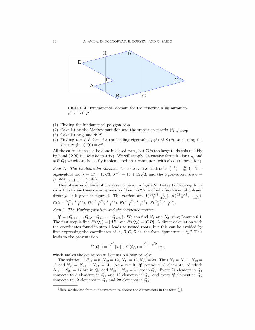
30 A. AVILA, D. DOLGOPYAT, E. DURYEV, AND O. SARIG
AC
E
D
B
F
G
H
Figure 4. Fundamental domain for the renormalizing automor-phism of
√2
(1) Finding the fundamental polygon of φ(2) Calculating the Markov partition and the transition matrix (tPQ)P×P(3) Calculating g and Ψ(θ)(4) Finding a closed form for the leading eigenvalue µ(θ) of Ψ(θ), and using the
identity (lnµ)′′(0) = σ2.
All the calculations can be done in closed form, but P is too large to do this reliablyby hand (Ψ(θ) is a 58×58 matrix). We will supply alternative formulas for tPQ andg(P,Q) which can be easily implemented on a computer (with absolute precision).
Step 1. The fundamental polygon. The derivative matrix is(
11 −42−6 23
). The
eigenvalues are λ = 17 − 12√
2, λ−1 = 17 + 12√
2, and the eigenvectors are v =(1−2√
21
)and w =
(1+2√
21
).1
This places us outside of the cases covered in figure 2. Instead of looking for areduction to one these cases by means of Lemma 2.7, we find a fundamental polygon
directly. It is given in figure 4. The vertices are A( 4+√
28 , 1
4√
2), B( 12−
√2
8 ,− 14√
2),
C(2 + 7√
28 , 4−
√2
8 ), D( 12+√
28 , 8+
√2
8 ), E( 4−√
28 , 8−
√2
8 ), F ( 7√
28 , 4−
√2
8 ).
Step 2. The Markov partition and the incidence matrix
P = Q11, . . . , Q1N1;Q21, . . . , Q2N2
. We can find N1 and N2 using Lemma 6.4.The first step is find `u(Q1) = |AB| and `u(Q2) = |CD|. A direct calculation withthe coordinates found in step 1 leads to nested roots, but this can be avoided byfirst expressing the coordinates of A,B,C,D in the form “puncture + tv.” Thisleads to the presentation
`u(Q1) =
√2
4‖v‖ , `u(Q2) =
2 +√
2
4‖v‖,
which makes the equations in Lemma 6.4 easy to solve.The solution is N11 = 5, N12 = 12, N21 = 12, N22 = 29. Thus N1 = N11 +N12 =
17 and N2 = N21 + N22 = 41. As a result, P contains 58 elements, of whichN11 +N21 = 17 are in Q1 and N12 +N22 = 41 are in Q2. Every P–element in Q1
connects to 5 elements in Q1 and 12 elements in Q2; and every P-element in Q2
connects to 12 elements in Q1 and 29 elements in Q2.
1Here we deviate from our convention to choose the eigenvectors in the form(1∗).
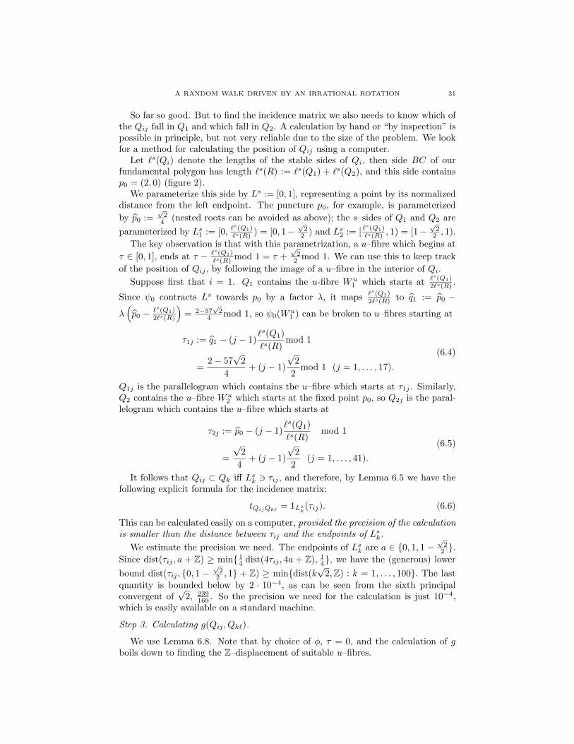
A RANDOM WALK DRIVEN BY AN IRRATIONAL ROTATION 31
So far so good. But to find the incidence matrix we also needs to know which ofthe Qij fall in Q1 and which fall in Q2. A calculation by hand or “by inspection” ispossible in principle, but not very reliable due to the size of the problem. We lookfor a method for calculating the position of Qij using a computer.
Let `s(Qi) denote the lengths of the stable sides of Qi, then side BC of ourfundamental polygon has length `s(R) := `s(Q1) + `s(Q2), and this side containsp0 = (2, 0) (figure 2).
We parameterize this side by Ls := [0, 1], representing a point by its normalizeddistance from the left endpoint. The puncture p0, for example, is parameterized
by p0 :=√
24 (nested roots can be avoided as above); the s–sides of Q1 and Q2 are
parameterized by Ls1 := [0, `s(Q1)`s(R) ) = [0, 1−
√2
2 ) and Ls2 := [ `s(Q1)`s(R) , 1) = [1−
√2
2 , 1).
The key observation is that with this parametrization, a u–fibre which begins at
τ ∈ [0, 1], ends at τ − `s(Q1)`s(R) mod 1 = τ +
√2
2 mod 1. We can use this to keep track
of the position of Qij , by following the image of a u–fibre in the interior of Qi.
Suppose first that i = 1. Q1 contains the u-fibre Wu1 which starts at `s(Q1)
2`s(R) .
Since ψ0 contracts Ls towards p0 by a factor λ, it maps `s(Q1)2`s(R) to q1 := p0 −
λ(p0 − `s(Q1)
2`s(R)
)= 2−57
√2
4 mod 1, so ψ0(Wu1 ) can be broken to u–fibres starting at
τ1j := q1 − (j − 1)`s(Q1)
`s(R)mod 1
=2− 57
√2
4+ (j − 1)
√2
2mod 1 (j = 1, . . . , 17).
(6.4)
Q1j is the parallelogram which contains the u–fibre which starts at τ1j . Similarly,Q2 contains the u–fibre Wu
2 which starts at the fixed point p0, so Q2j is the paral-lelogram which contains the u–fibre which starts at
τ2j := p0 − (j − 1)`s(Q1)
`s(R)mod 1
=
√2
4+ (j − 1)
√2
2(j = 1, . . . , 41).
(6.5)
It follows that Qij ⊂ Qk iff Lsk 3 τij , and therefore, by Lemma 6.5 we have thefollowing explicit formula for the incidence matrix:
tQijQk` = 1Lsk(τij). (6.6)
This can be calculated easily on a computer, provided the precision of the calculationis smaller than the distance between τij and the endpoints of Lsk.
We estimate the precision we need. The endpoints of Lsk are a ∈ 0, 1, 1−√
22 .
Since dist(τij , a + Z) ≥ min 14 dist(4τij , 4a + Z), 1
4, we have the (generous) lower
bound dist(τij , 0, 1 −√
22 , 1 + Z) ≥ mindist(k
√2,Z) : k = 1, . . . , 100. The last
quantity is bounded below by 2 · 10−4, as can be seen from the sixth principalconvergent of
√2, 239
169 . So the precision we need for the calculation is just 10−4,which is easily available on a standard machine.
Step 3. Calculating g(Qij , Qk`).
We use Lemma 6.8. Note that by choice of φ, τ = 0, and the calculation of gboils down to finding the Z–displacement of suitable u–fibres.
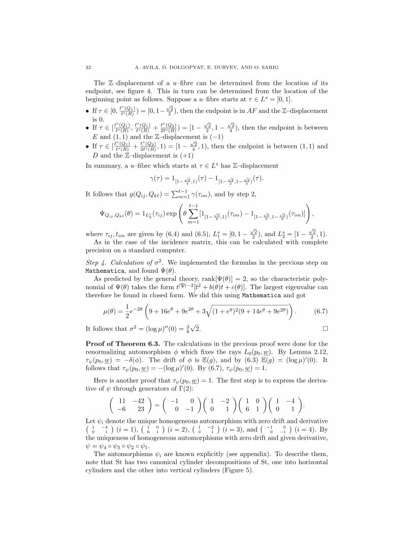
32 A. AVILA, D. DOLGOPYAT, E. DURYEV, AND O. SARIG
The Z–displacement of a u–fibre can be determined from the location of itsendpoint, see figure 4. This in turn can be determined from the location of thebeginning point as follows. Suppose a u–fibre starts at τ ∈ Ls = [0, 1].
• If τ ∈ [0, `s(Q1)`s(R) ) = [0, 1−
√2
2 ), then the endpoint is in AF and the Z–displacement
is 0.• If τ ∈ [ `
s(Q1)`s(R) ,
`s(Q1)`s(R) + `s(Q2)
2`s(R) ) = [1 −√
22 , 1 −
√2
4 ), then the endpoint is between
E and (1, 1) and the Z–displacement is (−1)
• If τ ∈ [ `s(Q1)`s(R) + `s(Q2)
2`s(R) , 1) = [1 −√
24 , 1), then the endpoint is between (1, 1) and
D and the Z–displacement is (+1)
In summary, a u–fibre which starts at τ ∈ Ls has Z–displacement
γ(τ) = 1[1−
√2
4 ,1)(τ)− 1
[1−√
22 ,1−
√2
4 )(τ).
It follows that g(Qij , Qk`) =∑`−1m=1 γ(τim), and by step 2,
ΨQij ,Qk`(θ) = 1Lsk(τij) exp
(θ
`−1∑m=1
[1[1−
√2
4 ,1)(τim)− 1
[1−√
22 ,1−
√2
4 )(τim)]
),
where τij , tim are given by (6.4) and (6.5), Ls1 = [0, 1−√
22 ), and Ls2 = [1−
√2
2 , 1).As in the case of the incidence matrix, this can be calculated with complete
precision on a standard computer.
Step 4. Calculation of σ2. We implemented the formulas in the previous step onMathematica, and found Ψ(θ).
As predicted by the general theory, rank[Ψ(θ)] = 2, so the characteristic poly-nomial of Ψ(θ) takes the form t|P|−2[t2 + b(θ)t+ c(θ)]. The largest eigenvalue cantherefore be found in closed form. We did this using Mathematica and got
µ(θ) =1
2e−2θ
(9 + 16eθ + 9e2θ + 3
√(1 + eθ)2(9 + 14eθ + 9e2θ)
). (6.7)
It follows that σ2 = (logµ)′′(0) = 38
√2.
Proof of Theorem 6.3. The calculations in the previous proof were done for therenormalizing automorphism φ which fixes the rays L0(p0, w). By Lemma 2.12,τψ(p0, w) = −δ(φ). The drift of φ is E(g), and by (6.3) E(g) = (logµ)′(0). Itfollows that τψ(p0, w) = −(logµ)′(0). By (6.7), τψ(p0, w) = 1.
Here is another proof that τψ(p0, w) = 1. The first step is to express the deriva-tive of ψ through generators of Γ(2):(
11 −42−6 23
)=
(−1 0
0 −1
)(1 −20 1
)(1 06 1
)(1 −40 1
).
Let ψi denote the unique homogeneous automorphism with zero drift and derivative(1 −40 1
)(i = 1),
(1 06 1
)(i = 2),
(1 −20 1
)(i = 3), and
( −1 00 −1
)(i = 4). By
the uniqueness of homogeneous automorphisms with zero drift and given derivative,ψ = ψ4 ψ3 ψ2 ψ1.
The automorphisms ψi are known explicitly (see appendix). To describe them,note that St has two canonical cylinder decompositions of St, one into horizontalcylinders and the other into vertical cylinders (Figure 5).
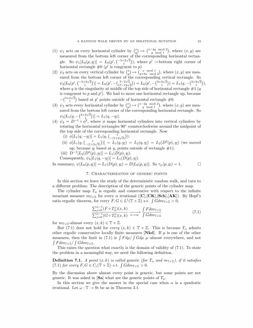
A RANDOM WALK DRIVEN BY AN IRRATIONAL ROTATION 33
(1) ψ1 acts on every horizontal cylinder by(xy
)7→(x−4y mod 2y mod 1
), where (x, y) are
measured from the bottom left corner of the corresponding horizontal rectan-
gle. So ψ1[L0(p, w)] = L0(p′,(−3+2
√2
1
)), where p′ :=bottom right corner of
horizontal rectangle #0 (p′ is congruent to p)
(2) ψ2 acts on every vertical cylinder by(xy
)7→(
x mod 1y+6x mod 2
), where (x, y) are mea-
sured from the bottom left corner of the corresponding vertical rectangle. So
ψ2[L0(p′,(−3+2
√2
1
))] = L0(p′,−
( 3−2√
217−12
√2
)) = L0(p′,−
(3+2√
21
)) = L1(q,−
(3+2√
21
)),
where q is the singularity at middle of the top side of horizontal rectangle #1 (qis congruent to p and p′). We had to move one horizontal rectangle up, because
−(
3+2√
21
)based at p′ points outside of horizontal rectangle #0.
(3) ψ3 acts every horizontal cylinder by(xy
)7→(x−2y mod 2y mod 1
), where (x, y) are mea-
sured from the bottom left corner of the corresponding horizontal rectangle. So
ψ3[L1(q,−(
3+2√
21
))] = L1(q,−w).
(4) ψ4 = D−1 φ2, where φ maps horizontal cylinders into vertical cylinders byrotating the horizontal rectangles 90 counterclockwise around the midpoint ofthe top side of the corresponding horizontal rectangle. Now
(i) φ[L1(q,−w)] = L1(q,(
1−(1+2
√2)
));
(ii) φ[L1(q,(
1−(1+2
√2)
))] = L1(q, w) = L2(q, w) = L2(D2(p), w) (we moved
up, because w based at q, points outside of rectangle #1);(iii) D−1[L2(D2(p), w)] = L1(D(p), w).Consequently, ψ4[L1(q,−w)] = L1(D(p), w).
In summary, ψ[L0(p, w)] = L1(D(p), w) = D[L0(p, w)]. So τψ(p, w) = 1.
7. Characterization of generic points
In this section we leave the study of the deterministic random walk, and turn toa different problem: The description of the generic points of the cylinder map.
The cylinder map Tα is ergodic and conservative with respect to the infiniteinvariant measure mT×Z for every α irrational ([C],[CK],[Sch],[AK]). By Hopf’sratio ergodic theorem, for every F,G ∈ L1(T× Z) s.t.
∫GdmT×Z > 0,∑n−1
j=0 (F T jα)(x, k)∑n−1j=0 (G T jα)(x, k)
−−−−→n→∞
∫FdmT×Z∫GdmT×Z
(7.1)
for mT×Z-almost every (x, k) ∈ T× Z.But (7.1) does not hold for every (x, k) ∈ T × Z. This is because Tα admits
other ergodic conservative locally finite measures [Nkd]. If µ is one of the othermeasures, then the limit in (7.1) is
∫Fdµ/
∫Gdµ µ–almost everywhere, and not∫
FdmT×Z/∫GdmT×Z.
This raises the question what exactly is the domain of validity of (7.1). To statethe problem in a meaningful way, we need the following definition.
Definition 7.1. A point (x, k) is called generic (for Tα and mT×Z), if it satisfies(7.1) for every F,G ∈ Cc(T× Z) s.t.
∫GdmT×Z > 0.
By the discussion above almost every point is generic, but some points are notgeneric. It was asked in [Sa] what are the generic points of Tα.
In this section we give the answer in the special case when α is a quadraticirrational. Let ω : T→ St be as in Theorem 3.1.
34 A. AVILA, D. DOLGOPYAT, E. DURYEV, AND O. SARIG
Theorem 7.2. Suppose α is a quadratic irrational, with renormalizing automor-phism ψ, then (x, k) is generic for Tα and mT×Z iff 1
nξ[ψn(ω(x))] −−−−→
n→∞0.
Let(
sin θcos θ
)denote the stable direction of ψ, and ϕθ the linear flow in direction θ on
the infinite staircase. A point ω ∈ St is called generic for ϕθ and the area measure
m, if∫ T
0F [ϕtθ(ω)]dt/
∫ T0G[ϕtθ(ω)]dt −−−−→
T→∞
∫Fdm/
∫Ggm for every F,G ∈ Cc(St)
s.t.∫Gdm > 0. We will obtain Theorem 7.2 from the following result.
Theorem 7.3. ω ∈ St is generic for ϕθ and m iff 1k ξ[ψ
k(ω)] −−−−→k→∞
0.
Theorem 7.2 follows from Theorem 7.3 in the same way Theorem 3.1 follows fromTheorem 3.2.
Proof of Theorem 7.3. If the theorem holds for one choice of a Z–coordinate,then it works for all choices of Z–coordinates, therefore we are free to use theZ–coordinate of our choice. We choose the Z–coordinate associated to ψ.
Suppose ξ[ψk(ω0)]/k −−−−→k→∞
0, then ω0 is generic because of Theorem 3.2 : the
fluctuating exponential term cancels out upon division.The remainder of the proof deals with the implication “genericity⇒zero drift.”
We use the strategy of [SS].Fix a generic point ω0 ∈ St, let AT := ϕtθ(ω0) : 0 ≤ t ≤ T, and define λT to be
the normalized length measure on AT ∩ [ξ = 0]. Since ω0 is generic, λT convergesweak star to the normalized Lebesgue measure on [ξ = 0].
Construction: Fix some N ≥ 1 to be chosen later, and define for every k ≥ 0
XNk := ξ ψ(k+1)N − ξ ψkN =
((k+1)N−1∑j=kN
Fψ ψj0) π.
We think of XNk as of bounded random variables on (AT ,B(AT ), λT ). The bound
is |XNk | ≤ N max |Fψ|.
Let log∗ := logλ−1 , where λ is the eigenvalue of the derivative of ψ in (0, 1).Since ξ = 0 λT –a.e. and Fψ is uniformly bounded,
1N [log∗ T ]−2∑
k=0
XNk =
1N [log∗ T ]−1∑
k=0
XNk +O(N) = ξ ψ[log∗ T ] − ξ +O(N)
= ξ ψ[log∗ T ] +O(N) uniformly on supp(λT ).
The right hand side is nearly constant λT –a.s., because ψ[log∗ T ] contracts the sup-port of λT (a subset of AT ) to a set of diameter less than λ−1, and the Z–coordinatesof points in such a set must be uniformly bounded away from one another. It followsthat for λT –a.e. ω ∈ AT ,
1N [log∗ T ]−2∑
k=0
XNk (ω) = ξ[ψ[log∗ T ](ω0)] +O(N) uniformly in T .
Taking expectations with respect to λT and dividing by [log∗ T ], we obtain
ξ[ψ[log∗ T ](ω0)]
[log∗ T ]= EλT
1
[log∗ T ]
1N [log∗ T ]−2∑
k=0
XNk
+ o(1), as T →∞. (7.2)
A RANDOM WALK DRIVEN BY AN IRRATIONAL ROTATION 35
The expectation of 1[log∗ T ]
∑ 1N [log∗ T ]−2
k=0 XNk with respect to the normalized Lebes-
gue’s measure on [ξ = 0] is zero (because ψ is an automorphism with zero drift).
We will use the genericity (in the form λTw∗−−−−→
T→∞Normalized Lebesgue[ξ=0]) to
show that something close happens to the λT –expectation. More precisely:
Claim. If ω0 is generic then for every ε there exists N s.t. for all T large enough
max|EλT ( 1
NXNk )| : 0 ≤ k ≤ 1
N [log∗ T ]− 2< ε. (7.3)
Together with (7.2), this implies that 1k ξk(ω0) −−−−→
k→∞0 and finishes the proof.
We begin the proof of (7.3). Fix ω0 generic and ε > 0, and let C, δ0, N0 besome parameters that will be calibrated at the end of the proof. Let λCT denote thelength measure on AT ∩ [|ξ| ≤ C], normalized so that λCT [ξ = 0] = 1 (this is not aprobability measure).
Step 1. Choosing N > N0 and τ s.t. λCT[| 1NX
N0 | > δ0
]< δ0 for all T > τ .
Proof. Fix 0 < δ < δ0. Since 1k ξ ψ
k −−−−→k→∞
0 almost everywhere with respect to
Lebesgue’s measure, we can use Egoroff’s theorem to find N = N(δ, C) > N0 s.t.Λ0 := ω ∈ St : |ξ(ω)| ≤ C, | 1
NXN0 | > δ0 satisfies m(Λ0) < δ, where m is the area
measure on St.Since ω0 is generic, λCT converges w∗ to the Lebesgue measure on [|ξ| ≤ C]. The
indicator functions of Λ0 and [ξ = 0] are discontinuous, but all discontinuities lieon the boundaries of the parallelograms of the Markov partition, and their imagesunder ψ−N . N is fixed, therefore the closure of the singular set has measure zero.Using a standard approximation argument, it is easy to show that λCT (Λ0) −−−−→
T→∞m(Λ0) < δ. It follows that there exists τ = τ(δ, C) s.t. for all T > τ(δ, C),λCT (Λ0) < δ, proving step 1.
Step 1 allows us to bound EλT ( 1NX
N0 ) as follows. Choose δ0 < ε/(1 + max |Fψ|),
then for all T > τ ,
|EλT ( 1NX
N0 )| ≤ δ0 + max | 1
NXN0 | · λT
[| 1NX
N0 | ≥ δ0
]≤ δ0(1 + max |Fψ|) < ε.
It is tempting to try to bound EλT ( 1NX
Nk ) for k 6= 0 in the same way. Unfortu-
nately the methods of step 1 can only be used for bounded k, whereas (7.3) callsfor a uniform bound for 0 ≤ k ≤ [log∗ T ], as T →∞.
We will take an indirect approach. Imagine we were able to construct self mapsθk : AT → AT (0 ≤ k ≤ 1
N [log∗ T ]− 2) with the following properties:
• XNk = XN
0 θk+error, uniformly bounded by E0,• θk is Borel, one-to-one, and θk(AT ∩ [ξ = 0]) ⊂ AT ∩ [|ξ| ≤ C],
• C−1r ≤ d`θk
d` ≤ Cr where d` is the (Lebesgue) length measure and Cr is a globalconstant, independent of N,T, k, and ε.
Then it would follow that λT ≤ CrλCT θk|[ξ=0], and if E0/N0 < δ0 then
λT [| 1NX
Nk | > 2δ0] ≤ Cr(λCT θk)([| 1
NXNk | > 2δ0] ∩ [ξ = 0])
≤ CrλCT [| 1NX
Nk θ−1
k | > δ0] ≤ CrλCT [| 1NX
N0 | > δ0] < Crδ0.
This, and the fact that sup |XNk | are uniformly bounded, is sufficient to bound
EλT (| 1NX
Nk |) uniformly and prove (7.3).
36 A. AVILA, D. DOLGOPYAT, E. DURYEV, AND O. SARIG
In reality we do not know how to construct such θk, because of edge effects atthe endpoints of AT . Luckily these edge effects can be controlled well enough topush this argument through with minor modifications. The details follow.
Step 2. Breaking AT into the “interior” and “edge” s–fibres.
We use the Adler–Weiss coding of Theorem 2.8 and Lemma 3.3. Recall that an s–fibre is a set of the form W s(x, k) :=lift to [ξ = k] of W s(x) := π0(y) : y∞0 = x∞0 ,where z∞0 := (z0, z1, . . .). This is a stable linear segment, with length h(x0).
We define an n0–stable block to be the lift to [ξ = k] of a set of the formπ0(y) : y∞−n0
= x∞−n0. These are closed stable linear segments, and their length is
λn0h(x−n0) λn0 −−−−→n0→∞
0. (An Bn means C−1 < An/Bn < C for all n large.)
Different n0–stable blocks are disjoint, or they meet at one or two endpoints. Everypoint belongs to at most two n0–stable blocks.BT := ψ[log∗ T ](AT ) is a stable linear segment with length in [1, λ−1]. The n0–
stable blocks which intersect the relative interior of BT fall into two groups:
• two or less “edge” n0–stable blocks which cover the endpoints of BT ;• (1− 4λn0 maxh)/(λn0 minh) or more “interior” n0–stable blocks which lie com-
pletely inside BT .
Since the number of interior n0–blocks tends to infinity as n0 → ∞, it is possibleto fix once and for all n0 in such a way that there is at least one interior block.
This choice is independent of N0, therefore it is possible to assume without lossof generality that N0 > n0.
If [log∗ T ] n0, then the decomposition of BT = ψ[log∗ T ](AT ) into interior andboundary n0–blocks induces a decomposition of AT into interior and edge s–fibres.Here and throughout:
• An edge s–fibre of AT is an s–fibre in ψ−[log∗ T ](edge n0–block of BT ).• An interior s–fibre of AT is a stable fibre in ψ−[log∗ T ](interior n0–block of BT ).
Let Wint,Wbnd be the collection of interior and edge stable fibres in AT . The interiorof AT is AT (int) :=
⋃Wint, and the boundary of AT is AT (bnd) :=
⋃Wbnd.
Step 3. Defining θk on AT (int) (0 ≤ k ≤ 1N [log∗ T ]− 2).
Recall that G is the dynamical graph of the Markov partition P. An admissibleword is a finite word w0 · · ·wn ∈ Pn s.t. w0 → · · · → wn is a path on G .
Since Σ(G ) is topologically mixing, there exists a constant Mbr such that forevery pair of a, b ∈ P there is a path wab on G of length Mbr s.t. awabb is admissible.Fix for such a, b a word wab, and call it the bridge from a to b. In what follows
(a,bridge, b) := (a,walastbfirst, b).
We define θk : AT (int)→ AT as follows. Suppose ω ∈ AT (int). Fix a stable fibreW s(x, η) ⊂ AT (int). All but countably many points in W s(x, η) can be uniquelyrepresented in the form (y, η) where
y ∈ Σ(G ) , y∞0 = x∞0 , ξ(ω) = η, and π(ω) = π0(y).
A RANDOM WALK DRIVEN BY AN IRRATIONAL ROTATION 37
Write y = (y−1−∞|B0, B1, . . . , Bk, y
∞kN ), where Bi are words of length of N , and the
zeroth coordinate is to the immediate right of |. We let θk(y, η) := (z, η′) where
z = σ4Mbr (y−1−∞|bridge, Bk,bridge, B1, . . . , Bk−1,bridge, B0,bridge, y∞(k+1)N )
η′ = η +
[log∗ T ]−1∑j=0
F (σjy)− F (σjz), where F := Fψ π0.
What we have done here is to exchange block zero with block k, plug-in bridge wordsto ensure admissibility, and at the end apply the shift and modify η to ensure thatwe remain inside AT (see below). Here are some properties of θk.
(i) XN0 θk = XN
k +bounded error: θk exchanges the zeroth block with the k–thblock, and therefore |XN
0 θk −XNk | ≤ 6Mbr max |Fψ|. Here we are using (2.4).
(ii) θk[AT (int)] ⊂ AT (int) for all 0 ≤ k ≤ 1N [log∗ T ]−2: We abuse notation and
identify a point in St with its symbolic coding in Σ(G )×Z. Suppose (y, η) belongs
to an interior n0–block and 0 ≤ k ≤ 1N [log∗ T ]− 2, then
(σ[log∗ T ]z)∞−N = σ[log∗ T ](y)∞−N , because of the σ4Mbr in the definition of z, and
ψ[log∗ T ](z, η′) =(σ[log∗ T ](z), η′ +
[log∗ T ]−1∑j=0
F (σjz))
=(σ[log∗ T ](z), η +
[log∗ T ]−1∑j=0
F (σjy)), by the definition of η′.
Since N > n0, ψ[log∗ T ](z, η′) belongs to the same n0–block which containsψ[log∗ T ](y, η). This is an interior n0–block of BT = ψ[log∗ T ](AT ). So (z, η′) ∈ AT .
(iii) θk[supp(λT )] ⊂ supp(λC′
T ) for C ′ := 100[Mbr + 1] max |Fψ|: It is enough
to check that |η′ − η| =∣∣∣∑[log∗ T ]−1
j=0 F (σjz)−∑[log∗ T ]−1j=0 F (σjy)
∣∣∣ ≤ C ′. To check
this we recall that F is constant on symbolic 2–cylinders, therefore the differencebetween the two sums can only come from the following sources:
– the effect of the shift by σ4Mbr , bounded by 2 · 4Mbr max |Fψ|– the sum over the bridge words, bounded by 4Mbr max |Fψ|– the value of F (σjz) for the j at the end of Bk, Bk−1, and B0, with a total
effect bounded by 3 max |Fψ|This gives the bound above with C much smaller than claimed.
(iv) θk is one-to-one on AT (int): To reconstruct y from z one just needs to erasethe bridge words (whose position is always the same), and then exchange the k–thblock with the zeroth block of what remains. Once y is known, η can be easilycalculated from η′ and z.
(v) d`θk/d` is uniformly bounded away from 0,∞, where ` is the length measureon AT : For every a ∈ Σ(G ), the length of the stable linear segment
[a∞−n] := ω ∈ AT (int) ∩ [ξ = 0] : π(ω) = π0(y), yj = aj (j ≥ −n)
is λnh(a−n), because ψ−n[a∞−n] = W s(σ−na), `[W s(σ−na)] = h(a−n), and ψ−n
expands linear stable segments by a factor of λ−n. With this formula at hand, it iseasy to see that d`θk
d` ∈ [λ4Mbr ( minhmaxh ), λ4Mbr (maxh
minh )].
38 A. AVILA, D. DOLGOPYAT, E. DURYEV, AND O. SARIG
Step 4. Defining θk on A(bnd).
Fix once and for all an interior stable fibre W s(x, η) of AT . We will define θk onan edge stable fibre by first mapping it into W s(x, η), and then applying θk|A(int)
as defined in step 3.The resulting transformation is θk : (y, η) 7→ (z, η′) where
z = σ5Mbr (y−1−∞|bridge, Bk,bridge, B1, . . . , Bk−1,bridge, B0,bridge,
y[log∗ T ]−1kN ,bridge, x∞[log∗ T ])
η′ = η +
[log∗ T ]∑j=0
Fψ(σjy)− Fψ(σjz)
The following properties can be verified as in the previous step:
(i) XN0 θk = XN
k +bounded error. The error is bounded by 8Mbr max |Fψ|.(ii) θk[A(bnd)] ⊂ AT (int) and θk[A(bnd)]∩ [ξ = 0]) ⊂ AT (bnd)∩ [|ξ| ≤ C ′] with
C ′ as above.(iii) θk is one-to-one on each boundary stable fibre, and its Radon-Nikodym
derivative takes values in [λ5Mbr ( minhmaxh ), λ5Mbr (maxh
minh )].
Step 5. Proof of (7.3).
We estimate EλT ( 1NX
Nk ) for 0 ≤ k ≤ 1
N [logλ−1 T ]−2. Since |XNk | ≤ N max |Fψ|,∣∣EλT ( 1
NXNk )∣∣ ≤ 2δ0 + max |Fψ| · λT (Λk), (7.4)
where Λk := ω ∈ S : ξ(ω) = 0, | 1NX
Nk | > 2δ0. We will bound λT (Λk).
We now choose the constants C,N0, δ0: C := C ′ = 100(Mbr + 1) max |Fψ|,δ0 := ε/(2 + 3λ−5Mbr
(maxhminh
)max |Fψ|), and N0 so large that
10Mbr max |Fψ|N0
< δ0.
By construction, |XNk −XN
0 θk| ≤ 8Mbr max |Fψ|, so if | 1NX
Nk (ω)| > 2δ0 then
| 1NX
N0 (θk(ω))| > 2δ0 − 10Mbr max |Fψ|
N0> δ0. We see that
θk(Λk) ⊂ ω ∈ AT : |ξ(ω)| ≤ C, | 1NX
N0 | > δ0.
Applying θ−1k to both sides and recalling that θk is piecewise invertible, at worst
three-to-one (edge effects), and d`θkd` ≥ λ
5Mbr ( minhmaxh ) we find that
λT (Λk) ≤ 3λ−5Mbr(
maxhminh
)λCT[| 1NX
N0 | > δ0
].
By step 1, λT (Λk) ≤ 3λ−5Mbr(
maxhminh
)δ0. Substituting this at (7.4) we find that∣∣EλT ( 1
NXNk )∣∣ ≤ δ0(2 + 3λ−5Mbr
(maxhminh
)max |Fψ|) < ε as required.
Appendix A. Proofs of Proposition 2.3, Lemma 2.7, and Lemma 2.9
Classification of homogeneous automorphisms. We prove Proposition 2.3:
(1) If A ∈ SL(2,Z), A =(
1 00 1
)mod 2 and δ0 ∈ Z, then there is a unique homo-
geneous automorphism with derivative A and drift δ0.(2) If A ∈ SL(2,Z), A =
(0 1
−1 0
)mod 2 and δ0 ∈ 1
2 + Z, then there is a uniquehomogeneous automorphism with derivative A and drift δ0.
(3) No other homogeneous automorphisms exist.

A RANDOM WALK DRIVEN BY AN IRRATIONAL ROTATION 39
Step 1. Existence of homogeneous automorphisms as in parts 1 and 2.
Proof. Let Γ(2) := A ∈ SL(2,Z) : A =(
1 00 1
)mod 2, Γ := Γ(2)∪
(0 1
−1 0
)Γ(2).
Γ(2) is generated by(
1 20 1
),(
1 02 1
), and
( −1 00 −1
). We will construct
• A homogeneous automorphism with derivative(
1 00 1
)and drift +1;
• A homogeneous automorphism with derivative(
1 20 1
)and drift 0;
• A homogeneous automorphism with derivative(
1 02 1
)and drift 0;
• A homogeneous automorphism with derivative( −1 0
0 −1
)and drift 0;
• A homogeneous automorphism with derivative(
0 −11 0
)and drift 1
2 .
The automorphisms in part (1) can be constructed from the first three automor-phisms. The automorphisms in part (2) require an additional composition with thefourth automorphism.
A homogeneous automorphism with derivative(
1 00 1
)and drift 1: D.
A homogeneous automorphism with derivative(
1 20 1
)and drift 0: Divide St into
horizontal cylinders, as indicated by the dashed lines in figure 5(a). Act on eachcylinder by the map (x, y) 7→ (x+ 2y mod 2, y) up to identifications, where (x, y)are measured relative to the bottom left corner. These maps equal the identity onthe boundary of the cylinder (the horizontal sides of the rectangle), therefore they
glue to an automorphism ψ. The derivative of ψ is(
1 20 1
), ψ commutes with D,
and ψ fixes the singularities of St. It has zero drift, because the Frobenius functionwith respect to the horizontal rectangles vanishes.
A homogeneous automorphism with derivative(
1 02 1
)and drift 0: The same con-
struction, but using the decomposition of St into vertical cylinders (figure 5(a)).
A homogeneous automorphism with derivative(
0 −11 0
)and drift 1
2 : DecomposeSt into hotizontal rectangles. Rotate every rectangle 90 degrees counterclockwisearound the midpoint of its top side, turning it into a vertical rectangle. These mapsglue continuously to an automorphism of St (figure 5(b)). Using the Z–coordinatedefined by the horizontal rectangles, one sees that the average drift is 1
2 .
A homogeneous automorphism with derivative( −1 0
0 −1
)and drift 0: Suppose ψ
is the automorphism with drift 12 and derivative
(0 1
−1 0
)constructed above, then
ϕ := D−1 ψ2 has zero drift and derivative( −1 0
0 −1
).
Step 2. A homogeneous automorphism with derivative(
1 00 1
)is equal to Dk for
some k ∈ Z. Two homogeneous automorphisms with the same derivative and driftare equal.
Proof. Let ψ be a homogeneous automorphism with derivative(
1 00 1
). Fix a
horizontal rectangle R and let p0 denote the singularity at its lower right corner.Given p ∈ int(R), let γp ⊂ R denote the linear segment from p0 to p. Since ψ fixesthe D–orbit of p0, ψ[γp] is a linear segment from p0 or D(p0) to ψ(p). Since the
derivative of ψ is(
1 00 1
), ψ[γp] has the same slope, length, and direction as γp.
There are infinitely many such segments, one for every horizontal rectangleDk(R), k ∈ Z. By reasons of continuity there is some fixed k ∈ Z such thatψ[γp] ⊂ Dk(R) for all p ∈ int(R). It follows that ψ = Dk on R. Since ψ commuteswith D, ψ = Dk on St. This proves the first part of step 2.
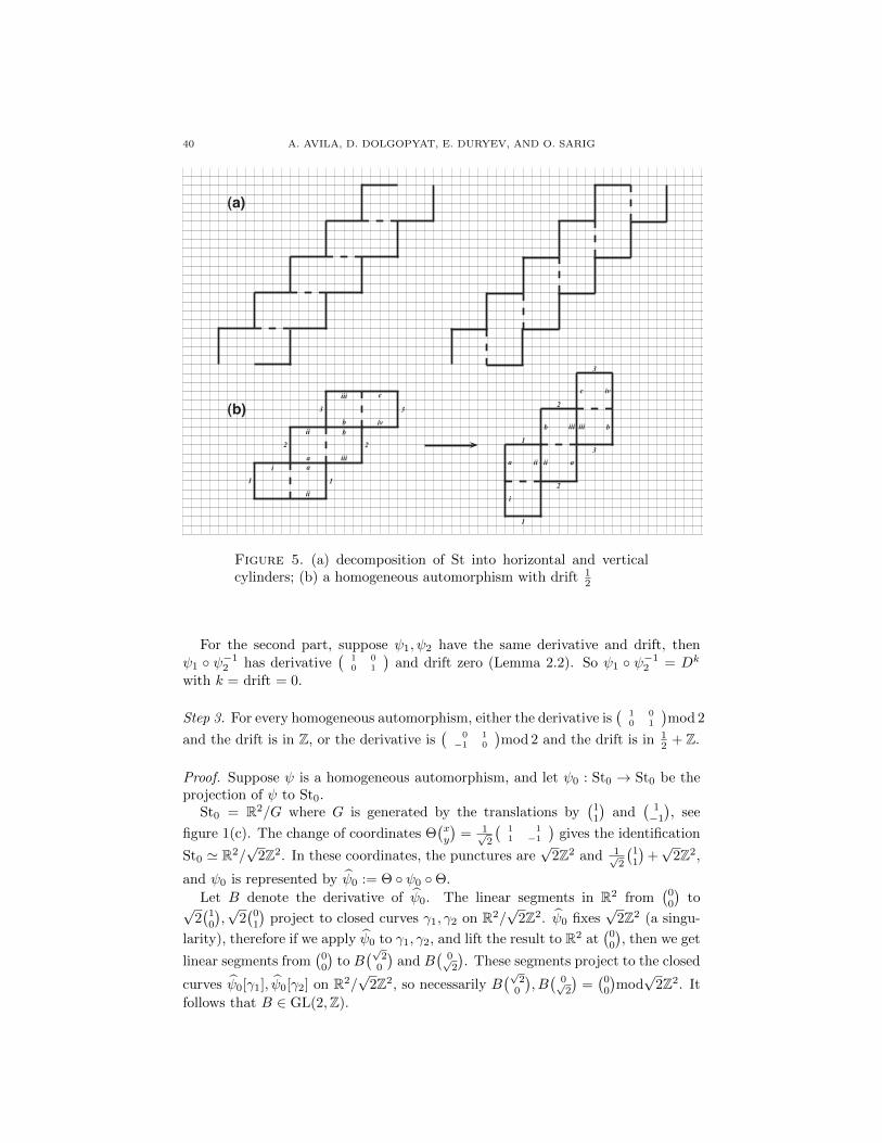
40 A. AVILA, D. DOLGOPYAT, E. DURYEV, AND O. SARIG
(a)
(b)
1
2
3
1
2
3
1
2
3 1
2
3
i
iv ii
ii
iii
iii
iv
ii ii
iii iii
i
aa
c
bb
a a
b b
c
Figure 5. (a) decomposition of St into horizontal and verticalcylinders; (b) a homogeneous automorphism with drift 1
2
For the second part, suppose ψ1, ψ2 have the same derivative and drift, thenψ1 ψ−1
2 has derivative(
1 00 1
)and drift zero (Lemma 2.2). So ψ1 ψ−1
2 = Dk
with k = drift = 0.
Step 3. For every homogeneous automorphism, either the derivative is(
1 00 1
)mod 2
and the drift is in Z, or the derivative is(
0 1−1 0
)mod 2 and the drift is in 1
2 + Z.
Proof. Suppose ψ is a homogeneous automorphism, and let ψ0 : St0 → St0 be theprojection of ψ to St0.
St0 = R2/G where G is generated by the translations by(
11
)and
(1−1
), see
figure 1(c). The change of coordinates Θ(xy
)= 1√
2
(1 11 −1
)gives the identification
St0 ' R2/√
2Z2. In these coordinates, the punctures are√
2Z2 and 1√2
(11
)+√
2Z2,
and ψ0 is represented by ψ0 := Θ ψ0 Θ.
Let B denote the derivative of ψ0. The linear segments in R2 from(
00
)to√
2(
10
),√
2(
01
)project to closed curves γ1, γ2 on R2/
√2Z2. ψ0 fixes
√2Z2 (a singu-
larity), therefore if we apply ψ0 to γ1, γ2, and lift the result to R2 at(
00
), then we get
linear segments from(
00
)to B
(√2
0
)and B
(0√2
). These segments project to the closed
curves ψ0[γ1], ψ0[γ2] on R2/√
2Z2, so necessarily B(√
20
), B(
0√2
)=(
00
)mod√
2Z2. It
follows that B ∈ GL(2,Z).
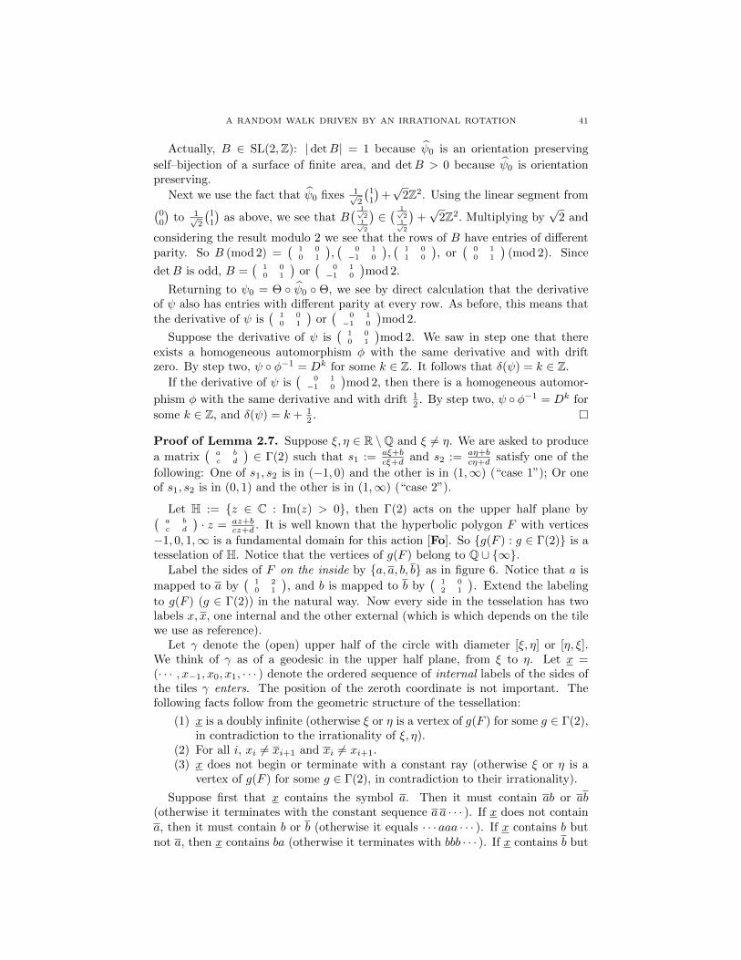
A RANDOM WALK DRIVEN BY AN IRRATIONAL ROTATION 41
Actually, B ∈ SL(2,Z): |detB| = 1 because ψ0 is an orientation preserving
self–bijection of a surface of finite area, and detB > 0 because ψ0 is orientationpreserving.
Next we use the fact that ψ0 fixes 1√2
(11
)+√
2Z2. Using the linear segment from(00
)to 1√
2
(11
)as above, we see that B
( 1√2
1√2
)∈( 1√
21√2
)+√
2Z2. Multiplying by√
2 and
considering the result modulo 2 we see that the rows of B have entries of differentparity. So B (mod 2) =
(1 00 1
),(
0 1−1 0
),(
1 01 0
), or
(0 10 1
)(mod 2). Since
detB is odd, B =(
1 00 1
)or(
0 1−1 0
)mod 2.
Returning to ψ0 = Θ ψ0 Θ, we see by direct calculation that the derivativeof ψ also has entries with different parity at every row. As before, this means thatthe derivative of ψ is
(1 00 1
)or(
0 1−1 0
)mod 2.
Suppose the derivative of ψ is(
1 00 1
)mod 2. We saw in step one that there
exists a homogeneous automorphism φ with the same derivative and with driftzero. By step two, ψ φ−1 = Dk for some k ∈ Z. It follows that δ(ψ) = k ∈ Z.
If the derivative of ψ is(
0 1−1 0
)mod 2, then there is a homogeneous automor-
phism φ with the same derivative and with drift 12 . By step two, ψ φ−1 = Dk for
some k ∈ Z, and δ(ψ) = k + 12 .
Proof of Lemma 2.7. Suppose ξ, η ∈ R \Q and ξ 6= η. We are asked to produce
a matrix(a bc d
)∈ Γ(2) such that s1 := aξ+b
cξ+d and s2 := aη+bcη+d satisfy one of the
following: One of s1, s2 is in (−1, 0) and the other is in (1,∞) (“case 1”); Or oneof s1, s2 is in (0, 1) and the other is in (1,∞) (“case 2”).
Let H := z ∈ C : Im(z) > 0, then Γ(2) acts on the upper half plane by(a bc d
)· z = az+b
cz+d . It is well known that the hyperbolic polygon F with vertices
−1, 0, 1,∞ is a fundamental domain for this action [Fo]. So g(F ) : g ∈ Γ(2) is atesselation of H. Notice that the vertices of g(F ) belong to Q ∪ ∞.
Label the sides of F on the inside by a, a, b, b as in figure 6. Notice that a is
mapped to a by(
1 20 1
), and b is mapped to b by
(1 02 1
). Extend the labeling
to g(F ) (g ∈ Γ(2)) in the natural way. Now every side in the tesselation has twolabels x, x, one internal and the other external (which is which depends on the tilewe use as reference).
Let γ denote the (open) upper half of the circle with diameter [ξ, η] or [η, ξ].We think of γ as of a geodesic in the upper half plane, from ξ to η. Let x =(· · · , x−1, x0, x1, · · · ) denote the ordered sequence of internal labels of the sides ofthe tiles γ enters. The position of the zeroth coordinate is not important. Thefollowing facts follow from the geometric structure of the tessellation:
(1) x is a doubly infinite (otherwise ξ or η is a vertex of g(F ) for some g ∈ Γ(2),in contradiction to the irrationality of ξ, η).
(2) For all i, xi 6= xi+1 and xi 6= xi+1.(3) x does not begin or terminate with a constant ray (otherwise ξ or η is a
vertex of g(F ) for some g ∈ Γ(2), in contradiction to their irrationality).
Suppose first that x contains the symbol a. Then it must contain ab or ab(otherwise it terminates with the constant sequence a a · · · ). If x does not containa, then it must contain b or b (otherwise it equals · · · aaa · · · ). If x contains b butnot a, then x contains ba (otherwise it terminates with bbb · · · ). If x contains b but
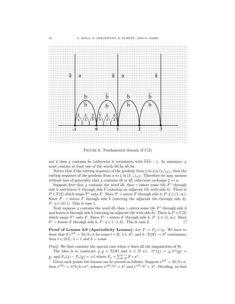
42 A. AVILA, D. DOLGOPYAT, E. DURYEV, AND O. SARIG
0-1 1 2 3
aā a ā ā
b_
b_
b_
bb
bb
bbb_
b_ b
_
aa
aa
āā ā
ā
Figure 6. Fundamental domain of Γ(2)
not a then x contains ba (otherwise it terminates with b b b · · · ). In summary, xmust contain at least one of the words ab, ba, ab, ba.
Notice that if the cutting sequence of the geodesic from ξ to η is (xi)i∈Z, then thecutting sequence of the geodesic from η to ξ is (x−i)i∈Z. Therefore we may assumewithout loss of generality that x contains ab or ab, otherwise exchange ξ ↔ η.
Suppose first that x contains the word ab, then γ enters some tile F ∗ throughside a and leaves it through side b (entering an adjacent tile with side b). There isP ∈ Γ(2) which maps F ∗ onto F . Since P ·γ enters F through side a, P ·ξ ∈ (1,∞).Since P · γ leaves F through side b (entering the adjacent tile through side b),P · η ∈ (0, 1). This is case 1.
Next suppose x contains the word ab, then γ enters some tile F ∗ through side aand leaves it through side b (entering an adjacent tile with side b). There is P ∈ Γ(2)which maps F ∗ onto F . Since P · γ enters F through side a, P · ξ ∈ (1,∞). SinceP · γ leaves F through side b, P · η ∈ (−1, 0). This is case 2.
Proof of Lemma 2.9 (Aperiodicity Lemma). Let F := Fψ π0. We have toshow that if eitF = λh/hσ for some t ∈ R, λ ∈ S1, and h : Σ(G )→ S1 continuous,then t ∈ 2πZ, λ = 1 and h = const.
Proof. We first consider the special case when ψ fixes all the singularities of St.The idea is to construct x, y ∈ Σ(G ) and n ∈ N s.t. σn(x) = x, σn(y) =
y, and Fn(x)− Fn(y) = ±1 where Fn =∑n−1k=0 F σn.
Given such points the lemma can be proved as follows: Suppose eitF = λh/hσ,
then eitFn = λnh/hσn, whence eitFn(x) = λn and eitFn(y) = λn. Dividing, we find
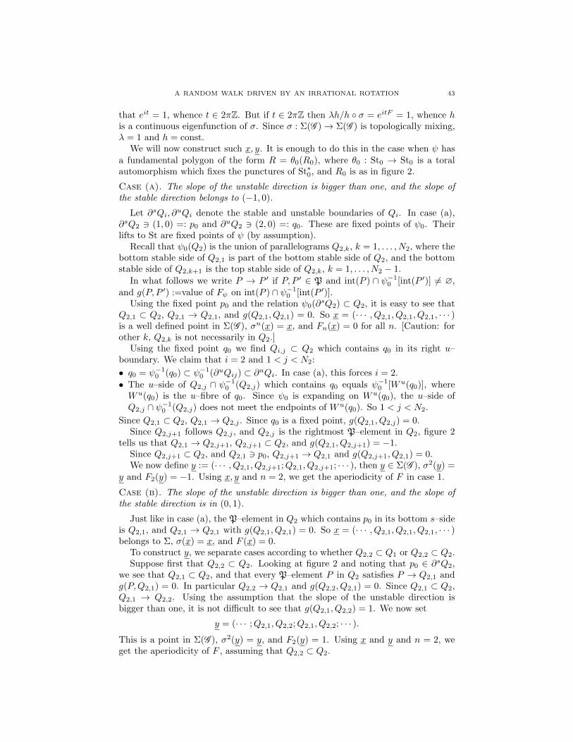
A RANDOM WALK DRIVEN BY AN IRRATIONAL ROTATION 43
that eit = 1, whence t ∈ 2πZ. But if t ∈ 2πZ then λh/h σ = eitF = 1, whence his a continuous eigenfunction of σ. Since σ : Σ(G )→ Σ(G ) is topologically mixing,λ = 1 and h = const.
We will now construct such x, y. It is enough to do this in the case when ψ hasa fundamental polygon of the form R = θ0(R0), where θ0 : St0 → St0 is a toralautomorphism which fixes the punctures of St∗0, and R0 is as in figure 2.
Case (a). The slope of the unstable direction is bigger than one, and the slope ofthe stable direction belongs to (−1, 0).
Let ∂sQi, ∂uQi denote the stable and unstable boundaries of Qi. In case (a),
∂sQ2 3 (1, 0) =: p0 and ∂uQ2 3 (2, 0) =: q0. These are fixed points of ψ0. Theirlifts to St are fixed points of ψ (by assumption).
Recall that ψ0(Q2) is the union of parallelograms Q2,k, k = 1, . . . , N2, where thebottom stable side of Q2,1 is part of the bottom stable side of Q2, and the bottomstable side of Q2,k+1 is the top stable side of Q2,k, k = 1, . . . , N2 − 1.
In what follows we write P → P ′ if P, P ′ ∈ P and int(P ) ∩ ψ−10 [int(P ′)] 6= ∅,
and g(P, P ′) :=value of Fψ on int(P ) ∩ ψ−10 [int(P ′)].
Using the fixed point p0 and the relation ψ0(∂sQ2) ⊂ Q2, it is easy to see thatQ2,1 ⊂ Q2, Q2,1 → Q2,1, and g(Q2,1, Q2,1) = 0. So x = (· · · , Q2,1, Q2,1, Q2,1, · · · )is a well defined point in Σ(G ), σn(x) = x, and Fn(x) = 0 for all n. [Caution: forother k, Q2,k is not necessarily in Q2.]
Using the fixed point q0 we find Qi,j ⊂ Q2 which contains q0 in its right u–boundary. We claim that i = 2 and 1 < j < N2:
• q0 = ψ−10 (q0) ⊂ ψ−1
0 (∂uQij) ⊂ ∂uQi. In case (a), this forces i = 2.
• The u–side of Q2,j ∩ ψ−10 (Q2,j) which contains q0 equals ψ−1
0 [Wu(q0)], whereWu(q0) is the u–fibre of q0. Since ψ0 is expanding on Wu(q0), the u–side ofQ2,j ∩ ψ−1
0 (Q2,j) does not meet the endpoints of Wu(q0). So 1 < j < N2.
Since Q2,1 ⊂ Q2, Q2,1 → Q2,j . Since q0 is a fixed point, g(Q2,1, Q2,j) = 0.Since Q2,j+1 follows Q2,j , and Q2,j is the rightmost P–element in Q2, figure 2
tells us that Q2,1 → Q2,j+1, Q2,j+1 ⊂ Q2, and g(Q2,1, Q2,j+1) = −1.Since Q2,j+1 ⊂ Q2, and Q2,1 3 p0, Q2,j+1 → Q2,1 and g(Q2,j+1, Q2,1) = 0.We now define y := (· · · , Q2,1, Q2,j+1;Q2,1, Q2,j+1; · · · ), then y ∈ Σ(G ), σ2(y) =
y and F2(y) = −1. Using x, y and n = 2, we get the aperiodicity of F in case 1.
Case (b). The slope of the unstable direction is bigger than one, and the slope ofthe stable direction is in (0, 1).
Just like in case (a), the P–element in Q2 which contains p0 in its bottom s–sideis Q2,1, and Q2,1 → Q2,1 with g(Q2,1, Q2,1) = 0. So x = (· · · , Q2,1, Q2,1, Q2,1, · · · )belongs to Σ, σ(x) = x, and F (x) = 0.
To construct y, we separate cases according to whether Q2,2 ⊂ Q1 or Q2,2 ⊂ Q2.Suppose first that Q2,2 ⊂ Q2. Looking at figure 2 and noting that p0 ∈ ∂sQ2,
we see that Q2,1 ⊂ Q2, and that every P–element P in Q2 satisfies P → Q2,1 andg(P,Q2,1) = 0. In particular Q2,2 → Q2,1 and g(Q2,2, Q2,1) = 0. Since Q2,1 ⊂ Q2,Q2,1 → Q2,2. Using the assumption that the slope of the unstable direction isbigger than one, it is not difficult to see that g(Q2,1, Q2,2) = 1. We now set
y = (· · · ;Q2,1, Q2,2;Q2,1, Q2,2; · · · ).
This is a point in Σ(G ), σ2(y) = y, and F2(y) = 1. Using x and y and n = 2, weget the aperiodicity of F , assuming that Q2,2 ⊂ Q2.
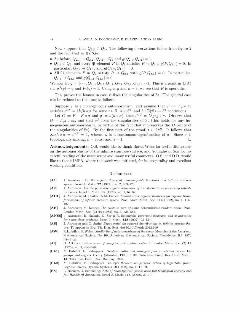
44 A. AVILA, D. DOLGOPYAT, E. DURYEV, AND O. SARIG
Now suppose that Q2,2 ⊂ Q1. The following observations follow from figure 2and the fact that p0 ∈ ∂sQ2:
• As before, Q2,1 → Q2,2, Q2,2 ⊂ Q1 and g(Q2,1, Q2,2) = 1.• Q1,1 ⊂ Q2, and every P–element P in Q1 satisfies P → Q1,1, g(P,Q1,1) = 0. In
particular, Q2,2 → Q1,1, and g(Q2,2, Q1,1) = 0.• All P–elements P in Q2 satisfy P → Q2,1 with g(P,Q2,1) = 0. In particular,Q1,1 → Q2,1 and g(Q1,1, Q2,1) = 0.
We now let y := (· · · ;Q2,1, Q2,2, Q1,1;Q2,1, Q2,2, Q1,1; · · · ). This is a point in Σ(G )
s.t. σ3(y) = y and F3(y) = 1. Using x, y and n = 3, we see that F is aperiodic.
This proves the lemma in case ψ fixes the singularities of St. The general casecan be reduced to this case as follows.
Suppose ψ is a homogeneous automorphism, and assume that F := Fψ π0
satisfies eitF = λh/h σ for some t ∈ R, λ ∈ S1, and h : Σ(G )→ S1 continuous.Let G := F + F σ and g := h(h σ), then eitG = λ2g/g σ. Observe that
G = Fψ2 π0, and that ψ2 fixes the singularities of St (this holds for any ho-mogeneous automorphism, by virtue of the fact that it preserves the D–orbits ofthe singularities of St). By the first part of the proof, t ∈ 2πZ. It follows thatλh/h σ = eitF = 1, whence h is a continuous eigenfunction of σ. Since σ istopologically mixing, h = const and λ = 1.
Acknowledgements. O.S. would like to thank Barak Weiss for useful discussionson the automorphisms of the infinite staircase surface, and Younghwan Son for hiscareful reading of the manuscript and many useful comments. O.S. and D.D. wouldlike to thank IMPA, where this work was initiated, for its hospitality and excellentworking conditions.
References
[A1] J. Aaronson: On the ergodic theory of non-integrable functions and infinite measurespaces. Israel J. Math. 27 (1977), no. 2, 163–173.
[A2] J. Aaronson: On the pointwise ergodic behaviour of transformations preserving infinite
measures. Israel J. Math. 32 (1979), no. 1, 67–82.[ADF] J. Aaronson; M. Denker; A.M. Fisher: Second order ergodic theorems for ergodic trans-
formations of infinite measure spaces. Proc. Amer. Math. Soc. 114 (1992), no. 1, 115–
127.[AK] J. Aaronson; M. Keane: The visits to zero of some deterministic random walks. Proc.
London Math. Soc. (3) 44 (1982), no. 3, 535–553.[ANSS] J. Aaronson; H. Nakada; O. Sarig; R. Solomyak: Invariant measures and asymptotics
for some skew products. Israel J. Math. 128 (2002), 93–134.
[AS] J. Aaronson and O. Sarig: Exponential chi squared distributions in infinite ergodic the-ory. To appear in Erg. Th. Dyn. Syst. doi:10.1017/etds.2012.160
[AW] R.L. Adler; B. Weiss: Similarity of automorphisms of the torus. Memoirs of the American
Mathematical Society, No. 98, American Mathematical Society, Providence, R.I. 1970ii+43 pp.
[At] G. Atkinson: Recurrence of co-cycles and random walks. J. London Math. Soc. (2) 13
(1976), no. 3, 486–488.[BL1] M. Babillot; F. Ledrappier: Geodesic paths and horocycle flow on abelian covers. Lie
groups and ergodic theory (Mumbai, 1996), 1–32, Tata Inst. Fund. Res. Stud. Math.,
14, Tata Inst. Fund. Res., Bombay, 1998.[BL2] M. Babillot; F. Ledrappier: Lalley’s theorem on periodic orbits of hyperbolic flows.
Ergodic Theory Dynam. Systems 18 (1998), no. 1, 17–39.
[BS] L. Barreira; J. Schmeling: Sets of “non-typical” points have full topological entropy andfull Hausdorff dimension. Israel J. Math. 116 (2000), 29–70.
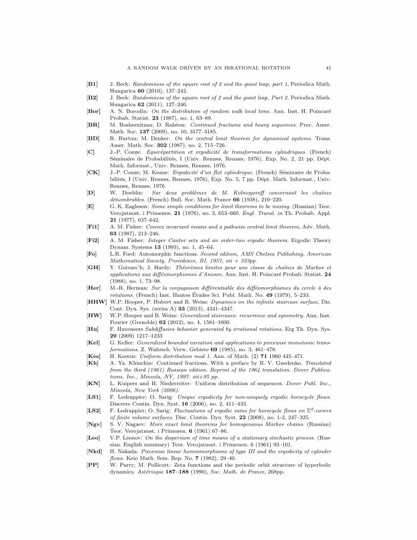
A RANDOM WALK DRIVEN BY AN IRRATIONAL ROTATION 45
[B1] J. Beck: Randomness of the square root of 2 and the giant leap, part 1, Periodica Math.
Hungarica 60 (2010), 137–242.
[B2] J. Beck: Randomness of the square root of 2 and the giant leap, Part 2. Periodica Math.Hungarica 62 (2011), 127–246.
[Bor] A. N. Borodin: On the distribution of random walk local time. Ann. Inst. H. Poincare
Probab. Statist. 23 (1987), no. 1, 63–89.[BR] M. Boshernitzan; D. Ralston: Continued fractions and heavy sequences. Proc. Amer.
Math. Soc. 137 (2009), no. 10, 3177–3185.
[BD] R. Burton; M. Denker: On the central limit theorem for dynamical systems. Trans.Amer. Math. Soc. 302 (1987), no. 2, 715–726.
[C] J.-P. Conze: Equirepartition et ergodicite de transformations cylindriques. (French)
Seminaire de Probabilites, I (Univ. Rennes, Rennes, 1976), Exp. No. 2, 21 pp. Dept.Math. Informat., Univ. Rennes, Rennes, 1976.
[CK] J.-P. Conze; M. Keane: Ergodicite d’un flot cylindrique. (French) Seminaire de Proba-bilites, I (Univ. Rennes, Rennes, 1976), Exp. No. 5, 7 pp. Dept. Math. Informat., Univ.
Rennes, Rennes, 1976.
[D] W. Doeblin: Sur deux problemes de M. Kolmogoroff concernant les chaınesdenombrables. (French) Bull. Soc. Math. France 66 (1938), 210–220.
[E] G. K. Eagleson: Some simple conditions for limit theorems to be mixing. (Russian) Teor.
Verojatnost. i Primenen. 21 (1976), no. 3, 653–660. Engl. Transl. in Th. Probab. Appl.21 (1977), 637–642.
[Fi1] A. M. Fisher: Convex invariant means and a pathwise central limit theorem, Adv. Math.
63 (1987), 213–246.[Fi2] A. M. Fisher: Integer Cantor sets and an order-two ergodic theorem. Ergodic Theory
Dynam. Systems 13 (1993), no. 1, 45–64.
[Fo] L.R. Ford: Automorphic functions. Second edition, AMS Chelsea Publishing, AmericanMathematical Society, Providence, RI, 1957, xii + 333pp.
[GH] Y. Guivarc’h; J. Hardy: Theoremes limites pour une classe de chaınes de Markov etapplications aux diffeomorphismes d’Anosov. Ann. Inst. H. Poincare Probab. Statist. 24
(1988), no. 1, 73–98.
[Her] M.-R. Herman: Sur la conjugaison differentiable des diffeomorphismes du cercle a des
rotations. (French) Inst. Hautes Etudes Sci. Publ. Math. No. 49 (1979), 5–233.
[HHW] W.P. Hooper, P. Hubert and B. Weiss: Dynamics on the infinite staircase surface, Dis.Cont. Dyn. Sys. (series A) 33 (2013), 4341–4347.
[HW] W.P. Hooper and B. Weiss: Generalized staircases: recurrence and symmetry. Ann. Inst.
Fourier (Grenoble) 62 (2012), no. 4, 1581–1600.[Hu] F. Huveneers Subdiffusive behavior generated by irrational rotations, Erg Th. Dyn. Sys.
29 (2009) 1217–1233
[Kel] G. Keller: Generalized bounded variation and applications to piecewise monotonic trans-formations, Z. Wahrsch. Verw. Gebiete 69 (1985), no. 3, 461–478.
[Kes] H. Kesten: Uniform distribution mod 1. Ann. of Math. (2) 71 1960 445–471.[Kh] A. Ya. Khinchin: Continued fractions. With a preface by B. V. Gnedenko. Translated
from the third (1961) Russian edition. Reprint of the 1964 translation. Dover Publica-tions, Inc., Mineola, NY, 1997. xii+95 pp.
[KN] L. Kuipers and H. Niederreiter: Uniform distribution of sequences. Dover Publ. Inc.,
Mineola, New York (2006).
[LS1] F. Ledrappier; O. Sarig: Unique ergodicity for non-uniquely ergodic horocycle flows.Discrete Contin. Dyn. Syst. 16 (2006), no. 2, 411–433.
[LS2] F. Ledrappier; O. Sarig: Fluctuations of ergodic sums for horocycle flows on Zd-coversof finite volume surfaces. Disc. Contin. Dyn. Syst. 22 (2008), no. 1-2, 247–325.
[Ngv] S. V. Nagaev: More exact limit theorems for homogeneous Markov chains. (Russian)
Teor. Verojatnost. i Primenen. 6 (1961) 67–86.
[Leo] V.P. Leonov: On the dispersion of time means of a stationary stochastic process. (Rus-sian. English summary) Teor. Verojatnost. i Primenen. 6 (1961) 93–101.
[Nkd] H. Nakada: Piecewise linear homeomorphisms of type III and the ergodicity of cylinderflows. Keio Math. Sem. Rep. No. 7 (1982), 29–40.
[PP] W. Parry; M. Pollicott: Zeta functions and the periodic orbit structure of hyperbolic
dynamics. Asterisque 187–188 (1990), Soc. Math. de France, 268pp.
46 A. AVILA, D. DOLGOPYAT, E. DURYEV, AND O. SARIG
[Pe] Y. Peres: A combinatorial application of the maximal ergodic theorem, Bull. London
Math. Soc. 20 (1988), 248–252.
[Pet] K. Petersen: Ergodic theory. Cambridge Studies in Advanced Mathematics, 2. Cam-bridge University Press, Cambridge, 1983. xii+329 pp. ISBN: 0-521-23632-0
[PS] W. Philipp; W. Stout: Almost sure invariance principles for partial sums of weakly
dependent random variables. Mem. Amer. Math. Soc. 2 161 iv+140pp.[Ra] D. Ralston: 1
2-Heavy Sequences Driven By Rotation. Preprint arXiv:1106.0577.
[RS] L. Rocadas; J. Schoißengeier: On the local discrepancy of (nα)-sequences. J. NumberTheory 131 (2011), no. 8, 1492–1497.
[Ru] D. Ruelle: Thermodynamic formalism. The mathematical structures of classical equi-
librium statistical mechanics. With a foreword by Giovanni Gallavotti and Gian-CarloRota. Encyclopedia of Mathematics and its Applications, 5 Addison-Wesley Publishing
Co., Reading, Mass., 1978. xix+183 pp.
[Sa] O.M. Sarig: Unique ergodicity for infinite measures. Proceedings of the InternationalCongress of Mathematicians. Volume III, 1777–1803, Hindustan Book Agency, New
Delhi, 2010.
[SS] O. Sarig; B. Schapira: The generic points for the horocycle flow on a class of hyperbolicsurfaces with infinite genus. Int. Math. Res. Not. 2008, Art. ID rnn 086, 37 pp.
[Sch] K. Schmidt: A cylinder flow arising from irregularity of distribution. Compositio Math.36 (1978), no. 3, 225–232.
[V] D. Volny: Invariance principles and Gaussian approximation for strictly stationary pro-
cesses. Trans. Amer. Math. Soc. 351 (1999), no. 8, 3351–3371.
A. Avila, CNRS U.M.R. 7586 Institut de Mathematiques de Jussieu - Paris Rive Gauche,Batiment Sophie Germain, Case 7012, 75205 Paris Cedex 13, France and IMPA Estrada
Dona Castorina, 110 Rio de Janeiro, 22460-320 Brasil
E-mail address: [email protected]
D. Dolgopyat, 4417 Mathematics Bldg, University of Maryland, College Park, MD
20742, USAE-mail address: [email protected]
E. Duryev, Department of Mathematics, Faculty of Arts and Sciences, Harvard Uni-versity, 1 Oxford Street Cambridge MA 02138 USA
E-mail address: [email protected]
O. Sarig, Faculty of Mathematics and Computer Science, Weizmann Institute ofScience, 234 Herzl Street, Rehovot, 7610001 Israel
E-mail address: [email protected]


![Random walk on mated-CRT planar maps and Liouville ... › pdf › 2003.10320.pdfspectral dimension, and a paper by Gwynne and Hutchcroft [GH18] which proves the upper bound for the](https://static.fdocument.org/doc/165x107/5f1c12d3b9ca474d454633df/random-walk-on-mated-crt-planar-maps-and-liouville-a-pdf-a-200310320pdf.jpg)