The structure of zonal jets in geostrophic turbulencerks/preprints/scott_dritschel_jfm_2012.pdf ·...

Under consideration for publication in J. Fluid Mech. 1

The structure of zonal jets in geostrophicturbulence

By RICHARD K. SCOTT AND DAVID G. DRITSCHELSchool of Mathematics and Statistics

University of St Andrews, St Andrews KY16 9SS, Scotland

(Received 24 August 2012)

The structure of zonal jets arising in forced-dissipative, two-dimensional turbulent flowon the β-plane is investigated using high-resolution, long-time numerical integrations,with particular emphasis on the late-time distribution of potential vorticity. The structureof the jets is found to depend in a simple way on a single non-dimensional parameter,which may be conveniently expressed as the ratio LRh/Lε, where LRh =

√U/β and

Lε = (ε/β3)1/5 are two natural length scales arising in the problem; here U may be takenas the root-mean-square velocity, β is the background gradient of potential vorticity inthe north-south direction, and ε is the rate of energy input by the forcing. It is shownthat jet strength increases with LRh/Lε, with the limiting case of the potential vorticitystaircase, comprising a monotonic, piecewise-constant profile in the north-south direction,being approached for LRh/Lε ∼ O(10). At lower values, eddies created by the forcingbecome sufficiently intense to continually disrupt the steepening of potential vorticitygradients in the jet cores, preventing strong jets from developing. Although detailedfeatures such as the regularity of jet spacing and intensity are found to depend on thespectral distribution of the forcing, the approach of the staircase limit with increasingLRh/Lε is robust across a variety of different forcing types considered.

1. IntroductionLarge-scale zonal (longitudinally aligned) jets are observed in a wide range of geophys-

ical flows including those of the terrestrial atmosphere and oceans and the atmospheresof the gas giant planets. They coexist with a background of inhomogeneous turbulentmotions and the relative intensity of the jets to the turbulent background has a stronginfluence on the meridional transport of important quantities such as heat, momentum,and constituent tracers, the latter including chemically and thermodynamically impor-tant quantities such as ozone and water vapour. The interplay between the jets and theturbulent background is highly complex, turbulent motions being organized into latitudi-nal bands by the jets, the jets themselves being maintained against dissipation via eddymomentum fluxes (see, e.g., the recent review by McIntyre 2008, and references therein).

The fact that jets are observed in such a wide range of dynamical regimes, and in thepresence of very different forcing mechanisms, suggests that robust dynamical processesare involved in their generation. It has been argued, for example, that the strong jetsobserved in the Jovian atmosphere are dynamically similar to the much weaker jetsobserved in the oceans (Galperin et al. 2004). However, beyond the conclusion that thejets are driven by eddy momentum fluxes in each case, the similarities and differencesare not well understood. In particular, it is unclear what controls fundamental propertiessuch as the intensity, spacing, and steadiness of the jets in these cases.

2 R. K. Scott & D. G. Dritschel

Regarding the spacing of the jets, it has long been understood that it is closely linkedto a fundamental length scale of the flow, the Rhines scale, given by LRh =

√U/β

(Rhines 1975; Williams 1978), where U is a typical velocity scale of the flow and β is thelocal background latitudinal gradient of potential vorticity (comprising, in the simplestcontext, the relative vorticity and the vorticity due to the planetary rotation). The Rhinesscale LRh may be considered as the scale at which zonal motions become important, or,equivalently, the scale at which a background of quasi-two dimensional turbulent motionbegins to project significantly onto the lower frequencies of freely propagating Rossbywaves (see, e.g., Vallis 2006, for an overview). However, the precise relation between LRh

and jet spacing is complicated both by the ambiguity in the choice of U , for example,whether it represents an eddy or jet velocity, and by the effect of strong mean flows onthe linear Rossby wave propagation. In an evolving flow, it is therefore difficult to predicta priori the spacing of jets that will emerge.

Although forcing mechanisms may vary enormously in different situations, the forma-tion and final structure of jets may be described quite generally in terms of the quasi-horizontal mixing of the background gradient of potential vorticity by eddies. Due tothe constraints of strong stable stratification and rapid rotation, the large-scale motionsof planetary atmospheres and oceans may, to a first approximation, be characterized bytheir quasi-two dimensional motion. Zonal jets arise inevitably when potential vorticityis mixed horizontally over limited latitudinal regions, regardless of the form of the mixing(McIntyre 1982; Dritschel & McIntyre 2008; Dunkerton & Scott 2008; McIntyre 2008;Scott 2010). Potential vorticity mixing by planetary scale Rossby waves in the polar win-ter stratosphere was discussed already by McIntyre (1982), who noted the tendency formixing to weaken potential vorticity gradients in a “surf zone”, while intensifying themon either side, resulting in an intensification of the polar night jet. An analogous effectin the case of vertical mixing by internal waves in a stratified fluid was discussed stillearlier by Phillips (1972). In the case of the polar night jet, a large scale flow is forcedby radiative processes, which is eddy intensified into a stronger, sharper jet. However,the material conservation of potential vorticity suggests that any nonlinear eddy motionswill suffice to mix the background gradient, which may be considered as “an unstableequilibrium in the presence of Rossby waves and instabilities” (Dunkerton & Scott 2008).Thus, while eddies may arise from a variety of sources such as local instability or Rossbywave propagation, their effect on the jet formation may be considered universal in thatit involves the mixing of the background potential vorticity. In the cases of the Jovianand oceanic jets, the forcing serves to mix the potential vorticity, but the precise detailsare of secondary importance.

The so-called potential vorticity staircase describes the limiting case in which the back-ground potential vorticity is mixed perfectly in distinct latitudinal regions, separated bystrong gradients at the jet cores. It has been put forward as a model for the Jovian jets(Marcus 1993; Peltier & Stuhne 2002). In this model, sharp jets correspond to the strongpotential vorticity gradients separating mixed zones. It was investigated more recently byDunkerton & Scott (2008) and Dritschel & McIntyre (2008), who derived simple expres-sions for the relation between jet spacing and jet strength, reviewed in section 2 below. Inthis paper, a second question is addressed, namely, under what conditions, if any, can thestaircase limit be achieved in an evolving forced turbulent flow. Or, more generally, whatcontrols the extent of mixing by the turbulent flow. By a series of numerical experiments,described in section 4 below, we demonstrate that the extent of mixing is controlled by asingle non-dimensional parameter that may be conveniently expressed as a ratio of twolength scales: the Rhines scale LRh; and a length scale, introduced originally by Maltrud& Vallis (1991), that describes the intensity of the forcing relative to the background

The structure of zonal jets 3

potential vorticity gradient Lε = (ε/β3)1/5, where ε is the rate of energy input by theforcing. Essentially, the strength of zonal jets and the steepness of potential vorticitygradients in the jet cores increase as the ratio LRh/Lε is increased. The staircase limit isapproached for LRh/Lε ∼ O(10). For LRh/Lε ∼ O(1), below a value of around 5, on theother hand, the jets and the potential vorticity gradients in the jet cores remain stronglyperturbed by the eddy activity of the background turbulent flow.

The dependence of jet strength on a parameter similar to LRh/Lε has been dis-cussed previously (Vallis 2006; Sukoriansky et al. 2007), but largely on phenomenologicalgrounds, and in relation to the halting of the inverse cascade through frictional effects.In the two-dimensional barotropic equations under consideration, with specified β, to-tal energy, and energy input rate, it is the single non-dimensional parameter controllingthe system state. However, the relation between this parameter and the organizationof potential vorticity into a staircase-like distribution has not previously been consid-ered. Part of the reason for this is that previous numerical experiments have typicallynot observed flows with strong staircase-like distributions (e.g. Sukoriansky et al. 2007),leading some to question the realizability of such distributions in any physical system.As demonstrated here, the staircase limit is indeed realizable, but only under conditionsof exceptionally weak forcing, for which the staircase emerges on correspondingly longtime scales. The extremely long integration times required, together with the need forhigh resolution, may partly explain why such strong staircase-like distributions have notbeen observed and why the simple relation to LRh/Lε has not been documented.

Of course, the structure of jets might also depend not just on the total energy and theenergy input rate of the forcing, but also on details of the physical mechanism throughwhich the forcing increases the energy of the system. In reality, a quasi-two dimen-sional atmospheric flow may be forced via a variety of physical mechanisms, includingshear instability, both barotropic and baroclinic, convective penetration from an under-lying layer, or flow over topography. The common practice in numerical investigations oftwo-dimensional turbulence is to ignore such distinctions and use a simple band-limitedspectral-space forcing as the crudest representation of all these physical processes, thetacit assumption being that the energy input rate is the most important factor controllingthe turbulent evolution. Band-limited spectral-space forcing may be the most relevantrepresentation of forcing via shear instability in baroclinic models, where the dominantunstable mode is located at a distinct wavenumber (which in a fully three-dimensionalmodel would be controlled to an extent by the internal deformation radius). To exam-ine the degree to which the forcing mechanism does influence the final jet structure, weconsider three qualitatively distinct types of forcing. In addition to the usual forcing ofthe band-limited spectral-space type, we also consider two types of forcing with a broadwavenumber spectrum, which may be more relevant to the physical process of convectivepenetration. The three different forcing types and their implementation are discussedfurther in section 3.3 below. Although the form of the forcing affects some details ofthe resulting jet structure, we emphasize that our main result, that the staircase limit isapproached for LRh/Lε ∼ O(10), is found in all cases.

2. Jet spacing in the staircase limitThe natural tendency of eddy motions to mix background potential vorticity explains

the ubiquity of zonal jets in atmospheres and oceans and their existence in such a varietyof physical situations. The evolution of the potential vorticity field towards a staircase-like distribution may be understood intuitively as a result of the tendency of strongpotential vorticity gradients to suppress further (latitudinal) mixing, an effect described


as Rossby wave elasticity: a perturbation made to a region of strong gradients will beradiated as Rossby waves, rather than result in an irreversible deformation of the gra-dients themselves. Conversely, regions of weak potential vorticity gradients are highlysusceptible to deformation and further mixing. The combined result is a positive feed-back whereby mixing is enhanced in regions of weak gradients and suppressed in regionsof strong gradients. When waves or eddies are present in the flow, any local reduction orintensification of potential vorticity gradients will be enhanced. If the mixing/steepeningprocesses are allowed to continue unabated (the conditions for this will be discussed insection 4 below) then the potential vorticity structure will evolve into a staircase-likestructure, comprising a monotonic piecewise constant distribution in latitude (regionsof zero potential vorticity gradient separated by isolated discontinuities or jumps in lat-itude). See recent reviews by Baldwin et al. (2007); McIntyre (2008); Scott (2010) forfurther discussion.

The jumps of potential vorticity in latitude correspond, through the diagnostic relationbetween potential vorticity and velocity, to sharply peaked, zonally aligned, eastward jets(see e.g. Dritschel & McIntyre 2008, figure 7). It is worth noting that the above descriptionexplains quite naturally the asymmetry between eastward and westward jets sometimesdiscussed in the literature. In this description, only the eastward jets are true jets, thewestward flow being merely a return flow required by mass conservation. Put anotherway, the regions of steep potential vorticity gradients naturally define the jet cores. Thedistinction is important when considering jets as potential barriers to the latitudinaltransport of chemical species.

The limit of a zonally symmetric perfect potential vorticity staircase, comprised ofmonotonic piecewise constant potential vorticity in the latitudinal direction, allows asimple analytic relation to be obtained relating the spacing between the jumps to thestrength of the associated jets. Two separate cases were considered recently: the case ofsingle layer quasi-geostrophic barotropic flow on the sphere (Dunkerton & Scott 2008);and the case of single layer quasi-geostrophic equivalent barotropic flow on the β-plane(Dritschel & McIntyre 2008). In both cases the half-separation of the jets, Lj , or thedistance between adjacent peak eastward and westward velocity, is given by

Lj =√

3LRh

where LRh is defined with U denoting the peak eastward velocity † . In the equivalentbarotropic case studied by Dritschel & McIntyre (2008), the result is exact in the limitof infinite Rossby deformation length, LD (defined in the parent shallow water system asthe ratio of gravity wave speed to rotation). In the barotropic case studied by Dunkerton& Scott (2008), the result is asymptotic in latitude, being exact for a staircase profilelocalized near the equator, but holding to a good approximation in midlatitudes. Theresult is essentially dependent only on the background angular momentum profile havinga quadratic dependence in the latitudinal coordinate (sine of latitude on the sphere).

The result can be extended qualitatively to the case of a smoother potential vorticitydistribution (retaining the assumption of zonal symmetry). If, starting from a staircase ofa given jet separation, we smooth the jumps in potential vorticity at the jets, we reducethe maximum jet speed while retaining the same jet separation. Conversely, a smoothstaircase with the same jet speed would have jets that were spaced farther apart thanthose of the limiting case described above. The relation between jet spacing and jet speed

† Note that the prefactors of√

2 and√

6 used in Dritschel & McIntyre (2008) and Dunkerton& Scott (2008), respectively, result from slight variations in the definition of LRh.


may therefore be considered as an inequality

Lj ≥√

3LRh,

which holds for all zonally symmetric profiles, and with equality for the piecewise constantstaircase described above.

In the numerical experiments described below it is convenient to define LRh not usingthe maximum jet speed U , but rather using the root-mean-square velocity Urms, relatedto the total energy of the flow. In doing so, the relation between jet spacing and strengthis modified slightly to Lj ≥ 451/4LRh, the prefactor here being increased by a factor of51/4. (This inequality is valid provided, of course, that Urms is taken as the root-mean-square of u(y), that is, neglecting the energy in the eddy field. In fact, for well-developedjet flows in the barotropic case studied here, nearly all the energy is indeed contained inthe zonal mean flow, significant eddy kinetic energy being found only in cases very farfrom the staircase limit, as demonstrated below.)

Although the perfect staircase limit is convenient analytically and provides a boundon the jet spacing of a flow of given energy, the question remains of when, if at all,such complete potential vorticity homogenization may occur in a turbulent flow. Someauthors have suggested that only weak potential vorticity mixing takes place resultingin potential vorticity distributions that are far from the staircase limit. On the otherhand, staircase-like potential vorticity distributions have certainly been obtained, evenat relatively modest numerical resolution (e.g. Scott & Polvani 2007, figure 10 therein). Inthat paper, attention was already drawn to the effect of forcing strength on the potentialvorticity structure. Figures 2 and 3 of Scott & Polvani (2007) compared two cases withidentical final energy E = ε/2r in a forced case with frictional damping at rate r, butwith values of ε and r that differed by a factor of ten. In the weakest forcing case thejet structure was markedly more pronounced. The numerical experiments described nextwill examine this question in more detail, varying the forcing and damping over a widerrange to explore more carefully the approach to the staircase limit.

3. The physical model3.1. Equations of motion

We consider the quasi-geostrophic approximation to the rotating shallow water equationson the β-plane, where the Coriolis parameter f = f0 + βy is linear in y with constantgradient β. We allow for the input of energy via a prescribed forcing and the dissipationof energy by linear friction at rate r. The equations reduce to the material advection ofquasi-geostrophic potential vorticity, q, with the forcing and dissipation represented assource terms F and −rζ, breaking exact material conservation:

qt + J(ψ, q) = F − rζ, (3.1)

where J is the Jacobean determinant and ζ = ∇2ψ is the relative vorticity. The advectingflow is determined by the streamfunction ψ which is related to q through

q = βy +∇2ψ − L−2D ψ, (3.2)

where LD =√gH/f0 is the Rossby deformation length and where g is gravity and H

is the mean layer depth. Throughout this paper we consider the limit L−1D → 0 only,

corresponding to the case of purely two-dimensional, barotropic vortex dynamics. Thecase of nonzero L−1

D , arguably more relevant to the case in which energy is input viabaroclinic instability of a background vertical shear (e.g. Panetta 1993), will be treatedin a companion paper.


3.2. Numerical implementationEquation (3.1) is integrated numerically in a doubly-periodic domain of length 2π in boththe x and y directions. The integration is carried out using an extension of the contour-advective semi-Lagrangian algorithm developed by Dritschel & Ambaum (1997) thatboth enables the implementation of arbitrary forcing functions F , and more accuratelyevolves the energy at large scales. Full details and numerical tests of the extension may befound in Fontane & Dritschel (2009); Dritschel & Fontane (2010); here, for completeness,we summarise the main points.

The new algorithm makes use of a three-way decomposition of the potential vortic-ity field into (i) a component qs integrated using a pseudo-spectral method for accuraterepresentation of the large-scale flow; (ii) a component qa integrated using a contour-advective method for accurate representation of the intermediate to small-scale flow; and(iii) a component qd used to represent the non-conservative forcing, and to compensatefor any errors involved in the contour representation of a smooth field. The latter maybe integrated using either a vortex-in-cell method or a pseudo-spectral method as ap-propriate for the particular choice of forcing (see section 3.3 below). The three fields arecombined at each timestep using a spectral low-pass filter applied to qs and its com-plement applied to qa, retaining the large-scale parts of qs and the intermediate andsmall-scale parts of qa; the combination of solutions ensures that each method is usedwhere it is most accurate.

At regular intervals, based on the maximum vorticity of the flow (in practice aboutevery 160 time steps), the contoured field qa is regenerated from the full potential vorticityfield, obtained simply by summing the three fields qa, qs, and qd on a fine grid. Thisfine grid, which in the calculations reported here comprises 2048 × 2048 grid pointsover the 2π × 2π domain, thus represents the effective resolution of the integration.Dissipation arising from contour surgery (Dritschel 1989), re-gridding of contours, andgridding of point vortices (when these are used) is effectively confined to scales strictlysmaller than the fine grid scale. An important feature is that the contour surgery itself hasalmost no effect on steep gradients of potential vorticity. The result is an exceptionallyweak dissipation compared to other standard methods, as a comparison for the case ofisotropic, freely-decaying, two-dimensional turbulence recently demonstrated (Dritschel& Scott 2009). In the integrations reported below, energy dissipation rates due to contoursurgery, re-contouring, and gridding are of the order of 10−4 times smaller than typicaldissipation rates due to friction, even in the most weakly damped cases.

The contoured field qa is advected using a velocity field obtained from the inversion ofthe combined qa, qs, and qd fields interpolated onto a coarse grid comprising 128 × 128grid points. The contour interval used to represent qa is chosen to give 200 contour levelsacross the domain at t = 0, i.e. to represent q in the range [−βπ, βπ]. This numberis sufficient to capture the weak variations of potential vorticity in nearly homogenizedregions of the flow at late times.

3.3. ForcingTo verify the robustness of our results we consider three qualitatively different types offorcing. The simplest, but arguably least realistic, comprises a narrow-band distributionin spectral space, centred around a specified wavenumber kf , and δ-correlated in time.It is popular in studies of the two-dimensional inverse energy cascade because it allows aclear inertial range in spectral space over which the effects of forcing are zero by construc-tion. The function F in (3.1) is defined in spectral space via its Fourier transform, fk,which satisfies 〈fkf∗k〉 = F (k)/πk with spectrum F (k) = ε for k = |k| ∈ [kf −δk, kf +δk]and F (k) = 0 otherwise, where ε is the rate of energy input, δk is a specified bandwidth,


and angle brackets denote an ensemble average. In the numerical implementation, thisforcing is added at each timestep to the field qd, which is periodically recombined withthe contour field, as described above.

The above case for which the forcing scale is precisely determined in spectral space maybe appropriate as a crude representation of a physical instability that has a well-defineddominant wavelength. This may be contrasted with a physical process such as convectivepenetration, which may be regarded (at the crudest approximation) as having a well-defined scale, lf , in physical space, and a correspondingly broad distribution in spectralspace. The second type of forcing used here is designed to represent such a physicalprocess in the case where lf is small. It is implemented numerically through the injectionof point vortices of a fixed circulation κv, in such a way that the enstrophy input, η, isconstant in time. Because, during the inversion stage, the vorticity of each point vortex isinterpolated onto the coarse grid, the length scale of the forcing may therefore be takenas lf = δx, the coarse grid length scale. The corresponding energy input rate is givenapproximately by η/k2

f , where kf = 2π/lf is the highest wavenumber resolved by thecoarse grid, which would be exact if all enstrophy were input at the wavenumber kf .

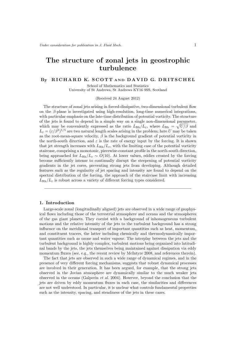
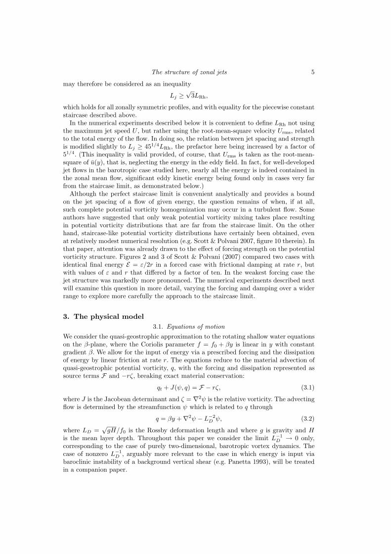
A variety of configurations for the input distribution of point vortices have been con-sidered: they may be input singly, as equal numbers of positive and negative monopoles,randomly distributed in space; as randomly oriented dipole pairs (with zero net circula-tion); or as quadrupoles (with zero net linear impulse). Likewise, the number of vorticesand their circulations must be chosen for a desired enstrophy input rate. All configura-tions of point vortices give qualitatively similar results, and for brevity we present belowonly those results obtained with dipole forcing. We note that in this case the orientationsof the dipoles are randomized to minimize the systematic input of linear momentum.In the case of quadrupole forcing, for which the linear momentum input is identicallyzero, each quadrupole tends to split immediately into a dipole pair and so the differencesbetween these two types of forcing are very small. For the dipole distribution, the forcingfunction F has energy and enstrophy spectra F (k) and k2F (k) whose forms are shown inFigure 1. Note that the enstrophy is input mainly at the highest resolved wavenumbers,whereas the energy has a much broader distribution in spectral space. †

The third type of forcing considered is a modified version of the physical-space forcingjust described. Energy is input in spectral space, with a forcing F that has the sameenergy spectrum F (k) as the one shown in Figure 1 but with randomized phases ofindividual Fourier modes. As in the case of narrow-band spectral-space forcing the fieldF is again added to the field qd.

When β = 0 all of the above types of forcing give a rate of energy input, ε0, intothe system that may be specified a priori. When β 6= 0 the situation is complicated bycorrelations between the forcing and the zonal mean flows that develop at late times.At early times, say for t � 1/r in the calculations presented below, before strong zonalmotions have developed and when the total energy of the flow is small enough thatfrictional dissipation can be neglected, the total energy E has been verified to growas expected like ε0t for all calculations considered, for some ε0 specified a priori. Atlater times, however, it was found that the actual energy input rates, ε, as derivedfrom the energy equation, E = ε − 2rE , where E is the measured total energy, tend toincrease beyond the value ε0. The effect is weak in most cases but is stronger in cases in

† The strength of the dipoles are chosen such that the associated maximum absolute vorticityon the grid is 2πα, for some constant α and from this is calculated the number of dipoles per unittime required to give the correct enstrophy input rate. The numerical constant α was set to 0.1;tests varying this value between 1 and 0.01 showed no significant effect on the flow evolution.

8 R. K. Scott & D. G. Dritschel0.025

032 64

k 2

10 3

k0

F

F

Figure 1: Energy and enstrophy spectra of the physical-space forcing using vortex dipoles.

which the zonal mean flow contains a greater proportion of the total energy, and is morepronounced when the forcing spectrum is broad, presumably because there is greaterscope for correlations between the mean flows and the forcing. The effect is strongestin cases of very weak forcing and damping, where the staircase limit is approached, andwhere the measured energy input rate may be as much as twenty times greater than ε0,depending on the type of forcing used.

Despite possibly significant differences between ε0 and ε, corresponding differences tothe key parameters in the system at equilibrium are small. In particular, taking LRh =√Urms/β = (2E)1/4β−1/2, and using ε = 2rE at equilibrium, the key non-dimensional

parameter LRh/Lε depends on ε as

LRh/Lε = β1/10r−1/4ε1/20, (3.3)

the 1/20th power giving a very weak dependence on the actual value of energy inputrate ε: a measured energy input rate ε exceeding the nominal value ε0 by a factor oftwenty, say, will only increase LRh/Lε by about 16%. To be definite in the analysis ofthe simulations presented below, however, the energy input rate into the system once astatistical equilibrium has been reached is always calculated a posteriori from the energyequation ε = 2rE .

3.4. Physical parametersEquation (3.1) is nondimensionalized such that the domain length L = 2π, and weconsider here only the case L−1

D = 0. A natural time scale may be defined in terms ofthe Rossby wave frequency for flows with a nominal characteristic length scale LRh0, asTβ = 2π/βLRh0. Here, LRh0 is defined as the Rhines scale (defined as LRh =

√Urms/β)

that would be obtained with a specified frictional rate r if the energy input rate ε wereto remain equal to the nominal value ε0 for the duration of the integration. Thus LRh0 =(ε0/r)1/4β−1/2, and here it is fixed to a value of LRh0 = 1/8, which was found to yielda reasonable number of jets across the domain in the integrations conducted. Settingβ = 16π then gives a convenient timescale of Tβ = 1, as well as an O(1) value ofU0 =

√ε0/r = π/4.


3 7 11LRh0 /L ε0

3

7

11

LRh /Lε

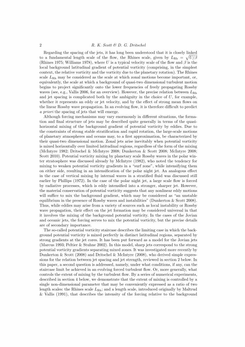
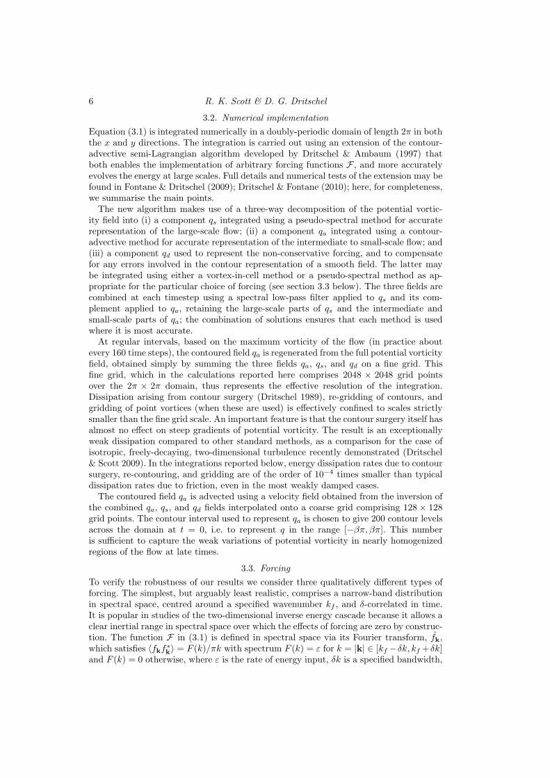
Figure 2: Actual LRh/Lε relative to nominal LRh0/Lε0, for r = 1×10−4 to r = 256×10−4

and all forcing types: physical-space forcing (triangles), narrow-band spectral space forc-ing (inverted triangles), broad-band spectral-space forcing (squares). Multiple symbolsfor single values of LRh0/Lε0 denote multiple realizations of the random forcing.

The choice LRh0 = 1/8 constrains the possible values of ε0 and r, through the relationε0/r = β2L4

Rh0. Keeping the ratio ε0/r fixed, ε0 and r are varied across a range of values toachieve LRh0/Lε0 approximately in the range [3, 10], where Lε0 = (ε0/β3)1/5. Specificallyr is varied from 0.0256, for which LRh0/Lε0 ≈ 3.0 to 0.0001 for which LRh0/Lε0 ≈ 9.11.As described in section 3.3, the actual values of ε, LRh, and Lε are always calculateda posteriori at equilibrium from the measured total energy via ε = 2rE , and typicallyexceed the nominal values. For completeness, in Figure 2 we show the dependence ofthe measured values of LRh/Lε against the nominal values for all simulations conducted:actual values exceed the nominal ones by up to about 18% for the weakest forcing casesand by a smaller amount at stronger forcing.

The energy of the flow equilibrates to the final value on a timescale of 1/r. To ensurethat the flow reaches a stationary state with respect to the formation of zonal jets, weintegrate (3.1) for a total time of 10/r. The stationarity of the flow by this time is verifiedin the numerical experiments below.

4. Realisability of the staircase4.1. Physical-space forcing

The results from the numerical experiments are presented next. We focus mainly on thecase of physical-space forcing by point vortex dipoles, as described in section 3.3 above.The results are compared with the case of spectral-space forcing in section 4.3.

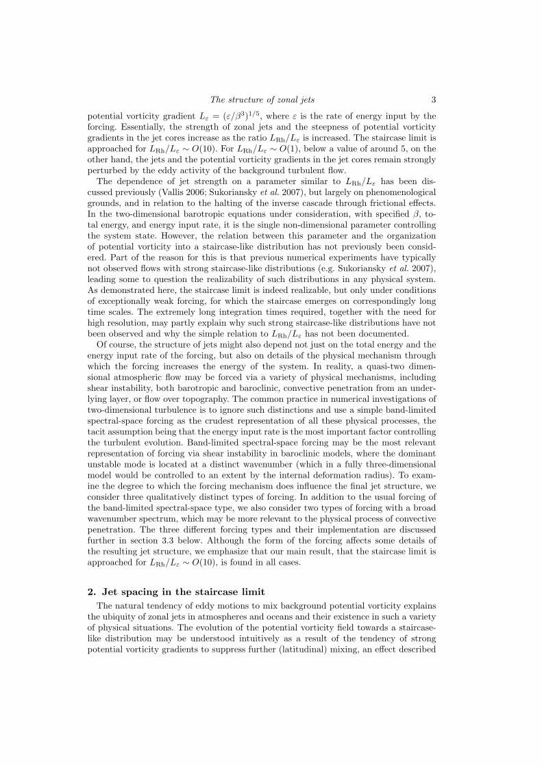
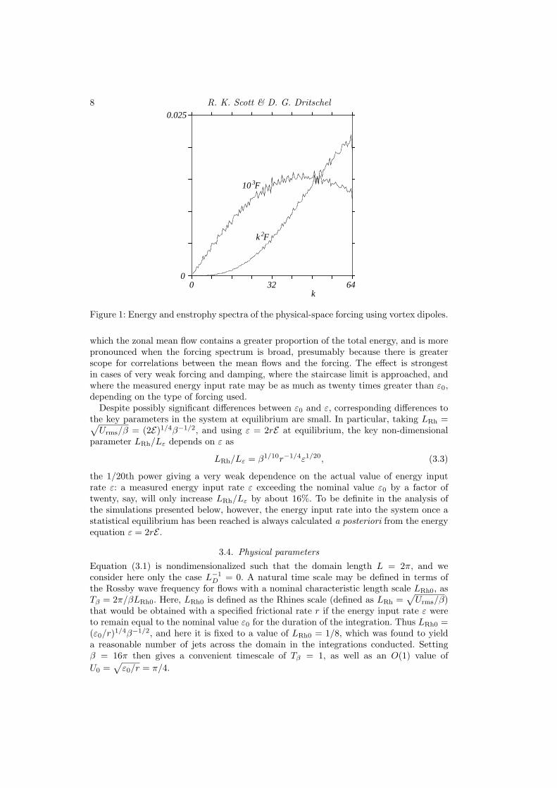
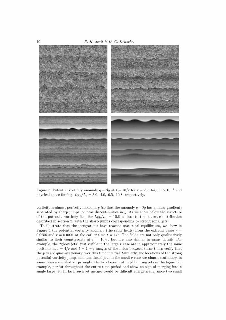
Figure 3 shows the potential vorticity anomaly q(x, y, t) − βy at the final integrationtime t = 10/r for four cases, r = 0.0256, 0.0064, 0.0008, 0.0001 (with the nominal ε0given through the relation LRh0 = (ε0/r)−1/4β−1/2 = 1/8). The corresponding valuesof LRh/Lε, computed from the measured E , are 3.0, 4.0, 6.5, and 10.8, respectively. Itis immediately clear that the structure of the turbulent flow arising from the forcingis changing systematically with LRh/Lε, transitioning from almost homogeneous eddydominated turbulence at small values to a highly inhomogeneous field dominated bydistinct zonal bands at large ones. These bands comprise regions over which the potential


Figure 3: Potential vorticity anomaly q − βy at t = 10/r for r = 256, 64, 8, 1× 10−4 andphysical space forcing; LRh/Lε = 3.0, 4.0, 6.5, 10.8, respectively.

vorticity is almost perfectly mixed in y (so that the anomaly q−βy has a linear gradient)separated by sharp jumps, or near discontinuities in y. As we show below the structureof the potential vorticity field for LRh/Lε = 10.8 is close to the staircase distributiondescribed in section 2, with the sharp jumps corresponding to strong zonal jets.

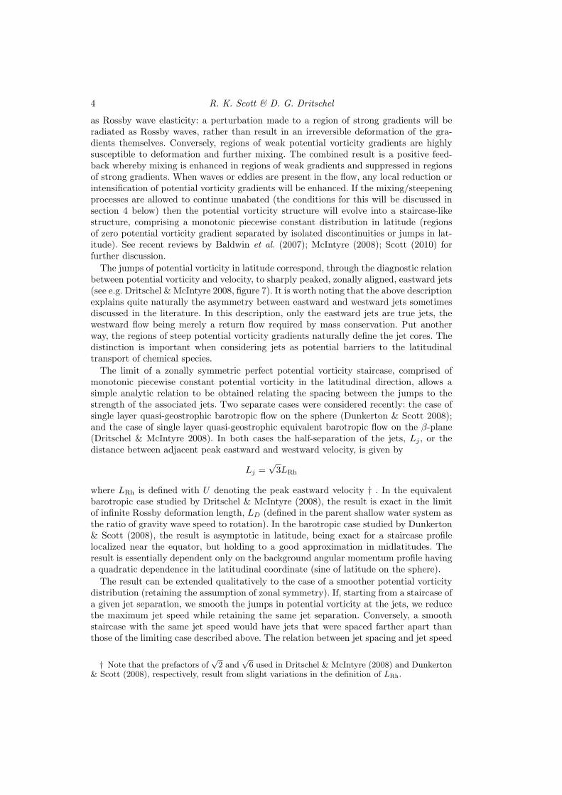
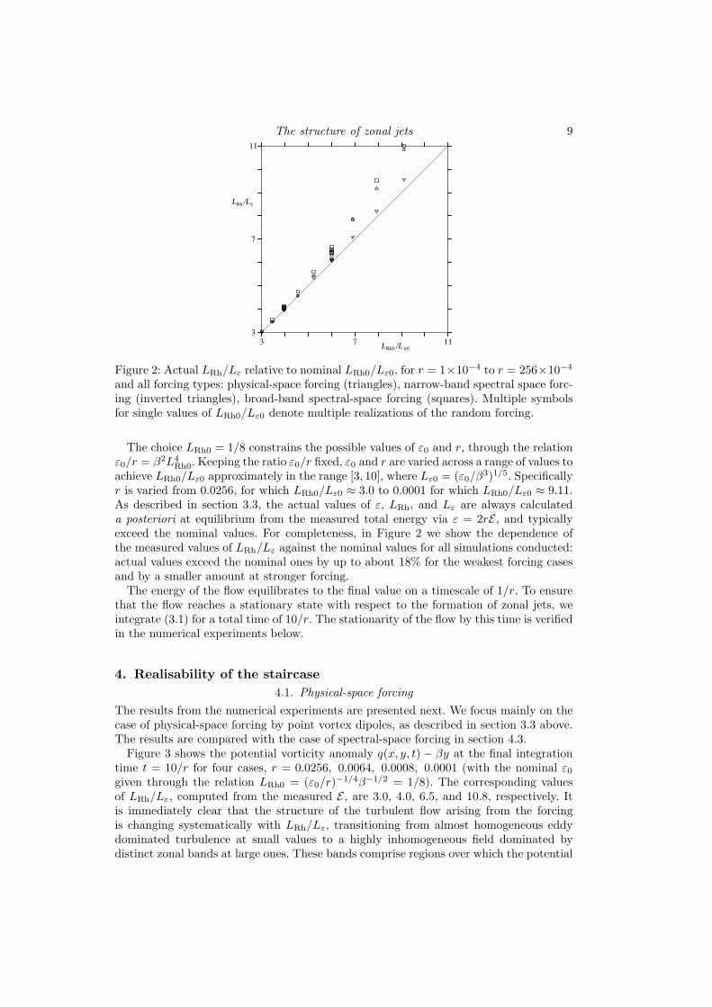
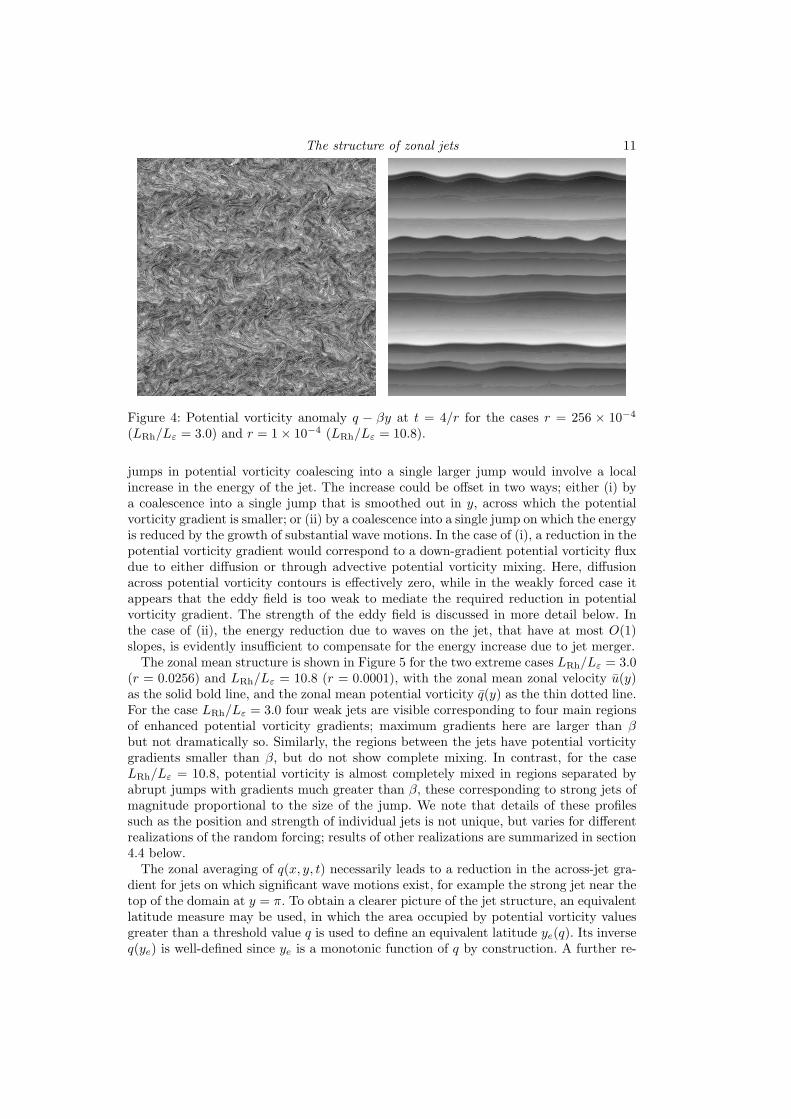
To illustrate that the integrations have reached statistical equilibrium, we show inFigure 4 the potential vorticity anomaly (the same fields) from the extreme cases r =0.0256 and r = 0.0001 at the earlier time t = 4/r. The fields are not only qualitativelysimilar to their counterparts at t = 10/r, but are also similar in many details. Forexample, the “ghost jets” just visible in the large r case are in approximately the samepositions at t = 4/r and t = 10/r; images of the fields between these times verify thatthe jets are quasi-stationary over this time interval. Similarly, the locations of the strongpotential vorticity jumps and associated jets in the small r case are almost stationary, insome cases somewhat surprisingly: the two lowermost neighbouring jets in the figure, forexample, persist throughout the entire time period and show no sign of merging into asingle large jet. In fact, such jet merger would be difficult energetically, since two small


Figure 4: Potential vorticity anomaly q − βy at t = 4/r for the cases r = 256 × 10−4

(LRh/Lε = 3.0) and r = 1× 10−4 (LRh/Lε = 10.8).

jumps in potential vorticity coalescing into a single larger jump would involve a localincrease in the energy of the jet. The increase could be offset in two ways; either (i) bya coalescence into a single jump that is smoothed out in y, across which the potentialvorticity gradient is smaller; or (ii) by a coalescence into a single jump on which the energyis reduced by the growth of substantial wave motions. In the case of (i), a reduction in thepotential vorticity gradient would correspond to a down-gradient potential vorticity fluxdue to either diffusion or through advective potential vorticity mixing. Here, diffusionacross potential vorticity contours is effectively zero, while in the weakly forced case itappears that the eddy field is too weak to mediate the required reduction in potentialvorticity gradient. The strength of the eddy field is discussed in more detail below. Inthe case of (ii), the energy reduction due to waves on the jet, that have at most O(1)slopes, is evidently insufficient to compensate for the energy increase due to jet merger.

The zonal mean structure is shown in Figure 5 for the two extreme cases LRh/Lε = 3.0(r = 0.0256) and LRh/Lε = 10.8 (r = 0.0001), with the zonal mean zonal velocity u(y)as the solid bold line, and the zonal mean potential vorticity q(y) as the thin dotted line.For the case LRh/Lε = 3.0 four weak jets are visible corresponding to four main regionsof enhanced potential vorticity gradients; maximum gradients here are larger than βbut not dramatically so. Similarly, the regions between the jets have potential vorticitygradients smaller than β, but do not show complete mixing. In contrast, for the caseLRh/Lε = 10.8, potential vorticity is almost completely mixed in regions separated byabrupt jumps with gradients much greater than β, these corresponding to strong jets ofmagnitude proportional to the size of the jump. We note that details of these profilessuch as the position and strength of individual jets is not unique, but varies for differentrealizations of the random forcing; results of other realizations are summarized in section4.4 below.

The zonal averaging of q(x, y, t) necessarily leads to a reduction in the across-jet gra-dient for jets on which significant wave motions exist, for example the strong jet near thetop of the domain at y = π. To obtain a clearer picture of the jet structure, an equivalentlatitude measure may be used, in which the area occupied by potential vorticity valuesgreater than a threshold value q is used to define an equivalent latitude ye(q). Its inverseq(ye) is well-defined since ye is a monotonic function of q by construction. A further re-


0−π

y

u/U−15

π

0

15−3 3

−1 0 1q/βπ

0−π

y

u/U−15

π

0

15−3 3

−1 0 1q/βπ

Figure 5: u(y), q(y) and q(ye) at t = 10/r for the cases r = 256× 10−4 (LRh/Lε = 3.0)and r = 1 × 10−4 (LRh/Lε = 10.8, corresponding to Fig. 3a,d. Velocities are scaled byU =

√ε0/r.

finement is used here, which considers only the potential vorticity associated with opencontours, that is, contours that span, or wrap the domain in the x-direction, a procedureintroduced in Dritschel & Scott (2011) to limit the effect of strong coherent vorticesresiding between jets. The refinement is most relevant to cases (not considered here) offinite deformation radius. In the present case, the difference between ye defined by the fullpotential vorticity field and ye defined by wrapping contours only is in fact very small;we retain the latter calculation for consistency with a companion paper considering thecase L−1

D > 0.The equivalent latitude based measure q(ye) is shown in Figure 5 by the thin continuous

lines. For the case of LRh/Lε = 3.0 there is no appreciable difference between it andthe zonal mean q(y). For the case LRh/Lε = 10.8, the quantity q(ye) in places betterillustrates the sharpness of the potential vorticity jumps associated with the jets, forexample, at the jet just below y = π, or around y = 0, π/3, −π/2, which exhibit neardiscontinuities in q(ye). For nearly straight jets the difference between q(y) and q(ye) isof course minimal.

As a final remark, it is worth noting the irregularity of the jet structure in the caseLRh/Lε = 10.8, which may be characterized by three strong jets with weaker jets existingon the flanks of the stronger ones. Their precise locations determine their directions: thejet near y = 0 has a local maximum in velocity that is, however, negative in the rest frame.In contrast, the jet near y = −3π/4 is a positive local maximum near the global maximumjust to the north. The velocity profile between the two maxima has an approximatelyparabolic profile in y (since the potential vorticity is nearly constant) and the doublepeak structure is not dissimilar to the structure of the superrotating equatorial jet onJupiter.

4.2. Eddy-jet decompositionTo examine in more detail the structure of the jets and that of the turbulent background,we make a simple decomposition of the potential vorticity field into jet and eddy com-


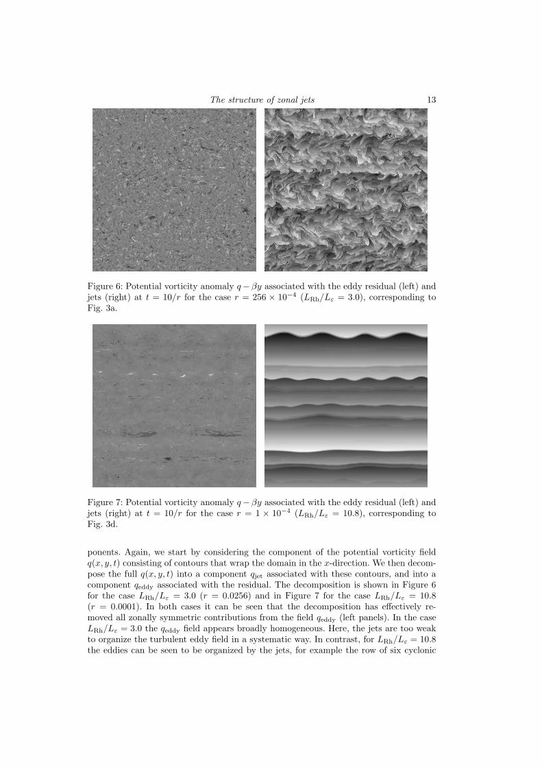
Figure 6: Potential vorticity anomaly q−βy associated with the eddy residual (left) andjets (right) at t = 10/r for the case r = 256 × 10−4 (LRh/Lε = 3.0), corresponding toFig. 3a.

Figure 7: Potential vorticity anomaly q−βy associated with the eddy residual (left) andjets (right) at t = 10/r for the case r = 1 × 10−4 (LRh/Lε = 10.8), corresponding toFig. 3d.

ponents. Again, we start by considering the component of the potential vorticity fieldq(x, y, t) consisting of contours that wrap the domain in the x-direction. We then decom-pose the full q(x, y, t) into a component qjet associated with these contours, and into acomponent qeddy associated with the residual. The decomposition is shown in Figure 6for the case LRh/Lε = 3.0 (r = 0.0256) and in Figure 7 for the case LRh/Lε = 10.8(r = 0.0001). In both cases it can be seen that the decomposition has effectively re-moved all zonally symmetric contributions from the field qeddy (left panels). In the caseLRh/Lε = 3.0 the qeddy field appears broadly homogeneous. Here, the jets are too weakto organize the turbulent eddy field in a systematic way. In contrast, for LRh/Lε = 10.8the eddies can be seen to be organized by the jets, for example the row of six cyclonic


−2

k

3210−10

−6

2

logE

logk

eddy

full

jet

−4

−2

k

3210−10

−6

2

logE

logk

eddy

full

jet

−4

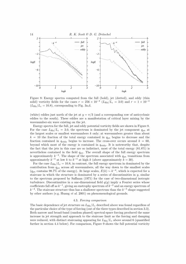
Figure 8: Energy spectra computed from the full (bold), jet (dotted), and eddy (thinsolid) vorticity fields for the cases r = 256 × 10−4 (LRh/Lε = 3.0) and r = 1 × 10−4

(LRh/Lε = 10.8), corresponding to Fig. 3a,d.

(white) eddies just north of the jet at y = π/3 (and a corresponding row of anticycloniceddies to the south). These eddies are a manifestation of critical layer mixing by thewavenumber-six wave existing on the jet.

Energy spectra for the full, jet and eddy potential vorticity fields are shown in Figure 8.For the case LRh/Lε = 3.0, the spectrum is dominated by the jet component qjet atthe largest scales or smallest wavenumbers k only; at wavenumbers greater than aboutk = 10 the fraction of the total energy contained in qjet begins to decrease and thefraction contained in qeddy begins to increase. The cross-over occurs around k = 60,beyond which most of the energy is contained in qeddy. It is noteworthy that, despitethe fact that the jets in this case are so indistinct, most of the total energy (81.8%) isnevertheless contained in the field qjet. The overall shape of the full energy spectrumis approximately k−3. The shape of the spectrum associated with qjet transitions fromapproximately k−3 at low k to k−4 at high k (above approximately k = 30).

For the case LRh/Lε = 10.8, in contrast, the full energy spectrum in dominated by thecontribution from qjet across all wavenumbers, all the way down to the smallest scales(qjet contains 98.7% of the energy). At large scales, E(k) ∼ k−4, which is expected for astaircase in which the structure is dominated by a series of discontinuities in y, similarto the spectrum proposed by Saffman (1971) for the case of two-dimensional isotropicturbulence. Discontinuities in a one-dimensional field q(y) imply a Fourier series whosecoefficients fall off as k−1, giving an enstrophy spectrum of k−2 and an energy spectrum ofk−4. The staircase structure thus has a shallower spectrum than the k−5 shape suggestedby other authors (e.g. Huang et al. 2001) on phenomenological grounds.

4.3. Forcing comparisonThe basic dependence of jet structure on LRh/Lε described above was found regardless ofthe particular choice of the type of forcing (out of the three types described in section 3.3).Both narrow and broad-band (random phased) spectral-space forcing produced the sameincrease in jet strength and approach to the staircase limit as the forcing and dampingwere reduced, with distinct staircasing appearing for LRh/Lε above around 6 (quantifiedfurther in section 4.4 below). For comparison, Figure 9 shows the full potential vorticity


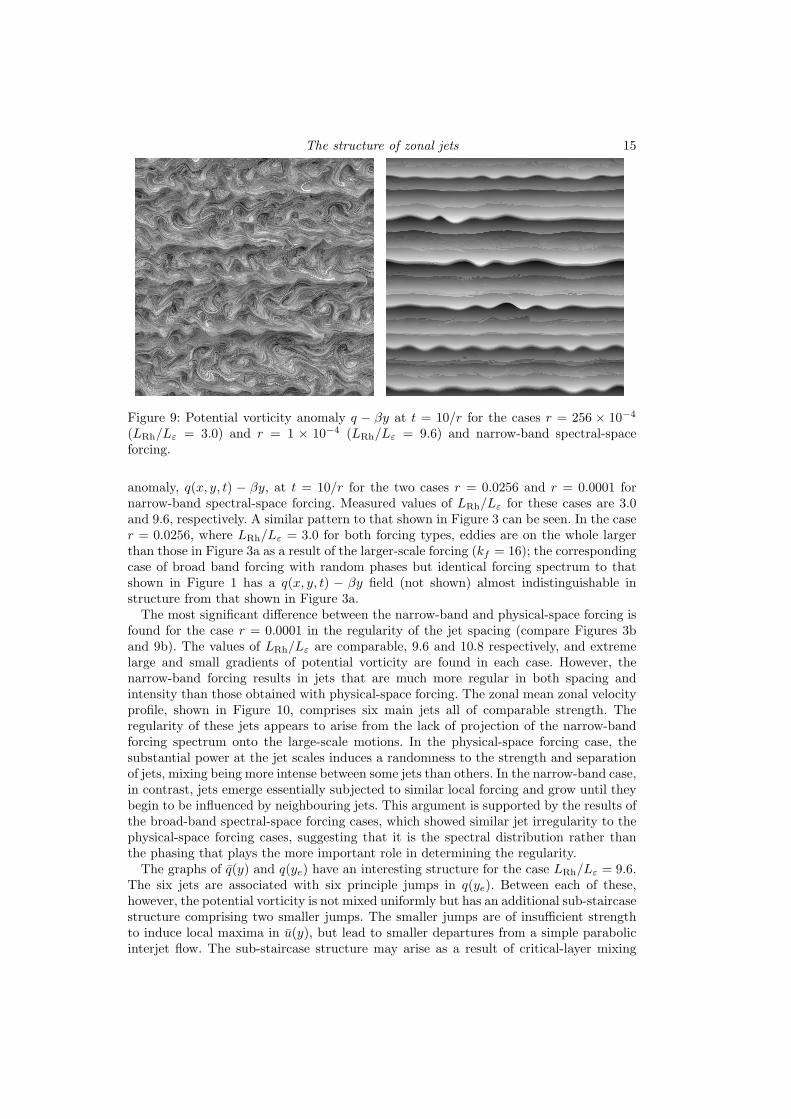
Figure 9: Potential vorticity anomaly q − βy at t = 10/r for the cases r = 256 × 10−4

(LRh/Lε = 3.0) and r = 1 × 10−4 (LRh/Lε = 9.6) and narrow-band spectral-spaceforcing.

anomaly, q(x, y, t) − βy, at t = 10/r for the two cases r = 0.0256 and r = 0.0001 fornarrow-band spectral-space forcing. Measured values of LRh/Lε for these cases are 3.0and 9.6, respectively. A similar pattern to that shown in Figure 3 can be seen. In the caser = 0.0256, where LRh/Lε = 3.0 for both forcing types, eddies are on the whole largerthan those in Figure 3a as a result of the larger-scale forcing (kf = 16); the correspondingcase of broad band forcing with random phases but identical forcing spectrum to thatshown in Figure 1 has a q(x, y, t) − βy field (not shown) almost indistinguishable instructure from that shown in Figure 3a.

The most significant difference between the narrow-band and physical-space forcing isfound for the case r = 0.0001 in the regularity of the jet spacing (compare Figures 3band 9b). The values of LRh/Lε are comparable, 9.6 and 10.8 respectively, and extremelarge and small gradients of potential vorticity are found in each case. However, thenarrow-band forcing results in jets that are much more regular in both spacing andintensity than those obtained with physical-space forcing. The zonal mean zonal velocityprofile, shown in Figure 10, comprises six main jets all of comparable strength. Theregularity of these jets appears to arise from the lack of projection of the narrow-bandforcing spectrum onto the large-scale motions. In the physical-space forcing case, thesubstantial power at the jet scales induces a randomness to the strength and separationof jets, mixing being more intense between some jets than others. In the narrow-band case,in contrast, jets emerge essentially subjected to similar local forcing and grow until theybegin to be influenced by neighbouring jets. This argument is supported by the results ofthe broad-band spectral-space forcing cases, which showed similar jet irregularity to thephysical-space forcing cases, suggesting that it is the spectral distribution rather thanthe phasing that plays the more important role in determining the regularity.

The graphs of q(y) and q(ye) have an interesting structure for the case LRh/Lε = 9.6.The six jets are associated with six principle jumps in q(ye). Between each of these,however, the potential vorticity is not mixed uniformly but has an additional sub-staircasestructure comprising two smaller jumps. The smaller jumps are of insufficient strengthto induce local maxima in u(y), but lead to smaller departures from a simple parabolicinterjet flow. The sub-staircase structure may arise as a result of critical-layer mixing


0−π

y

u/U−15

π

0

15−3 3

−1 0 1q/βπ

0−π

y

u/U−15

π

0

15−3 3

−1 0 1q/βπ

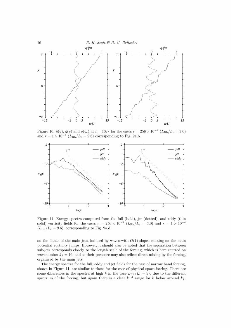
Figure 10: u(y), q(y) and q(ye) at t = 10/r for the cases r = 256× 10−4 (LRh/Lε = 3.0)and r = 1× 10−4 (LRh/Lε = 9.6) corresponding to Fig. 9a,b.

−2

k

3210−10

−6

2

logE

logk

eddy

full

jet

−4

−2

k

3210−10

−6

2

logE

logk

eddy

full

jet

−4

Figure 11: Energy spectra computed from the full (bold), jet (dotted), and eddy (thinsolid) vorticity fields for the cases r = 256 × 10−4 (LRh/Lε = 3.0) and r = 1 × 10−4

(LRh/Lε = 9.6), corresponding to Fig. 9a,d.

on the flanks of the main jets, induced by waves with O(1) slopes existing on the mainpotential vorticity jumps. However, it should also be noted that the separation betweensub-jets corresponds closely to the length scale of the forcing, which is here centred onwavenumber kf = 16, and so their presence may also reflect direct mixing by the forcing,organized by the main jets.

The energy spectra for the full, eddy and jet fields for the case of narrow band forcing,shown in Figure 11, are similar to those for the case of physical space forcing. There aresome differences in the spectra at high k in the case LRh/Lε = 9.6 due to the differentspectrum of the forcing, but again there is a clear k−4 range for k below around kf .


q/βπ0

−π

y

π

0

−1 1

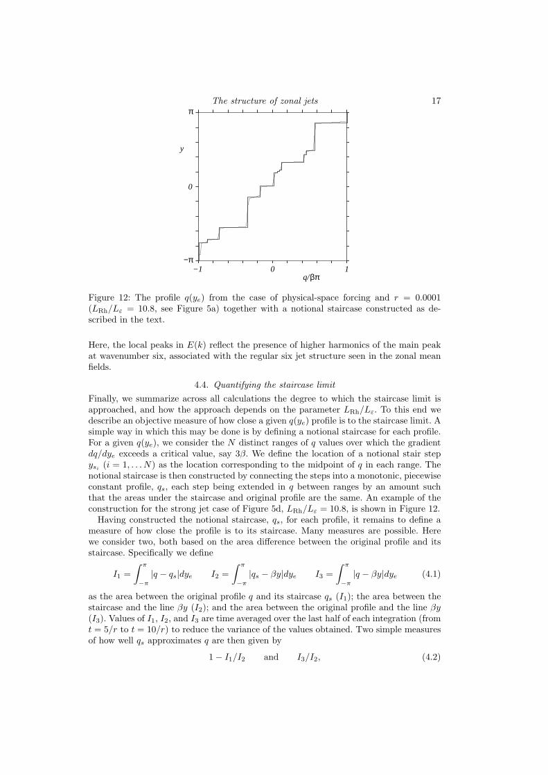
Figure 12: The profile q(ye) from the case of physical-space forcing and r = 0.0001(LRh/Lε = 10.8, see Figure 5a) together with a notional staircase constructed as de-scribed in the text.

Here, the local peaks in E(k) reflect the presence of higher harmonics of the main peakat wavenumber six, associated with the regular six jet structure seen in the zonal meanfields.

4.4. Quantifying the staircase limitFinally, we summarize across all calculations the degree to which the staircase limit isapproached, and how the approach depends on the parameter LRh/Lε. To this end wedescribe an objective measure of how close a given q(ye) profile is to the staircase limit. Asimple way in which this may be done is by defining a notional staircase for each profile.For a given q(ye), we consider the N distinct ranges of q values over which the gradientdq/dye exceeds a critical value, say 3β. We define the location of a notional stair stepysi (i = 1, . . . N) as the location corresponding to the midpoint of q in each range. Thenotional staircase is then constructed by connecting the steps into a monotonic, piecewiseconstant profile, qs, each step being extended in q between ranges by an amount suchthat the areas under the staircase and original profile are the same. An example of theconstruction for the strong jet case of Figure 5d, LRh/Lε = 10.8, is shown in Figure 12.

Having constructed the notional staircase, qs, for each profile, it remains to define ameasure of how close the profile is to its staircase. Many measures are possible. Herewe consider two, both based on the area difference between the original profile and itsstaircase. Specifically we define

I1 =∫ π

−π

|q − qs|dye I2 =∫ π

−π

|qs − βy|dye I3 =∫ π

−π

|q − βy|dye (4.1)

as the area between the original profile q and its staircase qs (I1); the area between thestaircase and the line βy (I2); and the area between the original profile and the line βy(I3). Values of I1, I2, and I3 are time averaged over the last half of each integration (fromt = 5/r to t = 10/r) to reduce the variance of the values obtained. Two simple measuresof how well qs approximates q are then given by

1− I1/I2 and I3/I2, (4.2)


2 11LRh /Lε

0

1

2 11LRh /Lε

0

1

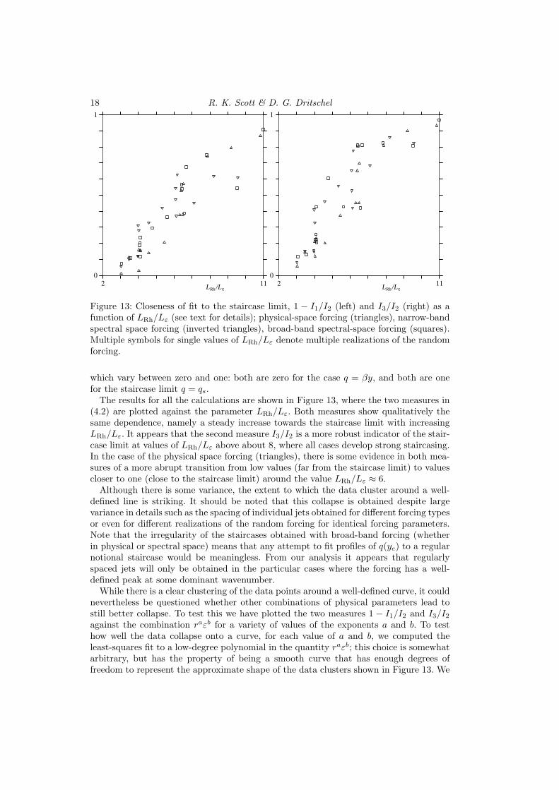
Figure 13: Closeness of fit to the staircase limit, 1 − I1/I2 (left) and I3/I2 (right) as afunction of LRh/Lε (see text for details); physical-space forcing (triangles), narrow-bandspectral space forcing (inverted triangles), broad-band spectral-space forcing (squares).Multiple symbols for single values of LRh/Lε denote multiple realizations of the randomforcing.

which vary between zero and one: both are zero for the case q = βy, and both are onefor the staircase limit q = qs.

The results for all the calculations are shown in Figure 13, where the two measures in(4.2) are plotted against the parameter LRh/Lε. Both measures show qualitatively thesame dependence, namely a steady increase towards the staircase limit with increasingLRh/Lε. It appears that the second measure I3/I2 is a more robust indicator of the stair-case limit at values of LRh/Lε above about 8, where all cases develop strong staircasing.In the case of the physical space forcing (triangles), there is some evidence in both mea-sures of a more abrupt transition from low values (far from the staircase limit) to valuescloser to one (close to the staircase limit) around the value LRh/Lε ≈ 6.

Although there is some variance, the extent to which the data cluster around a well-defined line is striking. It should be noted that this collapse is obtained despite largevariance in details such as the spacing of individual jets obtained for different forcing typesor even for different realizations of the random forcing for identical forcing parameters.Note that the irregularity of the staircases obtained with broad-band forcing (whetherin physical or spectral space) means that any attempt to fit profiles of q(ye) to a regularnotional staircase would be meaningless. From our analysis it appears that regularlyspaced jets will only be obtained in the particular cases where the forcing has a well-defined peak at some dominant wavenumber.

While there is a clear clustering of the data points around a well-defined curve, it couldnevertheless be questioned whether other combinations of physical parameters lead tostill better collapse. To test this we have plotted the two measures 1 − I1/I2 and I3/I2against the combination raεb for a variety of values of the exponents a and b. To testhow well the data collapse onto a curve, for each value of a and b, we computed theleast-squares fit to a low-degree polynomial in the quantity raεb; this choice is somewhatarbitrary, but has the property of being a smooth curve that has enough degrees offreedom to represent the approximate shape of the data clusters shown in Figure 13. We


−0.5 0.0a

0.0

0.1

b

−0.5 0.0a

0.0

0.1

b

−0.5 0.0a

0.0

0.1

b−0.5 0.0

a

0.0

0.1

b

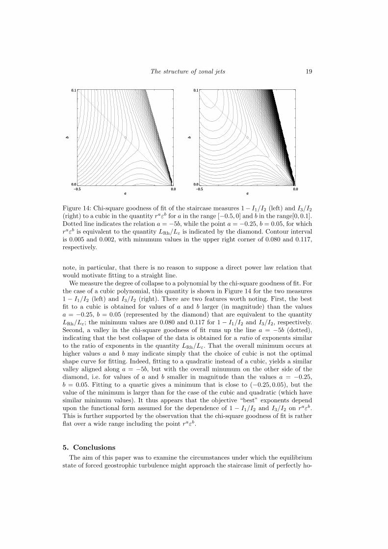
Figure 14: Chi-square goodness of fit of the staircase measures 1− I1/I2 (left) and I3/I2(right) to a cubic in the quantity raεb for a in the range [−0.5, 0] and b in the range[0, 0.1].Dotted line indicates the relation a = −5b, while the point a = −0.25, b = 0.05, for whichraεb is equivalent to the quantity LRh/Lε is indicated by the diamond. Contour intervalis 0.005 and 0.002, with minumum values in the upper right corner of 0.080 and 0.117,respectively.

note, in particular, that there is no reason to suppose a direct power law relation thatwould motivate fitting to a straight line.

We measure the degree of collapse to a polynomial by the chi-square goodness of fit. Forthe case of a cubic polynomial, this quantity is shown in Figure 14 for the two measures1 − I1/I2 (left) and I3/I2 (right). There are two features worth noting. First, the bestfit to a cubic is obtained for values of a and b larger (in magnitude) than the valuesa = −0.25, b = 0.05 (represented by the diamond) that are equivalent to the quantityLRh/Lε; the minimum values are 0.080 and 0.117 for 1 − I1/I2 and I3/I2, respectively.Second, a valley in the chi-square goodness of fit runs up the line a = −5b (dotted),indicating that the best collapse of the data is obtained for a ratio of exponents similarto the ratio of exponents in the quantity LRh/Lε. That the overall minimum occurs athigher values a and b may indicate simply that the choice of cubic is not the optimalshape curve for fitting. Indeed, fitting to a quadratic instead of a cubic, yields a similarvalley aligned along a = −5b, but with the overall minumum on the other side of thediamond, i.e. for values of a and b smaller in magnitude than the values a = −0.25,b = 0.05. Fitting to a quartic gives a minimum that is close to (−0.25, 0.05), but thevalue of the minimum is larger than for the case of the cubic and quadratic (which havesimilar minimum values). It thus appears that the objective “best” exponents dependupon the functional form assumed for the dependence of 1 − I1/I2 and I3/I2 on raεb.This is further supported by the observation that the chi-square goodness of fit is ratherflat over a wide range including the point raεb.

5. ConclusionsThe aim of this paper was to examine the circumstances under which the equilibrium

state of forced geostrophic turbulence might approach the staircase limit of perfectly ho-


mogenized zones of potential vorticity separated by sharp fronts, as studied recently byDritschel & McIntyre (2008) and Dunkerton & Scott (2008). The question is of interestin part because of the existence of the simple analytic result relating jet separation to jetstrength in the staircase limit, as reviewed in section 2. More importantly, however, it isof interest because the steepness of potential vorticity gradients in jet cores is expected toplay a key role in governing lateral transport across the jets. The latter issue is relevantto questions concerning, for example, the transport of chemical species between the tro-posphere and stratosphere across the subtropical jet, or across the winter stratosphericpolar vortex edge, as well as the lateral transport of heat, momentum, and salinity in theoceans. Understanding the physical parameters that control potential vorticity gradientsin jet cores is therefore central to understanding many aspects of the global atmosphericand oceanic circulations.

The numerical experiments reported in section 4 illustrate that the approach to astaircase-like distribution of potential vorticity can be described effectively by a singlenon-dimensional parameter, expressible as the ratio of two familiar length scales LRh/Lε.The simple result is that the staircase limit is approached for large LRh/Lε. For a varietyof forcing types, well-defined staircase distributions (strong jets) are robustly producedfor LRh/Lε ∼ O(10), whereas for LRh/Lε ∼ O(1) no clear staircasing occurs. Further,there appears to be no limit to the degree to which the staircase limit is approached:potential vorticity gradients between jets are essentially zero, while gradients in the jetcores are limited only by the numerical discretization. These results have been obtainedfor three qualitatively different types of forcing mechanism (including the commonlyused band-limited spectral space forcing) suggesting that they are robust to details ofthe forcing and its spectrum. We note also that we have observed a similar dependenceon LRh/Lε in similar experiments using a standard pseudo-spectral model (not shown),albeit at lower resolution than the results presented here.

The observed dependence on LRh/Lε appears plausible on simple physical grounds.For a given total energy of the system, strong forcing (large Lε) produces eddies withpotential vorticity anomalies that are large compared to the largest possible jump acrossa jet. In this case eddies may interact strongly with jet cores causing mixing across themand preventing potential vorticity gradients from intensifying unhindered. In the weakforcing case, on the other hand, the eddy potential vorticity anomalies are always muchweaker than the potential vorticity jumps that develop between mixing zones. As wasshown in Dritschel & McIntyre (2008), it is very difficult for an eddy to penetrate a jetwhose potential vorticity jump is greater than the eddy intensity. In part, this is becausethe eddy is not strong enough to withstand the strong shear in the region of the jet core,and so will be strongly deformed and ultimately dissipated by small-scale processes. Inpart, it is due to the dynamical resilience of the potential vorticity jump itself.

To quantify this, we analysed the maximum vorticity anomalies associated with thejet and eddy part of the vorticity field, making use of the decomposition described insection 4.2. The maximum jet vorticity anomaly increases with LRh/Lε, from around23 at LRh/Lε = 3.0 to around 42 at LRh/Lε = 10.8, larger values being associatedwith larger departures from βy for cases closer to the staircase limit. In contrast, themaximum eddy vorticity decreases with LRh/Lε from around 36 at LRh/Lε = 3.0 to 7at LRh/Lε = 10.8. In the case of LRh/Lε = 10.8, therefore, the eddy field is far too weakto be able to cause any mixing across the jets, yet is sufficient to maintain the weakgradients in between them. The crossover point, for which the jet and eddy vorticitymaxima are comparable, occurs at a value of LRh/Lε ≈ 5, consistent with the onset ofstrong jets observed in Figure 13.

An important point to note is that, in our view, it is the strength of the forcing and not


the strength of the bottom friction which is crucial in controlling the emergence of strongjets. This is in contrast both to the recent work of Berloff et al. (2011), who consideredthe effect of friction in baroclinicly forced turbulence, and to the phenomenological ar-guments of Vallis (2006), who discussed the influence of a parameter similar to LRh/Lε

on the halting of the inverse cascade by friction. Friction is here only needed to achievea stationary state, but does not play an active role in controlling the extent of staircasedevelopment. Indeed, in variations of the numerical experiments shown here in whichbottom friction is absent and in which the energy is allowed to increase linearly, a similardependence of the jet strength on the instantaneous value of LRh/Lε is found, which maynow be considered as depending on β, ε, and the total energy E (a similar conclusion wasfound in a study of undamped topographic forcing by Scott & Tissier 2012).

An interesting additional feature of the experiments reported above is the presence onthe jets of persistent waves with O(1) slopes, even in cases of extremely weak forcing.Preliminary analysis suggests that these waves arise in such a way as to maintain theflow in a state of marginal stability in the presence of a potential vorticity distributionthat is weakly non-monotonic in the north-south direction. A full analysis of these wavesand the origin of weakly non-monotonic potential vorticity will be considered in futurework.

The model used in the present study is arguably the simplest possible model thatcaptures the two main dynamical processes involved: turbulent mixing and Rossby wavepropagation. The results should therefore be interpreted with appropriate caution. Wenote that even the relatively simple extension to a finite deformation radius greatly in-creases the complexity of the problem, since the relative magnitudes of three lengthscales must be considered. Further, the equilibrium states obtained, typically comprisingjets that are highly undular coexisting with strong coherent vortices, are much harderto classify than the relatively straight jets obtained above. Further extensions to three-dimensional quasi-geostrophic flows will additionally require a more careful considerationof the different processes that might act as an eddy forcing (for example, internal baro-clinic instability driven by large-scale heating, or convective penetration at small scales)and how these should be represented in the model; the latter remains a formidable chal-lenge.

REFERENCES

Baldwin, M. P., Rhines, P. B., Huang, H.-P. & McIntyre, M. E. 2007 The jet-streamconundrum. Science 315, 467–468.

Berloff, P., Karabasov, S., Farrar, J. T. & Kamenkovich, I. 2011 On latency of multiplezonal jets in the oceans. J. Fluid Mech. 686, 534–567.

Dritschel, D. G. 1989 Contour dynamics and contour surgery: numerical algorithms for ex-tended, high-resolution modelling of vortex dynamics in two-dimensional, inviscid, incom-pressible flows. Computer Phys. Rep. 10, 78–146.

Dritschel, D. G. & Ambaum, M. H. P. 1997 A contour-advective semi-Lagrangian numericalalgorithm for simulating fine-scale conservative dynamical fields. Q. J. Roy. Meteorol. Soc.123, 1097–1130.

Dritschel, D. G. & Fontane, J. 2010 The clam algorithm: combined lagrangian advectionmethod. J. Comp. Phys. 229, 5408–5417.

Dritschel, D. G. & McIntyre, M. E. 2008 Multiple jets as PV staircases: the Phillips effectand the resilience of eddy-transport barriers. J. Atmos. Sci 65, 855–874.

Dritschel, D. G. & Scott, R. K. 2009 On the simulation of nearly inviscid two-dimensionalturbulence. J. Comp. Phys. 228, 2707–2711.


Dritschel, D. G. & Scott, R. K. 2011 Jet sharpening by turbulent mixing. Phil. Tran. Roy.Soc. A 369, 754–770.

Dunkerton, T. J. & Scott, R. K. 2008 A barotropic model of the angular momentumconserving potential vorticity staircase in spherical geometry. J. Atmos. Sci. 65, 1105–1136.

Fontane, J. & Dritschel, D. 2009 The HyperCASL Algorithm: a new approach to the nu-merical simulation of geophysical flows. J. Comput. Phys. 228, 6411–6425.

Galperin, B., Nakano, H., Huang, H.-P. & Sukoriansky, S. 2004 The ubiquitous zonal jetsin the atmospheres of giant planets and Earth’s oceans. Geophys. Res. Lett. 31, L13303.

Huang, H.-P., Galperin, B. & Sukoriansky, S. 2001 Anisotropic spectra in two-dimensionalturbulence on the surface of a rotating sphere. Phys. Fluids 13, 225–240.

Maltrud, M. E. & Vallis, G. K. 1991 Energy spectra and coherent structures in forcedtwo-dimensional and beta-plane turbulence. J. Fluid Mech. 228, 321–342.

Marcus, P. S. 1993 Jupiter’s great red spot and other vortices. Ann. Rev. Astron. Astrophys.31, 523–573.

McIntyre, M. E. 1982 How well do we understand the dynamics of stratospheric warmings?J. Meteorol. Soc. Japan 60, 37–65, special issue in commemoration of the centennial of theMeteorological Society of Japan, ed. K. Ninomiya.

McIntyre, M. E. 2008 Potential-vorticity inversion and the wave–turbulence jigsaw: somerecent clarifications. Adv. Geosci. 15, 47–56.

Panetta, R. L. 1993 Zonal jets in wide baroclinically unstable regions: persistence and scaleselection. J Atmos Sci 50, 2073–2106.

Peltier, W. R. & Stuhne, G. R. 2002 The upscale turbulent cascade: shear layers, cyclonesand gas giant bands. In Meteorology at the Millennium (ed. R. Pierce). Academic Press,San Diego.

Phillips, O. M. 1972 Turbulence in a strongly stratified fluid — is it unstable? Deep Sea Res.19, 79–81.

Rhines, P. B. 1975 Waves and turbulence on a beta-plane. J. Fluid Mech. 69, 417–443.Saffman, P. G. 1971 On the spectrum and decay of random two-dimensional vorticity distri-

butions at large Reynolds number. Stud. Appl. Math. 50, 377–383.Scott, R. K. 2010 The structure of zonal jets in shallow water turbulence on the sphere.

IUTAM Symposium on Turbulence in the Atmosphere and Oceans; IUTAM Bookseries28, 243–252.

Scott, R. K. & Polvani, L. M. 2007 Forced-dissipative shallow water turbulence on the sphereand the atmospheric circulation of the gas planets. J. Atmos. Sci 64, 3158–3176.

Scott, R. K. & Tissier, A.-S. 2012 The generation of zonal jets by large-scale mixing. Phys.Fluids Submitted.

Sukoriansky, S., Dikovskaya, N. & Galperin, B. 2007 On the arrest of inverse energycascade and the Rhines scale. J. Atmos. Sci 64, 3312–3327.

Vallis, G. K. 2006 Atmospheric and Oceanic Fluid Dynamics. Cambridge University Press.Williams, G. P. 1978 Planetary circulations: 1. Barotropic representation of Jovian and ter-

restrial turbulence. J. Atmos. Sci. 35, 1399–1424.

The structure of zonal jets in geostrophic turbulencerks/preprints/scott_dritschel_jfm_2012.pdf ·...

Documents

Transcript of The structure of zonal jets in geostrophic turbulencerks/preprints/scott_dritschel_jfm_2012.pdf ·...