Speaking Stata Graphics:

A Collection from the Stata Journal

NICHOLAS J. COXDurham University

Department of Geography

®

A Stata Press PublicationStataCorp LPCollege Station, Texas

® Copyright c© 2014 by StataCorp LPAll rights reserved. First edition 2014

Published by Stata Press, 4905 Lakeway Drive, College Station, Texas 77845Typeset in LATEX2εPrinted in the United States of America

10 9 8 7 6 5 4 3 2 1

ISBN-10: 1-59718-144-7ISBN-13: 978-1-59718-144-0

Library of Congress Control Number: 2014936700

Copyright Statement: The Stata Journal and the contents of the supporting files (programs,datasets, and help files) are copyright c© by StataCorp LP. The contents of the supporting files(programs, datasets, and help files) may be copied or reproduced by any means whatsoever,in whole or in part, as long as any copy or reproduction includes attribution to both (1) theauthor and (2) the Stata Journal.

The articles appearing in the Stata Journal may be copied or reproduced as printed copies,in whole or in part, as long as any copy or reproduction includes attribution to both (1) theauthor and (2) the Stata Journal.

Written permission must be obtained from StataCorp if you wish to make electronic copiesof the insertions. This precludes placing electronic copies of the Stata Journal, in whole orin part, on publicly accessible websites, fileservers, or other locations where the copy may beaccessed by anyone other than the subscriber.

Users of any of the software, ideas, data, or other materials published in the Stata Journal orthe supporting files understand that such use is made without warranty of any kind, by eitherthe Stata Journal, the author, or StataCorp. In particular, there is no warranty of fitness ofpurpose or merchantability, nor for special, incidental, or consequential damages such as lossof profits. The purpose of the Stata Journal is to promote free communication among Statausers.

The Stata Journal (ISSN 1536-867X) is a publication of Stata Press. Stata, , Stata Press,Mata, , and NetCourse are registered trademarks of StataCorp LP.

Stata and Stata Press are registered trademarks with the World Intellectual Property Organi-zation of the United Nations.

LATEX2ε is a trademark of the American Mathematical Society.

Contents

Preface vii

Software notes on the original columns xiii

Graphing distributions . . . . . . . . . . . . . . . . . . . . . . . . . . . . . . . . . . . . . . . . . . . . . . . . . . . . . . . . . 1

Graphing categorical and compositional data . . . . . . . . . . . . . . . . . . . . . . . . . . . . . . . . . . . 24

Graphing agreement and disagreement. . . . . . . . . . . . . . . . . . . . . . . . . . . . . . . . . . . . . . . . . . 50

Graphing model diagnostics . . . . . . . . . . . . . . . . . . . . . . . . . . . . . . . . . . . . . . . . . . . . . . . . . . . . 71

Density probability plots . . . . . . . . . . . . . . . . . . . . . . . . . . . . . . . . . . . . . . . . . . . . . . . . . . . . . . . 98

The protean quantile plot . . . . . . . . . . . . . . . . . . . . . . . . . . . . . . . . . . . . . . . . . . . . . . . . . . . . . . 113

Smoothing in various directions . . . . . . . . . . . . . . . . . . . . . . . . . . . . . . . . . . . . . . . . . . . . . . . . 132

Graphs for all seasons . . . . . . . . . . . . . . . . . . . . . . . . . . . . . . . . . . . . . . . . . . . . . . . . . . . . . . . . . . 152

Turning over a new leaf . . . . . . . . . . . . . . . . . . . . . . . . . . . . . . . . . . . . . . . . . . . . . . . . . . . . . . . . 175

Spineplots and their kin . . . . . . . . . . . . . . . . . . . . . . . . . . . . . . . . . . . . . . . . . . . . . . . . . . . . . . . . 196

Between tables and graphs . . . . . . . . . . . . . . . . . . . . . . . . . . . . . . . . . . . . . . . . . . . . . . . . . . . . . 213

Creating and varying box plots . . . . . . . . . . . . . . . . . . . . . . . . . . . . . . . . . . . . . . . . . . . . . . . . . 234

Creating and varying box plots: Correction . . . . . . . . . . . . . . . . . . . . . . . . . . . . . . . . . . . . . 253

Paired, parallel, or profile plots for changes, correlations, and other comparisons 256

The statsby strategy . . . . . . . . . . . . . . . . . . . . . . . . . . . . . . . . . . . . . . . . . . . . . . . . . . . . . . . . . . . 275

Graphing subsets . . . . . . . . . . . . . . . . . . . . . . . . . . . . . . . . . . . . . . . . . . . . . . . . . . . . . . . . . . . . . . . 284

Transforming the time axis . . . . . . . . . . . . . . . . . . . . . . . . . . . . . . . . . . . . . . . . . . . . . . . . . . . . . 296

Axis practice, or what goes where on a graph . . . . . . . . . . . . . . . . . . . . . . . . . . . . . . . . . . . 306

Trimming to taste . . . . . . . . . . . . . . . . . . . . . . . . . . . . . . . . . . . . . . . . . . . . . . . . . . . . . . . . . . . . . . 319

Preface

The Stata Technical Bulletin was started in 1991 as a journal by and for users of thestatistical software Stata. As a Stata enthusiast, I subscribed from issue 1, startedcontributing in 1994, and became an associate editor in 1998. In 2001, a decision wasmade to transform the Bulletin into the Stata Journal, and I became one of the editors.The initial meeting setting up the journal was a working breakfast in a Boston hotel,otherwise made memorable by my being offered cottage cheese as an alternative toyogurt with my cereal. Among many other details, two suggestions followed in quicksuccession: that there should be a column in the Journal and that I should write it. Iremain gratefully aware of the compliment implied.

I settled on a title, Speaking Stata, to match both the privilege of sounding off onmy own Stata-linked preoccupations and prejudices and the purpose of explaining theuse of Stata’s language in a way that grew from, but went beyond, the excellent Statadocumentation. As a columnist, I claim no more than certain interests and points ofview; I take comfort in the simple thought that others are free to write on quite differenttopics and from quite different perspectives.

This book collects those columns published between 2004 and 2013 with a majortheme of statistical graphics. My strong interest in graphics has grown steadily out ofmy education and experience as an academic geographer and a long-standing fascinationwith geometry and spatial patterns. Despite greatly renewed attention given to graphicsover the last few decades within statistical science, I think it remains true that they aregenerally undervalued within several disciplines, but this is not the place to argue thatview in any detail. The columns also include coverage of several little-known and evensome apparently new ways of graphing data. A keen personal interest in the history ofideas, which surfaces in several columns, underlines the extent to which good ideas arepersistently reinvented, so one can never be sure.

I have received strong and consistent counsel not to attempt any serious rewriting.The columns were certainly written one at a time and are intended to be read, mostly,one at a time. Unlike Dickens, Dumas, or Dostoyevsky, I have not been writing a novelin serial installments. Nevertheless, my own interests should give some coherence to thecollection.

Learning statistics software, like learning statistics itself, can be a series of smallstruggles until enlightenment dawns and you wonder why on earth the idea appeareddifficult in the first place. While writing these columns, I have tried to be clear ratherthan clever because I know from my own experience that several ideas in Stata, althoughbeautifully simple when considered in the right way, are far from transparent at first

viii Preface

sight. Similarly, some repetitions remain in the hope that they provide reinforcementor serve the purposes of those with neither time nor inclination to read every column.

However, what is here is a little more than a straight reprinting. References to theStata manuals have been updated. A few misprints have been corrected. (“Misprint”is British for “typo”.) Notes following this Preface identify software changes sincethe columns were first produced. In any case, readers interested in identifying the mostrecent versions of any user-written programs should first use search, all within Stata.

Any writer accumulates many debts that cannot all be discharged or even acknowl-edged. William (Bill) Gould is the person who conceived of Stata and set up thecompany that maintains and develops it. StataCorp is a company that aspires to excel-lence in everything. As I discovered long ago, it is grateful even to be told of all bugsand misfeatures, down to misprints in its manuals. I remain perpetually aware that Ifollow in Bill’s footsteps and stand on his shoulders.

I have also received much patient and detailed support from many other peopleat StataCorp. Vince Wiggins has borne the brunt of most of my specific graphicsquestions over the last decade, alerted me to some subtle tricks, and made encouragingnoises throughout. Pat Branton, Lisa Gilmore, and their past and present colleagueshave accommodated most of the quirks and dilatory submissions of an author withsome strong prejudices about the English (N.B. not American) language and writinggenerally. Many in the Stata user community have asked good questions and providedmost of the answers through encounters at users’ meetings, postings on Statalist, andpublications in the Stata Technical Bulletin and the Stata Journal. My fellow EditorJoe Newton has proved a master of the timely quiet word of approbation. Variousspecific acknowledgments are recorded in individual columns, but they form a sadlyincomplete list. Although it is, as always, invidious to single out a few names, thosewho know anything of their work would want to echo further special thanks to KitBaum, Marcello Pagano, and Patrick Royston for their long-standing endeavors for theStata user community.

At Durham University, several geographical colleagues have kept me honest by pro-viding a series of statistical challenges within a fascinating variety of datasets. Ian Evansin particular has also been an appreciative Stata user for many years. The division oflabor in our collaborations that he did most of the more challenging science and I didmost of the more challenging Stata programming has proved mutually congenial. It hasbeen a special pleasure to remain in collaboration with my own PhD supervisor for over40 years.

Most personally, I dedicate this book to my wife, Irene, in recognition of all theencouragement and support she has provided over our time together.

Nicholas J. Cox

Preface ix

Note: What follows is a complete list of my publications on Stata that are mostlygraphical. As of this writing, all material published more than three years ago isfreely available at http://www.stata-journal.com in the case of the Stata Journal and athttp://www.stata.com/bookstore/individual-stata-technical-bulletin-issues/ in the caseof the Stata Technical Bulletin. Graphical tips by me have been collected within Coxand Newton (2014).

SSG indicates reprinting in this book, and 119 indicates reprinting in Cox and Newton(2014).

Cox, N. J. 1997. gr16.1: Convex hull plots. Stata Technical Bulletin 36: 2–3. Reprintedin Stata Technical Bulletin Reprints, vol. 6, pp. 25–27. College Station, TX: StataPress.

——. 1997. gr22: Binomial smoothing plot. Stata Technical Bulletin 35: 7–9. Reprintedin Stata Technical Bulletin Reprints, vol. 6, pp. 36–38. College Station, TX: StataPress.

——. 1997. gr24: Easier bar charts. Stata Technical Bulletin 36: 4–8. Reprinted inStata Technical Bulletin Reprints, vol. 6, pp. 44–50. College Station, TX: StataPress.

——. 1997. gr24.1. Easier bar charts: correction. Stata Technical Bulletin 40: 12.Reprinted in Stata Technical Bulletin Reprints, vol. 7, p. 58. College Station, TX:Stata Press.

——. 1997. gr26: Bin smoothing and summary on scatter plots. Stata TechnicalBulletin 37: 9–12. Reprinted in Stata Technical Bulletin Reprints, vol. 7, pp. 59–63.College Station, TX: Stata Press.

——. 1998. sg85: Moving summaries. Stata Technical Bulletin 44: 15–18. Reprinted inStata Technical Bulletin Reprints, vol. 8, pp. 145–149. College Station, TX: StataPress.

——. 1999. gr35: Diagnostic plots for assessing Singh-Maddala and Dagum distribu-tions fitted by MLE. Stata Technical Bulletin 48: 2–4. Reprinted in Stata TechnicalBulletin Reprints, vol. 8, pp. 72–74. College Station, TX: Stata Press.

——. 1999. gr41: Distribution function plots. Stata Technical Bulletin 51: 12–16.Reprinted in Stata Technical Bulletin Reprints, vol. 9, pp. 108–112. College Station,TX: Stata Press.

——. 1999. gr42: Quantile plots, generalized. Stata Technical Bulletin 51: 16–18.Reprinted in Stata Technical Bulletin Reprints, vol. 9, pp. 113–116. College Station,TX: Stata Press.

——. 2001. gr42.1: Quantile plots, generalized: update to Stata 7.0. Stata TechnicalBulletin 61: 10–11. Reprinted in Stata Technical Bulletin Reprints, vol. 10, pp. 55–56. College Station, TX: Stata Press.

——. 2003. Software update: gr41 1: Distribution function plots. Stata Journal 3: 211.

x Preface

——. 2003. Software update: gr41 2: Distribution function plots. Stata Journal 3: 449.

——. 2004. Software update: gr22 1: Binomial smoothing plot. Stata Journal 4: 490–491.

——. 2004. Software update: gr42 2: Quantile plots, generalized. Stata Journal 4: 97.

——. 2004. Speaking Stata: Graphing agreement and disagreement. Stata Journal 4:329–349 (SSG).

——. 2004. Speaking Stata: Graphing categorical and compositional data. Stata Jour-nal 4: 190–215 (SSG).

——. 2004. Speaking Stata: Graphing distributions. Stata Journal 4: 66–88 (SSG).

——. 2004. Speaking Stata: Graphing model diagnostics. Stata Journal 4: 449–475(SSG).

——. 2004. Stata tip 6: Inserting awkward characters in the plot. Stata Journal 4:95–96 (119).

——. 2004. Stata tip 12: Tuning the plot region aspect ratio. Stata Journal 4: 357–358(119).

——. 2004. Stata tip 15: Function graphs on the fly. Stata Journal 4: 488–489 (119).

——. 2005. Software update: gr41 3: Distribution function plots. Stata Journal 5:470–471.

——. 2005. Software update: gr42 3: Quantile plots, generalized. Stata Journal 5:470–471.

——. 2005. Speaking Stata: Density probability plots. Stata Journal 5: 259–273 (SSG).

——. 2005. Speaking Stata: The protean quantile plot. Stata Journal 5: 442–460 (SSG).

——. 2005. Speaking Stata: Smoothing in various directions. Stata Journal 5: 574–593(SSG).

——. 2005. Stata tip 21: The arrows of outrageous fortune. Stata Journal 5: 282–284(119).

——. 2005. Stata tip 24: Axis labels on two or more levels. Stata Journal 5: 469 (119).

——. 2005. Stata tip 27: Classifying data points on scatter plots. Stata Journal 5:604–606 (119).

——. 2006. Software update: gr26 1: Bin smoothing and summary on scatter plots.Stata Journal 6: 151.

——. 2006. Software update: gr42 4: Quantile plots, generalized. Stata Journal 6: 597.

——. 2006. Speaking Stata: Graphs for all seasons. Stata Journal 6: 397–419 (SSG).

——. 2007. Software update: gr0012 1: Density probability plots. Stata Journal 7:593.

Preface xi

——. 2007. Speaking Stata: Turning over a new leaf. Stata Journal 7: 413–433 (SSG).

——. 2007. Stata tip 47: Quantile–quantile plots without programming. Stata Journal7: 275–279 (119).

——. 2007. Stata tip 55: Better axis labeling for time points and time intervals. StataJournal 7: 590–592 (119).

——. 2008. Speaking Stata: Between tables and graphs. Stata Journal 8: 269–289(SSG).

——. 2008. Speaking Stata: Spineplots and their kin. Stata Journal 8: 105–121 (SSG).

——. 2008. Stata tip 59: Plotting on any transformed scale. Stata Journal 8: 142–145(119).

——. 2009. Speaking Stata: Creating and varying box plots. Stata Journal 9: 478–496(SSG).

——. 2009. Speaking Stata: Paired, parallel, or profile plots for changes, correlations,and other comparisons. Stata Journal 9: 621–639 (SSG).

——. 2009. Stata tip 76: Separating seasonal time series. Stata Journal 9: 321–326(119).

——. 2009. Stata tip 78: Going gray gracefully: Highlighting subsets and downplayingsubstrates. Stata Journal 9: 499–503 (119).

——. 2009. Stata tip 82: Grounds for grids on graphs. Stata Journal 9: 648–651 (119).

——. 2010. Software update: gr0009 1: Speaking Stata: Graphing model diagnostics.Stata Journal 10: 164 (SSG).

——. 2010. Software update: gr0021 1: Speaking Stata: Smoothing in various direc-tions. Stata Journal 10: 164 (SSG).

——. 2010. Software update: gr41 4: Distribution function plots. Stata Journal 10:164.

——. 2010. Software update: gr42 5: Quantile plots, generalized. Stata Journal 10:691–692.

——. 2010. Speaking Stata: Graphing subsets. Stata Journal 10: 670–681 (SSG).

——. 2010. Speaking Stata: The statsby strategy. Stata Journal 10: 143–151 (SSG).

——. 2011. Stata tip 102: Highlighting specific bars. Stata Journal 11: 474–477 (119).

——. 2011. Stata tip 104: Added text and title options. Stata Journal 11: 632–633(119).

——. 2012. Software update: gr42 6: Quantile plots, generalized. Stata Journal 12:167.

xii Preface

——. 2012. Speaking Stata: Axis practice, or what goes where on a graph. StataJournal 12: 549–561 (SSG).

——. 2012. Speaking Stata: Transforming the time axis. Stata Journal 12: 332–41(SSG).

——. 2013. Speaking Stata: Creating and varying box plots: Correction. Stata Journal13: 398–400 (SSG).

——. 2013. Speaking Stata: Trimming to taste. Stata Journal 13: 640–666 (SSG).

——. 2014. Stata tip 119: Expanding datasets for graphical ends. Stata Journal 14:230–235 (119).

Cox, N. J., and N. L. M. Barlow. 2008. Stata tip 62: Plotting on reversed scales. StataJournal 8: 295–298 (119).

Cox, N. J., and A. R. Brady. 1997. gr25: Spike plots for histograms, rootograms, andtime-series plots. Stata Technical Bulletin 36: 8–11. Reprinted in Stata TechnicalBulletin Reprints, vol. 6, pp. 50–54. College Station, TX: Stata Press.

——. 1997. gr25.1: Spike plots for histograms, rootograms, and time-series plots:update. Stata Technical Bulletin 40: 12. Reprinted in Stata Technical BulletinReprints, vol. 7, p. 58. College Station, TX: Stata Press.

Cox, N. J., and H. J. Newton, eds. 2014. One Hundred Nineteen Stata Tips. StataPress, College Station, TX.

Gray, J. P., and N. J. Cox. 1998. gr16.2: Corrections to condraw.ado. Stata TechnicalBulletin 41: 4. Reprinted in Stata Technical Bulletin Reprints, vol. 7, p. 58. CollegeStation, TX: Stata Press.

Royston, P., and N. J. Cox. 2005. A multivariable scatterplot smoother. Stata Journal5: 405–412.

Sasieni, P., P. Royston, and N. J. Cox. 2005. Software update: sed9 2: Symmetricnearest neighbor linear smoothers. Stata Journal 5: 285.

The Stata Journal (2004)4, Number 1, pp. 66–88 1

Speaking Stata: Graphing distributions

Nicholas J. CoxUniversity of Durham, UK

n.j.cox@durham.ac.uk

Abstract. Graphing univariate distributions is central to both statistical graphics,in general, and Stata’s graphics, in particular. Now that Stata 8 is out, a review ofofficial and user-written commands is timely. The emphasis here is on going beyondwhat is obviously and readily available, with pointers to minor and major trickeryand various user-written commands. For plotting histogram-like displays, kernel-density estimates and plots based on distribution functions or quantile functions,a large variety of choices is now available to the researcher.

Keywords: gr0003, graphics, histogram, spikeplot, dotplot, onewayplot, kdensity,distplot, qplot, skewplot, bin width, rug, density function, kernel estimation, trans-formations, logarithmic scale, root scale, intensity function, distribution function,quantile function, skewness

1 Introduction

The new graphics introduced in Stata 8 has been, by far, the most important stepforward in Stata’s graphical functionality since early releases in the mid-1980s. It is,therefore, high time that this column turned to discuss graphics directly. I intend tomake 2004 a graphic year for Speaking Stata, starting with the basic and fundamen-tal issue of graphing univariate distributions. Future columns are intended to discussgraphing categorical and compositional data, comparisons, and model diagnostics. Ineach case, the aim will be to provide an overview of Stata’s provision and to show waysto go beyond what is obviously and readily available. The emphasis will be on graphicscommands of potential interest to the largest possible cross-section of Stata users. Thushistograms clearly qualify, but justice cannot be done to details specific to analysis ofsurvival-time distributions.

The core commands for graphing distributions range from twoway kdensity andits relative kdensity through twoway histogram and its relative histogram to graph

box and graph hbox. Related but perhaps less-often used commands include dotplot,spikeplot, and those grouped as diagnostic plots.

2 Histograms, indigenous and exotic

2.1 Number of bins and bin width

With an eye to tradition, including Stata tradition, let us start the discussion withhistograms. Up until Stata 7, a histogram was the default graph type if graph was fedjust one variable. Before Stata 8, such histograms were relatively inflexible and could

2 Speaking Stata

not easily be combined with other graph types. Now we have both greater flexibilityand easier working with other types. Notable additions include the options to tune bothbin width and the start of binning, whereas previously only the number of bins couldbe controlled directly. The start of binning could be controlled indirectly by tuningxlabel() or xscale().

As every good introductory text explains, histogram construction is largely a trade-off problem in which you seek a compromise between detail and generalization or be-tween variance and bias. In doing this, you can tune either the number of bins or thebin width. Theoretical discussions concentrate on the number of bins and its relationto sample size and the kind of distribution being analyzed. However, my guess is thatpeople with their feet in application areas often find it natural to think in terms of asensible bin width for the variables they have, bearing in mind measurement issues andthe magnitude of important or interpretable differences. Whatever your preference, youcan now do it either way.

2.2 Varying bin widths

However, one feature that remains wired in histogram commands in Stata 8 is a restric-tion to bins of equal width. No doubt this is often very sensible whenever the originaldata are available, but there are occasions on which you might want to break this rule.Let us drill down to some first principles here.

Recall that the idea behind histograms is that the area of each bar represents thefraction of a frequency (probability) distribution within each bin (or class, or interval).Among many books explaining histograms, Freedman, Pisani, and Purves (1978) is anoutstanding introductory text that strongly emphasizes the area principle. It is not partof the definition that all bins have the same width, but rather that what is shown on thevertical axis is, or is proportional to, probability density. Frequency density qualifies,as does frequency if all bins have the same width.

In practice, the choice of bin width is often a little arbitrary. If the variable is discrete,a width of 1 is clearly a natural choice. Even then, discrete variables may require somegrouping into bins wider than 1. If the variable is number of lifetime sexual partners,the tail (apparently) stretches into very large numbers, and some grouping may bedesired. With continuous variables especially, there is always some arbitrariness. Manyresearchers are most reluctant to compound that by varying the width of the intervals.To do so would complicate the interpretation of the histogram, it might be argued, byany variations in the way the bars were produced. Or, to put it another way, equalwidths are relatively simple, and any kind of complexity beyond them needs to bejustified.

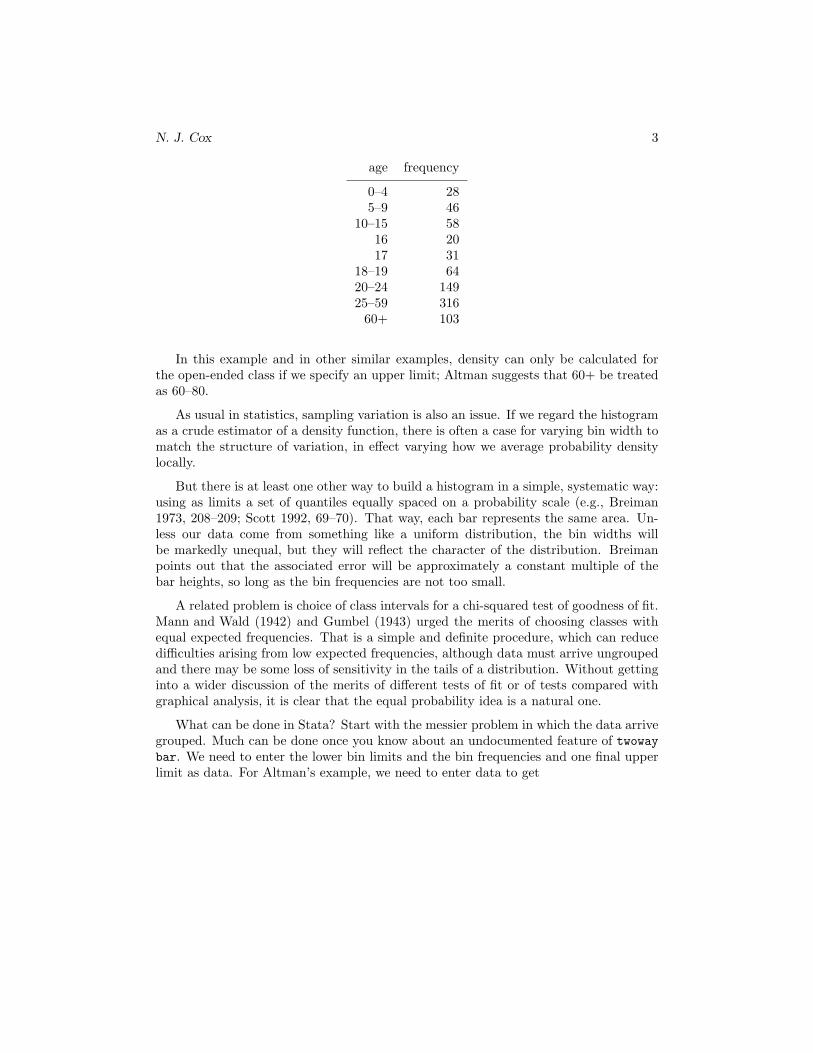
Despite all that, sometimes the data come grouped into irregular intervals, and theresearcher has little or no choice because the raw data may be difficult or impossible toaccess. Sometimes there is an underlying confidentiality issue. Nevertheless, researchersmay still want a histogram, which should be correctly drawn with density, not frequency,on the vertical axis. For example, Altman (1991, 25) gives the ages of 815 road accidentcasualties for the London Borough of Harrow in 1985:

N. J. Cox 3

age frequency

0–4 285–9 46

10–15 5816 2017 31

18–19 6420–24 14925–59 31660+ 103

In this example and in other similar examples, density can only be calculated forthe open-ended class if we specify an upper limit; Altman suggests that 60+ be treatedas 60–80.

As usual in statistics, sampling variation is also an issue. If we regard the histogramas a crude estimator of a density function, there is often a case for varying bin width tomatch the structure of variation, in effect varying how we average probability densitylocally.

But there is at least one other way to build a histogram in a simple, systematic way:using as limits a set of quantiles equally spaced on a probability scale (e.g., Breiman1973, 208–209; Scott 1992, 69–70). That way, each bar represents the same area. Un-less our data come from something like a uniform distribution, the bin widths willbe markedly unequal, but they will reflect the character of the distribution. Breimanpoints out that the associated error will be approximately a constant multiple of thebar heights, so long as the bin frequencies are not too small.

A related problem is choice of class intervals for a chi-squared test of goodness of fit.Mann and Wald (1942) and Gumbel (1943) urged the merits of choosing classes withequal expected frequencies. That is a simple and definite procedure, which can reducedifficulties arising from low expected frequencies, although data must arrive ungroupedand there may be some loss of sensitivity in the tails of a distribution. Without gettinginto a wider discussion of the merits of different tests of fit or of tests compared withgraphical analysis, it is clear that the equal probability idea is a natural one.

What can be done in Stata? Start with the messier problem in which the data arrivegrouped. Much can be done once you know about an undocumented feature of twowaybar. We need to enter the lower bin limits and the bin frequencies and one final upperlimit as data. For Altman’s example, we need to enter data to get

4 Speaking Stata

. list age freq

age freq

1. 0 282. 5 463. 10 584. 16 205. 17 31

6. 18 647. 20 1498. 25 3169. 60 10310. 80 .

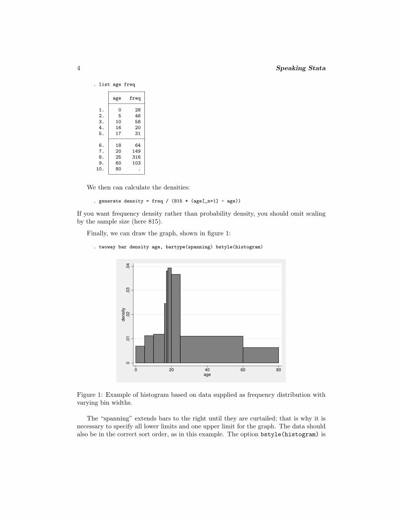
We then can calculate the densities:

. generate density = freq / (815 * (age[_n+1] - age))

If you want frequency density rather than probability density, you should omit scalingby the sample size (here 815).

Finally, we can draw the graph, shown in figure 1:

. twoway bar density age, bartype(spanning) bstyle(histogram)

0.0

1.0

2.0

3.0

4density

0 20 40 60 80age

Figure 1: Example of histogram based on data supplied as frequency distribution withvarying bin widths.

The “spanning” extends bars to the right until they are curtailed; that is why it isnecessary to specify all lower limits and one upper limit for the graph. The data shouldalso be in the correct sort order, as in this example. The option bstyle(histogram) is

N. J. Cox 5

not compulsory, and you might like to check other possibilities. You might need to addthe option yscale(range(0)) if twoway bar does not automatically start bars at 0.

Turning to the more elegant problem, a user-written program for equal-probabilityhistograms can be described and, if desired, downloaded from the Statistical SoftwareComponents (SSC) archive by using the ssc command; see [R] ssc:

. ssc describe eqprhistogram

. ssc install eqprhistogram

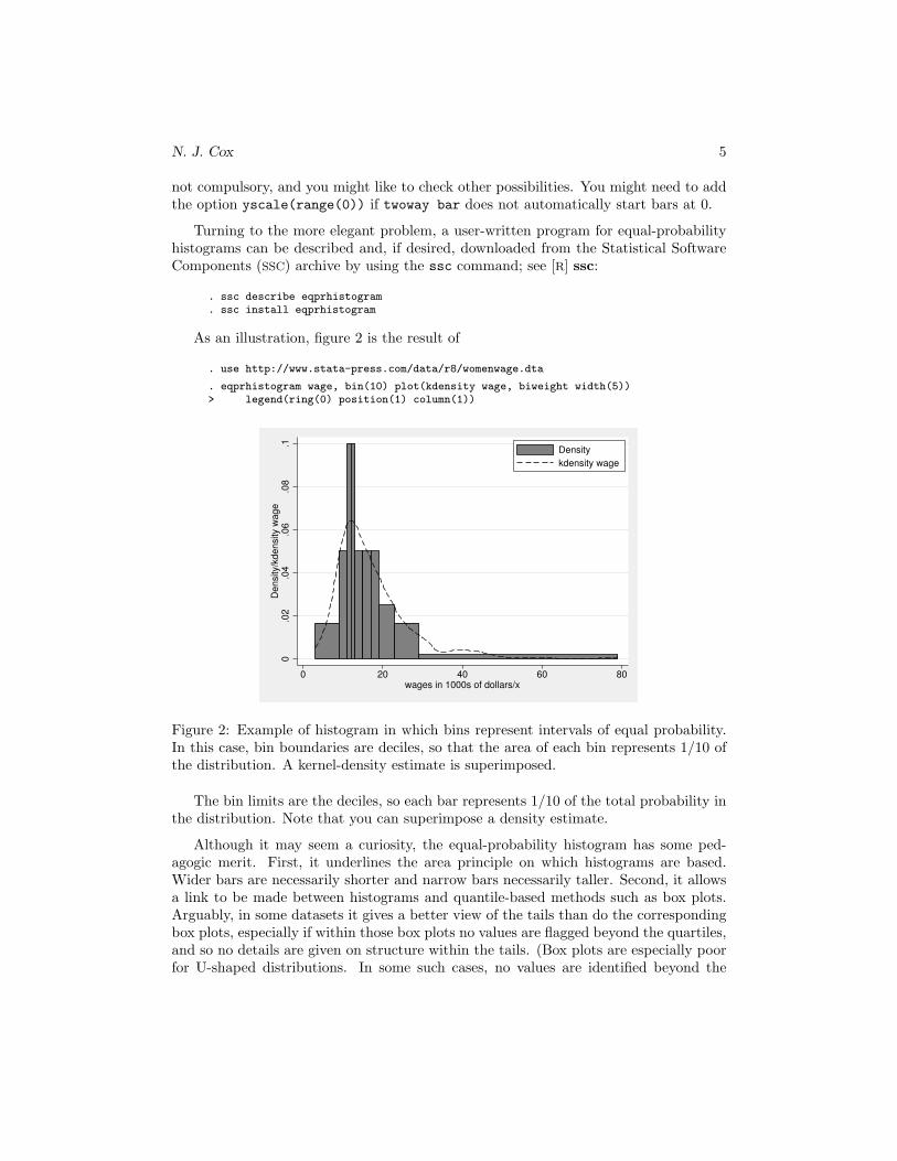
As an illustration, figure 2 is the result of

. use http://www.stata-press.com/data/r8/womenwage.dta

. eqprhistogram wage, bin(10) plot(kdensity wage, biweight width(5))> legend(ring(0) position(1) column(1))

0.0

2.0

4.0

6.0

8.1

Density/k

density w

age

0 20 40 60 80wages in 1000s of dollars/x

Density

kdensity wage

Figure 2: Example of histogram in which bins represent intervals of equal probability.In this case, bin boundaries are deciles, so that the area of each bin represents 1/10 ofthe distribution. A kernel-density estimate is superimposed.

The bin limits are the deciles, so each bar represents 1/10 of the total probability inthe distribution. Note that you can superimpose a density estimate.

Although it may seem a curiosity, the equal-probability histogram has some ped-agogic merit. First, it underlines the area principle on which histograms are based.Wider bars are necessarily shorter and narrow bars necessarily taller. Second, it allowsa link to be made between histograms and quantile-based methods such as box plots.Arguably, in some datasets it gives a better view of the tails than do the correspondingbox plots, especially if within those box plots no values are flagged beyond the quartiles,and so no details are given on structure within the tails. (Box plots are especially poorfor U-shaped distributions. In some such cases, no values are identified beyond the

6 Speaking Stata

quartiles, and the box plot reduces to a long box and two short tails. Even experiencedpeople can misread this as indicating a unimodal distribution, forgetting that if half thevalues lie inside the box, then, necessarily, half lie outside it.)

An equal-probability histogram is not suitable for all distributions. Given categor-ical, discrete, or highly rounded data, quantiles may be tied, especially if the num-ber of bins is large relative to the sample size. If the specified quantiles are tied,eqprhistogram refuses to draw the graph. A technical aside: whenever it does this,the exit code is 0. This is in part a diplomatic acknowledgment that inability to drawthe graph is either a feature of the data or a limitation of the method, rather than auser error. In addition, it implies that a loop through equal-probability histograms ofdifferent variables or groups will not fail merely because a particular graph is impossible.

2.3 Putting a rug underneath

One major merit of histograms is familiarity. All statistically minded people have lookedat many histograms, and nonstatistical people who use statistics have also usually comeacross them. Nevertheless, the basis of histograms, a division of a range into bins, isat best a means to an end, namely easy and effective visualization of a distribution,and at worst a serious distraction. Both psychologically and numerically, densities orfrequencies calculated from a set of bins can convey a poor idea of the detailed shapeof the distribution of a variable.

One simple way to enhance a histogram by forging a closer link with the raw data isto add a so-called rug, which as the name implies, is almost always placed underneaththe histogram. A rug is a very short, long display of point symbols, one for each distinctvalue. Often a vertical pipe symbol | is used to minimize overlap. Rugs may also beadded to other kinds of plots. There are many varied examples in Davison (2003).

Before version 8, Stata had graph options to combine rugs, which in Stata were calledoneway plots, with box plots and with scatterplots. These options are still accessibleunder graph7. However, they did not make the cut into the new graphics in that orsimilar form.

Although rugs are not explicitly provided in Stata 8, the procedure for weaving yourown rug is straightforward. Starting with a basic histogram for the same wage data,

. histogram wage, start(0) width(5)

we see that with these choices density varies up to about 0.07 per 1,000 dollars. Thatleads to a decision to put the rug at about −0.003 on that scale. We need a variable tohold this value:

. generate where = -0.003

N. J. Cox 7

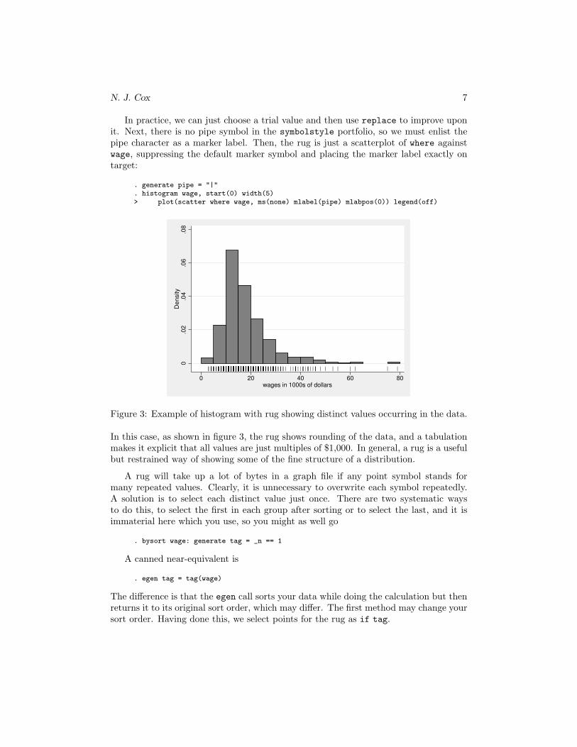
In practice, we can just choose a trial value and then use replace to improve uponit. Next, there is no pipe symbol in the symbolstyle portfolio, so we must enlist thepipe character as a marker label. Then, the rug is just a scatterplot of where againstwage, suppressing the default marker symbol and placing the marker label exactly ontarget:

. generate pipe = "|"

. histogram wage, start(0) width(5)> plot(scatter where wage, ms(none) mlabel(pipe) mlabpos(0)) legend(off)

||| ||| |||| |||| || |||||| || |||| || || |||| | ||||| | ||| ||||| | || || || || || ||| | |||||| || ||| ||| ||| | ||| ||||| ||| || | ||||| ||| ||||| || || | || || ||| |||| | | |||||| |||| || | ||||| || ||| |||||| | |||||| ||| |||| ||| | ||| |||| | ||||| ||| | ||||||| |||| || ||||| || ||||| ||| |||| || ||| | || || || ||| | ||| || || || || | || | |||| |||| || | ||||| ||||| || | || || ||| ||| || || || | ||| || ||| | |||| ||| || | ||| ||||| || || | ||| || || |||| || || | |||| ||| ||| || |||| | ||||| || || |||| ||| || || || ||| ||| || || ||| || ||| | ||| | ||| || |||| || | | ||| | ||| || |||| || || |||| || || | | || | || | | ||||| | | ||| || || || |||||| ||| || | ||| |||

0.0

2.0

4.0

6.0

8D

ensity

0 20 40 60 80wages in 1000s of dollars

Figure 3: Example of histogram with rug showing distinct values occurring in the data.

In this case, as shown in figure 3, the rug shows rounding of the data, and a tabulationmakes it explicit that all values are just multiples of $1,000. In general, a rug is a usefulbut restrained way of showing some of the fine structure of a distribution.

A rug will take up a lot of bytes in a graph file if any point symbol stands formany repeated values. Clearly, it is unnecessary to overwrite each symbol repeatedly.A solution is to select each distinct value just once. There are two systematic waysto do this, to select the first in each group after sorting or to select the last, and it isimmaterial here which you use, so you might as well go

. bysort wage: generate tag = _n == 1

A canned near-equivalent is

. egen tag = tag(wage)

The difference is that the egen call sorts your data while doing the calculation but thenreturns it to its original sort order, which may differ. The first method may change yoursort order. Having done this, we select points for the rug as if tag.

8 Speaking Stata

2.4 Horizontal histogram bars

The histogram display, by default, has the frequency axis vertical, as is conventional.The manual entry [G-2] graph combine shows how histograms may be placed verticallyand horizontally along the margins of a scatterplot. More generally, the horizontal

option may be used to reverse axes. This may sound merely cosmetic, but there areoccasions in which this layout appears more natural. In the environmental sciences,among other fields, height above and depth below some surface are key natural variables.The extra option yscale(reverse) would show depths the intuitive way up.

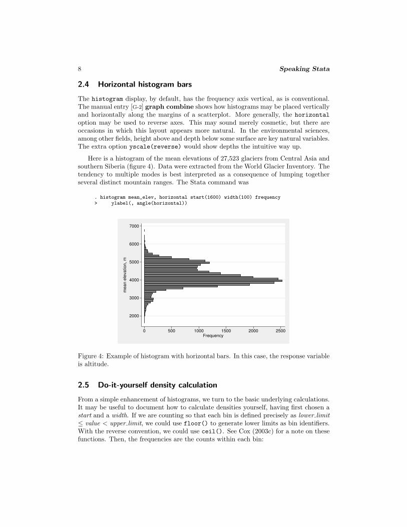
Here is a histogram of the mean elevations of 27,523 glaciers from Central Asia andsouthern Siberia (figure 4). Data were extracted from the World Glacier Inventory. Thetendency to multiple modes is best interpreted as a consequence of lumping togetherseveral distinct mountain ranges. The Stata command was

. histogram mean_elev, horizontal start(1600) width(100) frequency> ylabel(, angle(horizontal))

2000

3000

4000

5000

6000

7000

mean e

levation, m

0 500 1000 1500 2000 2500Frequency

Figure 4: Example of histogram with horizontal bars. In this case, the response variableis altitude.

2.5 Do-it-yourself density calculation

From a simple enhancement of histograms, we turn to the basic underlying calculations.It may be useful to document how to calculate densities yourself, having first chosen astart and a width. If we are counting so that each bin is defined precisely as lower limit

≤ value < upper limit, we could use floor() to generate lower limits as bin identifiers.With the reverse convention, we could use ceil(). See Cox (2003c) for a note on thesefunctions. Then, the frequencies are the counts within each bin:

N. J. Cox 9

. generate double lower = width * floor((varname - start) / width)

. bysort lower: generate frequency = _N

To get fractions and percents, we must be careful to count each value just once:

. by lower: generate double sum = frequency * (_n == 1)

. replace sum = sum(sum)

. generate fraction = frequency / sum[_N]

. generate percent = 100 * fraction

The density is then

. generate density = frequency / (width * _N)

Real calculations get messier once you build in selections if or in, subdivision intogroups defined by other variables, or missing values. The messy details are coded up inan egen function density() in the egenmore package on SSC.

3 Relatives of histogram: spikeplot, dotplot, and

onewayplot

One common reaction to histograms is to prefer more information in displaying distri-butions, especially in the tails. The optimistic view is that more details will turn outto be instructive fine structure. The corresponding pessimistic view is, naturally, thatsuch details will be best regarded as noise and, as such, an irreducible nuisance. Mostdiscussions stress the latter view over the former, but there can be real merit in playingdeterministic detective rather than stochastic skeptic.

The official commands spikeplot and dotplot and the user-written commandonewayplot offer different ways of showing more detail than do equivalent histograms.

spikeplot, by default, offers a spike for every distinct value—that is, no binning—and the opportunity to control binning by a round() option, which in effect controlsbin width. Historically, spikeplot offered, before Stata 8, the most obvious officialalternative to graph, histogram for getting a histogram-like display with more than50 bins. That role is now lost. However, its discrete representation of a frequencydistribution remains available for occasions when you want to emphasize the granularityof data, either as defined in principle (counted variables, in particular) or as measuredin practice. The display of the age distribution of Ghana given at [R] spikeplot is agood example of what spikeplot does best, revealing a fine structure of age preferences,including multiples of 5, even rather than odd ages, and so forth. There is some scope forcontrolling spike appearance if the default appearance (which is the default of twowayspike under the prevailing scheme) appears too exiguous.

dotplot, in contrast, is based on the idea (or the ideal) of showing a point symbol foreach value; exactly the same description covers rugs and onewayplot. Similar plots un-der a variety of names go back at least as far as van Langren (1644); see Tufte (1997, 15).Wilkinson (1999) gives several further references of historical interest. Chambers et al.

10 Speaking Stata

(1983) used the term one-dimensional scatterplots. The term oneway plots appears tohave been introduced by StataCorp in its earlier guise as Computing Resource Center(1985). Wild and Seber (2000) show many interesting examples of oneway plots.

dotplot, by default, offers, as far as possible, a point symbol for every value andsome binning. Binning can be controlled rather indirectly, although in practice, thedefault is usually adequate, and when desired, the binning can be switched off with thenogroup option. The main virtues of dotplots lie in their ability to show some featuresthat might otherwise be obscured by a series of touching bars, especially granularity anddetails of outliers or other extreme values in the tails. You can also show, for example,median and quartiles by horizontal marks and thus hybridize box plots and histograms.

The considerable flexibility of histogram, spikeplot, and dotplot might seem toleave few important gaps in their territory. Nevertheless, onewayplot was written toprovide some extra possibilities in this area; it also may be downloaded using ssc. Asmentioned earlier, graph, oneway did not survive as such into Stata 8, although theminor trickery needed to add rugs is just one illustration of how they can be emulatedfairly easily. onewayplot is essentially a convenience command that bundles togethervarious easy but tedious handles for making your own oneway plots. You can choosebetween horizontal and vertical layouts, while stack and center options produce a vari-ant on dotplot.1 There is, by default, no binning of data; binning may be accomplishedwith the width() option.

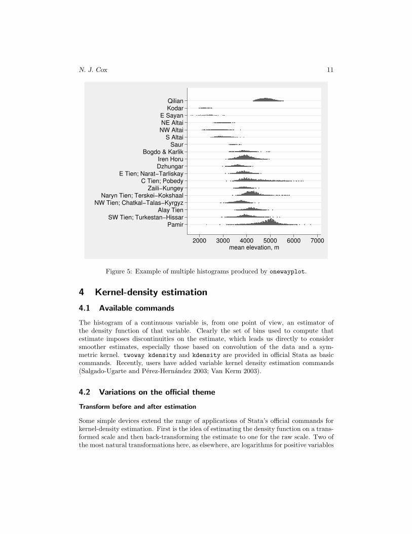
In figure 5, we show the results of a onewayplot using the handle of a regionalclassification to split the glacier elevations. Both histogram and dotplot strugglegiven 18 regions, some with fairly long names.

. onewayplot mean_elev, by(region) ytitle("") stack ms(oh) msize(tiny) width(20)

1. You can also type centre. An undocumented feature of dotplot is that centre is allowed as well ascenter. This is a convenience for speakers of languages, such as English, which use that spelling,and is emulated by onewayplot.

N. J. Cox 11

PamirSW Tien; Turkestan−Hissar

Alay TienNW Tien; Chatkal−Talas−Kyrgyz

Naryn Tien; Terskei−KokshaalZaili−Kungey

C Tien; PobedyE Tien; Narat−Tarliskay

DzhungarIren Horu

Bogdo & KarlikSaur

S AltaiNW AltaiNE AltaiE Sayan

KodarQilian

2000 3000 4000 5000 6000 7000mean elevation, m

Figure 5: Example of multiple histograms produced by onewayplot.

4 Kernel-density estimation

4.1 Available commands

The histogram of a continuous variable is, from one point of view, an estimator ofthe density function of that variable. Clearly the set of bins used to compute thatestimate imposes discontinuities on the estimate, which leads us directly to considersmoother estimates, especially those based on convolution of the data and a sym-metric kernel. twoway kdensity and kdensity are provided in official Stata as basiccommands. Recently, users have added variable kernel density estimation commands(Salgado-Ugarte and Perez-Hernandez 2003; Van Kerm 2003).

4.2 Variations on the official theme

Transform before and after estimation

Some simple devices extend the range of applications of Stata’s official commands forkernel-density estimation. First is the idea of estimating the density function on a trans-formed scale and then back-transforming the estimate to one for the raw scale. Two ofthe most natural transformations here, as elsewhere, are logarithms for positive variables

12 Speaking Stata

and logit-like transformations for proportions and other data measured on some interval(a, b). The underlying general principle is that, for a continuous monotone transforma-tion t(x), the densities f(x) and f{t(x)} are related by f(x) = f{t(x)}|dt/dx|. Thisprocedure is mentioned briefly by Silverman (1986, 27–30), although his worked exam-ple (page 28) is not very encouraging. Good expositions are given by Wand and Jones(1995, 43–45), Simonoff (1996, 61–64), and Bowman and Azzalini (1997, 14–16).

With a logarithmic transformation of x, we have

estimate of f(x) = estimate of f(log x)× (1/x)

given that d/dx(log x) = 1/x. Note in particular, if data are right skewed, that theresult of this transformation is more smoothing in the tail and less near the main partof the distribution than in the default method. I have found this to be one of themost valuable ways of going beyond the default. It fits very well both the commonfinding that positive variables are right-skewed, suggesting a transformation, such asthe logarithm, and the common attitude that results on the original scale are of directscientific or practical interest. To put it another way, the transformation behaves morelike a link function than a classical transformation, given that end results are on thescale of the original response. You can get the best of both worlds.

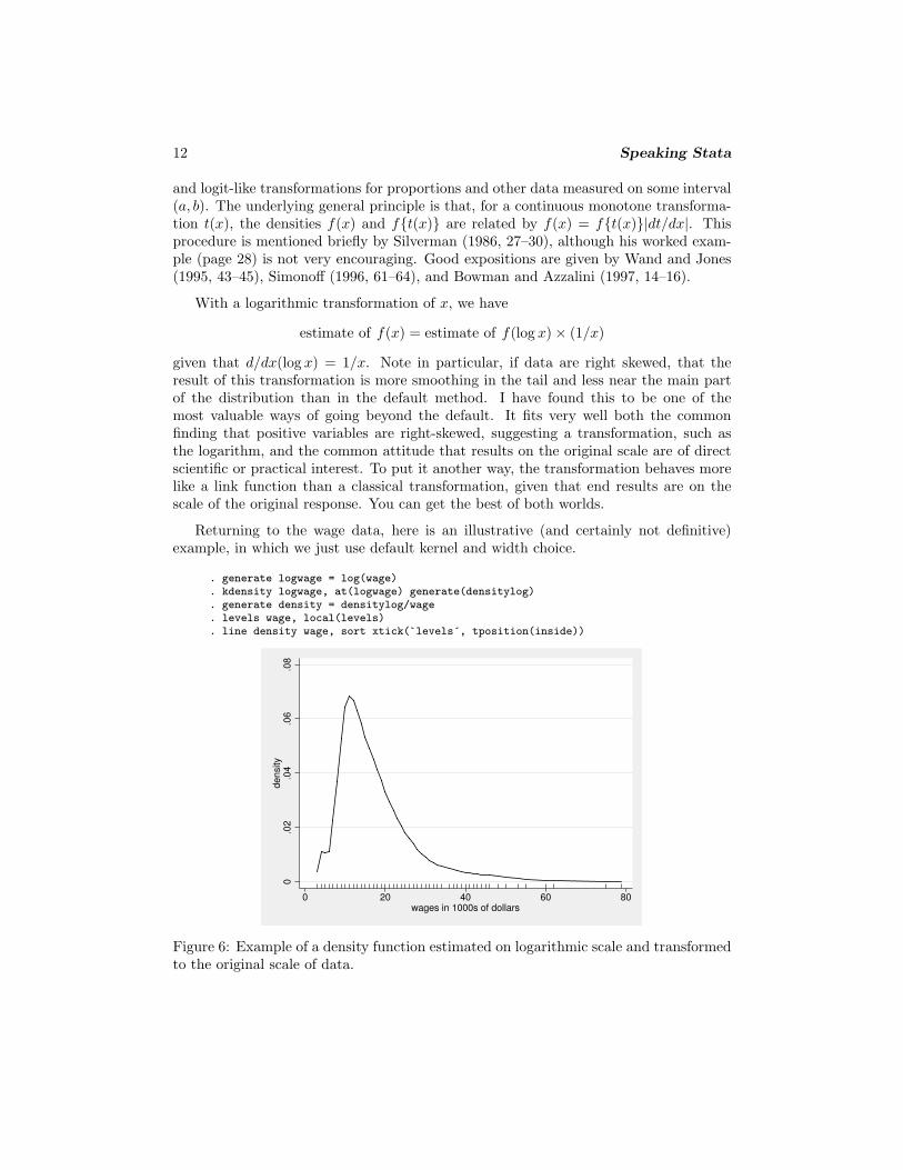
Returning to the wage data, here is an illustrative (and certainly not definitive)example, in which we just use default kernel and width choice.

. generate logwage = log(wage)

. kdensity logwage, at(logwage) generate(densitylog)

. generate density = densitylog/wage

. levels wage, local(levels)

. line density wage, sort xtick(`levels´, tposition(inside))

0.0

2.0

4.0

6.0

8density

0 20 40 60 80wages in 1000s of dollars

Figure 6: Example of a density function estimated on logarithmic scale and transformedto the original scale of data.

N. J. Cox 13

The density function, shown in figure 6, is much smoother in the tails than theequivalent default, which is not shown here. However, the step in the left-hand tail needsinvestigation: is this some odd artifact or a genuine feature of the data? Incidentally,another technique is used to show a rug by picking up a list of distinct values fromlevels (added to Stata on 16 April 2003). However, this technique is not as general asthat previously illustrated, as it hinges on the variable concerned having only integervalues. levels is not designed to work with noninteger numeric values.

Similarly with a logit-like transformation,

estimate of f(x) = {estimate of f(logit x)} (b− a)

(x− a)(b− x)

where logit x = log{(x− a)/(b− x)}, a slight generalization of the usual definition, forwhich a = 0, b = 1. Note that d/dx(logit x) = (b− a)/{(x− a)(b− x)}.

Density on a log scale

It can be natural to calculate f(log x) as a way of getting a better estimate of f(x). Itcan also be natural to calculate log{f(x)} as way of getting a better visualization off(x). This seems to be an old idea, periodically rediscovered. One venerable referenceis the work of the soldier, explorer, and scientist R. A. Bagnold (1937, 1941), whoworked on size distributions—especially those of sand—while at present the idea iswidely used in fields ranging from statistical physics (Bardou et al. 2002) to statisticalfinance (Hazelton 2003). There is clearly no barrier also to looking at log{f(log x)} orusing some other transformation before density estimation if it seems appropriate.

The highly original contribution of Bagnold deserves some explanation, as it appearsto be little known within the statistical sciences. Born in England in 18962, he joinedthe British army from school and served in the First World War. He then took anengineering degree at Cambridge. Remaining in the army, he used leaves to travel andexplore, particularly on pioneering long trips into the deserts of Egypt, Sudan, andLibya using specially adapted cars. This provoked an interest in the physics of blownsand, leading ultimately to a now-classic monograph (Bagnold 1941). Wind transportof loose particles is highly size selective, as ordinary experience confirms: very coarsematerial will not move, while very fine material may easily be lofted high into theatmosphere and carried over vast distances. Thus, the particle size distribution of adeposit (say from a sand dune) is of central interest. Bagnold found plots of log densityversus log grain diameter the most helpful way to show his data. It seems clear from hisvery readable autobiography (1990), published just after his death, that the crucial firststep of plotting densities on a log scale owed most to an engineer’s feeling of a sensiblething to do. By thinking for himself, he was not inhibited by ideas on what was orwas not standard statistical practice. Much later, Bagnold returned to the question andcontributed to the development of log-hyperbolic distributions by Ole Barndorff-Nielsen.There is a full bibliography of his publications in Thorne et al. (1988).

2. His sister was Enid Bagnold, later a novelist, dramatist, and poet, and best remembered for thechildren’s classic National Velvet.

14 Speaking Stata

Several properties are simple on a log-density scale. One exploited by Bagnold isthat a normal (Gaussian) density plots as a parabola

log f(x) = − log(σ√2π

)− (x− µ)

2

2σ2

while exact or approximate exponential or power-law decay of density will show exact orapproximate linear patterns, the latter requiring also a logarithmic scale for the variable.

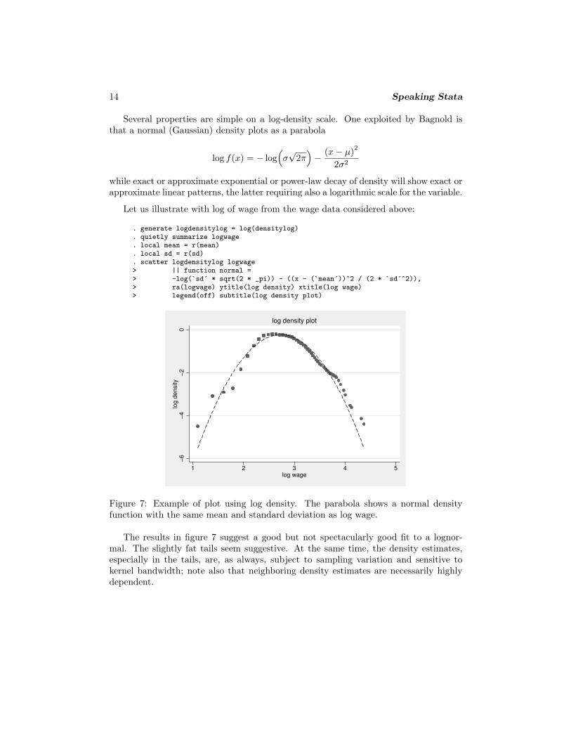
Let us illustrate with log of wage from the wage data considered above:

. generate logdensitylog = log(densitylog)

. quietly summarize logwage

. local mean = r(mean)

. local sd = r(sd)

. scatter logdensitylog logwage> || function normal => -log(`sd´ * sqrt(2 * _pi)) - ((x - (`mean´))^2 / (2 * `sd´^2)),> ra(logwage) ytitle(log density) xtitle(log wage)> legend(off) subtitle(log density plot)

−6

−4

−2

0lo

g d

ensity

1 2 3 4 5log wage

log density plot

Figure 7: Example of plot using log density. The parabola shows a normal densityfunction with the same mean and standard deviation as log wage.

The results in figure 7 suggest a good but not spectacularly good fit to a lognor-mal. The slightly fat tails seem suggestive. At the same time, the density estimates,especially in the tails, are, as always, subject to sampling variation and sensitive tokernel bandwidth; note also that neighboring density estimates are necessarily highlydependent.

N. J. Cox 15

What is implemented above is just a first stab. Hazelton (2003) suggests variousrefinements, including robust estimation of the mean and standard deviation and, givena density estimation bandwidth h, fitting a normal with variance sd2 + h2 to correctfor side-effects of using a kernel.

Density on a root scale

There would also be some advantages to a square-root scale, given that densities behavea bit like counts, for which a root transformation is often the first to be tried. Also, thesquare root of a Gaussian shape is another Gaussian shape. So we can have our cakeand eat it too: hunt for a Gaussian yet benefit from stabilized sampling fluctuation.Check the assertion with

. twoway function sqrt(normden(x)), range(-4 4)

There is a root option in spikeplot for a similar reason. Tukey (1977, chapter 17)worked through a bundle of related ideas, which seem to have been little explored since.

Intensities, too

Those interested in data on events, considered as the result of a point process in onedimension (most obviously, time or space), should note that Stata’s kernel-density com-mands can readily be used to estimate the intensity function (say, frequency per unitof time or space). Suppose that a variable contains dates of earthquakes, eruptions,strikes, honors for a sports team, or whatever else is of interest. To get results on anintensity scale, just multiply ‘density’ by the number of observed data points. A keydetail is that intensities will be smoothed beyond the beginning and the end of theinterval in question; whether this is tolerable or further surgery is desired is a questionfor the user.

5 Quantile plots and distribution plots

Another key approach eschews any kind of binning or smoothing and starts with theidea of directly showing the pattern of the quantiles (the ordered values). Formally,we order n data values for a variable x and label them such that x(1) ≤ · · · ≤ x(n).quantile has long been available as an official Stata command for quantile plots, inwhich the x(i) are plotted against (i − 0.5)/n. See [R] diagnostic plots. The termquantile plot appears in Chambers et al. (1983) and Cleveland (1993, 1994). Modernuse of quantile plots and their relatives stems largely from the path-breaking paper ofWilk and Gnanadesikan (1968). Examples of antecedents from the nineteenth centurycan be found in Quetelet (1827) and Galton (1875); see Stigler (1986, 167, 270).

Essentially the same information can be shown in a plot of cumulative distributionfunctions or of survival (a.k.a., survivor, reliability, complementary, or reverse distribu-tion) functions, in which we plot either probabilities or frequencies of values being ≤ x

16 Speaking Stata

or > x. In many biomedical or engineering applications, the survival function appearscloser to the practical problem, the name being suitably evocative if data are indeedtimes to patient death, component failure, or something similar.

According to Hald (1990, 108), the first graph of (the complement of) a distributionfunction appears in a 1669 letter from Christiaan Huygens (1629–1695) to his brotherLodewijk (1631–1699). He plotted a survival function from data from the life tableof John Graunt (1620–1674). Huygens made numerous contributions to mathematics,astronomy, and physics, studying, among many other matters, games of chance, thecollision of elastic bodies, the rings of Saturn, the pendulum clock, and the wave theoryof light.

In Stata 8, the graphics of quantile were revised to match the new graphics, butthe functionality was unchanged. A broader command is qplot (Cox 2004), which inmost respects is a generalization of quantile; just one detail is omitted, the referenceline. It supersedes the previous program quantil2 (Cox 1999b, 2001).

Stata already has an official graph command for survival functions, sts graph. Ifyour data really are survival times and you have any of the complications that are thestuff of survival analysis, such as censoring or subjects entering at different times, youshould use sts graph. However, it is not and does not purport to be a general purposecommand for all kinds of distribution.

In addition, the official command cumul ([R] cumul) is available to calculate thecumulative distribution function for a single variable, after which the function may beplotted using twoway. The user with several variables to be compared or with an interestin survival functions thus needs to repeat the cumul command or take the further stepof calculating survival functions from cumulative distribution functions. A commanddistplot that bundles calculation and graphing steps together is, however, available(Cox 1999a, 2003a,b).

qplot and distplot are, in effect, siblings. The choice between them is most obvi-ously one of choice of axes and thus, in a sense, trivial, but different conventions mayseem natural for different problems and even different fields or traditions. In particular,there seems to be a growth of interest in quantile functions as responses, which makesqplot a possible choice (see, for example, Gilchrist 2000).

qplot and distplot have in common

1. Support for graphing several variables.

2. Support for graphing several groups, through a by() option.

3. Choice of twoway plottypes, from area, bar, connected, dot, dropline, line,scatter, or spike. These are not in general equally useful or attractive, but thereis at least much choice, courtesy of twoway’s generous design.

4. Support for reversing the sort order so that values decrease from top left.

5. Support for alternative transformed scales.

N. J. Cox 17

In addition, qplot has support for choice of a in a general rule for plotting position(i − a)/(n − 2a + 1) for i = 1, . . . , n. The default is a = 0.5, giving (i − 0.5)/n. Otherchoices include a = 0, giving i/(n + 1), and a = 1/3, giving (i − 1/3)/(n + 1/3). Thechoice is often immaterial, but some authorities have strong opinions on the best choiceon various grounds, some even statistical. For more discussion and references, see Cox(1999b).

6 Skewness plots

The skewness of a variable is often of interest, perhaps especially as an indicator ofpotential problems in subsequent analysis. Commonly a single measure is used, whetherthe moment-based measure produced by summarize, detail or other measures (which,in most cases, are readily calculated from the output of summarize). Graphically,skewness may be assessed with varying degrees of ease and efficiency from the plotsmentioned so far, but there is also a case for a customized design.

Various possibilities are based on the quantiles (Gnanadesikan 1977, 1997). Thequantiles may be paired as lower and upper quantiles x(1) and x(n), x(2) and x(n−1),etc., and a median may be calculated in the usual way.

Stata supports symplot, a plot of (upper quantile − median) versus (median − lowerquantile), for which the reference situation of symmetry or lack of skew plots as a line ofequality. See [R] diagnostic plots. However, symplot will show only a single group ofdata and thus cannot be used for comparisons, while a plot with a sloping reference lineis more difficult to deal with than the plot now to be described, which has horizontalreference lines.

skewplot produces, by default, a plot of the midsummary versus the spread for thevariables supplied, also known as the mid-versus-spread plot. With the skew option,it produces a plot of the skewness function versus the spread function. Such plotsconvey both the general character and the fine structure of the symmetry or skewness ofdatasets and can be used to compare distributions or to assess whether transformationsare necessary or effective.

There are some little-used terms here, so we need a few definitions. In a perfectlysymmetric set of data, the midsummaries (x(1) + x(n))/2, (x(2) + x(n−1))/2, etc., wouldall be identical and equal to the median. A plot of each midsummary (or mean of lowerand upper quantiles) (x(i) + x(n−i+1))/2 versus each difference or spread of lower andupper quantiles x(n−i+1)−x(i) would, thus, yield a horizontal straight line. Conversely,skewness in sets of data will be reflected by departures from horizontality. In particular,right skewness would be shown by rising lines and left skewness by falling lines.

Apart from the divisor of 2, this plot was suggested by J. W. Tukey (Wilk andGnanadesikan 1968). See also Gnanadesikan (1977, 1997, chapter 6.2) or Fisher (1983).The form used here and the name mid-versus-spread plot are found in Hoaglin (1985).It is usual to plot only that half of the sample results for which spread is ≥ 0.

18 Speaking Stata

The skew option produces an alternative form promoted by Benjamini and Krieger(1996, 1999). Consider the identity, which introduces their terminology,

x(n−i+1) = median + (x(n−i+1) − x(i))/2 + (x(i) + x(n−i+1) − 2×median)/2

= median + spread function + skewness function

for x(i) in the lower half of a sample. This leads to a plot of the skewness functionversus the spread function, known as the skewness versus spread plot. Note that theskewness function is (midsummary − median) and so will be constant and zero for aperfectly symmetric distribution and that the spread function is half the spread of themid versus spread plot. In short, the skew option does not change the configuration ofthe plot but merely the labeling of the axes.

In addition, the ratio of the skewness and spread functions or

x(i) + x(n−i+1) − 2×median

x(n−i+1) − x(i)

is a measure of skewness (in the traditional sense) originally suggested for quartiles byBowley (1902) and generalized to this form by David and Johnson (1956). Anotherincarnation is as the p-skewness index (Gilchrist 2000, 54, 72).3 It varies between −1and 1. A similar general measure was used by Parzen (1979). Graphically this measureis the slope of the line connecting (0, 0) and each data point if the skew option is used.

See Benjamini and Krieger (1996, 1999) and Groeneveld (1998) for concise reviewstracing such ideas from late 19th-century antecedents to recent work and further detailson the interpretation of the skewness-versus-spread plot.

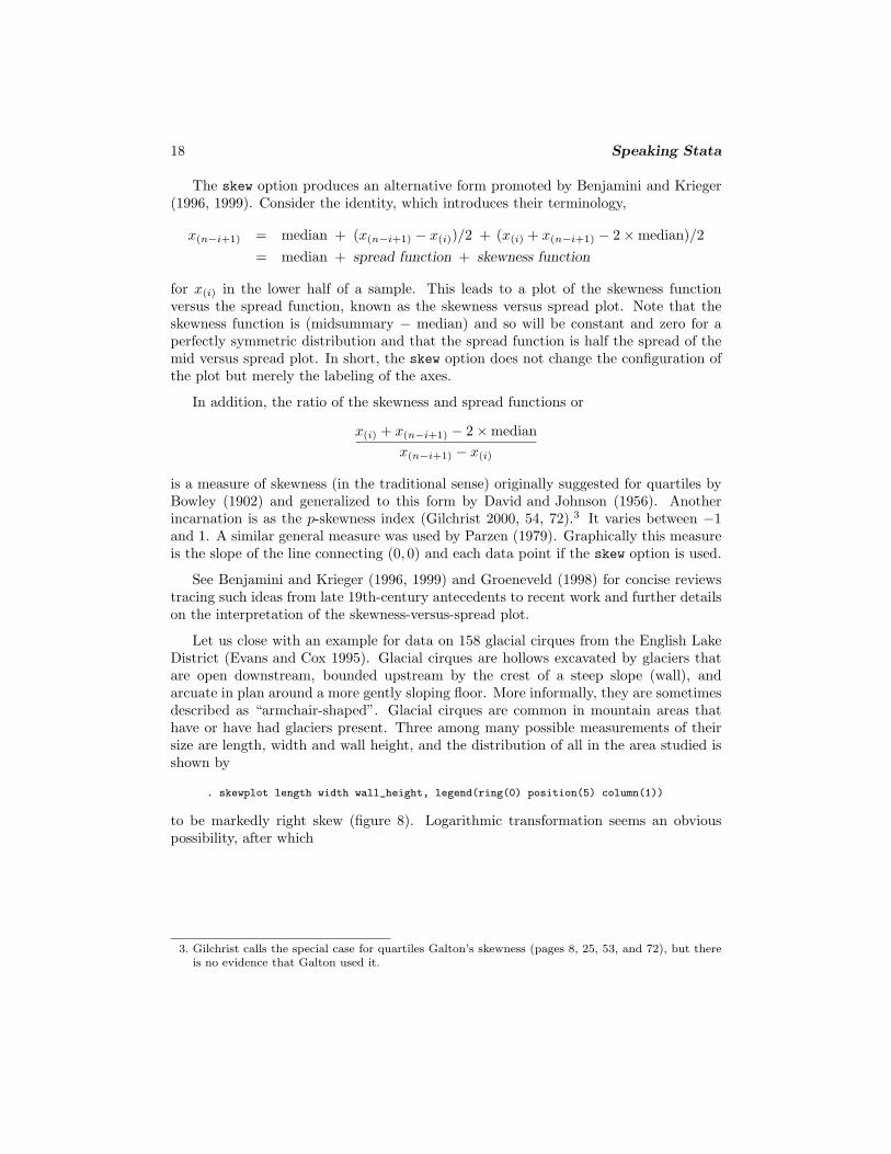
Let us close with an example for data on 158 glacial cirques from the English LakeDistrict (Evans and Cox 1995). Glacial cirques are hollows excavated by glaciers thatare open downstream, bounded upstream by the crest of a steep slope (wall), andarcuate in plan around a more gently sloping floor. More informally, they are sometimesdescribed as “armchair-shaped”. Glacial cirques are common in mountain areas thathave or have had glaciers present. Three among many possible measurements of theirsize are length, width and wall height, and the distribution of all in the area studied isshown by

. skewplot length width wall_height, legend(ring(0) position(5) column(1))

to be markedly right skew (figure 8). Logarithmic transformation seems an obviouspossibility, after which

3. Gilchrist calls the special case for quartiles Galton’s skewness (pages 8, 25, 53, and 72), but thereis no evidence that Galton used it.

N. J. Cox 19

200

400

600

800

1000

Mid

sum

mary

0 500 1000 1500Spread

length, m

width, m

wall height, m

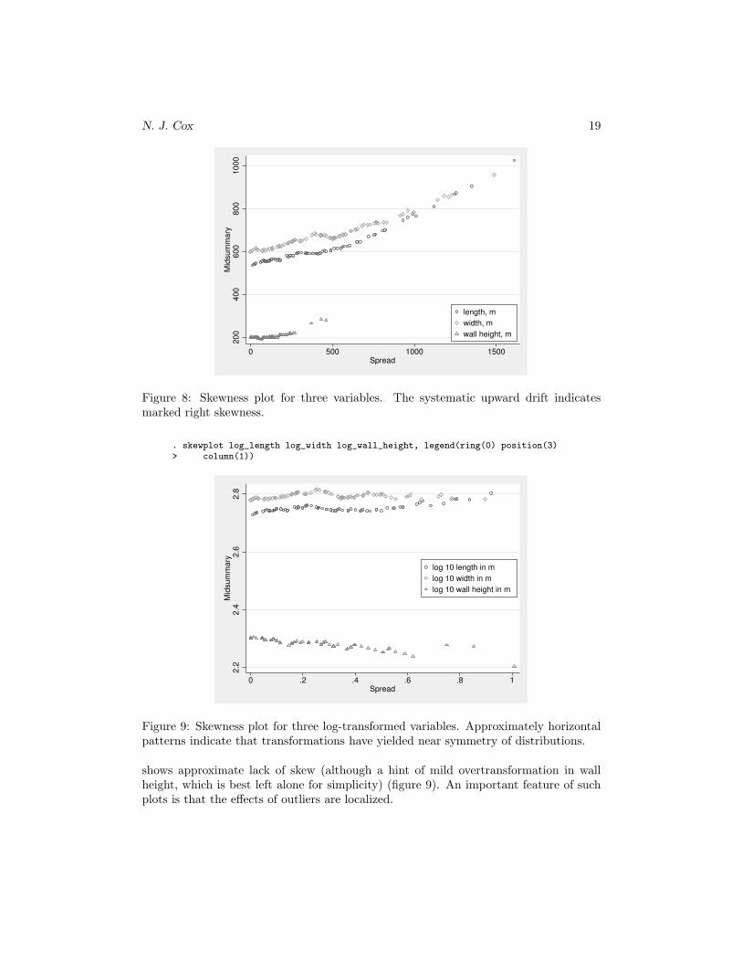
Figure 8: Skewness plot for three variables. The systematic upward drift indicatesmarked right skewness.

. skewplot log_length log_width log_wall_height, legend(ring(0) position(3)> column(1))

2.2

2.4

2.6

2.8

Mid

sum

mary

0 .2 .4 .6 .8 1Spread

log 10 length in m

log 10 width in m

log 10 wall height in m

Figure 9: Skewness plot for three log-transformed variables. Approximately horizontalpatterns indicate that transformations have yielded near symmetry of distributions.

shows approximate lack of skew (although a hint of mild overtransformation in wallheight, which is best left alone for simplicity) (figure 9). An important feature of suchplots is that the effects of outliers are localized.

20 Speaking Stata

7 Conclusions

With one command or another, users can now plot univariate distributions in manydifferent ways. You can choose between several depictions of the density function orseveral depictions of the distribution function or its inverse, the quantile function. Youcan choose discrete or continuous representations and vertical or horizontal alignments.Less obviously, it is straightforward to add details (for example, rugs of distinct datavalues) or exploit the inbuilt flexibility of graph (for example, by looking at densityestimates on a log scale or by constructing your own histogram with varying bin width).

The theme of distributions will continue into the next column but with a focus oncategorical data. Distributions of categorical variables may be shown in a variety ofdisplays: the survey will range from old staples to less well-known plots, with emphasison the important special cases of graded data and of three variables with constant sum.

8 Acknowledgments

Ian Evans provided the Lake District cirques data, pointed me to the World GlacierInventory data, and participated in many discussions on statistical graphics over morethan 30 years. Marcello Pagano persistently urged the merits of equal-probability his-tograms and parenthetically underlined the connection with chi-squared tests. VinceWiggins specifically alerted me to spanning bars and generally advised on strategies andtactics for using the new graphics. Elizabeth Allred, Ronan Conroy, Philip Ender, andRoger Harbord made helpful comments during development of various predecessors orversions of some programs discussed here. Richard Groeneveld kindly tracked down theBowley reference.

9 References

Altman, D. G. 1991. Practical Statistics for Medical Research. London: Chapman &Hall.

Bagnold, R. A. 1937. The size-grading of sand by wind. Proceedings of the RoyalSociety, Series A 163: 250–264.

———. 1941. The Physics of Blown Sand and Desert Dunes. London: Methuen.

———. 1990. Sand, Wind, and War: Memoirs of a Desert Explorer. Tucson: Universityof Arizona Press.

Bardou, F., J.-P. Bouchaud, A. Aspect, and C. Cohen-Tannoudji. 2002. Levy Statisticsand Laser Cooling: How Rare Events Bring Atoms to Rest. Cambridge: CambridgeUniversity Press.

Benjamini, Y., and A. M. Krieger. 1996. Concepts and measures for skewness withdata-analytic implications. Canadian Journal of Statistics 24: 131–140.

N. J. Cox 21

———. 1999. Skewness—concepts and measures. In Encyclopedia of Statistical SciencesUpdate, ed. S. Kotz, C. B. Read, and D. L. Banks, vol. 3, 663–670. New York: Wiley.

Bowley, A. L. 1902. Elements of Statistics. 2nd ed. London: P. S. King.

Bowman, A. W., and A. Azzalini. 1997. Applied Smoothing Techniques for Data Anal-ysis: The Kernel Approach with S-Plus Applications. Oxford: Oxford UniversityPress.

Breiman, L. 1973. Statistics: With a View Toward Applications. Boston: HoughtonMifflin.

Chambers, J. M., W. S. Cleveland, B. Kleiner, and P. A. Tukey. 1983. GraphicalMethods for Data Analysis. Belmont, CA: Wadsworth.

Cleveland, W. S. 1993. Visualizing Data. Summit, NJ: Hobart.

———. 1994. The Elements of Graphing Data. Rev. ed. Summit, NJ: Hobart.

Computing Resource Center. 1985. STATA/Graphics User’s Guide. Los Angeles, CA:Computing Resource Center.

Cox, N. J. 1999a. gr41: Distribution function plots. Stata Technical Bulletin 51: 12–16.Reprinted in Stata Technical Bulletin Reprints, vol. 9, pp. 108–112. College Station,TX: Stata Press.

———. 1999b. gr42: Quantile plots, generalized. Stata Technical Bulletin 51: 16–18.Reprinted in Stata Technical Bulletin Reprints, vol. 9, pp. 113–116. College Station,TX: Stata Press.

———. 2001. gr42.1: Quantile plots, generalized: update to Stata 7.0. Stata TechnicalBulletin 61: 10–11. Reprinted in Stata Technical Bulletin Reprints, vol. 10, pp. 55–56.College Station, TX: Stata Press.

———. 2003a. Software update: gr41 1: Distribution function plots. Stata Journal 3:211.

———. 2003b. Software update: gr41 2: Distribution function plots. Stata Journal 3:449.

———. 2003c. Stata tip 2: Building with floors and ceilings. Stata Journal 3: 446–447.

———. 2004. Software update: gr42 2: Quantile plots, generalized. Stata Journal 4:97.

David, F. N., and N. L. Johnson. 1956. Some tests of significance with ordered variables.Journal of the Royal Statistical Society, Series B 18: 1–20.

Davison, A. C. 2003. Statistical Models. Cambridge: Cambridge University Press.

Evans, I. S., and N. J. Cox. 1995. The form of glacial cirques in the English LakeDistrict, Cumbria. Zeitschrift fur Geomorphologie 39: 175–202.

22 Speaking Stata

Fisher, N. I. 1983. Graphical methods in nonparametric statistics: A review and anno-tated bibliography. International Statistical Review 51: 25–38.

Freedman, D., R. Pisani, and R. Purves. 1978. Statistics. New York: W. W. Norton.

Galton, F. 1875. Statistics by intercomparison, with remarks on the law of frequencyof error. Philosophical Magazine, 4th ser., 49: 33–46.

Gilchrist, W. G. 2000. Statistical Modelling with Quantile Functions. Boca Raton, FL:Chapman & Hall/CRC.

Gnanadesikan, R. 1977. Methods for Statistical Data Analysis of Multivariate Obser-vations. New York: Wiley.

———. 1997. Methods for Statistical Data Analysis of Multivariate Observations. 2nded. New York: Wiley.

Groeneveld, R. 1998. Skewness, Bowley’s measure of. In Encyclopedia of StatisticalScienes Update, ed. S. Kotz, C. B. Read, and D. L. Banks, vol. 2, 619–621. NewYork: Wiley.

Gumbel, E. J. 1943. On the reliability of the classical chi-square test. Annals of Math-ematical Statistics 14: 253–263.

Hald, A. 1990. A History of Probability and Statistics and their Applications before1750. New York: Wiley.

Hazelton, M. L. 2003. A graphical tool for assessing normality. American Statistician57: 285–288.

Hoaglin, D. C. 1985. Using quantiles to study shape. In Exploring Data Tables, Trends,and Shapes, ed. D. C. Hoaglin, F. Mosteller, and J. W. Tukey, 417–460. New York:Wiley.

van Langren, M. F. 1644. La Verdadera Longitud po Mar y Tierra. Antwerp.

Mann, H. B., and A. Wald. 1942. On the choice of the number of class intervals in theapplication of the chi-square test. Annals of Mathematical Statistics 13: 306–317.

Parzen, E. 1979. Nonparametric statistical data modeling. Journal of the AmericanStatistical Association 74: 105–131.

Quetelet, A. 1827. Recherches sur la population, les naissances, les deces, les prisons,les depots de mendicite, etc., dans le Royaume des Pays-Bas. Nouveaux Memoires del’Academie Royale des Sciences et Belles-lettres de Bruxelles 4: 117–192.

Salgado-Ugarte, I. H., and M. A. Perez-Hernandez. 2003. Exploring the use of variablebandwidth kernel density estimators. Stata Journal 3: 133–147.

Scott, D. W. 1992. Multivariate Density Estimation: Theory, Practice, and Visualiza-tion. New York: Wiley.

N. J. Cox 23

Silverman, B. W. 1986. Density Estimation for Statistics and Data Analysis. BocaRaton, FL: Chapman & Hall/CRC.

Simonoff, J. S. 1996. Smoothing Methods in Statistics. New York: Springer.

Stigler, S. M. 1986. The History of Statistics: The Measurement of Uncertainty before1900. Cambridge, MA: Belknap Press.

Thorne, C. R., R. C. MacArthur, and J. B. Bradley, eds. 1988. The Physics of SedimentTransport by Wind and Water: A Collection of Hallmark Papers by R. A. Bagnold.New York: American Society of Civil Engineers.

Tufte, E. R. 1997. Visual Explanations: Images and Quantities, Evidence and Narrative.Cheshire, CT: Graphics Press.

Tukey, J. W. 1977. Exploratory Data Analysis. Reading, MA: Addison–Wesley.

Van Kerm, P. 2003. Adaptive kernel density estimation. Stata Journal 3: 148–156.

Wand, M. P., and M. C. Jones. 1995. Kernel Smoothing. London: Chapman &Hall/CRC.

Wild, C. J., and G. A. F. Seber. 2000. Chance Encounters: A First Course in DataAnalysis and Inference. New York: Wiley.

Wilk, M. B., and R. Gnanadesikan. 1968. Probability plotting methods for the analysisof data. Biometrika 55: 1–17.

Wilkinson, L. 1999. Dot plots. American Statistician 53: 276–281.

About the author

Nicholas Cox is a statistically minded geographer at the University of Durham. He contributestalks, postings, FAQs, and programs to the Stata user community. He has also co-authoredfourteen commands in official Stata. He was an author of several inserts in the Stata Technical

Bulletin and is Executive Editor of the Stata Journal.