The Riemann Hypothesis

C. Calderon

Departamento de Matematicas. Facultad de Ciencia y Tecnologıa

Universidad del Paıs Vasco. 48080 Bilbao, Spain

mtpcagac@lg.ehu.es

Monografıas de la Real Academia de Ciencias de Zaragoza. 26: 1–30, (2004).

Abstract

Riemann proved (see [53], [37] and preferably Edwards’ book [15]), that ζ(s)

has an analytic continuation to the whole plane apart from a simple pole at s = 1.

Moreover, he showed that ζ(s) satisfies the functional equation

π−s/2Γ(s/2)ζ(s) = π−(1−s)/2Γ((1 − s)/2)ζ(1 − s).

Riemann uses the functional equation to deduce an approximate formula for π(x) =

#p ≤ x; p prime: that is

π(x) ∼ Li(x) +N∑

n=2

µ(n)n

Li(x1n ), N > log x/ log 2.

In the paper (see [53]), he stated also that ζ(s) had infinitely many non trivial roots

and that it seemed probable that they all have real part 1/2.

1 Distribution of prime numbers

Among the positive integers there is a sub-class of special importance, that is, the class of

primes. Some questions about primes are: a) How many prime numbers are there? and

b) How are the prime numbers distributed?

The answer to the question of how many prime numbers are there is given by the

theorem of Euclid (Elements, Book 9, Prop. 20): There exist infinitely many prime

numbers. In the proof of Euclid, to prove the theorem, it will suffice to prove that if

p1, p2, · · · , pn is any finite set of primes, then we can find a prime number that is not in

the set.

As usual Z will denote the ring of integers, Q the field of rational numbers, R the field

of real numbers and C the field of complex numbers. Also we shall denote by N the set

of positive (natural) integers, not including 0.

1

In 1737, Euler proved the existence of an infinity of primes by a new method, which

shows moreover that the series∑

pnp−1

n is divergent. Euler’s work is based on the idea of

using an identity in which the primes appear on one side but not on the other. Stated

formally his identity is

∏p

1 − p−s−1 =∞∑

n=1

n−s, (s > 1) (1)

where p ranges over all prime numbers. This formula results from expanding each of the

factors on the left

(1 − x)−1 = 1 + x + x2 + . . . , x = p−s.

As their product is a sum of terms of the form (pα11 · · · pαr

r )−s, where p1 = p2 = · · · = pr,

the formula (1) is deduced by using the fundamental theorem of arithmetic: Each natural

number n > 1 can be decomposed uniquely, up to order of the factors, as a product of

prime numbers.

From an old theorem of Nicole Oresme (1360), we have that: The harmonic series∑∞n=1 1/n = ζ(1) is divergent.

Function π(x). We introduce a function π(x) which has become universally accepted

and means the number of primes not exceeding x. If p1 = 2, p2 = 3, · · · , and pn denote

the nth prime number, then for each integer n we have π(pn) = n. It follows from Euclid′s

theorem that π(x) → ∞ as x → ∞.

Legendre. Experimentally, Legendre conjectured in 1798 and again in 1808 the hypoth-

esis that

π(x) ∼ x

log x − A(x), lim

x→∞A(x) = 1, 08366 . . .

Gauss. Gauss [20], in a letter to the astronomer Enke in 1849, stated that he had found

in his early years (at age 17, in 1792), that the number π(x) of primes up to x and the

integral ∫ x

2

dt

log t

are asymptotically equal. However, Gauss does not mention Euler’s formula and he gives

no analytic basis for the approximation, which he presents only on the basis of extensive

computations. So, Gauss conjectured that

π(x) ∼ x

log x, x → ∞

This conjecture, now a theorem, is called the “Prime Number Theorem”.

Chebyshev. The first serious work on the function π(x) is due to the Russian mathemati-

cian Chebyshev. On May 24, 1848, Chebyshev read at the Academy of St. Petersburg his

2

first memoir on the distribution on prime numbers, later published in 1850. He proved,

using elementary methods, that for every ε > 0 there exists x0 > 0 such that if x > x0,

then

(C ′ − ε)x

log x< π(x) < (C + ε)

x

log x

where C ′ = 21/231/351/530−1/30 < 1, C = (6/5)C ′. Moreover, Chebyshev showed that if

the limit

limx→∞

π(x)

x/ log x

exists, it must be equal to 1. He deduced also, that Legendre’s approximation of π(x)

cannot be true, unless 1, 08366 is replaced by 1.

Dirichlet. In 1837, Dirichlet proved his famous theorem of the existence of infinitely

many primes in any arithmetic progression n ≡ h (mod k), with h and k positive co-

primes integers. The main novelty in his proof consisted in making use of characters mod-

ulo k, that is, homomorphisms from the group (Z/kZ)∗ of invertible residues (mod k)

into the multiplicative group of complex numbers of modulus 1, (see Tenenbaum [59] cap

II.8, for all these facts).

Riemann. Riemann considers the zeta-function defined by the generalized harmonic

series ζ(s) =∑

n−s, where the letter s denotes a complex variable s = σ + it σ > 1

its real part and t its imaginary part. If σ > 1 we can represent ζ(s) by an absolutely

convergent infinite product, namely

ζ(s) =∏

p

1 − p−s−1. (2)

The Riemann hypothesis appears in a paper over the number of primes less than a

given magnitude, published in 1859 by Riemann (see-preferably- Edwards’ book [15], also

[53], or [37]). It is the only work that Riemann published in number theory, but most of

Riemann’s ideas have been incorporated in later to the work of many mathematicians.

In 1859 Dirichlet died and Riemann was appointed to the chair of mathematics at

Gottingen. A few days later Riemann was elected to the Berlin Academy of Sciences. He

had been proposed by Kummer, Borchardt and Weierstrass. Riemann, newly elected to

the Berlin Academy of Sciences had to report on their most recent research and he sent

a report on Uber die Anzahl der Prinzahlen unter einer gegebener Grose. Riemann style

is extremely difficult, his paper is extremely condensed and in particular [53], is probably

a summary of very extensive researches which he never found the time to expound at

grater length. The main purpose of the paper was to give estimates for the number of

primes less than a given number. In this paper he stated that ζ(s) had infinitely many

non trivial roots and that it seemed probable that they all have real part 1/2. Many of

3

the results which Riemann obtained in this paper were later proved by Hadamard, de la

Vallee-Poussin, Hardy and von Mangoldt.

2 Analytic continuation

The development of complex analysis was a central preoccupation of Riemann’s and so it

comes as no surprise that from the beginning Riemann considered the zeta-function as an

analytic function. He first showed that ζ(s) had an analytic continuation to the complex

plane as a meromorphic function which has only one singularity, a simple pole of residue

1 at s = 1.

Riemann derives his functional equation for ζ(s) from the representation of the gamma-

function as an integral, for which Riemann still used the symbol Π

Γ(s) = Π(s − 1) =

∫ ∞

0

e−uus−1du. (3)

The gamma-function defined by (3) has meromorphic continuation to all of C, and is

analytic except at s = 0,−1,−2, · · · ,−n, · · ·, where it has simple poles.

If n is a positive integer, we have, on writing nx for u

Γ(s)

ns=

∫ ∞

0

e−nxxs−1dx.

Hence

Γ(s)ζ(s) =∞∑

n=1

∫ ∞

0

e−nxxs−1dx =

∫ ∞

0

xs−1dx

ex − 1, Re(s) > 1

if the inversion of the order of summation and integration can be justified. Next he

considers the integral

I(s) =

∫C

(−x)s−1

ex − 1dx

where the contour C starts at infinity on the positive real axis, encircles the origin once in

the positive direction (counterclockwise), excluding the points ±2iπn, n ∈ N and returns

up the positive real axis to +∞. In the many-valued function (−x)s−1 = e(s−1) log(−x) the

log(−x) is determined in such a way that it is real for negative values of x.

Thus Riemann deduced that for each s = 1

ζ(s) = 2sπs−1 sin(πs/2)Γ(1 − s)ζ(1 − s) (4)

(see the proof in [59] pag. 139 or [60], Chap. II, §2.3). The equation (4) gives a relation

between ζ(s) and ζ(1 − s) which, by making use of properties of the gamma-function,

can be formulated as the statement that Γ(s/2)π−s/2ζ(s) remains unchanged when s is

replaced by 1 − s. Indeed, on writing πn2x for u in Γ(s/2) we have

Γ(s/2)π−s/2ζ(s) =

∫ ∞

0

θ(x)xs/2−1dx, (σ > 1)

4

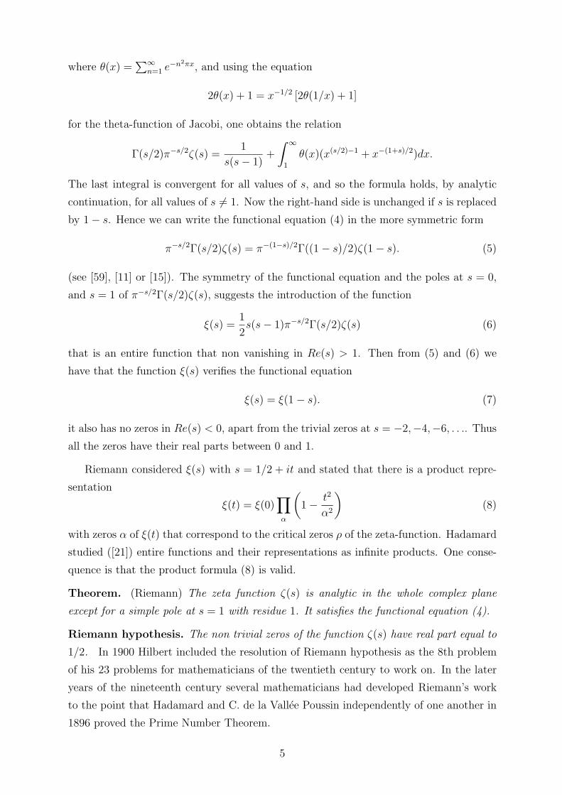
where θ(x) =∑∞

n=1 e−n2πx, and using the equation

2θ(x) + 1 = x−1/2 [2θ(1/x) + 1]

for the theta-function of Jacobi, one obtains the relation

Γ(s/2)π−s/2ζ(s) =1

s(s − 1)+

∫ ∞

1

θ(x)(x(s/2)−1 + x−(1+s)/2)dx.

The last integral is convergent for all values of s, and so the formula holds, by analytic

continuation, for all values of s = 1. Now the right-hand side is unchanged if s is replaced

by 1 − s. Hence we can write the functional equation (4) in the more symmetric form

π−s/2Γ(s/2)ζ(s) = π−(1−s)/2Γ((1 − s)/2)ζ(1 − s). (5)

(see [59], [11] or [15]). The symmetry of the functional equation and the poles at s = 0,

and s = 1 of π−s/2Γ(s/2)ζ(s), suggests the introduction of the function

ξ(s) =1

2s(s − 1)π−s/2Γ(s/2)ζ(s) (6)

that is an entire function that non vanishing in Re(s) > 1. Then from (5) and (6) we

have that the function ξ(s) verifies the functional equation

ξ(s) = ξ(1 − s). (7)

it also has no zeros in Re(s) < 0, apart from the trivial zeros at s = −2,−4,−6, . . .. Thus

all the zeros have their real parts between 0 and 1.

Riemann considered ξ(s) with s = 1/2 + it and stated that there is a product repre-

sentation

ξ(t) = ξ(0)∏α

(1 − t2

α2

)(8)

with zeros α of ξ(t) that correspond to the critical zeros ρ of the zeta-function. Hadamard

studied ([21]) entire functions and their representations as infinite products. One conse-

quence is that the product formula (8) is valid.

Theorem. (Riemann) The zeta function ζ(s) is analytic in the whole complex plane

except for a simple pole at s = 1 with residue 1. It satisfies the functional equation (4).

Riemann hypothesis. The non trivial zeros of the function ζ(s) have real part equal to

1/2. In 1900 Hilbert included the resolution of Riemann hypothesis as the 8th problem

of his 23 problems for mathematicians of the twentieth century to work on. In the later

years of the nineteenth century several mathematicians had developed Riemann’s work

to the point that Hadamard and C. de la Vallee Poussin independently of one another in

1896 proved the Prime Number Theorem.

5

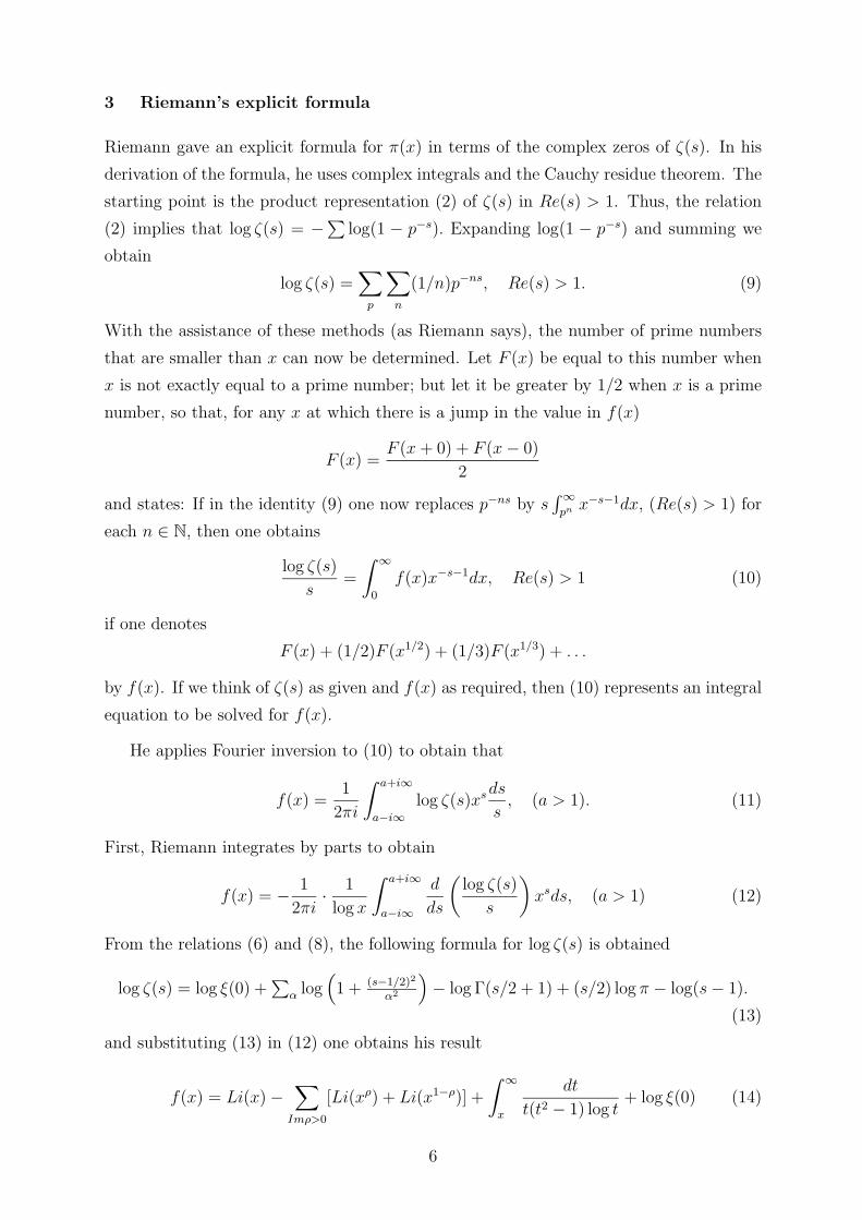
3 Riemann’s explicit formula

Riemann gave an explicit formula for π(x) in terms of the complex zeros of ζ(s). In his

derivation of the formula, he uses complex integrals and the Cauchy residue theorem. The

starting point is the product representation (2) of ζ(s) in Re(s) > 1. Thus, the relation

(2) implies that log ζ(s) = −∑

log(1 − p−s). Expanding log(1 − p−s) and summing we

obtain

log ζ(s) =∑

p

∑n

(1/n)p−ns, Re(s) > 1. (9)

With the assistance of these methods (as Riemann says), the number of prime numbers

that are smaller than x can now be determined. Let F (x) be equal to this number when

x is not exactly equal to a prime number; but let it be greater by 1/2 when x is a prime

number, so that, for any x at which there is a jump in the value in f(x)

F (x) =F (x + 0) + F (x − 0)

2

and states: If in the identity (9) one now replaces p−ns by s∫ ∞

pn x−s−1dx, (Re(s) > 1) for

each n ∈ N, then one obtains

log ζ(s)

s=

∫ ∞

0

f(x)x−s−1dx, Re(s) > 1 (10)

if one denotes

F (x) + (1/2)F (x1/2) + (1/3)F (x1/3) + . . .

by f(x). If we think of ζ(s) as given and f(x) as required, then (10) represents an integral

equation to be solved for f(x).

He applies Fourier inversion to (10) to obtain that

f(x) =1

2πi

∫ a+i∞

a−i∞log ζ(s)xs ds

s, (a > 1). (11)

First, Riemann integrates by parts to obtain

f(x) = − 1

2πi· 1

log x

∫ a+i∞

a−i∞

d

ds

(log ζ(s)

s

)xsds, (a > 1) (12)

From the relations (6) and (8), the following formula for log ζ(s) is obtained

log ζ(s) = log ξ(0) +∑

α log(1 + (s−1/2)2

α2

)− log Γ(s/2 + 1) + (s/2) log π − log(s − 1).

(13)

and substituting (13) in (12) one obtains his result

f(x) = Li(x) −∑

Imρ>0

[Li(xρ) + Li(x1−ρ)] +

∫ ∞

x

dt

t(t2 − 1) log t+ log ξ(0) (14)

6

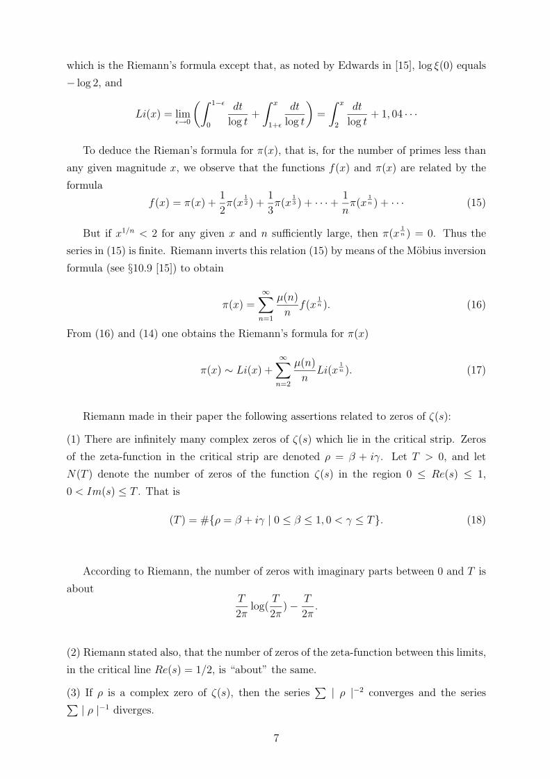
which is the Riemann’s formula except that, as noted by Edwards in [15], log ξ(0) equals

− log 2, and

Li(x) = limε→0

(∫ 1−ε

0

dt

log t+

∫ x

1+ε

dt

log t

)=

∫ x

2

dt

log t+ 1, 04 · · ·

To deduce the Rieman’s formula for π(x), that is, for the number of primes less than

any given magnitude x, we observe that the functions f(x) and π(x) are related by the

formula

f(x) = π(x) +1

2π(x

12 ) +

1

3π(x

13 ) + · · · + 1

nπ(x

1n ) + · · · (15)

But if x1/n < 2 for any given x and n sufficiently large, then π(x1n ) = 0. Thus the

series in (15) is finite. Riemann inverts this relation (15) by means of the Mobius inversion

formula (see §10.9 [15]) to obtain

π(x) =∞∑

n=1

µ(n)

nf(x

1n ). (16)

From (16) and (14) one obtains the Riemann’s formula for π(x)

π(x) ∼ Li(x) +∞∑

n=2

µ(n)

nLi(x

1n ). (17)

Riemann made in their paper the following assertions related to zeros of ζ(s):

(1) There are infinitely many complex zeros of ζ(s) which lie in the critical strip. Zeros

of the zeta-function in the critical strip are denoted ρ = β + iγ. Let T > 0, and let

N(T ) denote the number of zeros of the function ζ(s) in the region 0 ≤ Re(s) ≤ 1,

0 < Im(s) ≤ T . That is

(T ) = #ρ = β + iγ | 0 ≤ β ≤ 1, 0 < γ ≤ T. (18)

According to Riemann, the number of zeros with imaginary parts between 0 and T is

aboutT

2πlog(

T

2π) − T

2π.

(2) Riemann stated also, that the number of zeros of the zeta-function between this limits,

in the critical line Re(s) = 1/2, is “about” the same.

(3) If ρ is a complex zero of ζ(s), then the series∑

| ρ |−2 converges and the series∑| ρ |−1 diverges.

7

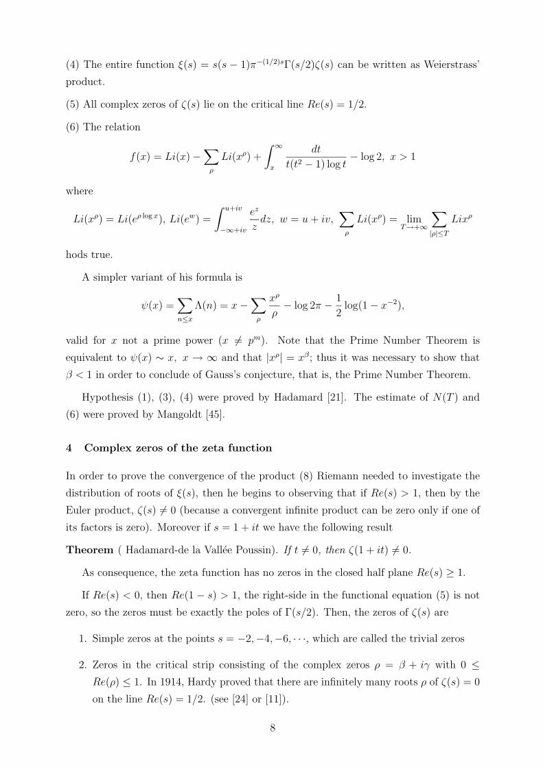
(4) The entire function ξ(s) = s(s − 1)π−(1/2)sΓ(s/2)ζ(s) can be written as Weierstrass’

product.

(5) All complex zeros of ζ(s) lie on the critical line Re(s) = 1/2.

(6) The relation

f(x) = Li(x) −∑

ρ

Li(xρ) +

∫ ∞

x

dt

t(t2 − 1) log t− log 2, x > 1

where

Li(xρ) = Li(eρ log x), Li(ew) =

∫ u+iv

−∞+iv

ez

zdz, w = u + iv,

∑ρ

Li(xρ) = limT→+∞

∑|ρ|≤T

Lixρ

hods true.

A simpler variant of his formula is

ψ(x) =∑n≤x

Λ(n) = x −∑

ρ

xρ

ρ− log 2π − 1

2log(1 − x−2),

valid for x not a prime power (x = pm). Note that the Prime Number Theorem is

equivalent to ψ(x) ∼ x, x → ∞ and that |xρ| = xβ; thus it was necessary to show that

β < 1 in order to conclude of Gauss’s conjecture, that is, the Prime Number Theorem.

Hypothesis (1), (3), (4) were proved by Hadamard [21]. The estimate of N(T ) and

(6) were proved by Mangoldt [45].

4 Complex zeros of the zeta function

In order to prove the convergence of the product (8) Riemann needed to investigate the

distribution of roots of ξ(s), then he begins to observing that if Re(s) > 1, then by the

Euler product, ζ(s) = 0 (because a convergent infinite product can be zero only if one of

its factors is zero). Moreover if s = 1 + it we have the following result

Theorem ( Hadamard-de la Vallee Poussin). If t = 0, then ζ(1 + it) = 0.

As consequence, the zeta function has no zeros in the closed half plane Re(s) ≥ 1.

If Re(s) < 0, then Re(1 − s) > 1, the right-side in the functional equation (5) is not

zero, so the zeros must be exactly the poles of Γ(s/2). Then, the zeros of ζ(s) are

1. Simple zeros at the points s = −2,−4,−6, · · ·, which are called the trivial zeros

2. Zeros in the critical strip consisting of the complex zeros ρ = β + iγ with 0 ≤Re(ρ) ≤ 1. In 1914, Hardy proved that there are infinitely many roots ρ of ζ(s) = 0

on the line Re(s) = 1/2. (see [24] or [11]).

8

Since ζ(s) = ζ(s), the zeros of ζ(s) lie symmetrically with respect to the real axis, so,

it suffices to consider the zeros in the upper half of the critical strip. It is common to list

the complex zeros ρn = βn + iγn, with γn > 0, in order of increasing imaginary parts as

γ1 ≤ γ2 ≤ γ3 ≤ · · · . Here zeros are repeated according to their multiplicity.

Van de Lune, te Riele and Winter [44] have determined that the first 1.500.000.001 com-

plex zeros of ζ(s) are all simple, lie on the critical line, and have imaginary part with

0 < γ < 545.439.823, 215.

(i) Let T > 0, and let N(T ) denote the number of zeros of the function ζ(s) in the region

0 ≤ Re(s) ≤ 1, 0 < Im(s) ≤ T . That is

N(T ) = #ρ = β + iγ | 0 < β ≤ 1, 0 < γ ≤ T.

By the functional equation and the argument principle, one obtains

N(T ) =T

2πlog(

T

2πe) +

7

8+ S(T ) + O(

1

T) (19)

where S(T ) = 1π

arg ζ(12+iT ) log T with the argument obtained by continuous variation

from 2 to 2 + iT , and thence to 1/2 + iT , along straight lines. It was conjectured by

Riemann and proved by von Mangoldt. This is the so called Riemann-von Mangoldt

formula, (the sign of I.M. Vinogradov is taken, as usual, in the sense O).

If the Riemann hypothesis (henceforth RH for short) is true, then it is known that

S(T ) =1

πarg ζ(

1

2+ iT ) log T

log log T. (20)

(ii) Now, let N0(T ) be the zero counting function

N0(T ) = #ρ = 1/2 + iγ | 0 < γ ≤ T,

that it, N0(T ) counts the number of zeros of ζ(s) in the critical line, up to height T . The

RH is equivalent to N(T ) = N0(T ) for all T .

(iii) Let N(σ, T ) the function which counts the number of zeros of ζ(s) in the critical strip

up to height T , and to the right of σ-line.

A method to approach Riemann’s hypothesis is to estimate for any given σ, 1/2 ≤σ ≤ 1, the number N(σ, T ) of zeros ρ = β + iγ of ζ(s), with σ ≤ β and 0 < t ≤ T ( where

T is sufficiently large):

N(σ, T ) = #ρ = β + iγ | β ≥ σ, 0 < γ ≤ T

1/2 ≤ σ ≤ 1. In this case, the RH is equivalent to the property N(1/2, T ) = 0 for all T .

9

Estimates for N(σ, T ) may be written in the form

N(σ, T ) T a(σ)(1−σ) logb T, b ≥ 0. (21)

In view of formula (19) one has a(σ)(1 − σ) = 1 and b = 1 in (21) for 0 ≤ σ ≤ 1/2, while

a(σ)(1 − σ) ≤ 1 for σ > 1/2 and a(σ)(1 − σ) is non increasing.

The hypothesis a(σ) ≤ 2 in (21) is known as “the density hypothesis”. A. Selberg [57]

has proved that

N(σ, T ) T 1− 14(σ− 1

2) log T (22)

uniformly for 1/2 < σ ≤ 1. The RH is equivalent to N(σ, T ) = 0 for σ > 1/2.

Gaps between zeros. The most detailed study of the zeros on the critical line involves

estimates for the difference γn+1−γn between the ordinates of consecutive zeros s = 12+iγ,

γ ∈ R. For a long time, the result of Hardy and Littlewood (1918) that γn+1 − γn γ

1/4+εn was the best. Later it was superseded, with the use of finer methods by Moser,

Balasubramanian, Karatzsuba, Ivic [31].

It is known that the average size of γn+1 − γn is ∼ 2π/ log γn. Thus if

λ := lim supn→∞

(γn+1 − γn)log γn

2π, µ := lim inf

n→∞(γn+1 − γn)

log γn

2π

we have µ ≤ 1 ≤ λ, and it is known (unconditionally) that µ < 1 < λ. It is conjectured

that µ = 0 and λ = ∞, but assuming the generalized RH Conrey-Ghosh- Gonek [9]

proved only that λ > 2.68. Also under the RH they had proved µ < 0.5172.

If (20) holds, then from the estimate (19) one obtains

N(T + H) − N(T ) > 0, for H = C/ log log T, C > 0, T ≥ T0.

Hence assuming the RH the following estimate holds

γn+1 − γn 1

log log γn.

Instead of working with the complex zeros of ζ(s) on the critical line Re(s) = 1/2, it

is convenient to introduce the function

Z(t) = χ−1/2(1

2+ it)ζ(

1

2+ it)

where χ(s) is given by χ(s) = 2sπs−1 sin(πs/2)Γ(1 − s). As χ(s)χ(1 − s) = 1 and Γ(s) =

Γ(s), it follows that | Z(t) |=| ζ(12

+ it) |, Z(t) is even, and Z(t) = Z(t). Hence Z(t) is

real if t is real and the zeros of Z(t) correspond to the zeros of ζ(s) on the critical line

Re(s) = 1/2.

10

5 Consequences of the Riemann hypothesis

There are many equivalent forms for the Riemann hypothesis. The study and classification

of these assertions sharpens our understanding of the problem. Writing Ξ(t) = ξ(1/2+it),

and as consequence of the functional equation (7), we obtain Ξ(t) = Ξ(−t) which is real

for real t an even function of t. Then RH is the assertion to all zeros of Ξ(t) are reals.

Riemann obtained that Ξ(t) verifies the relation

Ξ(t) = 4

∫ ∞

1

d[x3/2θ′(x)]

dxx−1/4 cos

(t

2log x

)dx (23)

where θ(x) =∑∞

n=1 e−n2πx. We can write (23) in the form

Ξ(t) = 2

∫ ∞

0

φ(u) cos ut du

where φ(u) = 2∑∞

n=1(2n4π2e9t/2 − 3n2πe5t/2)e−πn2e2t

. A necessary and sufficiently condi-

tion to of zeros of Ξ(t) are reals is

∫ ∞

−∞

∫ ∞

−∞φ(α)φ(β)ei(α+β)xe(α−β)y(α − β)2dαdβ ≥ 0

for all x, y reals (see Chap X and XIV of [60]).

A. Speiser [58], proved that RH is equivalent to the non-vanishing of the derivate ζ ′(s)

in the left-half of the critical strip 0 < σ < 1/2.

The order of zeta-function on the critical line. Hardy and Littlewood proved that

ζ(1/2 + it) t14+ε for every positive ε, and t ≥ t0 > 0 (since ζ(1/2 + it) = ζ(1/2 − it), t

may be assumed to be positive. H. Weyl improved the bound to t1/6+ε, Bombieri-Iwaniec

obtained 9/56, instead to 1/6, A. Watt improved the bound to 89/560 and M.N. Huxley

([29]) improved the bound to

ζ(1/2 + it) t89570

+ε.

Lindelof conjectured that

ζ(1/2 + it) ε tε, t ≥ t0 > 0

for every positive ε. In 1912, Littlewood proved that the Lindelof hypothesis is true if the

RH is true. The converse theorem cannot be made.

For the function S(T ) = 1π

arg ζ(12

+ iT ) we have that the LH is equivalent to

∫ T

0

S(t)dt = o(log T ), (T → ∞)

11

while the RH implies much more

∫ T

0

S(t)dt log T

log log T, (T → ∞).

The order of zeta-function on the 1-line. E.C. Titchmarsh, was proved ([60] theorems

8.5 and 8.8), that each one of the inequalities

| ζ(1 + it) |> A log log t, 1/ | ζ(1 + it) |> A log log t

is satisfies for some arbitrary large values of t, if A is a suitable constant and considers

the question of how large the constant can be in the two cases.

On RH we have

eγ ≤ lim supt→∞

ζ(1 + it)

log log t≤ 2eγ

6

π2eγ ≤ lim sup

t→∞

1/ζ(1 + it)

log log t≤ 12

π2eγ

where γ is Euler’s constant, (see Titchmarsh [60] 8.9).

Riemann hypothesis and distribution of primes. We know that the zeta function

was introduced as an analytic tool for studying prime numbers and some of the most

important applications of the zeta functions belong to prime number theory. The equiv-

alence between the error term in the Prime Number Theorem and the real part of the

zeros of ζ(s) is as follow

π(x) =

∫ x

2

dt

log t+ O(xθ+ε)

or

ψ(x) =∑

pm≤x

log p = x + O(xθ log2 x)

is equivalent to ζ(s) = 0 for Re(s) > θ, 1/2 ≤ θ < 1 (Th. 12.3 [31]). If we use the

strongest zero-free region then we deduce the results

π(x) −∫ x

2

dt

log t x1/2 exp(−C(log x)3/5(log log x)−1/5)

ψ(x) − x x1/2 exp(−C(log x)3/5(log log x)−1/5)

but the Riemann hypothesis is equivalent to each of the following statements related to

prime numbers

(1) π(x) =∫ x

2dt

log t+ O(

√x log x). [35]

(2) ψ(x) =∑

pm≤x log p = x + O(√

x log2 x), x > 0.

In the problem related to the difference of two consecutive prime numbers, Pilts conjec-

tured that for every ε > 0, pn+1−pn pεn where pn denote the nth prime number, but this

12

has never been proved. On the other hand, it is known that the relation pn+1−pn log pn

is certainly not true.

(3) The RH is equivalent to pn+1 − pn p1/2n log pn.

The Mobius function. The Euler product formula for ζ(s) implies that

1

ζ(s)=

∏p

1 − p−s =∞∑

n=1

µ(n)

ns, s = σ + it, σ > 1.

The coefficient µ(n) is known as Mobius function.

It has the property∑

d|n µ(d) = 1, (n = 1) and 0 if n > 1, where d|n means that d is

a divisor of n. Thus µ(n) verifies

µ(1) = 1, µ(n) = −∑

d|n,d<n

µ(d), (n > 1).

Each one of the following properties is equivalent to the RH (see [60])

(4) M(x) =∑

n≤x µ(n) x1/2+ε, for all ε > 0,

(5) the series∑∞

n=1 µ(n)/n−s is convergent, and its sum is 1/ζ(s), for every s with

σ > 1/2.

The function w(n). Let ω(n) be the number of prime factors of the positive integer n

counted without multiplicity, and q ∈ N. D. Wolke proved that the RH is true if and

only if ∑n≤x

ωq(n) − x∑

0≤j≤ 12

log x

Rjq(log log x)(log x)−j x1/2+ε

holds for every ε > 0, where Rjq(t) are certain polynomials such that deg R0q ≤ q, and

deg Rjq ≤ q − 1, (j ≥ 1) (see [63]).

Sum of divisors. Let σ(n) denote the sum of divisors of n, that is σ(n) =∑

d|n d. G.

Robin (see[54]) proved that RH is true, if and only if

σ(n) < eγn log log n

for large n, where γ is the Euler’s constant. J.C. Lagarias [39], proved that under the RH

σ(n) < Hn + eHn log Hn, Hn =n∑

j=1

1/j, (n ≥ 2).

Bertrand’s postulate. In 1852, Chebyshev proved Bertrand’s postulate according to

which each interval (n, 2n], n ≥ 1, contains at least one prime. O. Romare, Y. Saoutier

13

[55] under the RH proved that for all x ≥ 2 in the interval (x − 85

√x log x, x] there exist

a prime number.

Pythagorean triangles. The positive integers a, b, c are said to form a primitive

Pythagorean triples (a, b, c) if a ≤ b, a, b, c are coprimes and a2 + b2 = c2. Let P (x)

denote the number of primitive Pythagorean triangles, whose area is less than x. In

1955, J. Lambek y L. Moser [Pacific J. Math. 5(1955), 73-83, MR 16, 796h] proved that

P (x) = c1x1/2 +O(x1/3). Muler, Nowak and Menzer ([50]), assuming the RH proved that

P (x) = c1x1/2 + c2x

1/3 + R(x), with R(x) x127/560+ε. The error term is connected with

the Mobius function and then with the zeros of the zeta function. W. Zhai [70] under the

RH deduced

R(x) x127/616(log x)963/308, 127/616 = 0.2061 . . .

A Divisor problem. Let a, b be positive coprime integers such that 1 ≤ a < b, and let

∆a,b(x) be the error term for the asymptotic formula of

D∗(a, b; x) =∑

manb≤x, (m,n)=1

1, (1 ≤ a < b, (a, b) = 1.

Lu y Zhai [43], proved under the RH that

∆a,b(x) xa+6b

(2a+7b)(a+b)+ε, b ≤ 3a

2; ∆a,b(x) x

a+2b(2a+2b)(a+b)

+ε, b >3a

2.

The primitive circle problem. Let

P (x) =∑

m2+n2≤x,(m,n)=1

1

and let ∆(x) = P (x) − (6/π)x. The ”primitive circle problem” is to obtain an upper

bound for ∆(x). The best known unconditional result is

∆(x) x1/2 exp(−c(log x)3/5(log log x)−1/5).

Jie Wu ([68]), under the Riemann hypothesis proved that ∆(x) x221/608+ε.

Powerful numbers. Let k ≥ 2 be a fixed integer and let Nk denote the set of all positive

integers n with the property that if a prime p | n, then pk | n. Thus the set of powerful

numbers Nk contains 1 and the numbers whose canonical representation is n = pα11 · · · pαr

r ,

αi ≥ k for all i = 1, 2, · · · , r. We put fk(n) = 1 if n ∈ Nk and fk(n) = 0 if n ∈ Nk and

the Dirichlet series representation is

Fk(s) =∞∑

n=1

fk(n)n−s =∏

p

(1 +p−ks

1 − p−s), Re(s) > 1/k,

14

then fk(n) is the characteristic function of Nk, (see E. Kratzel [36] Chap. 7). The problem

is to obtain an estimate for the number Nk(x) of k-full integers not exceeding x:

Nk(x) =∑n≤x

fk(n), k ≥ 2

the main term is deduced from the residues of Fk(s) at the simples poles s = 1/u,

u = k, k + 1, · · · , 2k − 1 and we have the following relation

Nk(x) =2k−1∑t=k

ct,kx1/k + ∆k(x), ct,k = Res

s=1/tFk(s)/s.

Let γk = infρk | ∆k(x) xρk. A. Ivic showed that we would have under the

assumption of the truth of Lindelof hypothesis, γk ≤ 1/2k, but in special cases, it is

possible to prove much more. If k = 2, we have

F2(s) =ζ(2s)ζ(3s)

ζ(6s).

Let N2(x) be denote the number of square-full integers n ≤ x, and ∆2(x) the error

term. The best unconditional O-estimate is

∆2(x) = N2(x) − ζ(3/2)

ζ(3)x

12 − ζ(2/3)

ζ(2)x

13 x

16 exp(−c(log x)

35 (log log x)−

15 ),

essentially due to P. T. Bateman and E. Grosswald [3] see Theorem 14.4 and page 438 in

A. Ivic’s book [31].

Under the RH, J. Wu [67] proved that ∆2(x) x(12/85)+ε, for any ε > 0, which can be

compared with the complementary estimate ∆(x) = Ω(x1/10), due to R. Balasubramanian,

K. Ramachandra and M. V. Subbarao (Acta Arith. 50 (1988), no. 2, 107-118). Bateman

and Grosswald also noted that the statement ∆2(x) xα, for any constant exponent

α < 1/6, is equivalent to some quasi-Riemann hypothesis, i.e. to the assertion that

ζ(s) = 0 for all s with σ > σ0 and σ0 < 1.

A similar situation arises in case of cube-full integers.

Farey series and the RH. A sequence (xn) of real numbers is uniformly distributed

(mod 1) if and only if for every Riemann-integrable function f on [0, 1] one has

limN→∞

1

N

∑n≤N

f(xn) =

∫ 1

0

f(x)dx

where x is the fractional part of x, ([10], Th. 3 Cahp. VIII). Let Fx = F[x] denote the

sequence of all irreducible fractions with denominators ≤ x, arranged in increasing order

of magnitude, that is

15

Fx = rk = ak/bk; 0 < ak ≤ bk ≤ x, (ak, bk) = 1, k = 1, 2, · · · , φ(x), for any x ≥ 1, where

φ(x) =∑

n≤x ϕ(n), (ϕ(n) = #k ≤ n; (k, n) = 1 is the Euler function. F[x] is called

the Farey series of order x, (Note that the Farey series is not a series at all but a finite

sequence).

Since the Farey fractions are uniformly distributed (mod 1) we have that

limN→∞

1

φ(N)

∑q≤N

q∑a=1

(a,q)=1

f(a/q) =

∫ 1

0

f(x)dx (24)

for every Riemann-integrable function f on [0, 1]. Relation (24) suggests the problem of

estimation of the error term

Ef (N) =∑q≤N

q∑a=1

(a,q)=1

f(a/q) − φ(N)

∫ 1

0

f(x)dx.

Franel discovered a connection between Farey series and the Riemann hypothesis. He

proved ( [17]) that the estimation

∑k≤φ(x)

(rk −

k

φ(x)

)2

ε x2(β−1)+ε

for every ε > 0 is equivalent to ζ(s) = 0 for Re(s) > β. Thus

RH is truth if and only if

∑k≤φ(x)

(rk −

k

φ(x)

)2

x−1+ε.

Another version (Landau Vorlesungen ii, 167-177), is that the RH is equivalent to

the statement ∑k≤φ(x)

| rk −k

φ(x)| x

12+ε,

for all ε > 0 as x → ∞.

M. Mikolas, (see [46]-[49]) proved that the RH is equivalent to the relation

φ(x)∑k=1

f(rk) − φ(x)

∫ 1

0

f(u)du x1/2+ε

for all ε > 0, where f(u) can be sin(λu), cos(λu), (|λ| = π) or a polynomial of degree ≤ 3.

Huxley [28] has generalized Franel’s theorem to the case of Dirichlet L-functions and Fujii

[18] gives another equivalence with the RH in terms of the Farey series.

16

Kanemitsu and Yoshimoto [33] showed that each one of the estimates are equivalent

to the RH

∑rk≤1/3

(rk −

h(1/3)

2φ(x)

) x1/2+ε,

∑rk≤1/4

(rk −

h(1/4)

2φ(x)

) x1/2+ε

where h(t) =∑

rk≤t 1. Moreover, Kanemitsu and Yoshimoto obtain conditions equivalents

for a great class of functions (see also [34], [69]).

The Riesz sum. M. Riesz (see [60]) considers the function

f(x) =∞∑

n=1

(−1)n+1xn

(n − 1)!ζ(2n).

An application of the calculus of residues gives

f(x) =i

2

∫ a+i∞

a−i∞

xsds

Γ(s)ζ(2s) sin(πs)=

i

2π

∫ a+i∞

a−i∞

Γ(1 − s)xsds

ζ(2s),

where 1/2 < a < 1. Taking a > 1/2 it follows that f(x) x1/2+ε. On the RH we can

move the line of integration to a = 1/4 + ε and obtain the estimation f(x) x1/4+ε.

Conversely, by Mellin’s inversion formula

Γ(1 − s)

ζ(2s)= −

∫ ∞

0

f(x)x−s−1dx

and if f(x) x1/4+ε holds, then the integral converges uniformly for σ ≥ σ0 > 1/4, the

analytic function represented is regular for σ > 1/4 and the truth of the RH follows.

Hardy and Littlewood in 1918 [60] stated that RH holds if and only if

∞∑n=1

(−x)n

n!ζ(2n + 1) x−1/4, x → ∞.

Nyman-Beurling criterion. The Riemann zeta function on may see as a Mellin trans-

form in the critical strip by means of the following formula

ζ(s)

s= −

∫ ∞

0

ρ(1/x)xs−1dx, 0 < σ < 1

where ρ(x) is the fractional part function ρ(x) = x − [x].

B. Nyman and A. Beurling had the idea that it should be possible to translate the

Riemann hypothesis into a property of ρ(x). Beurling’s linear space N(0,1) consists of all

functions

x → f(x) =n∑

k=1

akρ(θk

x), 0 < θk ≤ 1

where the ak are constants such that,∑n

k=1 akθk = 0. For 1 < p < ∞, let Bp be the

closure of B in Lp(0, 1). In his thesis, Nyman [51] proved the following theorem:

17

Theorem. The Riemann hypothesis is true if and only if N(0,1) is dense in L2(0, 1).

Beurling gives in his paper [4] a generalization of Nyman’s theorem

Theorem. Let 1 < p < ∞. The following properties are equivalent.

(i) ζ(s) has no zeros in the half plane Re(s) > 1/p

(ii) N(0,1) is dense in Lp(0, 1)

(iii) The characteristic function χ(0,1) is in the closure of N(0,1) in Lp(0, 1).

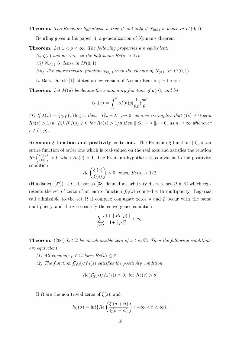
L. Baez-Duarte [1], stated a new version of Nyman-Beurling criterion:

Theorem. Let M(y) be denote the summatory function of µ(n), and let

Gn(x) =

∫ n

1

M(θ)ρ(1

θx)dθ

θ.

(1) If λ(x) = χ(0,1)(x) log x, then ‖ Gn − λ ‖p→ 0, as n → ∞ implies that ζ(s) = 0 para

Re(s) > 1/p. (2) If ζ(s) = 0 for Re(s) > 1/p then ‖ Gn − λ ‖r→ 0, as n → ∞ whenever

r ∈ (1, p).

Riemann ξ-function and positivity criterion. The Riemann ξ-function (6), is an

entire function of order one which is real-valued on the real axis and satisfies the relation

Re(

ξ′(s)ξ(s)

)> 0 when Re(s) > 1. The Riemann hypothesis is equivalent to the positivity

condition

Re

(ξ′(s)

ξ(s)

)> 0, when Re(s) > 1/2.

(Hinkkanen [27]). J.C. Lagarias [38] defined an arbitrary discrete set Ω in C which rep-

resents the set of zeros of an entire function fΩ(z) counted with multiplicity. Lagarias

call admissible to the set Ω if complex conjugate zeros ρ and ρ occur with the same

multiplicity, and the zeros satisfy the convergence condition

∑ρ∈Ω

1+ | Re(ρ) |1+ | ρ |2 < ∞.

Theorem. ([38]) Let Ω be an admissible zero of set in C. Then the following conditions

are equivalent

(1) All elements ρ ∈ Ω have Re(ρ) ≤ θ

(2) The function f ′Ω(s)/fΩ(s) satisfies the positivity condition

Re(f ′Ω(s)/fΩ(s)) > 0, for Re(s) > θ.

If Ω are the non trivial zeros of ζ(s), and

hQ(σ) = infRe

(ξ′(σ + it)

ξ(σ + it)

): −∞ < t < ∞,

18

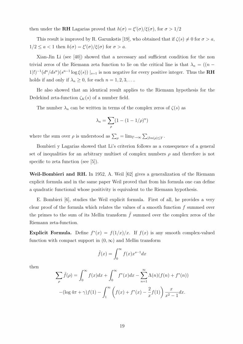
then under the RH Lagarias proved that h(σ) = ξ′(σ)/ξ(σ), for σ > 1/2

This result is improved by R. Garunkstis [19], who obtained that if ζ(s) = 0 for σ > a,

1/2 ≤ a < 1 then h(σ) = ξ′(σ)/ξ(σ) for σ > a.

Xian-Jin Li (see [40]) showed that a necessary and sufficient condition for the non

trivial zeros of the Riemann zeta function to lie on the critical line is that λn = ((n −1)!)−1(dn/dsn)(sn−1 log ξ(s)) |s=1 is non negative for every positive integer. Thus the RH

holds if and only if λn ≥ 0, for each n = 1, 2, 3, . . ..

He also showed that an identical result applies to the Riemann hypothesis for the

Dedekind zeta-function ζK(s) of a number field.

The number λn can be written in terms of the complex zeros of ζ(s) as

λn =∑

ρ

(1 − (1 − 1/ρ)n)

where the sum over ρ is understood as∑

ρ = limT→∞∑

|Im(ρ)≤T .

Bombieri y Lagarias showed that Li’s criterion follows as a consequence of a general

set of inequalities for an arbitrary multiset of complex numbers ρ and therefore is not

specific to zeta function (see [5]).

Weil-Bombieri and RH. In 1952, A. Weil [62] gives a generalization of the Riemann

explicit formula and in the same paper Weil proved that from his formula one can define

a quadratic functional whose positivity is equivalent to the Riemann hypothesis.

E. Bombieri [6], studies the Weil explicit formula. First of all, he provides a very

clear proof of the formula which relates the values of a smooth function f summed over

the primes to the sum of its Mellin transform f summed over the complex zeros of the

Riemann zeta-function.

Explicit Formula. Define f ∗(x) = f(1/x)/x. If f(x) is any smooth complex-valued

function with compact support in (0,∞) and Mellin transform

f(x) =

∫ ∞

0

f(x)xs−1dx

then ∑ρ

f(ρ) =

∫ ∞

0

f(x)dx +

∫ ∞

0

f ∗(x)dx −∞∑

n=1

Λ(n)(f(n) + f ∗(n))

−(log 4π + γ)f(1) −∫ ∞

1

(f(x) + f ∗(x) − 2

xf(1)

)x

x2 − 1dx.

19

Bombieri next proves a strong version of Weil’s criterion for the Riemann hypothesis.

One takes a function f(x) = g ∗ g∗ in the Weil formula, where ∗ is the multiplicative

convolution of a function g and its transpose conjugate g∗.

Theorem (Bombieri). The Riemann Hypothesis holds if and only if

∑ρ

g(ρ)g(1 − ρ) > 0

for every complex-valued g(x) ∈ C∞0 ((0,∞)), not identically 0.

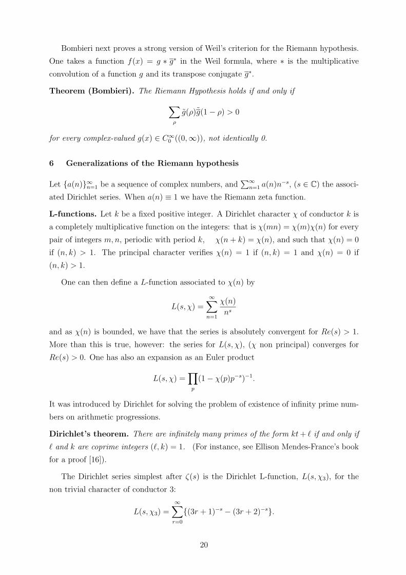
6 Generalizations of the Riemann hypothesis

Let a(n)∞n=1 be a sequence of complex numbers, and∑∞

n=1 a(n)n−s, (s ∈ C) the associ-

ated Dirichlet series. When a(n) ≡ 1 we have the Riemann zeta function.

L-functions. Let k be a fixed positive integer. A Dirichlet character χ of conductor k is

a completely multiplicative function on the integers: that is χ(mn) = χ(m)χ(n) for every

pair of integers m, n, periodic with period k, χ(n + k) = χ(n), and such that χ(n) = 0

if (n, k) > 1. The principal character verifies χ(n) = 1 if (n, k) = 1 and χ(n) = 0 if

(n, k) > 1.

One can then define a L-function associated to χ(n) by

L(s, χ) =∞∑

n=1

χ(n)

ns

and as χ(n) is bounded, we have that the series is absolutely convergent for Re(s) > 1.

More than this is true, however: the series for L(s, χ), (χ non principal) converges for

Re(s) > 0. One has also an expansion as an Euler product

L(s, χ) =∏

p

(1 − χ(p)p−s)−1.

It was introduced by Dirichlet for solving the problem of existence of infinity prime num-

bers on arithmetic progressions.

Dirichlet’s theorem. There are infinitely many primes of the form kt + if and only if

and k are coprime integers (, k) = 1. (For instance, see Ellison Mendes-France’s book

for a proof [16]).

The Dirichlet series simplest after ζ(s) is the Dirichlet L-function, L(s, χ3), for the

non trivial character of conductor 3:

L(s, χ3) =∞∑

r=0

(3r + 1)−s − (3r + 2)−s.

20

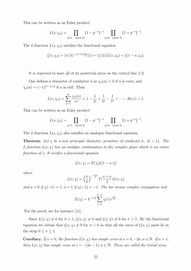
This can be written as an Euler product

L(s, χ3) =∏

p≡1 (mod 3)

1 − p−s−1∏

p≡2 (mod 3)

1 + p−s−1.

The L-function L(s, χ3) satisfies the functional equation

ξ(s, χ3) = (π/3)−(s+1)/2Γ((s + 1)/2))L(s, χ3) = ξ(1 − s, χ3).

It is expected to have all of its nontrivial zeros on the critical line 1/2.

One defines a character of conductor 4 as χ4(n) = 0 if n is even; and

χ4(n) = (−1)(n−1)/2 if n is odd. Then

L(s, χ4) =∞∑

n=1

χ4(n)

ns= 1 − 1

3s+

1

5s− 1

7s+ · · · , Re(s) > 1.

This can be written as an Euler product

L(s, χ4) =∏

p≡1 (mod 4)

1 − p−s−1∏

p≡3 (mod 4)

1 + p−s−1.

The L-function L(s, χ4) also satisfies an analogue functional equation.

Theorem. Let χ be a non principal character, primitive of conductor k, (k > 1). The

L-function L(s, χ) has an analytic continuation to the complex plane which is an entire

function of s. It verifies a functional equation

ξ(s, χ) = E(χ)ξ(1 − s, χ)

where

ξ(s, χ) =(π

k

)− s+a2

Γ(s + a

2)L(s, χ)

and a = 0 if χ(−1) = 1; a = 1 if χ(−1) = −1. The bar means complex conjugation and

E(χ) = k−1/2

k−1∑r=1

χ(r)e2πik .

For the proof, see for instance [11].

Since L(s, χ) = 0 for σ > 1, ξ(s, χ) = 0 and ξ(s, χ) = 0 for σ > 1. By the functional

equation we obtain that ξ(s, χ) = 0 for σ < 0 so that all the zeros of ξ(s, χ) must lie in

the strip 0 ≤ σ ≤ 1.

Corollary. If a = 0, the function L(s, χ) has simple zeros at s = 0,−2n, n ∈ N. If a = 1,

then L(s, χ) has simple zeros at s = −(2n− 1), n ∈ N. These are called the trivial zeros.

21

As in the case of ζ(s), one can deduce the existence of an infinity of non-real zeros

of L(s, χ) either by using to the theory of entire functions, or by an estimate of the

Riemann-von Mangoldt type. One can prove that if N(T ) denotes the number of zeros

ρ = β + iγ, 0 < β < 1, 0 < γ ≤ T of L(s, χ) then

N(T ) =T

2πlog T + AT + O(log T )

where A is a constant which depends on k, the modulus of character χ.

The theorem of the existence of an infinity of zeros of the critical line, proved by

Hardy for the ζ(s), has been extended to a general class of Dirichlet series, including the

L-functions, by E. Hecke.

Generalized Riemann Hypothesis. The conjecture is that all the zeros of L-functions

are situated on the critical line.

Let(

dn

)denote Kronecker’s extension of the Legendre symbol for quadratic residues,

for n = 1, 2, · · ·. It is known that if d is the discriminant of a quadratic number field (that

is, d is square-free and d ≡ 1 (mod 4); or d = 4N where N ≡ 2 or 3 (mod 4), and

square-free), and χd(n) =(

dn

), then χd is a real primitive Dirichlet character modulus

| d |. Let

L(s, χd) =∞∑

n=1

χd(n)n−s

be the associated Dirichlet L-function. It is an entire function (for d = 1) which satisfies

the functional equation

ξ(s, χd) =

(π

| d |

)−s/2

Γ

(s + ad

2

)L(s, χd) = ξ(1 − s, χd)

where ad = 1 if d < 0 and ad = 0 if d > 0.

Zeta functions of number field. For a number field K of degree n, the zeta function

of K is

ζK(s) =∞∑

m=1

FK(m)

ms,

where FK(m) is the number of ideals whose norm is precisely m. This sum converges

for complex s with Re(s) > 1. Often ζK(s) is referred to as the Dedekind zeta function.

When K = Q, is just the Riemann zeta function: ζQ(s) = ζ(s).

The function ζK(s) has an analytic continuation to the entire complex s-plane except

for a first order pole at s = 1. The residue of ζK(s) at s = 1 is

Ress=1ζK(s) =2r1+r2πr2hR

w√

| D |

22

where r1 is the number of real conjugate fields of K, 2r2 is the number of complex conjugate

fields of K, n is the degree of K, h is the class-number of K, R is the regulator of K, w

is the number of roots of unity in K, and D is the discriminant of K. There is also a

functional equation relating values at s = 1 to values at 1 − s,

ξK(s) = ξK(1 − s)

where

ξK(s) =

( | D |22r2πn

)s/2

Γr1(s/2)Γr2(s)ζK(s)

The function ζK(s) has no zeros in Re(s) > 1. It has trivial zeros with Re(s) < 0

of order r2 at −1,−3,−5, . . .; of order r1 + r2 at −2,−4,−6, . . .; and one zero of order

r1 + r2 − 1 at s = 0. All other zeros are in the critical strip. (See [65] chap. 6: Galois

Theory, Algebraic Number Theory, and Zeta Functions from H.M. Stark).

Extended Riemann Hypothesis. The Extended Riemann Hypothesis is the assertion

that the non trivial zeros of Dedekind zeta function of any algebraic number field lie on

the critical line.

Some consequences.

(1) Given the GRH, the Siegel-Walfisz theorem (see Th-5 [59], cap II.8) can be improved

to

ψ(x; h, k) =∑n≤x

n≡h (mod k)

Λ(n) =x

ϕ(k)+ O(

√x log2 x), k ≤ x.

(2) Also we have

π(x; h, k) =∑p≤x

p≡h (mod k)

1 =x

ϕ(k) log x+ O(

√x log x).

(3) D. Wolke (see [64] ), obtained the following equivalence for L-functions: Let χ0, χ1, χ2, . . .

be the sequence of all Dirichlet characters (in which the principal character χ0 occurs

only once), ordered which increasing moduli, and let αkk∈N a sequence of real numbers

αk → 0 for k → ∞ which, in addition, satisfies the condition

∑k∈N

αk log(k + 1) | log αk |< ∞.

Define the multiplicative function f : N → C by

∞∑n=1

f(n)n−s = (ζ(s))−1

∞∏k=1

(L(s, χk))αk , Re(s) > 1

23

then Wolke proved that the GRH in true iff

∑n≤x

f(n) x1/2+ε, for all ε > 0.

(4) The Goldbach conjecture. The three prime Goldbach conjecture states that every odd

integer ≥ 9 is a sum of three odd primes. The conjecture was proved under the GRH by

Deshouillers-Effinger-te Riele-Zinoviev [14].

Quasi Riemann hypothesis. The term “Quasi Riemann hypothesis” related to a zeta-

function is used to mean that this zeta-function has no zeros in a half-plane σ > σ0 for

some σ0 < 1.

Modified Generalized Riemann Hypothesis. Say that an L-function satisfies the

Modified Great Riemann Hypothesis, if its zeros are all on the critical line or the real

axis.

The function ω(n) =∑

p|n 1 has “normal” order log log n and a famous theorem of

Turan bounds the variance of this distribution. Now let fa(n) be the smallest positive

integer m such that am ≡ 1 (mod n), with a relatively prime to n. Saidak ([56]) obtained

results of Turan type for the function ω(fa(n)), thus assuming a quasi-Riemann hypothesis

for the Dedekind zeta functions of certain nonabelian number fields, he proves that for

each squarefree integer a ≥ 2,

∑p≤x(p,a)=1

(ω(fa(p)) − log log p

)2

π(x) log log x

∑n≤x(n,a)=1

(ω(fa(n)) − 1

2(log log n)2

)2

x(log log x)3.

The Ramanujan zeta function. Let

L(s, τ) =∞∑

n=1

τ(n)

ns, σ >

13

2(25)

be the L-function attached to the Ramanujan function τ(n). The function τ(n) is multi-

plicative (proved by Mordell, 1917). The order of magnitude for τ(n) is |τ(n)| ≤ n11/2d(n),

which was conjectured by Ramanujan in 1916 and proved by P. Deligne 60 years later

[13].

The Euler product corresponding to L(s, τ) is

L(s, τ) =∏

p

(1 − τ(p)p−s + p11−2s)−1, (σ >13

2)

24

and the functional equation, becomes

(2π)−sΓ(s)L(s, τ) = (2π)s−12Γ(12 − s)L(12 − s, τ).

It has the trivial zeros s = 0,−1,−2,−3, · · · but no other zeros for σ ≤ 112

and σ ≥ 132.

The critical strip 0 < σ < 1 corresponding to the function ζ(s) is the strip 112

< σ < 132.

The analytic continuation of L(s, τ) has an infinity of zeros on the critical line Re(s) = 6

and the Riemann hypothesis for L(s, τ) asserts that all its complex zeros lie on that line.

The Davenport-Heilbronn zeta function. This function was introduced by H. Dav-

enport and H. Heilbronn as

f(s) = 5−s(ζ(s, 1/5) + tan θζ(s, 2/5) − tan θζ(s, 3/5) − ζ(s, 4/5)) (26)

where

ζ(s, a) =∞∑

n=0

(n + a)−s (0 < a ≤ 1), Re(s) > 1

is the Hurwitz zeta function defined for Re(s) ≤ 1 by analytic continuation. For θ =

arctan((√

10 − 2√

5 − 2)/(√

5 − 1)) it can be shown (see [12] or [60] cap. X), that f(s)

satisfies the functional equation

f(s) = 2 · 5−s+ 12 (2π)s−1Γ(1 − s) cos(

πs

2)f(1 − s).

Moreover f(s) has an infinity of zeros on the line σ = 1/2 and it also has an infinity

of zeros in the half-plane Re(s) > 1, ( ζ(s) = 0 in Re(s) > 1). Thus the function f(s)

of Davenport and H. Heilbronn, satisfies a functional equation similar to the functional

equation for ζ(s), but has no Euler product, and the analogue of the Riemann hypothesis

is FALSE for f(s).

7 Remarks.

The work of Riemann on the distribution of primes is thoroughly studied in Edwards’

book [15], that I recommend strongly (a jewel), but a moderate knowledge of elementary

number theory and complex analysis is required of the reader. I suggest for example to

study the Tenenbaum’s book (also the book of Ellison-Mendes). Another important text

is the great classic book of E.C. Titchmarh with an extensive treatment of the theory

of ζ(s) up to 1951 and its second edition revised by D.R. Heath-Brown (see Chapters

XIII-XV for Riemann Hypothesis). A. Ivic [31] develops the theory of the Riemann zeta-

function and some applications, and the results proved in this text are unconditional, that

is, they do not depend on any hitherto unproved hypothesis.

There are so many results and conjectures having to do with the Riemann hypoth-

esis that it is very difficult to mention all of them. The reader interested on Riemann

hypothesis can consult the Mathematical Reviews with about 1600 references (up today).

25

References

[1] Baez-Duarte, L. New versions of the Nyman-Beurling criterion for the Riemann Hypothesis.

Int. J. Math. Math. sci. 31 (2002), 7, 387-406.

[2] Balazard, M. Completeness problems and the Riemann hypothesis; An annotated bibliogra-

phy. Collection: Number theory for the Milleniunm (2002), 21-48.

[3] Bateman, P.T.; Grosswald, E. On a theorem of Erdos and Szekeres. Illinois-J.-Math. 2

(1958), 88-98.

[4] Beurling, A. A closure problem related to the Riemann zeta-function. Proc. Nat. Acad. Sci.

U.S.A. (1955), 41, 312-314.

[5] Bombieri, E. Lagarias, J.C. Complements to Li’s criterion for the Riemann hypothesis. J.

Number Theory 77, 274-287, (1999).

[6] Bombieri, E. Remarks on Weil’s quadratic functional in the theory of prime numbers, I.

Att. Accad Naz. Licei (9) Mat. Appl. 11 (2000) n-3, 183-233.

[7] Calderon, C. La funcion zeta de Riemann. Rev. Real Academia de Ciencias de Zaragoza.

57, (2002), 67-87.

[8] Conrey,J.B. The Riemann Hypothesis. Not. Amer. Math. Soc. 50 (2003),no. 3, 341-353.

[9] Conrey,J.B.-Ghosh, A.-Gonek,S.M. Large gaps between zeros on the zeta function. Math-

ematika, 33 (1986) 2, 212-338 (1987).

[10] Chandrasekharan, K. Introduction to analytic number theory.Springer Verlag New York

1968.

[11] Chandrasekharan, K. Arithmetical functions. Springer Verlag New York 1969.

[12] Davenport, H.-Heilbrom, H. On the zeros of certain Dirichlet series, I, II.J. London Math.

Soc. 11 (1936), 181-185, 307-312.

[13] Deligne, P. La conjeture de Weil I. I.H.E.S. Publ. Math. 43 (1974), 273-307.

[14] Deshouillers, J.M.-Effinger, G.-te-Riele, H.-Zinoviev, D. A complete Vinogradov 3-primes

theorem under the Riemann hypothesis. Electron Res. Announc. Amer. Math. Soc. 3 (1997),

99-104.

[15] Edwards, H.M. Riemann’s zeta function Acad. Press. New York. 1974.

[16] Ellison, W. J. and Mendes-France, M. Les nombres premiers. Hermann Paris (1975).

[17] Franel, J. Les suites de Farey et le probleme des nombres premiers. Gottinger Nachrichten

(1924), 198-201.

26

[18] Fujii, A. A remark on the Riemann hypothesis. Comment. Math. Univ. St. Paul. 29 (1980),

195-201.

[19] Garunkstis, R. On a positivity property of the Riemann ξ-function Lithuanian Math. Jour-

nal 42 (2002) n-2, 140-145.

[20] Gauss, C.F. Carta a Enke fechada el 24 de Diciembre de 1849, “Werke” Vol.II, pp. 444-447.

Koniglichen Gesellschaft der Wissenchaften zu Gottingen.

[21] Hadamard, J. Etude sur les proprietes des fonctions entieres et en particulier d’une fonction

consideree par Riemann. J. Math. Pures Appl. (4) 9, 171-215 (1893)

[22] —– Sur la distribution des zeros de la fonction ζ(s) et ses consecuences arithmetiques.

Bull. Soc. Math. France 24, 199-220 (1896).

[23] Hardy, G.H. Comptes Rendus, Acad. Sci. Paris, 158 (1914), 1012-1014.

[24] —– Sur les zeros de la function ζ(s) de Riemann. C.R. Acad. Sci. Paris 158, 1012-1014

(1914).

[25] Hardy, G.H. and Wright, E.M. An Introduction to the theory of numbers. Oxford. Clarendon

Press. 1979.

[26] Hardy, G.H.-Littlewood, J.E. Contributions to the theory of the Riemann zeta function and

the distributions of primes. Acta Math. 41, 19-196 (1918).

[27] Hinkkanen, A. On functions of bounded type. Complex Var. Th. Appl. Int. Jour. 34 (1997)

no. 1-2, 119-139.

[28] Huxley, N.M. The distribution of Farey points I. Acta Arith. 18 (1971), 281-287.

[29] —– Exponential sums and the Riemann zeta function IV. Proc. London Math. Soc. (1993)

(3) 66, 1-40

[30] Ingham, A. The distribution of prime numbers. Cambridge University Press, Cambridge,

1932.

[31] Ivic, A. The Riemann zeta function. Jhon Wiley, New York 1985.

[32] —– On some results concerning the Riemann hypothesis.Collection: Analytic number

theory London Math. Soc. Lecture Notes Ser. 247, 139-167, (1997).

[33] Kanemitsu, S- Yoshimoto, M. Farey series and the Riemann hypothesis. Acta Arith. 75

(1996) n-4, 351-374.

[34] Kanemitsu,-Shigeru; Yoshimoto,-Masami, Farey series and the Riemann hypothesis. III.

International Symposium on Number Theory (Madras, 1996). Ramanujan-J. 1 (1997), no.

4, 363-378.

27

[35] Koch, H. von. Sur la distribution des nombres premiers. Acta Math. 24 (1901), 159-182

[36] Kratzel, E. Lattice points, VEB Deutscher Verlag, Berlin 1988.

[37] Laugwitz, D. Bernhard Riemann 1826-1866. Turning points in the conception of Mathe-

matics. Translated by Abe Shenitzer, Birkhauser, Boston Basel Berlin, 1999.

[38] Lagarias, J.C. On a positivity property of the Riemann ξ function. Acta Arith. 89, (1999),3,

217-234.

[39] —– An elementary problem equivalent to the RiemannHypothesis.Amer. Math. Montly,

109 (2002) 6, 534-543.

[40] Li, Xian Jin. The positivity of a sequence of numbers and the Riemann hypothesis. J.

Number Theory 65 (1997) n-2, 325-333.

[41] Littlewood, J.E. Quelques consecuences de l’hypothese que la fonction ζ(s) de Riemann

n’a pas de zeros dans la demi-plan Re(s) > 1/2. Comptes Rendus de l’Acad. des Sciences

(Paris) 154 (1912), 263-266.

[42] Littlewood, J.E. On the zeros of Riemann zeta-function. Proc. Camb. Phil. Soc. 22 (1924),

295-318.

[43] Lu, G.S. , Zhai, W. A special divisor problem. Acta Math. Sinica 45 (2002) 5, 991-1004.

[44] van de Lune,J. - te Riele, H.J.J.-Winter, D.T. On the zeros of the Riemann zeta function

IV. Math. Comp. 46 (1986) n-174, 667-681.

[45] Mangoldt, H. von Zur Verteilung der Nullstellen der Riemannschen Funktion ξ(t) Math.

Annalen, 60 (1905), 1-19.

[46] Mikolas, M. Sur l’hypothese de Riemann. C.-R.-Acad.-Sci.-Paris 228, (1949). 633–636

[47] —– Farey series and their connection with the prime number problem. I. (Errata: EA

13,1138) Acta-Univ.-Szeged.-Sect.-Sci.-Math. 13, (1949). 93–117

[48] —– Farey series and their connection with the prime number problem. II. Acta-Sci.-Math.-

Szeged 14, (1951). 5–21

[49] —– An equivalence theorem concerning Farey series. Mat.-Lapok 2, (1951). 46–53

[50] Muler, W. , Nowak, W.G. and Menzer, H. On the number of primitive Pythagorean trian-

gles. Ann. Sci. Math. Quebec 12 (1988) 2, 263-273.

[51] Nyman, B. On the one-dimensional translation group abd semi-group in certain functions

spaces. Ph.D. Thesis Upsala, 1950.

[52] Ribenboim, P. The book of prime number records. Springer-Verlag, 1989.

28

[53] Riemann, B. Uber die Anzahl der Prinzahlen unter einer gegebener Grose. Mo- nastsber.

Akad. Berlin, 671-680, (1859).

[54] Robin, G. Large values of the sum of divisors function and the Riemann hypothesis. J.

Math. Pures Appl. (9) 63 (1984) n-2, 187-213.

[55] Romare, O. and Saoutier, Y. Short effective intervals containig primes. J. Number Theory,

98 (2003), 1, 10-33

[56] Saidak, F. The normal number of prime factors of fa(n). J.-Ramanujan-Math.-Soc. 17

(2002), no. 1, 19-33.

[57] Selberg, A. Contributions to the theory of the Riemann zeta function. Arch. Math. og.

Naturv. B, 48 (1946) n-5.

[58] Speiser, A. Geometrisches zur Riemannschen Zetafuncktion. M.A. 110 (1934), 514-521.

[59] Tenenbaum, G. Introduction to analytic and probabilistic number theory.Cambridge Univ.

Press 46 (1995).

[60] Titchmarsh, E.C. The theory of the Riemann Zeta-Function. Clarendon Press. Oxford 1988.

Revised by D.R. Heath Brown.

[61] Vallee-Poussin, Ch. de la Recherches analytiques sur la theorie des nombres. La funcion

ζ(s) de Riemann et les nombres premiers en general. Annales de la Soc. Sci. de Bruxelles

20, (1896), 183-256.

[62] Weil,A. Sur les “formules explicites” de la theorie des nombres premiers. Comm.-Sem.-

Math.-Univ.-Lund 1952, (1952). Tome Supplementaire, 252-265.

[63] Wolke, D. On the number theoretic function w(n). Acta Arith. 55 (1990), 4, 323-331.

[64] —– On a certain class of multiplicative functions. J. Number Theory 37 (1991),n-3, 279-

287.

[65] Waldschmidt, M. ; Moussa, P. ; Luck, J.M. ; Itzykson, C. From Number theory to Physics.

Springer-Verlag,1989.

[66] Walfisz, A. Weylsche Exponentiansummen in der Neueren Zahlentheorie. VEB Deutscher

Verlag, Berlin 1963.

[67] Wu, J. On the distribution of square-full integers. Arch. Math. (2001) 233-240.

[68] —– On the primitive circle problem. Monatsh.-Math. 135 (2002), no. 1, 69-81.

[69] Yoshimoto, M. Farey series and the Riemann hypothesis. IV. Acta-Math.-Hungar. 87

(2000), no. 1-2, 109-119. Part II: Acta Math. Hungar. 78 (1998), no. 4, 287-304.

29

[70] Zhai, Wen-Guang, On the number of primitive Pythagorean triangles. Acta Arith. 105

(2002) 4, 387-403.

30