The Physical Pendulum - Tata Institute of Fundamental...

Setting up Jacobi Elliptic Functions The solution Keywords and References Appendix

The Physical Pendulum

Sourendu Gupta

TIFR, Mumbai, India

Classical Mechanics 201224 August, 2012

Sourendu Gupta Classical Mechanics 2012: Lecture 5


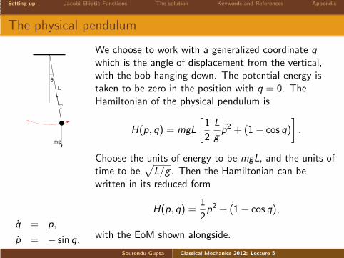
The physical pendulum

mg

L

T

θ

q = p,

p = − sin q.

We choose to work with a generalized coordinate q

which is the angle of displacement from the vertical,with the bob hanging down. The potential energy istaken to be zero in the position with q = 0. TheHamiltonian of the physical pendulum is

H(p, q) = mgL

[

1

2

L

gp2 + (1− cos q)

]

.

Choose the units of energy to be mgL, and the units oftime to be

√

L/g . Then the Hamiltonian can bewritten in its reduced form

H(p, q) =1

2p2 + (1− cos q),

with the EoM shown alongside.



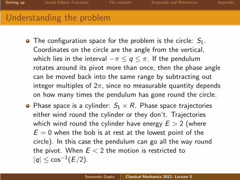
Understanding the problem

The configuration space for the problem is the circle: S1.Coordinates on the circle are the angle from the vertical,which lies in the interval −π ≤ q ≤ π. If the pendulumrotates around its pivot more than once, then the phase anglecan be moved back into the same range by subtracting outinteger multiples of 2π, since no measurable quantity dependson how many times the pendulum has gone round the circle.

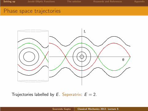
Phase space is a cylinder: S1 × R . Phase space trajectorieseither wind round the cylinder or they don’t. Trajectorieswhich wind round the cylinder have energy E > 2 (whereE = 0 when the bob is at rest at the lowest point of thecircle). In this case the pendulum can go all the way roundthe pivot. When E < 2 the motion is restricted to|q| ≤ cos−1(E/2).



Phase space trajectories

L

θ

Trajectories labelled by E . Seperatrix: E = 2.



Other examples

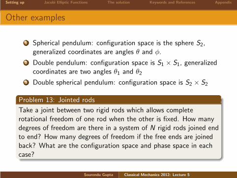
1 Spherical pendulum: configuration space is the sphere S2,generalized coordinates are angles θ and φ.

2 Double pendulum: configuration space is S1 × S1, generalizedcoordinates are two angles θ1 and θ2

3 Double spherical pendulum: configuration space is S2 × S2

Problem 13: Jointed rods

Take a joint between two rigid rods which allows completerotational freedom of one rod when the other is fixed. How manydegrees of freedom are there in a system of N rigid rods joined endto end? How many degrees of freedom if the free ends are joinedback? What are the configuration space and phase space in eachcase?



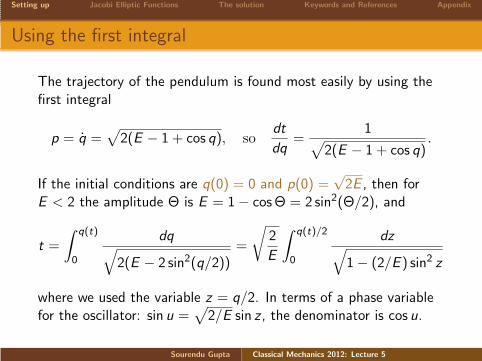
Using the first integral

The trajectory of the pendulum is found most easily by using thefirst integral

p = q =√

2(E − 1 + cos q), sodt

dq=

1√

2(E − 1 + cos q).

If the initial conditions are q(0) = 0 and p(0) =√2E , then for

E < 2 the amplitude Θ is E = 1− cosΘ = 2 sin2(Θ/2), and

t =

∫ q(t)

0

dq√

2(E − 2 sin2(q/2))=

√

2

E

∫ q(t)/2

0

dz√

1− (2/E ) sin2 z

where we used the variable z = q/2. In terms of a phase variablefor the oscillator: sin u =

√

2/E sin z , the denominator is cos u.



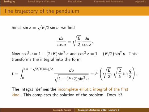
The trajectory of the pendulum

Since sin z =√

E/2 sin u, we find

dz

cos u=

√

E

2

du

cos z.

Now cos2 u = 1− (2/E ) sin2 z and cos2 z = 1− (E/2) sin2 u. Thistransforms the integral into the form

t =

∫ sin−1√

2/E sin q/2

0

du√

1− (E/2) sin2 u= F

(

√

E

2,

√

2

Esin

q

2

)

.

The integral defines the incomplete elliptic integral of the firstkind. This completes the solution of the problem. Does it?



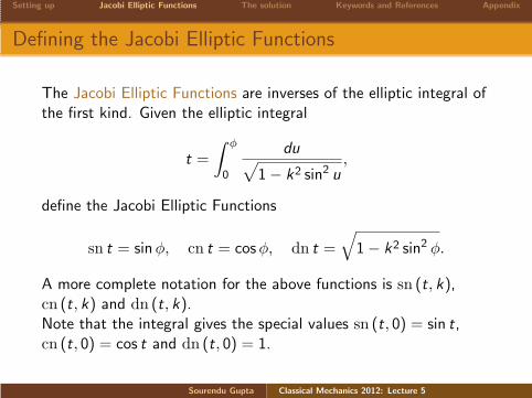
Defining the Jacobi Elliptic Functions

The Jacobi Elliptic Functions are inverses of the elliptic integral ofthe first kind. Given the elliptic integral

t =

∫ φ

0

du√

1− k2 sin2 u,

define the Jacobi Elliptic Functions

sn t = sinφ, cn t = cosφ, dn t =

√

1− k2 sin2 φ.

A more complete notation for the above functions is sn (t, k),cn (t, k) and dn (t, k).Note that the integral gives the special values sn (t, 0) = sin t,cn (t, 0) = cos t and dn (t, 0) = 1.



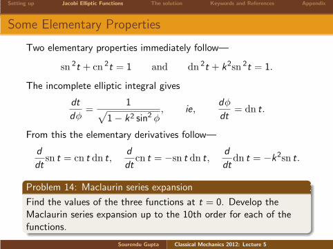
Some Elementary Properties

Two elementary properties immediately follow—

sn2t + cn

2t = 1 and dn2t + k2sn 2t = 1.

The incomplete elliptic integral gives

dt

dφ=

1√

1− k2 sin2 φ, ie,

dφ

dt= dn t.

From this the elementary derivatives follow—

d

dtsn t = cn t dn t,

d

dtcn t = −sn t dn t,

d

dtdn t = −k2sn t.

Problem 14: Maclaurin series expansion

Find the values of the three functions at t = 0. Develop theMaclaurin series expansion up to the 10th order for each of thefunctions.



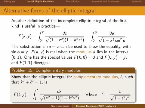
Alternative forms of the elliptic integral

Another definition of the incomplete elliptic integral of the firstkind is useful in practice—

F (k , y) =

∫ y

0

dz√

(1− z2)(1− k2z2)=

∫ φ

0

du√

1− k2 sin2 u.

The substitution sin u = z can be used to show the equality, withsinφ = y . F (k , y) is real when the modulus k lies in the interval(0, 1). One has the special values F (k , 0) = 0 and F (0, y) = y ,and F (1, 1) diverges.

Problem 15: Complementary modulus

Show that the elliptic integral for complementary modulus, ℓ, suchthat k2 + ℓ2 = 1, is

F (ℓ, y) =

∫ f

1

dx√

(x2 − 1)(1− k2x2), where f =

1√

1− ℓ2y2.



Periodicity: the argument

In order to establish the periodicity of the Jacobi elliptic functions,it is enough to prove it for any one of the functions. We willchoose to prove it for sn .Why is a proof needed?A functional relation of the form f (t) = sinφ is not sufficient toshow that f (t) is periodic. Consider f ≡ tanh, for example. So aproof is needed.The idea of the proofIn order to prove periodicity, one needs to prove two things: (a)that t is finite for finite φ, (b) increasing φ by 2π should increase t

by a fixed amount, for every value of φ.For the counter-example above, the condition (a) failed.



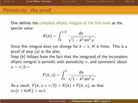
Periodicity: the proof

One defines the complete elliptic integral of the first kind as thespecial value

K (k) =

∫ π/2

0

du√

1− k2 sin2 u,

Since this integral does not diverge for k < 1, K is finite. This is aproof of step (a) in the plan.Step (b) follows from the fact that the integrand of the incompleteelliptic integral is periodic with periodicity π, and symmetric aboutu = π/2—

F (k , φ) =

∫ φ

0

du√

1− k2 sin2 u,

As a result, F (k , φ+ π/2) = K (k) + F (k , φ), so thatsn (t + 4nK ) = sn t.



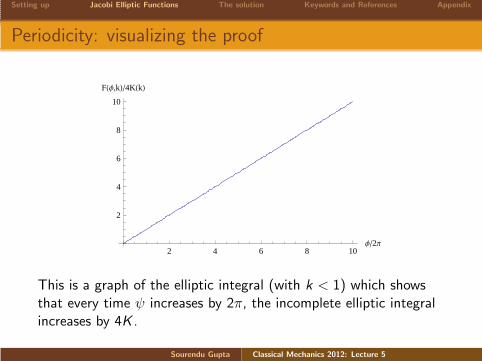
Periodicity: visualizing the proof

2 4 6 8 10Φ�2Π

2

4

6

8

10

FHΦ,kL�4KHkL

This is a graph of the elliptic integral (with k < 1) which showsthat every time ψ increases by 2π, the incomplete elliptic integralincreases by 4K .



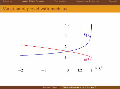
Variation of period with modulus



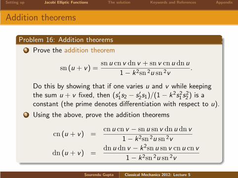
Addition theorems

Problem 16: Addition theorems

1 Prove the addition theorem

sn (u + v) =sn u cn v dn v + sn v cn u dn u

1− k2sn 2u sn 2v.

Do this by showing that if one varies u and v while keepingthe sum u + v fixed, then (s ′1s2 − s ′2s1)/(1− k2s21 s

22 ) is a

constant (the prime denotes differentiation with respect to u).

2 Using the above, prove the addition theorems

cn (u + v) =cn u cn v − sn u sn v dn u dn v

1− k2sn 2u sn 2v

dn (u + v) =dn u dn v − k2sn u sn v cn u cn v

1− k2sn 2u sn 2v



Special values and periodicity

From the integral representation one find

snK = 1, cnK = 0 and dnK = ℓ.

Then, using the addition theorems, one finds

sn 2K = 0, cn 2K = −1 and dn 2K = 1.

Further use of the addition theorems gives

sn 3K = −1, cn 3K = 0 and dn 3K = ℓ.

Problem 17: Quarter and half period identities

Express the Jacobi elliptic functions for values of arguments t ± K ,t ± 2K and t ± 3K in terms of the functions evaluated at t.



Complex periodicity

Introduce the notation for the complete elliptic integral of thecomplementary modulus, K (ℓ) = K ′. Then, from the expressionsderived earlier, we can write

L = K + iK ′ =

∫ 1/k

0

dz√

(1− z2)(1− k2z2).

This implies that sn L = 1/k and dn L = 0, whereas cn L = −iℓ/k .By using the addition theorems we have sn 2L = 0, cn 2L = 1 anddn 2L = −1. Further, sn 4L = 0, cn 4L = 1 and dn 4L = 1.As a result, we have the complex periodicity relations

sn (t + 4L) =sn t cn 4L dn 4L+ sn 4L cn t dn t

1− k2sn 2t sn 24L= sn t,

cn (t + 4L) = = cn t, and dn (t + 4L) = dn t.

Utilizing the periodicity in 4K , we find that the functions haveperiodicity of 4iK ′.



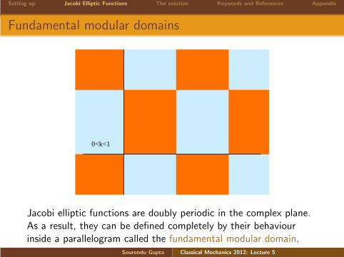
Fundamental modular domains

0<k<1

Jacobi elliptic functions are doubly periodic in the complex plane.As a result, they can be defined completely by their behaviourinside a parallelogram called the fundamental modular domain.



Poles

Using the addition theorem we can write

sn (t + iK ′) = sn (t + L− K ) =cn (t + L)dn (t + L)

1− k2sn 2(t + L).

Again, using the addition theorem we have,

sn (t + L) =cn t dn t

k(1− sn 2t)=

dn t

kcn t

cn (t + L) = − iℓcn t

k(1− sn 2t)= − iℓ

kcn t

dn (t + L) =iℓsn t cn t

1− sn 2t=

iℓsn t

cn t.

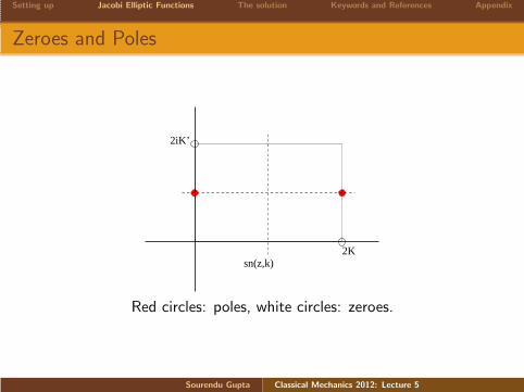
Putting these together, we find sn (t + iK ′) = 1/sn t. Since theTaylor expansion gives sn t = t +O(t3), sn has a simple pole atiK ′. As a result, cn and dn also have simple poles at the samepoint. By the periodicity relations, there is also a pole at 2K + iK ′.



Zeroes and Poles

sn(z,k)2K

2iK’

Red circles: poles, white circles: zeroes.



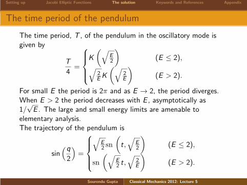
The time period of the pendulum

The time period, T , of the pendulum in the oscillatory mode isgiven by

T

4=

K

(

√

E2

)

(E ≤ 2),√

2EK

(

√

2E

)

(E > 2).

For small E the period is 2π and as E → 2, the period diverges.When E > 2 the period decreases with E , asymptotically as1/√E . The large and small energy limits are amenable to

elementary analysis.The trajectory of the pendulum is

sin(q

2

)

=

√

E2 sn

(

t,√

E2

)

(E ≤ 2),

sn

(

√

E2 t,√

2E

)

(E > 2).



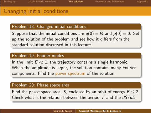
Changing initial conditions

Problem 18: Changed initial conditions

Suppose that the initial conditions are q(0) = Θ and p(0) = 0. Setup the solution of the problem and see how it differs from thestandard solution discussed in this lecture.

Problem 19: Fourier modes

In the limit E ≪ 1, the trajectory contains a single harmonic.When the amplitude is larger, the solution contains many Fouriercomponents. Find the power spectrum of the solution.

Problem 20: Phase space area

Find the phase space area, S , enclosed by an orbit of energy E ≤ 2.Check what is the relation between the period T and the dS/dE .



Keywords and References

Keywords

seperatrix, period, incomplete elliptic integral of the first kind,complete elliptic integral of the first kind, Jacobi elliptic functions,modulus, complementary modulus, fundamental modular domain,poles and zeroes

References

Whittaker and Watson, Chapter XXII.



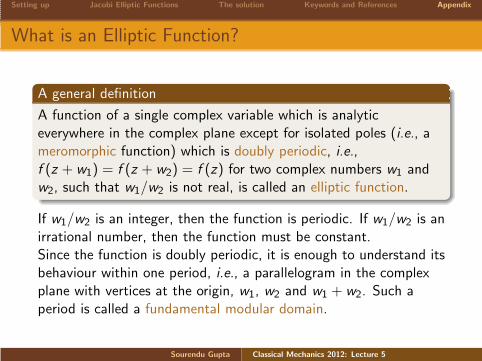
What is an Elliptic Function?

A general definition

A function of a single complex variable which is analyticeverywhere in the complex plane except for isolated poles (i.e., ameromorphic function) which is doubly periodic, i.e.,f (z + w1) = f (z + w2) = f (z) for two complex numbers w1 andw2, such that w1/w2 is not real, is called an elliptic function.

If w1/w2 is an integer, then the function is periodic. If w1/w2 is anirrational number, then the function must be constant.Since the function is doubly periodic, it is enough to understand itsbehaviour within one period, i.e., a parallelogram in the complexplane with vertices at the origin, w1, w2 and w1 + w2. Such aperiod is called a fundamental modular domain.



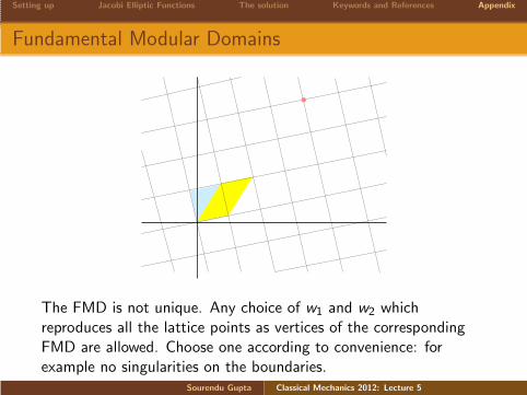
Fundamental Modular Domains

The FMD is not unique. Any choice of w1 and w2 whichreproduces all the lattice points as vertices of the correspondingFMD are allowed. Choose one according to convenience: forexample no singularities on the boundaries.



Analytic properties

The following theorems give fundamental properties of the ellipticfunctions:

1 The number of poles in any FMD is finite: otherwise alimit point would exist, which would be an essential singularityof the function.

2 The number of zeroes in any FMD is finite: otherwisethere would be an essential singularity of the reciprocal of thefunction.

3 The sum over residues in any FMD vanishes: provenchoosing an FMD which contains no poles on the boundariesand then using periodicity along with the Cauchy theorem.

4 An elliptic function without poles is constant: a specialcase of a more general theorem on meromorphic functions.



The order of an elliptic function

Defining the order

The order of an elliptic function f (z) is the number of roots off (z) = c within one fundamental modular domain.

The Cauchy theorem can be used to show that the number ofzeroes of the above equation is equal to the number of poles.Since every pole of f (z)− c is also a pole of f (z), the definition ofthe order does not depend on c .The order of an elliptic function must be at least 2, otherwise thesum over residues cannot vanish.The Jacobi elliptic functions are of order 2 and consist of twosimple poles in each FMD. The Weierstrass elliptic functions arealso of order 2 and contain an irreducible double pole. These arethe only elliptic functions of order 2.


The Physical Pendulum - Tata Institute of Fundamental...

Documents

Transcript of The Physical Pendulum - Tata Institute of Fundamental...