The physical characterisation of polysaccharides in solution
77
The physical characterisation of polysaccharides in solution Stephen Harding University of Nottingham
Transcript of The physical characterisation of polysaccharides in solution
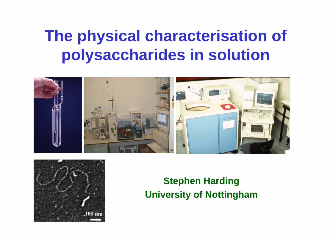
The physical characterisation of polysaccharides in solution
Stephen HardingUniversity of Nottingham
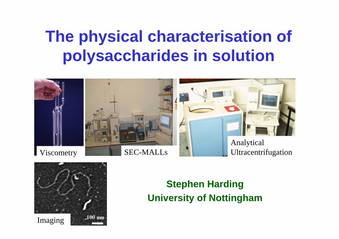
Viscometry SEC-MALLsAnalytical Ultracentrifugation
Imaging
The physical characterisation of polysaccharides in solution
Stephen HardingUniversity of Nottingham

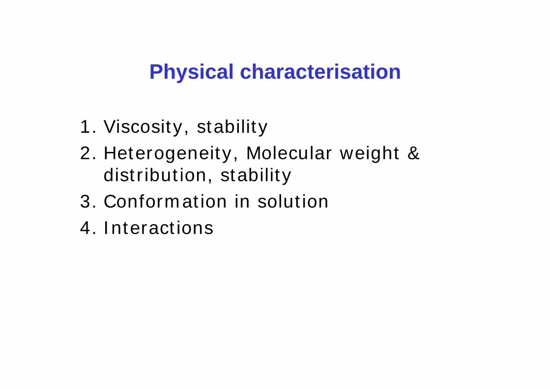
Physical characterisation
1. Viscosity, stability2. Heterogeneity, Molecular weight &
distribution, stability3. Conformation in solution4. Interactions
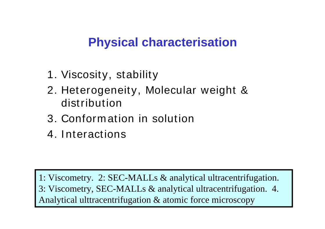
Physical characterisation
1. Viscosity, stability2. Heterogeneity, Molecular weight &
distribution3. Conformation in solution4. Interactions
1: Viscometry. 2: SEC-MALLs & analytical ultracentrifugation. 3: Viscometry, SEC-MALLs & analytical ultracentrifugation. 4. Analytical ulttracentrifugation & atomic force microscopy
1. Viscosity from precision viscometry
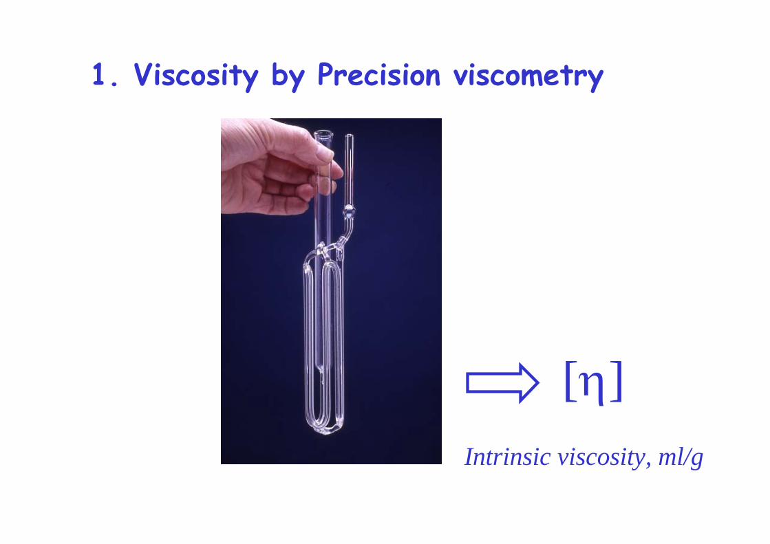
1. Viscosity by Precision viscometry
[η]Intrinsic viscosity, ml/g
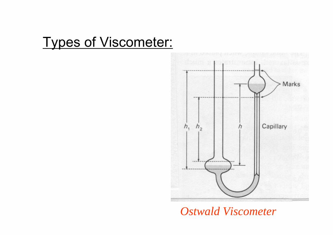
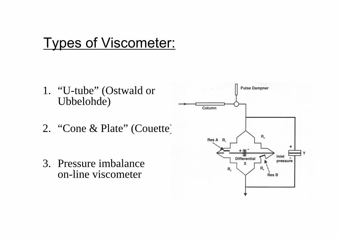
Types of Viscometer:
Ostwald Viscometer
1. “U-tube” (Ostwald or Ubbelohde)
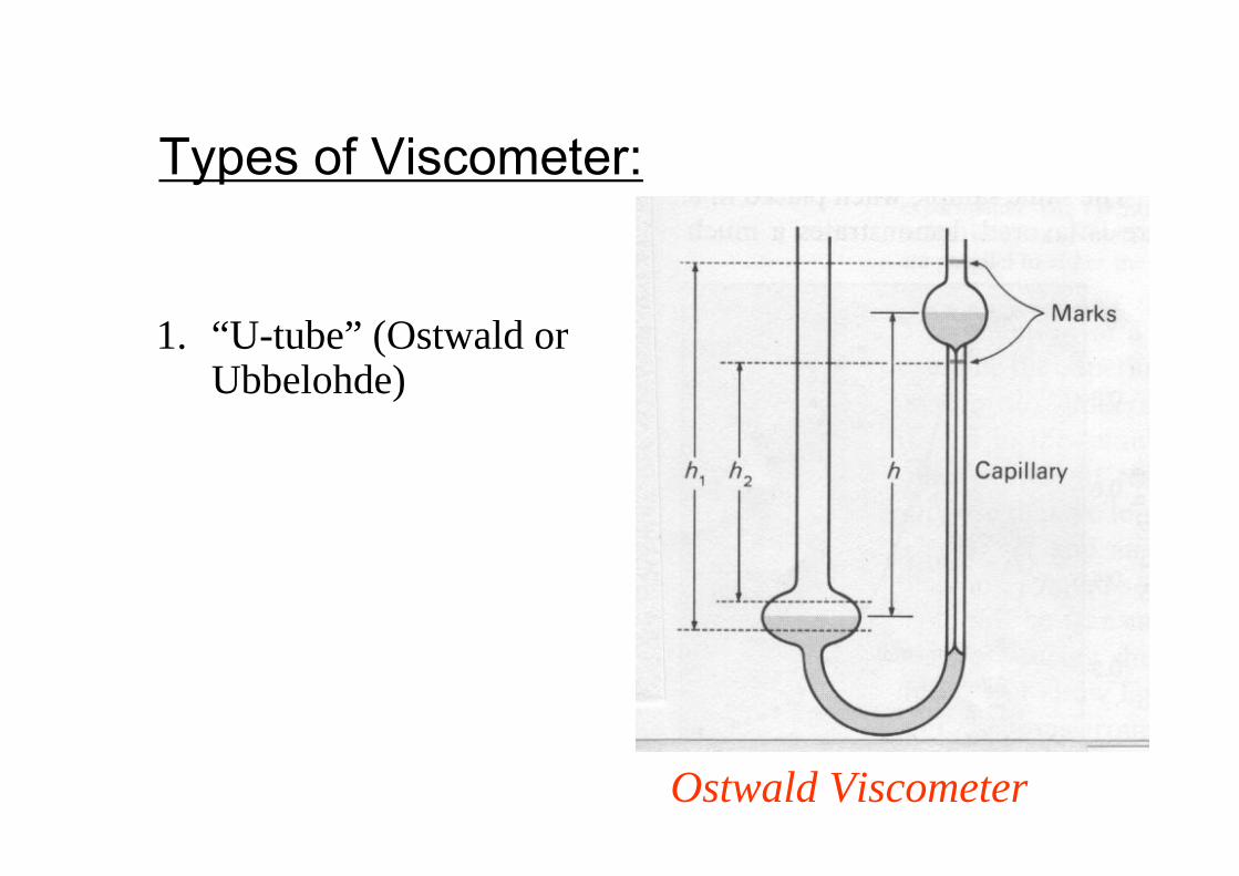
Types of Viscometer:
Ostwald Viscometer
1. “U-tube” (Ostwald or Ubbelohde)
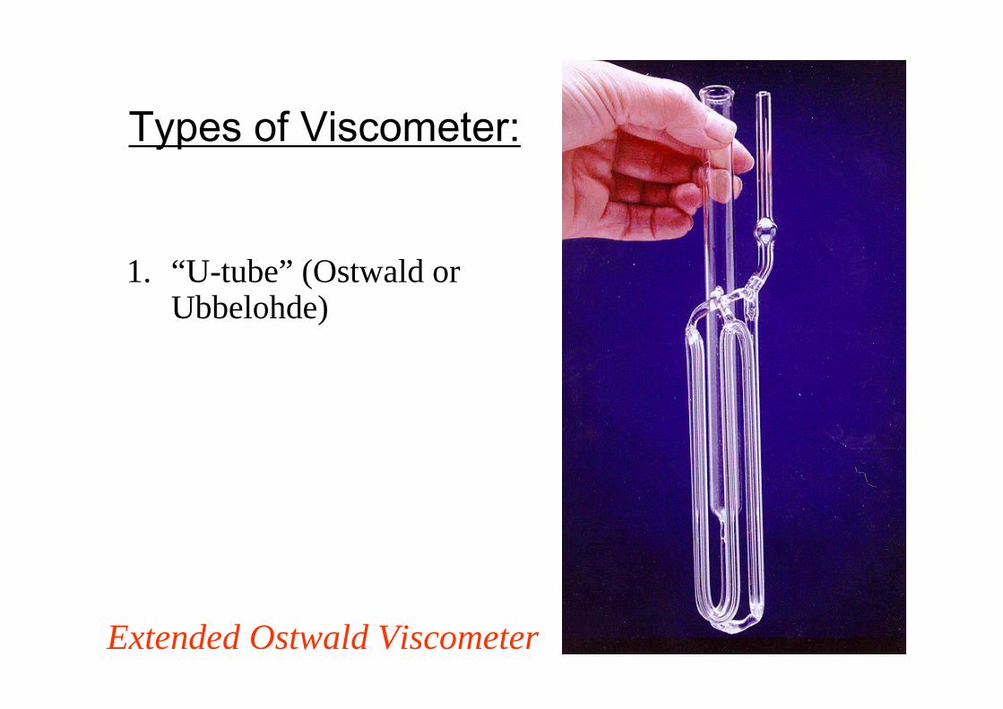
Types of Viscometer:
Extended Ostwald Viscometer
1. “U-tube” (Ostwald or Ubbelohde)
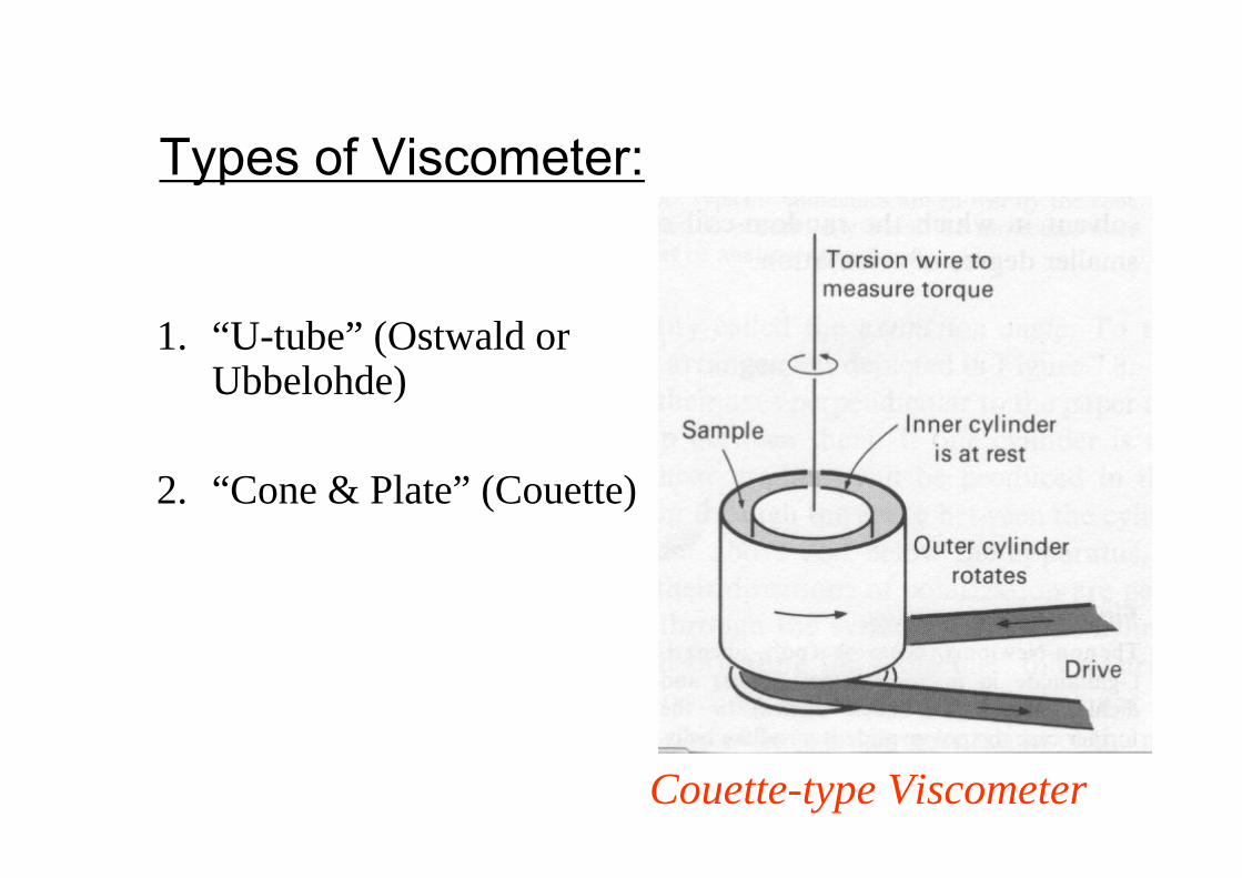
2. “Cone & Plate” (Couette)
Types of Viscometer:
Couette-type Viscometer
1. “U-tube” (Ostwald or Ubbelohde)
2. “Cone & Plate” (Couette)
3. Pressure imbalance on-line viscometer
Types of Viscometer:
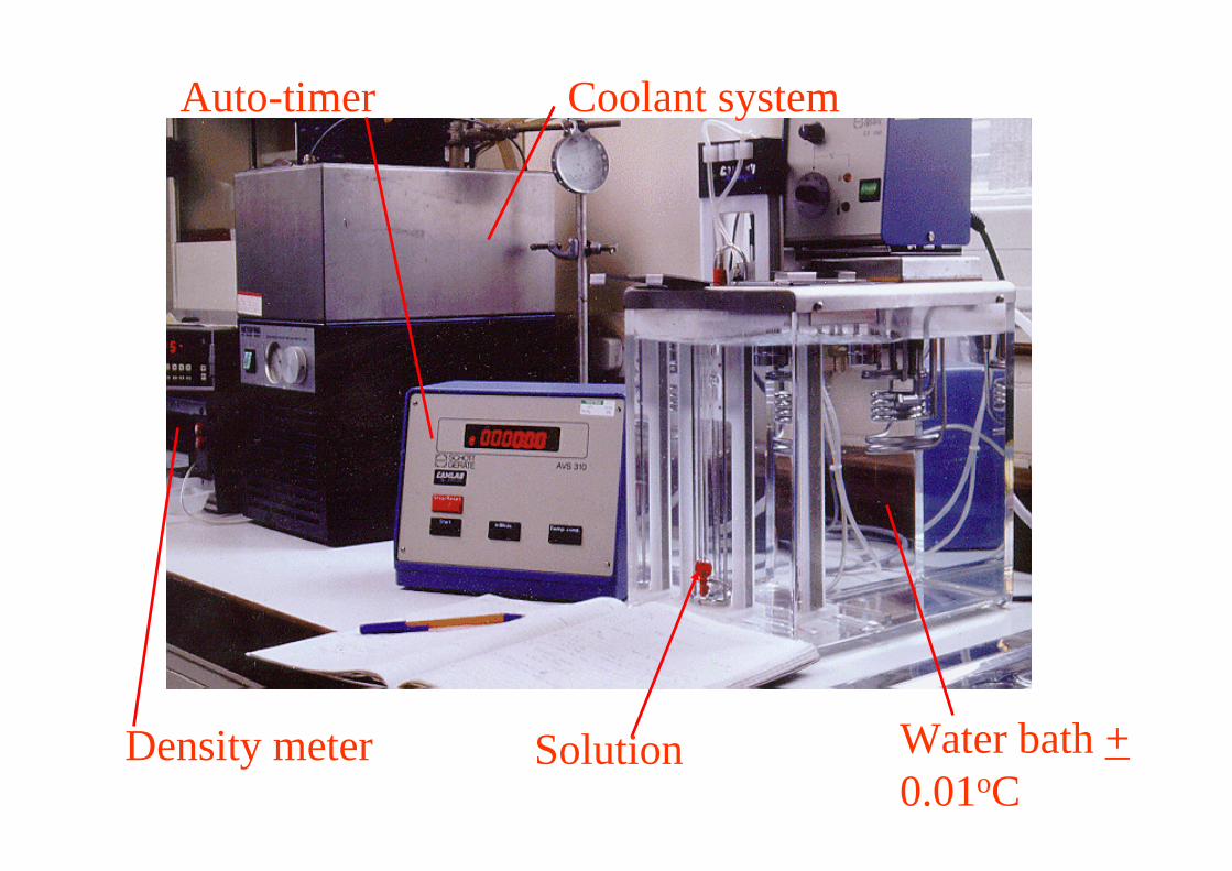
Water bath +0.01oC
Density meter
Coolant system
Solution
Auto-timer
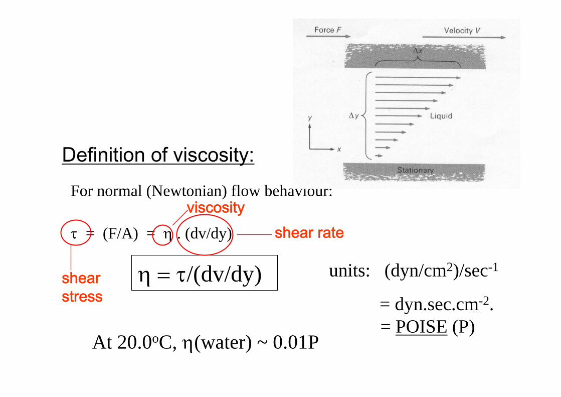
For normal (Newtonian) flow behaviour:
τ = (F/A) = η . (dv/dy)
Definition of viscosity:
η = τ/(dv/dy) units: (dyn/cm2)/sec-1
= dyn.sec.cm-2. . = POISE (P)
At 20.0oC, η(water) ~ 0.01P
shear stress
shear rateviscosity
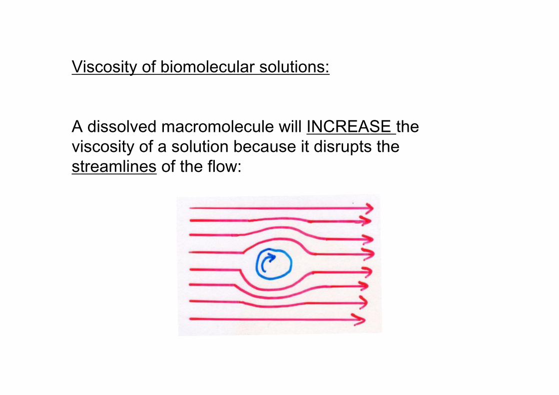
Viscosity of biomolecular solutions:
A dissolved macromolecule will INCREASE the viscosity of a solution because it disrupts the streamlines of the flow:
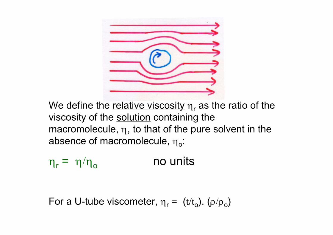
We define the relative viscosity ηr as the ratio of the viscosity of the solution containing the macromolecule, η, to that of the pure solvent in the absence of macromolecule, ηo:
ηr = η/ηo no units
For a U-tube viscometer, ηr = (t/to). (ρ/ρo)
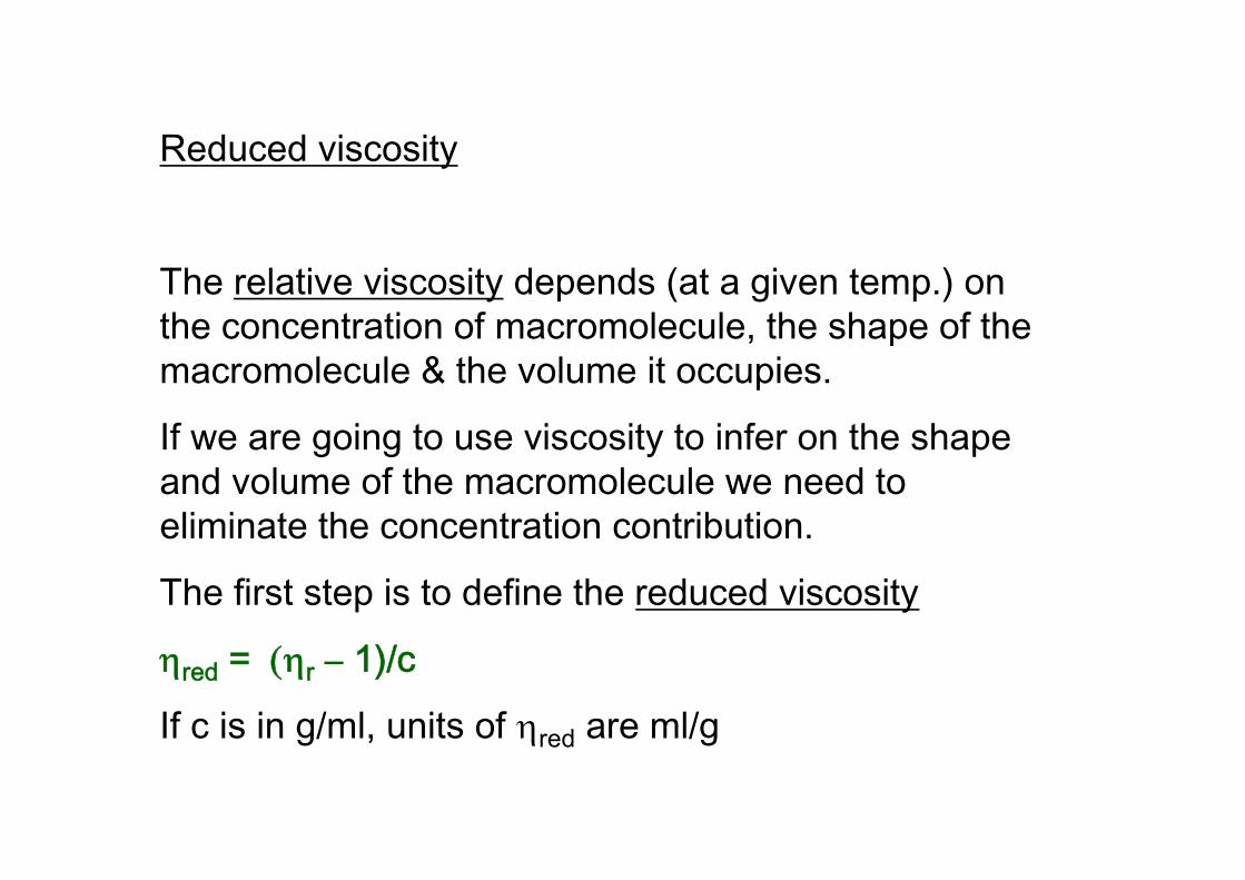
Reduced viscosity
The relative viscosity depends (at a given temp.) on the concentration of macromolecule, the shape of the macromolecule & the volume it occupies.
If we are going to use viscosity to infer on the shape and volume of the macromolecule we need to eliminate the concentration contribution.
The first step is to define the reduced viscosity
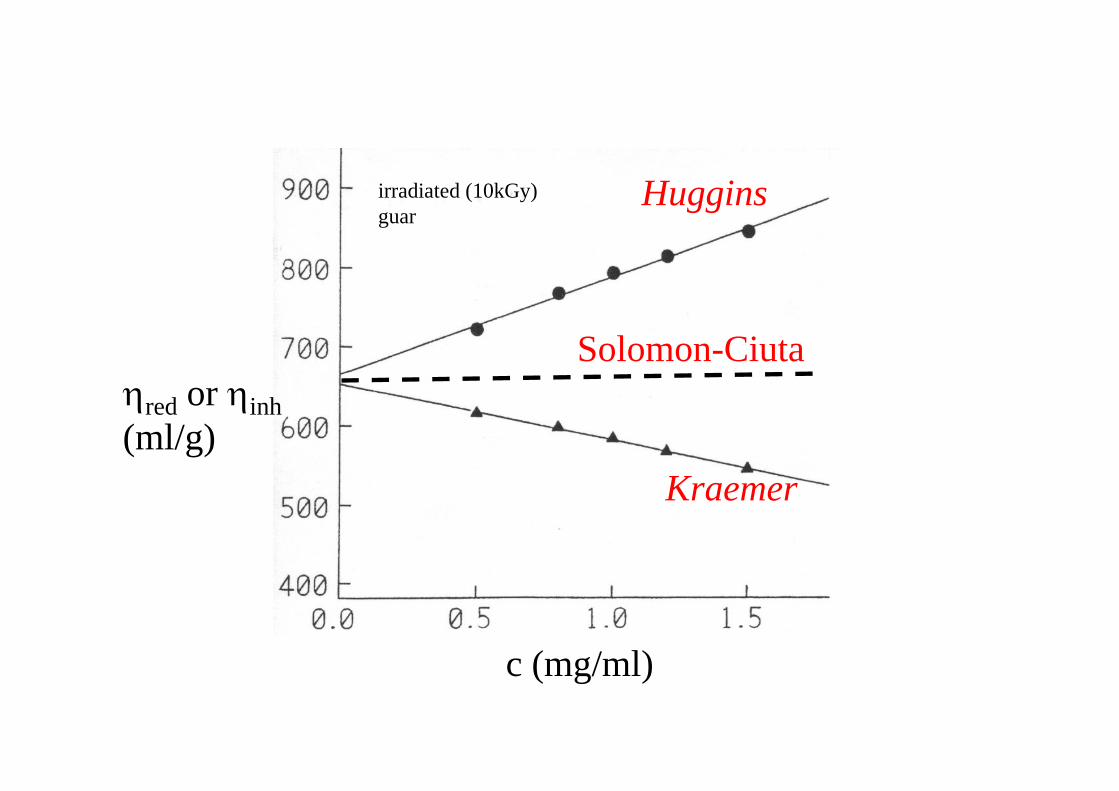
ηred = (ηr – 1)/c
If c is in g/ml, units of ηred are ml/g
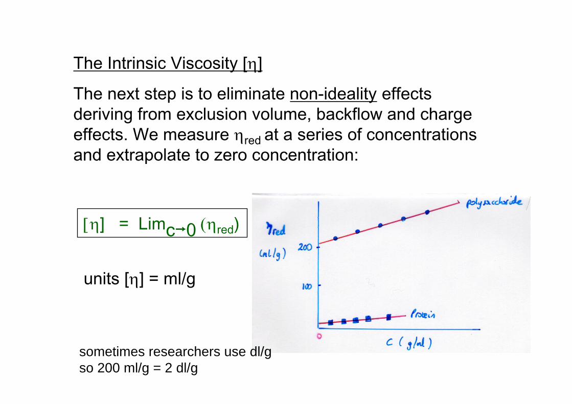
The Intrinsic Viscosity [η]
The next step is to eliminate non-ideality effects deriving from exclusion volume, backflow and charge effects. We measure ηred at a series of concentrations and extrapolate to zero concentration:
[η] = Limc⃗0 (ηred)
units [η] = ml/g
sometimes researchers use dl/gso 200 ml/g = 2 dl/g
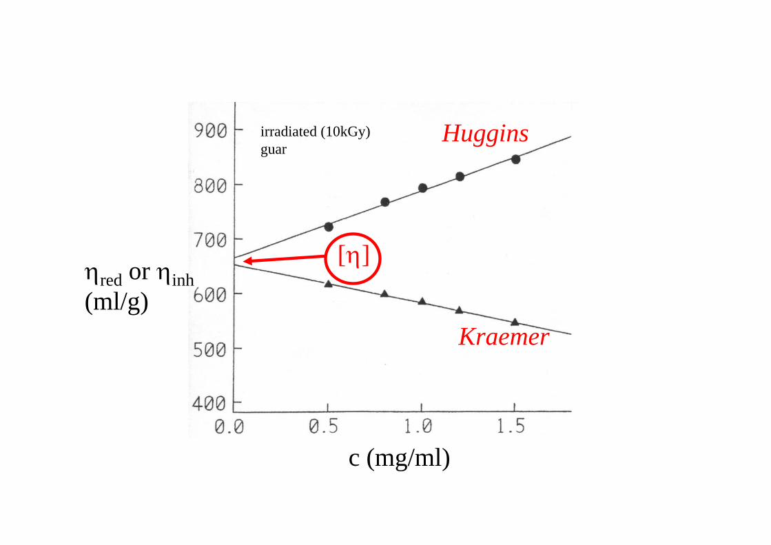
c (mg/ml)
Kraemer
Huggins
[η]ηred or ηinh(ml/g)
irradiated (10kGy) guar
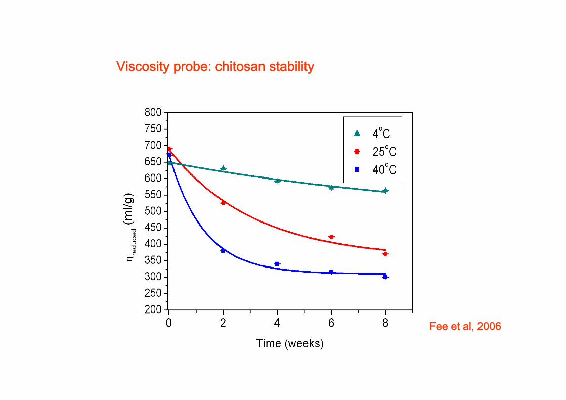
Viscosity probe: chitosan stability
Fee et al, 2006
2. Heterogeneity and molecular weight: SEC-MALLs
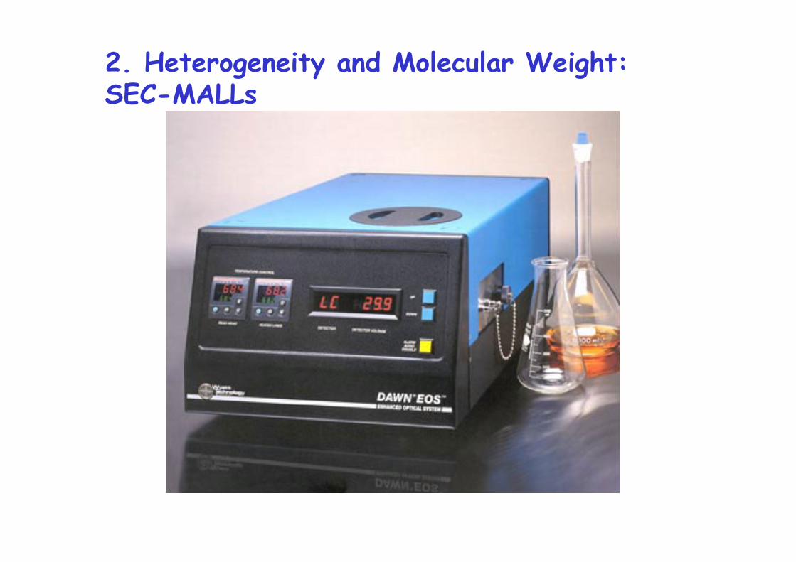
2. Heterogeneity and Molecular Weight: SEC-MALLs
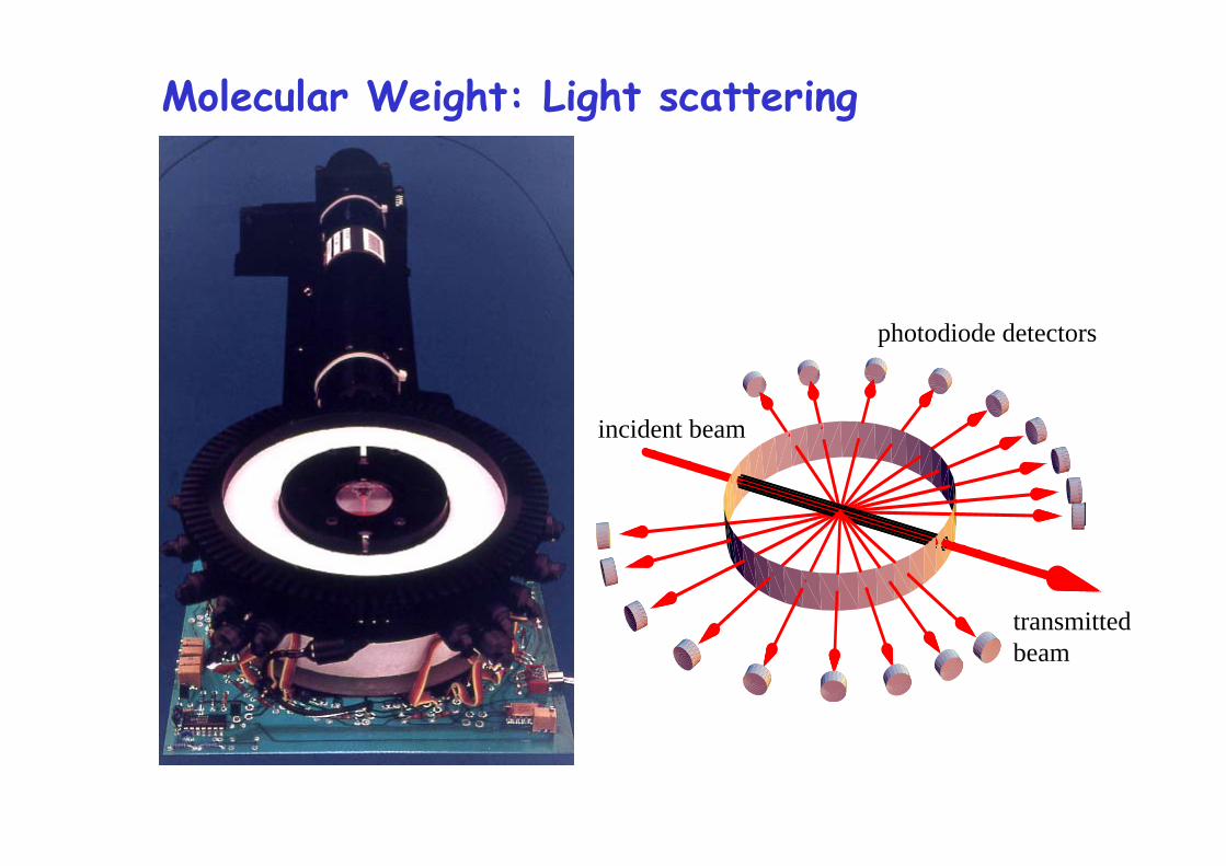
Molecular Weight: Light scattering
transmittedbeam
photodiode detectors
incident beam
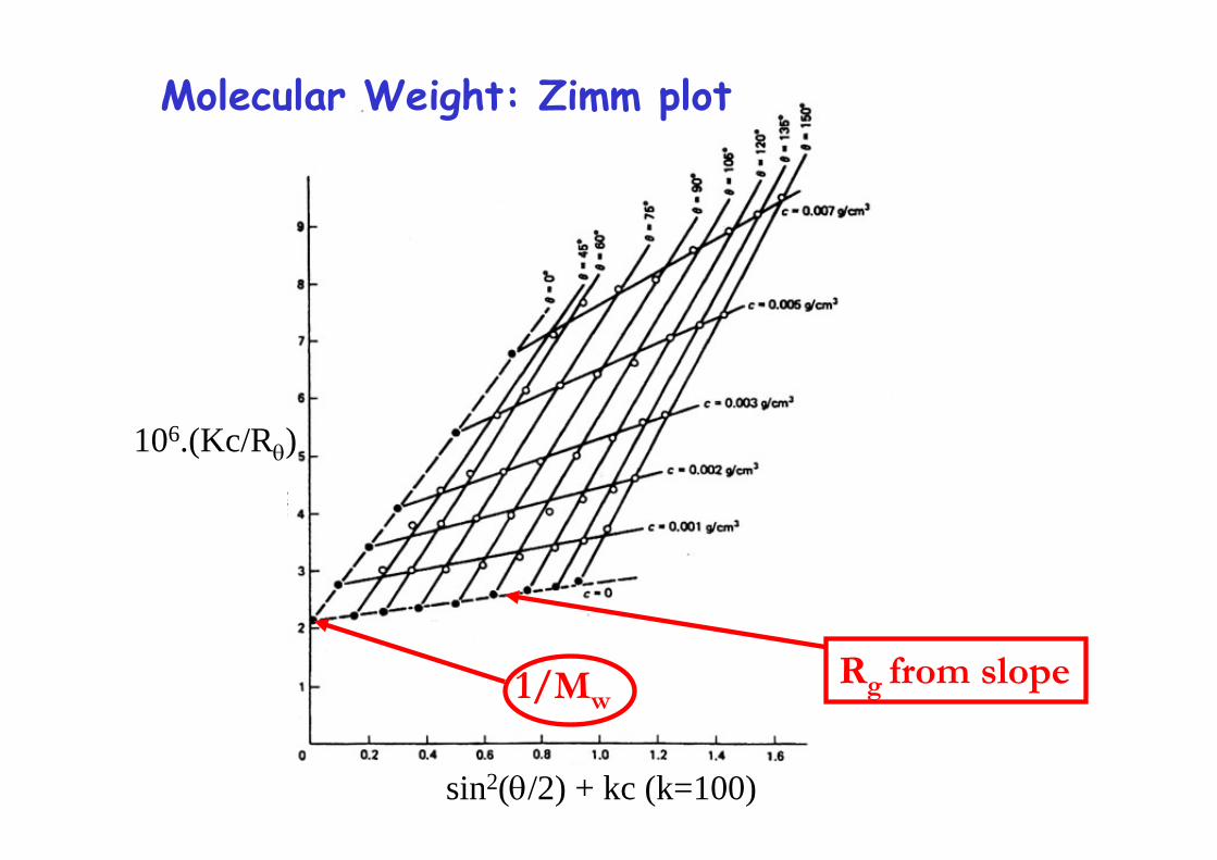
Molecular Weight: Zimm plot
1/Mw
sin2(θ/2) + kc (k=100)
106.(Kc/Rθ)
Rg from slope
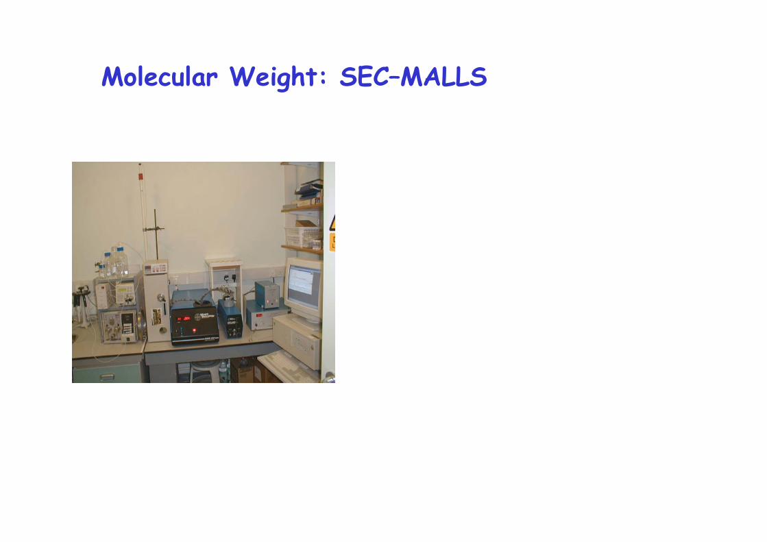
Molecular Weight: SEC–MALLS
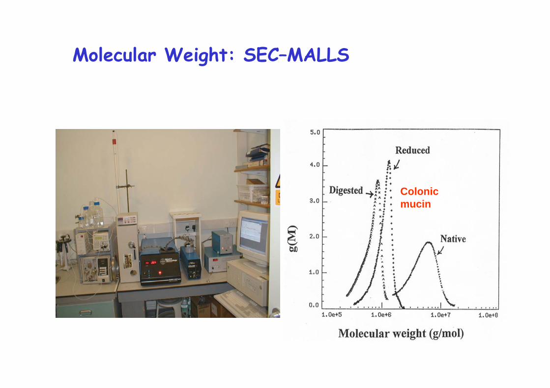
Molecular Weight: SEC–MALLS
Colonic mucin
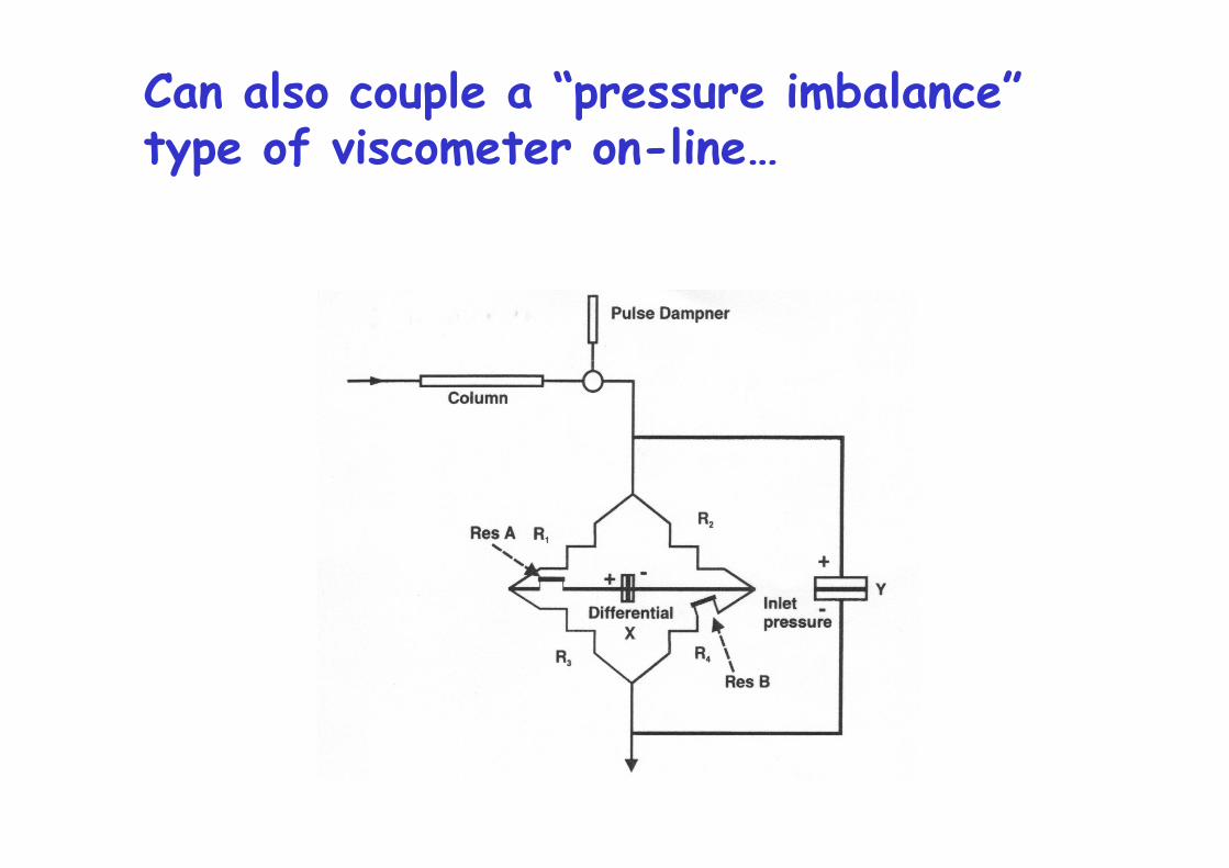
Can also couple a “pressure imbalance”type of viscometer on-line…

c (mg/ml)
Kraemer
Huggins
[η]ηred or ηinh(ml/g)
irradiated (10kGy) guar
c (mg/ml)
Kraemer
Huggins
Solomon-Ciutaηred or ηinh(ml/g)
irradiated (10kGy) guar
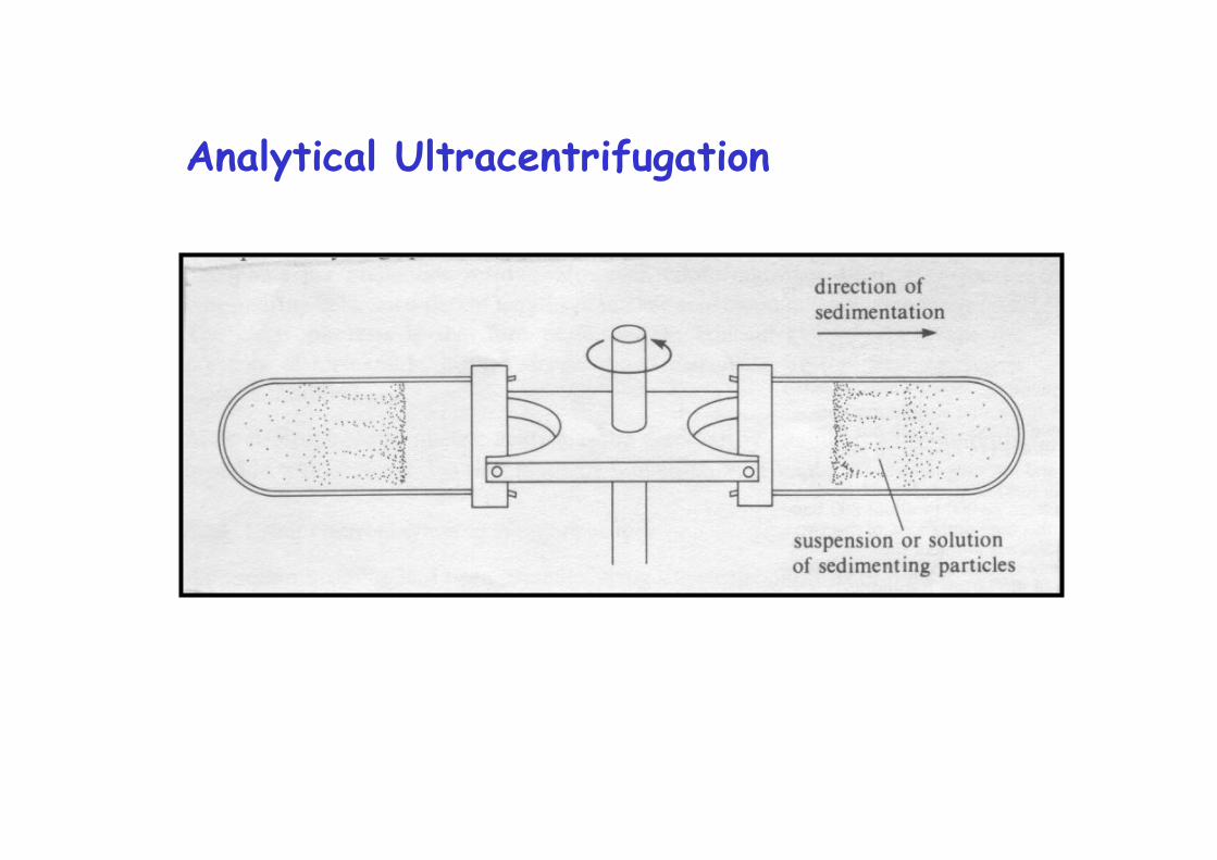
Analytical Ultracentrifugation
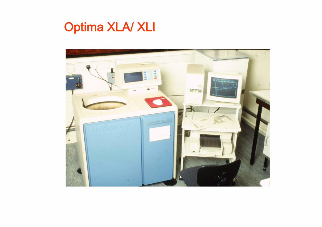
Optima XLA/ XLI
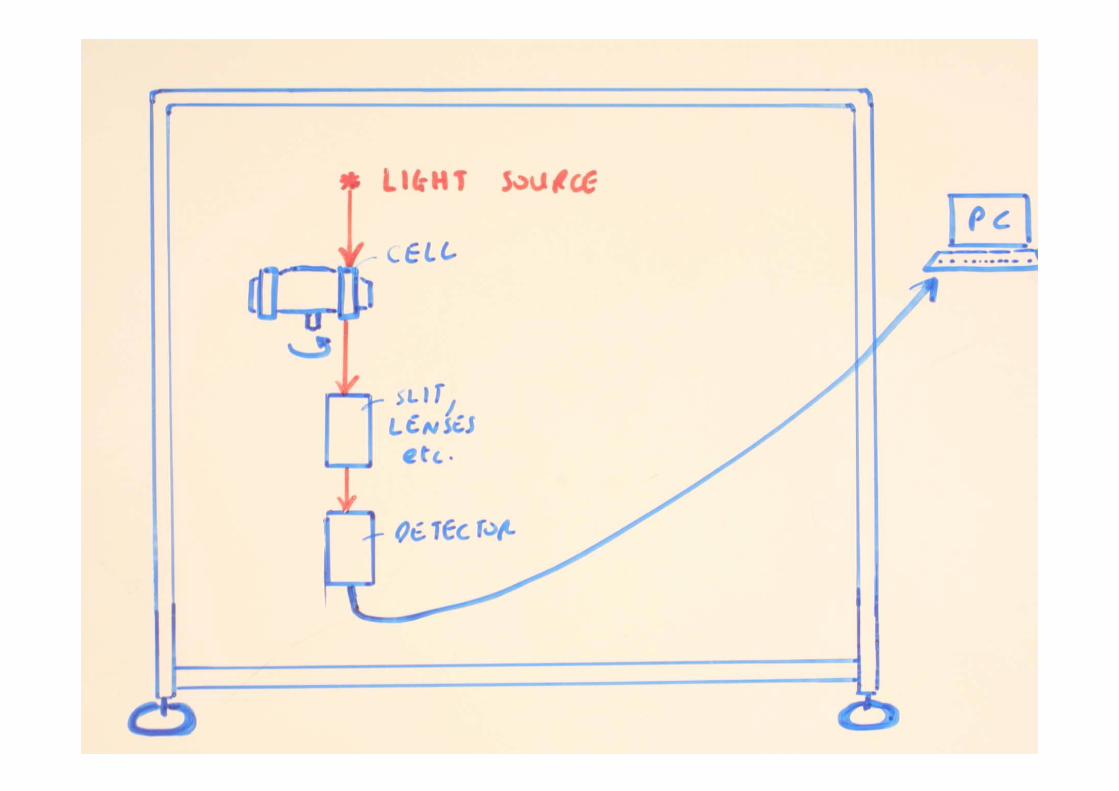

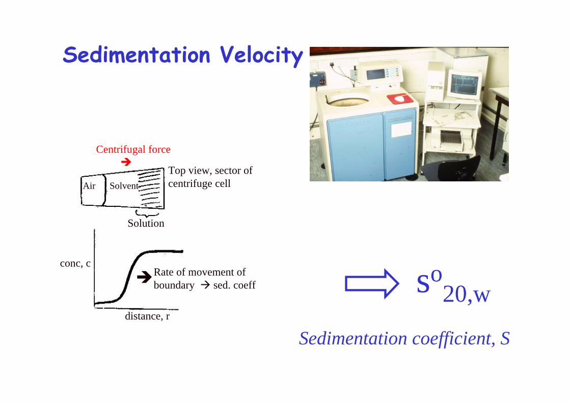
Sedimentation Velocity
Air Solvent
Solution
conc, c
distance, r
Top view, sector ofcentrifuge cell
Rate of movement ofboundary sed. coeff
Centrifugal force
so20,w
Sedimentation coefficient, S
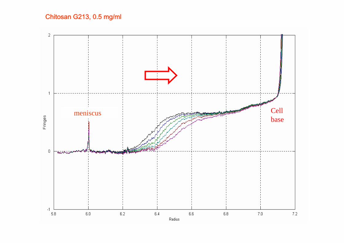
Chitosan G213, 0.5 mg/ml
meniscus Cell base
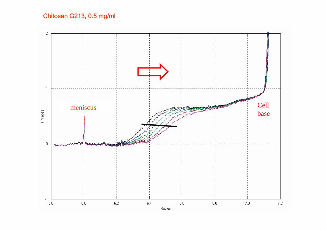
Chitosan G213, 0.5 mg/ml
meniscus Cell base
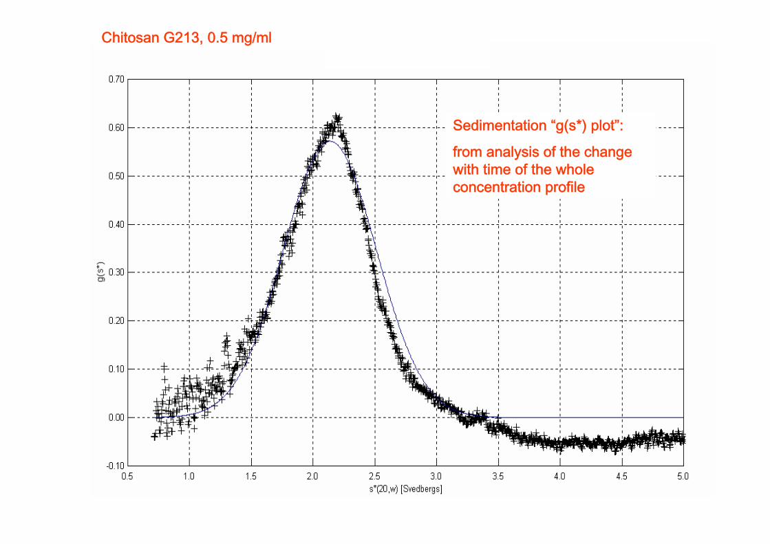
Chitosan G213, 0.5 mg/ml
Sedimentation “g(s*) plot”:
from analysis of the change with time of the whole concentration profile
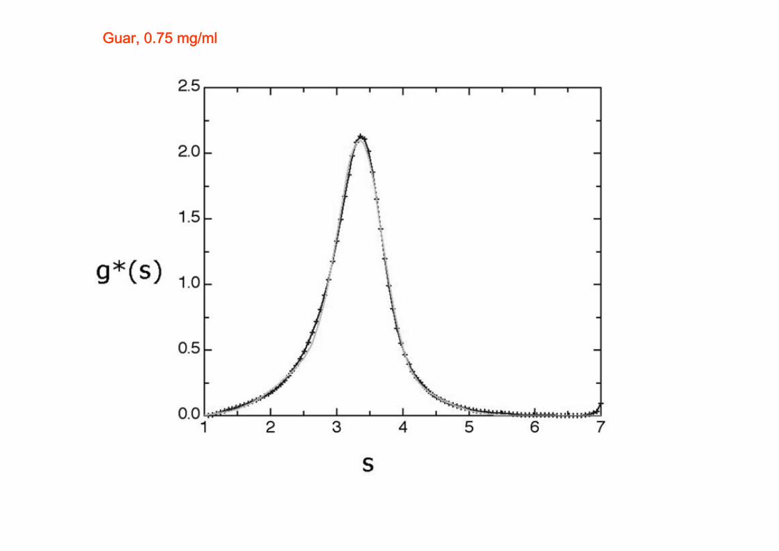
Guar, 0.75 mg/ml
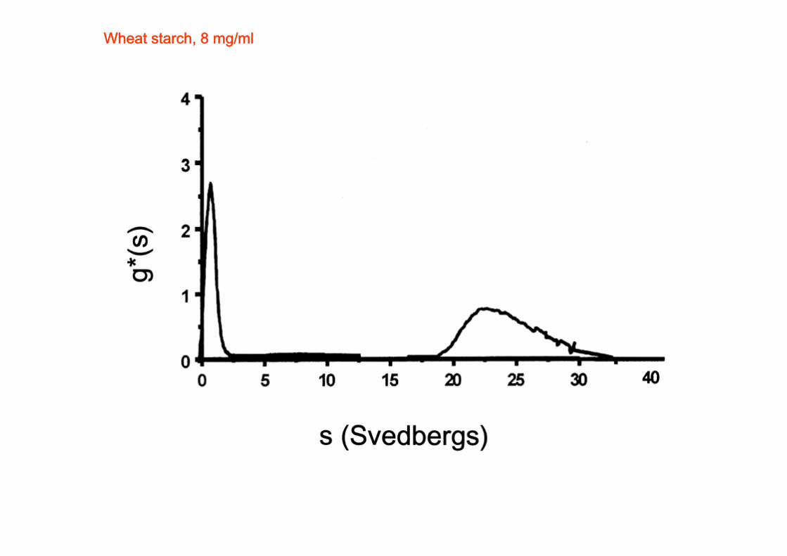
Wheat starch, 8 mg/ml
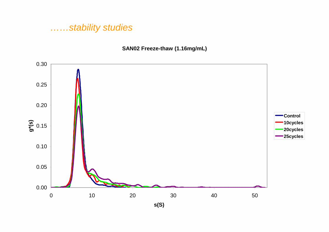
SAN02 Freeze-thaw (1.16mg/mL)
0.00
0.05
0.10
0.15
0.20
0.25
0.30
0 10 20 30 40 50
s(S)
g*(s
)
Control10cycles20cycles25cycles
……stability studies
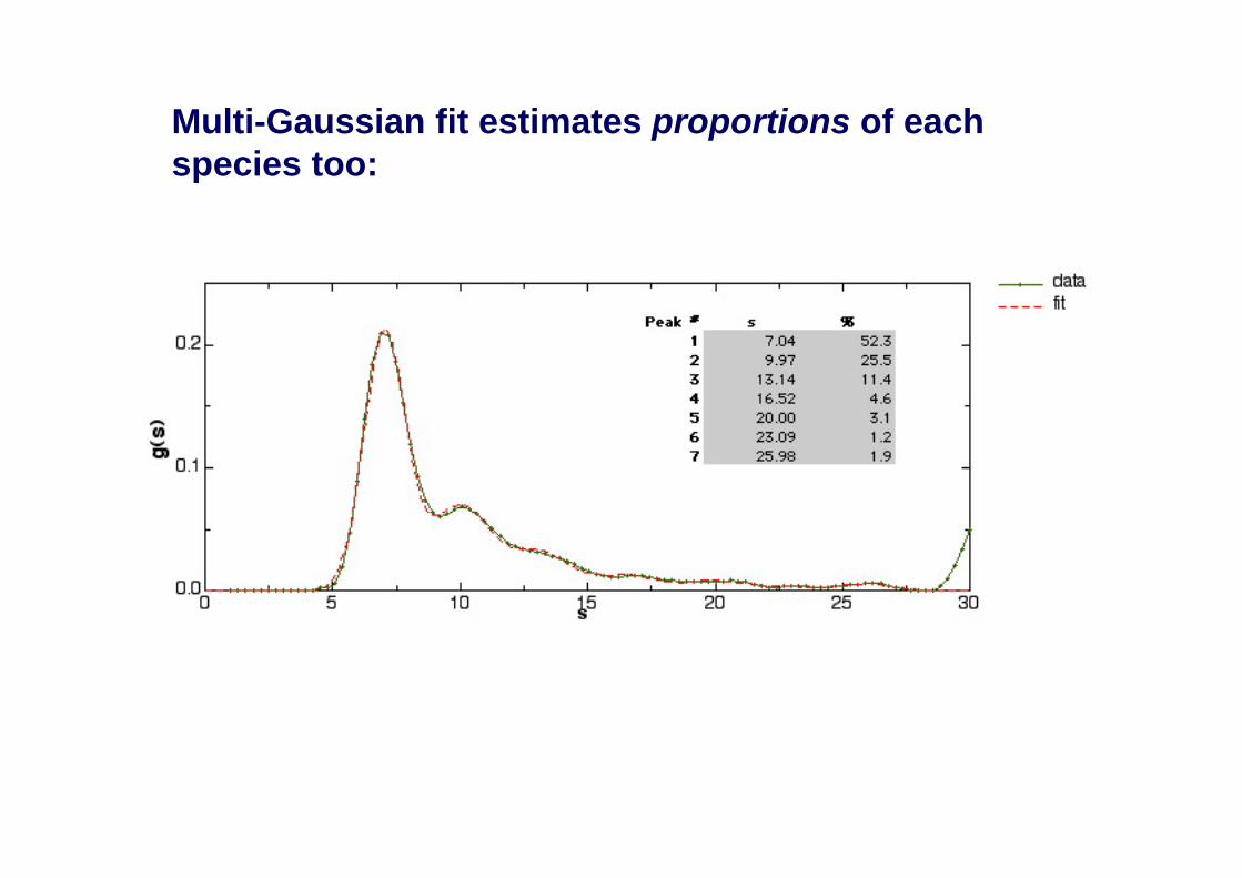
Multi-Gaussian fit estimates proportions of each species too:
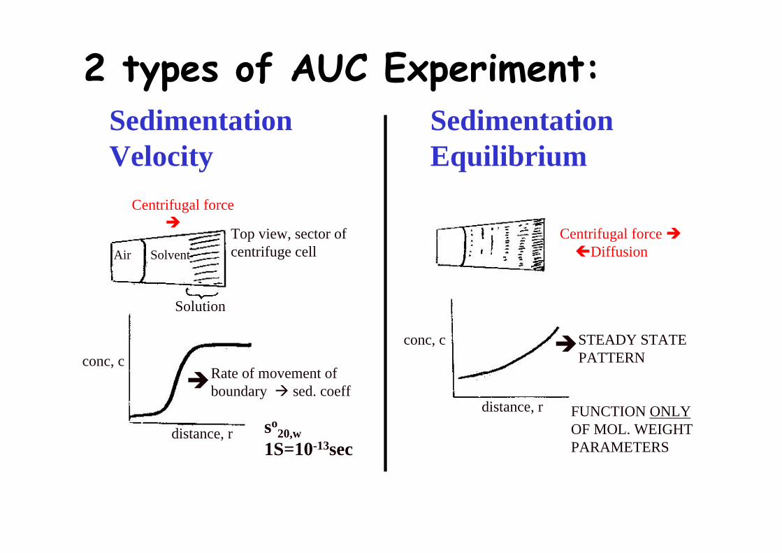
Sedimentation Velocity
Sedimentation Equilibrium
2 types of AUC Experiment:
Air Solvent
Solution
conc, c
distance, r
Top view, sector ofcentrifuge cell
Rate of movement ofboundary sed. coeff
Centrifugal force
conc, c STEADY STATEPATTERN
FUNCTION ONLY OF MOL. WEIGHT PARAMETERS
distance, r
Centrifugal force Diffusion
so20,w
1S=10-13sec
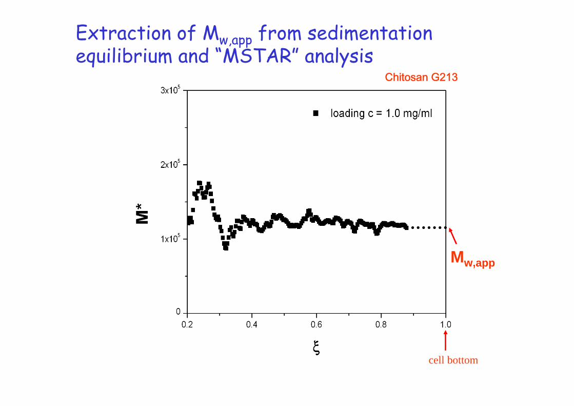
Mw,app
cell bottom
Extraction of Mw,app from sedimentation equilibrium and “MSTAR” analysis
Chitosan G213
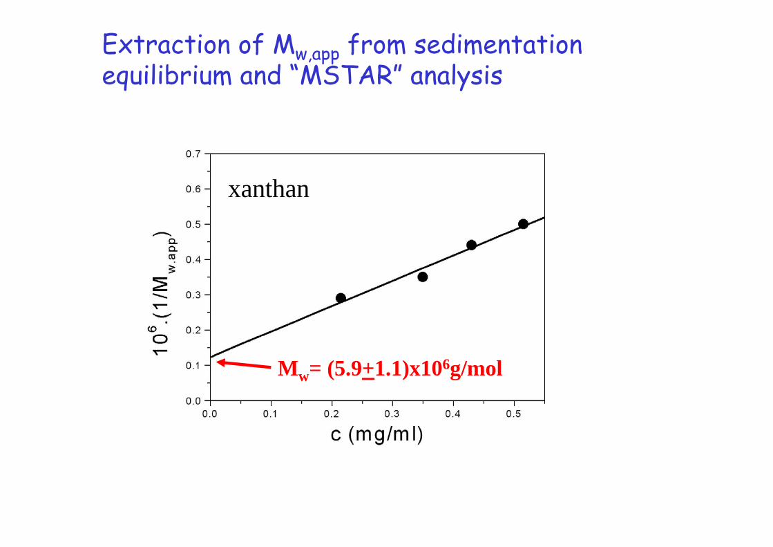
Extraction of Mw,app from sedimentation equilibrium and “MSTAR” analysis
Mw= (5.9+1.1)x106g/mol
xanthan

3. Conformation in solution
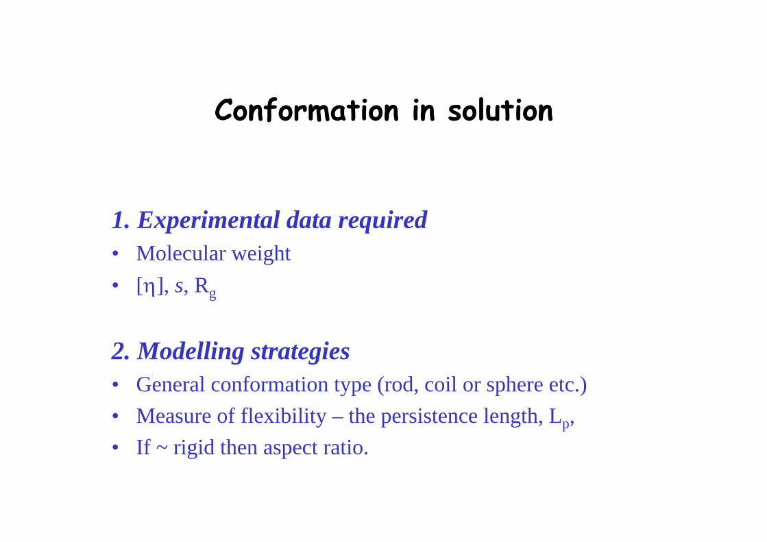
Conformation in solution
1. Experimental data required• Molecular weight• [η], s, Rg
2. Modelling strategies • General conformation type (rod, coil or sphere etc.)• Measure of flexibility – the persistence length, Lp, • If ~ rigid then aspect ratio.
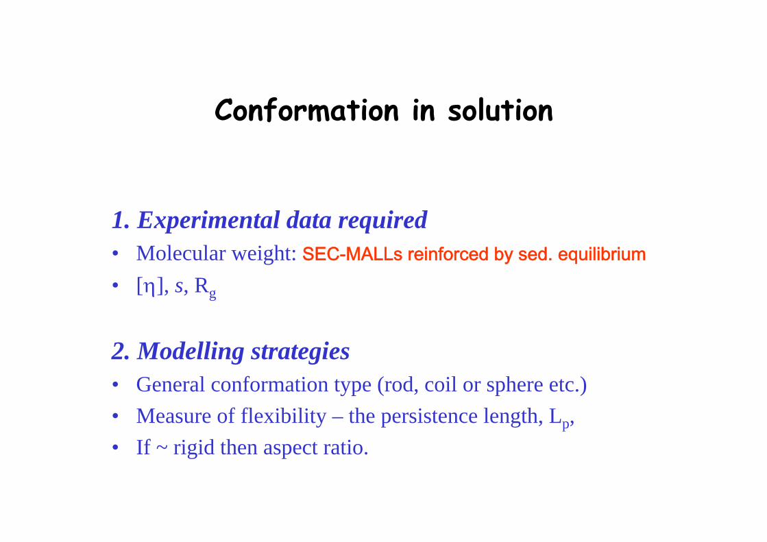
Conformation in solution
1. Experimental data required• Molecular weight: SEC-MALLs reinforced by sed. equilibrium• [η], s, Rg
2. Modelling strategies • General conformation type (rod, coil or sphere etc.)• Measure of flexibility – the persistence length, Lp, • If ~ rigid then aspect ratio.

Sedimentation Velocity
Air Solvent
Solution
conc, c
distance, r
Top view, sector ofcentrifuge cell
Rate of movement ofboundary sed. coeff
Centrifugal force
so20,w
Sedimentation coefficient, S
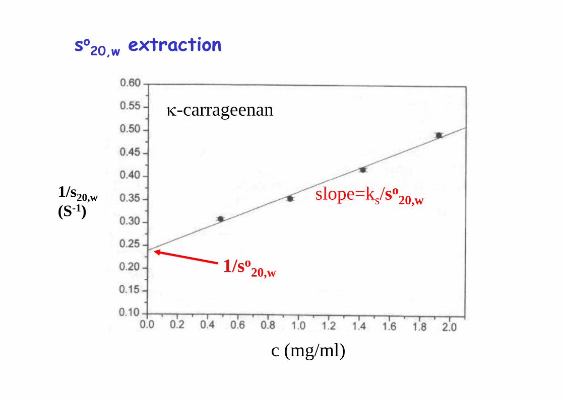
so20,w extraction
κ-carrageenan
1/s20,w(S-1)
c (mg/ml)
1/so20,w
slope=ks/so20,w

Molecular Weight: Zimm plot
1/Mw
sin2(θ/2) + kc (k=100)
106.(Kc/Rθ)
Rg from slope

c (mg/ml)
Kraemer
Huggins
[η]ηred or ηinh(ml/g)
irradiated (10kGy) guar
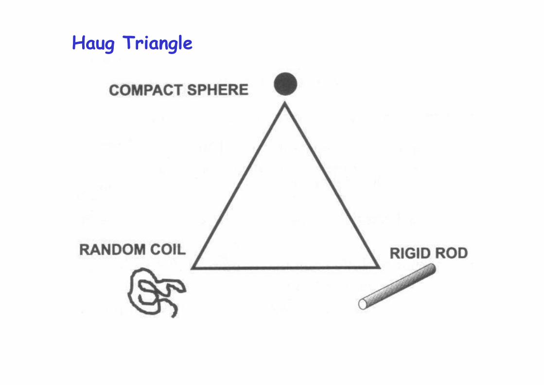
Haug Triangle
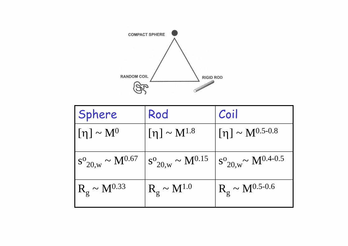
Rg ~ M0.5-0.6Rg ~ M1.0Rg ~ M0.33
so20,w~ M0.4-0.5so
20,w ~ M0.15so20,w ~ M0.67
[η] ~ M0.5-0.8[η] ~ M1.8[η] ~ M0
CoilRodSphere

Mark-Houwink-Kuhn-Sakurada Power law plot
Galactomannansa=0.74+0.01
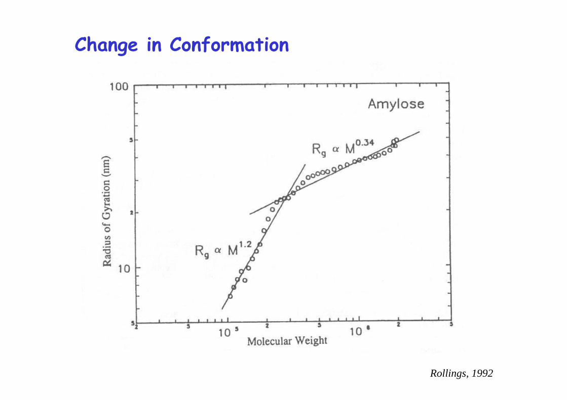
Change in Conformation
Rollings, 1992
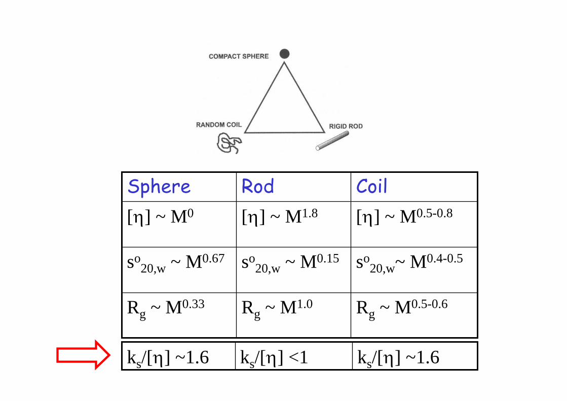
Rg ~ M0.5-0.6Rg ~ M1.0Rg ~ M0.33
so20,w~ M0.4-0.5so
20,w ~ M0.15so20,w ~ M0.67
[η] ~ M0.5-0.8[η] ~ M1.8[η] ~ M0
CoilRodSphere
ks/[η] ~1.6ks/[η] <1ks/[η] ~1.6
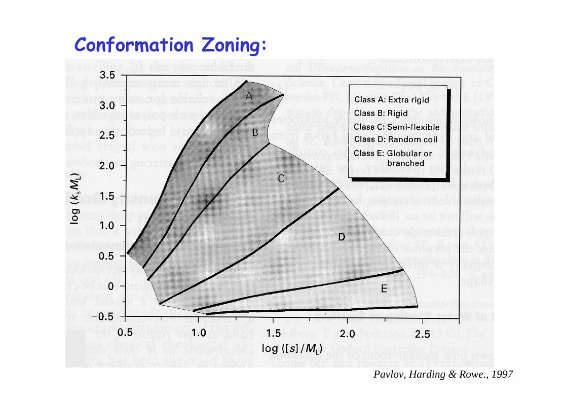
Conformation Zoning:
Pavlov, Harding & Rowe., 1997
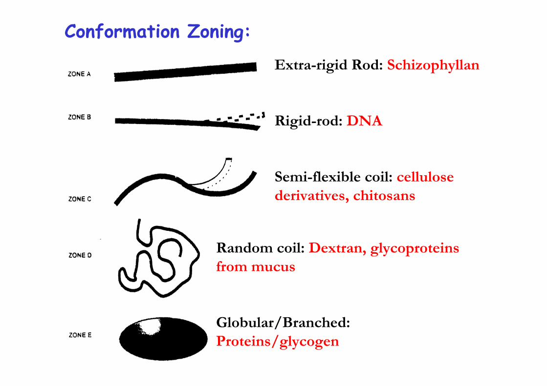
Conformation Zoning:
Extra-rigid Rod: Schizophyllan
Rigid-rod: DNA
Semi-flexible coil: cellulose derivatives, chitosans
Random coil: Dextran, glycoproteinsfrom mucus
Globular/Branched: Proteins/glycogen
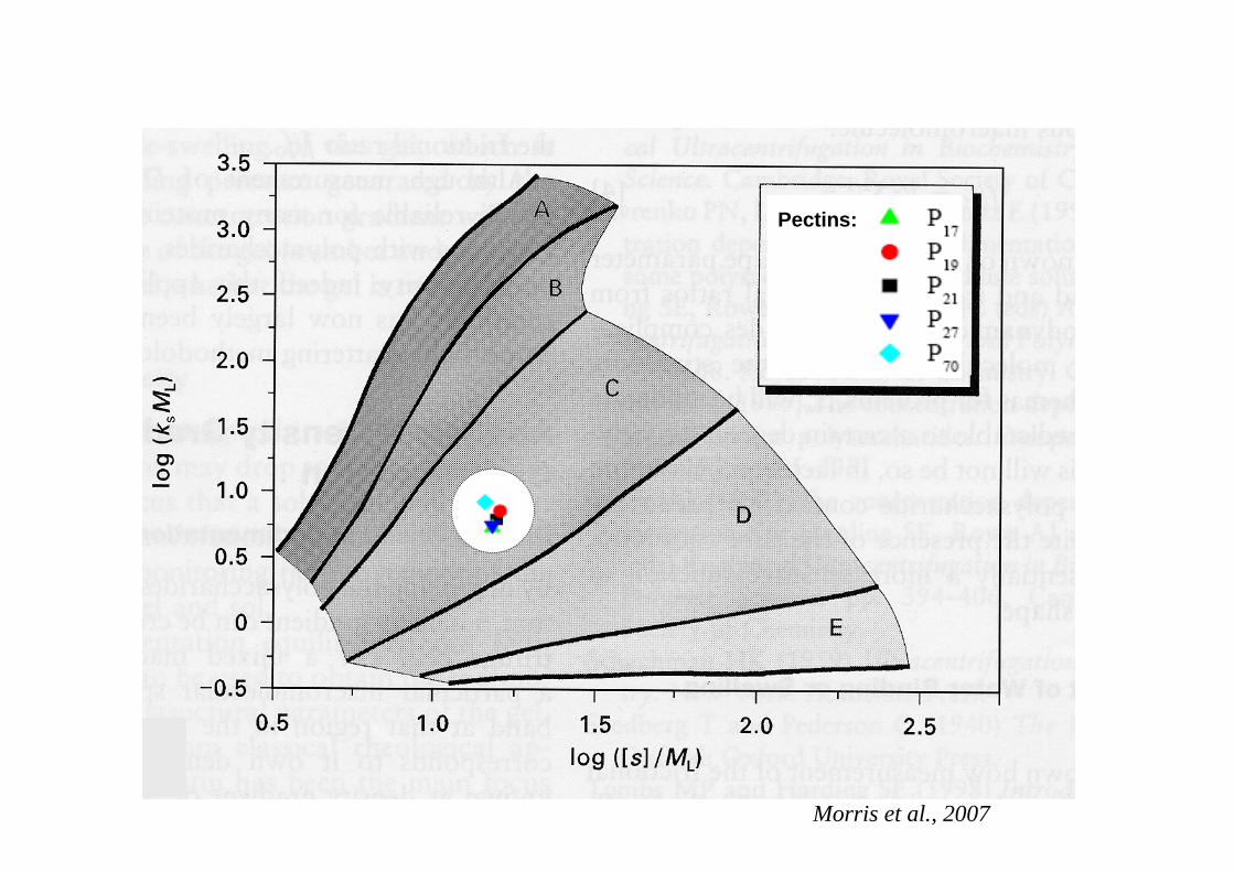
Morris et al., 2007
Pectins:
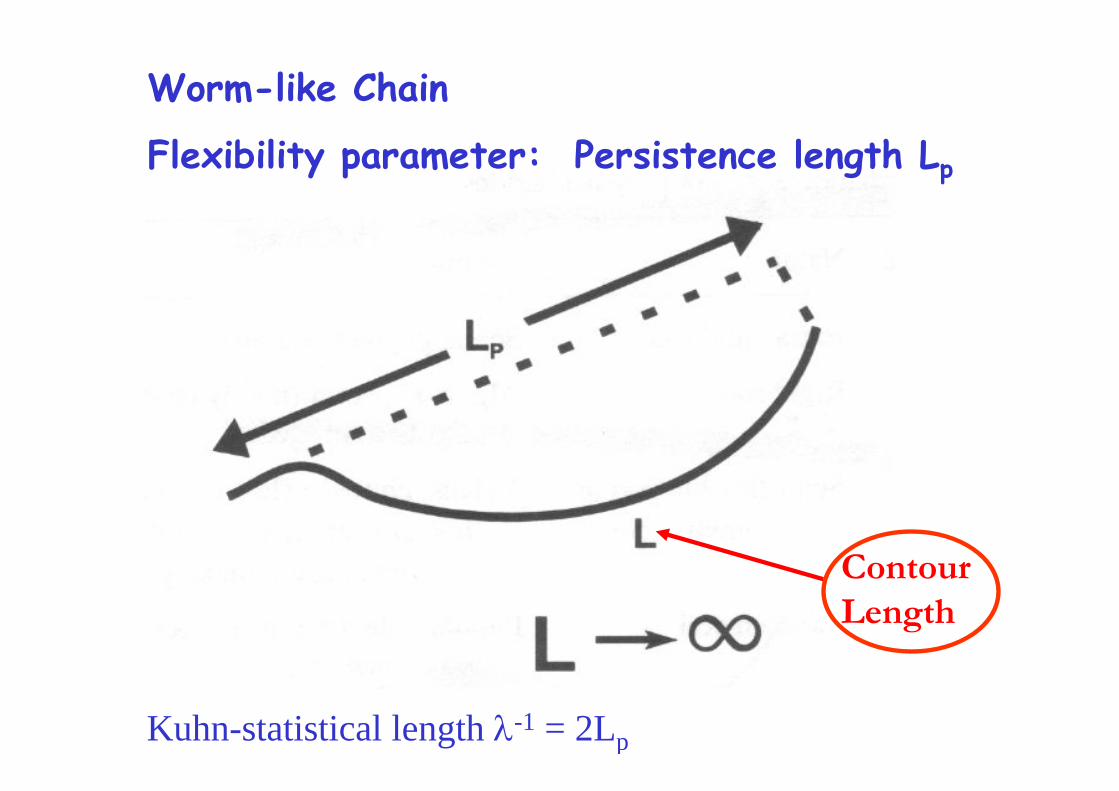
Contour Length
Worm-like Chain
Flexibility parameter: Persistence length Lp
Kuhn-statistical length λ-1 = 2Lp
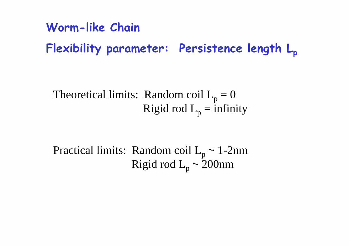
Worm-like Chain
Flexibility parameter: Persistence length Lp
Theoretical limits: Random coil Lp = 0Rigid rod Lp = infinity
Practical limits: Random coil Lp ~ 1-2nmRigid rod Lp ~ 200nm
[ ]2/1
2/13/1
03/1
0
3/12 2w
L
pL
w MML
BMAM
−
−−⎟⎟⎠
⎞⎜⎜⎝
⎛Φ+Φ=⎟⎟
⎠
⎞⎜⎜⎝
⎛η
( )⎥⎥
⎦
⎤
⎢⎢
⎣
⎡+⎟
⎟⎠
⎞⎜⎜⎝
⎛++⎟
⎟⎠
⎞⎜⎜⎝
⎛×
−=
−
....22
843.13
12/1
32
2/1
0
00
pL
w
pL
w
A
L
LMM
AALM
MNvM
sπη
ρ
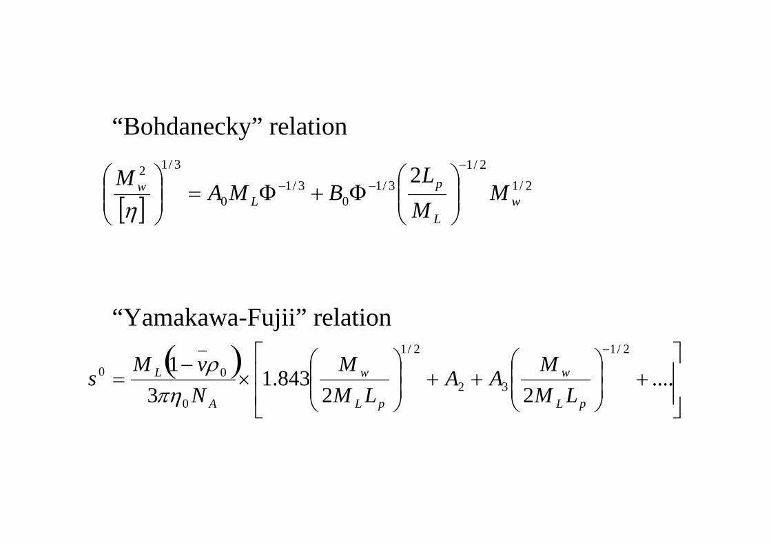
“Bohdanecky” relation
“Yamakawa-Fujii” relation
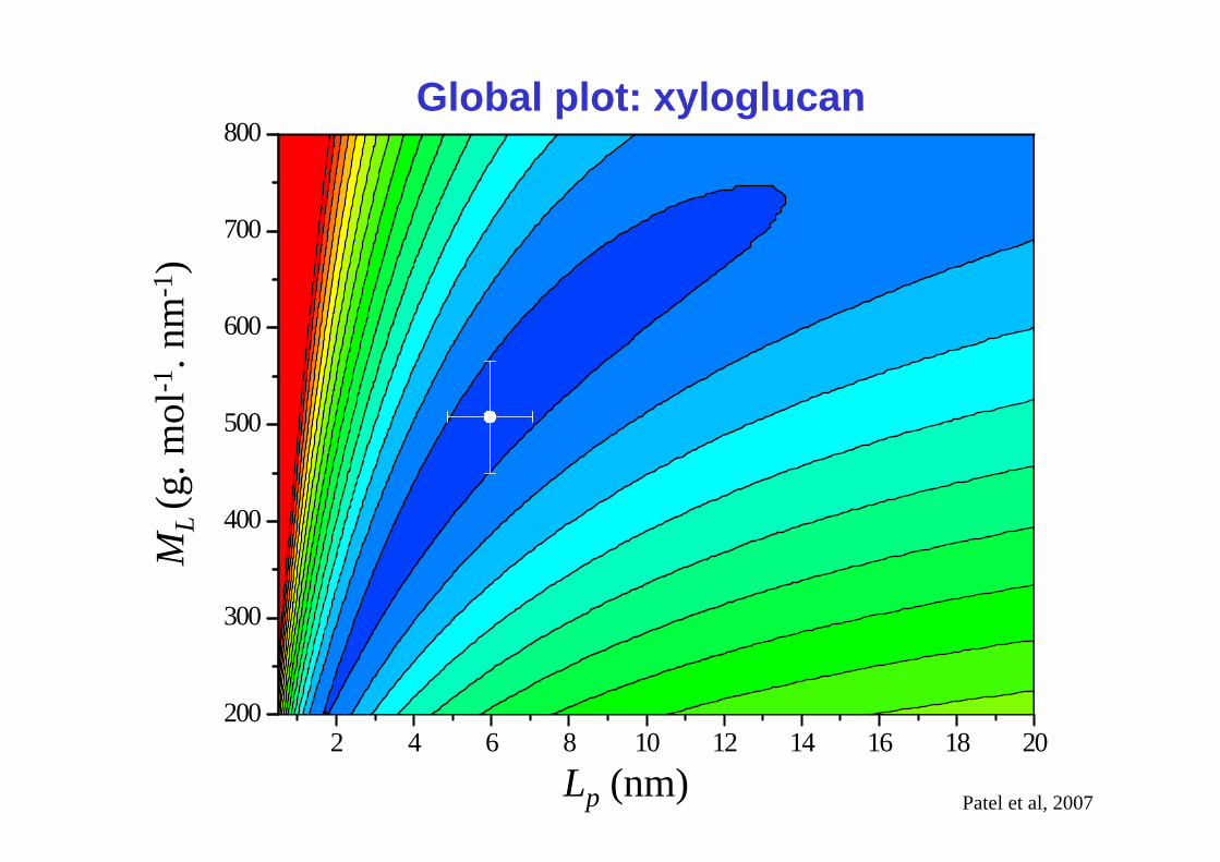
Global plot: xyloglucan
2 4 6 8 10 12 14 16 18 20200
300
400
500
600
700
800M
L(g
. mol
-1. n
m-1
)
Lp (nm) Patel et al, 2007
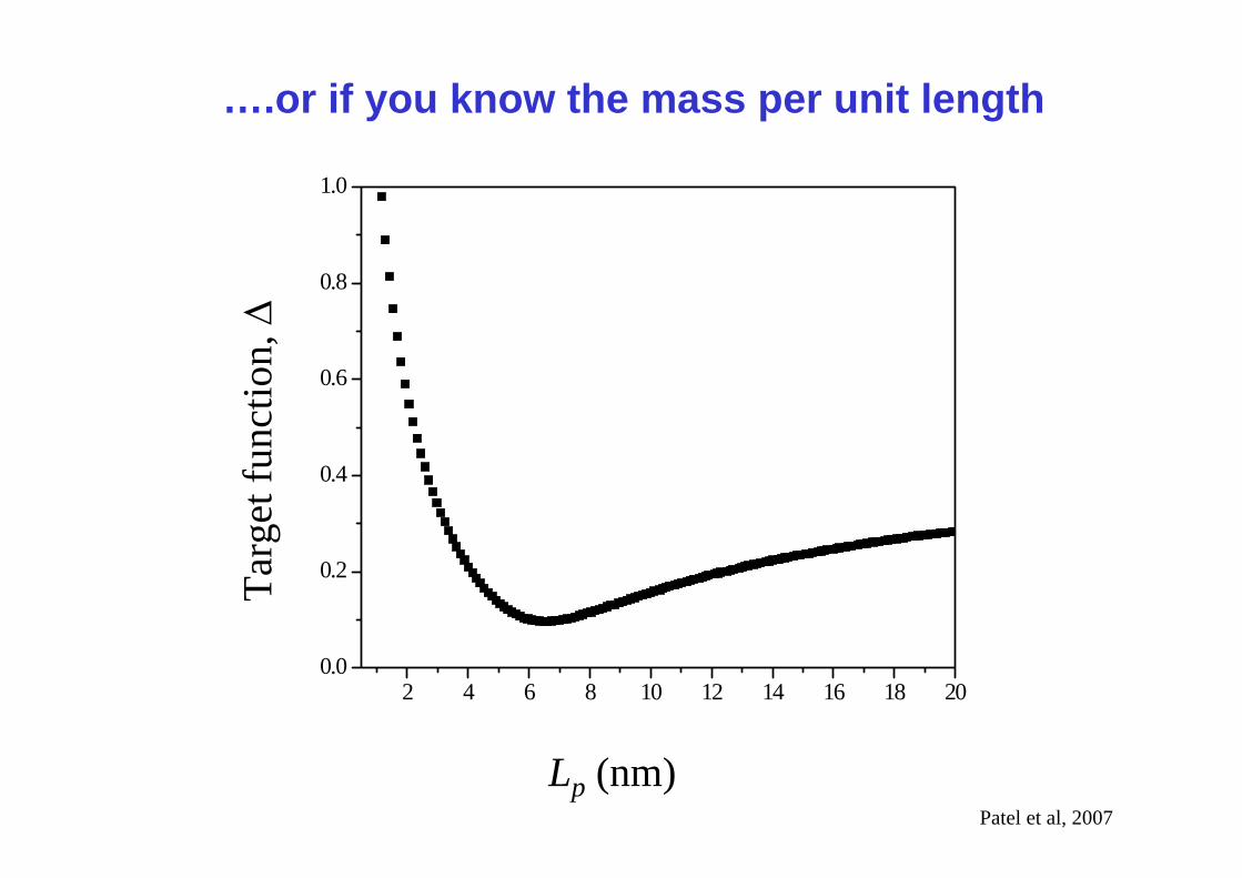
….or if you know the mass per unit length
Lp (nm)
2 4 6 8 10 12 14 16 18 200.0
0.2
0.4
0.6
0.8
1.0
Targ
et fu
nctio
n, Δ
Patel et al, 2007
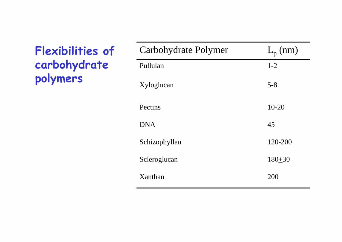
200Xanthan
180+30Scleroglucan
120-200Schizophyllan
45DNA
10-20Pectins
5-8Xyloglucan
1-2Pullulan
Lp (nm)Carbohydrate PolymerFlexibilities of carbohydrate polymers
4. Interactions
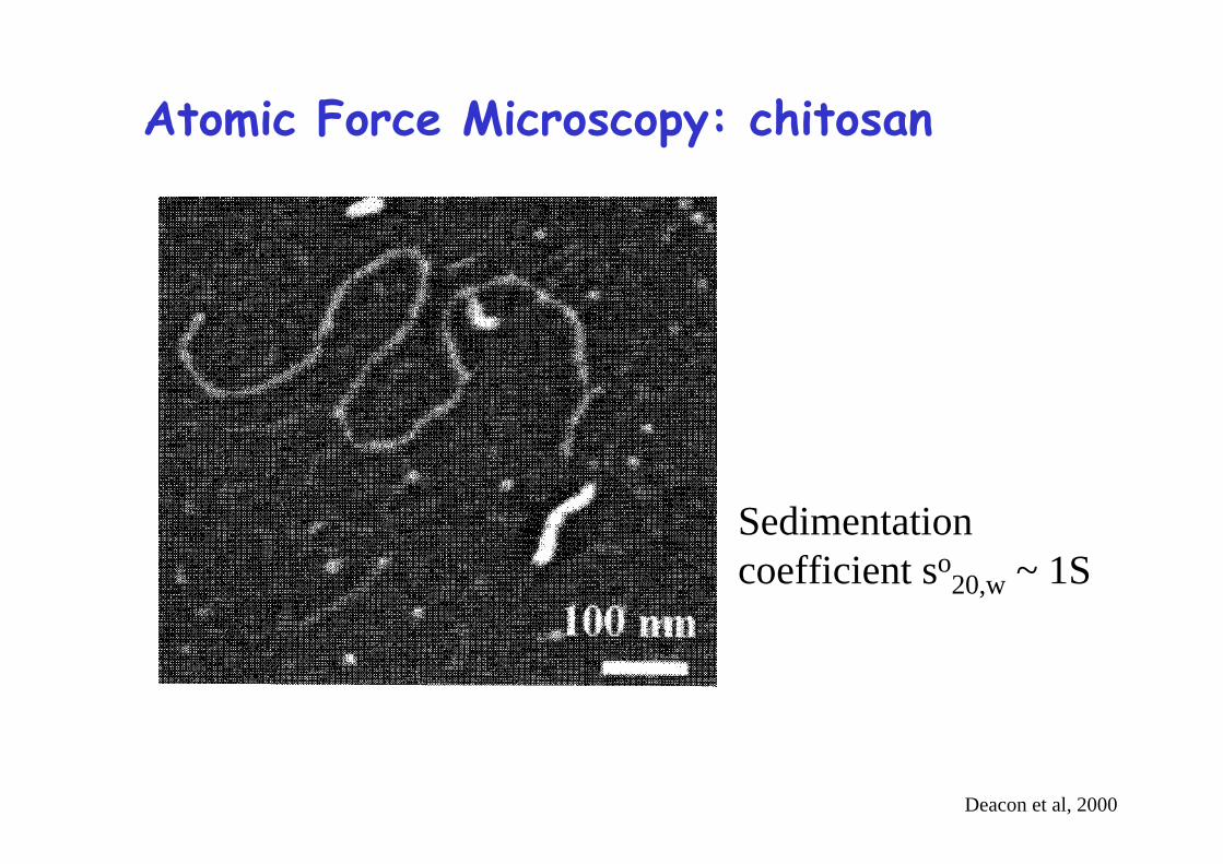
Atomic Force Microscopy: chitosan
Sedimentation coefficient so
20,w ~ 1S
Deacon et al, 2000
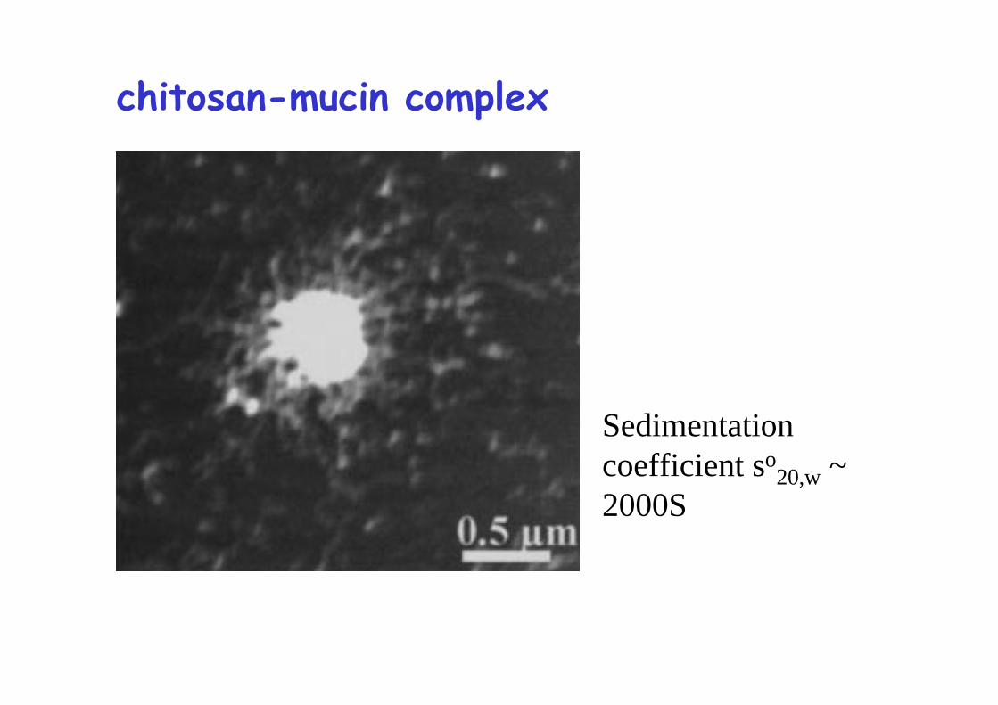
chitosan-mucin complex
Sedimentation coefficient so
20,w ~ 2000S
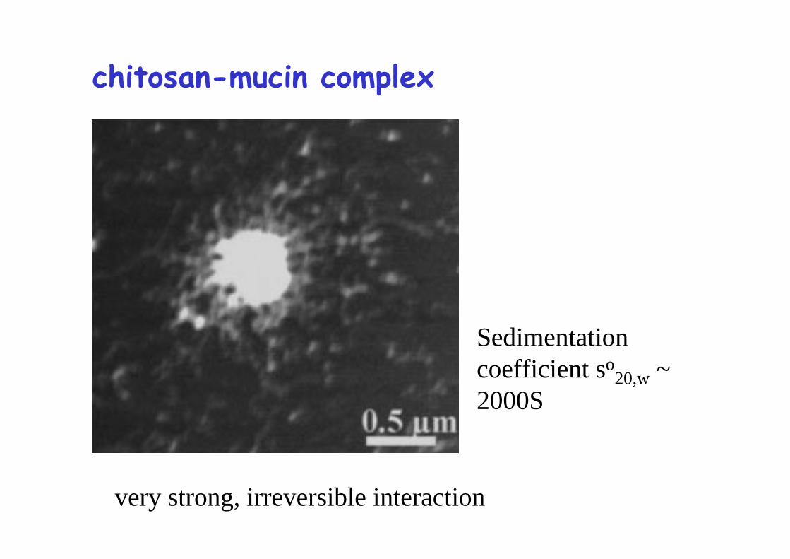
chitosan-mucin complex
Sedimentation coefficient so
20,w ~ 2000S
very strong, irreversible interaction
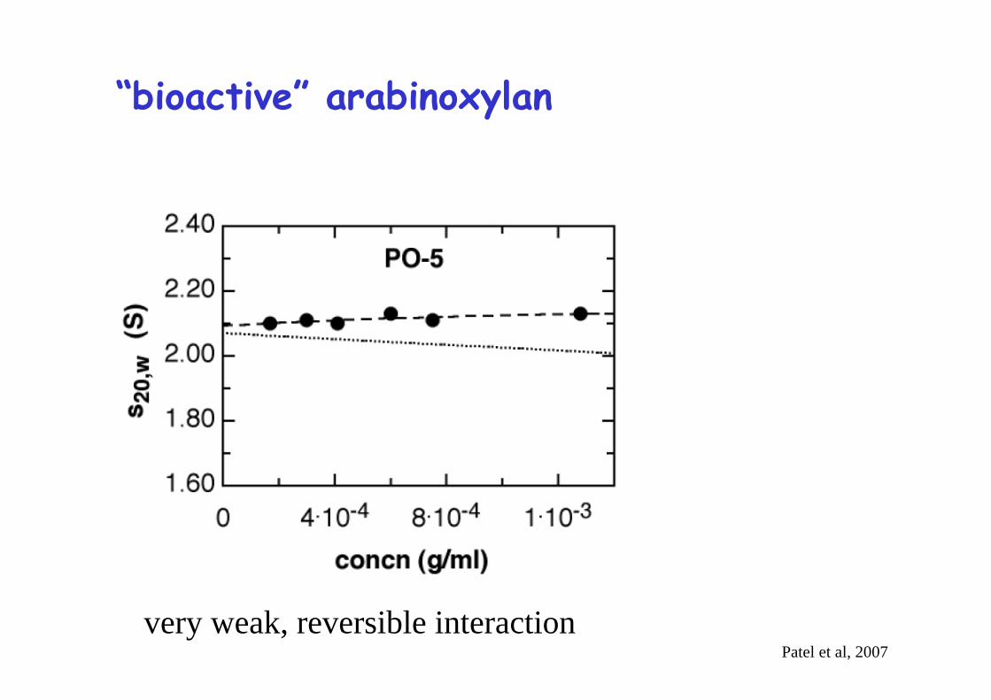
“bioactive” arabinoxylan
very weak, reversible interactionPatel et al, 2007
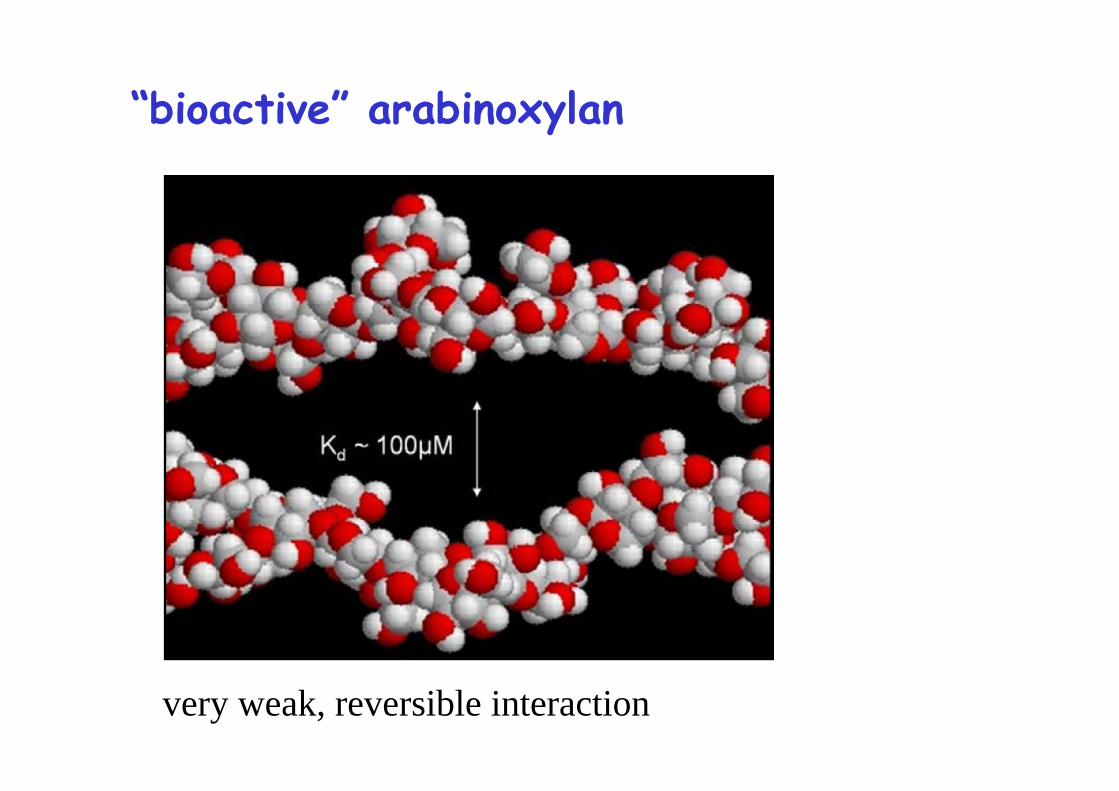
“bioactive” arabinoxylan
very weak, reversible interaction
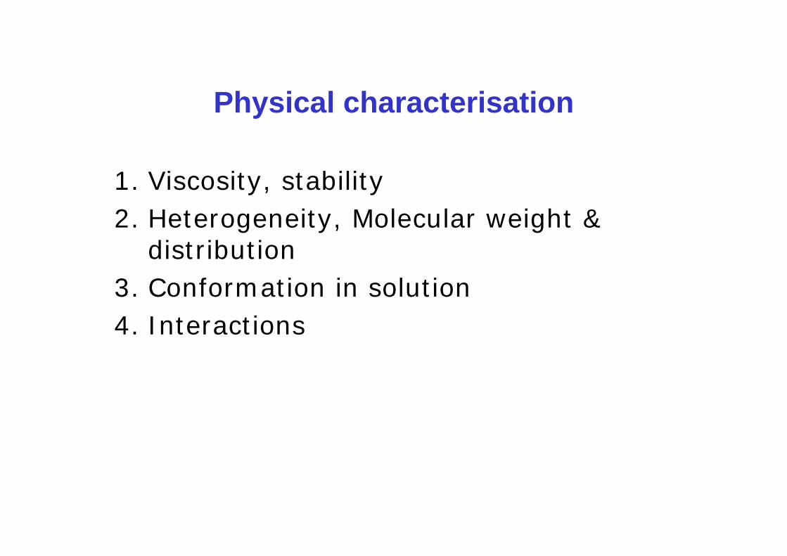
Physical characterisation
1. Viscosity, stability2. Heterogeneity, Molecular weight &
distribution3. Conformation in solution4. Interactions
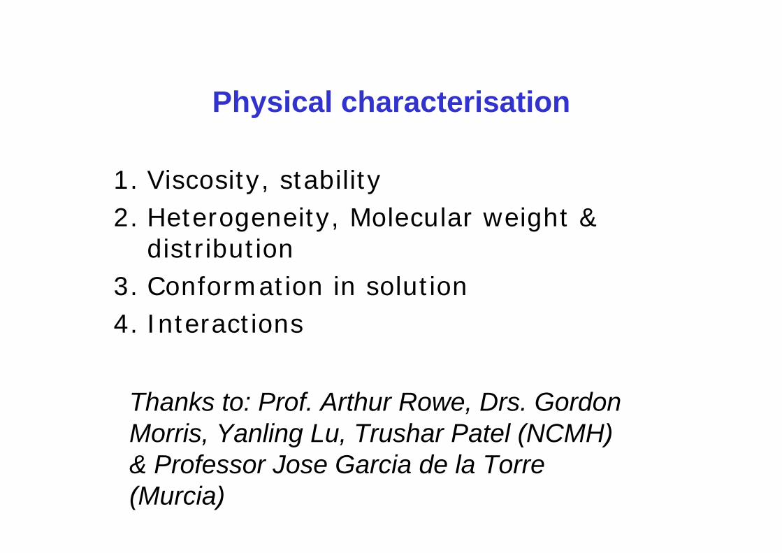
Physical characterisation
1. Viscosity, stability2. Heterogeneity, Molecular weight &
distribution3. Conformation in solution4. Interactions
Thanks to: Prof. Arthur Rowe, Drs. Gordon Morris, Yanling Lu, Trushar Patel (NCMH) & Professor Jose Garcia de la Torre (Murcia)
for a copy of this presentation …
http://www.nottingham.ac.uk/ncmh