The p-adic L-functions of an evil Eisenstein...
98
The p-adic L-functions of an evil Eisenstein Series Joint work with Samit Dasgupta Luminy, June 2011 Jo¨ el Bella¨ ıche June 27, 2011
Transcript of The p-adic L-functions of an evil Eisenstein...
The p-adic L-functions of an evil Eisenstein SeriesJoint work with Samit Dasgupta
Luminy, June 2011
Joel Bellaıche
June 27, 2011
Refinement of a modular form (why?)
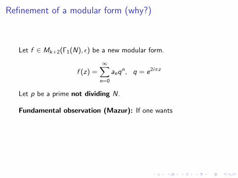
Let f ∈ Mk+2(Γ1(N), ε) be a new modular form.
f (z) =∞∑
n=0
anqn, q = e2iπz
Let p be a prime not dividing N.
Fundamental observation (Mazur): If one wants (a) to attach ap-adic L-function to f , or (b) to put f in a p-adic family of modularforms, the form f is not the right object. We need to refine it.
Refinement of a modular form (why?)
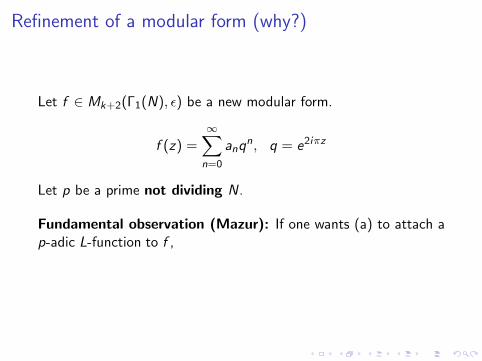
Let f ∈ Mk+2(Γ1(N), ε) be a new modular form.
f (z) =∞∑
n=0
anqn, q = e2iπz
Let p be a prime not dividing N.
Fundamental observation (Mazur): If one wants (a) to attach ap-adic L-function to f , or (b) to put f in a p-adic family of modularforms, the form f is not the right object. We need to refine it.
Refinement of a modular form (why?)
Let f ∈ Mk+2(Γ1(N), ε) be a new modular form.
f (z) =∞∑
n=0
anqn, q = e2iπz
Let p be a prime not dividing N.
Fundamental observation (Mazur): If one wants
(a) to attach ap-adic L-function to f , or (b) to put f in a p-adic family of modularforms, the form f is not the right object. We need to refine it.
Refinement of a modular form (why?)
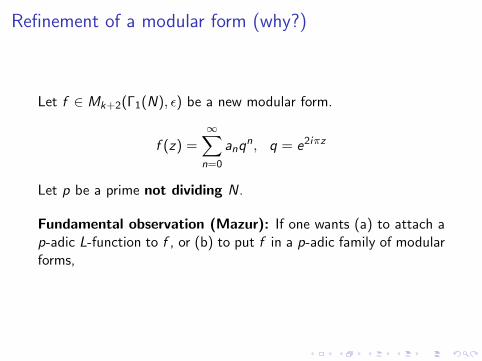
Let f ∈ Mk+2(Γ1(N), ε) be a new modular form.
f (z) =∞∑
n=0
anqn, q = e2iπz
Let p be a prime not dividing N.
Fundamental observation (Mazur): If one wants (a) to attach ap-adic L-function to f ,
or (b) to put f in a p-adic family of modularforms, the form f is not the right object. We need to refine it.
Refinement of a modular form (why?)
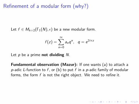
Let f ∈ Mk+2(Γ1(N), ε) be a new modular form.
f (z) =∞∑
n=0
anqn, q = e2iπz
Let p be a prime not dividing N.
Fundamental observation (Mazur): If one wants (a) to attach ap-adic L-function to f , or (b) to put f in a p-adic family of modularforms,
the form f is not the right object. We need to refine it.
Refinement of a modular form (why?)
Let f ∈ Mk+2(Γ1(N), ε) be a new modular form.
f (z) =∞∑
n=0
anqn, q = e2iπz
Let p be a prime not dividing N.
Fundamental observation (Mazur): If one wants (a) to attach ap-adic L-function to f , or (b) to put f in a p-adic family of modularforms, the form f is not the right object. We need to refine it.
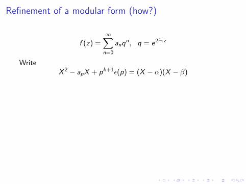
Refinement of a modular form (how?)
f (z) =∞∑
n=0
anqn, q = e2iπz
WriteX 2 − apX + pk+1ε(p) = (X − α)(X − β)
One has 0 ≤ vp(α), vp(β) ≤ k + 1 and vp(α) + vp(β) = k + 1. Ifα 6= β, there are exactly two normalized forms of levelΓ := Γ1(N) ∩ Γ0(p), nebentypus ε, that are eigenforms for Up andfor all Hecke operators Tl , l 6 |Np with same eigenvalues as f :
fα(z) = f (z)− βf (pz), Upfα = αfα
fβ(z) = f (z)− αf (pz), Upfβ = βfβ
To refine f is to choose one of those forms. The forms fα and fβare called refinements of f .
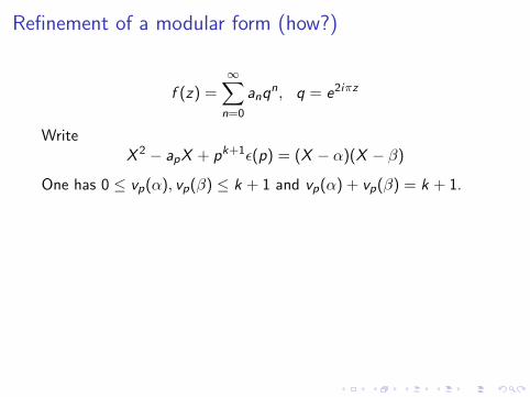
Refinement of a modular form (how?)
f (z) =∞∑
n=0
anqn, q = e2iπz
WriteX 2 − apX + pk+1ε(p) = (X − α)(X − β)
One has 0 ≤ vp(α), vp(β) ≤ k + 1 and vp(α) + vp(β) = k + 1.
Ifα 6= β, there are exactly two normalized forms of levelΓ := Γ1(N) ∩ Γ0(p), nebentypus ε, that are eigenforms for Up andfor all Hecke operators Tl , l 6 |Np with same eigenvalues as f :
fα(z) = f (z)− βf (pz), Upfα = αfα
fβ(z) = f (z)− αf (pz), Upfβ = βfβ
To refine f is to choose one of those forms. The forms fα and fβare called refinements of f .
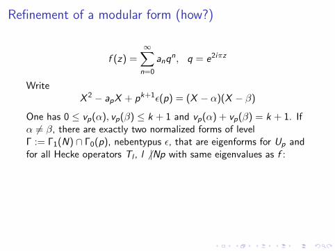
Refinement of a modular form (how?)
f (z) =∞∑
n=0
anqn, q = e2iπz
WriteX 2 − apX + pk+1ε(p) = (X − α)(X − β)
One has 0 ≤ vp(α), vp(β) ≤ k + 1 and vp(α) + vp(β) = k + 1. Ifα 6= β, there are exactly two normalized forms of levelΓ := Γ1(N) ∩ Γ0(p), nebentypus ε, that are eigenforms for Up andfor all Hecke operators Tl , l 6 |Np with same eigenvalues as f :
fα(z) = f (z)− βf (pz), Upfα = αfα
fβ(z) = f (z)− αf (pz), Upfβ = βfβ
To refine f is to choose one of those forms. The forms fα and fβare called refinements of f .
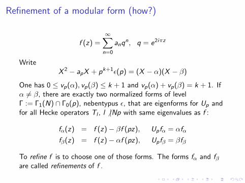
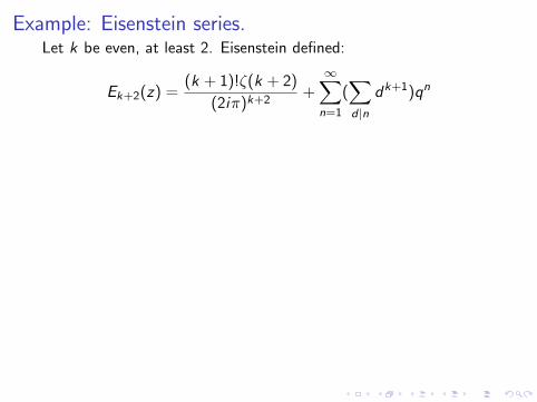
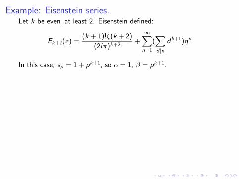
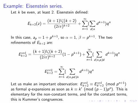
Example: Eisenstein series.Let k be even, at least 2. Eisenstein defined:
Ek+2(z) =(k + 1)!ζ(k + 2)
(2iπ)k+2+∞∑
n=1
(∑d |n
dk+1)qn
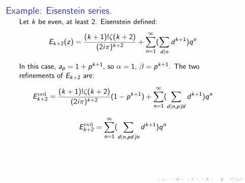
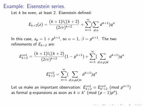
In this case, ap = 1 + pk+1, so α = 1, β = pk+1. The tworefinements of Ek+2 are:
E ordk+2 =
(k + 1)!ζ(k + 2)
(2iπ)k+2(1− pk+1) +
∞∑n=1
(∑
d |n,p 6 |d
dk+1)qn
E evilk+2 =
∞∑n=1
(∑
d |n,pd 6 |n
dk+1)qn
Let us make an important observation: E ordk+2 ≡ E ord
k ′+2 (mod pn+1)as formal q-expansions as soon as k ≡ k ′ (mod (p − 1)pn). This iselementary for the non-constant terms, and for the constant terms,this is Kummer’s congruences.
Example: Eisenstein series.Let k be even, at least 2. Eisenstein defined:
Ek+2(z) =(k + 1)!ζ(k + 2)
(2iπ)k+2+∞∑
n=1
(∑d |n
dk+1)qn
In this case, ap = 1 + pk+1, so α = 1, β = pk+1.
The tworefinements of Ek+2 are:
E ordk+2 =
(k + 1)!ζ(k + 2)
(2iπ)k+2(1− pk+1) +
∞∑n=1
(∑
d |n,p 6 |d
dk+1)qn
E evilk+2 =
∞∑n=1
(∑
d |n,pd 6 |n
dk+1)qn
Let us make an important observation: E ordk+2 ≡ E ord
k ′+2 (mod pn+1)as formal q-expansions as soon as k ≡ k ′ (mod (p − 1)pn). This iselementary for the non-constant terms, and for the constant terms,this is Kummer’s congruences.
Example: Eisenstein series.Let k be even, at least 2. Eisenstein defined:
Ek+2(z) =(k + 1)!ζ(k + 2)
(2iπ)k+2+∞∑
n=1
(∑d |n
dk+1)qn
In this case, ap = 1 + pk+1, so α = 1, β = pk+1. The tworefinements of Ek+2 are:
E ordk+2 =
(k + 1)!ζ(k + 2)
(2iπ)k+2(1− pk+1) +
∞∑n=1
(∑
d |n,p 6 |d
dk+1)qn
E evilk+2 =
∞∑n=1
(∑
d |n,pd 6 |n
dk+1)qn
Let us make an important observation: E ordk+2 ≡ E ord
k ′+2 (mod pn+1)as formal q-expansions as soon as k ≡ k ′ (mod (p − 1)pn). This iselementary for the non-constant terms, and for the constant terms,this is Kummer’s congruences.
Example: Eisenstein series.Let k be even, at least 2. Eisenstein defined:
Ek+2(z) =(k + 1)!ζ(k + 2)
(2iπ)k+2+∞∑
n=1
(∑d |n
dk+1)qn
In this case, ap = 1 + pk+1, so α = 1, β = pk+1. The tworefinements of Ek+2 are:
E ordk+2 =
(k + 1)!ζ(k + 2)
(2iπ)k+2(1− pk+1) +
∞∑n=1
(∑
d |n,p 6 |d
dk+1)qn
E evilk+2 =
∞∑n=1
(∑
d |n,pd 6 |n
dk+1)qn
Let us make an important observation: E ordk+2 ≡ E ord
k ′+2 (mod pn+1)as formal q-expansions as soon as k ≡ k ′ (mod (p − 1)pn).
This iselementary for the non-constant terms, and for the constant terms,this is Kummer’s congruences.
Example: Eisenstein series.Let k be even, at least 2. Eisenstein defined:
Ek+2(z) =(k + 1)!ζ(k + 2)
(2iπ)k+2+∞∑
n=1
(∑d |n
dk+1)qn
In this case, ap = 1 + pk+1, so α = 1, β = pk+1. The tworefinements of Ek+2 are:
E ordk+2 =
(k + 1)!ζ(k + 2)
(2iπ)k+2(1− pk+1) +
∞∑n=1
(∑
d |n,p 6 |d
dk+1)qn
E evilk+2 =
∞∑n=1
(∑
d |n,pd 6 |n
dk+1)qn
Let us make an important observation: E ordk+2 ≡ E ord
k ′+2 (mod pn+1)as formal q-expansions as soon as k ≡ k ′ (mod (p − 1)pn). This iselementary for the non-constant terms, and for the constant terms,this is Kummer’s congruences.
Example: Eisenstein series.
Hence the E ordk+2’s belong to a p-adic family of ordinary Eisensteins
series.
On the contrary, E evilk+2 does not belong to a p-adic family of
Eisenstein series. It belongs to a p-adic family of modular forms,though, as shown by Coleman, but it siblings are cuspidal, notEisenstein. In many p-adic respects, E evil
k+2 behaves like a cuspidal
form. Like The Ugly Duckling, E evilk+2, born by mistake among
Eisenstein ducks, eventually joined its true family of cuspidal swans.
Example: Eisenstein series.
Hence the E ordk+2’s belong to a p-adic family of ordinary Eisensteins
series.
On the contrary, E evilk+2 does not belong to a p-adic family of
Eisenstein series.
It belongs to a p-adic family of modular forms,though, as shown by Coleman, but it siblings are cuspidal, notEisenstein. In many p-adic respects, E evil
k+2 behaves like a cuspidal
form. Like The Ugly Duckling, E evilk+2, born by mistake among
Eisenstein ducks, eventually joined its true family of cuspidal swans.
Example: Eisenstein series.
Hence the E ordk+2’s belong to a p-adic family of ordinary Eisensteins
series.
On the contrary, E evilk+2 does not belong to a p-adic family of
Eisenstein series. It belongs to a p-adic family of modular forms,though, as shown by Coleman, but it siblings are cuspidal, notEisenstein.
In many p-adic respects, E evilk+2 behaves like a cuspidal
form. Like The Ugly Duckling, E evilk+2, born by mistake among
Eisenstein ducks, eventually joined its true family of cuspidal swans.
Example: Eisenstein series.
Hence the E ordk+2’s belong to a p-adic family of ordinary Eisensteins
series.
On the contrary, E evilk+2 does not belong to a p-adic family of
Eisenstein series. It belongs to a p-adic family of modular forms,though, as shown by Coleman, but it siblings are cuspidal, notEisenstein. In many p-adic respects, E evil
k+2 behaves like a cuspidal
form. Like The Ugly Duckling, E evilk+2, born by mistake among
Eisenstein ducks, eventually joined its true family of cuspidal swans.
p-adic L-functions: classical results
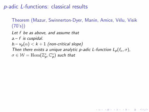
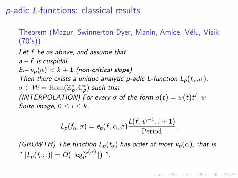
Theorem (Mazur, Swinnerton-Dyer, Manin, Amice, Velu, Visik(70’s))
Let f be as above, and assume thata.– f is cuspidal.b.– vp(α) < k + 1 (non-critical slope)Then there exists a unique analytic p-adic L-function Lp(fα, σ),σ ∈ W = Hom(Z∗p,C∗p) such that
(INTERPOLATION) For every σ of the form σ(t) = ψ(t)t i , ψfinite image, 0 ≤ i ≤ k,
Lp(fα, σ) = ep(f , α, σ)L(f , ψ−1, i + 1)
Period.
(GROWTH) The function Lp(fα) has order at most vp(α), that is
” |Lp(fα, .)| = O(| logvp(α)p |) ”.
p-adic L-functions: classical results
Theorem (Mazur, Swinnerton-Dyer, Manin, Amice, Velu, Visik(70’s))
Let f be as above, and assume thata.– f is cuspidal.
b.– vp(α) < k + 1 (non-critical slope)Then there exists a unique analytic p-adic L-function Lp(fα, σ),σ ∈ W = Hom(Z∗p,C∗p) such that
(INTERPOLATION) For every σ of the form σ(t) = ψ(t)t i , ψfinite image, 0 ≤ i ≤ k,
Lp(fα, σ) = ep(f , α, σ)L(f , ψ−1, i + 1)
Period.
(GROWTH) The function Lp(fα) has order at most vp(α), that is
” |Lp(fα, .)| = O(| logvp(α)p |) ”.
p-adic L-functions: classical results
Theorem (Mazur, Swinnerton-Dyer, Manin, Amice, Velu, Visik(70’s))
Let f be as above, and assume thata.– f is cuspidal.b.– vp(α) < k + 1 (non-critical slope)
Then there exists a unique analytic p-adic L-function Lp(fα, σ),σ ∈ W = Hom(Z∗p,C∗p) such that
(INTERPOLATION) For every σ of the form σ(t) = ψ(t)t i , ψfinite image, 0 ≤ i ≤ k,
Lp(fα, σ) = ep(f , α, σ)L(f , ψ−1, i + 1)
Period.
(GROWTH) The function Lp(fα) has order at most vp(α), that is
” |Lp(fα, .)| = O(| logvp(α)p |) ”.
p-adic L-functions: classical results
Theorem (Mazur, Swinnerton-Dyer, Manin, Amice, Velu, Visik(70’s))
Let f be as above, and assume thata.– f is cuspidal.b.– vp(α) < k + 1 (non-critical slope)Then there exists a unique analytic p-adic L-function Lp(fα, σ),σ ∈ W = Hom(Z∗p,C∗p) such that
(INTERPOLATION) For every σ of the form σ(t) = ψ(t)t i , ψfinite image, 0 ≤ i ≤ k,
Lp(fα, σ) = ep(f , α, σ)L(f , ψ−1, i + 1)
Period.
(GROWTH) The function Lp(fα) has order at most vp(α), that is
” |Lp(fα, .)| = O(| logvp(α)p |) ”.
p-adic L-functions: classical results
Theorem (Mazur, Swinnerton-Dyer, Manin, Amice, Velu, Visik(70’s))
Let f be as above, and assume thata.– f is cuspidal.b.– vp(α) < k + 1 (non-critical slope)Then there exists a unique analytic p-adic L-function Lp(fα, σ),σ ∈ W = Hom(Z∗p,C∗p) such that
(INTERPOLATION) For every σ of the form σ(t) = ψ(t)t i , ψfinite image, 0 ≤ i ≤ k,
Lp(fα, σ) = ep(f , α, σ)L(f , ψ−1, i + 1)
Period.
(GROWTH) The function Lp(fα) has order at most vp(α), that is
” |Lp(fα, .)| = O(| logvp(α)p |) ”.
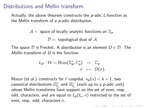
Distributions and Mellin transform
Actually, the above theorem constructs the p-adic L-function asthe Mellin transform of a p-adic distribution.
A = space of locally analytic functions on Zp
D = topological dual of A
The space D is Frechet. A distribution is an element D ∈ D. TheMellin transform of D is the function
LD :W = Hom(Z∗p,C∗p) → Cp
σ 7→ D(σ).
Mazur (et al.) constructs for f cuspidal, vp(α) < k + 1, twocanonical distributions D+
fαand D−fα (each up to a p-adic unit)
whose Mellin transforms have support on the set of even, resp.odd, characters, and are equal to Lp(fα, σ) restricted to the set ofeven, resp. odd, characters σ.
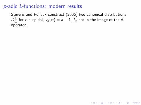
p-adic L-functions: modern results
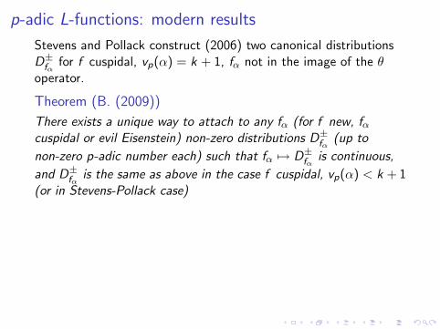
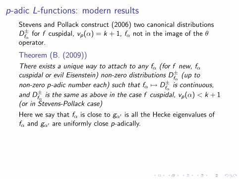
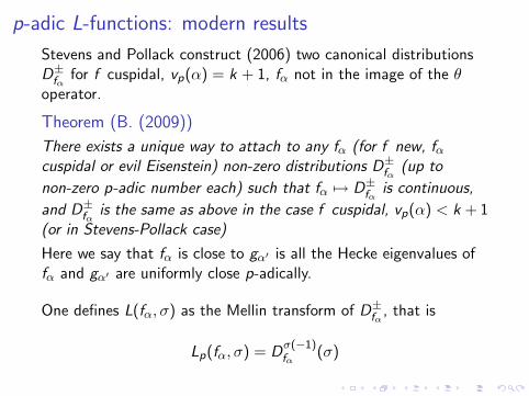
Stevens and Pollack construct (2006) two canonical distributionsD±fα for f cuspidal, vp(α) = k + 1, fα not in the image of the θoperator.
Theorem (B. (2009))
There exists a unique way to attach to any fα (for f new, fαcuspidal or evil Eisenstein) non-zero distributions D±fα (up to
non-zero p-adic number each) such that fα 7→ D±fα is continuous,
and D±fα is the same as above in the case f cuspidal, vp(α) < k + 1(or in Stevens-Pollack case)
Here we say that fα is close to gα′ is all the Hecke eigenvalues offα and gα′ are uniformly close p-adically.
One defines L(fα, σ) as the Mellin transform of D±fα , that is
Lp(fα, σ) = Dσ(−1)fα
(σ)
p-adic L-functions: modern results
Stevens and Pollack construct (2006) two canonical distributionsD±fα for f cuspidal, vp(α) = k + 1, fα not in the image of the θoperator.
Theorem (B. (2009))
There exists a unique way to attach to any fα (for f new, fαcuspidal or evil Eisenstein) non-zero distributions D±fα (up to
non-zero p-adic number each) such that fα 7→ D±fα is continuous,
and D±fα is the same as above in the case f cuspidal, vp(α) < k + 1(or in Stevens-Pollack case)
Here we say that fα is close to gα′ is all the Hecke eigenvalues offα and gα′ are uniformly close p-adically.
One defines L(fα, σ) as the Mellin transform of D±fα , that is
Lp(fα, σ) = Dσ(−1)fα
(σ)
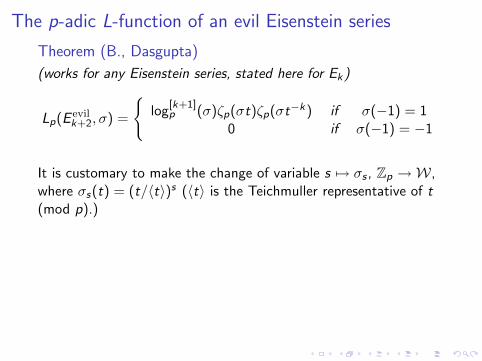
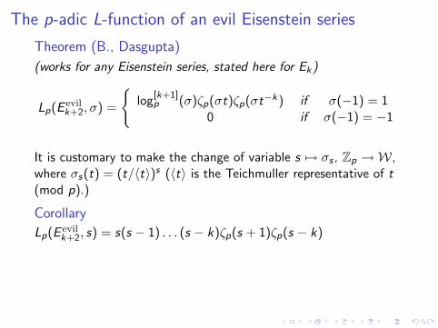
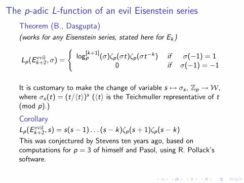
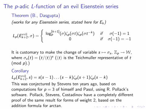
The p-adic L-function of an evil Eisenstein series
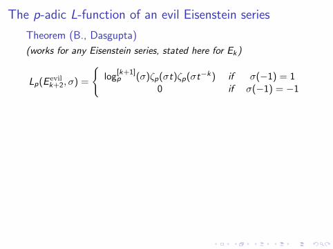
Theorem (B., Dasgupta)
(works for any Eisenstein series, stated here for Ek)
Lp(E evilk+2, σ) =
{log
[k+1]p (σ)ζp(σt)ζp(σt−k) if σ(−1) = 1
0 if σ(−1) = −1
It is customary to make the change of variable s 7→ σs , Zp →W,where σs(t) = (t/〈t〉)s (〈t〉 is the Teichmuller representative of t(mod p).)
Corollary
Lp(E evilk+2, s) = s(s − 1) . . . (s − k)ζp(s + 1)ζp(s − k)
This was conjectured by Stevens ten years ago, based oncomputations for p = 3 of himself and Pasol, using R. Pollack’ssoftware. Pollack, Stevens, Costadinov have a completely differentproof of the same result for forms of weight 2, based on theaddition formula for arctan.
The p-adic L-function of an evil Eisenstein series
Theorem (B., Dasgupta)
(works for any Eisenstein series, stated here for Ek)
Lp(E evilk+2, σ) =
{log
[k+1]p (σ)ζp(σt)ζp(σt−k) if σ(−1) = 1
0 if σ(−1) = −1
It is customary to make the change of variable s 7→ σs , Zp →W,where σs(t) = (t/〈t〉)s (〈t〉 is the Teichmuller representative of t(mod p).)
Corollary
Lp(E evilk+2, s) = s(s − 1) . . . (s − k)ζp(s + 1)ζp(s − k)
This was conjectured by Stevens ten years ago, based oncomputations for p = 3 of himself and Pasol, using R. Pollack’ssoftware.
Pollack, Stevens, Costadinov have a completely differentproof of the same result for forms of weight 2, based on theaddition formula for arctan.
The p-adic L-function of an evil Eisenstein series
Theorem (B., Dasgupta)
(works for any Eisenstein series, stated here for Ek)
Lp(E evilk+2, σ) =
{log
[k+1]p (σ)ζp(σt)ζp(σt−k) if σ(−1) = 1
0 if σ(−1) = −1
It is customary to make the change of variable s 7→ σs , Zp →W,where σs(t) = (t/〈t〉)s (〈t〉 is the Teichmuller representative of t(mod p).)
Corollary
Lp(E evilk+2, s) = s(s − 1) . . . (s − k)ζp(s + 1)ζp(s − k)
This was conjectured by Stevens ten years ago, based oncomputations for p = 3 of himself and Pasol, using R. Pollack’ssoftware. Pollack, Stevens, Costadinov have a completely differentproof of the same result for forms of weight 2, based on theaddition formula for arctan.

Intermission
Partial modular symbols: abstract version
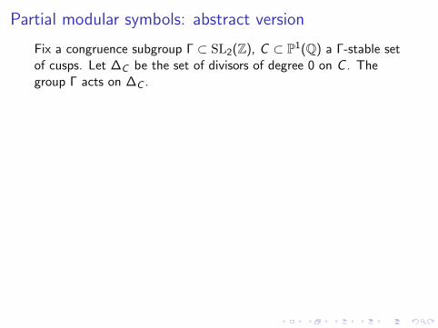
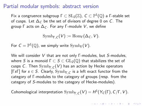
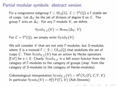
Fix a congruence subgroup Γ ⊂ SL2(Z), C ⊂ P1(Q) a Γ-stable setof cusps. Let ∆C be the set of divisors of degree 0 on C . Thegroup Γ acts on ∆C .
For any Γ-module V , we define
SymbΓ,C (V ) := HomΓ(∆C ,V ).
For C = P1(Q), we simply write SymbΓ(V ).
We will consider V that are not only Γ-modules, but S-modules,where S is a monoid Γ ⊂ S ⊂ GL2(Q) that stabilizes the set ofcusps C . Then SymbΓ,C (V ) has an action by Hecke operators[ΓsΓ] for s ∈ S . Clearly, SymbΓ,C is a left exact functor from thecategory of Γ-modules to the category of groups (resp. from thecategory of S-modules to the category of Hecke-modules).
Cohomological interpretation SymbΓ,C (V ) = H1(YC (Γ),C/Γ,V ).In particular SymbΓ(V ) = H1
c (Y (Γ),V ) (Ash-Stevens).
Partial modular symbols: abstract version
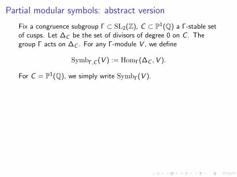
Fix a congruence subgroup Γ ⊂ SL2(Z), C ⊂ P1(Q) a Γ-stable setof cusps. Let ∆C be the set of divisors of degree 0 on C . Thegroup Γ acts on ∆C . For any Γ-module V , we define
SymbΓ,C (V ) := HomΓ(∆C ,V ).
For C = P1(Q), we simply write SymbΓ(V ).
We will consider V that are not only Γ-modules, but S-modules,where S is a monoid Γ ⊂ S ⊂ GL2(Q) that stabilizes the set ofcusps C . Then SymbΓ,C (V ) has an action by Hecke operators[ΓsΓ] for s ∈ S . Clearly, SymbΓ,C is a left exact functor from thecategory of Γ-modules to the category of groups (resp. from thecategory of S-modules to the category of Hecke-modules).
Cohomological interpretation SymbΓ,C (V ) = H1(YC (Γ),C/Γ,V ).In particular SymbΓ(V ) = H1
c (Y (Γ),V ) (Ash-Stevens).
Partial modular symbols: abstract version
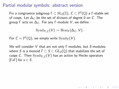
Fix a congruence subgroup Γ ⊂ SL2(Z), C ⊂ P1(Q) a Γ-stable setof cusps. Let ∆C be the set of divisors of degree 0 on C . Thegroup Γ acts on ∆C . For any Γ-module V , we define
SymbΓ,C (V ) := HomΓ(∆C ,V ).
For C = P1(Q), we simply write SymbΓ(V ).
We will consider V that are not only Γ-modules, but S-modules,where S is a monoid Γ ⊂ S ⊂ GL2(Q) that stabilizes the set ofcusps C . Then SymbΓ,C (V ) has an action by Hecke operators[ΓsΓ] for s ∈ S .
Clearly, SymbΓ,C is a left exact functor from thecategory of Γ-modules to the category of groups (resp. from thecategory of S-modules to the category of Hecke-modules).
Cohomological interpretation SymbΓ,C (V ) = H1(YC (Γ),C/Γ,V ).In particular SymbΓ(V ) = H1
c (Y (Γ),V ) (Ash-Stevens).
Partial modular symbols: abstract version
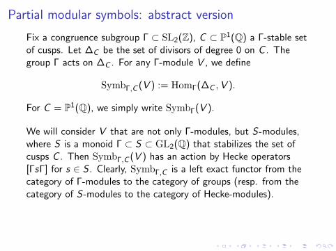
Fix a congruence subgroup Γ ⊂ SL2(Z), C ⊂ P1(Q) a Γ-stable setof cusps. Let ∆C be the set of divisors of degree 0 on C . Thegroup Γ acts on ∆C . For any Γ-module V , we define
SymbΓ,C (V ) := HomΓ(∆C ,V ).
For C = P1(Q), we simply write SymbΓ(V ).
We will consider V that are not only Γ-modules, but S-modules,where S is a monoid Γ ⊂ S ⊂ GL2(Q) that stabilizes the set ofcusps C . Then SymbΓ,C (V ) has an action by Hecke operators[ΓsΓ] for s ∈ S . Clearly, SymbΓ,C is a left exact functor from thecategory of Γ-modules to the category of groups (resp. from thecategory of S-modules to the category of Hecke-modules).
Cohomological interpretation SymbΓ,C (V ) = H1(YC (Γ),C/Γ,V ).In particular SymbΓ(V ) = H1
c (Y (Γ),V ) (Ash-Stevens).
Partial modular symbols: abstract version
Fix a congruence subgroup Γ ⊂ SL2(Z), C ⊂ P1(Q) a Γ-stable setof cusps. Let ∆C be the set of divisors of degree 0 on C . Thegroup Γ acts on ∆C . For any Γ-module V , we define
SymbΓ,C (V ) := HomΓ(∆C ,V ).
For C = P1(Q), we simply write SymbΓ(V ).
We will consider V that are not only Γ-modules, but S-modules,where S is a monoid Γ ⊂ S ⊂ GL2(Q) that stabilizes the set ofcusps C . Then SymbΓ,C (V ) has an action by Hecke operators[ΓsΓ] for s ∈ S . Clearly, SymbΓ,C is a left exact functor from thecategory of Γ-modules to the category of groups (resp. from thecategory of S-modules to the category of Hecke-modules).
Cohomological interpretation SymbΓ,C (V ) = H1(YC (Γ),C/Γ,V ).
In particular SymbΓ(V ) = H1c (Y (Γ),V ) (Ash-Stevens).
Partial modular symbols: abstract version
Fix a congruence subgroup Γ ⊂ SL2(Z), C ⊂ P1(Q) a Γ-stable setof cusps. Let ∆C be the set of divisors of degree 0 on C . Thegroup Γ acts on ∆C . For any Γ-module V , we define
SymbΓ,C (V ) := HomΓ(∆C ,V ).
For C = P1(Q), we simply write SymbΓ(V ).
We will consider V that are not only Γ-modules, but S-modules,where S is a monoid Γ ⊂ S ⊂ GL2(Q) that stabilizes the set ofcusps C . Then SymbΓ,C (V ) has an action by Hecke operators[ΓsΓ] for s ∈ S . Clearly, SymbΓ,C is a left exact functor from thecategory of Γ-modules to the category of groups (resp. from thecategory of S-modules to the category of Hecke-modules).
Cohomological interpretation SymbΓ,C (V ) = H1(YC (Γ),C/Γ,V ).In particular SymbΓ(V ) = H1
c (Y (Γ),V ) (Ash-Stevens).
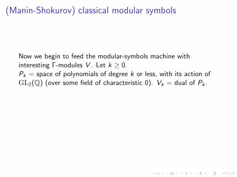
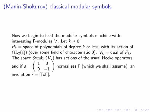
(Manin-Shokurov) classical modular symbols
Now we begin to feed the modular-symbols machine withinteresting Γ-modules V . Let k ≥ 0.Pk = space of polynomials of degree k or less, with its action ofGL2(Q) (over some field of characteristic 0). Vk = dual of Pk .
The space SymbΓ(Vk) has actions of the usual Hecke operators
and if s =
(1 00 −1
)normalizes Γ (which we shall assume), an
involution ι = [ΓsΓ].
(Manin-Shokurov) classical modular symbols
Now we begin to feed the modular-symbols machine withinteresting Γ-modules V . Let k ≥ 0.Pk = space of polynomials of degree k or less, with its action ofGL2(Q) (over some field of characteristic 0). Vk = dual of Pk .The space SymbΓ(Vk) has actions of the usual Hecke operators
and if s =
(1 00 −1
)normalizes Γ (which we shall assume), an
involution ι = [ΓsΓ].
Manin-Shokurov classical modular symbols
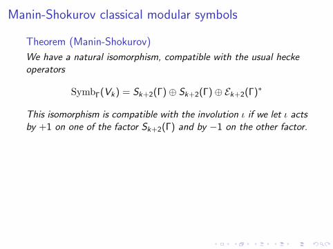
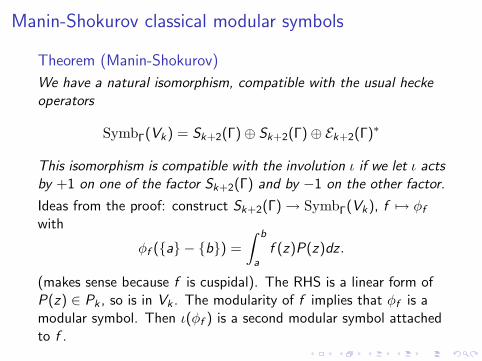
Theorem (Manin-Shokurov)
We have a natural isomorphism, compatible with the usual heckeoperators
SymbΓ(Vk) = Sk+2(Γ)⊕ Sk+2(Γ)⊕ Ek+2(Γ)∗
This isomorphism is compatible with the involution ι if we let ι actsby +1 on one of the factor Sk+2(Γ) and by −1 on the other factor.
Ideas from the proof: construct Sk+2(Γ)→ SymbΓ(Vk), f 7→ φf
with
φf ({a} − {b}) =
∫ b
af (z)P(z)dz .
(makes sense because f is cuspidal). The RHS is a linear form ofP(z) ∈ Pk , so is in Vk . The modularity of f implies that φf is amodular symbol. Then ι(φf ) is a second modular symbol attachedto f .
Manin-Shokurov classical modular symbols
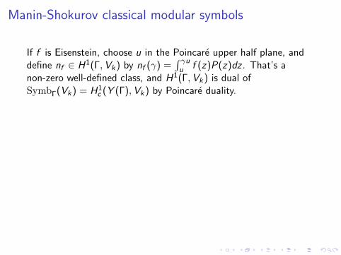
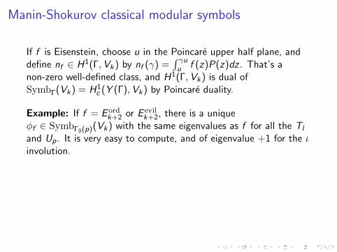
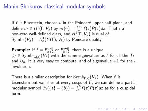
If f is Eisenstein, choose u in the Poincare upper half plane, anddefine nf ∈ H1(Γ,Vk) by nf (γ) =
∫ γuu f (z)P(z)dz . That’s a
non-zero well-defined class, and H1(Γ,Vk) is dual ofSymbΓ(Vk) = H1
c (Y (Γ),Vk) by Poincare duality.
Example: If f = E ordk+2 or E evil
k+2, there is a uniqueφf ∈ SymbΓ0(p)(Vk) with the same eigenvalues as f for all the Tl
and Up. It is very easy to compute, and of eigenvalue +1 for the ιinvolution.
There is a similar description for SymbΓ,C (Vk). When f isEisenstein but vanishes at every cusps of C , we can define a partialmodular symbol φ′f ({a} − {b}) =
∫ ba f (z)P(z)dz as for a cuspidal
form.
Manin-Shokurov classical modular symbols
If f is Eisenstein, choose u in the Poincare upper half plane, anddefine nf ∈ H1(Γ,Vk) by nf (γ) =
∫ γuu f (z)P(z)dz . That’s a
non-zero well-defined class, and H1(Γ,Vk) is dual ofSymbΓ(Vk) = H1
c (Y (Γ),Vk) by Poincare duality.
Example: If f = E ordk+2 or E evil
k+2, there is a uniqueφf ∈ SymbΓ0(p)(Vk) with the same eigenvalues as f for all the Tl
and Up. It is very easy to compute, and of eigenvalue +1 for the ιinvolution.
There is a similar description for SymbΓ,C (Vk). When f isEisenstein but vanishes at every cusps of C , we can define a partialmodular symbol φ′f ({a} − {b}) =
∫ ba f (z)P(z)dz as for a cuspidal
form.
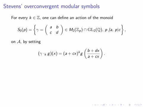
Stevens’ overconvergent modular symbols
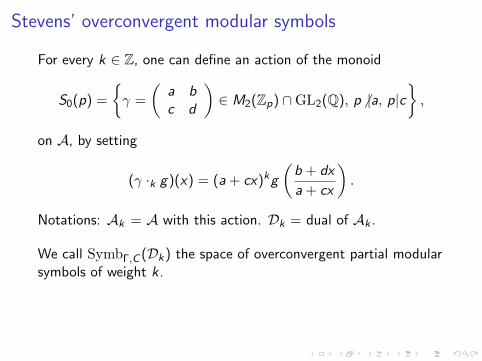
For every k ∈ Z, one can define an action of the monoid
S0(p) =
{γ =
(a bc d
)∈ M2(Zp) ∩GL2(Q), p 6 |a, p|c
},
on A, by setting
(γ ·k g)(x) = (a + cx)kg
(b + dx
a + cx
).
Notations: Ak = A with this action. Dk = dual of Ak .
We call SymbΓ,C (Dk) the space of overconvergent partial modularsymbols of weight k . Assume to fix ideas that Γ = Γ1(N) ∩ Γ0(p),and that C is either P1(Q) or the Γ-orbit of 0 and ∞. ThenSymbΓ,C (Dk) has an action of Tl for l prime to Np, Up, and theinvolution ι
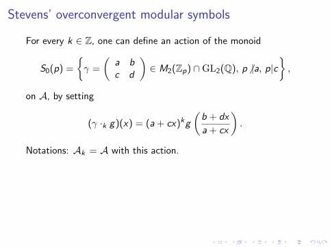
Stevens’ overconvergent modular symbols
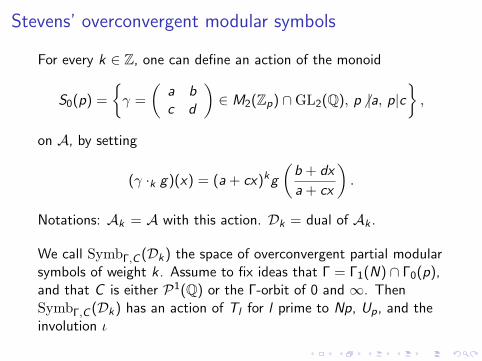
For every k ∈ Z, one can define an action of the monoid
S0(p) =
{γ =
(a bc d
)∈ M2(Zp) ∩GL2(Q), p 6 |a, p|c
},
on A, by setting
(γ ·k g)(x) = (a + cx)kg
(b + dx
a + cx
).
Notations: Ak = A with this action.
Dk = dual of Ak .
We call SymbΓ,C (Dk) the space of overconvergent partial modularsymbols of weight k . Assume to fix ideas that Γ = Γ1(N) ∩ Γ0(p),and that C is either P1(Q) or the Γ-orbit of 0 and ∞. ThenSymbΓ,C (Dk) has an action of Tl for l prime to Np, Up, and theinvolution ι
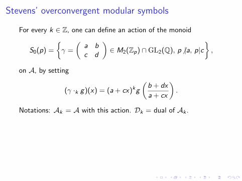
Stevens’ overconvergent modular symbols
For every k ∈ Z, one can define an action of the monoid
S0(p) =
{γ =
(a bc d
)∈ M2(Zp) ∩GL2(Q), p 6 |a, p|c
},
on A, by setting
(γ ·k g)(x) = (a + cx)kg
(b + dx
a + cx
).
Notations: Ak = A with this action. Dk = dual of Ak .
We call SymbΓ,C (Dk) the space of overconvergent partial modularsymbols of weight k . Assume to fix ideas that Γ = Γ1(N) ∩ Γ0(p),and that C is either P1(Q) or the Γ-orbit of 0 and ∞. ThenSymbΓ,C (Dk) has an action of Tl for l prime to Np, Up, and theinvolution ι
Stevens’ overconvergent modular symbols
For every k ∈ Z, one can define an action of the monoid
S0(p) =
{γ =
(a bc d
)∈ M2(Zp) ∩GL2(Q), p 6 |a, p|c
},
on A, by setting
(γ ·k g)(x) = (a + cx)kg
(b + dx
a + cx
).
Notations: Ak = A with this action. Dk = dual of Ak .
We call SymbΓ,C (Dk) the space of overconvergent partial modularsymbols of weight k .
Assume to fix ideas that Γ = Γ1(N) ∩ Γ0(p),and that C is either P1(Q) or the Γ-orbit of 0 and ∞. ThenSymbΓ,C (Dk) has an action of Tl for l prime to Np, Up, and theinvolution ι
Stevens’ overconvergent modular symbols
For every k ∈ Z, one can define an action of the monoid
S0(p) =
{γ =
(a bc d
)∈ M2(Zp) ∩GL2(Q), p 6 |a, p|c
},
on A, by setting
(γ ·k g)(x) = (a + cx)kg
(b + dx
a + cx
).
Notations: Ak = A with this action. Dk = dual of Ak .
We call SymbΓ,C (Dk) the space of overconvergent partial modularsymbols of weight k . Assume to fix ideas that Γ = Γ1(N) ∩ Γ0(p),and that C is either P1(Q) or the Γ-orbit of 0 and ∞. ThenSymbΓ,C (Dk) has an action of Tl for l prime to Np, Up, and theinvolution ι
Overconvergent vs classical modular symbols
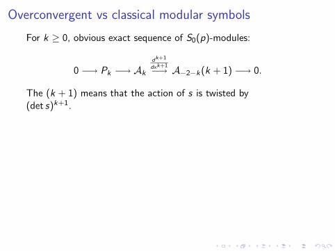
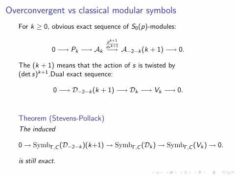
For k ≥ 0, obvious exact sequence of S0(p)-modules:
0 −→ Pk −→ Ak
dk+1
dxk+1−→ A−2−k(k + 1) −→ 0.
The (k + 1) means that the action of s is twisted by(det s)k+1.
Dual exact sequence:
0 −→ D−2−k(k + 1) −→ Dk −→ Vk −→ 0.
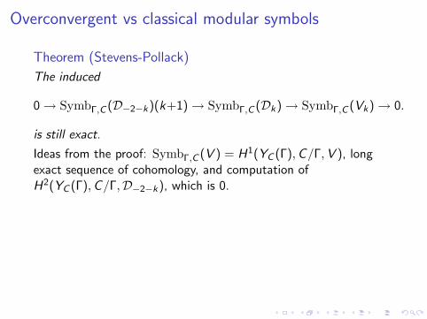
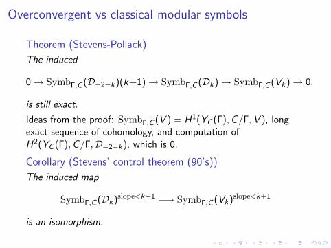
Theorem (Stevens-Pollack)
The induced
0→ SymbΓ,C (D−2−k)(k+1)→ SymbΓ,C (Dk)→ SymbΓ,C (Vk)→ 0.
is still exact.
Overconvergent vs classical modular symbols
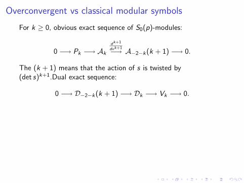
For k ≥ 0, obvious exact sequence of S0(p)-modules:
0 −→ Pk −→ Ak
dk+1
dxk+1−→ A−2−k(k + 1) −→ 0.
The (k + 1) means that the action of s is twisted by(det s)k+1.Dual exact sequence:
0 −→ D−2−k(k + 1) −→ Dk −→ Vk −→ 0.
Theorem (Stevens-Pollack)
The induced
0→ SymbΓ,C (D−2−k)(k+1)→ SymbΓ,C (Dk)→ SymbΓ,C (Vk)→ 0.
is still exact.
Overconvergent vs classical modular symbols
Theorem (Stevens-Pollack)
The induced
0→ SymbΓ,C (D−2−k)(k+1)→ SymbΓ,C (Dk)→ SymbΓ,C (Vk)→ 0.
is still exact.
Ideas from the proof: SymbΓ,C (V ) = H1(YC (Γ),C/Γ,V ), longexact sequence of cohomology, and computation ofH2(YC (Γ),C/Γ,D−2−k), which is 0.
Corollary (Stevens’ control theorem (90’s))
The induced map
SymbΓ,C (Dk)slope<k+1 −→ SymbΓ,C (Vk)slope<k+1
is an isomorphism.
Overview of the construction of the p-adic L-function inthe classical case
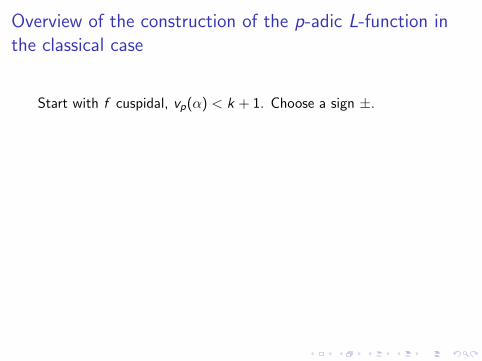
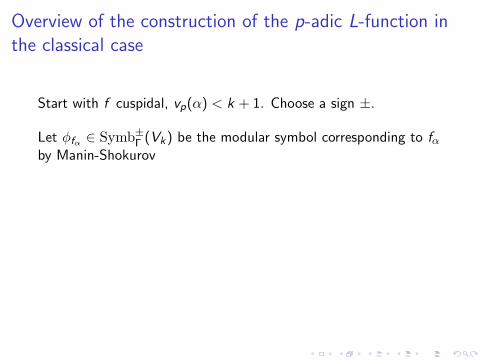
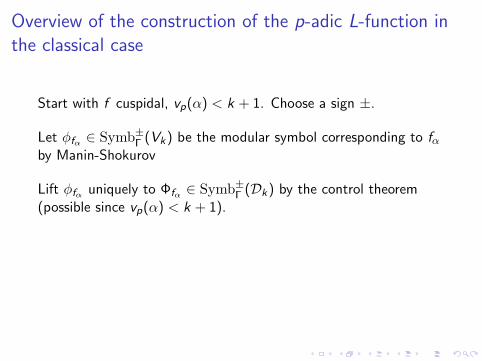
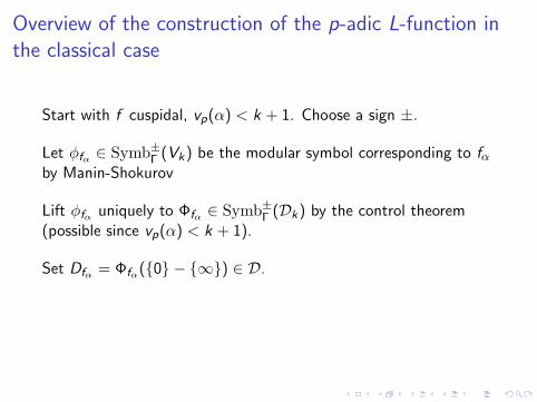
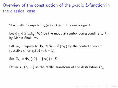
Start with f cuspidal, vp(α) < k + 1. Choose a sign ±.
Let φfα ∈ Symb±Γ (Vk) be the modular symbol corresponding to fαby Manin-Shokurov
Lift φfα uniquely to Φfα ∈ Symb±Γ (Dk) by the control theorem(possible since vp(α) < k + 1).
Set Dfα = Φfα({0} − {∞}) ∈ D.
Define L±p (fα,−) as the Mellin transform of the destribition Dfα .
Overview of the construction of the p-adic L-function inthe classical case
Start with f cuspidal, vp(α) < k + 1. Choose a sign ±.
Let φfα ∈ Symb±Γ (Vk) be the modular symbol corresponding to fαby Manin-Shokurov
Lift φfα uniquely to Φfα ∈ Symb±Γ (Dk) by the control theorem(possible since vp(α) < k + 1).
Set Dfα = Φfα({0} − {∞}) ∈ D.
Define L±p (fα,−) as the Mellin transform of the destribition Dfα .
Overview of the construction of the p-adic L-function inthe classical case
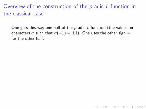
One gets this way one-half of the p-adic L-function (the values oncharacters σ such that σ(−1) = ±1). One uses the other sign ∓for the other half.
Proving the interpolation property is a simple computation usingthe way φfα is defined. The growth property results easily from Φfα
being an eigenform for Up of slope vp(α). Remark: nothingprevents us to apply the same method to an ordinary Eisensteinseries, e.g. E ord
k+2. Thus one can lift φEordk+2
uniquely to
ΦEordk+2∈ Symb+
Γ (Dk). But one finds that the distribution D+Eord
k+2
is
a derivative of a Dirac measure at 0, and its Mellin transform isthus 0. In this sense, the p-adic L-function of an ordinaryL-function is 0.
Overview of the construction of the p-adic L-function inthe classical case
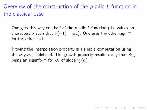
One gets this way one-half of the p-adic L-function (the values oncharacters σ such that σ(−1) = ±1). One uses the other sign ∓for the other half.
Proving the interpolation property is a simple computation usingthe way φfα is defined. The growth property results easily from Φfα
being an eigenform for Up of slope vp(α).
Remark: nothingprevents us to apply the same method to an ordinary Eisensteinseries, e.g. E ord
k+2. Thus one can lift φEordk+2
uniquely to
ΦEordk+2∈ Symb+
Γ (Dk). But one finds that the distribution D+Eord
k+2
is
a derivative of a Dirac measure at 0, and its Mellin transform isthus 0. In this sense, the p-adic L-function of an ordinaryL-function is 0.
Overview of the construction of the p-adic L-function inthe classical case
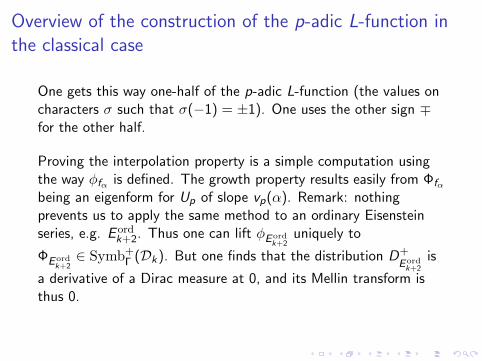
One gets this way one-half of the p-adic L-function (the values oncharacters σ such that σ(−1) = ±1). One uses the other sign ∓for the other half.
Proving the interpolation property is a simple computation usingthe way φfα is defined. The growth property results easily from Φfα
being an eigenform for Up of slope vp(α). Remark: nothingprevents us to apply the same method to an ordinary Eisensteinseries, e.g. E ord
k+2. Thus one can lift φEordk+2
uniquely to
ΦEordk+2∈ Symb+
Γ (Dk). But one finds that the distribution D+Eord
k+2
is
a derivative of a Dirac measure at 0, and its Mellin transform isthus 0.
In this sense, the p-adic L-function of an ordinaryL-function is 0.
Overview of the construction of the p-adic L-function inthe classical case
One gets this way one-half of the p-adic L-function (the values oncharacters σ such that σ(−1) = ±1). One uses the other sign ∓for the other half.
Proving the interpolation property is a simple computation usingthe way φfα is defined. The growth property results easily from Φfα
being an eigenform for Up of slope vp(α). Remark: nothingprevents us to apply the same method to an ordinary Eisensteinseries, e.g. E ord
k+2. Thus one can lift φEordk+2
uniquely to
ΦEordk+2∈ Symb+
Γ (Dk). But one finds that the distribution D+Eord
k+2
is
a derivative of a Dirac measure at 0, and its Mellin transform isthus 0. In this sense, the p-adic L-function of an ordinaryL-function is 0.
Overview of the construction of the p-adic L-functions inthe general case
Proposition (B.)
Assume that f is new, and that fα is cuspidal or evil Eisenstein.Then the eigenspace Symb±Γ [fα] has dimension 1.
Ideas: Construct the Stevens’ eigencurve for modular symbols,prove it is isomorphic to the Coleman-Mazur-Buzzard eigencurve,use results of Bellaiche-Chenevier that the eigencurve is smooth atclassical points.
Define Φ±fα as generators of those eigenspace, distributions
D±fα = Φ±fα({∞} − {0}) and the L-functions as Mellin transformsas above.
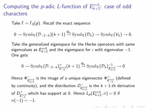
Computing the p-adic L-function of E evilk+2: case of odd
characters
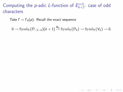
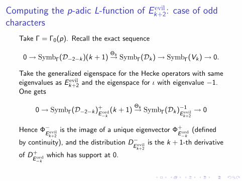
Take Γ = Γ0(p). Recall the exact sequence
0→ SymbΓ(D−2−k)(k + 1)Θk→ SymbΓ(Dk)→ SymbΓ(Vk)→ 0.
Take the generalized eigenspace for the Hecke operators with sameeigenvalues as E evil
k+2 and the eigenspace for ι with eigenvalue −1.One gets
0→ SymbΓ(D−2−k)+Eord−k
(k + 1)Θk→ SymbΓ(Dk)−1
Eevilk+2
→ 0
Hence Φ−Eevil
k+2
is the image of a unique eigenvector Φ+Eord−k
(defined
by continuity), and the distribution D−Eevil
k+2
is the k + 1-th derivative
of D+Eord−k
which has support at 0. Hence Lp(E evilk+2, σ) = 0 if
σ(−1) = −1.

Computing the p-adic L-function of E evilk+2: case of odd
characters
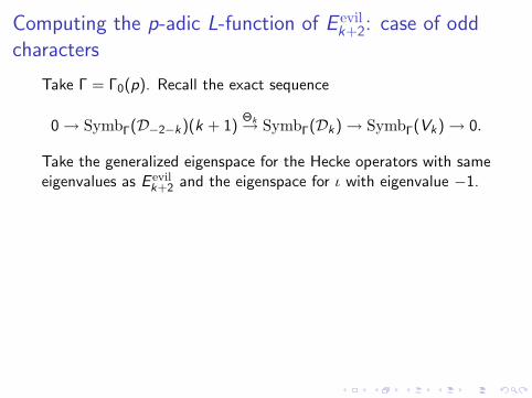
Take Γ = Γ0(p). Recall the exact sequence
0→ SymbΓ(D−2−k)(k + 1)Θk→ SymbΓ(Dk)→ SymbΓ(Vk)→ 0.
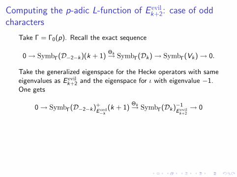
Take the generalized eigenspace for the Hecke operators with sameeigenvalues as E evil
k+2 and the eigenspace for ι with eigenvalue −1.
One gets
0→ SymbΓ(D−2−k)+Eord−k
(k + 1)Θk→ SymbΓ(Dk)−1
Eevilk+2
→ 0
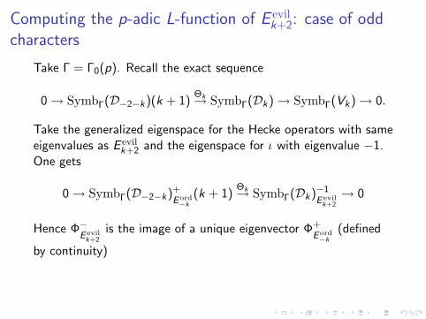
Hence Φ−Eevil
k+2
is the image of a unique eigenvector Φ+Eord−k
(defined
by continuity), and the distribution D−Eevil
k+2
is the k + 1-th derivative
of D+Eord−k
which has support at 0. Hence Lp(E evilk+2, σ) = 0 if
σ(−1) = −1.
Computing the p-adic L-function of E evilk+2: case of odd
characters
Take Γ = Γ0(p). Recall the exact sequence
0→ SymbΓ(D−2−k)(k + 1)Θk→ SymbΓ(Dk)→ SymbΓ(Vk)→ 0.
Take the generalized eigenspace for the Hecke operators with sameeigenvalues as E evil
k+2 and the eigenspace for ι with eigenvalue −1.
One gets
0→ SymbΓ(D−2−k)+Eord−k
(k + 1)Θk→ SymbΓ(Dk)−1
Eevilk+2
→ 0
Hence Φ−Eevil
k+2
is the image of a unique eigenvector Φ+Eord−k
(defined
by continuity), and the distribution D−Eevil
k+2
is the k + 1-th derivative
of D+Eord−k
which has support at 0. Hence Lp(E evilk+2, σ) = 0 if
σ(−1) = −1.
Computing the p-adic L-function of E evilk+2: case of odd
characters
Take Γ = Γ0(p). Recall the exact sequence
0→ SymbΓ(D−2−k)(k + 1)Θk→ SymbΓ(Dk)→ SymbΓ(Vk)→ 0.
Take the generalized eigenspace for the Hecke operators with sameeigenvalues as E evil
k+2 and the eigenspace for ι with eigenvalue −1.One gets
0→ SymbΓ(D−2−k)+Eord−k
(k + 1)Θk→ SymbΓ(Dk)−1
Eevilk+2
→ 0
Hence Φ−Eevil
k+2
is the image of a unique eigenvector Φ+Eord−k
(defined
by continuity), and the distribution D−Eevil
k+2
is the k + 1-th derivative
of D+Eord−k
which has support at 0. Hence Lp(E evilk+2, σ) = 0 if
σ(−1) = −1.
Computing the p-adic L-function of E evilk+2: case of odd
characters
Take Γ = Γ0(p). Recall the exact sequence
0→ SymbΓ(D−2−k)(k + 1)Θk→ SymbΓ(Dk)→ SymbΓ(Vk)→ 0.
Take the generalized eigenspace for the Hecke operators with sameeigenvalues as E evil
k+2 and the eigenspace for ι with eigenvalue −1.One gets
0→ SymbΓ(D−2−k)+Eord−k
(k + 1)Θk→ SymbΓ(Dk)−1
Eevilk+2
→ 0
Hence Φ−Eevil
k+2
is the image of a unique eigenvector Φ+Eord−k
(defined
by continuity)
, and the distribution D−Eevil
k+2
is the k + 1-th derivative
of D+Eord−k
which has support at 0. Hence Lp(E evilk+2, σ) = 0 if
σ(−1) = −1.
Computing the p-adic L-function of E evilk+2: case of odd
characters
Take Γ = Γ0(p). Recall the exact sequence
0→ SymbΓ(D−2−k)(k + 1)Θk→ SymbΓ(Dk)→ SymbΓ(Vk)→ 0.
Take the generalized eigenspace for the Hecke operators with sameeigenvalues as E evil
k+2 and the eigenspace for ι with eigenvalue −1.One gets
0→ SymbΓ(D−2−k)+Eord−k
(k + 1)Θk→ SymbΓ(Dk)−1
Eevilk+2
→ 0
Hence Φ−Eevil
k+2
is the image of a unique eigenvector Φ+Eord−k
(defined
by continuity), and the distribution D−Eevil
k+2
is the k + 1-th derivative
of D+Eord−k
which has support at 0.
Hence Lp(E evilk+2, σ) = 0 if
σ(−1) = −1.
Computing the p-adic L-function of E evilk+2: case of odd
characters
Take Γ = Γ0(p). Recall the exact sequence
0→ SymbΓ(D−2−k)(k + 1)Θk→ SymbΓ(Dk)→ SymbΓ(Vk)→ 0.
Take the generalized eigenspace for the Hecke operators with sameeigenvalues as E evil
k+2 and the eigenspace for ι with eigenvalue −1.One gets
0→ SymbΓ(D−2−k)+Eord−k
(k + 1)Θk→ SymbΓ(Dk)−1
Eevilk+2
→ 0
Hence Φ−Eevil
k+2
is the image of a unique eigenvector Φ+Eord−k
(defined
by continuity), and the distribution D−Eevil
k+2
is the k + 1-th derivative
of D+Eord−k
which has support at 0. Hence Lp(E evilk+2, σ) = 0 if
σ(−1) = −1.
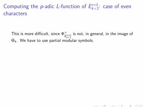
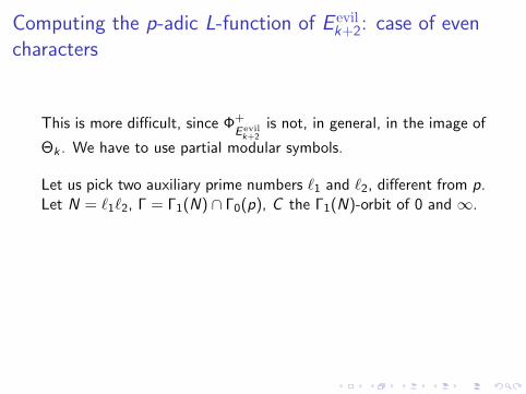
Computing the p-adic L-function of E evilk+2: case of even
characters
This is more difficult, since Φ+Eevil
k+2
is not, in general, in the image of
Θk . We have to use partial modular symbols.
Let us pick two auxiliary prime numbers `1 and `2, different from p.Let N = `1`2, Γ = Γ1(N) ∩ Γ0(p), C the Γ1(N)-orbit of 0 and ∞.
It is easy to see that we can pick fk+2 a linear combination ofEk+2(z), Ek+2(`1z), Ek+2(`2z) and Ek+2(`1`2z) which is regularat 0 and ∞, hence at every cusp of C . Let us also define f ord
k+2 by
the combination, with the same coefficients as fk+2, of E ordk+2
Computing the p-adic L-function of E evilk+2: case of even
characters (continued)
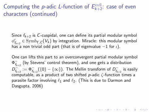
Since fk+2 is C -cuspidal, one can define its partial modular symbolφ′fk+2
∈ SymbΓ,C (Vk) by integration.
Miracle: this modular symbolhas a non trivial odd part (that is of eigenvalue −1 for ι).
One can lifts this part to an overconvergent partial modular symbolΦ−fk+2
(by Stevens’ control theorem), and one gets a distribution
D−fk+2:= Φ−fk+2
({0} − {∞}). The Mellin transform of D−fk+2is easily
computable, as a product of two shifted p-adic ζ-function times aparasite factor involving `1 and `2. (This is due to Darmon andDasgupta, 2006)
Computing the p-adic L-function of E evilk+2: case of even
characters (continued)
Since fk+2 is C -cuspidal, one can define its partial modular symbolφ′fk+2
∈ SymbΓ,C (Vk) by integration. Miracle: this modular symbolhas a non trivial odd part (that is of eigenvalue −1 for ι).
One can lifts this part to an overconvergent partial modular symbolΦ−fk+2
(by Stevens’ control theorem), and one gets a distribution
D−fk+2:= Φ−fk+2
({0} − {∞}).
The Mellin transform of D−fk+2is easily
computable, as a product of two shifted p-adic ζ-function times aparasite factor involving `1 and `2. (This is due to Darmon andDasgupta, 2006)
Computing the p-adic L-function of E evilk+2: case of even
characters (continued)
Since fk+2 is C -cuspidal, one can define its partial modular symbolφ′fk+2
∈ SymbΓ,C (Vk) by integration. Miracle: this modular symbolhas a non trivial odd part (that is of eigenvalue −1 for ι).
One can lifts this part to an overconvergent partial modular symbolΦ−fk+2
(by Stevens’ control theorem), and one gets a distribution
D−fk+2:= Φ−fk+2
({0} − {∞}). The Mellin transform of D−fk+2is easily
computable, as a product of two shifted p-adic ζ-function times aparasite factor involving `1 and `2. (This is due to Darmon andDasgupta, 2006)
Computing the p-adic L-function of E evilk+2: case of even
characters (continued)
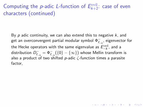
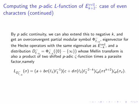
By p adic continuity, we can also extend this to negative k , andget an overconvergent partial modular symbol Φ−f−k
, eigenvector for
the Hecke operators with the same eigenvalue as E ord−k , and a
distribution D−f−k= Φ−f−k
({0} − {∞}) whose Mellin transform isalso a product of two shifted p-adic ζ-function times a parasitefactor,
namely
LD−f−k
(σ) = (a + bσ(`1)`−11 )(c + dσ(`2)`−2−k
2 )ζp(σtk+2)ζp(σz).
Computing the p-adic L-function of E evilk+2: case of even
characters (continued)
By p adic continuity, we can also extend this to negative k , andget an overconvergent partial modular symbol Φ−f−k
, eigenvector for
the Hecke operators with the same eigenvalue as E ord−k , and a
distribution D−f−k= Φ−f−k
({0} − {∞}) whose Mellin transform isalso a product of two shifted p-adic ζ-function times a parasitefactor,namely
LD−f−k
(σ) = (a + bσ(`1)`−11 )(c + dσ(`2)`−2−k
2 )ζp(σtk+2)ζp(σz).
Computing the p-adic L-function of E evilk+2: case of even
characters (continued)
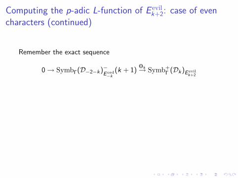
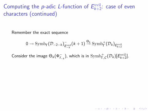
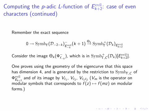
Remember the exact sequence
0→ SymbΓ(D−2−k)−Eord−k
(k + 1)Θk→ Symb+
Γ (Dk)Eevilk+2
Consider the image Θk(Φ−f−k), which is in Symb+
Γ,C (Dk)[E evilk+2].
One proves using the geometry of the eigencurve that this spacehas dimension 4, and is generated by the restriction to SymbΓ,C of
ΦevilEk+2
and of its image by V`1 , V`2 , V`1`2 (Vm is the operator onmodular symbols that corresponds to f (z) 7→ f (mz) on modularforms.)
Computing the p-adic L-function of E evilk+2: case of even
characters (continued)
Remember the exact sequence
0→ SymbΓ(D−2−k)−Eord−k
(k + 1)Θk→ Symb+
Γ (Dk)Eevilk+2
Consider the image Θk(Φ−f−k), which is in Symb+
Γ,C (Dk)[E evilk+2].
One proves using the geometry of the eigencurve that this spacehas dimension 4, and is generated by the restriction to SymbΓ,C of
ΦevilEk+2
and of its image by V`1 , V`2 , V`1`2 (Vm is the operator onmodular symbols that corresponds to f (z) 7→ f (mz) on modularforms.)
Computing the p-adic L-function of E evilk+2: case of even
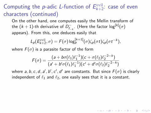
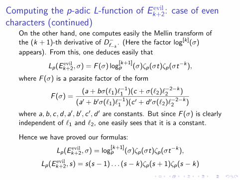
characters (continued)On the other hand, one computes easily the Mellin transform ofthe (k + 1)-th derivative of D−f−k
. (Here the factor log[k](σ)
appears). From this, one deduces easily that
Lp(E evilk+2, σ) = F (σ) log
[k+1]p (σ)ζp(σt)ζp(σt−k),
where F (σ) is a parasite factor of the form
F (σ) =(a + bσ(`1)`−1
1 )(c + σ(`2)`−2−k2 )
(a′ + b′σ(`1)`−11 )(c ′ + d ′σ(`2)`−2−k
2 )
where a, b, c , d , a′, b′, c ′, d ′ are constants. But since F (σ) is clearlyindependent of `1 and `2, one easily sees that it is a constant.
Hence we have proved our formulas:
Lp(E evilk+2, σ) = log
[k+1]p (σ)ζp(σt)ζp(σt−k),
Lp(E evilk+2, s) = s(s − 1) . . . (s − k)ζp(s + 1)ζp(s − k)
Computing the p-adic L-function of E evilk+2: case of even
characters (continued)On the other hand, one computes easily the Mellin transform ofthe (k + 1)-th derivative of D−f−k
. (Here the factor log[k](σ)
appears). From this, one deduces easily that
Lp(E evilk+2, σ) = F (σ) log
[k+1]p (σ)ζp(σt)ζp(σt−k),
where F (σ) is a parasite factor of the form
F (σ) =(a + bσ(`1)`−1
1 )(c + σ(`2)`−2−k2 )
(a′ + b′σ(`1)`−11 )(c ′ + d ′σ(`2)`−2−k
2 )
where a, b, c , d , a′, b′, c ′, d ′ are constants. But since F (σ) is clearlyindependent of `1 and `2, one easily sees that it is a constant.
Hence we have proved our formulas:
Lp(E evilk+2, σ) = log
[k+1]p (σ)ζp(σt)ζp(σt−k),
Lp(E evilk+2, s) = s(s − 1) . . . (s − k)ζp(s + 1)ζp(s − k)

![K arXiv:1109.4617v2 [math.NT] 24 Oct 2011 · 2018-11-02 · A FAMILY OF EISENSTEIN POLYNOMIALS GENERATING TOTALLY RAMIFIED EXTENSIONS, IDENTIFICATION OF EXTENSIONS AND CONSTRUCTION](https://static.fdocument.org/doc/165x107/5f381a048821ba3bfd131e45/k-arxiv11094617v2-mathnt-24-oct-2011-2018-11-02-a-family-of-eisenstein-polynomials.jpg)