The OPS-model Description of OPS 4.4.4 Ferd Sauter Hans van Jaarsveld Margreet van Zanten Eric van der Swaluw Jan Aben Frank de Leeuw National Institute for Public Health and the Environment (RIVM)

ops_v4_4_4_20150518a.docx, 2015-06-03 2

Changes with respect to previous description (v4.3.15) FS, 2012-11-14: chapter 3: added plot of Kz FS, 2012-11-15: chapter 6: rearranged text, added plot of τw and scavenging coefficient, changed eq.

6.10 FS, 2012-11-22: chapter 1: added section on receptors. FS, 2012-11-22: added appendix on substance-specific parameters (used to be part of the OPS

report Hans van Jaarsveld, 2004). FS, 2012-12-04: chapter 2: section 2.4.5 (wind profile) adapted to describe actual OPS code; figure

added. chapter 3: name of dimensional temperature gradient changed from Ψh to φh

chapter 5: stability correction in Ra better explained; figure added. FS, 2013-01-31: chapter 2: added graph for roughness correction of wind speeds in section

"Combining wind observations" FS, 2013-02-19: Table 2.4 Parameters calculated by the pre-processor METPRO added

motivation on different averaging types. FS, 2013-03-25: chapter 5: added choice of receptor height = 4 m (section on vertical gradient). FS, 2013-04-16: chapter 7: corrected the impression that ),( sxrn (NO2/NOx ratio, constant in space,

dependent on stability) is used for the NOy chemistry instead of rn,eff(x,s) (spatially variable).

FS, 2013-06-07: chapter 3: added documentation on Lagrangian time scale (Eq. 3.29, Figure 3.7). FS, 2013-06-12: chapter 3: added documentation on interpolation of σz in Figure 3.4 and section

"Procedure in OPS". FS, 2013-08-21: chapter 7: added yearly value of cr in Table 7.2. FS, 2013-09-12: chapter 5: slightly different notation for eq. 5.8, 5.9. FS, 2013-09-23: chapter 2: added note below table 2.2 about meaning of daily averaged

precipitation intensity. FS, 2013-11-05: changed formula (7.24) for kNH3 to actual implementation in OPS source code; this

kNH3 is approximately 1.8 times higher than the one of the previous documentation. Figure also adapted and added figure on source depletion factors.

FS, 2014-02-06: chapter 4: interchanged definition of daily variation code 4 and 5 for NH3 emissions.

FS, 2014-02-17: chapter 2, extended section 2.3.3. on precipitation characteristics. Table 2.2: unit of "length of rain events" changed from 0.01 h to 0.1 h.

FS, 2014-03-11: added sentences on yearly emission totals of NH3 emission after correction (section 4.3.3, 4.3.4).

FS, 2014-10-09: changed sentence on interpolation of precipitation parameters (section 2.3.2.3). FS, 2014-10-21: changed explanation of "The average length of a rain event" in section 2.3.3. FS, 2014-10-30/: added table with a summary of where background concentrations are used in the 2015-05-18 OPS-model. Added new plots of background maps. Also explained in more detail

how OPS deals with non-linearities (section 7.3). FS, 2014-04-16 added figure of canopy resistance for particles (section 5.4.3). JA, 2015-04-21 extended predefined daily emission variations for different categories of traffic

(section 4.1). JA, 2015-04-21 section on land use fractions instead of dominant land use. JA, 2015-05-04 changed section on particle size distributions (section 4.2). FS, 2015-05-12 changed the height where the wind speed is evaluated for plume rise calculations

(section 4.3.1). FS, 2015-05-18 changed description of creating roughness length maps (Table 5.3 and below). FS: Ferd Sauter JA: Jan Aben

2

ops_v4_4_4_20150518a.docx, 2015-06-03 3

Summary This report describes in detail OPS 4.4.4., a version of the OPS (Operational Priority Substances) model. OPS simulates the atmospheric process sequence of emission, dispersion, transport, chemical conversion and deposition. The main purpose of the model is to calculate the concentration and deposition of pollutants (e.g. particulate matter, acidifying compounds like SO2, NOx and NH3) for the Netherlands using a high spatial resolution (typical 1 x 1 km2). The model is, however, set up as a universal framework supporting the modelling of other pollutants such as fine particles and persistent organic pollutants. Previous versions of the model have been used since 1989 for atmospheric transport and deposition calculations published in the State of the Environment reports and Environmental Outlook studies in the Netherlands. Current versions are in use for the production of large-scale maps of air pollution in the Netherlands (RIVM 2011, Velders et al. 2011). This report is an update of the report Description and validation of OPS-Pro 4.1, RIVM report 500045001/2004 (van Jaarsveld, 2004). In this update, some processes have been described in more detail with explanatory figures. Furthermore, model changes, which have taken place since 2004, have been described. The main changes in the OPS-model are:

− a canopy compensation point has been included in the parameterisation of ammonia deposition (DEPAC module, van Zanten et al. 2010)

− a grid cell average is computed over multiple receptors inside a grid cell − area sources are subdivided into sub area sources for increased accuracy − inclusion of PM2.5 (extra particle class) − the roughness length is averaged over the whole trajectory; the roughness length map is

updated − background concentrations are updated (more recent years, future years, higher spatial

resolution). The various model validation exercises, described in van Jaarsveld (2004) are not repeated here. For further validation studies, the reader is referred to van Jaarsveld et al. (2005). A study on the dispersion of ammonia in an agricultural area is reported in van Pul et al. (2008). An intercomparison of measured and modelled ammonia concentrations in nature areas can be found in Stolk et al. (2009). A study on the influence of sea-salt particles on the exceedances of daily PM10 air quality standards is given in van Jaarsveld and Klimov (2011). A comparison between modelled and measured wet deposition levels of ammonium, nitrate and sulphate over the period 1992-2008 was reported in van der Swaluw et al. (2011).

3

ops_v4_4_4_20150518a.docx, 2015-06-03 4

Contents 1. Model description .............................................................................................................. 6

1.1 Introduction ................................................................................................................. 6 1.2 Substances ................................................................................................................... 6 1.3 Model characteristics................................................................................................... 7

1.3.1 Receptors.............................................................................................................. 9 1.3.2 Trajectories ........................................................................................................ 11 1.3.3 Vertical stratification ......................................................................................... 13 1.3.4 Classification with respect to the vertical structure of the boundary layer ........ 14

1.4 References ................................................................................................................. 15 2. Meteorological data ......................................................................................................... 17

2.1 Meteorological districts in the OPS model ............................................................... 17 2.2 Sources of primary meteorological data.................................................................... 18 2.3 Processing primary data (MPARKNMI)................................................................... 19

2.3.1 Calculating the potential wind speed ................................................................. 21 2.3.2 Spatial averaging of meteorological data ........................................................... 21 2.3.3 Calculation of precipitation characteristics ........................................................ 22 2.3.4 Determination of the snow cover indicator ........................................................ 23

2.4 The meteorological pre-processor (METPRO) ......................................................... 24 2.4.1 Cloud cover ........................................................................................................ 24 2.4.2 Derivation of boundary layer parameters .......................................................... 25 2.4.3 Pasquill classes................................................................................................... 26 2.4.4 Estimation of mixing heights ............................................................................. 27 2.4.5 The wind profile ................................................................................................. 28 2.4.6 Trajectories ........................................................................................................ 31 2.4.7 Summary of the meteorological data set ............................................................ 34

2.5 References ................................................................................................................. 35 2.6 Appendix: meteorological stations ............................................................................ 36

3. Mass balance and dispersion ............................................................................................ 38 3.1 Mass balance equations ............................................................................................. 38 3.2 Dispersion.................................................................................................................. 39 3.3 Vertical mixing close to sources ............................................................................... 40

3.3.1 Dispersion of heavy plumes ............................................................................... 41 3.3.2 Local vertical dispersion .................................................................................... 42

3.4 Area sources .............................................................................................................. 48 3.4.1 Horizontal dispersion for area sources ............................................................... 48 3.4.2 Vertical dispersion for area sources ................................................................... 50

3.5 References ................................................................................................................. 52 4. Emission and emission processes .................................................................................... 54

4.1 Emissions: behaviour in time .................................................................................... 54 4.2 Emission speciation ................................................................................................... 57 4.3 Emission processes .................................................................................................... 58

4.3.1 Plume rise........................................................................................................... 58 4.3.2 Inversion penetration ......................................................................................... 60 4.3.3 NH3 emissions from manure application ........................................................... 60 4.3.4 NH3 emissions from animal housing systems .................................................... 61

4.4 References ................................................................................................................. 62 5. Dry deposition .................................................................................................................. 63

5.1 Source depletion ........................................................................................................ 66 5.2 Source depletion for heavy plumes ........................................................................... 69

4

ops_v4_4_4_20150518a.docx, 2015-06-03 5

5.3 Non-acidifying substances ........................................................................................ 70 5.4 Acidifying and eutrophying substances .................................................................... 71

5.4.1 Dry deposition of gaseous substances................................................................ 71 5.4.2 Dry deposition of NOx ....................................................................................... 76 5.4.3 Dry deposition of acidifying aerosols ................................................................ 76 5.4.4 Dry deposition of NO3

- + HNO3 ........................................................................ 78 5.5 Appendix ................................................................................................................... 79

5.5.1 Derivation of the source depletion ratio for phase II of a plume ....................... 79 5.5.2 Derivation of the source depletion ratio for a heavy plume ............................... 81

5.6 References ................................................................................................................. 83 6. Wet deposition ................................................................................................................. 86

6.1 In-cloud scavenging .................................................................................................. 86 6.2 Below-cloud scavenging ........................................................................................... 87

6.2.1 Below-cloud scavenging of gases ...................................................................... 87 6.2.2 Below-cloud scavenging of particles ................................................................. 88

6.3 Effects of dry and wet periods on average scavenging rates..................................... 89 6.4 Combined in-cloud and below-cloud scavenging ..................................................... 91 6.5 Scavenging of reversibly soluble gases ..................................................................... 92 6.6 Overview of wet scavenging parameters .................................................................. 93 6.7 Verification and validation studies ............................................................................ 94 6.8 References ................................................................................................................. 94

7. Chemical transformation .................................................................................................. 96 7.1 Non-acidifying substances ........................................................................................ 96 7.2 Acidifying and eutrophying substances .................................................................... 97

7.2.1 Sulphur compounds ........................................................................................... 99 7.2.2 Nitrogen oxides ................................................................................................ 100 7.2.3 Ammonia compounds ...................................................................................... 105

7.3 Prescribed concentration levels (background concentrations) ................................ 107 7.4 Secondary species in OPS ....................................................................................... 111 7.5 References ............................................................................................................... 112

5

ops_v4_4_4_20150518a.docx, 2015-06-03 6

1. Model description

1.1 Introduction Modelling atmospheric processes has been the subject of many studies, resulting in a range of models with various complexities for specific applications. Before selecting a model or a model approach, we have to assess the intended application area carefully. In the present case, the time scale (long-range with a time resolution of a season or a few months) is probably the most important boundary condition. Another important condition is the spatial scale of the receptor area, which is defined as the Netherlands with a resolution of 5 x 5 km2 or 1 x 1 km2. The emission area, however, must be at least 2000 x 2000 km2 to explain the contribution of long-range transport to the levels of pollutants in the Netherlands. When OPS came into use (around 1985), these conditions forced exclusion of an Eulerian model framework, simply because of the required computer capacity. Furthermore, Eulerian models can suffer from large errors on a local scale, due to numerical dispersion. Eulerian models using nested grids should, to a certain extent, be applicable; however, operational models of this type were not available at that time. An efficient method for calculating long-term averages is arranging situations having similar properties into classes and then calculating representative concentrations for each of the classes. The average value will then follow from a summation of all concentrations, weighted with their relative frequencies of occurrence. Such a method is used for the OPS-model and is described in this chapter. One of the problems that arises from this approach is the choice of a good classification scheme on the basis of relevant parameters. For short-range models, a classification is usually made on the basis of wind direction, wind speed and atmospheric stability (see, for example Calder, 1971; Runca et al., 1982). As will be explained in more detail later on, OPS uses a classification based on transport distance, wind direction and a combination of atmospheric stability and mixing height. The approach used for the OPS-model, can be classified as a long-term climatological trajectory model which treats impacts of sources on a receptor independently. The model is basically a linear model. Because chemical conversion rates and dry deposition velocities depend on background concentrations taken from a series of concentration maps, one may call it a pseudo non-linear model. The physical background of the model concept and the derivation of relevant meteorological parameters from routine meteorological observations will be described in this chapter.

1.2 Substances The OPS model works with three groups of substances: 1. Acidifying and eutrophying substances (SO2, NOx, NH3 and secondary products). 2. Non-acidifying (gaseous) substances 3. Particle-bounded substances.

Acidifying and eutrophying substances Important environmental problems are the so-called acidification and eutrophication of ecosystems through the deposition of acidifying and eutrophying components. In this case a number of relevant processes have to be included in the model approach, since otherwise the model cannot adequately describe spatial differences and/or the development in time. Another reason for a special treatment of these components is the more than average availability of experimental data on emission, conversion and deposition processes. In OPS, the acidifying components include:

6

ops_v4_4_4_20150518a.docx, 2015-06-03 7

sulphur compounds (SOx) sulphur dioxide (SO2)

sulphate (SO42-)

oxidised nitrogen compounds (NOy) nitrogen oxides (NO and NO2) peroxyacetyl nitrate (PAN) nitrous acid (HNO2) nitric acid (HNO3) nitrate (NO3

-) reduced nitrogen compounds (NHy) ammonia (NH3)

ammonium (NH4+)

The gaseous SO2, NO and NH3 are primary emitted pollutants, while the gaseous NO2, PAN, HNO2 and HNO3 and the non-gaseous SO4

2-, NO3- and NH4

+ are formed from the primary pollutants in the atmosphere under influence of concentrations of, for example, ozone (O3) or free OH-radicals. In OPS, however, the primary oxidised nitrogen pollutant is defined as the sum of NO and NO2, further denoted as NOx. The secondary products SO4

2-, NO3- and NH4

+ form mainly ammonia salts having low vapour pressures and consequently appearing as aerosols in the atmosphere (Stelson and Seinfeld, 1982). Non-acidifying (gaseous) substances The group of non-acidifying substances uses a generic approach in which the properties of the substance are expressed in general terms such as:

- a chemical conversion/degradation rate - a dry deposition velocity or a surface resistance - a wet scavenging ratio.

Particle-bounded substances A generic approach is followed for substances attached to particles in which the size distribution of the particles fully defines the atmospheric behaviour.

1.3 Model characteristics The long-term OPS-LT model, which is outlined here, is a long-term Lagrangian transport and deposition model that describes relations between individual sources or source areas, and individual receptors by Gaussian plumes. The model is statistical in the sense that concentration and deposition values are calculated for a number of typical situations (classes) and the long-term value is obtained by summation of these values, weighted with their relative frequencies of occurrence. The short-term OPS-ST model is used on an hourly basis and computes hourly concentrations and depositions for a limited area (~ 0 - 50 km) only, using steady-state Gaussian plumes. The OPS-ST model will be described in a separate report. The description in this report is for the OPS-LT model, but many processes are modelled in OPS-ST in the same way. All equations governing the transport and deposition process are solved analytically, allowing the use of non-gridded receptors and sources, and variable grid sizes. OPS-LT assumes that transport from a source to a receptor takes place in straight, well-mixed sectors of height zi and horizontal angles of 30° (see Figure 1.1).

7

ops_v4_4_4_20150518a.docx, 2015-06-03 8

15

145

2

753

105

4

135

5

165

6

195

7225

8

255 9

285

10

315

11

345

12

North

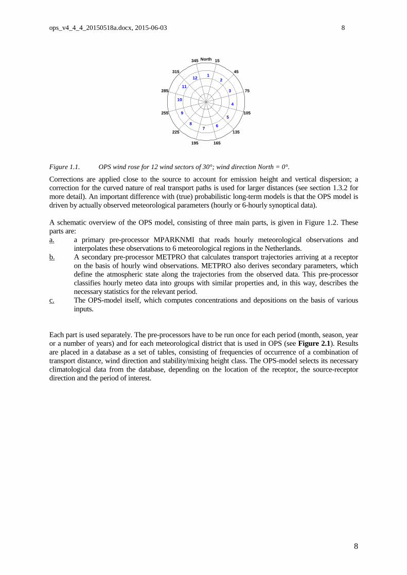
Figure 1.1. OPS wind rose for 12 wind sectors of 30°; wind direction North = 0°.

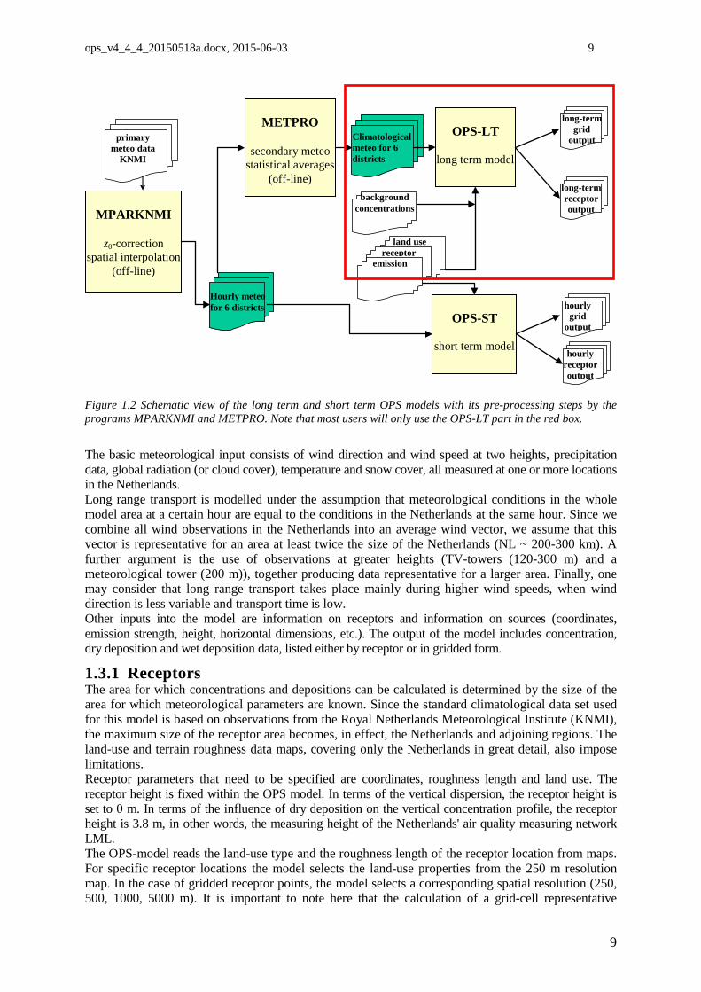
Corrections are applied close to the source to account for emission height and vertical dispersion; a correction for the curved nature of real transport paths is used for larger distances (see section 1.3.2 for more detail). An important difference with (true) probabilistic long-term models is that the OPS model is driven by actually observed meteorological parameters (hourly or 6-hourly synoptical data). A schematic overview of the OPS model, consisting of three main parts, is given in Figure 1.2. These parts are: a. a primary pre-processor MPARKNMI that reads hourly meteorological observations and

interpolates these observations to 6 meteorological regions in the Netherlands. b. A secondary pre-processor METPRO that calculates transport trajectories arriving at a receptor

on the basis of hourly wind observations. METPRO also derives secondary parameters, which define the atmospheric state along the trajectories from the observed data. This pre-processor classifies hourly meteo data into groups with similar properties and, in this way, describes the necessary statistics for the relevant period.

c. The OPS-model itself, which computes concentrations and depositions on the basis of various inputs.

Each part is used separately. The pre-processors have to be run once for each period (month, season, year or a number of years) and for each meteorological district that is used in OPS (see Figure 2.1). Results are placed in a database as a set of tables, consisting of frequencies of occurrence of a combination of transport distance, wind direction and stability/mixing height class. The OPS-model selects its necessary climatological data from the database, depending on the location of the receptor, the source-receptor direction and the period of interest.

8

ops_v4_4_4_20150518a.docx, 2015-06-03 9

Figure 1.2 Schematic view of the long term and short term OPS models with its pre-processing steps by the programs MPARKNMI and METPRO. Note that most users will only use the OPS-LT part in the red box.

The basic meteorological input consists of wind direction and wind speed at two heights, precipitation data, global radiation (or cloud cover), temperature and snow cover, all measured at one or more locations in the Netherlands. Long range transport is modelled under the assumption that meteorological conditions in the whole model area at a certain hour are equal to the conditions in the Netherlands at the same hour. Since we combine all wind observations in the Netherlands into an average wind vector, we assume that this vector is representative for an area at least twice the size of the Netherlands (NL ~ 200-300 km). A further argument is the use of observations at greater heights (TV-towers (120-300 m) and a meteorological tower (200 m)), together producing data representative for a larger area. Finally, one may consider that long range transport takes place mainly during higher wind speeds, when wind direction is less variable and transport time is low. Other inputs into the model are information on receptors and information on sources (coordinates, emission strength, height, horizontal dimensions, etc.). The output of the model includes concentration, dry deposition and wet deposition data, listed either by receptor or in gridded form.

1.3.1 Receptors The area for which concentrations and depositions can be calculated is determined by the size of the area for which meteorological parameters are known. Since the standard climatological data set used for this model is based on observations from the Royal Netherlands Meteorological Institute (KNMI), the maximum size of the receptor area becomes, in effect, the Netherlands and adjoining regions. The land-use and terrain roughness data maps, covering only the Netherlands in great detail, also impose limitations. Receptor parameters that need to be specified are coordinates, roughness length and land use. The receptor height is fixed within the OPS model. In terms of the vertical dispersion, the receptor height is set to 0 m. In terms of the influence of dry deposition on the vertical concentration profile, the receptor height is 3.8 m, in other words, the measuring height of the Netherlands' air quality measuring network LML. The OPS-model reads the land-use type and the roughness length of the receptor location from maps. For specific receptor locations the model selects the land-use properties from the 250 m resolution map. In the case of gridded receptor points, the model selects a corresponding spatial resolution (250, 500, 1000, 5000 m). It is important to note here that the calculation of a grid-cell representative

OPS-LT

long term model

Hourly meteo for 6 districts

Climatological meteo for 6 districts

METPRO

secondary meteo

statistical averages (off-line)

OPS-ST

short term model

primary meteo data

KNMI

MPARKNMI

z0-correction

spatial interpolation (off-line)

long-term grid

output

long-term receptor output

hourly grid

output

hourly receptor output

land use receptor

emission

background concentrations

9

ops_v4_4_4_20150518a.docx, 2015-06-03 10

roughness length is based on a logarithmic weighing of roughness elements, while the grid cell representative land-use type is defined as the most abundant land-use type within that grid cell. This model does not explicitly take into account the direct influence of obstacles (e.g. buildings) on the dispersion. Instead, the general influence of obstacles is expressed in the terrain roughness variable, assuming that obstacles are homogeneously distributed over the emission-receptor area. The shortest source-receptor distance for which this model may be used is therefore taken as a function of the terrain roughness length. In flat terrain with no obstacles the minimum distance is in the order of 20 m. For a terrain roughness > 0.1 m, the shortest distance is approx. 200 times the roughness length. When the stack is part of a building, the shortest distance is at least five times the height of the building. The model generates no warnings if these rules are violated. One should be aware that in the case of gridded receptor points in combination with point sources, the minimum source-receptor distance requirement cannot always be met. Receptor points for calculating concentrations and depositions can be chosen:

♦ on a regular (Cartesian) grid, with a grid distance to be chosen. The domain may be pre-defined (the Netherlands) or defined by the user.

♦ for a number of specific locations to be defined by the user. The output format differs according to the option chosen. The latter option is especially useful when results have to be compared with observations. The gridded results are formatted in a matrix form, while the results for specific receptor points are formatted as single records for each point. When the user selects grid output, OPS automatically generates multiple sub-receptors inside a grid cell in order to be able to compute a representative grid cell average. The number of sub-receptors goes to 1 with increasing source-receptor distance.

10

ops_v4_4_4_20150518a.docx, 2015-06-03 11

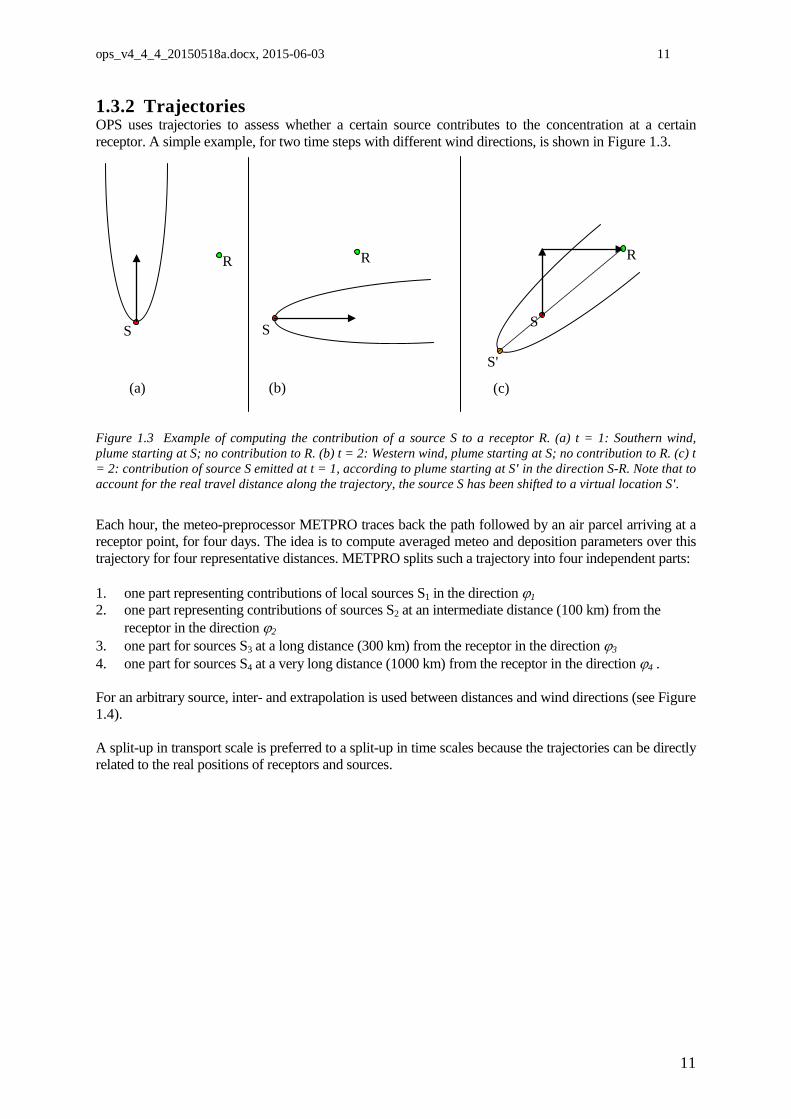
1.3.2 Trajectories OPS uses trajectories to assess whether a certain source contributes to the concentration at a certain receptor. A simple example, for two time steps with different wind directions, is shown in Figure 1.3.

Figure 1.3 Example of computing the contribution of a source S to a receptor R. (a) t = 1: Southern wind, plume starting at S; no contribution to R. (b) t = 2: Western wind, plume starting at S; no contribution to R. (c) t = 2: contribution of source S emitted at t = 1, according to plume starting at S' in the direction S-R. Note that to account for the real travel distance along the trajectory, the source S has been shifted to a virtual location S'.

Each hour, the meteo-preprocessor METPRO traces back the path followed by an air parcel arriving at a receptor point, for four days. The idea is to compute averaged meteo and deposition parameters over this trajectory for four representative distances. METPRO splits such a trajectory into four independent parts: 1. one part representing contributions of local sources S1 in the direction ϕ1 2. one part representing contributions of sources S2 at an intermediate distance (100 km) from the

receptor in the direction ϕ2 3. one part for sources S3 at a long distance (300 km) from the receptor in the direction ϕ3 4. one part for sources S4 at a very long distance (1000 km) from the receptor in the direction ϕ4 . For an arbitrary source, inter- and extrapolation is used between distances and wind directions (see Figure 1.4). A split-up in transport scale is preferred to a split-up in time scales because the trajectories can be directly related to the real positions of receptors and sources.

(a) (b) (c)

S

R

S'

S

R

S

R

11

ops_v4_4_4_20150518a.docx, 2015-06-03 12

Figure 1.4 Classification of trajectories in terms of source−receptor distance and source−receptor direction.

Receptor R located in the origin. METPRO characterises representative sources Si (i = 1,4) by transport distance di (= 0, 100, 300, 1000 km) and source-receptor angle φi (angle between North and dashed line). Note that φi is the angle of the average of all wind vectors between Si and R. For a source S as shown here, OPS interpolates all relevant parameters between classes corresponding with distances d3 and d4 and angles φ3 and φ4 .

The local scale represents situations where changes in meteorological conditions during transport are assumed to play no important role. This is usually within 1 or 2 hours after a substance is released into the atmosphere or within 20 km from the point of release. The 1000 km trajectory represents the long-range transport of pollutants with 2-4 days transport time. For most substances the contribution of sources in this range is only 5-10 % (for Western Europe). Statistical properties of trajectories (direction, speed, height) in this range appear to be less sensitive to trajectory lengths, so the properties of these trajectories are also used for transport distances greater than 1000 km. The trajectory of 300 km long is chosen such that it covers a full diurnal cycle in meteorological parameters, of which the mixing height is the most important. The 100-km trajectory represents transport on a sub-diurnal time scale as an intermediate between the local-and regional-scale transport. Within the 100 km trajectory, transitions in atmospheric stability and mixing height due to night-day transitions occur frequently. To describe the transport from a source located in a certain wind sector, average properties for all trajectories passing the source area are introduced. An important parameter is the effective path ratio, fpeff, which is calculated for all four distances considered. This parameter represents the ratio between the length of the (curved) path, xpath, followed by an air parcel and the straight source-receptor distance xsr : fpeff = xpath / xsr . (1.1)

S2

S4

180°

270° 90° R

S1 S3

S

300 km

100 km

0° 1000 km

12

ops_v4_4_4_20150518a.docx, 2015-06-03 13

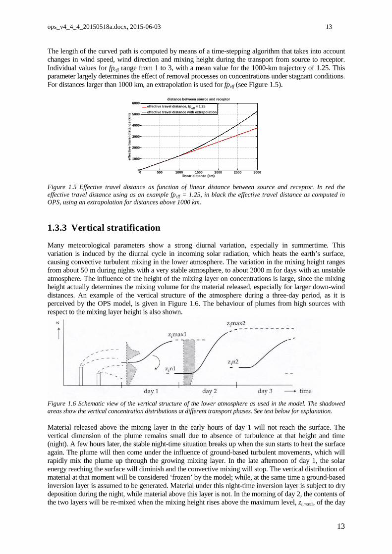
The length of the curved path is computed by means of a time-stepping algorithm that takes into account changes in wind speed, wind direction and mixing height during the transport from source to receptor. Individual values for fpeff range from 1 to 3, with a mean value for the 1000-km trajectory of 1.25. This parameter largely determines the effect of removal processes on concentrations under stagnant conditions. For distances larger than 1000 km, an extrapolation is used for fpeff (see Figure 1.5).

0 500 1000 1500 2000 2500 30000

1000

2000

3000

4000

5000

6000distance between source and receptor

linear distance (km)

effe

ctiv

e tr

avel

dis

tanc

e (k

m)

effective travel distance, fpeff = 1.25effective travel distance with extrapolation

Figure 1.5 Effective travel distance as function of linear distance between source and receptor. In red the effective travel distance using as an example fpeff = 1.25, in black the effective travel distance as computed in OPS, using an extrapolation for distances above 1000 km.

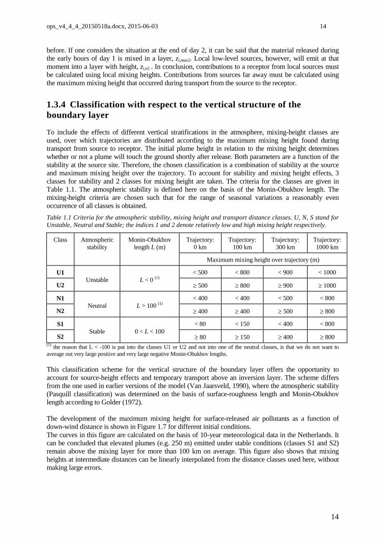
1.3.3 Vertical stratification Many meteorological parameters show a strong diurnal variation, especially in summertime. This variation is induced by the diurnal cycle in incoming solar radiation, which heats the earth’s surface, causing convective turbulent mixing in the lower atmosphere. The variation in the mixing height ranges from about 50 m during nights with a very stable atmosphere, to about 2000 m for days with an unstable atmosphere. The influence of the height of the mixing layer on concentrations is large, since the mixing height actually determines the mixing volume for the material released, especially for larger down-wind distances. An example of the vertical structure of the atmosphere during a three-day period, as it is perceived by the OPS model, is given in Figure 1.6. The behaviour of plumes from high sources with respect to the mixing layer height is also shown.

Figure 1.6 Schematic view of the vertical structure of the lower atmosphere as used in the model. The shadowed areas show the vertical concentration distributions at different transport phases. See text below for explanation. Material released above the mixing layer in the early hours of day 1 will not reach the surface. The vertical dimension of the plume remains small due to absence of turbulence at that height and time (night). A few hours later, the stable night-time situation breaks up when the sun starts to heat the surface again. The plume will then come under the influence of ground-based turbulent movements, which will rapidly mix the plume up through the growing mixing layer. In the late afternoon of day 1, the solar energy reaching the surface will diminish and the convective mixing will stop. The vertical distribution of material at that moment will be considered ‘frozen’ by the model; while, at the same time a ground-based inversion layer is assumed to be generated. Material under this night-time inversion layer is subject to dry deposition during the night, while material above this layer is not. In the morning of day 2, the contents of the two layers will be re-mixed when the mixing height rises above the maximum level, zi,max1, of the day

13

ops_v4_4_4_20150518a.docx, 2015-06-03 14

before. If one considers the situation at the end of day 2, it can be said that the material released during the early hours of day 1 is mixed in a layer, zi,max2. Local low-level sources, however, will emit at that moment into a layer with height, zi,n2 . In conclusion, contributions to a receptor from local sources must be calculated using local mixing heights. Contributions from sources far away must be calculated using the maximum mixing height that occurred during transport from the source to the receptor.

1.3.4 Classification with respect to the vertical structure of the boundary layer To include the effects of different vertical stratifications in the atmosphere, mixing-height classes are used, over which trajectories are distributed according to the maximum mixing height found during transport from source to receptor. The initial plume height in relation to the mixing height determines whether or not a plume will touch the ground shortly after release. Both parameters are a function of the stability at the source site. Therefore, the chosen classification is a combination of stability at the source and maximum mixing height over the trajectory. To account for stability and mixing height effects, 3 classes for stability and 2 classes for mixing height are taken. The criteria for the classes are given in Table 1.1. The atmospheric stability is defined here on the basis of the Monin-Obukhov length. The mixing-height criteria are chosen such that for the range of seasonal variations a reasonably even occurrence of all classes is obtained. Table 1.1 Criteria for the atmospheric stability, mixing height and transport distance classes. U, N, S stand for Unstable, Neutral and Stable; the indices 1 and 2 denote relatively low and high mixing height respectively.

Class Atmospheric stability

Monin-Obukhov length L (m)

Trajectory: 0 km

Trajectory: 100 km

Trajectory: 300 km

Trajectory: 1000 km

Maximum mixing height over trajectory (m)

U1 Unstable L < 0 (1)

< 500 < 800 < 900 < 1000

U2 ≥ 500 ≥ 800 ≥ 900 ≥ 1000

N1 Neutral L > 100 (1)

< 400 < 400 < 500 < 800

N2 ≥ 400 ≥ 400 ≥ 500 ≥ 800

S1 Stable 0 < L < 100

< 80 < 150 < 400 < 800

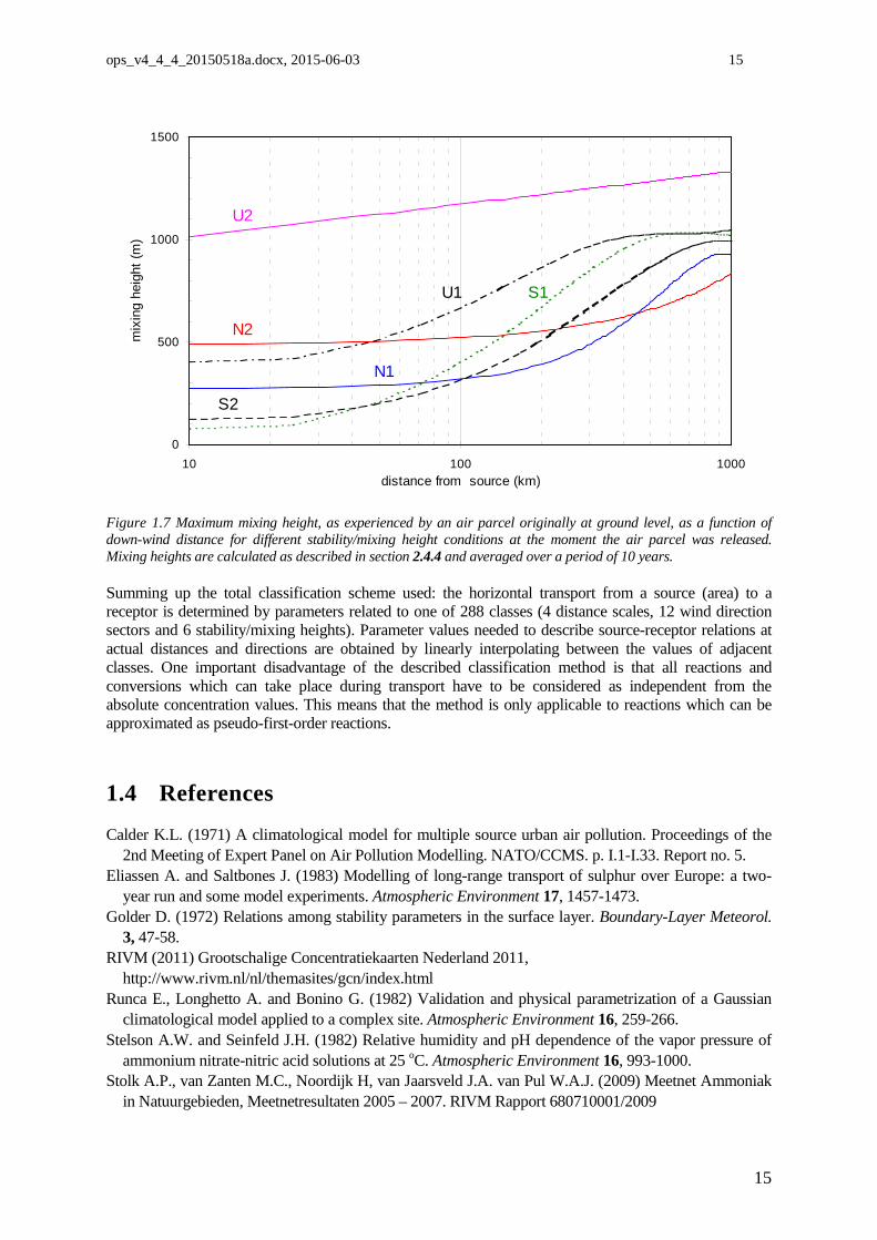
S2 ≥ 80 ≥ 150 ≥ 400 ≥ 800 (1) the reason that L < -100 is put into the classes U1 or U2 and not into one of the neutral classes, is that we do not want to average out very large positive and very large negative Monin-Obukhov lengths. This classification scheme for the vertical structure of the boundary layer offers the opportunity to account for source-height effects and temporary transport above an inversion layer. The scheme differs from the one used in earlier versions of the model (Van Jaarsveld, 1990), where the atmospheric stability (Pasquill classification) was determined on the basis of surface-roughness length and Monin-Obukhov length according to Golder (1972). The development of the maximum mixing height for surface-released air pollutants as a function of down-wind distance is shown in Figure 1.7 for different initial conditions. The curves in this figure are calculated on the basis of 10-year meteorological data in the Netherlands. It can be concluded that elevated plumes (e.g. 250 m) emitted under stable conditions (classes S1 and S2) remain above the mixing layer for more than 100 km on average. This figure also shows that mixing heights at intermediate distances can be linearly interpolated from the distance classes used here, without making large errors.

14

ops_v4_4_4_20150518a.docx, 2015-06-03 15

0

500

1000

1500

10 100 1000distance from source (km)

mix

ing

heig

ht (m

)

U2

N2

U1 S1

N1

S2

Figure 1.7 Maximum mixing height, as experienced by an air parcel originally at ground level, as a function of down-wind distance for different stability/mixing height conditions at the moment the air parcel was released. Mixing heights are calculated as described in section 2.4.4 and averaged over a period of 10 years. Summing up the total classification scheme used: the horizontal transport from a source (area) to a receptor is determined by parameters related to one of 288 classes (4 distance scales, 12 wind direction sectors and 6 stability/mixing heights). Parameter values needed to describe source-receptor relations at actual distances and directions are obtained by linearly interpolating between the values of adjacent classes. One important disadvantage of the described classification method is that all reactions and conversions which can take place during transport have to be considered as independent from the absolute concentration values. This means that the method is only applicable to reactions which can be approximated as pseudo-first-order reactions.

1.4 References Calder K.L. (1971) A climatological model for multiple source urban air pollution. Proceedings of the

2nd Meeting of Expert Panel on Air Pollution Modelling. NATO/CCMS. p. I.1-I.33. Report no. 5. Eliassen A. and Saltbones J. (1983) Modelling of long-range transport of sulphur over Europe: a two-

year run and some model experiments. Atmospheric Environment 17, 1457-1473. Golder D. (1972) Relations among stability parameters in the surface layer. Boundary-Layer Meteorol.

3, 47-58. RIVM (2011) Grootschalige Concentratiekaarten Nederland 2011, http://www.rivm.nl/nl/themasites/gcn/index.html Runca E., Longhetto A. and Bonino G. (1982) Validation and physical parametrization of a Gaussian

climatological model applied to a complex site. Atmospheric Environment 16, 259-266. Stelson A.W. and Seinfeld J.H. (1982) Relative humidity and pH dependence of the vapor pressure of

ammonium nitrate-nitric acid solutions at 25 oC. Atmospheric Environment 16, 993-1000. Stolk A.P., van Zanten M.C., Noordijk H, van Jaarsveld J.A. van Pul W.A.J. (2009) Meetnet Ammoniak

in Natuurgebieden, Meetnetresultaten 2005 – 2007. RIVM Rapport 680710001/2009

15

ops_v4_4_4_20150518a.docx, 2015-06-03 16

Van der Swaluw, Eric, Asman, Willem A.H., van Jaarsveld, Hans, Hoogerbrugge, Ronald (2011) Wet deposition of ammonium, nitrate and sulfate in the Netherlands over the period 1992–2008, Atmospheric Environment, 45, 3819-3826, 10.1016/j.atmosenv.2011.04.017.

Van Jaarsveld J.A. (1990) An operational atmospheric transport model for priority substances; specification and instructions for use. RIVM, Bilthoven, the Netherlands. Report no. 222501002.

Van Jaarsveld J.A. (2004) Description and validation of OPS-Pro 4.1, RIVM report 500045001/2004. Van Jaarsveld, H., Velders G. and Van Pul A. (2005) Evaluation and validation of the OPS multi-

scale model using local, national and international datasets. 10th Int. Conf. on Harmonisation of Atmospheric Dispersion models for Regulatory Purposes; 17-20 oktober 2005, Sissi, Kreta

Van Jaarsveld J.A. and D. Klimov (2011) Modelling the impact of sea-salt particles on the exceedances of daily PM10 air quality standards in the Netherlands. Int. J. Environment and Pollution, Vol. 44, Nos. 1/2/3/4, 2011

Van Pul, W.A.J., J.A. van Jaarsveld, O.S. Vellinga, M.van den Broek, M.C.J. Smits (2008) The VELD experiment: An evaluation of the ammonia emissions and concentrations in an agricultural area. Atmospheric Environment, 42, 8086-8095

Van Zanten, M.C., F.J. Sauter, R.J. Wichink Kruit, J.A. van Jaarsveld, W.A.J. van Pul (2010) Description of the DEPAC module. Dry deposition modelling with DEPAC_GCN2010. RIVM report 680180001

Velders G.J.M, Aben J.M.M., Jimmink B.A., van der Swaluw E., de Vries W.J. (2011) Grootschalige concentratie- en depositiekaarten Nederland. Rapportage 2011, RIVM report 680362001.

16

ops_v4_4_4_20150518a.docx, 2015-06-03

17

2. Meteorological data Air pollution modelling relies heavily on meteorological input data. Processes such as plume rise, dilution, dispersion and long-range transport depend not only on wind speed but also on turbulence characteristics and on the wind field over the area where the pollutant is dispersed. Although parameters such as turbulence may be measured directly in the field, it is not very practical and certainly very expensive. Therefore, most model approaches make a distinction between real observations of primary data (wind, temperature, radiation etceteras) and secondary parameters (friction velocity, Monin-Obukhov length, mixing height etceteras), derived from the set of primary parameters. The OPS model is designed to make use of standard and routinely available meteorological data. The parameters are wind speed and wind direction at two heights, temperature, global radiation, precipitation, snow cover and relative humidity.

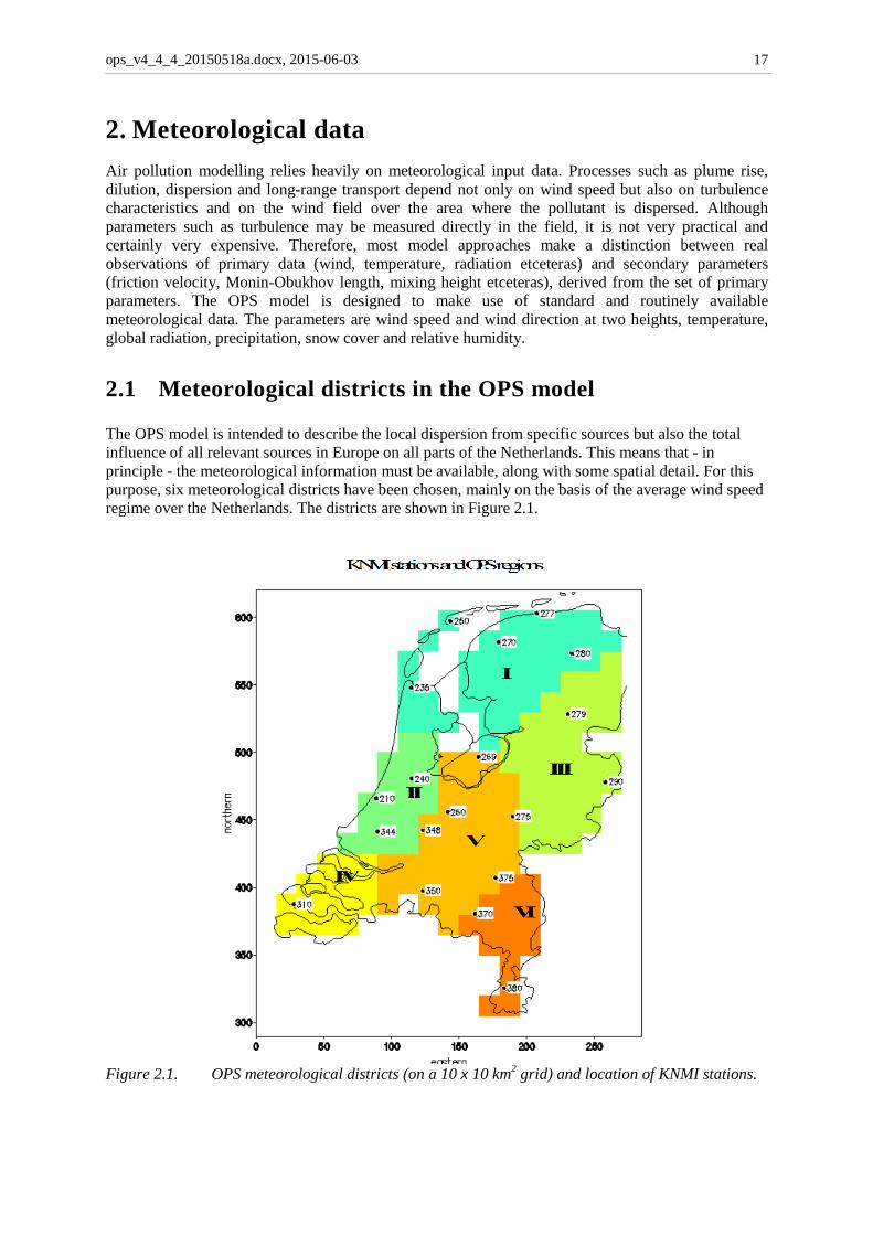
2.1 Meteorological districts in the OPS model The OPS model is intended to describe the local dispersion from specific sources but also the total influence of all relevant sources in Europe on all parts of the Netherlands. This means that - in principle - the meteorological information must be available, along with some spatial detail. For this purpose, six meteorological districts have been chosen, mainly on the basis of the average wind speed regime over the Netherlands. The districts are shown in Figure 2.1.

Figure 2.1. OPS meteorological districts (on a 10 x 10 km2 grid) and location of KNMI stations.

ops_v4_4_4_20150518a.docx, 2015-06-03

18

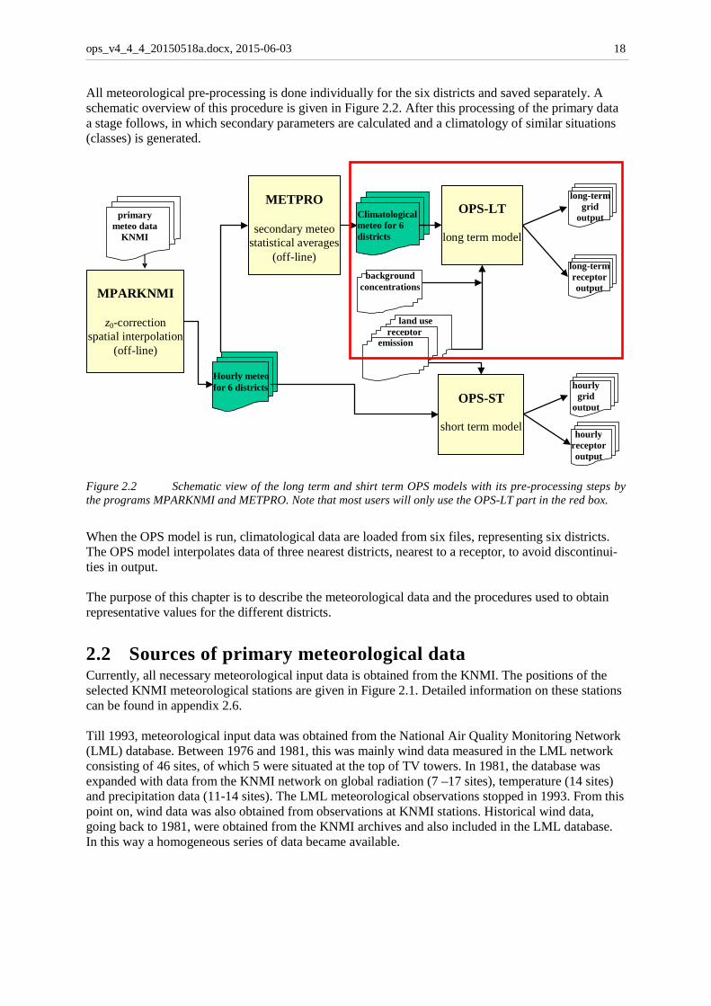
All meteorological pre-processing is done individually for the six districts and saved separately. A schematic overview of this procedure is given in Figure 2.2. After this processing of the primary data a stage follows, in which secondary parameters are calculated and a climatology of similar situations (classes) is generated.

Figure 2.2 Schematic view of the long term and shirt term OPS models with its pre-processing steps by the programs MPARKNMI and METPRO. Note that most users will only use the OPS-LT part in the red box.

When the OPS model is run, climatological data are loaded from six files, representing six districts. The OPS model interpolates data of three nearest districts, nearest to a receptor, to avoid discontinui-ties in output. The purpose of this chapter is to describe the meteorological data and the procedures used to obtain representative values for the different districts.

2.2 Sources of primary meteorological data Currently, all necessary meteorological input data is obtained from the KNMI. The positions of the selected KNMI meteorological stations are given in Figure 2.1. Detailed information on these stations can be found in appendix 2.6. Till 1993, meteorological input data was obtained from the National Air Quality Monitoring Network (LML) database. Between 1976 and 1981, this was mainly wind data measured in the LML network consisting of 46 sites, of which 5 were situated at the top of TV towers. In 1981, the database was expanded with data from the KNMI network on global radiation (7 –17 sites), temperature (14 sites) and precipitation data (11-14 sites). The LML meteorological observations stopped in 1993. From this point on, wind data was also obtained from observations at KNMI stations. Historical wind data, going back to 1981, were obtained from the KNMI archives and also included in the LML database. In this way a homogeneous series of data became available.

OPS-LT

long term model

Hourly meteo for 6 districts

Climatological meteo for 6 districts

METPRO

secondary meteo

statistical averages (off-line)

OPS-ST

short term model

primary meteo data

KNMI

MPARKNMI

z0-correction

spatial interpolation (off-line)

long-term grid

output

long-term receptor output

hourly grid

output

hourly receptor output

land use receptor

emission

background concentrations

ops_v4_4_4_20150518a.docx, 2015-06-03

19

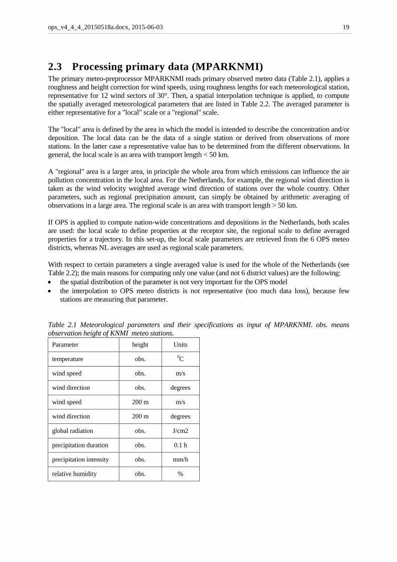
2.3 Processing primary data (MPARKNMI) The primary meteo-preprocessor MPARKNMI reads primary observed meteo data (Table 2.1), applies a roughness and height correction for wind speeds, using roughness lengths for each meteorological station, representative for 12 wind sectors of 30°. Then, a spatial interpolation technique is applied, to compute the spatially averaged meteorological parameters that are listed in Table 2.2. The averaged parameter is either representative for a "local" scale or a "regional" scale. The "local" area is defined by the area in which the model is intended to describe the concentration and/or deposition. The local data can be the data of a single station or derived from observations of more stations. In the latter case a representative value has to be determined from the different observations. In general, the local scale is an area with transport length < 50 km. A "regional" area is a larger area, in principle the whole area from which emissions can influence the air pollution concentration in the local area. For the Netherlands, for example, the regional wind direction is taken as the wind velocity weighted average wind direction of stations over the whole country. Other parameters, such as regional precipitation amount, can simply be obtained by arithmetic averaging of observations in a large area. The regional scale is an area with transport length > 50 km. If OPS is applied to compute nation-wide concentrations and depositions in the Netherlands, both scales are used: the local scale to define properties at the receptor site, the regional scale to define averaged properties for a trajectory. In this set-up, the local scale parameters are retrieved from the 6 OPS meteo districts, whereas NL averages are used as regional scale parameters. With respect to certain parameters a single averaged value is used for the whole of the Netherlands (see Table 2.2); the main reasons for computing only one value (and not 6 district values) are the following: • the spatial distribution of the parameter is not very important for the OPS model • the interpolation to OPS meteo districts is not representative (too much data loss), because few

stations are measuring that parameter. Table 2.1 Meteorological parameters and their specifications as input of MPARKNMI. obs. means observation height of KNMI meteo stations.

Parameter height Units

temperature obs. 0C

wind speed obs. m/s

wind direction obs. degrees

wind speed 200 m m/s

wind direction 200 m degrees

global radiation obs. J/cm2

precipitation duration obs. 0.1 h

precipitation intensity obs. mm/h

relative humidity obs. %

ops_v4_4_4_20150518a.docx, 2015-06-03

20

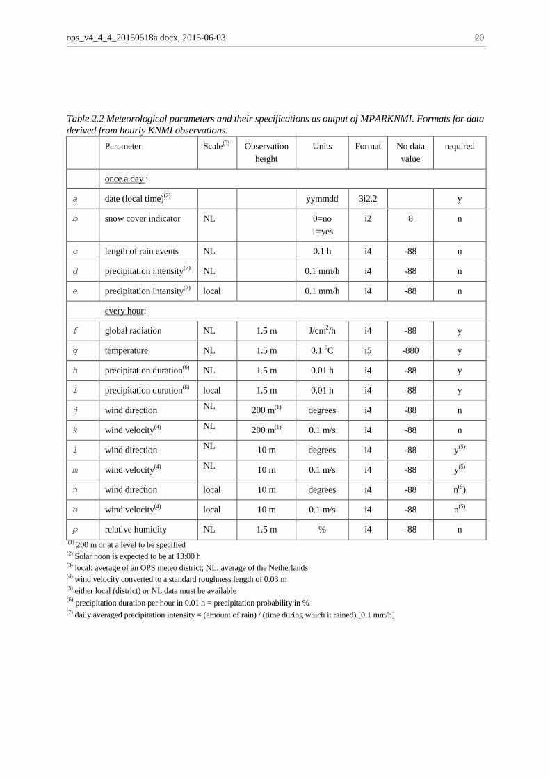
Table 2.2 Meteorological parameters and their specifications as output of MPARKNMI. Formats for data derived from hourly KNMI observations.

Parameter Scale(3) Observation height

Units Format No data value

required

once a day :

a date (local time)(2) yymmdd 3i2.2 y

b snow cover indicator NL 0=no 1=yes

i2 8 n

c length of rain events NL 0.1 h i4 -88 n

d precipitation intensity(7) NL 0.1 mm/h i4 -88 n

e precipitation intensity(7) local 0.1 mm/h i4 -88 n

every hour:

f global radiation NL 1.5 m J/cm2/h i4 -88 y

g temperature NL 1.5 m 0.1 0C i5 -880 y

h precipitation duration(6) NL 1.5 m 0.01 h i4 -88 y

i precipitation duration(6) local 1.5 m 0.01 h i4 -88 y

j wind direction NL 200 m(1) degrees i4 -88 n

k wind velocity(4) NL 200 m(1) 0.1 m/s i4 -88 n

l wind direction NL 10 m degrees i4 -88 y(5)

m wind velocity(4) NL 10 m 0.1 m/s i4 -88 y(5)

n wind direction local 10 m degrees i4 -88 n(5)

o wind velocity(4) local 10 m 0.1 m/s i4 -88 n(5)

p relative humidity NL 1.5 m % i4 -88 n (1) 200 m or at a level to be specified (2) Solar noon is expected to be at 13:00 h (3) local: average of an OPS meteo district; NL: average of the Netherlands (4) wind velocity converted to a standard roughness length of 0.03 m (5) either local (district) or NL data must be available (6) precipitation duration per hour in 0.01 h = precipitation probability in % (7) daily averaged precipitation intensity = (amount of rain) / (time during which it rained) [0.1 mm/h]

ops_v4_4_4_20150518a.docx, 2015-06-03

21

An overview of MPARKNMI is shown in Figure 2.3.

Figure 2.3 Processing of primary meteorological data by MPARKNMI.

2.3.1 Calculating the potential wind speed The OPS model uses spatially averaged meteorological data rather than point data. Before any form of spatial averaging can take place, it is necessary that all wind data is converted to standard conditions. Not all stations have the same measuring height. Moreover, the terrain conditions are not the same for all the stations. Therefore, wind velocities are converted to a potential wind speed, defined as the wind at 10 m height and at a roughness length of 0.03 m, according to the method described in section 0. Because the roughness length is not the same in all wind directions, conversion is applied as a function of wind direction.

2.3.2 Spatial averaging of meteorological data The spatial averaging method chosen here is first interpolating the data over the Netherlands, using all the available stations (see Figure 2.1 and Table 2.6) and then calculating district averages. In this way, the data are optimally used and the information of nearby stations is used automatically, if local stations fail. In earlier approaches, a number of stations were selected to be representative for an OPS meteo district. The major drawback of such a method is that, if data sets change, one has to make new selections with the risk of changing trends in the district. Also, the chance that for a given hour none of the selected stations will provide valid information is high, resulting in a high percentage of missing data. Parameters are interpolated using a 10 x 10 km grid over the Netherlands. Given a set of N observations, the resulting parameter value for a grid cell (k,l) of the grid is:

roughness and height correction for each station

spatial interpolation

spatial averaging over 6 districts

)

hourly data for 6 districts

MPARKNMI

hourly observations KNMI

10 m wind speed 10 m wind direction 200 m wind speed 200 m wind direction

hourly observations KNMI

temperature relative humidity global radiation precipitation amount precipitation duration snow cover

roughness data for each station (12 wind directions)

district mask

ops_v4_4_4_20150518a.docx, 2015-06-03

22

∑

∑

=

== N

i

N

ikl

iw

ixiwx

1

1

)(

)()(, (2.1)

with x(i): parameter value at station i and w(i): weighing factor for station i, depending on the distance r between the grid point and the position of the measuring station according to:

−=

reprriw exp)( , (2.2)

Here, rrep is an interpolation distance which, considering the mean distance between the stations, is fixed at 10 km.

0 5 10 15 20 25 30 35 40 45 500

0.2

0.4

0.6

0.8

1

r [km]

wei

ghin

g fa

ctor

Figure 2.4 Weighing factor as function of distance r.

If the contribution of each station to each grid point has been calculated, then the parameters are spatially averaged to district averages by using a mask according to Figure 2.1. 2.3.2.1 Wind direction The potential wind speed u in combination with the wind direction is split into an ux and uy vector and district averages are computed as above for ux and uy. The resulting wind direction per district is simply calculated by taking the arctangent of the vectors. If the observations indicate a variable wind direction, the observation is ignored. In such a case, the remaining stations determine the direction of the wind in the district. 2.3.2.2 Wind speed Spatial averaging of wind speed is done using the same interpolation procedure. Considering the use of wind speed in the model (mainly to derive turbulence parameters), the interpolation is independent of wind direction. The minimum wind speed of individual observations is set at 0.5 m/s. This takes the trigger threshold of the anemometers used into account (in the order of 0.4 m/s) to some extent, and also the fact that wind speed is given in 1 m/s units (before July 1996, wind speeds were specified in knots ≈ 0.5 m/s). Ignoring situations with zero wind speed would introduce a bias in the ‘average’ wind speed, and therefore will lead to larger errors in modelling than using lower limit values. 2.3.2.3 Other parameters Interpolation of global radiation, temperature, relative humidity, precipitation duration and precipitation intensity is carried out in the same way as for wind speed. The length of rain events and snow cover are not spatially interpolated, but apply always for the Netherlands as a whole.

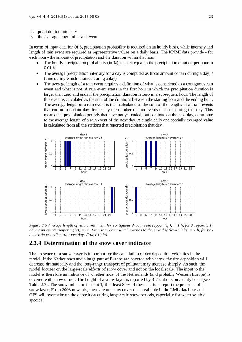
2.3.3 Calculation of precipitation characteristics Precipitation events in the OPS model are described with three parameters: 1. precipitation probability

ops_v4_4_4_20150518a.docx, 2015-06-03

23

2. precipitation intensity 3. the average length of a rain event.

In terms of input data for OPS, precipitation probability is required on an hourly basis, while intensity and length of rain event are required as representative values on a daily basis. The KNMI data provide - for each hour - the amount of precipitation and the duration within that hour.

• The hourly precipitation probability (in %) is taken equal to the precipitation duration per hour in 0.01 h.

• The average precipitation intensity for a day is computed as (total amount of rain during a day) / (time during which it rained during a day).

• The average length of a rain event requires a definition of what is considered as a contiguous rain event and what is not. A rain event starts in the first hour in which the precipitation duration is larger than zero and ends if the precipitation duration is zero in a subsequent hour. The length of this event is calculated as the sum of the durations between the starting hour and the ending hour. The average length of a rain event is then calculated as the sum of the lengths of all rain events that end on a certain day divided by the number of rain events that end during that day. This means that precipitation periods that have not yet ended, but continue on the next day, contribute to the average length of a rain event of the next day. A single daily and spatially averaged value is calculated from all the stations that reported precipitation that day.

1 3 5 7 9 11 13 15 17 19 21 230

0.5

1

hour

prec

ipita

tion

dura

tion

(h)

day 3average length rain event = 1 h

1 3 5 7 9 11 13 15 17 19 21 230

0.5

1

hour

prec

ipita

tion

dura

tion

(h)

day 2average length rain event = 3 h

1 3 5 7 9 11 13 15 17 19 21 230

0.5

1

hour

prec

ipita

tion

dura

tion

(h)

day 7average length rain event = 2 h

1 3 5 7 9 11 13 15 17 19 21 230

0.5

1

hour

prec

ipita

tion

dura

tion

(h)

day 6average length rain event = 0 h

Figure 2.5 Average length of rain event = 3h, for contiguous 3-hour rain (upper left); = 1 h, for 3 separate 1-hour rain events (upper right); = 0h, for a rain event which extends to the next day (lower left); = 2 h, for two hour rain extending over two days (lower right).

2.3.4 Determination of the snow cover indicator The presence of a snow cover is important for the calculation of dry deposition velocities in the model. If the Netherlands and a large part of Europe are covered with snow, the dry deposition will decrease dramatically and the long-range transport of pollutant may increase sharply. As such, the model focuses on the large-scale effects of snow cover and not on the local scale. The input to the model is therefore an indicator of whether most of the Netherlands (and probably Western Europe) is covered with snow or not. The height of a snow layer is reported by 3-7 stations on a daily basis (see Table 2.7). The snow indicator is set at 1, if at least 80% of these stations report the presence of a snow layer. From 2003 onwards, there are no snow cover data available in the LML database and OPS will overestimate the deposition during large scale snow periods, especially for water soluble species.

ops_v4_4_4_20150518a.docx, 2015-06-03

24

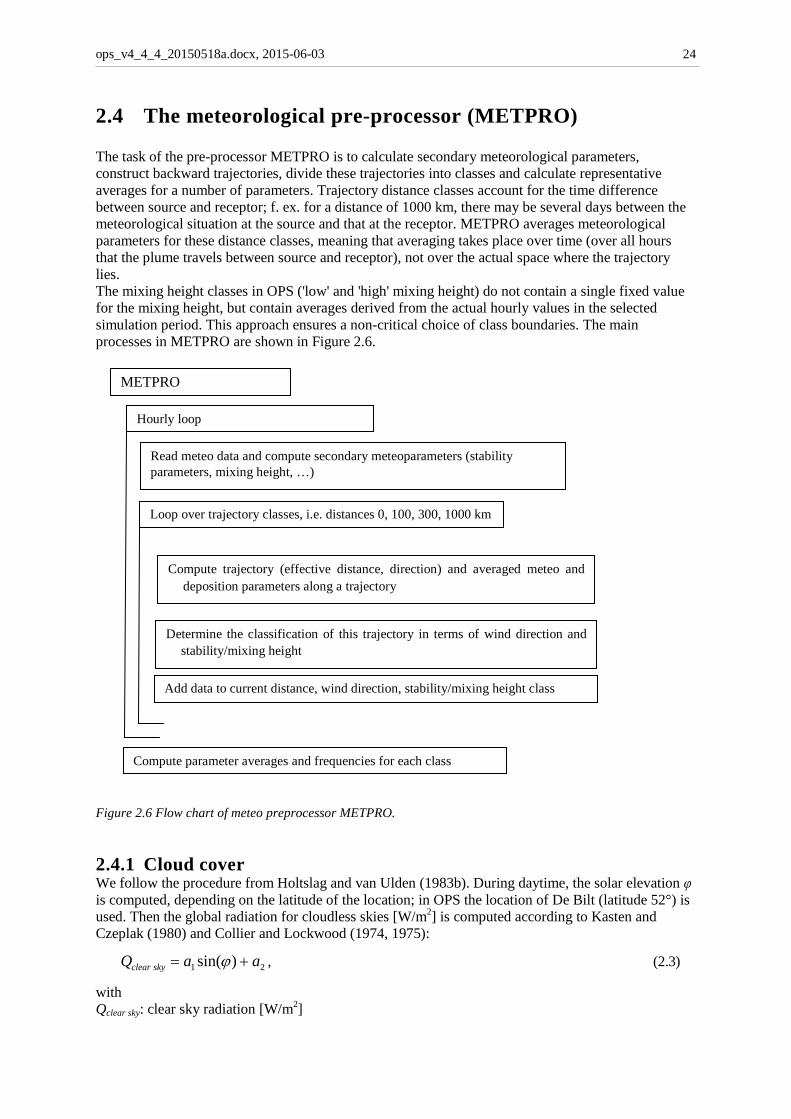
2.4 The meteorological pre-processor (METPRO) The task of the pre-processor METPRO is to calculate secondary meteorological parameters, construct backward trajectories, divide these trajectories into classes and calculate representative averages for a number of parameters. Trajectory distance classes account for the time difference between source and receptor; f. ex. for a distance of 1000 km, there may be several days between the meteorological situation at the source and that at the receptor. METPRO averages meteorological parameters for these distance classes, meaning that averaging takes place over time (over all hours that the plume travels between source and receptor), not over the actual space where the trajectory lies. The mixing height classes in OPS ('low' and 'high' mixing height) do not contain a single fixed value for the mixing height, but contain averages derived from the actual hourly values in the selected simulation period. This approach ensures a non-critical choice of class boundaries. The main processes in METPRO are shown in Figure 2.6.

Figure 2.6 Flow chart of meteo preprocessor METPRO.

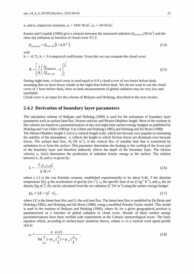
2.4.1 Cloud cover We follow the procedure from Holtslag and van Ulden (1983b). During daytime, the solar elevation φ is computed, depending on the latitude of the location; in OPS the location of De Bilt (latitude 52°) is used. Then the global radiation for cloudless skies [W/m2] is computed according to Kasten and Czeplak (1980) and Collier and Lockwood (1974, 1975):

21 )sin( aaQ skyclear += ϕ , (2.3)

with Qclear sky: clear sky radiation [W/m2]

Read meteo data and compute secondary meteoparameters (stability parameters, mixing height, …)

Compute trajectory (effective distance, direction) and averaged meteo and deposition parameters along a trajectory

Determine the classification of this trajectory in terms of wind direction and stability/mixing height

Loop over trajectory classes, i.e. distances 0, 100, 300, 1000 km

Hourly loop

Compute parameter averages and frequencies for each class

METPRO

Add data to current distance, wind direction, stability/mixing height class

ops_v4_4_4_20150518a.docx, 2015-06-03

25

a1 and a2 empirical constants, a1 = 1041 W/m2, a2 = -69 W/m2. Kasten and Czeplak (1980) give a relation between the measured radiation Qmeasured [W/m2] and the clear sky radiation as function of cloud cover N [-]:

( )211 b

skyclearmeasured NbQ = Q + , (2.4)

with b1 = -0.75, b2 = 3.4 empirical coefficients. From this we can compute the cloud cover:

2

1

1

11 b

skyclear

measured

QQ

bN

−= . (2.5)

During night time, a cloud cover is used equal to 0.9 x cloud cover of two hours before dusk, assuming that we have fewer clouds in the night than before dusk. We do not want to use the cloud cover of 1 hour before dusk, since at dusk measurements of global radiation may be very low and unreliable. Cloud cover is an input for the scheme of Beljaars and Holtslag, described in the next section.

2.4.2 Derivation of boundary layer parameters The calculation scheme of Beljaars and Holtslag (1990) is used for the estimation of boundary layer parameters such as surface heat flux, friction velocity and Monin-Obukhov length. Most of the routines in this scheme are based on a parameterization of day and night-time surface energy budgets as published by Holtslag and Van Ulden (1983a); Van Ulden and Holtslag (1985) and Holtslag and De Bruin (1988). The Monin-Obukhov length L [m] is a vertical length scale, which has become very popular in estimating the stability of the atmosphere. -L reflects the height to which friction forces are dominant over buoyant forces. The surface heat flux, H0 [W m-2], is the vertical flux of sensible heat that is transferred by turbulence to or from the surface. This parameter determines the heating or the cooling of the lower part of the boundary layer and therefore indirectly affects the depth of the boundary layer. The friction velocity u* [m/s] determines the production of turbulent kinetic energy at the surface. The relation between L, H0 and u* is given by:

κ

ρ H g

u c T = L

0

*pa3

− , (2.6)

where κ [-] is the von Kármán constant, established experimentally to be about 0.40, T the absolute temperature [K], g the acceleration of gravity [m s-2], cp the specific heat of air [J kg-1 K-1], and ρa the air density [kg m-3]. H0 can be calculated from the net radiation Q* [W m-2] using the surface energy budget:

s*

0 G- Q = LE + H , (2.7)

where LE is the latent heat flux and Gs the soil heat flux. The latent heat flux is modelled by De Bruin and Holtslag (1982), and Holtslag and De Bruin (1988), using a modified Priestly-Taylor model. This model is used in the routines of Beljaars and Holtslag (1990), where H0 for a given geographical position is parameterized as a function of global radiation or cloud cover. Results of these surface energy parameterizations have been verified with experiments at the Cabauw meteorological tower. The basic equation which, according to surface-layer similarity theory, relates u* to a vertical wind speed profile u(z) is:

Lz +

Lz -

zz

zu = umm

*

)()()(ln

)(0

0ψψ

κ, (2.8)

ops_v4_4_4_20150518a.docx, 2015-06-03

26

where z is an arbitrary height in the surface layer, z0 the surface layer roughness length of the terrain (for a classification, see Wieringa (1981)). The functions ψm, are stability correction functions for momentum, which read as follows (Paulson 1970, Holtslag 1984): for z/L < 0:

) 61 - 1 ( = with

2π)(arctan2)

21(ln)

21(ln2)(

4/1

2

Lzx

+ x - x+ + x + = Lz mψ

(2.9)

for z/L > 200:

72.100.7- )( −Lz =

Lz mψ (2.10)

for 0 ≤ z/L ≤ 200:

72.10)35.0exp()72.1075.0(0.7- )( −⋅−−Lz

Lz

Lz =

Lz mψ . (2.11)

Equations (2.6)-(2.11) are iteratively solved to obtain u* and L (Beljaars and Holtslag, 1990). The following minimal values are imposed: |L| = 5 m, u* = 0.04 m/s. From Eq. (2.8) relations can be derived for wind speed profile calculations or for the translation of wind speed observations to situations with different z0. In section 2.4.5 more details on the wind speed profile and stability correction functions are given.

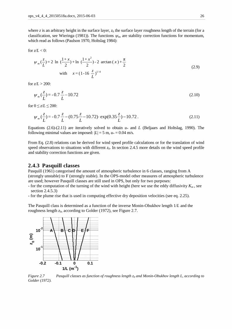
2.4.3 Pasquill classes Pasquill (1961) categorised the amount of atmospheric turbulence in 6 classes, ranging from A (strongly unstable) to F (strongly stable). In the OPS-model other measures of atmospheric turbulence are used; however Pasquill classes are still used in OPS, but only for two purposes: - for the computation of the turning of the wind with height (here we use the eddy diffusivity Km , see

section 2.4.5.3) - for the plume rise that is used in computing effective dry deposition velocities (see eq. 2.25). The Pasquill class is determined as a function of the inverse Monin-Obukhov length 1/L and the roughness length z0, according to Golder (1972), see Figure 2.7.

-0.2 -0.1 0 0.1

10-2

10-1

A B C D E F

1/L (m-1)

z 0 (m)

Figure 2.7 Pasquill classes as function of roughness length z0 and Monin-Obukhov length L, according to Golder (1972).

ops_v4_4_4_20150518a.docx, 2015-06-03

27

Table 2.3 Pasquill classes and corresponding Monin-Obukhov length L [m] and eddy diffusivity of the boundary layer Km [m2/s]

Pasquill class characterisation range of L for z0 = 0.1 m Km [m2/s] A strongly unstable [-10, 0] 50 B unstable [-28, -10] 40 C weakly unstable [-147, -28] 30 D neutral [-∞, -147], [135, ∞] 10 E stable [27, 135] 3 F strongly stable [0, 27] 1 The following adaptations have been implemented in order to remain more closely to the classification of the Dutch National model (TNO, 1976): Q* ≤ 0 W/m2, A-D D Q* > 0 W/m2, E-F D N > 8

6 D E-F, v > 3 m/s, N > 8

3 D Q* ≤ 0 W/m2, 2 m/s < v ≤ 3 m/s, 8

3 < N < 86 E.

2.4.4 Estimation of mixing heights Although it was possible, in principle, to use temperature profiles from radio soundings for the determination of the mixing layer height, estimation of the mixing height on the basis of surface-layer parameters was preferred. The main reason for this is that the inversion height is usually taken at the height of the dominant temperature jump in the profile, so is valid for ‘aged’ pollutants, while this model needs the height of the first layer starting at the surface that effectively isolates the surface layer from higher parts of the boundary layer. Moreover, temperature profiles from radio soundings have a limited resolution in the lower boundary layer (Driedonks, 1981). 2.4.4.1 Stable and neutral conditions Strictly speaking, the nocturnal boundary-layer height is not stationary (Nieuwstadt, 1981). Proposed prognostic models usually take the form of a relaxation process, in which the actual boundary-layer height approaches a diagnostically determined equilibrium value. It turns out that the time scale of the relaxation process is very large and therefore the equilibrium value can be used as an estimator for the actual boundary-layer depth (Nieuwstadt, 1984). For this reason the direct applicability of diagnostic relationships was evaluated. A simple diagnostic relation of the form:

fu c = z

c

*i 1 , (2.12)

as first proposed by Delage (1974), was found to give satisfactory results for both stable and neutral atmospheric conditions. In this equation fc is the Coriolis parameter and c1 a proportionality coefficient. From the data set of night-time acoustic sounder observations at Cabauw (Nieuwstadt, 1981), c1 was estimated at 0.08. Equation (2.12) was also tested using acoustic sounder observations carried out at Bilthoven in 1981 during daytime. Values for c1 found were 0.086 during neutral atmospheric conditions and 0.092 for neutral + stable cases. For the present model Eq. (2.12) is adopted, with c1 = 0.092 for both neutral and stable cases.

ops_v4_4_4_20150518a.docx, 2015-06-03

28

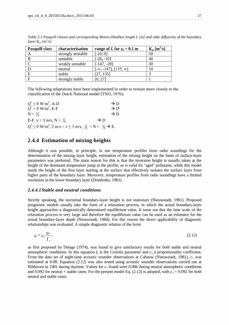
2.4.4.2 Unstable conditions Adequate diagnostic equations do not exist for the depth of the unstable atmospheric boundary layer (Van Ulden and Holtslag, 1985). It is common practice to use rate equations (Tennekes, 1973; Stull, 1983) for describing the rise of an inversion by buoyancy as well as by mechanical forces. The model adopted here is based on the model of Tennekes (1973) and describes the growth of the convective boundary layer for a rather idealized situation. More details on this approach are given in Van Jaarsveld (1995). In Figure 2.8, model results and observations are compared as a function of time of the day for the ten-day data set of Driedonks (1981). Indeed, no systematic difference is observed in the average course of the mixed-layer height in the morning. Considering the way mixed-layer heights are used in the OPS model, namely, as averages for typical situations, one can conclude the current approach to lead to the desired results.

0

200

400

600

800

5 6 7 8 9 10 11 12 13

time (UTC)

z i (m

) observed

modelled

Figure 2.8 Comparison of modelled and observed mixing-layer heights (average of ten

convective days) at Cabauw.

2.4.5 The wind profile Pollutants are emitted at various heights in the atmosphere. Moreover, due to turbulent mixing, the effective transport height of a pollutant may change in time. Wind speed data are usually available for one or two discrete observation levels. What is needed for the description of dispersion and transport of pollutants is a relation between wind speeds at different heights. It is common practice to base this relation for the lower boundary layer on Monin-Obukhov similarity theory. The following general expression for the wind speed at height z can be derived from Eq. (2.8):

+

+

Lz

Lz -

zz

Lz

Lz -

zz

zu = zu

mm

mm

)()()(ln

)()()(ln)()(

01

0

1

0

01

ψψ

ψψ, (2.13)

where z1 is the height at which a wind observation is available. The functions ψm given by Eq. (2.9) - (2.11) are, strictly speaking, only valid for the surface layer (z0 << z < |L|). However, several authors have derived correction functions describing the wind speed relation up to the top of the mixing layer (Carson and Richards, 1978; Garratt et al., 1982; Holtslag, 1984; Van Ulden and Holtslag, 1985). A function which in combination with Eq. (2.13) fits the wind speed observations at the Cabauw tower in stable situations up to 200 m well, is (Holtslag, 1984):

ops_v4_4_4_20150518a.docx, 2015-06-03

29

,) 51 - 1 ( = with

0,2π)(arctan2)

21(ln)

21(ln2)(

4/1

2

Lzx

L+ x - x+ + x + = Lz m ≤ψ

(2.14)

] )0.29(exp1 [17)( Lz - - - =

Lz mψ , L > 0. (2.15)

This function is used in the model instead of Eq. (2.9) – (2.11) in computing the wind profile, where it should be noted that for L ≤ 0, the terms ψm(z0/L), present in Eq. (2.8), have been dropped because they are comparatively small.

0 5 10 15 20 25 30 350

10

20

30

40

50

u (m/s)

heig

ht (m

)

U1U2N1N2S1S2

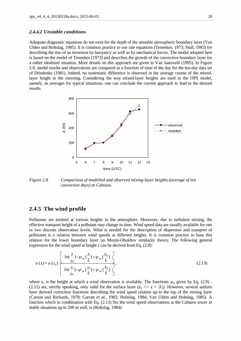
Figure 2.9 Vertical wind profile computed with eq. 2.8 for the stability/mixing height classes used

in OPS. Values of u*, L are from Table 2.5,z0 = 0.03 m. . 2.4.5.1 Combining wind observations An expression similar to Eq. (2.13) can be derived from (2.8) to translate u(z;z0) measured at measuring height z at a location with roughness z0 to a potential wind speed u(z1;z0'') at a reference level z1 (= 10 m) representative for a reference z0" = 0.03 m. The procedure is to convert u(z;z0) to u(z2;z0) (z2 taken 60 m) and then to convert u(z2;z0'') = u(z2;z0) to u(z1;z0''). The assumption in this is that the wind speed at height z2 is not influenced by the local surface roughness.

0 0.2 0.4 0.6 0.8 1 1.2 1.4 1.60

1

2

3

4

5

6

7

8

local roughness (m)

win

d sp

eed

(m/s

)

uncorrectedcorrected, z0(site) = 0.1 mcorrected, z0(site) = 0.8 mcorrected, z0(site) = 1.5 m

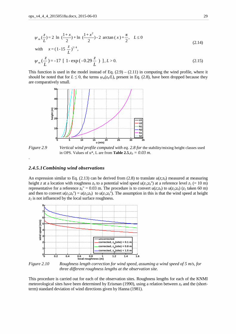
Figure 2.10 Roughness length correction for wind speed, assuming a wind speed of 5 m/s, for

three different roughness lengths at the observation site. This procedure is carried out for each of the observation sites. Roughness lengths for each of the KNMI meteorological sites have been determined by Erisman (1990), using a relation between z0 and the (short-term) standard deviation of wind directions given by Hanna (1981).

ops_v4_4_4_20150518a.docx, 2015-06-03

30

A representative wind speed for a district is calculated in the pre-processor by first normalizing the wind speeds at the different observational sites on the basis of an area-representative roughness length, and then averaging the roughness corrected wind speeds. A representative wind direction follows from the combined x and y components of the roughness-corrected wind vectors. 2.4.5.2 Observed wind speed profiles Although the logarithmic profile appears to fit observations well, it is used in the present model mainly for extrapolation to levels lower than the observation height (10 m). For the description of (horizontally averaged) transport velocities at different heights (up to 300 m) a relation of the form:

zz zu = (z)u 1

p

1)( , (2.16)

known as the power law, is used. The major advantage of this relation is that it can be easily fitted to observations. In the present case, p is derived hourly from the 10 m and 200 m observations at the Cabauw meteorological tower. The resulting p values range from 0.13 under unstable conditions (L > -30 m) to 0.45 under very stable conditions (L < 35 m). 2.4.5.3 Turning of the wind with height The direction of the wind as a function of height is important for the description of pollutant transport especially if this is done on the basis of surface-based observations. The turning of the wind in the 20 - 200 m layer was studied by Holtslag (1984) and Van Ulden and Holtslag (1985) on the basis of observations at the Cabauw tower. The latter authors give an empirical relation for A(z), the turning angle at height z relative to the surface wind direction, up to 200 m:

−

zzc - z A c= zAref

ref 76 exp1)()( , (2.17)

where A(zref ) is the turning angle at reference height zref ; c7 = 1.0 is an empirical coefficient, c6 is chosen such that for z = zref, A(z) = A(zref) or c6 = 1/(1-exp(-c7)) = 1.58. METPRO provides values of A(zref), based on measurements at the Cabauw tower in the period 1990 – 1996. Typical values of A(zref ) at zref = 200 m are 35, 12 and 9 degrees for stable, neutral and unstable situations, respectively. In METPRO, a trajectory is characterized by a single direction representative for mass flow of the pollutant. This direction is taken at a height equal to half of the maximum mixing height (100-2000 m) of the trajectory. The turning angle above the 150 – 300 m layer is not known from actual observations. On the assumption that the winds become geostrophic at some level above the observation height, an analy-tical description of the spiral given by Businger (1982) is used:

[ ] za z-a - G = U EEg )(cos)(exp1 (2.18)

[ ]m

cEEEg K

fa za z -a G = V 2=with ,)(sin)(exp , (2.19)

where Km is the (bulk) eddy diffusivity of the boundary layer and Ug and Vg the respective velocity vectors in the x and y directions, with the x-axis aligned with the geostrophic wind G. From Eqs. (2.18) and (2.19) the following expression has been derived for the turning angle AE(z) of the wind at height z relative to the geostrophic wind direction:

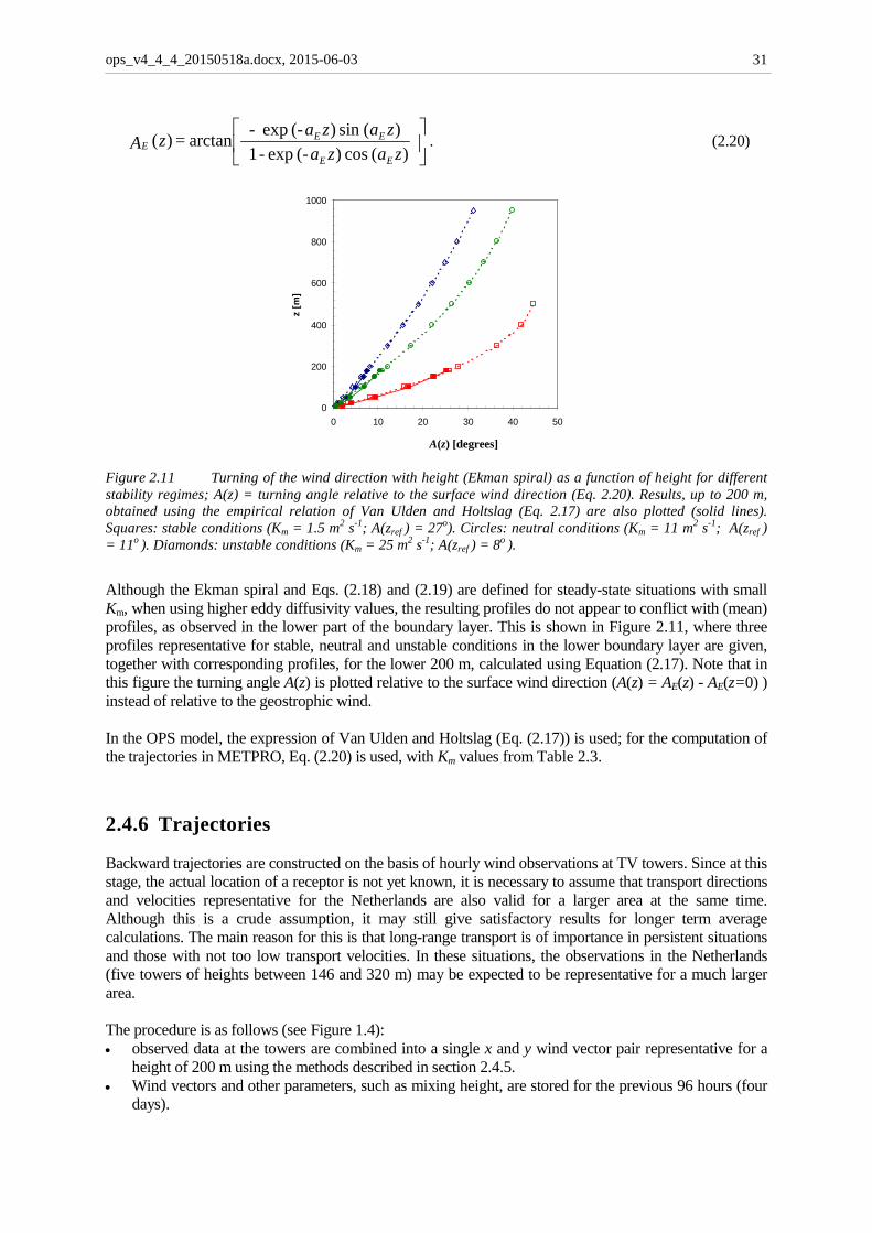
ops_v4_4_4_20150518a.docx, 2015-06-03

31

za za- - za za- - = z AEE

EEE )(cos)(exp1

)(sin)(exparctan)( . (2.20)

0

200

400

600

800

1000

0 10 20 30 40 50

AE(z) [o]

z [m

]

Figure 2.11 Turning of the wind direction with height (Ekman spiral) as a function of height for different stability regimes; A(z) = turning angle relative to the surface wind direction (Eq. 2.20). Results, up to 200 m, obtained using the empirical relation of Van Ulden and Holtslag (Eq. 2.17) are also plotted (solid lines). Squares: stable conditions (Km = 1.5 m2 s-1; A(zref ) = 27o). Circles: neutral conditions (Km = 11 m2 s-1; A(zref ) = 11o ). Diamonds: unstable conditions (Km = 25 m2 s-1; A(zref ) = 8o ).

Although the Ekman spiral and Eqs. (2.18) and (2.19) are defined for steady-state situations with small Km, when using higher eddy diffusivity values, the resulting profiles do not appear to conflict with (mean) profiles, as observed in the lower part of the boundary layer. This is shown in Figure 2.11, where three profiles representative for stable, neutral and unstable conditions in the lower boundary layer are given, together with corresponding profiles, for the lower 200 m, calculated using Equation (2.17). Note that in this figure the turning angle A(z) is plotted relative to the surface wind direction (A(z) = AE(z) - AE(z=0) ) instead of relative to the geostrophic wind. In the OPS model, the expression of Van Ulden and Holtslag (Eq. (2.17)) is used; for the computation of the trajectories in METPRO, Eq. (2.20) is used, with Km values from Table 2.3.

2.4.6 Trajectories Backward trajectories are constructed on the basis of hourly wind observations at TV towers. Since at this stage, the actual location of a receptor is not yet known, it is necessary to assume that transport directions and velocities representative for the Netherlands are also valid for a larger area at the same time. Although this is a crude assumption, it may still give satisfactory results for longer term average calculations. The main reason for this is that long-range transport is of importance in persistent situations and those with not too low transport velocities. In these situations, the observations in the Netherlands (five towers of heights between 146 and 320 m) may be expected to be representative for a much larger area. The procedure is as follows (see Figure 1.4): • observed data at the towers are combined into a single x and y wind vector pair representative for a

height of 200 m using the methods described in section 2.4.5. • Wind vectors and other parameters, such as mixing height, are stored for the previous 96 hours (four

days).

A(z) [degrees]

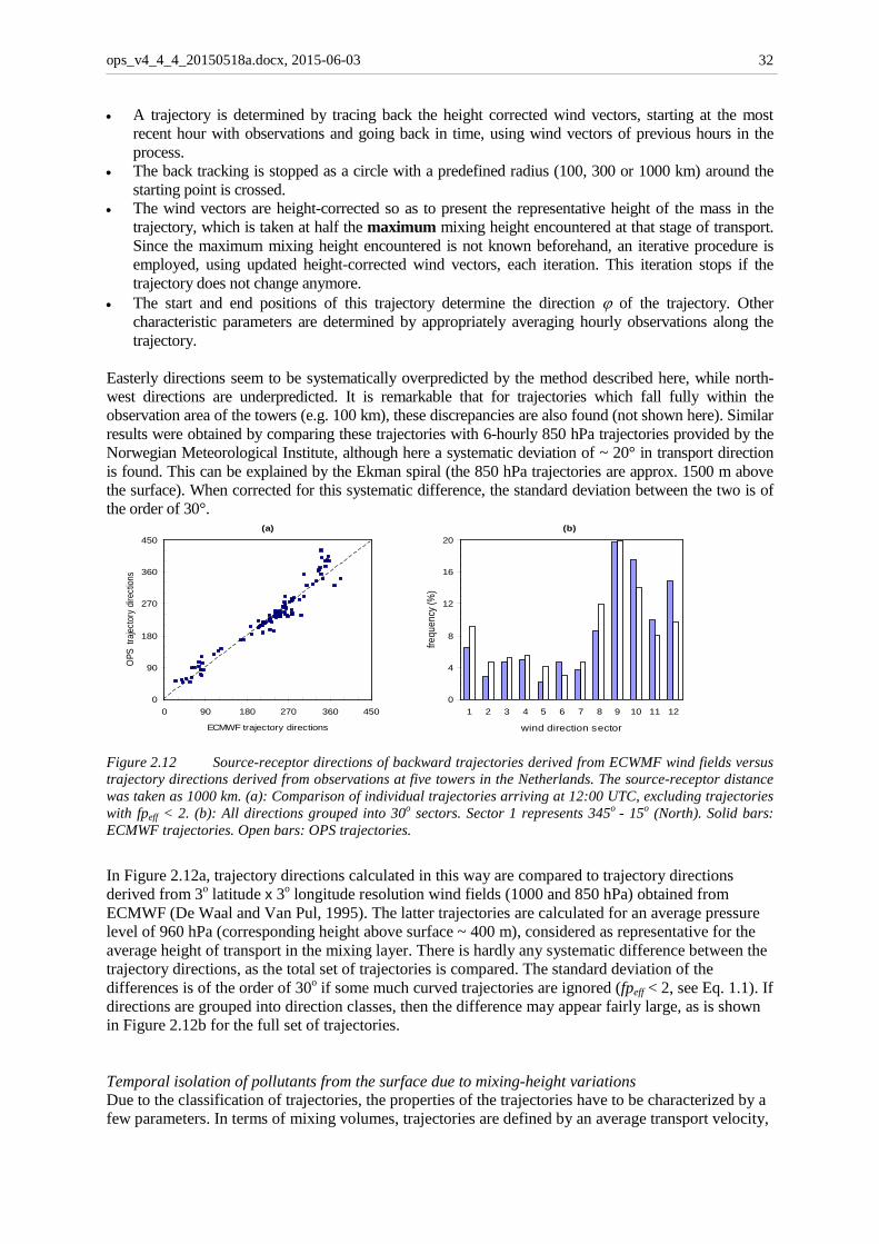
ops_v4_4_4_20150518a.docx, 2015-06-03

32

• A trajectory is determined by tracing back the height corrected wind vectors, starting at the most recent hour with observations and going back in time, using wind vectors of previous hours in the process.

• The back tracking is stopped as a circle with a predefined radius (100, 300 or 1000 km) around the starting point is crossed.

• The wind vectors are height-corrected so as to present the representative height of the mass in the trajectory, which is taken at half the maximum mixing height encountered at that stage of transport. Since the maximum mixing height encountered is not known beforehand, an iterative procedure is employed, using updated height-corrected wind vectors, each iteration. This iteration stops if the trajectory does not change anymore.

• The start and end positions of this trajectory determine the direction ϕ of the trajectory. Other characteristic parameters are determined by appropriately averaging hourly observations along the trajectory.

Easterly directions seem to be systematically overpredicted by the method described here, while north-west directions are underpredicted. It is remarkable that for trajectories which fall fully within the observation area of the towers (e.g. 100 km), these discrepancies are also found (not shown here). Similar results were obtained by comparing these trajectories with 6-hourly 850 hPa trajectories provided by the Norwegian Meteorological Institute, although here a systematic deviation of ~ 20° in transport direction is found. This can be explained by the Ekman spiral (the 850 hPa trajectories are approx. 1500 m above the surface). When corrected for this systematic difference, the standard deviation between the two is of the order of 30°.

0

90

180

270

360

450

0 90 180 270 360 450

ECMWF trajectory directions

OPS

tra

jecto

ry d

irect

ions

(a)

0

4

8

12

16

20

1 2 3 4 5 6 7 8 9 10 11 12

wind direction sector

frequ

ency

(%)

(b)

Figure 2.12 Source-receptor directions of backward trajectories derived from ECWMF wind fields versus trajectory directions derived from observations at five towers in the Netherlands. The source-receptor distance was taken as 1000 km. (a): Comparison of individual trajectories arriving at 12:00 UTC, excluding trajectories with fpeff < 2. (b): All directions grouped into 30o sectors. Sector 1 represents 345o - 15o (North). Solid bars: ECMWF trajectories. Open bars: OPS trajectories.

In Figure 2.12a, trajectory directions calculated in this way are compared to trajectory directions derived from 3o latitude x 3o longitude resolution wind fields (1000 and 850 hPa) obtained from ECMWF (De Waal and Van Pul, 1995). The latter trajectories are calculated for an average pressure level of 960 hPa (corresponding height above surface ~ 400 m), considered as representative for the average height of transport in the mixing layer. There is hardly any systematic difference between the trajectory directions, as the total set of trajectories is compared. The standard deviation of the differences is of the order of 30o if some much curved trajectories are ignored (fpeff < 2, see Eq. 1.1). If directions are grouped into direction classes, then the difference may appear fairly large, as is shown in Figure 2.12b for the full set of trajectories. Temporal isolation of pollutants from the surface due to mixing-height variations Due to the classification of trajectories, the properties of the trajectories have to be characterized by a few parameters. In terms of mixing volumes, trajectories are defined by an average transport velocity,

ops_v4_4_4_20150518a.docx, 2015-06-03

33

u tra, and the maximum mixing height, zi max, which has appeared during transport. In reality the mixing height that an air parcel encounters on its way to the receptor point can be lower than this height. Moreover, the parcel may be transported above the mixing layer part of the time. In such a situation the pollution in the parcel is not removed by dry deposition, a process which only occurs at the surface. Standard averaging of dry deposition velocities over a trajectory, gives us an average dry deposition velocity

)(11

t vNv d

N

=ttrad ∑= , (2.21)

where N is the number of (hourly) intervals and vd(t) the dry deposition velocity at time t. To account for the effects described above, ‘effective’ dry deposition velocities ( tradv ~ ) are introduced, which account for the total loss of material on its way from source to receptor and are related to zi max. The procedure is to follow the air parcel and to integrate the loss of material due to dry deposition, taking into account transport of pollutant mass due to a changing mixing height and keeping track of the mass which is isolated from the surface and does not take part in the deposition process. Mass loss due to deposition is described by the following differential equation:

)()()()()(

d)(d

tztMtvtCtvF

ttM

iddd −=−== , (2.22)

with M(t): total cross-wind integrated pollutant mass in the mixing layer [g/m2], Fd :deposition flux [g/m2/s], C(t): concentration [g/m3] and zi(t) the actual mixing height at time t [m]. Integrating over a time step [t, t+Δt], this differential equation has as solution

∆−=∆+

)(exp)()(

tztvtMttM

i

d . (2.23)

Using Eq. 2.23 for successive time steps, the mass at t = tend , the total travel time of the trajectory, can be computed. Now the effective dry deposition velocity tradv ~ for the trajectory can be derived from:

−=⇔

−=

)0()(ln~

~exp)0()(

MtM

tz

vz

tvMtM end

end

maxitrad

maxi

endtradend , (2.24)

where zi max is the maximum mixing height over the trajectory. It is clear that the fraction of the time that pollutants spend above the mixing layer strongly depends on the source height. Therefore the calculation of effective dry deposition velocities is carried out in the pre-processor for two characteristic source heights: a high source (unit strength, 100 m stack height and plume rise according to Briggs (1975) for a heat content of 20 MW), and a low source (35 m, no plume rise). The latter is representative for sources which always emit within the mixing layer and the former for larger point sources which emit temporarily above the mixing layer. The effective dry deposition velocities calculated in this way are used in the model in the form of correction factors to the deposition velocity and as such are included in the meteorological data set:

vv = h x,f

trad

tradd

~)( , (2.25)

where x denotes the source receptor distance and h the source height. fd has a range of 0.70 - 1.7 with a mean value of 1.2 for the elevated source. For the low source this range is 0.80 - 2.2, with a mean value of 1.4 (sulphur dioxide, 1000 km trajectories). Formally, these correction factors are substance-specific. However, only small differences are found for the usual range of dry deposition velocities. From tests it appears that transport in or above the mixing layer at night explains most of the difference between

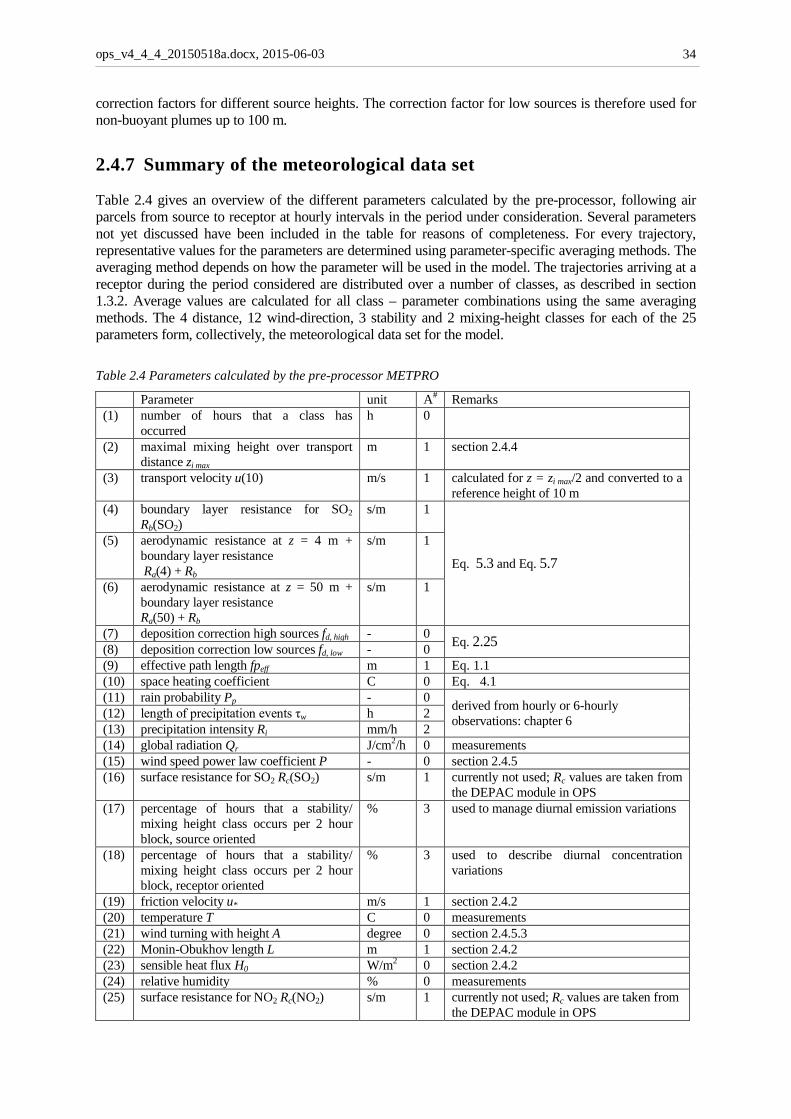
ops_v4_4_4_20150518a.docx, 2015-06-03

34

correction factors for different source heights. The correction factor for low sources is therefore used for non-buoyant plumes up to 100 m.

2.4.7 Summary of the meteorological data set Table 2.4 gives an overview of the different parameters calculated by the pre-processor, following air parcels from source to receptor at hourly intervals in the period under consideration. Several parameters not yet discussed have been included in the table for reasons of completeness. For every trajectory, representative values for the parameters are determined using parameter-specific averaging methods. The averaging method depends on how the parameter will be used in the model. The trajectories arriving at a receptor during the period considered are distributed over a number of classes, as described in section 1.3.2. Average values are calculated for all class – parameter combinations using the same averaging methods. The 4 distance, 12 wind-direction, 3 stability and 2 mixing-height classes for each of the 25 parameters form, collectively, the meteorological data set for the model. Table 2.4 Parameters calculated by the pre-processor METPRO

Parameter unit A# Remarks (1) number of hours that a class has

occurred h 0

(2) maximal mixing height over transport distance zi max

m 1 section 2.4.4

(3) transport velocity u(10) m/s 1 calculated for z = zi max/2 and converted to a reference height of 10 m

(4) boundary layer resistance for SO2 Rb(SO2)

s/m 1

Eq. 5.3 and Eq. 5.7

(5) aerodynamic resistance at z = 4 m + boundary layer resistance Ra(4) + Rb

s/m 1

(6) aerodynamic resistance at z = 50 m + boundary layer resistance Ra(50) + Rb

s/m 1

(7) deposition correction high sources fd, high - 0 Eq. 2.25 (8) deposition correction low sources fd, low - 0 (9) effective path length fpeff m 1 Eq. 1.1 (10) space heating coefficient C 0 Eq. 4.1 (11) rain probability Pp - 0 derived from hourly or 6-hourly

observations: chapter 6 (12) length of precipitation events τw h 2 (13) precipitation intensity Ri mm/h 2 (14) global radiation Qr J/cm2/h 0 measurements (15) wind speed power law coefficient P - 0 section 2.4.5 (16) surface resistance for SO2 Rc(SO2) s/m 1 currently not used; Rc values are taken from

the DEPAC module in OPS (17) percentage of hours that a stability/

mixing height class occurs per 2 hour block, source oriented

% 3 used to manage diurnal emission variations

(18) percentage of hours that a stability/ mixing height class occurs per 2 hour block, receptor oriented

% 3 used to describe diurnal concentration variations

(19) friction velocity u* m/s 1 section 2.4.2 (20) temperature T C 0 measurements (21) wind turning with height A degree 0 section 2.4.5.3 (22) Monin-Obukhov length L m 1 section 2.4.2 (23) sensible heat flux H0 W/m2 0 section 2.4.2 (24) relative humidity % 0 measurements (25) surface resistance for NO2 Rc(NO2) s/m 1 currently not used; Rc values are taken from

the DEPAC module in OPS

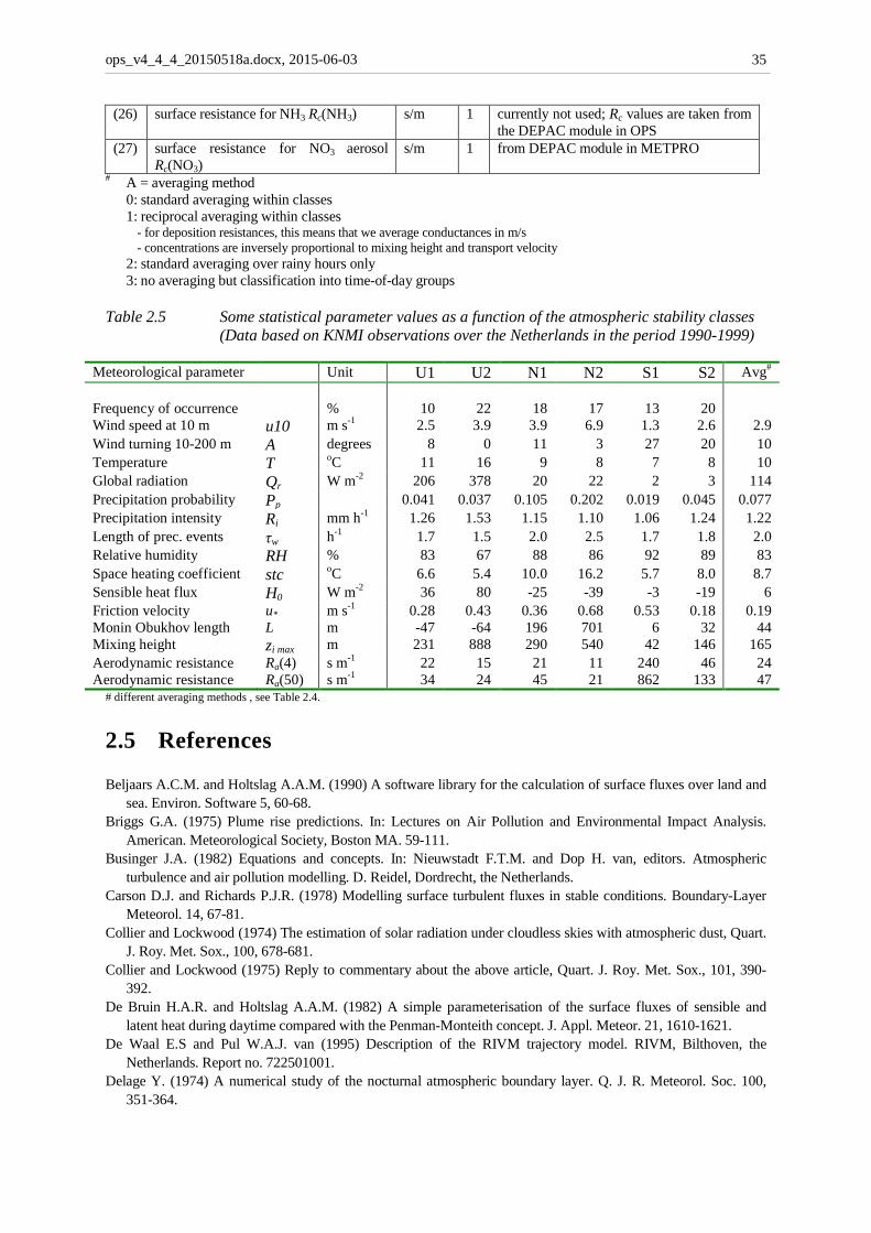
ops_v4_4_4_20150518a.docx, 2015-06-03

35

(26) surface resistance for NH3 Rc(NH3) s/m 1 currently not used; Rc values are taken from the DEPAC module in OPS

(27) surface resistance for NO3 aerosol Rc(NO3)

s/m 1 from DEPAC module in METPRO

# A = averaging method 0: standard averaging within classes 1: reciprocal averaging within classes - for deposition resistances, this means that we average conductances in m/s - concentrations are inversely proportional to mixing height and transport velocity 2: standard averaging over rainy hours only 3: no averaging but classification into time-of-day groups Table 2.5 Some statistical parameter values as a function of the atmospheric stability classes

(Data based on KNMI observations over the Netherlands in the period 1990-1999)

Meteorological parameter Unit U1 U2 N1 N2 S1 S2 Avg# Frequency of occurrence % 10 22 18 17 13 20 Wind speed at 10 m u10 m s-1 2.5 3.9 3.9 6.9 1.3 2.6 2.9 Wind turning 10-200 m A degrees 8 0 11 3 27 20 10 Temperature T oC 11 16 9 8 7 8 10 Global radiation Qr W m-2 206 378 20 22 2 3 114 Precipitation probability Pp 0.041 0.037 0.105 0.202 0.019 0.045 0.077 Precipitation intensity Ri mm h-1 1.26 1.53 1.15 1.10 1.06 1.24 1.22 Length of prec. events τw h-1 1.7 1.5 2.0 2.5 1.7 1.8 2.0 Relative humidity RH % 83 67 88 86 92 89 83 Space heating coefficient stc oC 6.6 5.4 10.0 16.2 5.7 8.0 8.7 Sensible heat flux H0 W m-2 36 80 -25 -39 -3 -19 6 Friction velocity u* m s-1 0.28 0.43 0.36 0.68 0.53 0.18 0.19 Monin Obukhov length L m -47 -64 196 701 6 32 44 Mixing height zi max m 231 888 290 540 42 146 165 Aerodynamic resistance Ra(4) s m-1 22 15 21 11 240 46 24 Aerodynamic resistance Ra(50) s m-1 34 24 45 21 862 133 47

# different averaging methods , see Table 2.4.

2.5 References Beljaars A.C.M. and Holtslag A.A.M. (1990) A software library for the calculation of surface fluxes over land and

sea. Environ. Software 5, 60-68. Briggs G.A. (1975) Plume rise predictions. In: Lectures on Air Pollution and Environmental Impact Analysis.

American. Meteorological Society, Boston MA. 59-111. Businger J.A. (1982) Equations and concepts. In: Nieuwstadt F.T.M. and Dop H. van, editors. Atmospheric

turbulence and air pollution modelling. D. Reidel, Dordrecht, the Netherlands. Carson D.J. and Richards P.J.R. (1978) Modelling surface turbulent fluxes in stable conditions. Boundary-Layer

Meteorol. 14, 67-81. Collier and Lockwood (1974) The estimation of solar radiation under cloudless skies with atmospheric dust, Quart.

J. Roy. Met. Sox., 100, 678-681. Collier and Lockwood (1975) Reply to commentary about the above article, Quart. J. Roy. Met. Sox., 101, 390-

392. De Bruin H.A.R. and Holtslag A.A.M. (1982) A simple parameterisation of the surface fluxes of sensible and

latent heat during daytime compared with the Penman-Monteith concept. J. Appl. Meteor. 21, 1610-1621. De Waal E.S and Pul W.A.J. van (1995) Description of the RIVM trajectory model. RIVM, Bilthoven, the

Netherlands. Report no. 722501001. Delage Y. (1974) A numerical study of the nocturnal atmospheric boundary layer. Q. J. R. Meteorol. Soc. 100,

351-364.

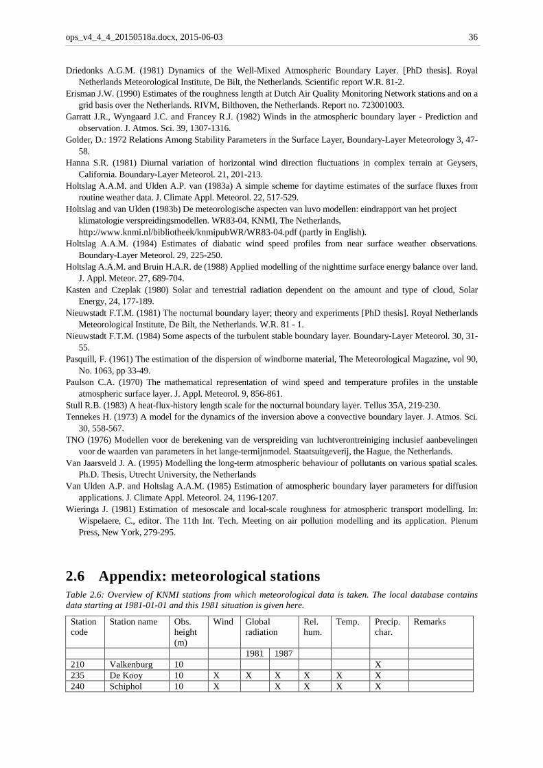
ops_v4_4_4_20150518a.docx, 2015-06-03

36

Driedonks A.G.M. (1981) Dynamics of the Well-Mixed Atmospheric Boundary Layer. [PhD thesis]. Royal Netherlands Meteorological Institute, De Bilt, the Netherlands. Scientific report W.R. 81-2.

Erisman J.W. (1990) Estimates of the roughness length at Dutch Air Quality Monitoring Network stations and on a grid basis over the Netherlands. RIVM, Bilthoven, the Netherlands. Report no. 723001003.

Garratt J.R., Wyngaard J.C. and Francey R.J. (1982) Winds in the atmospheric boundary layer - Prediction and observation. J. Atmos. Sci. 39, 1307-1316.

Golder, D.: 1972 Relations Among Stability Parameters in the Surface Layer, Boundary-Layer Meteorology 3, 47-58.

Hanna S.R. (1981) Diurnal variation of horizontal wind direction fluctuations in complex terrain at Geysers, California. Boundary-Layer Meteorol. 21, 201-213.

Holtslag A.A.M. and Ulden A.P. van (1983a) A simple scheme for daytime estimates of the surface fluxes from routine weather data. J. Climate Appl. Meteorol. 22, 517-529.

Holtslag and van Ulden (1983b) De meteorologische aspecten van luvo modellen: eindrapport van het project klimatologie verspreidingsmodellen. WR83-04, KNMI, The Netherlands, http://www.knmi.nl/bibliotheek/knmipubWR/WR83-04.pdf (partly in English).

Holtslag A.A.M. (1984) Estimates of diabatic wind speed profiles from near surface weather observations. Boundary-Layer Meteorol. 29, 225-250.

Holtslag A.A.M. and Bruin H.A.R. de (1988) Applied modelling of the nighttime surface energy balance over land. J. Appl. Meteor. 27, 689-704.

Kasten and Czeplak (1980) Solar and terrestrial radiation dependent on the amount and type of cloud, Solar Energy, 24, 177-189.

Nieuwstadt F.T.M. (1981) The nocturnal boundary layer; theory and experiments [PhD thesis]. Royal Netherlands Meteorological Institute, De Bilt, the Netherlands. W.R. 81 - 1.

Nieuwstadt F.T.M. (1984) Some aspects of the turbulent stable boundary layer. Boundary-Layer Meteorol. 30, 31-55.

Pasquill, F. (1961) The estimation of the dispersion of windborne material, The Meteorological Magazine, vol 90, No. 1063, pp 33-49.

Paulson C.A. (1970) The mathematical representation of wind speed and temperature profiles in the unstable atmospheric surface layer. J. Appl. Meteorol. 9, 856-861.

Stull R.B. (1983) A heat-flux-history length scale for the nocturnal boundary layer. Tellus 35A, 219-230. Tennekes H. (1973) A model for the dynamics of the inversion above a convective boundary layer. J. Atmos. Sci.

30, 558-567. TNO (1976) Modellen voor de berekening van de verspreiding van luchtverontreiniging inclusief aanbevelingen

voor de waarden van parameters in het lange-termijnmodel. Staatsuitgeverij, the Hague, the Netherlands. Van Jaarsveld J. A. (1995) Modelling the long-term atmospheric behaviour of pollutants on various spatial scales.

Ph.D. Thesis, Utrecht University, the Netherlands Van Ulden A.P. and Holtslag A.A.M. (1985) Estimation of atmospheric boundary layer parameters for diffusion

applications. J. Climate Appl. Meteorol. 24, 1196-1207. Wieringa J. (1981) Estimation of mesoscale and local-scale roughness for atmospheric transport modelling. In:

Wispelaere, C., editor. The 11th Int. Tech. Meeting on air pollution modelling and its application. Plenum Press, New York, 279-295.

2.6 Appendix: meteorological stations Table 2.6: Overview of KNMI stations from which meteorological data is taken. The local database contains data starting at 1981-01-01 and this 1981 situation is given here.

Station code

Station name Obs. height (m)

Wind Global radiation

Rel. hum.

Temp. Precip. char.

Remarks

1981 1987 210 Valkenburg 10 X 235 De Kooy 10 X X X X X X 240 Schiphol 10 X X X X X

ops_v4_4_4_20150518a.docx, 2015-06-03

37

250 Terschelling 10 Up to 1990 260 De Bilt 20 X X X X X X 269 Lelystad 10 270 Leeuwarden 10 X X X X X 275 Deelen 10 X X X X X 277 Lauwersoog 10 279 Hoogeveen 10 280 Eelde 10 X X X X X X 290 Twenthe 10 X X X X X 310 Vlissingen 20 X X X X X X 344 Rotterdam 10 X X X X X 348 Cabauw 10, 200 1993-1996 350 Gilze Rijen 10 X X X X X 370 Eindhoven 10 X X X X X 375 Volkel 10 X X X X 380 Maastricht 10 X X X X X X

Table 2.7: KNMI stations with snow cover data

210 235 260 270 280 290 310 370 380 1990-1995 x x x x x 1996-1999 x x x 2000-2002 x x x x x x x

From 2003, there are no snow cover data available in the LML database.

ops_v4_4_4_20150518a.docx, 2015-06-03 38

3. Mass balance and dispersion

3.1 Mass balance equations The change of a mass Mp [g] over time t [s] for a pollutant in a well-mixed layer due to chemical conversion and deposition can be formulated as follows:

M k - = dtMd

ppp (3.1)

and for a secondary-formed pollutant Ms, with linear dependence on Mp:

M k - M k = dtMd

sspcs . (3.2)

The rate constants kp and ks [s-1] are defined as:

Λ p wci

pdp + k +

zv = k (3.3)

Λ swi

sds +

zv = k , (3.4)

where vdp and vds are dry deposition velocities [m s-1], Λwp and Λws wet scavenging coefficients [s-1], kc the pseudo first-order chemical reaction constant [s-1], and zi the mixing-layer height [m]. Subscripts p and s refer to the primary-emitted and the secondary-formed substance respectively. Further chemical reactions involving Ms are not taken into account. The cross-wind integrated mass flux Q [g s-1] at a distance x [m] from the point of release for a source emitting continuously with a rate of Q0 [g s-1] can be obtained by solving Eqs. (3.1) and (3.2) after introduction of a horizontal transport velocity u [m s-1] (u = x/t):

)(expux k- Q = (x) Q p0p (3.5)

)(exp)(exp

ux k- -

ux k-

k - kk Q = (x) Q ps

sp

c0s . (3.6)

38

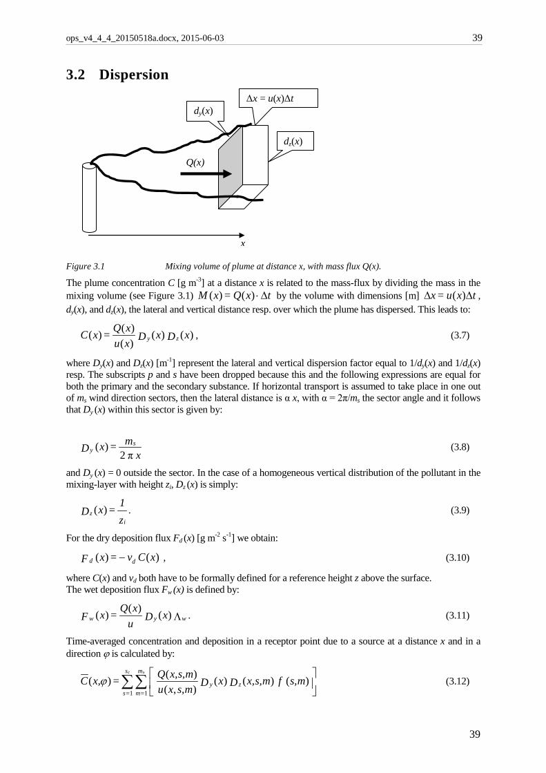
ops_v4_4_4_20150518a.docx, 2015-06-03 39

3.2 Dispersion

Figure 3.1 Mixing volume of plume at distance x, with mass flux Q(x).

The plume concentration C [g m-3] at a distance x is related to the mass-flux by dividing the mass in the mixing volume (see Figure 3.1) txQ= xM ∆⋅)()( by the volume with dimensions [m] txu= x ∆∆ )( , dy(x), and dz(x), the lateral and vertical distance resp. over which the plume has dispersed. This leads to:

)()()()()( xD xD xu

xQ = xC zy , (3.7)

where Dy(x) and Dz(x) [m-1] represent the lateral and vertical dispersion factor equal to 1/dy(x) and 1/dz(x) resp. The subscripts p and s have been dropped because this and the following expressions are equal for both the primary and the secondary substance. If horizontal transport is assumed to take place in one out of ms wind direction sectors, then the lateral distance is α x, with α = 2π/ms the sector angle and it follows that Dy (x) within this sector is given by:

x

m = x D sy π2

)( (3.8)

and Dy (x) = 0 outside the sector. In the case of a homogeneous vertical distribution of the pollutant in the mixing-layer with height zi, Dz (x) is simply:

z1 =xD

iz )( . (3.9)

For the dry deposition flux Fd (x) [g m-2 s-1] we obtain:

)()( xCv = x F dd − , (3.10)

where C(x) and vd both have to be formally defined for a reference height z above the surface. The wet deposition flux Fw (x) is defined by:

Λwyw xD uxQ = x F )()()( . (3.11)

Time-averaged concentration and deposition in a receptor point due to a source at a distance x and in a direction ϕ is calculated by:

∑∑ ms, fms,x,D xD ms,xums,x,Q = x,C zy

m

=m

s

=s

sc

)( )()(),()()(

11

ϕ (3.12)

x

Q(x)

Δx = u(x)Δt

dz(x)

dy(x)

39

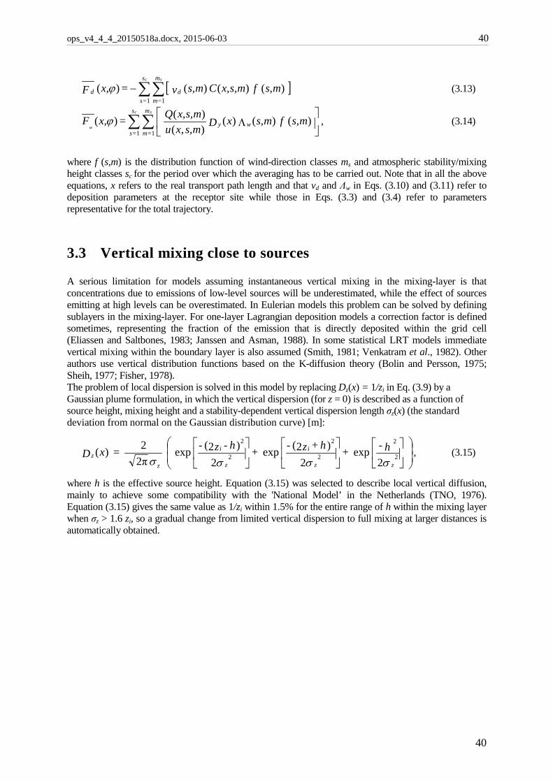
ops_v4_4_4_20150518a.docx, 2015-06-03 40

[ ] ms, f ms,x,C ms, v = x, F d

m

=m

s

=sd

sc

)()()()(11∑∑−ϕ (3.13)

Λ∑∑ ms, f ms, xD ms,xu

ms,x,Q =x,F wy

m

=m

s

=s

sc

w)()()(

),()( )(

11

ϕ , (3.14)

where f (s,m) is the distribution function of wind-direction classes ms and atmospheric stability/mixing height classes sc for the period over which the averaging has to be carried out. Note that in all the above equations, x refers to the real transport path length and that vd and Λw in Eqs. (3.10) and (3.11) refer to deposition parameters at the receptor site while those in Eqs. (3.3) and (3.4) refer to parameters representative for the total trajectory.

3.3 Vertical mixing close to sources A serious limitation for models assuming instantaneous vertical mixing in the mixing-layer is that concentrations due to emissions of low-level sources will be underestimated, while the effect of sources emitting at high levels can be overestimated. In Eulerian models this problem can be solved by defining sublayers in the mixing-layer. For one-layer Lagrangian deposition models a correction factor is defined sometimes, representing the fraction of the emission that is directly deposited within the grid cell (Eliassen and Saltbones, 1983; Janssen and Asman, 1988). In some statistical LRT models immediate vertical mixing within the boundary layer is also assumed (Smith, 1981; Venkatram et al., 1982). Other authors use vertical distribution functions based on the K-diffusion theory (Bolin and Persson, 1975; Sheih, 1977; Fisher, 1978). The problem of local dispersion is solved in this model by replacing Dz(x) = 1/zi in Eq. (3.9) by a Gaussian plume formulation, in which the vertical dispersion (for z = 0) is described as a function of source height, mixing height and a stability-dependent vertical dispersion length σz(x) (the standard deviation from normal on the Gaussian distribution curve) [m]:

h- + h+z- + h-z-

= xD

z

z

i

z

i

zz

σσσσ 2exp

2)2(exp

2)2(exp

2π2)( 2

2

2

2

2

2

, (3.15)

where h is the effective source height. Equation (3.15) was selected to describe local vertical diffusion, mainly to achieve some compatibility with the 'National Model’ in the Netherlands (TNO, 1976). Equation (3.15) gives the same value as 1/zi within 1.5% for the entire range of h within the mixing layer when σz > 1.6 zi, so a gradual change from limited vertical dispersion to full mixing at larger distances is automatically obtained.

40

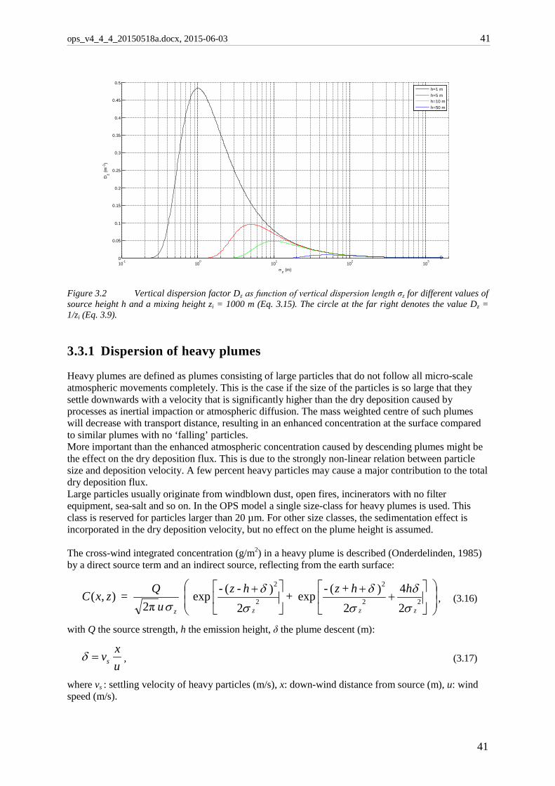
ops_v4_4_4_20150518a.docx, 2015-06-03 41

10-1

100

101

102

103

0

0.05

0.1

0.15

0.2

0.25

0.3

0.35

0.4

0.45

0.5

σz (m)

Dz (m

-1)

h=1 mh=5 mh=10 mh=50 m

Figure 3.2 Vertical dispersion factor Dz as function of vertical dispersion length σz for different values of source height h and a mixing height zi = 1000 m (Eq. 3.15). The circle at the far right denotes the value Dz = 1/zi (Eq. 3.9).

3.3.1 Dispersion of heavy plumes Heavy plumes are defined as plumes consisting of large particles that do not follow all micro-scale atmospheric movements completely. This is the case if the size of the particles is so large that they settle downwards with a velocity that is significantly higher than the dry deposition caused by processes as inertial impaction or atmospheric diffusion. The mass weighted centre of such plumes will decrease with transport distance, resulting in an enhanced concentration at the surface compared to similar plumes with no ‘falling’ particles. More important than the enhanced atmospheric concentration caused by descending plumes might be the effect on the dry deposition flux. This is due to the strongly non-linear relation between particle size and deposition velocity. A few percent heavy particles may cause a major contribution to the total dry deposition flux. Large particles usually originate from windblown dust, open fires, incinerators with no filter equipment, sea-salt and so on. In the OPS model a single size-class for heavy plumes is used. This class is reserved for particles larger than 20 µm. For other size classes, the sedimentation effect is incorporated in the dry deposition velocity, but no effect on the plume height is assumed. The cross-wind integrated concentration (g/m2) in a heavy plume is described (Onderdelinden, 1985) by a direct source term and an indirect source, reflecting from the earth surface:

+

+

+ hh+z- + h-z- u

Q = zxCzzzz σδ

σδ

σδ

σ 24

2)(exp

2)(exp

2π),( 22

2

2

2

, (3.16)

with Q the source strength, h the emission height, δ the plume descent (m):

uxvs=δ , (3.17)

where vs : settling velocity of heavy particles (m/s), x: down-wind distance from source (m), u: wind speed (m/s).

41

ops_v4_4_4_20150518a.docx, 2015-06-03 42

3.3.2 Local vertical dispersion For an appropriate determination of the vertical dispersion length, the turbulent state of the atmospheric boundary layer must be assessed. Most widely used is the approach of Pasquill (1961) and Gifford (1961). The Pasquill-Gifford scheme prescribes the quantitative relation between the stability of the atmosphere and insulation in combination with wind speed. The scheme has been deduced from experiments using sources near the ground. First versions of the present model (Van Jaarsveld, 1990) also used the Pasquill-Gifford scheme for dispersion and an empirical method for estimating stability similar to the Pasquill-Turner scheme (KNMI, 1972). Vertical dispersion was described there as

bzz xac 0=σ , (3.18)

with cz0 a correction factor for surface roughness and a and b stability-class-dependent dispersion coefficients taken from the Dutch National model (TNO, 1976).

Table 3.1: initial settings of parameters a and b in Eq. 3.18. Note that coefficient a is recalculated based on more sophisticated parameterisations of σz .

Figure 3.3 Vertical dispersion length σz as described by Pasquill as function of x = distance from source, for stability classes {U1, U2}, {N1, N2, S2} and S1; cz0 = 1. Stability classes as defined in Table 1.1. Note that the present OPS-model uses more sophisticated parameterisations of σz .

Turbulence typing schemes, such as the Pasquill-Turner one, are biased toward neutral stability when convective situations actually exist (Weil and Brower, 1984). Kretzschmar and Mertens (1984) reviewed the turbulence typing schemes and corresponding dispersion algorithms of a number of Gaussian short-range models. They found that the predicted maximum concentration and also the distance of this maximum concentration differed between the models by one order of magnitude. In the present version of the model, more recent concepts of the description of turbulence and dispersion in the boundary layer have been used. In such a concept the boundary layer is divided into a number of regimes, each characterised by distinct scaling parameters (Holtslag and Nieuwstadt, 1986; Gryning et al., 1987). The Holtslag and Nieuwstadt scheme is adopted here in a simplified form. The regimes distinguished are (see also Figure 3.4): a. a surface layer with a height up to 0.1 zi, b. a convective mixing layer (zi /L < -10 and z/zi > 0.1) c. a near neutral upper layer (0 > zi /L > -10 and z/zi > 0.1) and d. a second near neutral layer above a stable surface layer (0 < zi /L and z/zi > 0.1), where L is the Monin-Obukhov length [m].

stability class a b

U1, U2 0.2800 0.8200

N1, N2, S2 0.2000 0.7600

S1 0.1200 0.6700 0 10 20 30 40 50 60 70 80 90 1000

500

1000

1500

2000

2500

3000

3500

4000

x (km)

σz (

m)

U1, U2N1, N2, S2S1

42

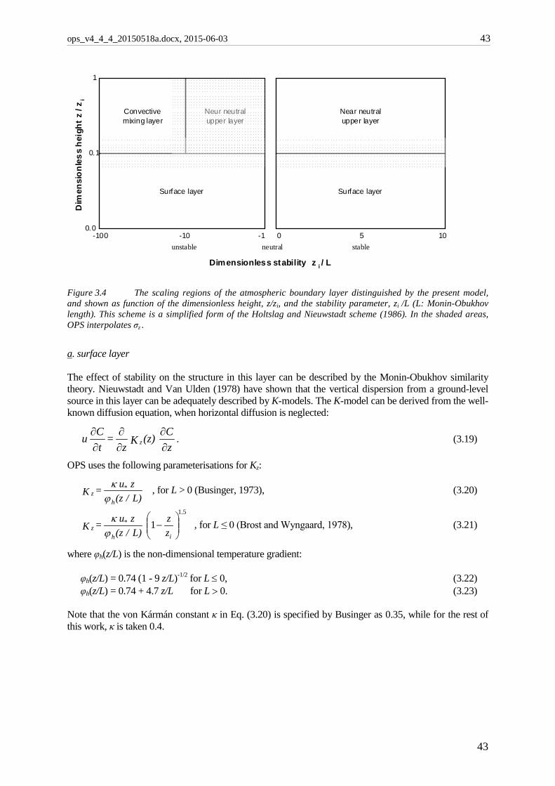
ops_v4_4_4_20150518a.docx, 2015-06-03 43

Surface layer Surface layer

Convectivemixing layer

Neur neutralupper layer

Near neutralupper layer

-100 -1 0 105-10

Dimensionless stability z i / L

Dim

ensi

onle

ss h

eigh

t z /

z i

0.0

0.1

1

neutralunstable stable

Figure 3.4 The scaling regions of the atmospheric boundary layer distinguished by the present model, and shown as function of the dimensionless height, z/zi, and the stability parameter, zi /L (L: Monin-Obukhov length). This scheme is a simplified form of the Holtslag and Nieuwstadt scheme (1986). In the shaded areas, OPS interpolates σz .

a. surface layer The effect of stability on the structure in this layer can be described by the Monin-Obukhov similarity theory. Nieuwstadt and Van Ulden (1978) have shown that the vertical dispersion from a ground-level source in this layer can be adequately described by K-models. The K-model can be derived from the well-known diffusion equation, when horizontal diffusion is neglected:

zC (z)K z

= tCu z ∂

∂∂∂

∂∂

. (3.19)

OPS uses the following parameterisations for Kz:

L) /(z z u = K

hz ϕ

κ * , for L > 0 (Businger, 1973), (3.20)

zz

L) /(z z u = K

ihz

5.1* 1

−

ϕκ , for L ≤ 0 (Brost and Wyngaard, 1978), (3.21)

where φh(z/L) is the non-dimensional temperature gradient: φh(z/L) = 0.74 (1 - 9 z/L)-1/2 for L ≤ 0, (3.22) φh(z/L) = 0.74 + 4.7 z/L for L > 0. (3.23) Note that the von Kármán constant κ in Eq. (3.20) is specified by Businger as 0.35, while for the rest of this work, κ is taken 0.4.

43

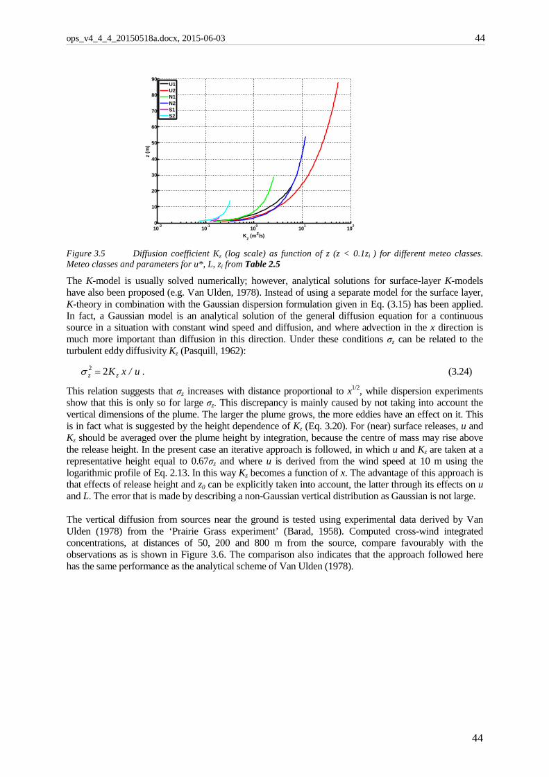
ops_v4_4_4_20150518a.docx, 2015-06-03 44

10-2 10-1 100 101 1020

10

20

30

40

50

60

70

80

90

Kz (m2/s)

z (m

)

U1U2N1N2S1S2

Figure 3.5 Diffusion coefficient Kz (log scale) as function of z (z < 0.1zi ) for different meteo classes. Meteo classes and parameters for u*, L, zi from Table 2.5

The K-model is usually solved numerically; however, analytical solutions for surface-layer K-models have also been proposed (e.g. Van Ulden, 1978). Instead of using a separate model for the surface layer, K-theory in combination with the Gaussian dispersion formulation given in Eq. (3.15) has been applied. In fact, a Gaussian model is an analytical solution of the general diffusion equation for a continuous source in a situation with constant wind speed and diffusion, and where advection in the x direction is much more important than diffusion in this direction. Under these conditions σz can be related to the turbulent eddy diffusivity Kz (Pasquill, 1962):

u / xKzz 22 =σ . (3.24)

This relation suggests that σz increases with distance proportional to x1/2, while dispersion experiments show that this is only so for large σz. This discrepancy is mainly caused by not taking into account the vertical dimensions of the plume. The larger the plume grows, the more eddies have an effect on it. This is in fact what is suggested by the height dependence of Kz (Eq. 3.20). For (near) surface releases, u and Kz should be averaged over the plume height by integration, because the centre of mass may rise above the release height. In the present case an iterative approach is followed, in which u and Kz are taken at a representative height equal to 0.67σz and where u is derived from the wind speed at 10 m using the logarithmic profile of Eq. 2.13. In this way Kz becomes a function of x. The advantage of this approach is that effects of release height and z0 can be explicitly taken into account, the latter through its effects on u and L. The error that is made by describing a non-Gaussian vertical distribution as Gaussian is not large. The vertical diffusion from sources near the ground is tested using experimental data derived by Van Ulden (1978) from the ‘Prairie Grass experiment’ (Barad, 1958). Computed cross-wind integrated concentrations, at distances of 50, 200 and 800 m from the source, compare favourably with the observations as is shown in Figure 3.6. The comparison also indicates that the approach followed here has the same performance as the analytical scheme of Van Ulden (1978).

44

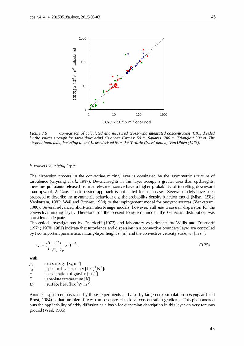
ops_v4_4_4_20150518a.docx, 2015-06-03 45

1

10

100

1000

1 10 100 1000

CIC/Q x 10-3 s m-2 observed

CIC

/Q x

10-3

s m

-2 c

alcu

late

d

Figure 3.6 Comparison of calculated and measured cross-wind integrated concentration (CIC) divided by the source strength for three down-wind distances. Circles: 50 m. Squares: 200 m. Triangles: 800 m. The observational data, including u* and L, are derived from the ‘Prairie Grass’ data by Van Ulden (1978).

b. convective mixing layer The dispersion process in the convective mixing layer is dominated by the asymmetric structure of turbulence (Gryning et al., 1987). Downdraughts in this layer occupy a greater area than updraughts; therefore pollutants released from an elevated source have a higher probability of travelling downward than upward. A Gaussian dispersion approach is not suited for such cases. Several models have been proposed to describe the asymmetric behaviour e.g. the probability density function model (Misra, 1982; Venkatram, 1983; Weil and Brower, 1984) or the impingement model for buoyant sources (Venkatram, 1980). Several advanced short-term short-range models, however, still use Gaussian dispersion for the convective mixing layer. Therefore for the present long-term model, the Gaussian distribution was considered adequate. Theoretical investigations by Deardorff (1972) and laboratory experiments by Willis and Deardorff (1974; 1978; 1981) indicate that turbulence and dispersion in a convective boundary layer are controlled by two important parameters: mixing-layer height zi [m] and the convective velocity scale, w* [m s-1]:

)( 1/3 z c

H Tg = w i

pa

0* ρ

, (3.25)

with ρa : air density [kg m-3] cp : specific heat capacity [J kg-1 K-1]/ g : acceleration of gravity [m s-2] T : absolute temperature [K] H0 : surface heat flux [W m-2]. Another aspect demonstrated by these experiments and also by large eddy simulations (Wyngaard and Brost, 1984) is that turbulent fluxes can be opposed to local concentration gradients. This phenomenon puts the applicability of eddy diffusion as a basis for dispersion description in this layer on very tenuous ground (Weil, 1985).

45

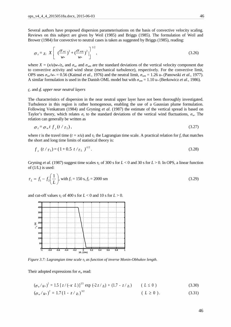
ops_v4_4_4_20150518a.docx, 2015-06-03 46

Several authors have proposed dispersion parameterisations on the basis of convective velocity scaling. Reviews on this subject are given by Weil (1985) and Briggs (1985). The formulation of Weil and Brower (1984) for convective to neutral cases is taken as suggested by Briggs (1985), reading:

w

+ w

X z = *

wm

*

wc

iz )()( 221/2

σσσ , (3.26)

where X = (x/u)w*/zi, and σwc and σwm are the standard deviations of the vertical velocity component due to convective activity and wind shear (mechanical turbulence), respectively. For the convective limit, OPS uses σwc/w* = 0.56 (Kaimal et al., 1976) and the neutral limit, σwm = 1.26 u* (Panowski et al., 1977). A similar formulation is used in the Danish OML model but with σwm = 1.10 u* (Berkowicz et al., 1986). c. and d. upper near neutral layers The characteristics of dispersion in the near neutral upper layer have not been thoroughly investigated. Turbulence in this region is rather homogenous, enabling the use of a Gaussian plume formulation. Following Venkatram (1984) and Gryning et al. (1987) the estimate of the vertical spread is based on Taylor’s theory, which relates σz to the standard deviations of the vertical wind fluctuations, σw. The relation can generally be written as

)( τσσ Lzwz / t f t = , (3.27)

where t is the travel time (t = x/u) and τL the Lagrangian time scale. A practical relation for fz that matches the short and long time limits of statistical theory is:

) / t = / t f -LLz

1/20.5 + 1 ()( ττ . (3.28)

Gryning et al. (1987) suggest time scales τL of 300 s for L < 0 and 30 s for L > 0. In OPS, a linear function of (1/L) is used:

−=

LffL

121τ , with f1 = 150 s, f2 = 2000 sm (3.29)

and cut-off values τL of 400 s for L < 0 and 10 s for L > 0.

-1 -0.8 -0.6 -0.4 -0.2 0 0.2 0.4 0.6 0.8 10

50

100

150

200

250

300

350

400

450

1/L (1/m)

τ L (s

)

Figure 3.7: Lagrangian time scale τL as function of inverse Monin-Obhukov length.

Their adopted expressions for σw read:

) 0 ( )(1.7 )2(exp])( [ 1.5 )( 2/3 2 ≤L z /z - + z /z - L - /z = u/ ii*w κσ (3.30)

) 0 ( ) 1 ( 1.7)( 3/2 2 ≥L z /z - = u/ i*wσ . (3.31)

46

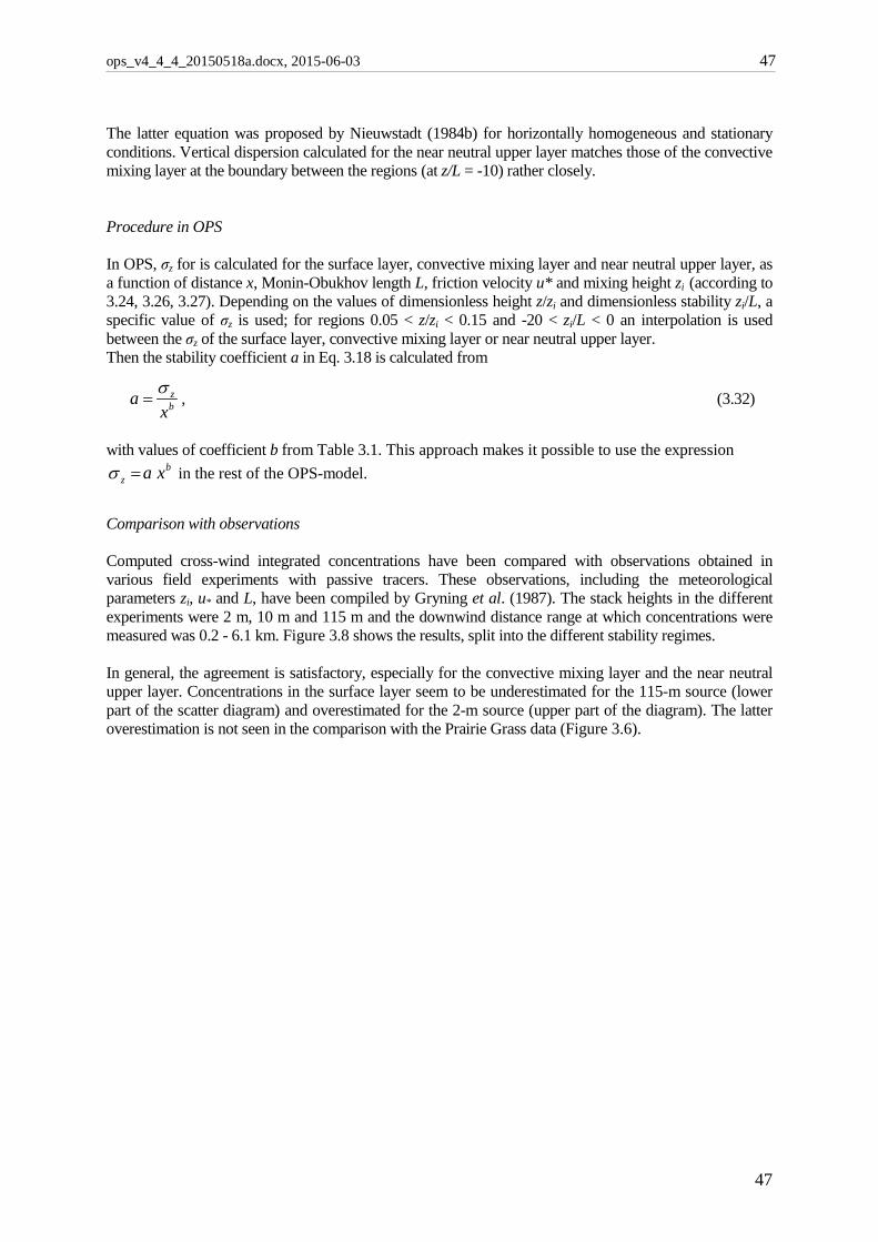
ops_v4_4_4_20150518a.docx, 2015-06-03 47

The latter equation was proposed by Nieuwstadt (1984b) for horizontally homogeneous and stationary conditions. Vertical dispersion calculated for the near neutral upper layer matches those of the convective mixing layer at the boundary between the regions (at z/L = -10) rather closely. Procedure in OPS In OPS, σz for is calculated for the surface layer, convective mixing layer and near neutral upper layer, as a function of distance x, Monin-Obukhov length L, friction velocity u* and mixing height zi (according to 3.24, 3.26, 3.27). Depending on the values of dimensionless height z/zi and dimensionless stability zi/L, a specific value of σz is used; for regions 0.05 < z/zi < 0.15 and -20 < zi/L < 0 an interpolation is used between the σz of the surface layer, convective mixing layer or near neutral upper layer. Then the stability coefficient a in Eq. 3.18 is calculated from

bz

xa σ= , (3.32)

with values of coefficient b from Table 3.1. This approach makes it possible to use the expression

bz xa=σ in the rest of the OPS-model.

Comparison with observations Computed cross-wind integrated concentrations have been compared with observations obtained in various field experiments with passive tracers. These observations, including the meteorological parameters zi, u* and L, have been compiled by Gryning et al. (1987). The stack heights in the different experiments were 2 m, 10 m and 115 m and the downwind distance range at which concentrations were measured was 0.2 - 6.1 km. Figure 3.8 shows the results, split into the different stability regimes. In general, the agreement is satisfactory, especially for the convective mixing layer and the near neutral upper layer. Concentrations in the surface layer seem to be underestimated for the 115-m source (lower part of the scatter diagram) and overestimated for the 2-m source (upper part of the diagram). The latter overestimation is not seen in the comparison with the Prairie Grass data (Figure 3.6).

47

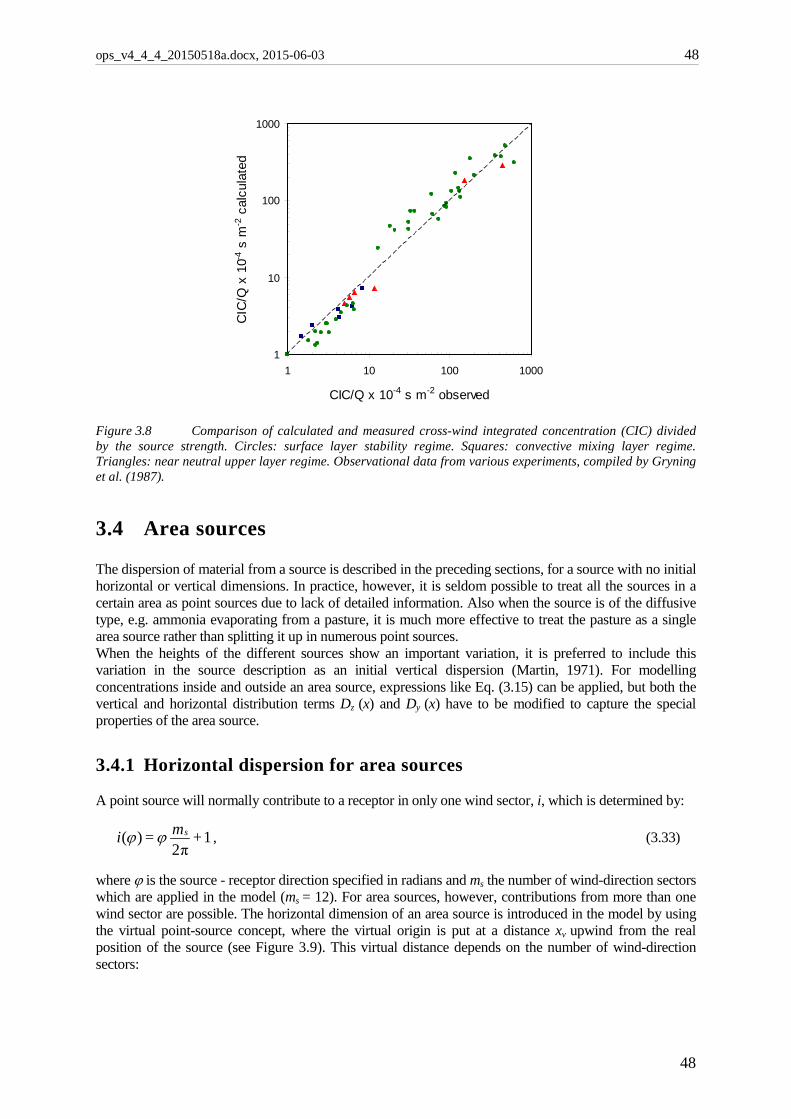
ops_v4_4_4_20150518a.docx, 2015-06-03 48

1

10

100

1000

1 10 100 1000

CIC/Q x 10-4 s m-2 observed

CIC

/Q x

10-4

s m

-2 c

alcu

late

d

Figure 3.8 Comparison of calculated and measured cross-wind integrated concentration (CIC) divided by the source strength. Circles: surface layer stability regime. Squares: convective mixing layer regime. Triangles: near neutral upper layer regime. Observational data from various experiments, compiled by Gryning et al. (1987).

3.4 Area sources The dispersion of material from a source is described in the preceding sections, for a source with no initial horizontal or vertical dimensions. In practice, however, it is seldom possible to treat all the sources in a certain area as point sources due to lack of detailed information. Also when the source is of the diffusive type, e.g. ammonia evaporating from a pasture, it is much more effective to treat the pasture as a single area source rather than splitting it up in numerous point sources. When the heights of the different sources show an important variation, it is preferred to include this variation in the source description as an initial vertical dispersion (Martin, 1971). For modelling concentrations inside and outside an area source, expressions like Eq. (3.15) can be applied, but both the vertical and horizontal distribution terms Dz (x) and Dy (x) have to be modified to capture the special properties of the area source.

3.4.1 Horizontal dispersion for area sources A point source will normally contribute to a receptor in only one wind sector, i, which is determined by:

1π2

)( + m = i sϕϕ , (3.33)

where ϕ is the source - receptor direction specified in radians and ms the number of wind-direction sectors which are applied in the model (ms = 12). For area sources, however, contributions from more than one wind sector are possible. The horizontal dimension of an area source is introduced in the model by using the virtual point-source concept, where the virtual origin is put at a distance xv upwind from the real position of the source (see Figure 3.9). This virtual distance depends on the number of wind-direction sectors:

48

ops_v4_4_4_20150518a.docx, 2015-06-03 49

π2πr ms m = x asas

v = , (3.34)

where sa is the diameter of the source and ra its radius. Replacing x by (x + xv) in Eq. (3.8) introduces the effect of the horizontal dimensions of the source into the description of the horizontal dispersion.

s a

xv x

R cp30 o• •

Figure 3.9 Area source represented by a virtual point source.

Another part of the problem is that an area source contributes more often to a given receptor point than a point source does. This is illustrated in Figure 3.10.

s a

x

R cp

30 o

φ

30 o

l

l

l

Figure 3.10 Wind directions for which an area source contributes to the concentration in a receptor

point. The wind direction angle, for which influence from the area source to concentrations in a receptor point

Rcp can be expected, is indicated by φ. Since π121π

21

2

−=−

sm = αγ , =)

STTR

arctan( cp= δ

))(

arctan(22

rrx

a

a− and π2

1 = δγϕ ++ , it follows that

S

T

β

α

γ δ φ

49

ops_v4_4_4_20150518a.docx, 2015-06-03 50

.π121)

)(arctan(2π2

22

mr

rx

sa

a

−+

−−=ϕ (3.35)

An equivalent formulation uses )arcsin()SRSTarcsin(

cp xr= a=β and π

2π

21 =

−++ βγϕ :

.)arcsin(2π2 xr

m a

s

+=ϕ (3.36)

We consider n contributing wind sectors, with

( ) m = n

sπ2ϕ

. (3.37)

For very large distances (x → ∞), n approaches 1, so an area source at that distance is seen as a point source. Another extreme case is when the receptor point is at the edge of the area source (x = ra); the number of sectors then becomes: n = 1 + ms /2, which means that using a classification in 12 sectors, the contributions of 7 wind-direction sectors have to be accumulated in determining an average concen-tration. Equation (3.37) is applied for x down to ra , where the contribution of the 7 sectors is weighed according to the distance to the central sector (sector upwind from the direction centre of the area source to the receptor). The maximum of seven contributing sectors is also applied for receptors within the area source.

3.4.2 Vertical dispersion for area sources The virtual point source concept, as used for the description of horizontal dispersion from sources with non-zero horizontal dimensions, is in principle also suitable for the description of vertical dispersion if plumes have initial vertical dimensions. The corresponding virtual distance would then of course differ from xv given in Eq. (3.34). The vertical plume dimension of a source with non-zero horizontal dimensions cannot be described by the virtual point source concept because Dz (x) is a non-linear function of x. In the following, an effective vertical dispersion parameter is derived which is used in the equation for Dz (x). If one considers an area source as a source representing an infinite number of point sources, then the effective vertical distribution term at a distance x down-wind from the centre of the area source can be written as (see Figure 3.11):

0)()(1)( 112

2

1

rdr rD r - r

= xDr

rzeffz ≥∫ , (3.38)

where Dz(r) is the vertical distribution term for a point source at distance r down-wind as given by Eq. (3.15). r1 is taken as zero when r < ½ sa .

50

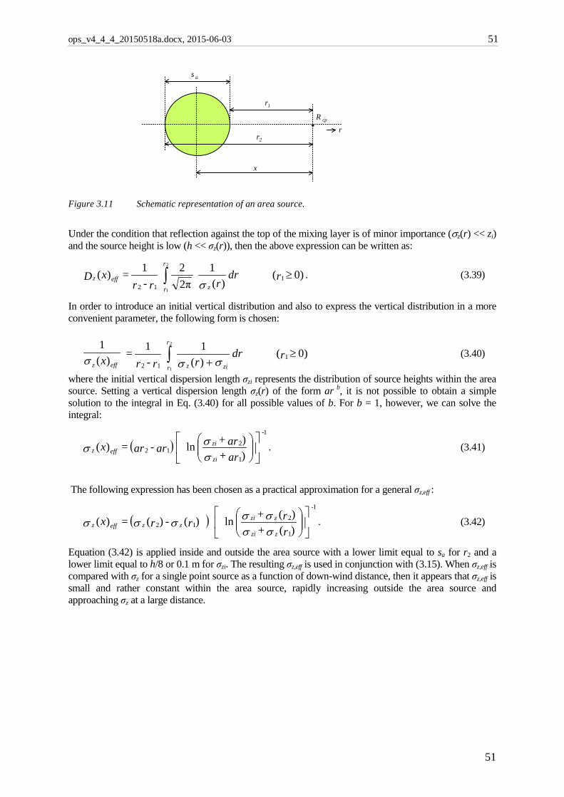
ops_v4_4_4_20150518a.docx, 2015-06-03 51

s a

r2

x

R cp

r1

r

Figure 3.11 Schematic representation of an area source.

Under the condition that reflection against the top of the mixing layer is of minor importance (σz(r) << zi) and the source height is low (h << σz(r)), then the above expression can be written as:

0)()(

12π21)( 1

12

2

1

rdr r

r - r

= xDz

r

reffz ≥∫ σ

. (3.39)

In order to introduce an initial vertical distribution and also to express the vertical distribution in a more convenient parameter, the following form is chosen:

0)()(11

)(1

112

2

1

rdr r

r - r

= x ziz

r

reffz≥

+∫ σσσ (3.40)

where the initial vertical dispersion length σzi represents the distribution of source heights within the area source. Setting a vertical dispersion length σz(r) of the form ar b, it is not possible to obtain a simple solution to the integral in Eq. (3.40) for all possible values of b. For b = 1, however, we can solve the integral:

( )

ar + ar + ar - ar = x

zi

zi

effz ))ln)(

1

2

1-

12σσσ . (3.41)

The following expression has been chosen as a practical approximation for a general σz,eff :

( )

r + r + r - r = x

zzi

zzi

zzeffz )()(ln)()()(

1

2

1-

12σσσσσσσ . (3.42)

Equation (3.42) is applied inside and outside the area source with a lower limit equal to sa for r2 and a lower limit equal to h/8 or 0.1 m for σzi. The resulting σz,eff is used in conjunction with (3.15). When σz,eff is compared with σz for a single point source as a function of down-wind distance, then it appears that σz,eff is small and rather constant within the area source, rapidly increasing outside the area source and approaching σz at a large distance.

51

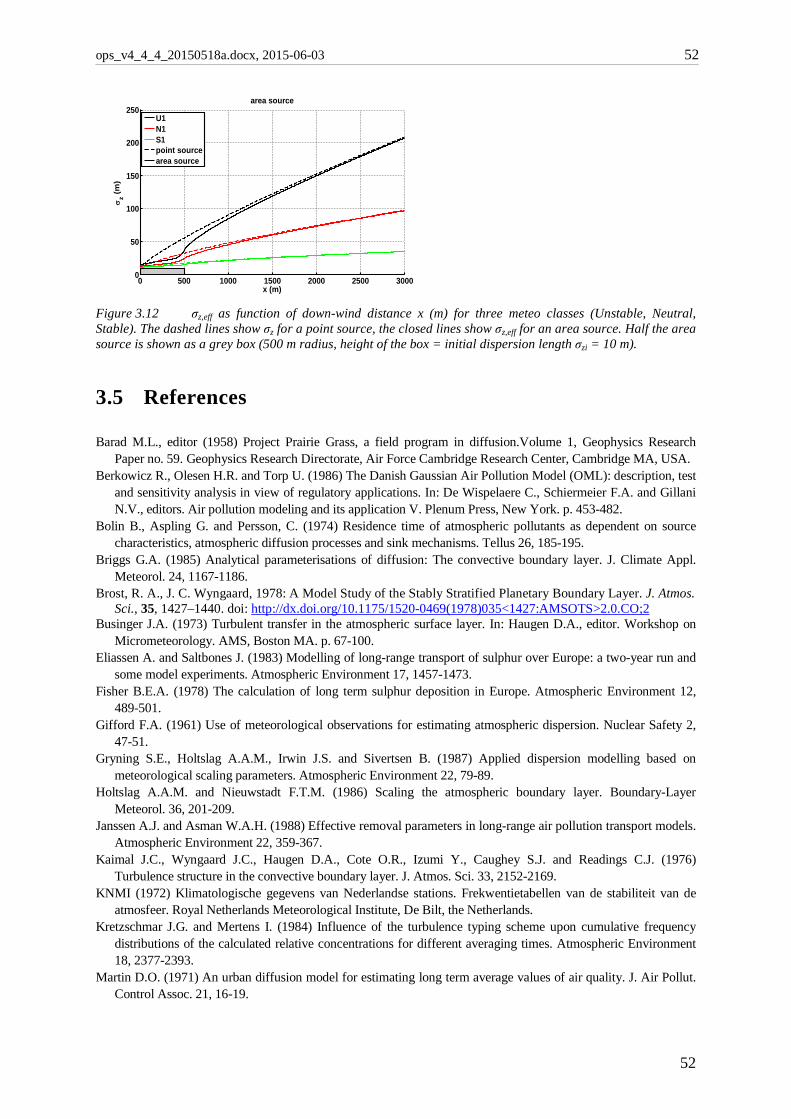
ops_v4_4_4_20150518a.docx, 2015-06-03 52

0 500 1000 1500 2000 2500 30000

50

100

150

200

250

x (m)

σz (m

)

area source

U1N1S1point sourcearea source

Figure 3.12 σz,eff as function of down-wind distance x (m) for three meteo classes (Unstable, Neutral, Stable). The dashed lines show σz for a point source, the closed lines show σz,eff for an area source. Half the area source is shown as a grey box (500 m radius, height of the box = initial dispersion length σzi = 10 m).

3.5 References Barad M.L., editor (1958) Project Prairie Grass, a field program in diffusion.Volume 1, Geophysics Research

Paper no. 59. Geophysics Research Directorate, Air Force Cambridge Research Center, Cambridge MA, USA. Berkowicz R., Olesen H.R. and Torp U. (1986) The Danish Gaussian Air Pollution Model (OML): description, test

and sensitivity analysis in view of regulatory applications. In: De Wispelaere C., Schiermeier F.A. and Gillani N.V., editors. Air pollution modeling and its application V. Plenum Press, New York. p. 453-482.

Bolin B., Aspling G. and Persson, C. (1974) Residence time of atmospheric pollutants as dependent on source characteristics, atmospheric diffusion processes and sink mechanisms. Tellus 26, 185-195.

Briggs G.A. (1985) Analytical parameterisations of diffusion: The convective boundary layer. J. Climate Appl. Meteorol. 24, 1167-1186.

Brost, R. A., J. C. Wyngaard, 1978: A Model Study of the Stably Stratified Planetary Boundary Layer. J. Atmos. Sci., 35, 1427–1440. doi: http://dx.doi.org/10.1175/1520-0469(1978)035<1427:AMSOTS>2.0.CO;2

Businger J.A. (1973) Turbulent transfer in the atmospheric surface layer. In: Haugen D.A., editor. Workshop on Micrometeorology. AMS, Boston MA. p. 67-100.

Eliassen A. and Saltbones J. (1983) Modelling of long-range transport of sulphur over Europe: a two-year run and some model experiments. Atmospheric Environment 17, 1457-1473.

Fisher B.E.A. (1978) The calculation of long term sulphur deposition in Europe. Atmospheric Environment 12, 489-501.

Gifford F.A. (1961) Use of meteorological observations for estimating atmospheric dispersion. Nuclear Safety 2, 47-51.

Gryning S.E., Holtslag A.A.M., Irwin J.S. and Sivertsen B. (1987) Applied dispersion modelling based on meteorological scaling parameters. Atmospheric Environment 22, 79-89.

Holtslag A.A.M. and Nieuwstadt F.T.M. (1986) Scaling the atmospheric boundary layer. Boundary-Layer Meteorol. 36, 201-209.

Janssen A.J. and Asman W.A.H. (1988) Effective removal parameters in long-range air pollution transport models. Atmospheric Environment 22, 359-367.

Kaimal J.C., Wyngaard J.C., Haugen D.A., Cote O.R., Izumi Y., Caughey S.J. and Readings C.J. (1976) Turbulence structure in the convective boundary layer. J. Atmos. Sci. 33, 2152-2169.

KNMI (1972) Klimatologische gegevens van Nederlandse stations. Frekwentietabellen van de stabiliteit van de atmosfeer. Royal Netherlands Meteorological Institute, De Bilt, the Netherlands.

Kretzschmar J.G. and Mertens I. (1984) Influence of the turbulence typing scheme upon cumulative frequency distributions of the calculated relative concentrations for different averaging times. Atmospheric Environment 18, 2377-2393.

Martin D.O. (1971) An urban diffusion model for estimating long term average values of air quality. J. Air Pollut. Control Assoc. 21, 16-19.

52

ops_v4_4_4_20150518a.docx, 2015-06-03 53

Misra P.K. (1982) Dispersion of non-buoyant particles inside a convective boundary layer. Atmospheric Environment 16, 239-243.

Nieuwstadt F.T.M. (1984b) The turbulent structure of the stable nocturnal boundary layer. J. Atmos. Sci. 41, 2202-2216.

Nieuwstadt F.T.M. and Ulden A.P. van (1978) A numerical study on the vertical dispersion of passive contaminants from a continuous source in the atmospheric surface layer. Atmospheric Environment 12, 2119-2124.

Onderdelinden (1985): Source depletion model, personal communication in OPS archive. Panowski H.A. Tennekes H., Lenschow D.H. and Wyngaard J.C. (1977) The characteristics of turbulence velocity

components in the surface layer under convective conditions. Boundary-Layer Meteorol. 11, 355-361. Pasquill F. (1961) The estimation of the dispersion of windborn material. Meteorol. Mag. 90, 33-49. Pasquill F. (1962) Atmospheric Diffusion. Van Nostrand, New York. p. 77. Sheih C.M. (1977) Application of a statistical trajectory model to the simulation of sulfur pollution over

northeastern United States. Atmospheric Environment 11, 173-178. Smith F.B. (1981) The significance of wet and dry synoptic regions on long-range transport of pollution and its

deposition. Atmospheric Environment 15, 863-873. TNO (1976) Modellen voor de berekening van de verspreiding van luchtverontreiniging inclusief aanbevelingen

voor de waarden van parameters in het lange-termijnmodel. Staatsuitgeverij, The Hague, the Netherlands. Van Jaarsveld J.A. (1990) An operational atmospheric transport model for priority substances; specification and

instructions for use. RIVM, Bilthoven, the Netherlands. Report no. 222501002. Venkatram A. (1980) Dispersion from an elevated source in a convective boundary layer. Atmospheric

Environment 14, 1-10. Venkatram A. (1983) On dispersion in the convective boundary layer. Atmospheric Environment 17, 529-533. Venkatram A. (1984) The uncertainty in estimating dispersion in the convective boundary layer. Atmospheric

Environment 18, 307-310. Venkatram A., Ley B.E. and Wong S.Y. (1982) A statistical model to estimate long-term concentrations of

pollutants associated with long-range transport. Atmospheric Environment 16, 249-257. Weil J.C. (1985) Updating applied diffusion models. J. Climate Appl. Meteorol. 24, 1111-1130. Weil J.C. and Brower R.P (1984) An updated Gaussian plume model for tall stacks. J. Air Pollut. Control Assoc.

34, 818-827. Willis G.E. and Deardorff J.W. (1974) A laboratory model of the unstable planetary boundary layer. J. Atmos. Sci.

31, 1297-1307. Willis G.E. and Deardorff J.W. (1978) A laboratory study of dispersion from an elevated source within a modelled

convective planetary boundary layer. Atmospheric Environment 12, 1305-1311. Willis G.E. and Deardorff J.W. (1981) A laboratory study of dispersion from a source in the middle of the

convective mixed layer. Atmospheric Environment 15, 109-117. Wyngaard J.C. and Brost R.A. (1984) Top-down and bottom-up diffusion of a scalar in the convective boundary

layer. J. Atmos. Sci. 41, 102-112.

53

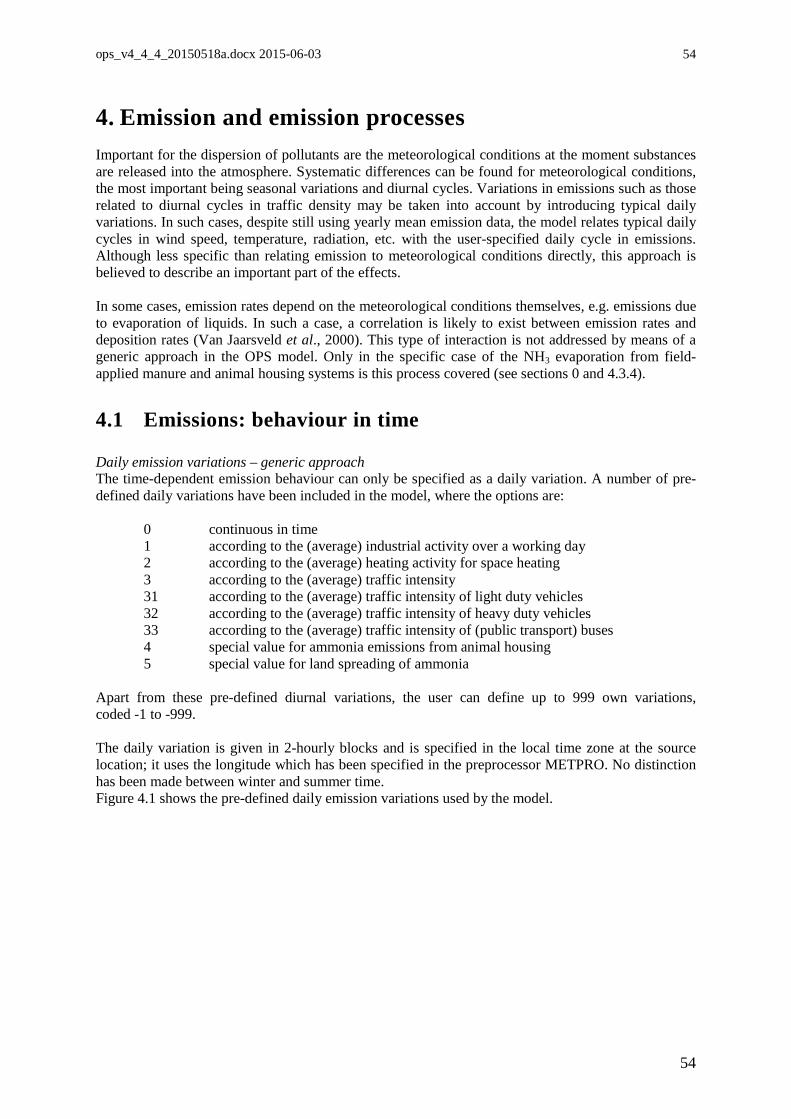
ops_v4_4_4_20150518a.docx 2015-06-03

54

4. Emission and emission processes Important for the dispersion of pollutants are the meteorological conditions at the moment substances are released into the atmosphere. Systematic differences can be found for meteorological conditions, the most important being seasonal variations and diurnal cycles. Variations in emissions such as those related to diurnal cycles in traffic density may be taken into account by introducing typical daily variations. In such cases, despite still using yearly mean emission data, the model relates typical daily cycles in wind speed, temperature, radiation, etc. with the user-specified daily cycle in emissions. Although less specific than relating emission to meteorological conditions directly, this approach is believed to describe an important part of the effects. In some cases, emission rates depend on the meteorological conditions themselves, e.g. emissions due to evaporation of liquids. In such a case, a correlation is likely to exist between emission rates and deposition rates (Van Jaarsveld et al., 2000). This type of interaction is not addressed by means of a generic approach in the OPS model. Only in the specific case of the NH3 evaporation from field-applied manure and animal housing systems is this process covered (see sections 0 and 4.3.4).

4.1 Emissions: behaviour in time Daily emission variations – generic approach The time-dependent emission behaviour can only be specified as a daily variation. A number of pre-defined daily variations have been included in the model, where the options are:

0 continuous in time 1 according to the (average) industrial activity over a working day 2 according to the (average) heating activity for space heating 3 according to the (average) traffic intensity 31 according to the (average) traffic intensity of light duty vehicles 32 according to the (average) traffic intensity of heavy duty vehicles 33 according to the (average) traffic intensity of (public transport) buses 4 special value for ammonia emissions from animal housing 5 special value for land spreading of ammonia

Apart from these pre-defined diurnal variations, the user can define up to 999 own variations, coded -1 to -999. The daily variation is given in 2-hourly blocks and is specified in the local time zone at the source location; it uses the longitude which has been specified in the preprocessor METPRO. No distinction has been made between winter and summer time. Figure 4.1 shows the pre-defined daily emission variations used by the model.

54

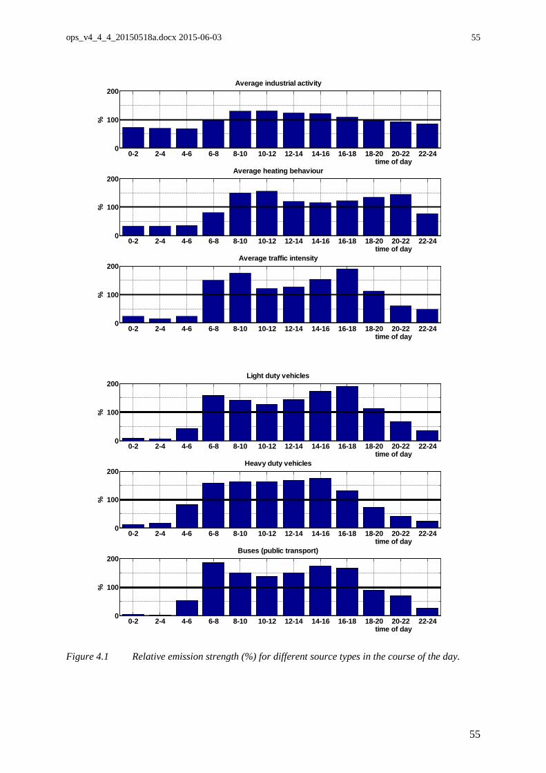
ops_v4_4_4_20150518a.docx 2015-06-03

55

0-2 2-4 4-6 6-8 8-10 10-12 12-14 14-16 16-18 18-20 20-22 22-240

100

200

time of day

%

Average industrial activity

0-2 2-4 4-6 6-8 8-10 10-12 12-14 14-16 16-18 18-20 20-22 22-240

100

200

time of day

%

Average heating behaviour

0-2 2-4 4-6 6-8 8-10 10-12 12-14 14-16 16-18 18-20 20-22 22-240

100

200

time of day

%

Average traffic intensity

0-2 2-4 4-6 6-8 8-10 10-12 12-14 14-16 16-18 18-20 20-22 22-240

100

200

time of day

%

Heavy duty vehicles

0-2 2-4 4-6 6-8 8-10 10-12 12-14 14-16 16-18 18-20 20-22 22-240

100

200

time of day

%

Buses (public transport)

0-2 2-4 4-6 6-8 8-10 10-12 12-14 14-16 16-18 18-20 20-22 22-240

100

200

time of day

%

Light duty vehicles

Figure 4.1 Relative emission strength (%) for different source types in the course of the day.

55

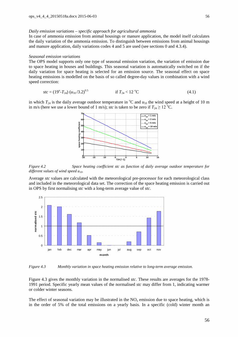
ops_v4_4_4_20150518a.docx 2015-06-03

56

Daily emission variations – specific approach for agricultural ammonia In case of ammonia emission from animal housings or manure application, the model itself calculates the daily variation of the ammonia emission. To distinguish between emissions from animal housings and manure application, daily variations codes 4 and 5 are used (see sections 0 and 4.3.4). Seasonal emission variations The OPS model supports only one type of seasonal emission variation, the variation of emission due to space heating in houses and buildings. This seasonal variation is automatically switched on if the daily variation for space heating is selected for an emission source. The seasonal effect on space heating emissions is modelled on the basis of so called degree-day values in combination with a wind speed correction:

stc = (19o-T24) (u10 /3.2)0.5 if T24 < 12 oC (4.1)

in which T24 is the daily average outdoor temperature in oC and u10 the wind speed at a height of 10 m in m/s (here we use a lower bound of 1 m/s); stc is taken to be zero if T24 ≥ 12 oC.

-20 -15 -10 -5 0 5 10 150

10

20

30

40

50

60

70

T24 [° C]

spac

e he

atin

g co

effic

ient

u10 = 1 m/su10 = 2 m/su10 = 5 m/su10 = 10 m/s

Figure 4.2 Space heating coefficient stc as function of daily average outdoor temperature for different values of wind speed u10.

Average stc values are calculated with the meteorological pre-processor for each meteorological class and included in the meteorological data set. The correction of the space heating emission is carried out in OPS by first normalising stc with a long-term average value of stc.

0

0.5

1

1.5

2

2.5

jan feb dec mar apr may jun jul aug sep oct nov

month

norm

alis

ed s

tc

Figure 4.3 Monthly variation in space heating emission relative to long-term average emission.

Figure 4.3 gives the monthly variation in the normalised stc. These results are averages for the 1978-1991 period. Specific yearly mean values of the normalised stc may differ from 1, indicating warmer or colder winter seasons. The effect of seasonal variation may be illustrated in the NOx emission due to space heating, which is in the order of 5% of the total emissions on a yearly basis. In a specific (cold) winter month an

56

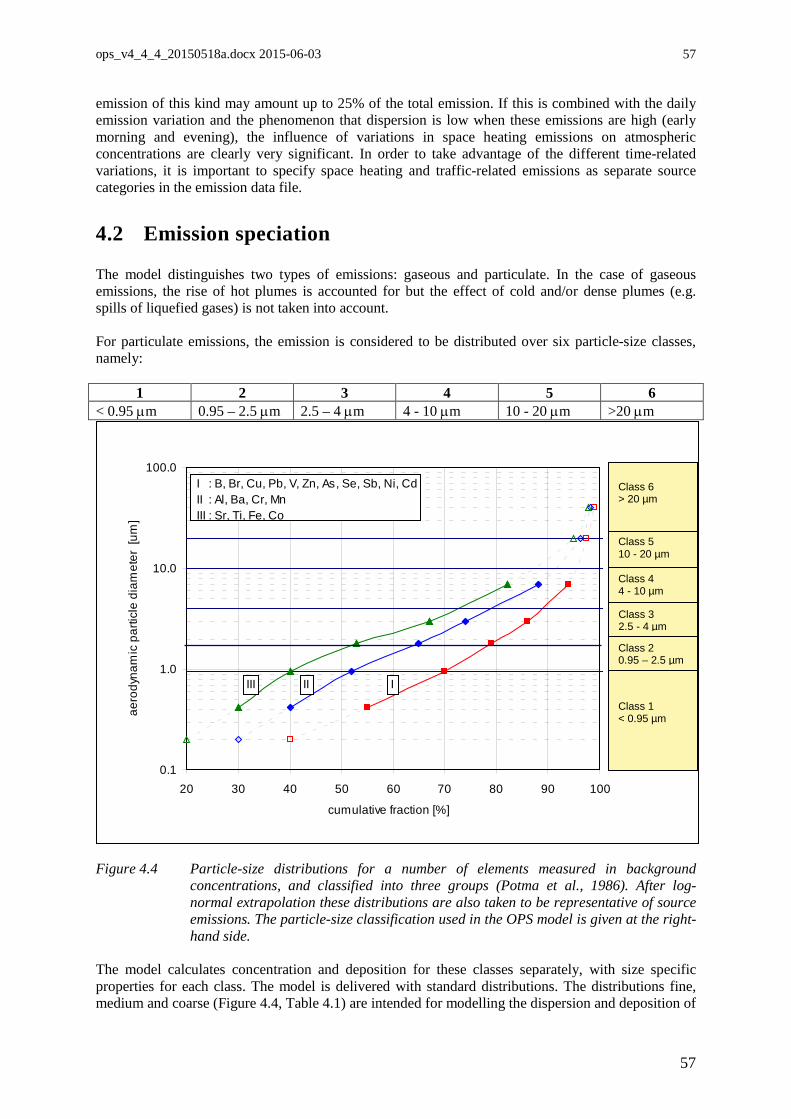
ops_v4_4_4_20150518a.docx 2015-06-03

57

emission of this kind may amount up to 25% of the total emission. If this is combined with the daily emission variation and the phenomenon that dispersion is low when these emissions are high (early morning and evening), the influence of variations in space heating emissions on atmospheric concentrations are clearly very significant. In order to take advantage of the different time-related variations, it is important to specify space heating and traffic-related emissions as separate source categories in the emission data file.

4.2 Emission speciation The model distinguishes two types of emissions: gaseous and particulate. In the case of gaseous emissions, the rise of hot plumes is accounted for but the effect of cold and/or dense plumes (e.g. spills of liquefied gases) is not taken into account. For particulate emissions, the emission is considered to be distributed over six particle-size classes, namely:

1 2 3 4 5 6 < 0.95 µm 0.95 – 2.5 µm 2.5 – 4 µm 4 - 10 µm 10 - 20 µm >20 µm

Figure 4.4 Particle-size distributions for a number of elements measured in background

concentrations, and classified into three groups (Potma et al., 1986). After log-normal extrapolation these distributions are also taken to be representative of source emissions. The particle-size classification used in the OPS model is given at the right-hand side.

The model calculates concentration and deposition for these classes separately, with size specific properties for each class. The model is delivered with standard distributions. The distributions fine, medium and coarse (Figure 4.4, Table 4.1) are intended for modelling the dispersion and deposition of

0.1

1.0

10.0

100.0

20 30 40 50 60 70 80 90 100

cumulative fraction [%]

aero

dyna

mic

par

ticle

dia

met

er [

um]

Class 5 > 20 um

Class 1 < 0.95 um

Class 410 - 20 um

Class 20.95 - 4 um

Class 3 4 - 10 um

IIIIII

I : B, Br, Cu, Pb, V, Zn, As, Se, Sb, Ni, Cd II : Al, Ba, Cr, Mn III : Sr, Ti, Fe, Co

Class 1 < 0.95 µm

Class 2 0.95 – 2.5 µm

Class 3 2.5 - 4 µm

Class 4 4 - 10 µm

Class 5 10 - 20 µm

Class 6 > 20 µm

57

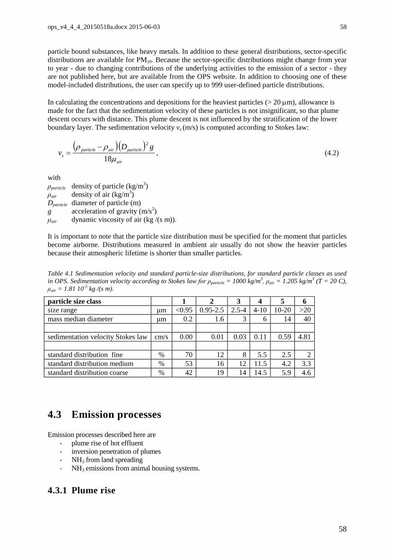
ops_v4_4_4_20150518a.docx 2015-06-03

58

particle bound substances, like heavy metals. In addition to these general distributions, sector-specific distributions are available for PM10. Because the sector-specific distributions might change from year to year - due to changing contributions of the underlying activities to the emission of a sector - they are not published here, but are available from the OPS website. In addition to choosing one of these model-included distributions, the user can specify up to 999 user-defined particle distributions. In calculating the concentrations and depositions for the heaviest particles (> 20 µm), allowance is made for the fact that the sedimentation velocity of these particles is not insignificant, so that plume descent occurs with distance. This plume descent is not influenced by the stratification of the lower boundary layer. The sedimentation velocity vs (m/s) is computed according to Stokes law:

( ) ( )

air

particleairparticles

gDv

µρρ18

2−= , (4.2)

with ρparticle density of particle (kg/m3) ρair density of air (kg/m3) Dparticle diameter of particle (m) g acceleration of gravity (m/s2) μair dynamic viscosity of air (kg /(s m)). It is important to note that the particle size distribution must be specified for the moment that particles become airborne. Distributions measured in ambient air usually do not show the heavier particles because their atmospheric lifetime is shorter than smaller particles. Table 4.1 Sedimentation velocity and standard particle-size distributions, for standard particle classes as used in OPS. Sedimentation velocity according to Stokes law for ρparticle = 1000 kg/m3, ρair = 1.205 kg/m3 (T = 20 C), μair = 1.81 10-5 kg /(s m).

particle size class 1 2 3 4 5 6 size range μm <0.95 0.95-2.5 2.5-4 4-10 10-20 >20 mass median diameter μm 0.2 1.6 3 6 14 40 sedimentation velocity Stokes law cm/s 0.00 0.01 0.03 0.11 0.59 4.81 standard distribution fine % 70 12 8 5.5 2.5 2 standard distribution medium % 53 16 12 11.5 4.2 3.3 standard distribution coarse % 42 19 14 14.5 5.9 4.6

4.3 Emission processes Emission processes described here are

- plume rise of hot effluent - inversion penetration of plumes - NH3 from land spreading - NH3 emissions from animal housing systems.

4.3.1 Plume rise

58

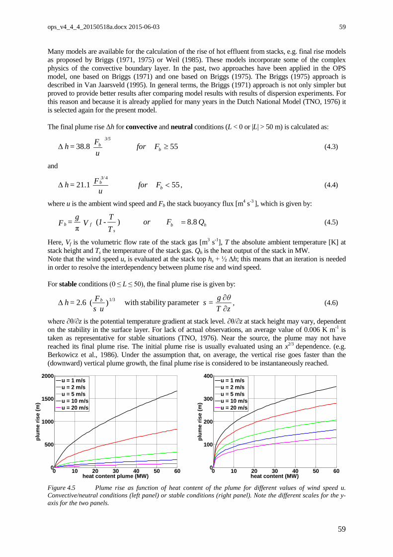
ops_v4_4_4_20150518a.docx 2015-06-03

59

Many models are available for the calculation of the rise of hot effluent from stacks, e.g. final rise models as proposed by Briggs (1971, 1975) or Weil (1985). These models incorporate some of the complex physics of the convective boundary layer. In the past, two approaches have been applied in the OPS model, one based on Briggs (1971) and one based on Briggs (1975). The Briggs (1975) approach is described in Van Jaarsveld (1995). In general terms, the Briggs (1971) approach is not only simpler but proved to provide better results after comparing model results with results of dispersion experiments. For this reason and because it is already applied for many years in the Dutch National Model (TNO, 1976) it is selected again for the present model. The final plume rise Δh for convective and neutral conditions (L < 0 or |L| > 50 m) is calculated as:

558.83 ≥∆ bb

3/5

FforuF = h (4.3)

and

551.214

<∆ b

3/ b Ffor u

F = h , (4.4)

where u is the ambient wind speed and Fb the stack buoyancy flux [m4 s-3 ], which is given by:

hbs

fb QFor TT - 1 V g = F 8.8)(

π= (4.5)

Here, Vf is the volumetric flow rate of the stack gas [m3 s-1], T the absolute ambient temperature [K] at stack height and Ts the temperature of the stack gas. Qh is the heat output of the stack in MW. Note that the wind speed u, is evaluated at the stack top hs + ½ Δh; this means that an iteration is needed in order to resolve the interdependency between plume rise and wind speed. For stable conditions (0 ≤ L ≤ 50), the final plume rise is given by:

zθ

Tgs =

u sF = h b

∂∂

∆ parameterstability with )( 2.6 1/3 , (4.6)

where ∂θ/∂z is the potential temperature gradient at stack level. ∂θ/∂z at stack height may vary, dependent on the stability in the surface layer. For lack of actual observations, an average value of 0.006 K m-1 is taken as representative for stable situations (TNO, 1976). Near the source, the plume may not have reached its final plume rise. The initial plume rise is usually evaluated using an x2/3 dependence. (e.g. Berkowicz et al., 1986). Under the assumption that, on average, the vertical rise goes faster than the (downward) vertical plume growth, the final plume rise is considered to be instantaneously reached.

0 10 20 30 40 50 600

500

1000

1500

2000

heat content plume (MW)

plum

e ris

e (m

)

u = 1 m/su = 2 m/su = 5 m/su = 10 m/su = 20 m/s

0 10 20 30 40 50 600

100

200

300

400

heat content (MW)

plum

e ris

e (m

)

u = 1 m/su = 2 m/su = 5 m/su = 10 m/su = 20 m/s

Figure 4.5 Plume rise as function of heat content of the plume for different values of wind speed u. Convective/neutral conditions (left panel) or stable conditions (right panel). Note the different scales for the y-axis for the two panels.

59

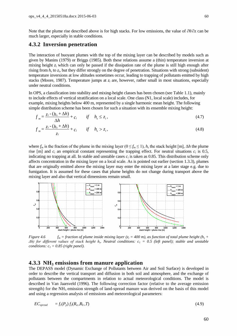
ops_v4_4_4_20150518a.docx 2015-06-03

60

Note that the plume rise described above is for high stacks. For low emissions, the value of ∂θ/∂z can be much larger, especially in stable conditions.

4.3.2 Inversion penetration The interaction of buoyant plumes with the top of the mixing layer can be described by models such as given by Manins (1979) or Briggs (1985). Both these relations assume a (thin) temperature inversion at mixing height zi which can only be passed if the dissipation rate of the plume is still high enough after rising from hs to zi, but they differ strongly on the degree of penetration. Situations with strong (subsident) temperature inversions at low altitudes sometimes occur, leading to trapping of pollutants emitted by high stacks (Moore, 1987). Temperature jumps at zi are, however, rather small in most situations, especially under neutral conditions.

In OPS, a classification into stability and mixing-height classes has been chosen (see Table 1.1), mainly to include effects of vertical stratification on a local scale. One class (N1, local scale) includes, for example, mixing heights below 400 m, represented by a single harmonic mean height. The following simple distribution scheme has been chosen for such a situation with its ensemble mixing height:

isisi

m zhif c + h

h+ h - z = f ≤∆

∆ )(, (4.7)

isii

sim zhif c +

zh+ h - z = f >

∆ )(, (4.8)

where fm is the fraction of the plume in the mixing layer (0 ≤ fm ≤ 1), hs the stack height [m], Δh the plume rise [m] and ci an empirical constant representing the trapping effect. For neutral situations ci is 0.5, indicating no trapping at all. In stable and unstable cases ci is taken as 0.85. This distribution scheme only affects concentration in the mixing layer on a local scale. As is pointed out earlier (section 1.3.3), plumes that are originally emitted above the mixing layer may enter the mixing layer at a later stage e.g. due to fumigation. It is assumed for these cases that plume heights do not change during transport above the mixing layer and also that vertical dimensions remain small.

0 200 400 600 800 1000 1200 14000

0.2

0.4

0.6

0.8

1

stack height + plume rise (m)

f m

hstack = 1 mhstack = 100 mhstack = 200 m

0 200 400 600 800 1000 1200 14000

0.2

0.4

0.6

0.8

1

stack height + plume rise (m)

f m

hstack = 1 mhstack = 100 mhstack = 200 m

Figure 4.6 fm = fraction of plume inside mixing layer (zi = 400 m), as function of total plume height (hs + Δh) for different values of stack height hs. Neutral conditions: c1 = 0.5 (left panel); stable and unstable conditions: c1 = 0.85 (right panel).

4.3.3 NH3 emissions from manure application The DEPASS model (Dynamic Exchange of Pollutants between Air and Soil Surface) is developed in order to describe the vertical transport and diffusion in both soil and atmosphere, and the exchange of pollutants between the compartments in relation to actual meteorological conditions. The model is described in Van Jaarsveld (1996). The following correction factor (relative to the average emission strength) for the NH3 emission strength of land-spread manure was derived on the basis of this model and using a regression analysis of emissions and meteorological parameters: ECspread = f1(Pp) f2(Ra ,Rb ,T) (4.9)

60

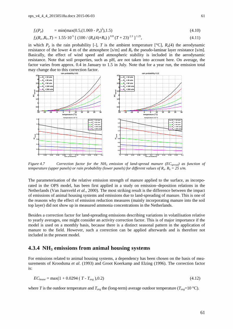
ops_v4_4_4_20150518a.docx 2015-06-03

61

f1(Pp) = min(max(0.5,(1.069 - Pp)2),1.5) (4.10)

f2(Ra ,Rb ,T) = 1.55·10-5 [ (100 / (Ra(4)+Rb) ) 0.8 (T + 23) 2.3 ] 1.25, (4.11)

in which Pp is the rain probability [-], T is the ambient temperature [°C], Ra(4) the aerodynamic resistance of the lower 4 m of the atmosphere [s/m] and Rb the pseudo-laminar layer resistance [s/m]. Basically, the effect of wind speed and atmospheric stability is included in the aerodynamic resistance. Note that soil properties, such as pH, are not taken into account here. On average, the factor varies from approx. 0.4 in January to 1.5 in July. Note that for a year run, the emission total may change due to this correction factor.

-20 -15 -10 -5 0 5 10 15 20 25 300

0.5

1

1.5

2

2.5

3

3.5

4

4.5rain probability 0.03

temperature (oC)

ECsp

read

Ra = 10 s/mRa = 20 s/mRa = 50 s/mRa = 100 s/mRa = 200 s/m

-20 -15 -10 -5 0 5 10 15 20 25 300

0.5

1

1.5

2

2.5

3

3.5

4

4.5rain probability 0.12

temperature (oC)EC

spre

ad

Ra = 10 s/mRa = 20 s/mRa = 50 s/mRa = 100 s/mRa = 200 s/m

0 0.02 0.04 0.06 0.08 0.1 0.12 0.14 0.16 0.18 0.20

0.2

0.4

0.6

0.8

1

1.2

1.4temperature 10 oC

rain probability

ECsp

read

Ra = 10 s/mRa = 20 s/mRa = 50 s/mRa = 100 s/mRa = 200 s/m

0 0.02 0.04 0.06 0.08 0.1 0.12 0.14 0.16 0.18 0.20

0.2

0.4

0.6

0.8

1

1.2

1.4

1.6

1.8temperature 15 oC

rain probability

ECsp

read

Ra = 10 s/mRa = 20 s/mRa = 50 s/mRa = 100 s/mRa = 200 s/m

Figure 4.7 Correction factor for the NH3 emission of land-spread manure (ECspread) as function of temperature (upper panels) or rain probability (lower panels) for different values of Ra. Rb = 25 s/m.

The parameterisation of the relative emission strength of manure applied to the surface, as incorpo-rated in the OPS model, has been first applied in a study on emission−deposition relations in the Netherlands (Van Jaarsveld et al., 2000). The most striking result is the difference between the impact of emissions of animal housing systems and emissions due to land-spreading of manure. This is one of the reasons why the effect of emission reduction measures (mainly incorporating manure into the soil top layer) did not show up in measured ammonia concentrations in the Netherlands. Besides a correction factor for land-spreading emissions describing variations in volatilisation relative to yearly averages, one might consider an activity correction factor. This is of major importance if the model is used on a monthly basis, because there is a distinct seasonal pattern in the application of manure to the field. However, such a correction can be applied afterwards and is therefore not included in the present model.

4.3.4 NH3 emissions from animal housing systems For emissions related to animal housing systems, a dependency has been chosen on the basis of mea-surements of Kroodsma et al. (1993) and Groot Koerkamp and Elzing (1996). The correction factor is: EChouse = max(1 + 0.0294 ( T - Tavg ),0.2) (4.12) where T is the outdoor temperature and Tavg the (long-term) average outdoor temperature (Tavg=10 °C).

61

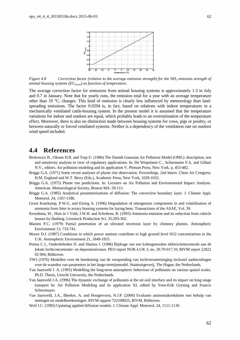
ops_v4_4_4_20150518a.docx 2015-06-03

62

-20 -15 -10 -5 0 5 10 15 20 25 300

0.2

0.4

0.6

0.8

1

1.2

1.4

1.6

temperature (oC)

ECho

use

Figure 4.8 Correction factor (relative to the average emission strength) for the NH3 emission strength of animal housing systems (EChouse) as function of temperature.

The average correction factor for emissions from animal housing systems is approximately 1.3 in July and 0.7 in January. Note that for yearly runs, the emission total for a year with an average temperature other than 10 °C, changes. This kind of emission is clearly less influenced by meteorology than land-spreading emissions. The factor 0.0294 is, in fact, based on relations with indoor temperatures in a mechanically ventilated cattle-housing system. In the present model it is assumed that the temperature variations for indoor and outdoor are equal, which probably leads to an overestimation of the temperature effect. Moreover, there is also no distinction made between housing systems for cows, pigs or poultry, or between naturally or forced ventilated systems. Neither is a dependency of the ventilation rate on outdoor wind speed included.

4.4 References Berkowicz R., Olesen H.R. and Torp U. (1986) The Danish Gaussian Air Pollution Model (OML): description, test

and sensitivity analysis in view of regulatory applications. In: De Wispelaere C., Schiermeier F.A. and Gillani N.V., editors. Air pollution modeling and its application V. Plenum Press, New York. p. 453-482.

Briggs G.A. (1971) Some recent analyses of plume rise observation. Proceedings. 2nd Intern. Clean Air Congress, H.M. Englund and W.T. Berry (Eds.), Academic Press, New York, 1029-1032.

Briggs G.A. (1975) Plume rise predictions. In: Lectures on Air Pollution and Environmental Impact Analysis. American. Meteorological Society, Boston MA. 59-111.

Briggs G.A. (1985) Analytical parameterisations of diffusion: The convective boundary layer. J. Climate Appl. Meteorol. 24, 1167-1186.

Groot Koerkamp, P.W.G. and Elzing A. (1996) Degradation of nitrogenous components in and volatilization of ammonia from litter in aviary housing systems for laying hens. Transactions of the ASAE, Vol. 39.

Kroodsma, W., Huis in 't Veld, J.W.H. and Scholtens, R. (1993) Ammonia emission and its reduction from cubicle houses by flushing. Livestock Production Sci. 35:293-302.

Manins P.C. (1979) Partial penetration of an elevated inversion layer by chimney plumes. Atmospheric Environment 13, 733-741.

Moore D.J. (1987) Conditions in which power stations contribute to high ground level SO2 concentrations in the U.K. Atmospheric Environment 21, 1849-1855.

Potma C.J., Onderdelinden D. and Slanina J. (1986) Bijdrage van een kolengestookte elektriciteitscentrale aan de lokale luchtconcentratie- en depositieniveaus. PEO report NOK-LUK 3, no. 20.70-017.10, RIVM report 22822 02 004, Bilthoven.

TNO (1976) Modellen voor de berekening van de verspreiding van luchtverontreiniging inclusief aanbevelingen voor de waarden van parameters in het lange-termijnmodel. Staatsuitgeverij, The Hague, the Netherlands.

Van Jaarsveld J. A. (1995) Modelling the long-term atmospheric behaviour of pollutants on various spatial scales. Ph.D. Thesis, Utrecht University, the Netherlands.

Van Jaarsveld J.A. (1996) The dynamic exchange of pollutants at the air-soil interface and its impact on long range transport In: Air Pollution Modeling and its application XI, edited by Sven-Erik Gryning and Francis Schiermayer.

Van Jaarsveld, J.A., Bleeker, A. and Hoogervorst, N.J.P. (2000) Evaluatie ammoniakredukties met behulp van metingen en modelberekeningen. RIVM rapport 722108025, RIVM, Bilthoven.

Weil J.C. (1985) Updating applied diffusion models. J. Climate Appl. Meteorol. 24, 1111-1130.

62

ops_v4_4_4_20150518a.docx, 2015-06-03 63

5. Dry deposition Deposition flux and deposition velocity The vertical transport of atmospheric contaminants - either in gaseous or in particle form - to or from the underlying surface is governed by a number of processes. Some of these are determined by atmospheric properties common to all contaminants and others by specific physical and chemical properties of the gases in conjunction with properties of the surface. The vertical exchange flux Fd in this model is described as the product of a vertical velocity vd specified for a height z, and the difference in concentration at this height, χa, and the surface or substrate concentration χs:

][ - (z) (z) v = F sadd χχ . (5.1)

For substances which immediately react at the surface with other substances or for substances attached to particles, χs may be considered zero. However, for substances such as ammonia or persistent organic pollutants (POPs), χs may be so high under specific conditions that the vertical flux is upward (Van Jaarsveld et al., 1994). In that case Eq. (5.1) describes the emission flux. For gases such as nitrogen oxide (NO) this may be the case for most ecosystems (Duyzer and Fowler, 1994). In an electrical analogue vd(z) can be represented as a contaminant conductivity, which can be expressed as the inverse of resistances:

])([)( -1 R + R + zR = zv cbad . (5.2)

The sequence of the three resistances represents the resistances in the three stages of vertical transport, i.e. (1) for the turbulent layer, the aerodynamic resistance Ra, (2) for the layer immediately adjacent to the surface, the pseudo-laminar layer resistance Rb, and (3) for the receptor the surface resistance Rc. Note that OPS computes deposition at two different locations: - along the transport trajectory (using parameters averaged along the trajectory); see section 5.1; - at the receptor (using local parameters at the receptor's site). Aerodynamic resistance Ra The resistance Ra depends mainly on the local atmospheric turbulence. Hicks et al. (1989) assume that the atmospheric resistance to transport of gases and small particles is similar to that of heat. Here Wesely and Hicks (1977) are followed; they approximate Ra by:

] )()()(ln[1)(*

Lz +

Lz -

zz

u = z R 0

hh0

a ψψκ

, (5.3)

where ψh(z/L) is the stability correction for heat, which is related to the dimensionless temperature gradient φh (see Eq. (3.22) and (3.23):

( ) ζζ

ζϕψ d =

Lz L

zh

h ∫

−

0

1 , (5.4)

which can be approximated by (Beljaars and Holtslag, 1990):

−+

Lz =

Lz h 16115.0log2)(ψ for L ≤ 0, (5.5)

72.1035.0exp72.1075.00.7- =)( −

−

−−

Lz

Lz

Lz

Lz hψ for L > 0. (5.6)

Strictly speaking, the aerodynamic resistance is the resistance between height z and the zero plane displacement d [m], however, in OPS, d is set to zero.

63

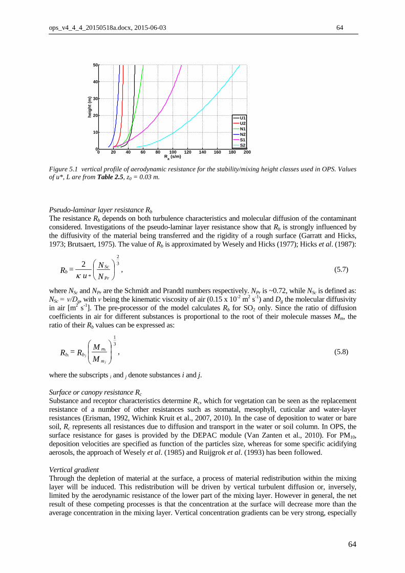
ops_v4_4_4_20150518a.docx, 2015-06-03 64

0 20 40 60 80 100 120 140 160 180 2000

10

20

30

40

50

Ra (s/m)

heig

ht (m

)

U1U2N1N2S1S2

Figure 5.1 vertical profile of aerodynamic resistance for the stability/mixing height classes used in OPS. Values of u*, L are from Table 2.5, z0 = 0.03 m.

Pseudo-laminar layer resistance Rb The resistance Rb depends on both turbulence characteristics and molecular diffusion of the contaminant considered. Investigations of the pseudo-laminar layer resistance show that Rb is strongly influenced by the diffusivity of the material being transferred and the rigidity of a rough surface (Garratt and Hicks, 1973; Brutsaert, 1975). The value of Rb is approximated by Wesely and Hicks (1977); Hicks et al. (1987):

NN

u = R

Pr

Sc

b

32

*

2κ

, (5.7)

where NSc and NPr are the Schmidt and Prandtl numbers respectively. NPr is ~0.72, while NSc is defined as: NSc = ν/Dg, with ν being the kinematic viscosity of air (0.15 x 10-2 m2 s-1) and Dg the molecular diffusivity in air [m2 s-1]. The pre-processor of the model calculates Rb for SO2 only. Since the ratio of diffusion coefficients in air for different substances is proportional to the root of their molecule masses Mm, the ratio of their Rb values can be expressed as:

MM R = R

m

m

bbj

iji

31

, (5.8)

where the subscripts i and j denote substances i and j. Surface or canopy resistance Rc Substance and receptor characteristics determine Rc, which for vegetation can be seen as the replacement resistance of a number of other resistances such as stomatal, mesophyll, cuticular and water-layer resistances (Erisman, 1992, Wichink Kruit et al., 2007, 2010). In the case of deposition to water or bare soil, Rc represents all resistances due to diffusion and transport in the water or soil column. In OPS, the surface resistance for gases is provided by the DEPAC module (Van Zanten et al., 2010). For PM10, deposition velocities are specified as function of the particles size, whereas for some specific acidifying aerosols, the approach of Wesely et al. (1985) and Ruijgrok et al. (1993) has been followed. Vertical gradient Through the depletion of material at the surface, a process of material redistribution within the mixing layer will be induced. This redistribution will be driven by vertical turbulent diffusion or, inversely, limited by the aerodynamic resistance of the lower part of the mixing layer. However in general, the net result of these competing processes is that the concentration at the surface will decrease more than the average concentration in the mixing layer. Vertical concentration gradients can be very strong, especially

64

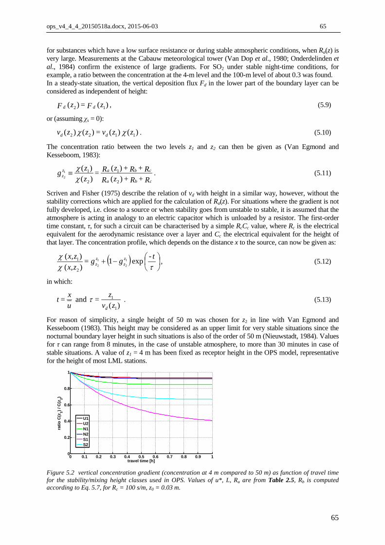
ops_v4_4_4_20150518a.docx, 2015-06-03 65

for substances which have a low surface resistance or during stable atmospheric conditions, when Ra(z) is very large. Measurements at the Cabauw meteorological tower (Van Dop et al., 1980; Onderdelinden et al., 1984) confirm the existence of large gradients. For SO2 under stable night-time conditions, for example, a ratio between the concentration at the 4-m level and the 100-m level of about 0.3 was found. In a steady-state situation, the vertical deposition flux Fd in the lower part of the boundary layer can be considered as independent of height:

)()( 12 z F = z F dd , (5.9)

or (assuming χs = 0):

)()()()( 1122 z zv =zzv dd χχ . (5.10)

The concentration ratio between the two levels z1 and z2 can then be given as (Van Egmond and Kesseboom, 1983):

R + R + z RR + R + z R =

zzg

cba

cbazz )(

)()()(

2

1

2

11

2 χχ

≡ . (5.11)

Scriven and Fisher (1975) describe the relation of vd with height in a similar way, however, without the stability corrections which are applied for the calculation of Ra(z). For situations where the gradient is not fully developed, i.e. close to a source or when stability goes from unstable to stable, it is assumed that the atmosphere is acting in analogy to an electric capacitor which is unloaded by a resistor. The first-order time constant, τ, for such a circuit can be characterised by a simple RcCc value, where Rc is the electrical equivalent for the aerodynamic resistance over a layer and Cc the electrical equivalent for the height of that layer. The concentration profile, which depends on the distance x to the source, can now be given as:

( )

−+τχ

χ t- g g = zx, zx, z

zzz exp1

)()(

1

2

1

22

1 , (5.12)

in which:

)(

= and1

1

zvz

ux = t

d

τ . (5.13)

For reason of simplicity, a single height of 50 m was chosen for z2 in line with Van Egmond and Kesseboom (1983). This height may be considered as an upper limit for very stable situations since the nocturnal boundary layer height in such situations is also of the order of 50 m (Nieuwstadt, 1984). Values for τ can range from 8 minutes, in the case of unstable atmosphere, to more than 30 minutes in case of stable situations. A value of z1 = 4 m has been fixed as receptor height in the OPS model, representative for the height of most LML stations.

0 0.1 0.2 0.3 0.4 0.5 0.6 0.7 0.8 0.9 10

0.2

0.4

0.6

0.8

1

travel time [h]

ratio

C(z

1) / C

(z2)

U1U2N1N2S1S2

Figure 5.2 vertical concentration gradient (concentration at 4 m compared to 50 m) as function of travel time for the stability/mixing height classes used in OPS. Values of u*, L, Ra are from Table 2.5, Rb is computed according to Eq. 5.7, for Rc = 100 s/m, z0 = 0.03 m.

65

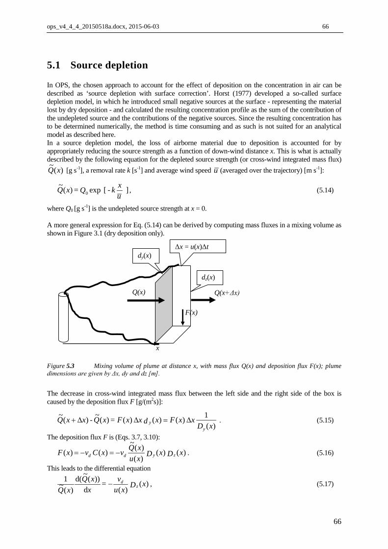
ops_v4_4_4_20150518a.docx, 2015-06-03 66

5.1 Source depletion In OPS, the chosen approach to account for the effect of deposition on the concentration in air can be described as ‘source depletion with surface correction’. Horst (1977) developed a so-called surface depletion model, in which he introduced small negative sources at the surface - representing the material lost by dry deposition - and calculated the resulting concentration profile as the sum of the contribution of the undepleted source and the contributions of the negative sources. Since the resulting concentration has to be determined numerically, the method is time consuming and as such is not suited for an analytical model as described here. In a source depletion model, the loss of airborne material due to deposition is accounted for by appropriately reducing the source strength as a function of down-wind distance x. This is what is actually described by the following equation for the depleted source strength (or cross-wind integrated mass flux)

xQ )(~[g s-1], a removal rate k [s-1] and average wind speed u (averaged over the trajectory) [m s-1]:

][exp)(~0

uxk- Q = xQ , (5.14)

where Q0 [g s-1] is the undepleted source strength at x = 0. A more general expression for Eq. (5.14) can be derived by computing mass fluxes in a mixing volume as shown in Figure 3.1 (dry deposition only).

Figure 5.3 Mixing volume of plume at distance x, with mass flux Q(x) and deposition flux F(x); plume dimensions are given by Δx, dy and dz [m].

The decrease in cross-wind integrated mass flux between the left side and the right side of the box is caused by the deposition flux F [g/(m2s)]:

)(

1)()()()(~-)(~xD

x xFxd x xF= xQxxQy

y ∆=∆∆+ . (5.15)

The deposition flux F is (Eqs. 3.7, 3.10):

)()()()(~

)()( xD xD xuxQvxCv xF zydd −=−= . (5.16)

This leads to the differential equation

)()(d

))(~d()(~

1 xD xuv=

xxQ

xQ zd− , (5.17)

x

Q(x)

Δx = u(x)Δt

dz(x)

dy(x)

F(x)

Q(x+Δx)

66

ops_v4_4_4_20150518a.docx, 2015-06-03 67

with solution

])([exp)(~

00 d D u

v - Q = xQ zd

x

xx∫ . (5.18)

As pointed out earlier, the expression Dz(x) depends on the ratio σz /zi, (zi mixing height [m]), resulting in either Eq. (3.9) or (3.15). In addition, the effective transport height has a tendency to increase with distance, also resulting in an increasing transport velocity ū. Therefore, the integral in Eq. (5.18) cannot be solved analytically for the entire range of x, but has to be split in two or more parts, representing the different stages in plume development from source to receptor. For this reason three stages are distinguished: I. Transport within an area source with radius ra. The vertical dispersion within such a source is

characterised by σz,eff (x) (Eq. (3.42)). This effective vertical dispersion parameter is almost independent of the position within the area source (see Figure 3.12). Therefore Dz(x) is approached by:

)(2π

2)(aeffz

z r = x = xD

σ. (5.19)

and the depleted source strength is

])(2

2)([exp)(~0

rxux z v- Q = xQ

aeffz

dd

=σp, (5.20)

in which u is the transport velocity taken at z = σz,eff (x). The effective distance xd over which deposition takes place within an area source is (assuming that, on average, the receptor lies halfway between the centre and the edge of the area source):

( )ktrx ad −

= exp

2, (5.21)

with k [s-1] the total conversion rate for chemical conversion, wet deposition and dry deposition and t [s] the travel time from area source to receptor: t = (ra /2)/u.

II. The phase where the plume is not yet uniformly mixed in the mixing layer. This stage starts at xs

= 0 in case of a point source or at xs = ra in the case of an area source. A separate description of this phase is especially important for low-level sources because of the enhanced ground-level concentrations close to the source. Dz(x) is given by Eq. (3.15). When the reflection against the top of the mixing layer is neglected at this point (Eq. (3.15) is dominated by the last term anyway), Dz(x) can be written as:

h-

= x Dzz

z

2

2

2exp

2π2)(

σσ. (5.22)

An approximation for the solution of Eq. (5.18) in combination with (5.22) is based on the assumption that u / x K zz 22 =σ (see 3.24), with a the turbulent eddy diffusivity Kz [m2/s], that does not depend on the distance x. In appendix 5.5.1, the following expression is derived for the source depletion ratio between xs and x:

67

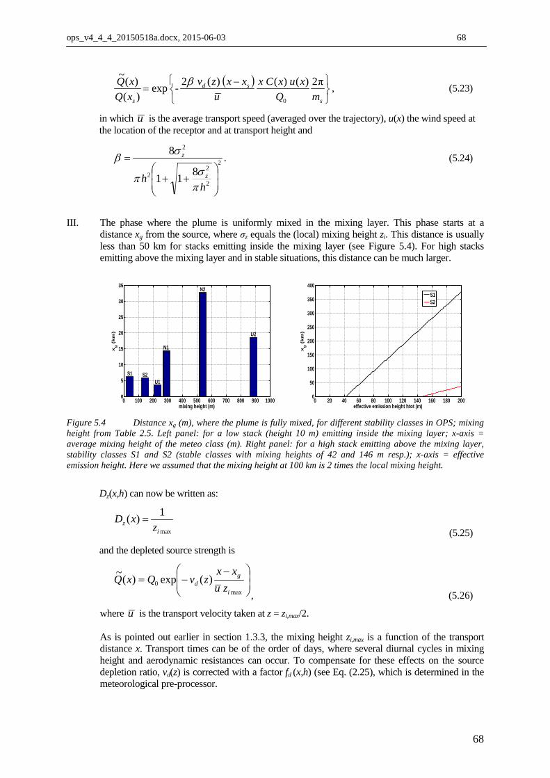
ops_v4_4_4_20150518a.docx, 2015-06-03 68

( )

−

=s

sd

s mQxuxCx

uxxzv-

xQxQ π2)()()(2exp

)()(~

0

β , (5.23)

in which u is the average transport speed (averaged over the trajectory), u(x) the wind speed at the location of the receptor and at transport height and

.811

82

2

22

2

++

=

hh z

z

pσp

σβ (5.24)

III. The phase where the plume is uniformly mixed in the mixing layer. This phase starts at a distance xg from the source, where σz equals the (local) mixing height zi. This distance is usually less than 50 km for stacks emitting inside the mixing layer (see Figure 5.4). For high stacks emitting above the mixing layer and in stable situations, this distance can be much larger.

0 100 200 300 400 500 600 700 800 900 10000

5

10

15

20

25

30

35

U1

U2

N1

N2

S1 S2

mixing height (m)

xg (

km

)

0 20 40 60 80 100 120 140 160 180 2000

50

100

150

200

250

300

350

400

effective emission height htot (m)

xg (

km

)

S1S2

Figure 5.4 Distance xg (m), where the plume is fully mixed, for different stability classes in OPS; mixing height from Table 2.5. Left panel: for a low stack (height 10 m) emitting inside the mixing layer; x-axis = average mixing height of the meteo class (m). Right panel: for a high stack emitting above the mixing layer, stability classes S1 and S2 (stable classes with mixing heights of 42 and 146 m resp.); x-axis = effective emission height. Here we assumed that the mixing height at 100 km is 2 times the local mixing height.

Dz(x,h) can now be written as:

max

1)(i

z zxD =

(5.25)

and the depleted source strength is

−−=

max0 )(exp)(~

i

gd zu

xxzvQxQ

, (5.26)

where u is the transport velocity taken at z = zi,max/2. As is pointed out earlier in section 1.3.3, the mixing height zi,max is a function of the transport distance x. Transport times can be of the order of days, where several diurnal cycles in mixing height and aerodynamic resistances can occur. To compensate for these effects on the source depletion ratio, vd(z) is corrected with a factor fd (x,h) (see Eq. (2.25), which is determined in the meteorological pre-processor.

68

ops_v4_4_4_20150518a.docx, 2015-06-03 69

For the three phases of the plume, various transport velocities are applied, depending on the height of the centre of the plume mass. Also the height for which vd is specified depends on the phase of the plume. In principle, vd has to be specified for the lowest height where the vertical concentration distribution is not yet disturbed by the dry deposition process. In phase I (inside area source), vd is taken at z = 4 m. For phase II (Gaussian plume, no gradient due to deposition), vd is taken at z = 0 m, while for phase III (well-mixed) vd is taken at z = 50 m. The vertical profile correction (Eq. 5.12) is started at the beginning of phase II, but has most of its effects in phase III. The source depletion ratio at a (large) distance from an area source, due to dry deposition, is calculated as the product of the depletion ratios in the different stages of plume development.

5.2 Source depletion for heavy plumes In appendix 0, (Onderdelinden, 1985) derives the following expressions for the source depletion ratio's of heavy plumes:

( ) hpppp

p-

Q

xQ≥

+++

++≈ δ,

π4

1

π4

1expπ1)(~

222

211

21

(5.27)

( ) ,,

π4

1

π4

1expπ11)(~

222

211

21 h

ppppp-

QxQ

<

++−

++−−≈ δ (5.28)

with

z

h-pσδ

21+

= , z

hpσδ

22+

= , Q source strength [g/s], Q~ depleted source strength [g/s], σz vertical

dispersion length [m], h emission height [m], δ plume descent [m]:

uxvs=δ , (5.29)

where vs : settling velocity of heavy particles [m/s], x: down-wind distance from source [m], u: wind speed [m/s]. Onderdelinden (1985) showed that the deposition velocity for heavy plumes is half the settling velocity (see also appendix 0).

69

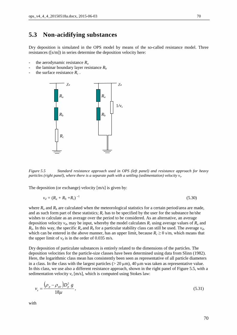
ops_v4_4_4_20150518a.docx, 2015-06-03 70

5.3 Non-acidifying substances Dry deposition is simulated in the OPS model by means of the so-called resistance model. Three resistances ([s/m]) in series determine the deposition velocity here: - the aerodynamic resistance Ra

- the laminar boundary layer resistance Rb - the surface resistance Rc .

Figure 5.5 Standard resistance approach used in OPS (left panel) and resistance approach for heavy particles (right panel), where there is a separate path with a settling (sedimentation) velocity vs.

The deposition (or exchange) velocity [m/s] is given by:

vd = (Ra + Rb +Rc) –1 (5.30) where Ra and Rb are calculated when the meteorological statistics for a certain period/area are made, and as such form part of these statistics; Rc has to be specified by the user for the substance he/she wishes to calculate as an average over the period to be considered. As an alternative, an average deposition velocity vd, may be input, whereby the model calculates Rc using average values of Ra and Rb. In this way, the specific Ra and Rb for a particular stability class can still be used. The average vd, which can be entered in the above manner, has an upper limit, because Rc ≥ 0 s/m, which means that the upper limit of vd is in the order of 0.035 m/s. Dry deposition of particulate substances is entirely related to the dimensions of the particles. The deposition velocities for the particle-size classes have been determined using data from Slinn (1982). Here, the logarithmic class mean has consistently been seen as representative of all particle diameters in a class. In the class with the largest particles (> 20 µm), 40 µm was taken as representative value. In this class, we use also a different resistance approach, shown in the right panel of Figure 5.5, with a sedimentation velocity vs [m/s], which is computed using Stokes law:

( )

µρρ18

2 gDv pairp

s

−= , (5.31)

with

Ra

Rb

1/vs

Ra

Rb

Rc

χa χa

70

ops_v4_4_4_20150518a.docx, 2015-06-03 71

vs : sedimentation or terminal settling velocity [m/s] ρp : density of particle ~ 1000 kg/m3 ρair : density of air = 1.293 kg/m3 (0 °C), 1.205 kg/m3 (20 °C) Dp : diameter of particle [m] g : acceleration of gravity = 9.807 m/s2 μ : viscosity of air = 1.81·10-5 kg /(s m). The effective deposition velocity is only influenced by the distribution of the substance over the particle-size classes. The deposition velocities concerned (weighted over the various stability/mixing height classes) are given in Table 5.1. Table 5.1 Dry deposition parameters for 6 particle classes. (2): D = mass median diameter. (3) Rc: canopy resistance. (4): deposition velocity according to Slinn (1982). (5) sedimentation velocity. (6)-(8) standard particle-size distributions. The canopy resistance Rc has been derived from 1/vd(Slinn) – Ra – Rb, with Ra and Rb aerodynamic and boundary layer resistances, weighed over all stability/mixing height classes (Ra at 4 m height; grass, z0 = 0.15 m).

class 1 2 3 4 5 6 1. size range μm <0.95 0.95-2.5 2.5-4 4-10 10-20 >20 2. D μm 0.2 1.6 3 6 14 40 3. Rc s/m 3200 700 150 50 2 -17(1) 4. vd (Slinn) cm/s 0.03 0.13 0.46 0.9 2.4 5.4 5. vs cm/s 0.00 0.01 0.03 0.11 0.59 4.8 6. fine % 70 12 8 5.5 2.5 2 7. medium % 53 16 12 11.5 4.2 3.3 8. coarse % 42 19 14 14.5 5.9 4.6 (1) not used; for class 6, the resistance scheme according to Figure 5.5, right panel is used.

5.4 Acidifying and eutrophying substances 5.4.1 Dry deposition of gaseous substances In the case of the gases SO2, NO, NO2, HNO3 and NH3, the OPS model uses the deposition module DEPAC (DEPosition of Acidifying Compounds) for the parameterisation of the canopy resistance Rc (van Zanten et al. 2010). This module was developed by Erisman et al. (1994) on the basis of experimental data such as those derived from the Speulder forest experiments and it uses a resistance analogy in order to model the deposition fluxes (see Figure 5.6). For gases emitted by sources at the surface level, such as NH3, the resistance analogy can only be used if a non-zero surface concentration is taken into account. Such a concentration is sometimes referred to as the compensation point. The compensation point concentration may vary strongly with vegetation type and soil properties, and preceding deposition/emission fluxes. In Wichink Kruit et al. 2010, parameterisations of the different compensation points have been proposed and these have been implemented in the deposition module DEPAC.

71

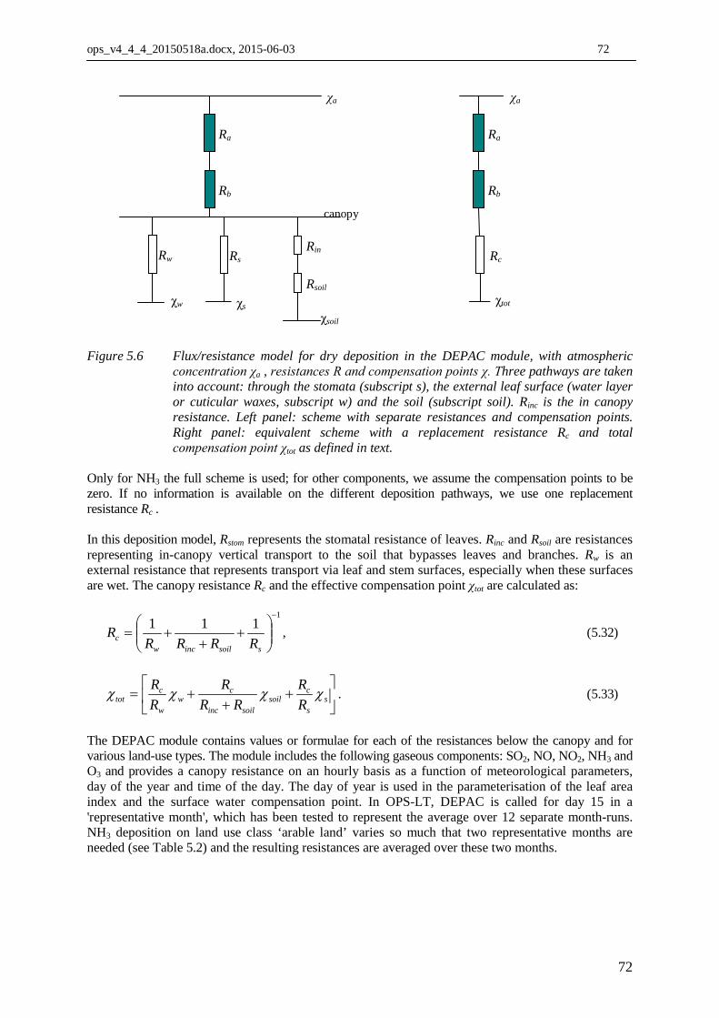
ops_v4_4_4_20150518a.docx, 2015-06-03 72

Figure 5.6 Flux/resistance model for dry deposition in the DEPAC module, with atmospheric

concentration χa , resistances R and compensation points χ. Three pathways are taken into account: through the stomata (subscript s), the external leaf surface (water layer or cuticular waxes, subscript w) and the soil (subscript soil). Rinc is the in canopy resistance. Left panel: scheme with separate resistances and compensation points. Right panel: equivalent scheme with a replacement resistance Rc and total compensation point χtot as defined in text.

Only for NH3 the full scheme is used; for other components, we assume the compensation points to be zero. If no information is available on the different deposition pathways, we use one replacement resistance Rc . In this deposition model, Rstom represents the stomatal resistance of leaves. Rinc and Rsoil are resistances representing in-canopy vertical transport to the soil that bypasses leaves and branches. Rw is an external resistance that represents transport via leaf and stem surfaces, especially when these surfaces are wet. The canopy resistance Rc and the effective compensation point χtot are calculated as:

1

111−

+

++=

ssoilincwc RRRR

R , (5.32)

+

++= s

s

csoil

soilinc

cw

w

ctot R

RRR

RRR χχχχ . (5.33)

The DEPAC module contains values or formulae for each of the resistances below the canopy and for various land-use types. The module includes the following gaseous components: SO2, NO, NO2, NH3 and O3 and provides a canopy resistance on an hourly basis as a function of meteorological parameters, day of the year and time of the day. The day of year is used in the parameterisation of the leaf area index and the surface water compensation point. In OPS-LT, DEPAC is called for day 15 in a 'representative month', which has been tested to represent the average over 12 separate month-runs. NH3 deposition on land use class ‘arable land’ varies so much that two representative months are needed (see Table 5.2) and the resulting resistances are averaged over these two months.

Ra

Rb

Rc

χa

χtot χw

Ra

Rb

Rs

χa

χs

Rw Rin

Rsoil

χsoil

canopy

72

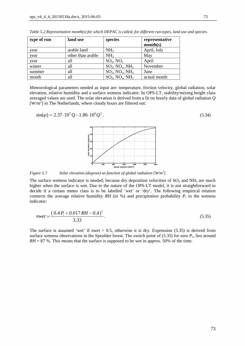
ops_v4_4_4_20150518a.docx, 2015-06-03 73

Table 5.2 Representative month(s) for which DEPAC is called, for different run-types, land use and species.

type of run land use species representative month(s)

year arable land NH3 April, July year other than arable NH3 May year all SO2, NOx April winter all SO2, NOx, NH3 November summer all SO2, NOx, NH3 June month all SO2, NOx, NH3 actual month Meteorological parameters needed as input are: temperature, friction velocity, global radiation, solar elevation, relative humidity and a surface wetness indicator. In OPS-LT, stability/mixing height class averaged values are used. The solar elevation is derived from a fit on hourly data of global radiation Q [W/m2] in The Netherlands, where cloudy hours are filtered out: 263 101.861037.2)sin( QQ ⋅−⋅=ϕ . (5.34)

0 100 200 300 400 500 6000

10

20

30

40

50

global radiation [W/m2]

sola

r ele

vatio

n (d

egre

es)

Figure 5.7 Solar elevation (degrees) as function of global radiation [W/m2].

The surface wetness indicator is needed, because dry deposition velocities of SO2 and NH3 are much higher when the surface is wet. Due to the nature of the OPS-LT model, it is not straightforward to decide if a certain meteo class is to be labelled ‘wet’ or ‘dry’. The following empirical relation connects the average relative humidity RH (in %) and precipitation probability Pr to the wetness indicator:

33.3

)4.0017.04.0( 5−+=

RHPnwet r . (5.35)

The surface is assumed ‘wet’ if nwet > 0.5, otherwise it is dry. Expression (5.35) is derived from surface wetness observations in the Speulder forest. The switch point of (5.35) for zero Pr, lies around RH = 87 %. This means that the surface is supposed to be wet in approx. 50% of the time.

73

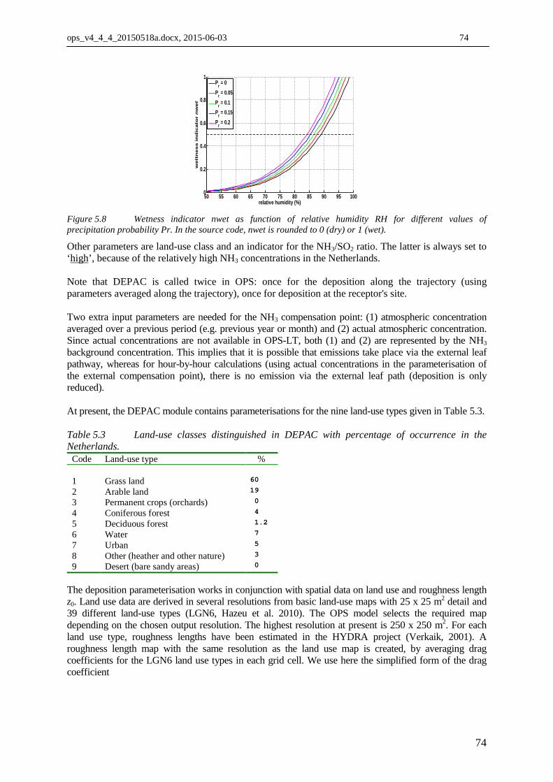
ops_v4_4_4_20150518a.docx, 2015-06-03 74

50 55 60 65 70 75 80 85 90 95 1000

0.2

0.4

0.6

0.8

1

relative humidity (%)w

ett

ness in

dic

ato

r n

wet

Pr = 0Pr = 0.05Pr = 0.1Pr = 0.15Pr = 0.2

Figure 5.8 Wetness indicator nwet as function of relative humidity RH for different values of precipitation probability Pr. In the source code, nwet is rounded to 0 (dry) or 1 (wet).

Other parameters are land-use class and an indicator for the NH3/SO2 ratio. The latter is always set to ‘high’, because of the relatively high NH3 concentrations in the Netherlands. Note that DEPAC is called twice in OPS: once for the deposition along the trajectory (using parameters averaged along the trajectory), once for deposition at the receptor's site. Two extra input parameters are needed for the NH3 compensation point: (1) atmospheric concentration averaged over a previous period (e.g. previous year or month) and (2) actual atmospheric concentration. Since actual concentrations are not available in OPS-LT, both (1) and (2) are represented by the NH3 background concentration. This implies that it is possible that emissions take place via the external leaf pathway, whereas for hour-by-hour calculations (using actual concentrations in the parameterisation of the external compensation point), there is no emission via the external leaf path (deposition is only reduced). At present, the DEPAC module contains parameterisations for the nine land-use types given in Table 5.3. Table 5.3 Land-use classes distinguished in DEPAC with percentage of occurrence in the Netherlands.

Code Land-use type % 1 Grass land 60

2 Arable land 19

3 Permanent crops (orchards) 0

4 Coniferous forest 4

5 Deciduous forest 1.2

6 Water 7

7 Urban 5

8 Other (heather and other nature) 3

9 Desert (bare sandy areas) 0

The deposition parameterisation works in conjunction with spatial data on land use and roughness length z0. Land use data are derived in several resolutions from basic land-use maps with 25 x 25 m2 detail and 39 different land-use types (LGN6, Hazeu et al. 2010). The OPS model selects the required map depending on the chosen output resolution. The highest resolution at present is 250 x 250 m2. For each land use type, roughness lengths have been estimated in the HYDRA project (Verkaik, 2001). A roughness length map with the same resolution as the land use map is created, by averaging drag coefficients for the LGN6 land use types in each grid cell. We use here the simplified form of the drag coefficient

74

ops_v4_4_4_20150518a.docx, 2015-06-03 75

2

0ln

=

zz

Cref

dκ , (5.36)

with κ the Von Karman constant (= 0.4), zref = 10 m. Output of the DEPAC module is the canopy resistance Rc and the total compensation point χtot. In general, after the call to DEPAC, the (hourly) deposition flux F can be computed as: )( totadvF χχ −⋅−= , (5.37) with deposition (exchange) velocity

cba

d RRRv

++=

1. (5.38)

For OPS-LT however, an alternative expression has been chosen: advF χ⋅−= ' , (5.39)

)(1'

'

a

totad

cbad v

RRRv

χχχ −

=++

= , (5.40)

with Rc' the effective canopy resistance, which is also an output of the DEPAC module:

( )( ) .'

−

++=

tota

actotbac

RRRRχχ

χχ (5.41)

In the rare case that Rc' is negative (re-emission over the whole of the stability/mixing height class), OPS-LT resets Rc' to a large value of 1000 s/m. Up to OPS version 4.3.16, the DEPAC routine is called with as argument the dominant land use of the grid cell for which the local deposition has to be calculated. This can give rise to inconsistencies between the aerodynamic resistance Ra and the canopy resistance Rc in case of grid cells with varying land use, because the former is based on the grid averaged roughness value z0. From OPS-version 4.4. on, DEPAC is called for each of the land use classes occurring in the grid cell, upon which the average dry deposition velocity vd is calculated from the resulting Rc values as follows:

icbai

id RRRfv

,

1++

=∑ . (5.42)

with Rc,i the (effective) Rc value of land use class i and fi the fraction of occurrence of class i in the concerned grid cell. Remark that the replacement of vd based on dominant land use by vd based on each of the occurring land use classes is only done for the calculation of vd at the receptor location. For vd along the trajectory path, dominant land use is still used. Further details on DEPAC, such as the parameterisation of different resistances and compensation points, are given in Van Zanten et al. 2010 (available as separate PDF-document depac_yyyymmdd.pdf ).

75

ops_v4_4_4_20150518a.docx, 2015-06-03 76

5.4.2 Dry deposition of NOx In this model NOx represents the sum of NO, NO2, PAN and HNO2. The DEPAC module provides estimates of the canopy resistances of NO and NO2; for HNO2, dry deposition velocities similar to those of SO2 have been suggested by Wesely (1989). Erisman (1992) estimated the average dry deposition of HNO2 in the Netherlands at less than 6 % of the total dry deposition of all oxidised nitrogen components. Dry deposition properties for PAN are assumed to be the same as for NO2. The canopy resistance for NOx is now calculated as:

bac RRa

R −−=1)NO( x (5.43)

with

bacbac

effn

bac

effn

RRRf

RRRr

RRRr

a++

+++

−+

++=

)HNO()NO(1

)NO( 2

HNO,

2

, 2 , (5.44)

where rn,eff is the NO2/NOx ratio and fHNO2 is the fraction of HNO2 in NOx taken at a fixed value of 0.04. Ra is calculated for a height of 4 m. The atmospheric resistances Ra and Rb are included in this calculation only as weighting factors because the calculation of a species weighted Rc has to be carried out on the basis of deposition velocities and not on resistances.

5.4.3 Dry deposition of acidifying aerosols The route to forming particles containing SO4

2-, NO3- and NH4

+ runs through direct gas-to-particle conversion and evaporation of cloud droplets in which conversion has previously taken place. Newly formed particles are usually smaller than 0.01 μm (Aitken particles). If the gas condenses on existing particles (e.g. heterogeneous processes), the median size of these particles will also be relatively small, because small particles have the highest specific surface area. Through processes such as coagulation, small particles will grow and finally be concentrated in a 0.1− 1 μm range, the so-called accumulation mode. Most theoretical models suggest a deposition velocity vd between 0.05 - 0.2 cm/s for this size range and relatively smooth surfaces (z0 < 0.1 m). Data from the literature suggest that for rough surfaces such as forests, the dry deposition velocity will be significantly higher, for example, in the order of 1 cm/s (Voldner et al., 1986; Erisman et al., 1994). A different approach has been followed for acidifying aerosols such as SO4

-, NO3- and NH4

+ than for aerosols or particles in general. One reason is that there is more experimental data available which makes it possible to distinguish between vegetation types; another reason is that particle-sizes are usually small since the particles have been formed in the atmosphere and are thus independent of industrial processes or cleaning equipment. Basically, the dry deposition of particles is modelled using empirical relations. These relations describe the vertical movement of small particles at or within the canopy. The empirical relations can be fitted into a common resistance approach according to Figure 5.9.

76

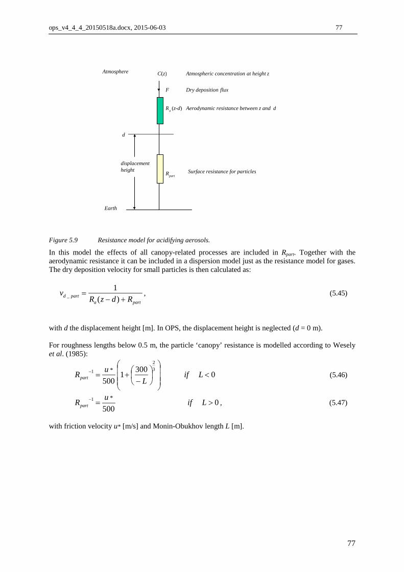
ops_v4_4_4_20150518a.docx, 2015-06-03 77

Figure 5.9 Resistance model for acidifying aerosols.

In this model the effects of all canopy-related processes are included in Rpart. Together with the aerodynamic resistance it can be included in a dispersion model just as the resistance model for gases. The dry deposition velocity for small particles is then calculated as:

parta

partd RdzRv

+−=

)(1

_ , (5.45)

with d the displacement height [m]. In OPS, the displacement height is neglected (d = 0 m). For roughness lengths below 0.5 m, the particle ‘canopy’ resistance is modelled according to Wesely et al. (1985):

03001500

32

1 *<

−

+=− LifL

uRpart (5.46)

0500

*1 >=− LifuRpart , (5.47)

with friction velocity u* [m/s] and Monin-Obukhov length L [m].

R a (z-d)

R part

F

C(z) Atmospheric concentration at height z

Dry deposition flux

Aerodynamic resistance between z and d

Surface resistance for particles

Earth

Atmosphere

d

displacement height

77

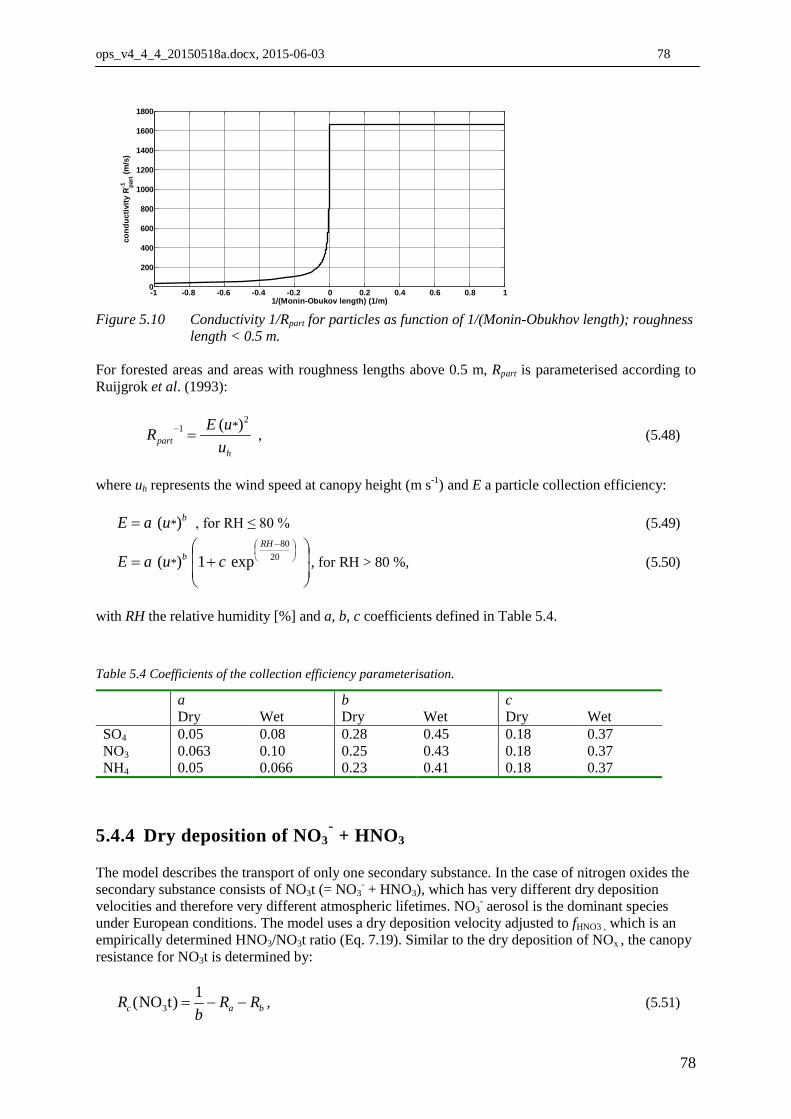
ops_v4_4_4_20150518a.docx, 2015-06-03 78

-1 -0.8 -0.6 -0.4 -0.2 0 0.2 0.4 0.6 0.8 10

200

400

600

800

1000

1200

1400

1600

1800

1/(Monin-Obukov length) (1/m)

cond

uctiv

ity R

part

-1 (m

/s)

Figure 5.10 Conductivity 1/Rpart for particles as function of 1/(Monin-Obukhov length); roughness

length < 0.5 m. For forested areas and areas with roughness lengths above 0.5 m, Rpart is parameterised according to Ruijgrok et al. (1993):

hpart u

uER2

1 )( *=− , (5.48)

where uh represents the wind speed at canopy height (m s-1) and E a particle collection efficiency: buaE )( *= , for RH ≤ 80 % (5.49)

+=

−

2080

exp1)( *

RHb cuaE , for RH > 80 %, (5.50)

with RH the relative humidity [%] and a, b, c coefficients defined in Table 5.4. Table 5.4 Coefficients of the collection efficiency parameterisation.

a b c Dry Wet Dry Wet Dry Wet SO4 0.05 0.08 0.28 0.45 0.18 0.37 NO3 0.063 0.10 0.25 0.43 0.18 0.37 NH4 0.05 0.066 0.23 0.41 0.18 0.37

5.4.4 Dry deposition of NO3- + HNO3

The model describes the transport of only one secondary substance. In the case of nitrogen oxides the secondary substance consists of NO3t (= NO3

- + HNO3), which has very different dry deposition velocities and therefore very different atmospheric lifetimes. NO3

- aerosol is the dominant species under European conditions. The model uses a dry deposition velocity adjusted to fHNO3 , which is an empirically determined HNO3/NO3t ratio (Eq. 7.19). Similar to the dry deposition of NOx , the canopy resistance for NO3t is determined by:

bac RRb

R −−=1)tNO( 3 , (5.51)

78

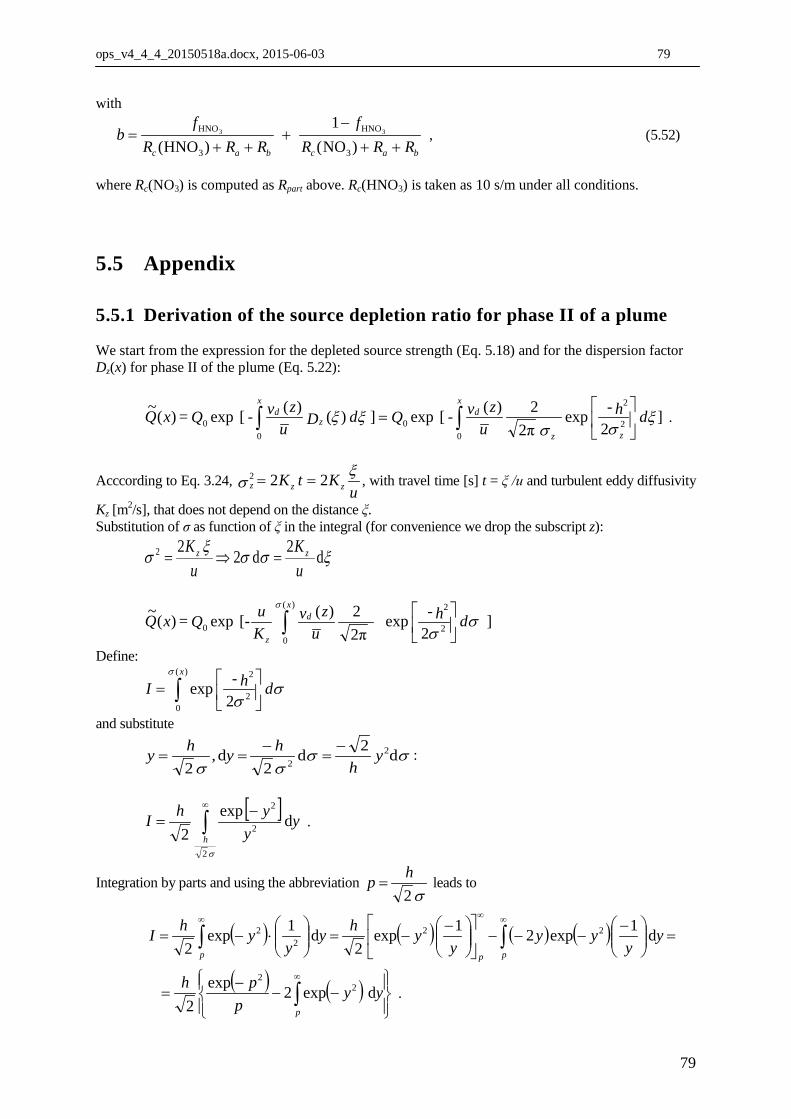
ops_v4_4_4_20150518a.docx, 2015-06-03 79

with

bacbac RRR

fRRR

fb

++−

+++

=)NO(

1)HNO( 3

HNO

3

HNO 33 , (5.52)

where Rc(NO3) is computed as Rpart above. Rc(HNO3) is taken as 10 s/m under all conditions.

5.5 Appendix

5.5.1 Derivation of the source depletion ratio for phase II of a plume We start from the expression for the depleted source strength (Eq. 5.18) and for the dispersion factor Dz(x) for phase II of the plume (Eq. 5.22):

]2

exp2π

2)([exp])()([exp)(~2

2

00

00 x

σσxx d h-

uz v - Q d D u

z v - Q = xQzz

dx

zd

x

= ∫∫ .

Acccording to Eq. 3.24, u

KtK zzzx

σ 222 == , with travel time [s] t = ξ /u and turbulent eddy diffusivity

Kz [m2/s], that does not depend on the distance ξ. Substitution of σ as function of ξ in the integral (for convenience we drop the subscript z):

xσσxσ d2d222

uK

uK zz =⇒=

]2

exp2π2)([-exp)(~

2

2)(

00 d h-

uz v

Ku Q = xQ d

x

z

σσ

σ

∫

Define:

d h- Ix

σσ

σ

= ∫ 2

2)(

0 2exp

and substitute

σσσσ

d2d2

d,2

22

yh

h yhy −=

−== :

[ ] y y

y hIh

dexp2 2

2

2

−= ∫

∞

σ

.

Integration by parts and using the abbreviation σ2

hp = leads to

( ) ( ) ( ) ( ) =

−−−−

−−=

⋅−= ∫∫

∞∞∞

y y

yyy

yhy y

y hIppp

d1exp21exp2

d1exp2

222

2

( ) ( ) y yp

ph

p

−−−

= ∫∞

dexp2exp2

22

.

79

ops_v4_4_4_20150518a.docx, 2015-06-03 80

The integral term, can be approximated as follows: ( )

π4

exp)(erfcπ21)exp(

2

22

++≈=∫

∞

pp

p- pdy -y p

, for p > 0.

(Abramowitz & Stegun (1970), 7.1.13).

( ) ( ) ( ) pp

pp-h

pp

p- p-p

hI =

++−=

++−=

π4

21exp2

π4

exp2exp12 22

22

2

( ) ( ) =

++

−+=

++

−

++

=

π4

π4

exp2

π4

2π4

exp2 2

2

2

2

22

ppp

ppp-h

ppp

pppp-h

( ) ( ) =

++

−+=

++

++

−+

= 2

2

22

2

2

22

π4

π4

exp2

π4

π4

π4

exp2

22

ppp

ppp-h

ppp

ppppp-h

( ) ( ) ,exp2

π4

π4

exp2

22

2

2p

p-h

ppp

p-h β=

++

= with

2

2

22

2

2

2

2

2

2 811

8

1π411

1π4

π4

π4

++

=

++

=

++

=

hhp

p

pppσp

σβ .

The depleted source strength can be written as:

( ) ].exp22π

2)([-exp]2π2)([-exp)(~ 2

00 p

p-h u

z v Ku Q I

uz v

Ku Q= xQ d

z

d

z

β=

Substitute 2

21 σ

xuK z = and

σ2hp = :

=

]

2exp2

22π2)(2[-exp)(~

2

2

20 h-h

h u

z v x Q =xQ d

σβσ

σ

]2

exp)(2π4[-exp 2

2

0 h- u

z v x Q = d

σ

βσ

.

The source depletion ratio is:

80

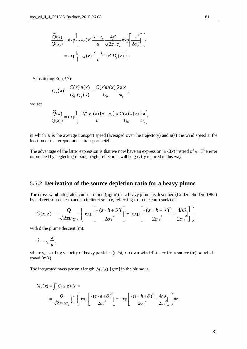
ops_v4_4_4_20150518a.docx, 2015-06-03 81

,)(2)(exp

2exp

24)(exp

)()(~

2

2

−

=

−−=

xDu

xx z v-

hu

xx z v- xQxQ

zs

d

zz

sd

s

β

σσpβ

Substituting Eq. (3.7):

m

xQ

xuxC = xD QxuxC = xD

syz

π2)()()()()()(

00,

we get:

( ) .π2)()()(2exp)()(~

0

−

=s

sd

s mQxuxCx

uxxzv-

xQxQ β

in which u is the average transport speed (averaged over the trajectory) and u(x) the wind speed at the location of the receptor and at transport height. The advantage of the latter expression is that we now have an expression in C(x) instead of σz. The error introduced by neglecting mixing height reflections will be greatly reduced in this way.

5.5.2 Derivation of the source depletion ratio for a heavy plume The cross-wind integrated concentration (µg/m2) in a heavy plume is described (Onderdelinden, 1985) by a direct source term and an indirect source, reflecting from the earth surface:

+

+

+ hh+z- + h-z- u

Q = zxCzzzz σδ

σδ

σδ

σ 24

2)(exp

2)(exp

2π),( 22

2

2

2

,

with δ the plume descent (m):

uxvs=δ ,

where vs : settling velocity of heavy particles (m/s), x: down-wind distance from source (m), u: wind speed (m/s). The integrated mass per unit length )(xM [g/m] in the plume is

.

24

2)(exp

2)(exp

2π

),()(

0 22

2

2

2

0

dz hh+z- + h-z- u

Q

= dzzxCxM

zzzz∫

∫∞

∞

+

+

+=

=

σδ

σδ

σδ

σ

81

ops_v4_4_4_20150518a.docx, 2015-06-03 82

Substituting σ

δ

2

)(

z

h-zy += in the first and

σ

δ

2

)(

z

hzy ++= in the second term, we get

( ) ( )

⋅

+= ∫∫

∞∞

2

2

1

2 exp24expexp

π)( 2 p

zp

dy y- hdy y- u

Q xMσδ

,

with z

h-pσδ

21+

= , z

hpσδ

22+

= .

These integrals can be expressed in terms of complementary error functions and are approximated as follows:

( )

π4

exp)(erfcπ21)exp(

2

22

++≈=∫

∞

pp

p- pdy -y p

, for p > 0

( )

π4

expπ)exp()exp()exp(2

2222

++−−≈−= ∫∫∫ ∞−

∞

∞−

∞

pp

p- dy -y dy -y dy -y p

p, for p < 0.

(Abramowitz & Stegun (1970), 7.1.13). Note that

( ) ( ) ( ) ( )212

z

2

2z

2

2z

222

z

exp2

exp22

4expexp24exp p- hhhp- h

=

+−−=

+−=⋅

σδ

σδ

σδ

σδ

.

( ) ( )

( ) ( ) 0,

π4

exp

π4

expπ

π4

exp24exp

π4

expπ

)(

1222

21

211

21

222

22

2z2

11

21

≥

+++

++=

=

++⋅

+

++≈

ppp

p-

pp

p- u

Q

pp

p- h

pp

p- u

Q xMσδ

( ) ( ) .0,

π4

exp

π4

expππ

)( 1222

21

211

21 <

+++

++−−≈ p

pp

p-

pp

p- u

Q xM

We approximate the depleted source strength Q~ (g/s) as follows:

).()()(1~0

xMuxMtx dM

tQ

x

=≈= ∫ xx

The source depletion ratio's are:

82

ops_v4_4_4_20150518a.docx, 2015-06-03 83

( ) hpppp

p-

Q

xQ≥

+++

++≈ δ,

π4

1

π4

1expπ1)(~

222

211

21

( ) .,

π4

1

π4

1expπ11)(~

222

211

21 h

ppppp-

QxQ

<

++−

++−−≈ δ

The concentration at the surface z = 0 is

.

2)(exp

2π2

24)(exp

2)(exp

2π)0,(

2

2

2

2

2

2

−−=

=

++−

+−−

σ

δσ

σ

δδ

σ

δσ

zz

zzz

h u

Q

hh + h u

Q =xC

The flux F at the surface z = 0 is

( ) ( )

.2

)(exp2π2

2)(exp

2π

)0,()0,(

2

2

222

2

0

−−−

+

+−

−

−−−=

=−∂∂

−=

h u

Qv

h K+hK h u

Q

xCv zCK = xF

zzs

zz

zz

zz

sz

z

σδ

σ

σδ

σδ

σδ

σ

Substituting for the eddy diffusivity Kz [m2/s] σ zz xuK 2

21

= and plume descent uxvs=δ , we get:

)0,(21

2)(exp

2π)0,( 2

2

xCv h u

Qv = xF szz

s −=

−−−

σδ

σ.

In other words, the deposition velocity is half the settling velocity.

5.6 References Abramowitz, Milton; Stegun, Irene A., eds. (1970), Handbook of Mathematical Functions with Formulas, Graphs,

and Mathematical Tables, New York: Dover Publications, SBN 486-61272-4, see also http://people.math.sfu.ca/~cbm/aands/

Beljaars A.C.M. and Holtslag A.A.M. (1990) A software library for the calculation of surface fluxes over land and sea. Environ. Software 5, 60-68.

Brutsaert W.P. (1975) The roughness length of water vapour, sensible heat and other scalars. J. Atmos. Sci. 32, 2028-2031.

Duyzer J.H. and Fowler D. (1994) Modelling land atmosphere exchange of gaseous oxides of nitrogen in Europe. Tellus 46B, 353-372.

83

ops_v4_4_4_20150518a.docx, 2015-06-03 84

Erisman J.W. (1992) Atmospheric deposition of acidifying compounds in the Netherlands. [PhD thesis]. Utrecht University, the Netherlands.

Erisman J.W., Pul W.A.J. van and Wyers G.P (1994) Parameterization of surface resistance for the quantification of atmospheric deposition of acidifying pollutants and ozone. Atmospheric Environment 28, 2595-2607.

Garratt J.R. and Hicks B.B. (1973) Momentum, heat and water vapour transfer to and from natural and artificial surfaces. Q. J. R. Meteorol. Soc. 99, 680-687.

Hazeu, G.W., Schuiling, C., Dorland, G.J., Oldengarm, J. & H.A. Gijsbertse, 2010. Landelijk Grondgebruiks-bestand Nederland versie 6 (LGN6). Vervaardiging, nauwkeurigheid en gebruik. Wageningen, Alterra. Alterra-rapport 2012 (http://webdocs.alterra.wur.nl/internet/geoinformatie/lgn/AlterraRapport2012.pdf). See also http://www.alterra.wur.nl/NL/onderzoek/Werkveld+Geoinformatie/LGN/bestand_LGN6/.

Hicks B.B., Baldocchi D.D. Meyers T.P., Hosker Jr. R.P. and Matt D.R. (1987) A preliminary multiple resistance routine for deriving dry deposition velocities from measured quantities. Water Air Soil Pollut. 36, 311-330.

Hicks B.B., Matt D.R. and McMillen R.T. (1989) A micrometeorological investigation of surface exchange of O3, SO2 and NO2: a case study. Boundary-Layer Meteorol. 47, 321-336.

Horst T. W. (1977) A surface depletion model for deposition from a Gaussian plume. Atmospheric Environment 11, 41-46.

Nieuwstadt F.T.M. (1984) Some aspects of the turbulent stable boundary layer. Boundary-Layer Meteorol. 30, 31-55.

Onderdelinden D., Jaarsveld J.A. van and Egmond N.D. van (1984) Bepaling van de depositie van zwavelverbindingen in Nederland. RIVM, Bilthoven, the Netherlands. Report no. 842017001.

Onderdelinden (1985): Source depletion model, personal communication in OPS archive. Ruijgrok W., Nicholson K.W., and Davidson C.I. (1993) Dry deposition of particles. In: Lövblad G., Erisman J.W.

and Fowler D., editors. Models and methods for the quantification of atmospheric input to ecosystems. Nordic Council of Ministers, Copenhagen.

Scriven R.A. and Fisher B.E.A. (1975) The long range transport of airborne material and its removal by deposition and washout - I. General considerations. Atmospheric Environment 9, 49-58.

Slinn W.G.N (1982) Predictions for particle deposition to vegetative surfaces. Atmospheric Environment 16, 1785-1794.

Van Dop H., Ridder T.B., Tonkelaar J.F. den and Egmond N.D. van (1980) Sulfur dioxide measurements on the 213 metre tower at Cabauw, the Netherlands. Atmospheric Environment 14, 933-946.

Van Egmond N.D. and Kesseboom H. (1983) Mesoscale air pollution dispersion models I: Eulerian Grid Model. Atmospheric Environment 17, 257-265.

Van Jaarsveld J.A., Pul W.A.J. van and Leeuw F.A.A.M. de (1994) Modelling the long range transport and deposition of persistent organic pollutants over Europe and its surrounding marine areas. In: Gryning S.E. and Millán M.M., editors. Air pollution modelling and its application X. Plenum Press, New York. p. 143-155.

Van Zanten M.C., Sauter F.J., Wichink Kruit R.J., van Jaarsveld J.A., van Pul W.A.J.: Description of the DEPAC module, Dry deposition modelling with DEPAC_GCN2010, RIVM report 680180001, RIVM, Bilthoven, 2010

Verkaik, J.W. (2001): A method for the geographical interpolation of wind speed over heterogeneous terrain, KNMI report, http://www.knmi.nl/samenw/hydra/documents/geograph/interpol.pdf

Voldner E.C., Barrie L.A. and Sirois A. (1986) A literature review of dry deposition of oxides of sulphur and nitrogen with emphasis on long-range transport modelling in North America. Atmospheric Environment 20, 2101-2123.

Wesely M.L. and Hicks, B.B. (1977) Some factors that effect the deposition rates of sulfur dioxide and similar gases on vegetation. J. Air Pollut. Control Assoc. 27, 1110-1116.

Wesely M.L., Cook D.R., Hart R.L. and Speer R.E. (1985) Measurements and parameterization of particulate sulfur dry deposition over grass. J.Geophys. Res., 90(D1):2131-2143.

Wesely M.L. (1989) Parameterization of surface resistances to gaseous dry deposition in regional scale numerical models. Atmospheric Environment 23, 1293-1304.

Wichink Kruit, R.J., W.A.J. van Pul, R.P. Otjes, P. Hofschreuder, A.F.G. Jacobs and A.A.M. Holtslag (2007) Ammonia fluxes and derived canopy compensation points over non-fertilized agricultural grassland in The Netherlands using the new gradient ammonia - high accuracy - monitor (GRAHAM). Atmospheric Environment 41: 1275-1287.

84

ops_v4_4_4_20150518a.docx, 2015-06-03 85

Wichink Kruit, R.J., W.AJ. van Pul, F.J. Sauter, M. van den Broek, E. Nemitz, M.A. Sutton, M. Krol and A.A.M. Holtslag (2010) Modeling the surface-atmosphere exchange of ammonia. Atmospheric Environment, Vol. 44, 7: 877-1004.

85

ops_v4_4_4_20150518a.docx, 2015-06-03 86

6. Wet deposition Although the wet deposition process is complex, an attempt has been made to use as simple a parameterisation as possible, which can be applied more-or-less universally for both long-range transport and more local deposition. Two main scavenging processes are distinguished in this model: below-cloud scavenging and in-cloud scavenging. Below-cloud scavenging is important for scavenging from plumes close to sources in situations where there is no interaction with clouds yet. The rate limiting process is formed by diffusion of the substance through the pseudo-laminar air layer around the falling raindrop (Levine and Schwartz, 1982). In general, in-cloud processes are responsible for the highest wet deposition loads (Hales, 1978).

6.1 In-cloud scavenging Natural storms are complex in their microphysical and dynamical structure and relations between concentrations in precipitation and the surrounding air are very variable (Barrie, 1992). Modelling of the precipitation process in transport models is usually done using either linear scavenging ratios or a numerical approach, including all the physical and chemical details of the process; there are hardly any solutions in between. The present model describes the in-cloud scavenging as a statistical process rather than as single events. The process is viewed as a discontinuous flow reactor, in which chemicals in air entering a precipitation system are transferred to other chemicals and/or precipitation. At a large distance from the source, where the pollutant is well vertically mixed and has also had the opportunity to penetrate into the cloud base, the scavenging rate of a pollutant Λin (h-1) is given by:

hRW = Λ i

in , (6.1)

where Ri is the precipitation intensity [m h-1], W the ratio between the (initial) concentration in precipitation and the (initial) concentration in air [-], both on a weight/volume basis and at the ground level. Parameter h is the height over which wet deposition takes place [m]:

=otherwise,,

layermixingtheabovecompletelyplume,2

i

z

zh

σ (6.2)

with σz the vertical dispersion length of the plume [m] and zi the mixing height [m]. This formulation, when used with an empirically determined W, integrates, in fact, all the processes in and below the cloud. User specified substance Either a scavenging ratio W [-] or a scavenging rate Λin [h-1](1) is to be specified by the user. W may have been determined either empirically from concentrations in rainwater and air or theoretically via Henry’s constant. SO2 Scavenging ratios for SO2 have been determined from experiments. Haul (1978) derived a ratio of 8∙104 from hourly measurements of SO2 and rainfall rates in the UK. Other authors used simultaneous observations of SO2 and SO4

2- in air and precipitation to estimate scavenging ratios of both SO2 and SO42-

(e.g. Misra et al., 1985; Chan and Chung, 1986). Chan and Chung report annual scavenging ratios of 4.3∙105 (SO4

2-), 4.6∙104 (SO2), 4.7∙105 (NO3-) and 4.7∙105 (HNO3) for rural sites in the province of

Ontario, Canada. Barrie (1981) expresses the scavenging ratio of SO2 on the basis of equilibrium chemistry:

(1) in OPS input file to be specified in %/h

86

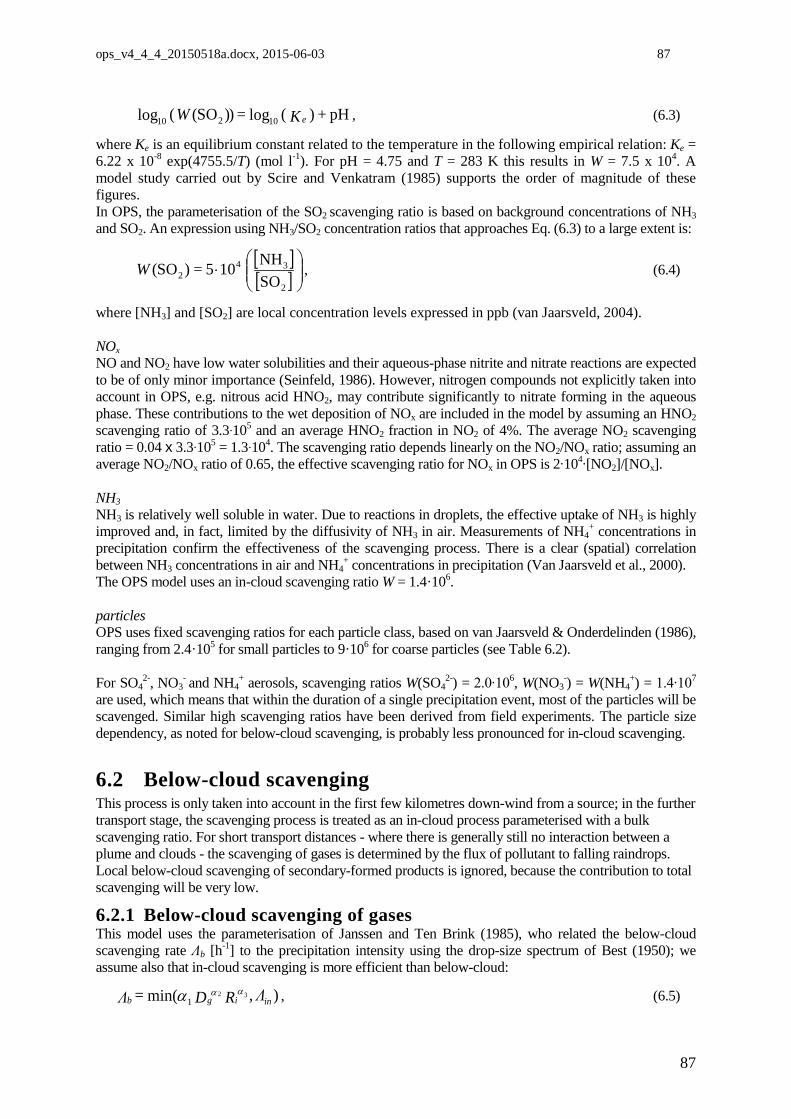
ops_v4_4_4_20150518a.docx, 2015-06-03 87

pH)( log))SO((log 10210 + K = W e , (6.3)

where Ke is an equilibrium constant related to the temperature in the following empirical relation: Ke = 6.22 x 10-8 exp(4755.5/T) (mol l-1). For pH = 4.75 and T = 283 K this results in W = 7.5 x 104. A model study carried out by Scire and Venkatram (1985) supports the order of magnitude of these figures. In OPS, the parameterisation of the SO2 scavenging ratio is based on background concentrations of NH3 and SO2. An expression using NH3/SO2 concentration ratios that approaches Eq. (6.3) to a large extent is:

[ ][ ]

⋅

2

342 SO

NH105)SO( =W , (6.4)

where [NH3] and [SO2] are local concentration levels expressed in ppb (van Jaarsveld, 2004). NOx NO and NO2 have low water solubilities and their aqueous-phase nitrite and nitrate reactions are expected to be of only minor importance (Seinfeld, 1986). However, nitrogen compounds not explicitly taken into account in OPS, e.g. nitrous acid HNO2, may contribute significantly to nitrate forming in the aqueous phase. These contributions to the wet deposition of NOx are included in the model by assuming an HNO2 scavenging ratio of 3.3∙105 and an average HNO2 fraction in NO2 of 4%. The average NO2 scavenging ratio = 0.04 x 3.3∙105 = 1.3∙104. The scavenging ratio depends linearly on the NO2/NOx ratio; assuming an average NO2/NOx ratio of 0.65, the effective scavenging ratio for NOx in OPS is 2∙104∙[NO2]/[NOx]. NH3 NH3 is relatively well soluble in water. Due to reactions in droplets, the effective uptake of NH3 is highly improved and, in fact, limited by the diffusivity of NH3 in air. Measurements of NH4

+ concentrations in precipitation confirm the effectiveness of the scavenging process. There is a clear (spatial) correlation between NH3 concentrations in air and NH4

+ concentrations in precipitation (Van Jaarsveld et al., 2000). The OPS model uses an in-cloud scavenging ratio W = 1.4·106. particles OPS uses fixed scavenging ratios for each particle class, based on van Jaarsveld & Onderdelinden (1986), ranging from 2.4·105 for small particles to 9·106 for coarse particles (see Table 6.2). For SO4

2-, NO3- and NH4

+ aerosols, scavenging ratios W(SO42-) = 2.0∙106, W(NO3

-) = W(NH4+) = 1.4∙107

are used, which means that within the duration of a single precipitation event, most of the particles will be scavenged. Similar high scavenging ratios have been derived from field experiments. The particle size dependency, as noted for below-cloud scavenging, is probably less pronounced for in-cloud scavenging.

6.2 Below-cloud scavenging This process is only taken into account in the first few kilometres down-wind from a source; in the further transport stage, the scavenging process is treated as an in-cloud process parameterised with a bulk scavenging ratio. For short transport distances - where there is generally still no interaction between a plume and clouds - the scavenging of gases is determined by the flux of pollutant to falling raindrops. Local below-cloud scavenging of secondary-formed products is ignored, because the contribution to total scavenging will be very low.

6.2.1 Below-cloud scavenging of gases This model uses the parameterisation of Janssen and Ten Brink (1985), who related the below-cloud scavenging rate Λb [h-1] to the precipitation intensity using the drop-size spectrum of Best (1950); we assume also that in-cloud scavenging is more efficient than below-cloud:

),min( 321 ini

gb ΛR D = Λ ααα , (6.5)

87

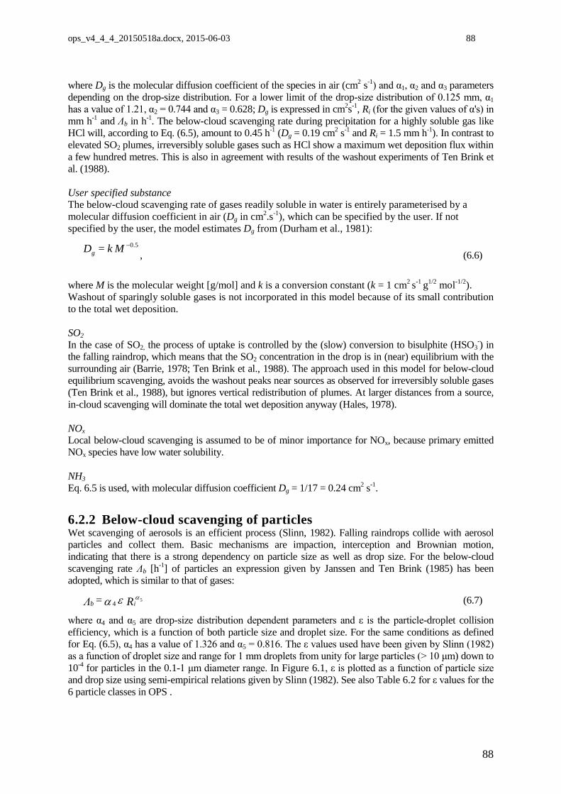
ops_v4_4_4_20150518a.docx, 2015-06-03 88

where Dg is the molecular diffusion coefficient of the species in air (cm2 s-1) and α1, α2 and α3 parameters depending on the drop-size distribution. For a lower limit of the drop-size distribution of 0.125 mm, α1 has a value of 1.21, α2 = 0.744 and α3 = 0.628; Dg is expressed in cm2s-1, Ri (for the given values of α's) in mm h-1 and Λb in h-1. The below-cloud scavenging rate during precipitation for a highly soluble gas like HCl will, according to Eq. (6.5), amount to 0.45 h-1 (Dg = 0.19 cm2 s-1 and Ri = 1.5 mm h-1). In contrast to elevated SO2 plumes, irreversibly soluble gases such as HCl show a maximum wet deposition flux within a few hundred metres. This is also in agreement with results of the washout experiments of Ten Brink et al. (1988). User specified substance The below-cloud scavenging rate of gases readily soluble in water is entirely parameterised by a molecular diffusion coefficient in air (Dg in cm2.s-1), which can be specified by the user. If not specified by the user, the model estimates Dg from (Durham et al., 1981):

5.0−Mk = Dg , (6.6)

where M is the molecular weight [g/mol] and k is a conversion constant (k = 1 cm2 s-1 g1/2 mol-1/2). Washout of sparingly soluble gases is not incorporated in this model because of its small contribution to the total wet deposition. SO2 In the case of SO2, the process of uptake is controlled by the (slow) conversion to bisulphite (HSO3

-) in the falling raindrop, which means that the SO2 concentration in the drop is in (near) equilibrium with the surrounding air (Barrie, 1978; Ten Brink et al., 1988). The approach used in this model for below-cloud equilibrium scavenging, avoids the washout peaks near sources as observed for irreversibly soluble gases (Ten Brink et al., 1988), but ignores vertical redistribution of plumes. At larger distances from a source, in-cloud scavenging will dominate the total wet deposition anyway (Hales, 1978). NOx Local below-cloud scavenging is assumed to be of minor importance for NOx, because primary emitted NOx species have low water solubility. NH3 Eq. 6.5 is used, with molecular diffusion coefficient Dg = 1/17 = 0.24 cm2 s-1.

6.2.2 Below-cloud scavenging of particles Wet scavenging of aerosols is an efficient process (Slinn, 1982). Falling raindrops collide with aerosol particles and collect them. Basic mechanisms are impaction, interception and Brownian motion, indicating that there is a strong dependency on particle size as well as drop size. For the below-cloud scavenging rate Λb [h-1] of particles an expression given by Janssen and Ten Brink (1985) has been adopted, which is similar to that of gases:

R = Λ ibαεα 54 (6.7)

where α4 and α5 are drop-size distribution dependent parameters and ε is the particle-droplet collision efficiency, which is a function of both particle size and droplet size. For the same conditions as defined for Eq. (6.5), α4 has a value of 1.326 and α5 = 0.816. The ε values used have been given by Slinn (1982) as a function of droplet size and range for 1 mm droplets from unity for large particles (> 10 μm) down to 10-4 for particles in the 0.1-1 μm diameter range. In Figure 6.1, ε is plotted as a function of particle size and drop size using semi-empirical relations given by Slinn (1982). See also Table 6.2 for ε values for the 6 particle classes in OPS .

88

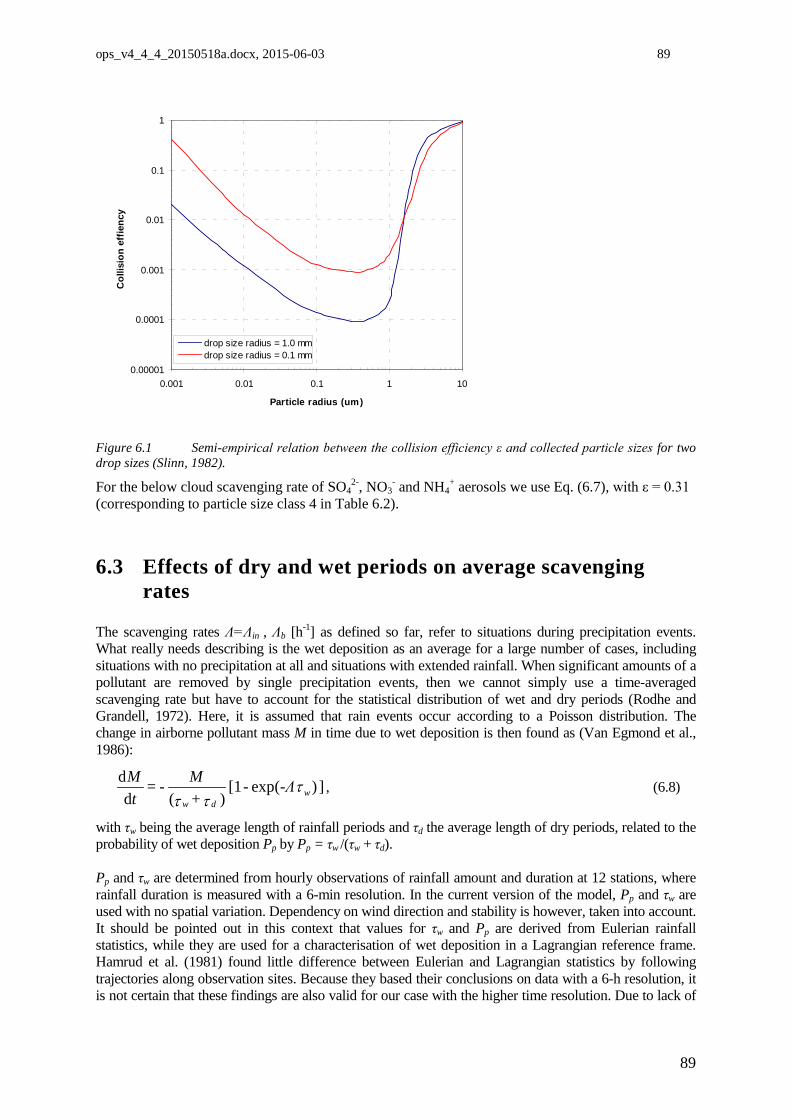
ops_v4_4_4_20150518a.docx, 2015-06-03 89

0.00001

0.0001

0.001

0.01

0.1

1

0.001 0.01 0.1 1 10

Particle radius (um)

Col

lisio

n ef

fienc

y

drop size radius = 1.0 mmdrop size radius = 0.1 mm

Figure 6.1 Semi-empirical relation between the collision efficiency ε and collected particle sizes for two drop sizes (Slinn, 1982).

For the below cloud scavenging rate of SO42-, NO3

- and NH4+ aerosols we use Eq. (6.7), with ε = 0.31

(corresponding to particle size class 4 in Table 6.2).

6.3 Effects of dry and wet periods on average scavenging rates

The scavenging rates Λ=Λin , Λb [h-1] as defined so far, refer to situations during precipitation events. What really needs describing is the wet deposition as an average for a large number of cases, including situations with no precipitation at all and situations with extended rainfall. When significant amounts of a pollutant are removed by single precipitation events, then we cannot simply use a time-averaged scavenging rate but have to account for the statistical distribution of wet and dry periods (Rodhe and Grandell, 1972). Here, it is assumed that rain events occur according to a Poisson distribution. The change in airborne pollutant mass M in time due to wet deposition is then found as (Van Egmond et al., 1986):

])(exp[1)(d

dw

dw-Λ -

+ M - =

tM τ

ττ, (6.8)

with τw being the average length of rainfall periods and τd the average length of dry periods, related to the probability of wet deposition Pp by Pp = τw /(τw + τd). Pp and τw are determined from hourly observations of rainfall amount and duration at 12 stations, where rainfall duration is measured with a 6-min resolution. In the current version of the model, Pp and τw are used with no spatial variation. Dependency on wind direction and stability is however, taken into account. It should be pointed out in this context that values for τw and Pp are derived from Eulerian rainfall statistics, while they are used for a characterisation of wet deposition in a Lagrangian reference frame. Hamrud et al. (1981) found little difference between Eulerian and Lagrangian statistics by following trajectories along observation sites. Because they based their conclusions on data with a 6-h resolution, it is not certain that these findings are also valid for our case with the higher time resolution. Due to lack of

89

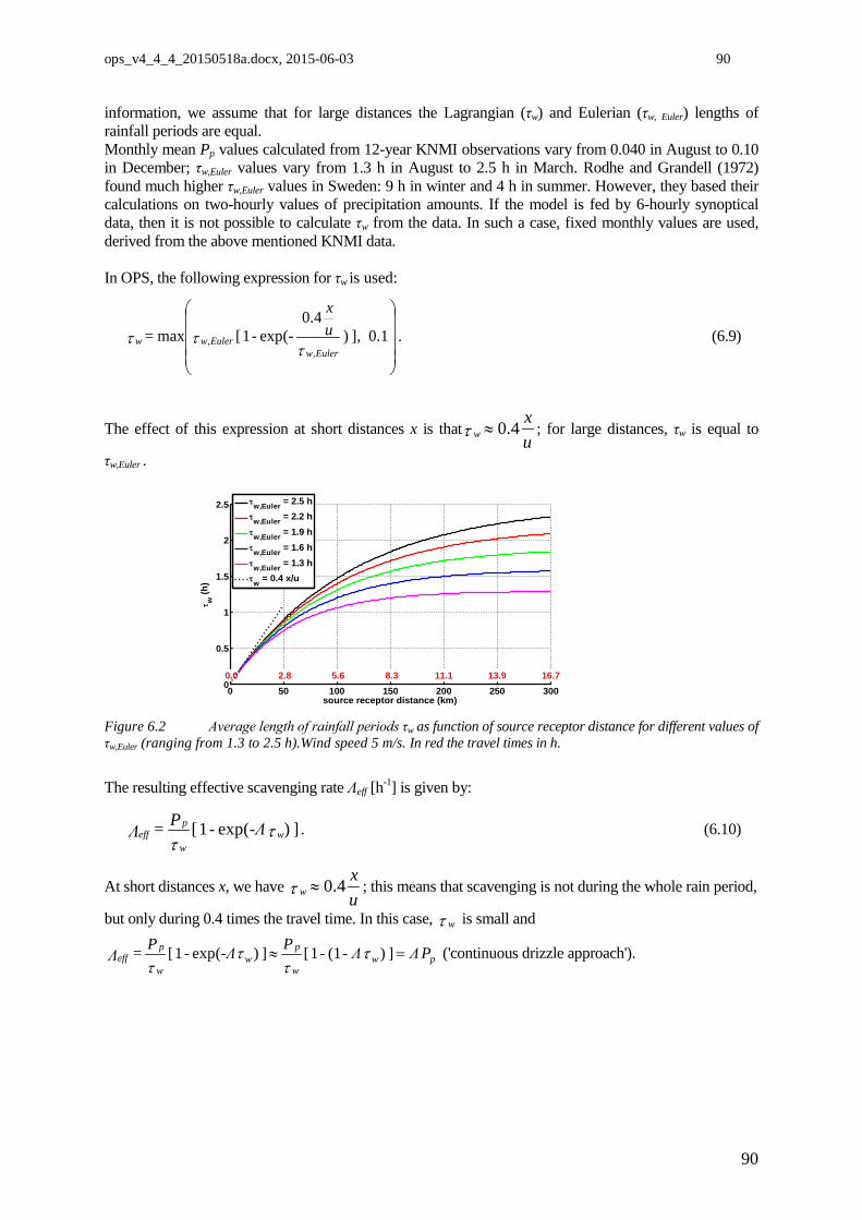
ops_v4_4_4_20150518a.docx, 2015-06-03 90

information, we assume that for large distances the Lagrangian (τw) and Eulerian (τw, Euler) lengths of rainfall periods are equal. Monthly mean Pp values calculated from 12-year KNMI observations vary from 0.040 in August to 0.10 in December; τw,Euler values vary from 1.3 h in August to 2.5 h in March. Rodhe and Grandell (1972) found much higher τw,Euler values in Sweden: 9 h in winter and 4 h in summer. However, they based their calculations on two-hourly values of precipitation amounts. If the model is fed by 6-hourly synoptical data, then it is not possible to calculate τw from the data. In such a case, fixed monthly values are used, derived from the above mentioned KNMI data. In OPS, the following expression for τw is used:

0.1], )0.4

(exp1 [max,

, ux

- - = Eulerw

Eulerwwτ

ττ . (6.9)

The effect of this expression at short distances x is thatux

w 4.0≈τ ; for large distances, τw is equal to

τw,Euler .

0 50 100 150 200 250 3000

0.5

1

1.5

2

2.5

source receptor distance (km)

τ w (h

)

0.0 2.8 5.6 8.3 11.1 13.9 16.7

τw,Euler = 2.5 hτw,Euler = 2.2 hτw,Euler = 1.9 hτw,Euler = 1.6 hτw,Euler = 1.3 hτw = 0.4 x/u

Figure 6.2 Average length of rainfall periods τw as function of source receptor distance for different values of τw,Euler (ranging from 1.3 to 2.5 h).Wind speed 5 m/s. In red the travel times in h.

The resulting effective scavenging rate Λeff [h-1] is given by:

] )(exp1 [ ττ

ww

peff -Λ - P = Λ . (6.10)

At short distances x, we have ux

w 4.0≈τ ; this means that scavenging is not during the whole rain period,

but only during 0.4 times the travel time. In this case, τ w is small and

pww

pw

w

peff PΛ Λ- - P -Λ - P = Λ =≈ ] )(11 [ ] )(exp1 [ τ

ττ

τ ('continuous drizzle approach').

90

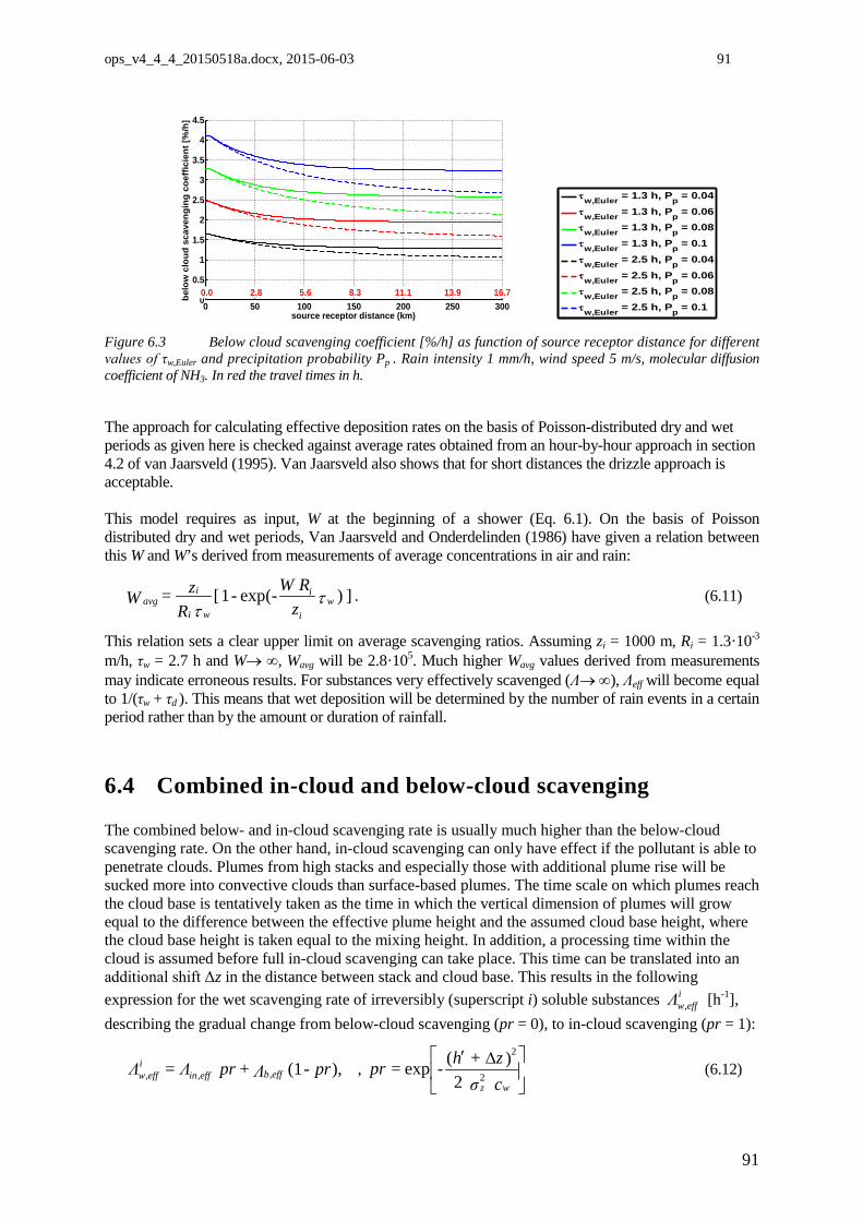
ops_v4_4_4_20150518a.docx, 2015-06-03 91

0 50 100 150 200 250 3000

0.5

1

1.5

2

2.5

3

3.5

4

4.5

source receptor distance (km)

belo

w c

loud

sca

veng

ing

coef

ficie

nt [%

/h]

0.0 2.8 5.6 8.3 11.1 13.9 16.7

τw,Euler = 1.3 h, Pp = 0.04τw,Euler = 1.3 h, Pp = 0.06τw,Euler = 1.3 h, Pp = 0.08τw,Euler = 1.3 h, Pp = 0.1τw,Euler = 2.5 h, Pp = 0.04τw,Euler = 2.5 h, Pp = 0.06τw,Euler = 2.5 h, Pp = 0.08τw,Euler = 2.5 h, Pp = 0.1

Figure 6.3 Below cloud scavenging coefficient [%/h] as function of source receptor distance for different values of τw,Euler and precipitation probability Pp . Rain intensity 1 mm/h, wind speed 5 m/s, molecular diffusion coefficient of NH3. In red the travel times in h.

The approach for calculating effective deposition rates on the basis of Poisson-distributed dry and wet periods as given here is checked against average rates obtained from an hour-by-hour approach in section 4.2 of van Jaarsveld (1995). Van Jaarsveld also shows that for short distances the drizzle approach is acceptable. This model requires as input, W at the beginning of a shower (Eq. 6.1). On the basis of Poisson distributed dry and wet periods, Van Jaarsveld and Onderdelinden (1986) have given a relation between this W and W’s derived from measurements of average concentrations in air and rain:

] )(exp1 [ zRW- -

Rz = W w

i

i

wi

iavg τ

τ. (6.11)

This relation sets a clear upper limit on average scavenging ratios. Assuming zi = 1000 m, Ri = 1.3·10-3

m/h, τw = 2.7 h and W→ ∞, Wavg will be 2.8·105. Much higher Wavg values derived from measurements may indicate erroneous results. For substances very effectively scavenged (Λ→ ∞), Λeff will become equal to 1/(τw + τd ). This means that wet deposition will be determined by the number of rain events in a certain period rather than by the amount or duration of rainfall.

6.4 Combined in-cloud and below-cloud scavenging The combined below- and in-cloud scavenging rate is usually much higher than the below-cloud scavenging rate. On the other hand, in-cloud scavenging can only have effect if the pollutant is able to penetrate clouds. Plumes from high stacks and especially those with additional plume rise will be sucked more into convective clouds than surface-based plumes. The time scale on which plumes reach the cloud base is tentatively taken as the time in which the vertical dimension of plumes will grow equal to the difference between the effective plume height and the assumed cloud base height, where the cloud base height is taken equal to the mixing height. In addition, a processing time within the cloud is assumed before full in-cloud scavenging can take place. This time can be translated into an additional shift Δz in the distance between stack and cloud base. This results in the following expression for the wet scavenging rate of irreversibly (superscript i) soluble substances i

effwΛ , [h-1], describing the gradual change from below-cloud scavenging (pr = 0), to in-cloud scavenging (pr = 1):

pr - Λ + pr Λ = Λ effbeffini

effw ,)(1,,, ,

∆′

c σ z + h-pr =

wz2

2

2)(exp (6.12)

91

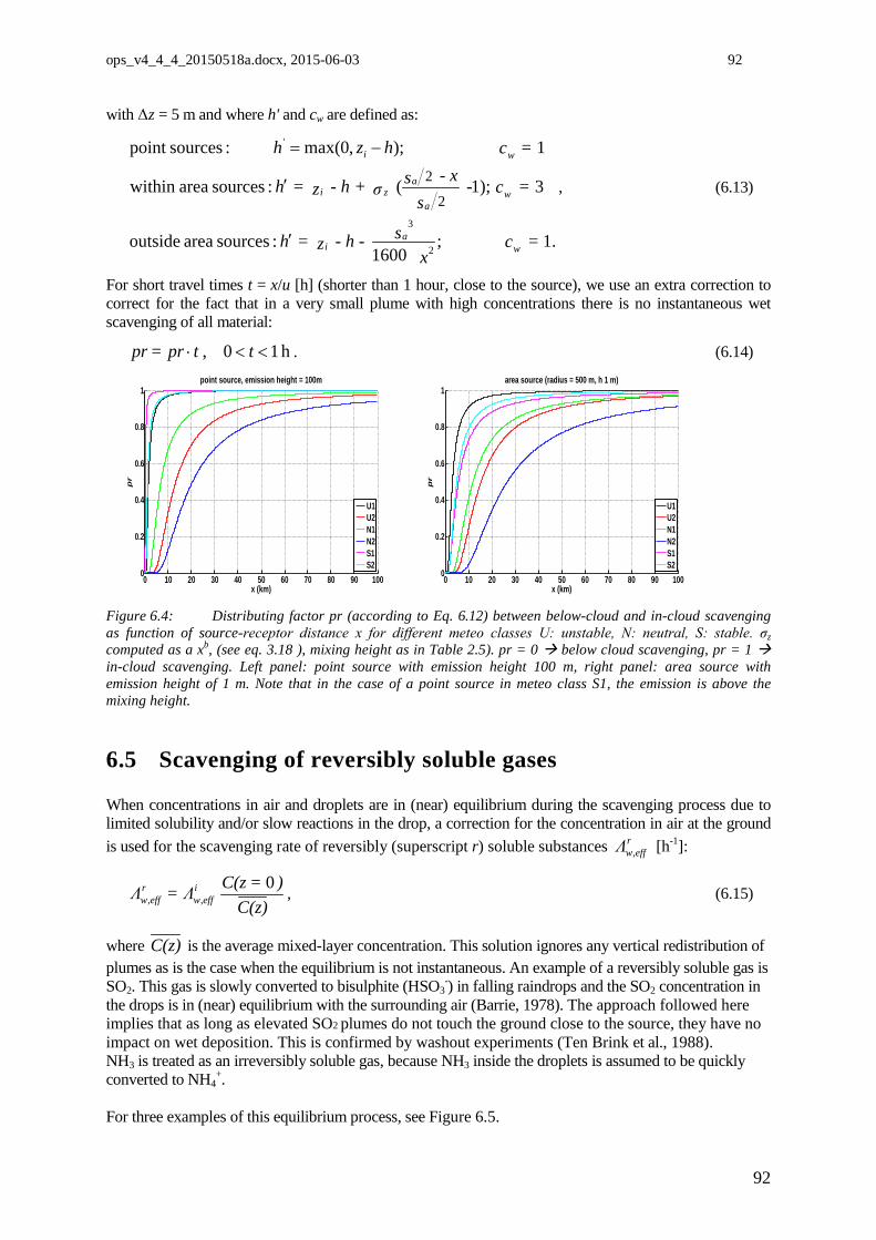
ops_v4_4_4_20150518a.docx, 2015-06-03 92

with Δz = 5 m and where h' and cw are defined as:

1.;1600

:sources area outside

31);( :sources areawithin

1 = );,0max(:sourcespoint

2

3

'

2

2

= cx

s - h - z = h

= c -s

- xsσ - h + z = h

chzh

wa

i

wa

azi

wi

′

′

−=

, (6.13)

For short travel times t = x/u [h] (shorter than 1 hour, close to the source), we use an extra correction to correct for the fact that in a very small plume with high concentrations there is no instantaneous wet scavenging of all material:

h10, <<⋅ t tpr= pr . (6.14)

0 10 20 30 40 50 60 70 80 90 1000

0.2

0.4

0.6

0.8

1

x (km)

pr

point source, emission height = 100m

U1U2N1N2S1S2

0 10 20 30 40 50 60 70 80 90 1000

0.2

0.4

0.6

0.8

1

x (km)

pr

area source (radius = 500 m, h 1 m)

U1U2N1N2S1S2

Figure 6.4: Distributing factor pr (according to Eq. 6.12) between below-cloud and in-cloud scavenging as function of source-receptor distance x for different meteo classes U: unstable, N: neutral, S: stable. σz computed as a xb, (see eq. 3.18 ), mixing height as in Table 2.5). pr = 0 below cloud scavenging, pr = 1 in-cloud scavenging. Left panel: point source with emission height 100 m, right panel: area source with emission height of 1 m. Note that in the case of a point source in meteo class S1, the emission is above the mixing height.

6.5 Scavenging of reversibly soluble gases When concentrations in air and droplets are in (near) equilibrium during the scavenging process due to limited solubility and/or slow reactions in the drop, a correction for the concentration in air at the ground is used for the scavenging rate of reversibly (superscript r) soluble substances r

effwΛ , [h-1]:

C(z)

)=C(z Λ= Λ ieffw

reffw

0,, , (6.15)

where C(z) is the average mixed-layer concentration. This solution ignores any vertical redistribution of plumes as is the case when the equilibrium is not instantaneous. An example of a reversibly soluble gas is SO2. This gas is slowly converted to bisulphite (HSO3

-) in falling raindrops and the SO2 concentration in the drops is in (near) equilibrium with the surrounding air (Barrie, 1978). The approach followed here implies that as long as elevated SO2 plumes do not touch the ground close to the source, they have no impact on wet deposition. This is confirmed by washout experiments (Ten Brink et al., 1988). NH3 is treated as an irreversibly soluble gas, because NH3 inside the droplets is assumed to be quickly converted to NH4

+. For three examples of this equilibrium process, see Figure 6.5.

92

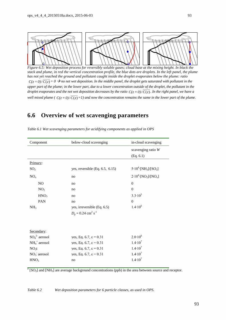
ops_v4_4_4_20150518a.docx, 2015-06-03 93

Figure 6.5: Wet deposition process for reversibly soluble gases; cloud base at the mixing height. In black the stack and plume, in red the vertical concentration profile, the blue dots are droplets. In the left panel, the plume has not yet reached the ground and pollutant caught inside the droplet evaporates below the plume: ratio

)(/ zC0)=C(z = 0 no net wet deposition. In the middle panel, the droplet gets saturated with pollutant in the upper part of the plume; in the lower part, due to a lower concentration outside of the droplet, the pollutant in the droplet evaporates and the net wet deposition decreases by the ratio )(/ zC0)=C(z . In the right panel, we have a well mixed plume ( )(/ zC0)=C(z =1) and now the concentration remains the same in the lower part of the plume.

6.6 Overview of wet scavenging parameters Table 6.1 Wet scavenging parameters for acidifying components as applied in OPS

Component below-cloud scavenging in-cloud scavenging

scavenging ratio W (Eq. 6.1)

Primary: SO2 yes, reversible (Eq. 6.5, 6.15) 5∙104∙[NH3]/[SO2]

NOx no 2∙104∙[NO2]/[NOx]

NO no 0 NO2 no 0

HNO2 no 3.3∙105 PAN no 0

NH3 yes, irreversible (Eq. 6.5) Dg = 0.24 cm2 s-1

1.4∙106

Secondary: SO4

2- aerosol yes, Eq. 6.7, ε = 0.31 2.0∙106 NH4

+ aerosol yes, Eq. 6.7, ε = 0.31 1.4∙107 NO3t yes, Eq. 6.7, ε = 0.31 1.4∙107 NO3

- aerosol yes, Eq. 6.7, ε = 0.31 1.4∙107 HNO3 no 1.4∙107

# [SO2] and [NH3] are average background concentrations (ppb) in the area between source and receptor.

Table 6.2 Wet deposition parameters for 6 particle classes, as used in OPS.

93

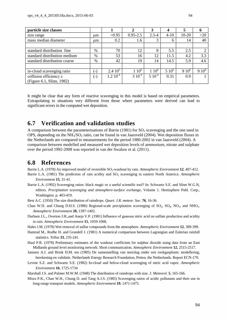
ops_v4_4_4_20150518a.docx, 2015-06-03 94

particle size classes 1 2 3 4 5 6 size range μm <0.95 0.95-2.5 2.5-4 4-10 10-20 >20 mass median diameter μm 0.2 1.6 3 6 14 40 standard distribution fine % 70 12 8 5.5 2.5 2 standard distribution medium % 53 16 12 11.5 4.2 3.3 standard distribution coarse % 42 19 14 14.5 5.9 4.6 in-cloud scavenging ratio (-) 2.4 105 1 106 1 106 5 106 9 106 9 106 collision efficiency ε (Figure 6.1, Slinn, 1982)

(-) 1.2 10-4 3 10-4 5 10-4 0.31 0.9 1

It might be clear that any form of reactive scavenging in this model is based on empirical parameters. Extrapolating to situations very different from those where parameters were derived can lead to significant errors in the computed wet deposition.

6.7 Verification and validation studies A comparison between the parameterisations of Barrie (1981) for SO2 scavenging and the one used in OPS, depending on the NH3/SO2 ratio, can be found in van Jaarsveld (2004). Wet deposition fluxes in the Netherlands are compared to measurements for the period 1980-2002 in van Jaarsveld (2004). A comparison between modelled and measured wet deposition levels of ammonium, nitrate and sulphate over the period 1992-2008 was reported in van der Swaluw et al. (2011).

6.8 References Barrie L.A. (1978) An improved model of reversible SO2-washout by rain. Atmospheric Environment 12, 407-412. Barrie L.A. (1981) The prediction of rain acidity and SO2 scavenging in eastern North America. Atmospheric

Environment 15, 31-41. Barrie L.A. (1992) Scavenging ratios: black magic or a useful scientific tool? In: Schwartz S.E. and Slinn W.G.N,

editors. Precipitation scavenging and atmosphere-surface exchange, Volume 1. Hemisphere Publ. Corp., Washington. p. 403-419.

Best A.C. (1950) The size distribution of raindrops. Quart. J.R. meteor. Soc. 76, 16-36. Chan W.H. and Chung D.H.S. (1986) Regional-scale precipitation scavenging of SO2, SO4, NO3, and NHO3.

Atmospheric Environment 20, 1397-1402. Durham J.L., Overton J.H.,and Aneja V.P. (1981) Influence of gaseous nitric acid on sulfate production and acidity

in rain. Atmospheric Environment 15, 1059-1068. Hales J.M. (1978) Wet removal of sulfur compounds from the atmosphere. Atmospheric Environment 12, 389-399. Hamrud M., Rodhe H. and Grandell J. (1981) A numerical comparison between Lagrangian and Eulerian rainfall

statistics. Tellus 33, 235-241. Haul P.R. (1978) Preliminary estimates of the washout coefficient for sulphur dioxide using data from an East

Midlands ground level monitoring network: Short communication. Atmospheric Environment 12, 2515-2517. Janssen A.J. and Brink H.M. ten (1985) De samenstelling van neerslag onder een rookgaspluim: modellering,

berekening en validatie. Netherlands Energy Research Foundation, Petten, the Netherlands. Report ECN-170. Levine S.Z. and Schwartz S.E. (1982) In-cloud and below-cloud scavenging of nitric acid vapor. Atmospheric

Environment 16, 1725-1734 Marshall J.S. and Palmer M.W.M. (1948) The distribution of raindrops with size. J. Meteorol. 5, 165-166. Misra P.K., Chan W.H., Chung D. and Tang A.J.S. (1985) Scavenging ratios of acidic pollutants and their use in

long-range transport models. Atmospheric Environment 19, 1471-1475.

94

ops_v4_4_4_20150518a.docx, 2015-06-03 95

Rodhe H. and Grandell J. (1972) On the removal time of aerosol particles from the atmosphere by precipitation scavenging. Tellus XXIV, 442-454.

Scire J.S. and Venkatram A. (1985) The contribution of in-cloud oxidation of SO2 to wet scavenging of sulfur in convective clouds. Atmospheric Environment 19, 637-650.

Seinfeld J.H. (1986) Atmospheric chemistry and physics of air pollution. John Wiley & Sons, New York. Slinn W.G.N (1982) Predictions for particle deposition to vegetative canopies. Atmospheric Environment 16, 1785-

1794. Ten Brink H.M., Janssen A.J. and Slanina J. (1988) Plume wash-out near a coal-fired power plant: measurements

and model calculations. Atmospheric Environment 22, 177-187. Van der Swaluw, Eric, Asman, Willem A.H., van Jaarsveld, Hans, Hoogerbrugge, Ronald (2011). Wet deposition

of ammonium, nitrate and sulfate in the Netherlands over the period 1992–2008, Atmospheric Environment, Volume 45, Issue 23, July 2011, Pages 3819-3826, 10.1016/j.atmosenv.2011.04.017.

Van Egmond N.D., Jaarsveld J.A. van and Onderdelinden D. (1986) The Dutch aerosol study: general overview and preliminary results. In:Lee S.D, Schneider T., Grant, L.D. and Verkerk P.J., editors. In: Aerosols: Research, Risk Assessment and Control Strategies. Lewis Publ., Chelsea, USA. p. 269-282.

Van Jaarsveld and Onderdelinden (1986): Modelmatige beschrijving van concentratie en depositie van kolen relevante componenten in NL veroorzaakt door emissies in Europa, PEO report NOK-LUK 3, RIVM report 2282 02 002, Bilthoven, the Netherlands.

Van Jaarsveld J. A. (1995) Modelling the long-term atmospheric behaviour of pollutants on various spatial scales. Ph.D. Thesis, Utrecht University, the Netherlands

Van Jaarsveld, J.A., Bleeker, A. and Hoogervorst, N.J.P. (2000) Evaluatie ammoniakredukties met behulp van metingen en modelberekeningen. RIVM rapport 722108025, RIVM, Bilthoven.

Van Jaarsveld J.A. (2004) Description and validation of OPS-Pro 4.1, RIVM report 500045001/2004.

95

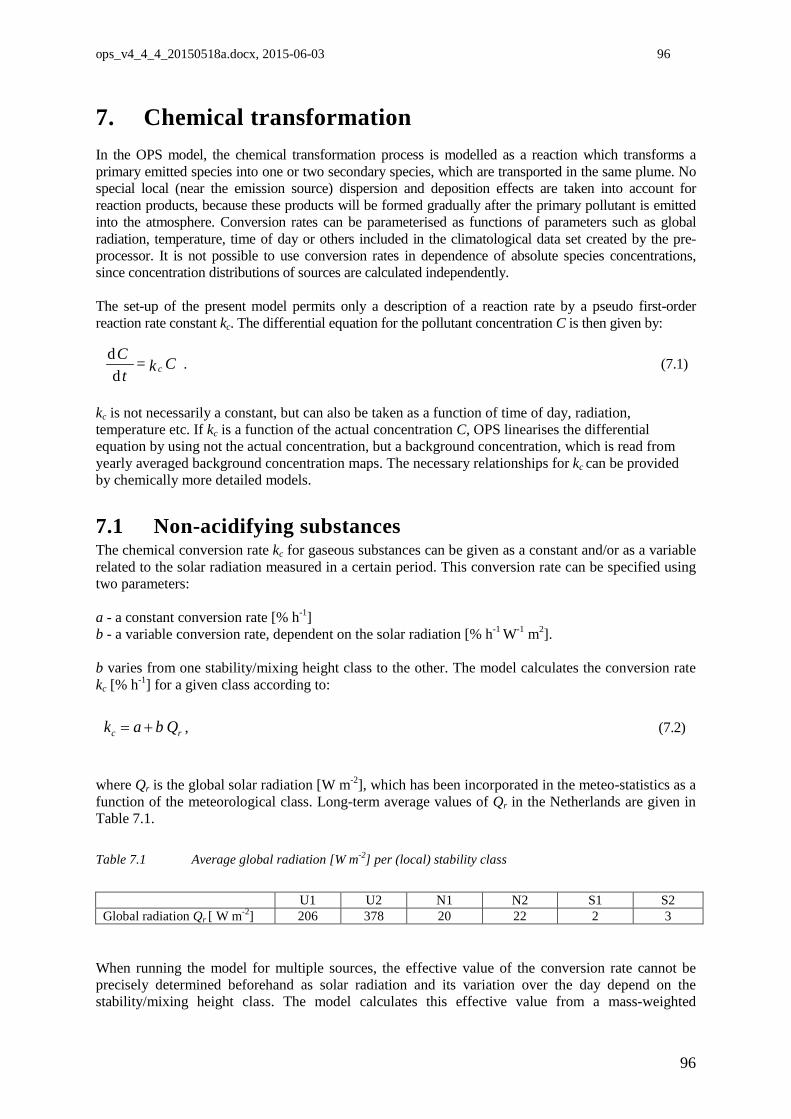
ops_v4_4_4_20150518a.docx, 2015-06-03 96

7. Chemical transformation In the OPS model, the chemical transformation process is modelled as a reaction which transforms a primary emitted species into one or two secondary species, which are transported in the same plume. No special local (near the emission source) dispersion and deposition effects are taken into account for reaction products, because these products will be formed gradually after the primary pollutant is emitted into the atmosphere. Conversion rates can be parameterised as functions of parameters such as global radiation, temperature, time of day or others included in the climatological data set created by the pre-processor. It is not possible to use conversion rates in dependence of absolute species concentrations, since concentration distributions of sources are calculated independently. The set-up of the present model permits only a description of a reaction rate by a pseudo first-order reaction rate constant kc. The differential equation for the pollutant concentration C is then given by:

kc is not necessarily a constant, but can also be taken as a function of time of day, radiation, temperature etc. If kc is a function of the actual concentration C, OPS linearises the differential equation by using not the actual concentration, but a background concentration, which is read from yearly averaged background concentration maps. The necessary relationships for kc can be provided by chemically more detailed models.

7.1 Non-acidifying substances The chemical conversion rate kc for gaseous substances can be given as a constant and/or as a variable related to the solar radiation measured in a certain period. This conversion rate can be specified using two parameters: a - a constant conversion rate [% h-1] b - a variable conversion rate, dependent on the solar radiation [% h-1 W-1 m2]. b varies from one stability/mixing height class to the other. The model calculates the conversion rate kc [% h-1] for a given class according to:

where Qr is the global solar radiation [W m-2], which has been incorporated in the meteo-statistics as a function of the meteorological class. Long-term average values of Qr in the Netherlands are given in Table 7.1. Table 7.1 Average global radiation [W m-2] per (local) stability class

U1 U2 N1 N2 S1 S2 Global radiation Qr [ W m-2] 206 378 20 22 2 3

When running the model for multiple sources, the effective value of the conversion rate cannot be precisely determined beforehand as solar radiation and its variation over the day depend on the stability/mixing height class. The model calculates this effective value from a mass-weighted

C k = t C

cdd

. (7.1)

rc Qbak += , (7.2)

96

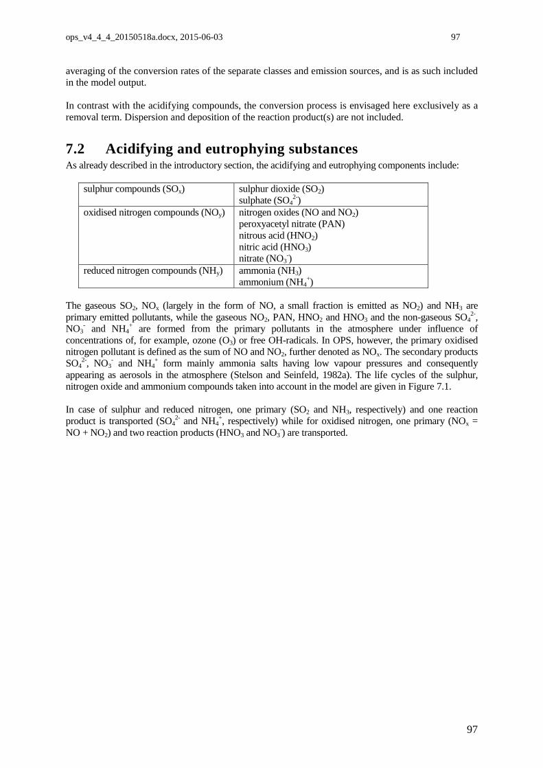
ops_v4_4_4_20150518a.docx, 2015-06-03 97

averaging of the conversion rates of the separate classes and emission sources, and is as such included in the model output. In contrast with the acidifying compounds, the conversion process is envisaged here exclusively as a removal term. Dispersion and deposition of the reaction product(s) are not included.

7.2 Acidifying and eutrophying substances As already described in the introductory section, the acidifying and eutrophying components include:

sulphur compounds (SOx) sulphur dioxide (SO2) sulphate (SO4

2-) oxidised nitrogen compounds (NOy) nitrogen oxides (NO and NO2)

peroxyacetyl nitrate (PAN) nitrous acid (HNO2) nitric acid (HNO3) nitrate (NO3

-) reduced nitrogen compounds (NHy) ammonia (NH3)

ammonium (NH4+)

The gaseous SO2, NOx (largely in the form of NO, a small fraction is emitted as NO2) and NH3 are primary emitted pollutants, while the gaseous NO2, PAN, HNO2 and HNO3 and the non-gaseous SO4

2-, NO3

- and NH4+ are formed from the primary pollutants in the atmosphere under influence of

concentrations of, for example, ozone (O3) or free OH-radicals. In OPS, however, the primary oxidised nitrogen pollutant is defined as the sum of NO and NO2, further denoted as NOx. The secondary products SO4

2-, NO3- and NH4

+ form mainly ammonia salts having low vapour pressures and consequently appearing as aerosols in the atmosphere (Stelson and Seinfeld, 1982a). The life cycles of the sulphur, nitrogen oxide and ammonium compounds taken into account in the model are given in Figure 7.1. In case of sulphur and reduced nitrogen, one primary (SO2 and NH3, respectively) and one reaction product is transported (SO4

2- and NH4+, respectively) while for oxidised nitrogen, one primary (NOx =

NO + NO2) and two reaction products (HNO3 and NO3-) are transported.

97

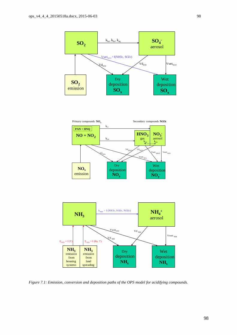
ops_v4_4_4_20150518a.docx, 2015-06-03 98

SO2SO4

-

aerosol

SO2emission

Dry deposition

SOx

Wet deposition

SOx

kho, khe, kaq

VdSO2

VwetSO 2 = f(NH3c, SO2c)

VdSO4 VwetSO 4

NH3NH4

+

aerosol

NH3emission

fromland

spreading

Dry deposition

NHx

Wet deposition

NHx

kNH3 = f (NH3c, SO2c, NO2c)

Vd NH3

Vd NH4VwetNH3

Vwet NH4

ENH3 = f (Ra, T)

NH3emission

fromhousing systems

ENH3 = f (T)

Figure 7.1: Emission, conversion and deposition paths of the OPS model for acidifying compounds.

NO + NO 2 NO 3 - aerosol

NOx emission

Dry deposition

NO y -

Wet deposition

NO y -

PAN + HNO 2 HNO 3

gas

Primary compounds NO x Secondary compounds NO3t

k OH k HN k NH

k O3

Vd NOx Vwet

NOx Vwet

NO3 Vwet HNO3

Vd HNO3 Vd NO3

98

ops_v4_4_4_20150518a.docx, 2015-06-03 99

7.2.1 Sulphur compounds Combustion of fossil fuels is the main source of atmospheric SO2 in industrialised areas. The atmospheric chemistry of sulphur can be divided into gas-phase, heterogeneous and aqueous-phase reactions. From the gas-phase reactions the most important is the oxidation by OH radicals: OH + SO2 → HOSO2 (7.3)

Prevailing evidence indicates that the HOSO2 radical ultimately leads to the formation of H2SO4, with regeneration of the OH radical (Stockwell and Calvert, 1983): HOSO2 + 2H2O → H2SO4 + OH (7.4) Heterogeneous reactions are defined here as reactions taking place within or on solid or aqueous particles other than cloud droplets. The primary process in this kind of reactions is the adsorption of SO2 by particles in which humidity plays an important role (Liberti et al., 1978). Subsequent conversion of adsorbed SO2 into sulphate depends highly on the nature of the aerosol. Using reaction chamber experiments, Haury et al. (1978) showed that SO2 oxidation is catalysed through the presence of transition metals, but that their results cannot be easily generalised and applied to atmospheric conditions. Möller (1980) suggests initial oxidation rates in industrial plumes larger than 1 x 10-5 s-1, but only a small portion of atmospheric SO2 will be oxidised in this way due to saturation of the particle surface. For the heterogeneous reactions an overall average oxidation rate of 1.7 x 10-6 s-1 is adopted here, which is 20% higher than the value suggested by De Leeuw et al. (1985). Aqueous-phase processes encompass extensive chemical transformations, many of them being oxidative in nature. In addition, there are numerous rapid equilibria in the aqueous phase. The importance of the aqueous phase transformation has been emphasised by many researchers. e.g. Möller (1980) and Lamb et al. (1987). Oxidation in cloud water by dissolved ozone (O3), hydrogen peroxide (H2O2) and by O2 catalyzed by metal ions are generally indicated as the most important mechanisms. Some authors suggest a dominating influence of NH3 (pH > 5) on the oxidation of aqueous SO2 (Stelson et al., 1979; Behra et al., 1989). This phenomenon is especially important in areas with high NH3 emissions such as the Netherlands, which means that in the present case overall conversion rates are expected to be higher than elsewhere. An average oxidation rate in water droplets was estimated by Möller (1980) at 5.0 x 10-5 s-1. A value of 4 x 10-5 s-1 is currently used in the OPS model. A suitable parameterisation of aqueous-phase processes for the present model cannot be more than a bulk parameterisation i.e. considering clouds as black boxes passing by at a certain probability with SO2 going in and sulphate aerosol coming out at a certain rate. A parameter suitable to indicating the presence of clouds would be the observed cloud cover. Since this parameter is not directly available in the meteorological data set used, the precipitation probability Pp was chosen instead. This parameter is more representative for the presence of precipitating clouds and, averaged over a longer period, might also be indicative for non-precipitating clouds. Under European conditions, most of the H2SO4 will react with NH3 to yield an NH4

+ containing aerosol. This is a one-way reaction and the aerosol will not evaporate again:

2 NH3 + H2SO4 → (NH4)2 SO4 (7.5) and

NH3 + H2SO4 → (NH4)HSO4 (7.6) These reactions form the link between sulphur and ammonia in the atmosphere.

99

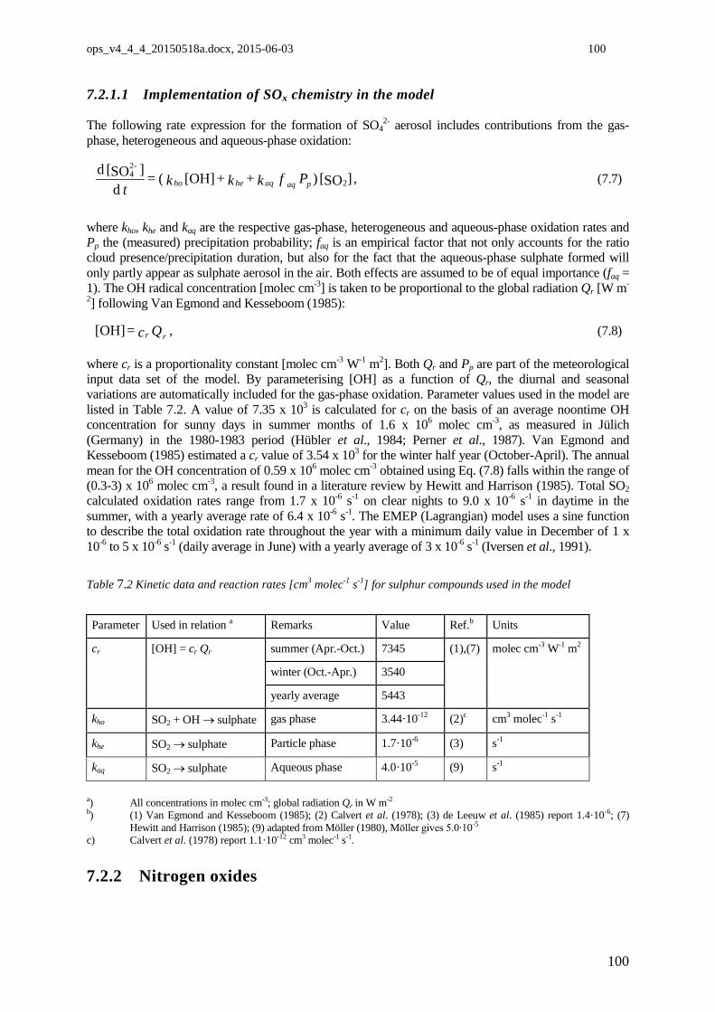
ops_v4_4_4_20150518a.docx, 2015-06-03 100

7.2.1.1 Implementation of SOx chemistry in the model The following rate expression for the formation of SO4

2- aerosol includes contributions from the gas-phase, heterogeneous and aqueous-phase oxidation:

where kho, khe and kaq are the respective gas-phase, heterogeneous and aqueous-phase oxidation rates and Pp the (measured) precipitation probability; faq is an empirical factor that not only accounts for the ratio cloud presence/precipitation duration, but also for the fact that the aqueous-phase sulphate formed will only partly appear as sulphate aerosol in the air. Both effects are assumed to be of equal importance (faq = 1). The OH radical concentration [molec cm-3] is taken to be proportional to the global radiation Qr [W m-

2] following Van Egmond and Kesseboom (1985):

where cr is a proportionality constant [molec cm-3 W-1 m2]. Both Qr and Pp are part of the meteorological input data set of the model. By parameterising [OH] as a function of Qr, the diurnal and seasonal variations are automatically included for the gas-phase oxidation. Parameter values used in the model are listed in Table 7.2. A value of 7.35 x 103 is calculated for cr on the basis of an average noontime OH concentration for sunny days in summer months of 1.6 x 106 molec cm-3, as measured in Jülich (Germany) in the 1980-1983 period (Hübler et al., 1984; Perner et al., 1987). Van Egmond and Kesseboom (1985) estimated a cr value of 3.54 x 103 for the winter half year (October-April). The annual mean for the OH concentration of 0.59 x 106 molec cm-3 obtained using Eq. (7.8) falls within the range of (0.3-3) x 106 molec cm-3, a result found in a literature review by Hewitt and Harrison (1985). Total SO2 calculated oxidation rates range from 1.7 x 10-6 s-1 on clear nights to 9.0 x 10-6 s-1 in daytime in the summer, with a yearly average rate of 6.4 x 10-6 s-1. The EMEP (Lagrangian) model uses a sine function to describe the total oxidation rate throughout the year with a minimum daily value in December of 1 x 10-6 to 5 x 10-6 s-1 (daily average in June) with a yearly average of 3 x 10-6 s-1 (Iversen et al., 1991).

Table 7.2 Kinetic data and reaction rates [cm3 molec-1 s-1] for sulphur compounds used in the model

Parameter Used in relation a Remarks Value Ref.b Units

cr [OH] = cr Qr summer (Apr.-Oct.) 7345 (1),(7)

molec cm-3 W-1 m2 winter (Oct.-Apr.) 3540

yearly average 5443

kho SO2 + OH → sulphate gas phase 3.44·10-12 (2)c cm3 molec-1 s-1

khe SO2 → sulphate Particle phase 1.7·10-6 (3) s-1

kaq SO2 → sulphate Aqueous phase 4.0·10-5 (9) s-1

a) All concentrations in molec cm-3; global radiation Qr in W m-2 b) (1) Van Egmond and Kesseboom (1985); (2) Calvert et al. (1978); (3) de Leeuw et al. (1985) report 1.4·10-6; (7)

Hewitt and Harrison (1985); (9) adapted from Möller (1980), Möller gives 5.0∙10-5 c) Calvert et al. (1978) report 1.1·10-12 cm3 molec-1 s-1.

7.2.2 Nitrogen oxides

]SO[)[OH] (d

] SO[d2

-24 P f k + k + k =

t

paqaqheho , (7.7)

Q c = rr[OH] , (7.8)

100

ops_v4_4_4_20150518a.docx, 2015-06-03 101

As stated earlier, this model was not set up to simulate complex chemistry. All relations between chemical components must be described as first-order or pseudo first-order relations. However, the structure of the model allows for easy inclusion of empirical or semi-empirical parameterisations. A brief overview of the most important reaction paths and their parameterisation follows. The relation between concentrations of NO, NO2 and O3 is to a large extent explained by the photo-stationary equilibrium:

where the equilibrium constant is proportional to the UV intensity. The reaction of NO2 with OH to form nitric acid is the main chemical loss mechanism for NO2 during daytime:

At night, NO2 is assumed to be lost by reaction with ozone to form particulate nitrate through the following series of reactions:

Hov et al. (1988) suggest that in a night-time situation the first reaction in (7.11) will be the rate-determining step. The net reaction can be written as 2 NO2 + O3 + H2O→ 2NO3

- + 2H+ + O2, with a reaction rate kO3 of 2.1 x 10-13 exp(-2450/T) cm3.molecule-1s-1. This leads to an average night-time NO2 > NO3

- conversion rate of 2.4 x 10-5 s-1. Other authors consider the hydrolysis reaction (7.11 iii) as limiting (k = 1.3 x 10-21 cm3 molec-1 s-1), leading to much lower rates. Van Egmond and Kesseboom (1983) used a first-order rate of 5.56 x 10-6 s-1 for the night-time NO2 > NO3

- conversion, the rate adopted in the OPS model. During daylight hours, the NO3 radical formed in (7.11) will be decomposed due to photolysis reactions of which NO3 + hv → NO2 + O is the most important (Magnotta and Johnston, 1980). Other (temporary) sinks for NO2 are the reaction with peroxyacetyl radicals, resulting in the formation of peroxyacetyl nitrate (PAN):

and reactions which form nitrous acid (HNO2):

The decomposition of PAN is an important function of temperature (Hov et al., 1988). Measurements in Delft carried out by TNO indicate a PAN concentration which, on average, is only in the order of 5% of the NO2 concentration (Ogilvie, 1982). The deposition properties are also uncertain but probably not very different from those of NO2; it was therefore decided not to take PAN into account as a separate component for this model but to consider it as a part of NOx.

O + NO O+ NO 223

hv↔ , (7.9)

HNO OH + NO 32 → (7.10)

.H 2 + 2NOOH + ON)(ONNO + NO)(

O + NOO + NO)(

-3(aq)252

5223

2332

+→↔→

iiiiii

(7.11)

COOCH + NO PANPAN COOCH + NO

232

232

→→

(ii) (i)

(7.12)

.NO + OH + HNOHNO + HNO OH + NO2

2

3222

→→

hv (ii) (i)

(7.13)

101

ops_v4_4_4_20150518a.docx, 2015-06-03 102

Nitrous acid (HNO2) has been studied far less extensively than for example, HNO3. The build-up of HNO2 observed during the night-time hours is still not fully explained; heterogeneous pathways have been favoured by Kessler and Platt (1984), for example. Heikes and Thompson (1983) have shown, however, that an aerosol formation mechanism is physically unlikely. The overall reaction (7.13) was postulated on results of smog chamber experiments (Cox and Jenkin, 1987; Lammel et al., 1989). Rapid photolytic decomposition takes place during the day. Slanina et al. (1990) report average HNO2 concentrations of 0.64 ppb for a forest site in the Netherlands (Speulderbos), which is in the order of 4 % of NO+NO2 concentrations. Similar results are reported by Kitto and Harrison (1992). The gaseous nitric acid may react with ammonia to form ammonium nitrate aerosol:

Temperature and relative humidity have a great influence on the equilibrium concentration of NH4NO3. Stelson and Seinfeld (1982b) indicate equilibrium constants at 80% relative humidity of 0.3 ppb2 at 10 °C and 10 ppb2 at 25 °C. Due to the relatively high ammonia concentrations in the Netherlands and other European countries, it may be expected that nitrate aerosol is the dominant form, especially in wintertime. 7.2.2.1 Implementation of NOy chemistry in the model Modelling concentrations of NO2 using the photo-stationary equilibrium reaction (7.9) requires estimates of O3 (background) concentrations on a local scale. Such O3 concentrations are strongly influenced by neighbouring NO sources, making this approach unsuited to this model. Basically, the OPS model calculates contributions of sources independent of each other, so empirical relations between NO and NO2 concentrations cannot be used unless the ‘background’ NO2 concentration is taken into account. An alternative would be an iterative approach, i.e. first calculating total concentrations linearly and then the non-linear relations using the results of the first step as the background levels. The calculated NO2, PAN and HNO2 concentrations would not be very accurate anyway. These considerations have led to the choice of modelling the sum of NO, NO2, PAN and HNO2 as a single conservative species NOx. The NO2 concentration needed in the reactions (7.10) - (7.11) is taken as a fraction of the calculated NOx concentration. Necessary NO2/NOx ratios are derived from observations as a function of atmospheric stability and trajectory length according to the classification of meteorological situations used in the model. Furthermore, the model uses maps of (prescribed) annual mean background concentrations of SO2, NO2 and NH3 as a basis for spatial and annual differences in chemistry parameterisations. Because the NOx species have rather different dry and wet deposition properties, the deposition properties of NOx are adjusted using the aforementioned NO2/NOx ratios and a (fixed) HNO2/NOx ratio. Note that modelled ‘NOx’ consist of NO + NO2 + HNO2 + PAN, including a 4% contribution of HNO2 and a possible PAN contribution of 5% to the NO2 concentration. However, measurements of NOx usually consist only of NO + NO2. At an average NO2/NOx ratio of 0.65, the modelled NOx (NO + NO2 + HNO2 + PAN) concentration may be systematically 8% higher than measured NOx (NO + NO2) concen-trations. In order to keep the model output consistent to reported concentrations, an extra 8% reduction is applied to the model output of NOx concentrations. Secondary-formed species are much less influenced by local sources. In such cases it is much less of a problem to use empirical, averaged relations between NO, NO2 and O3. The production of HNO3 for a given class s, and a transport distance x, is modelled as:

similarly to the time averaged nighttime formation of NO3

-:

)( NONH )( NH + )( HNO 3433 sgg ↔ . (7.14)

] NO [ )( ] )OH( [ = d

) HNO( dx,

3 x,srx,skt effnOH , (7.15)

102

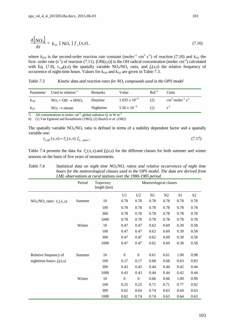
ops_v4_4_4_20150518a.docx, 2015-06-03 103

where kOH is the second-order reaction rate constant (molec-1 cm3 s-1) of reaction (7.10) and kO3 the first- order rate (s-1) of reaction (7.11). [OH(x,s)] is the OH radical concentration (molec cm-3) calculated with Eq. (7.8), rn,eff(x,s) the spatially variable NO2/NOx ratio, and fn(x,s) the relative frequency of occurrence of night-time hours. Values for kOH and kO3 are given in Table 7.3. Table 7.3 Kinetic data and reaction rates for NOy compounds used in the OPS model Parameter Used in relation a Remarks Value Ref.b Units

kOH NO2 + OH → HNO3 Daytime 1.035 x 10-11 (2) cm3 molec-1 s-1

kO3 NO2 → nitrate Nighttime 5.56 x 10 –6 (1) s-1 a) All concentrations in molec cm-3; global radiation Qr in W m-2 b) (1) Van Egmond and Kesseboom (1983); (2) Baulch et al. (1982) The spatially variable NO2/NOx ratio is defined in terms of a stability dependent factor and a spatially variable one: spacenneffn fsxrsxr _, ),(),( = . (7.17) Table 7.4 presents the data for ),( sxrn and fn(x,s) for the different classes for both summer and winter seasons on the basis of five years of measurements. Table 7.4 Statistical data on night time NO2/NOx ratios and relative occurrences of night time

hours for the meteorological classes used in the OPS model. The data are derived from LML observations at rural stations over the 1980-1985 period.

Period Trajectory length (km)

Meteorological classes

U1 U2 N1 N2 S1 S2 NO2/NOx ratio: ),( sxrn Summer 10 0.78 0.78 0.78 0.78 0.78 0.78

100 0.78 0.78 0.78 0.78 0.78 0.78 300 0.78 0.78 0.78 0.78 0.78 0.78 1000 0.78 0.78 0.78 0.78 0.78 0.78 Winter 10 0.47 0.47 0.62 0.69 0.39 0.58 100 0.47 0.47 0.62 0.69 0.39 0.58 300 0.47 0.47 0.62 0.69 0.39 0.58 1000 0.47 0.47 0.62 0.69 0.39 0.58 Relative frequency of

Summer 10 0 0 0.61 0.61 1.00 0.98

nighttime hours: fn(x,s) 100 0.17 0.17 0.68 0.68 0.63 0.83 300 0.43 0.43 0.44 0.44 0.42 0.44 1000 0.43 0.43 0.44 0.44 0.42 0.44 Winter 10 0 0 0.66 0.66 1.00 0.99 100 0.25 0.25 0.71 0.71 0.77 0.92 300 0.62 0.64 0.74 0.63 0.64 0.63 1000 0.62 0.74 0.74 0.63 0.64 0.63

[ ] )( ] NO [ = d

NO dx

-3

3x,sfkt nO , (7.16)

103

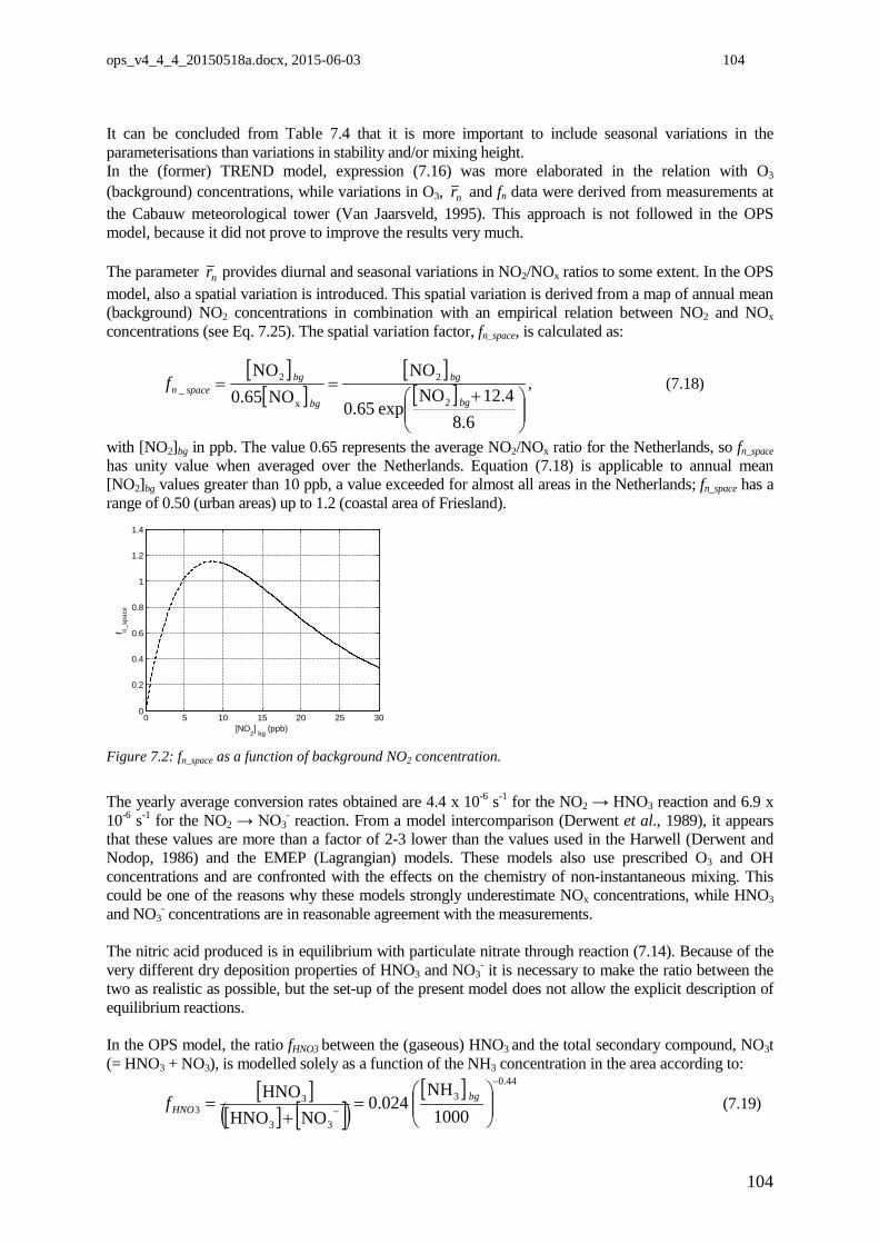
ops_v4_4_4_20150518a.docx, 2015-06-03 104

It can be concluded from Table 7.4 that it is more important to include seasonal variations in the parameterisations than variations in stability and/or mixing height. In the (former) TREND model, expression (7.16) was more elaborated in the relation with O3 (background) concentrations, while variations in O3, nr and fn data were derived from measurements at the Cabauw meteorological tower (Van Jaarsveld, 1995). This approach is not followed in the OPS model, because it did not prove to improve the results very much. The parameter nr provides diurnal and seasonal variations in NO2/NOx ratios to some extent. In the OPS model, also a spatial variation is introduced. This spatial variation is derived from a map of annual mean (background) NO2 concentrations in combination with an empirical relation between NO2 and NOx concentrations (see Eq. 7.25). The spatial variation factor, fn_space, is calculated as:

[ ][ ]

[ ][ ]

+==

6.84.12NO

exp65.0

NONO65.0

NO

2

2

x

2_

bg

bg

bg

bgspacenf , (7.18)

with [NO2]bg in ppb. The value 0.65 represents the average NO2/NOx ratio for the Netherlands, so fn_space has unity value when averaged over the Netherlands. Equation (7.18) is applicable to annual mean [NO2]bg values greater than 10 ppb, a value exceeded for almost all areas in the Netherlands; fn_space has a range of 0.50 (urban areas) up to 1.2 (coastal area of Friesland).

0 5 10 15 20 25 300

0.2

0.4

0.6

0.8

1

1.2

1.4

[NO2]

bg (ppb)

f n_sp

ace

Figure 7.2: fn_space as a function of background NO2 concentration.

The yearly average conversion rates obtained are 4.4 x 10-6 s-1 for the NO2 → HNO3 reaction and 6.9 x 10-6 s-1 for the NO2 → NO3

- reaction. From a model intercomparison (Derwent et al., 1989), it appears that these values are more than a factor of 2-3 lower than the values used in the Harwell (Derwent and Nodop, 1986) and the EMEP (Lagrangian) models. These models also use prescribed O3 and OH concentrations and are confronted with the effects on the chemistry of non-instantaneous mixing. This could be one of the reasons why these models strongly underestimate NOx concentrations, while HNO3 and NO3

- concentrations are in reasonable agreement with the measurements. The nitric acid produced is in equilibrium with particulate nitrate through reaction (7.14). Because of the very different dry deposition properties of HNO3 and NO3

- it is necessary to make the ratio between the two as realistic as possible, but the set-up of the present model does not allow the explicit description of equilibrium reactions. In the OPS model, the ratio fHNO3 between the (gaseous) HNO3 and the total secondary compound, NO3t (= HNO3 + NO3), is modelled solely as a function of the NH3 concentration in the area according to:

[ ]

[ ] [ ]( )[ ] 44.0

3

33

33 1000

NH024.0

NOHNOHNO

−

−

=

+= bg

HNOf (7.19)

104

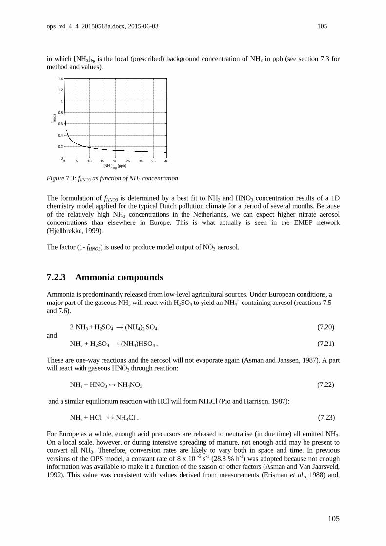
ops_v4_4_4_20150518a.docx, 2015-06-03 105

in which [NH3]bg is the local (prescribed) background concentration of NH3 in ppb (see section 7.3 for method and values).

0 5 10 15 20 25 30 35 400

0.2

0.4

0.6

0.8

1

1.2

1.4

[NH3]

bg (ppb)

f HN

O3

Figure 7.3: fHNO3 as function of NH3 concentration.

The formulation of fHNO3 is determined by a best fit to NH3 and HNO3 concentration results of a 1D chemistry model applied for the typical Dutch pollution climate for a period of several months. Because of the relatively high NH3 concentrations in the Netherlands, we can expect higher nitrate aerosol concentrations than elsewhere in Europe. This is what actually is seen in the EMEP network (Hjellbrekke, 1999). The factor (1- fHNO3) is used to produce model output of NO3

- aerosol.

7.2.3 Ammonia compounds Ammonia is predominantly released from low-level agricultural sources. Under European conditions, a major part of the gaseous NH3 will react with H2SO4 to yield an NH4

+-containing aerosol (reactions 7.5 and 7.6). 2 NH3 + H2SO4 → (NH4)2 SO4 (7.20) and NH3 + H2SO4 → (NH4)HSO4 . (7.21) These are one-way reactions and the aerosol will not evaporate again (Asman and Janssen, 1987). A part will react with gaseous HNO3 through reaction: NH3 + HNO3 ↔ NH4NO3 (7.22) and a similar equilibrium reaction with HCl will form NH4Cl (Pio and Harrison, 1987): NH3 + HCl ↔ NH4Cl . (7.23) For Europe as a whole, enough acid precursors are released to neutralise (in due time) all emitted NH3. On a local scale, however, or during intensive spreading of manure, not enough acid may be present to convert all NH3. Therefore, conversion rates are likely to vary both in space and time. In previous versions of the OPS model, a constant rate of 8 x 10 -5 s-1 (28.8 % h-1) was adopted because not enough information was available to make it a function of the season or other factors (Asman and Van Jaarsveld, 1992). This value was consistent with values derived from measurements (Erisman et al., 1988) and,

105

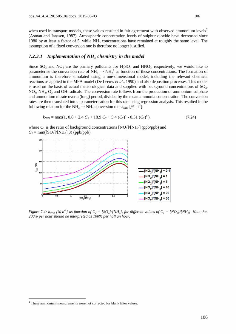
ops_v4_4_4_20150518a.docx, 2015-06-03 106

when used in transport models, these values resulted in fair agreement with observed ammonium levels2 (Asman and Janssen, 1987). Atmospheric concentration levels of sulphur dioxide have decreased since 1980 by at least a factor of 5, while NH3 concentrations have remained at roughly the same level. The assumption of a fixed conversion rate is therefore no longer justified. 7.2.3.1 Implementation of NHx chemistry in the model Since SO2 and NO2 are the primary pollutants for H2SO4 and HNO3, respectively, we would like to parameterise the conversion rate of NH3 → NH4

+ as function of these concentrations. The formation of ammonium is therefore simulated using a one-dimensional model, including the relevant chemical reactions as applied in the MPA model (De Leeuw et al., 1990) and also deposition processes. This model is used on the basis of actual meteorological data and supplied with background concentrations of SO2, NOx, NH3, O3 and OH radicals. The conversion rate follows from the production of ammonium sulphate and ammonium nitrate over a (long) period, divided by the mean ammonia concentration. The conversion rates are then translated into a parameterisation for this rate using regression analysis. This resulted in the following relation for the NH3 → NH4 conversion rate kNH3 [% h-1]: kNH3 = max(1, 0.8 + 2.4 C1 + 18.9 C2 + 5.4 (C2)4 - 0.51 (C2)6 ), (7.24) where C1 is the ratio of background concentrations [NO2]/[NH3] (ppb/ppb) and C2 = min([SO2]/[NH3],3) (ppb/ppb).

0 0.5 1 1.5 2 2.5 30

50

100

150

200

250

[SO2]/[NH3]

k NH3 [%

/h]

Figure 7.4: kNH3 [% h-1] as function of C2 = [SO2]/[NH3], for different values of C1 = [NO2]/[NH3]. Note that 200% per hour should be interpreted as 100% per half an hour.

2 These ammonium measurements were not corrected for blank filter values.

106

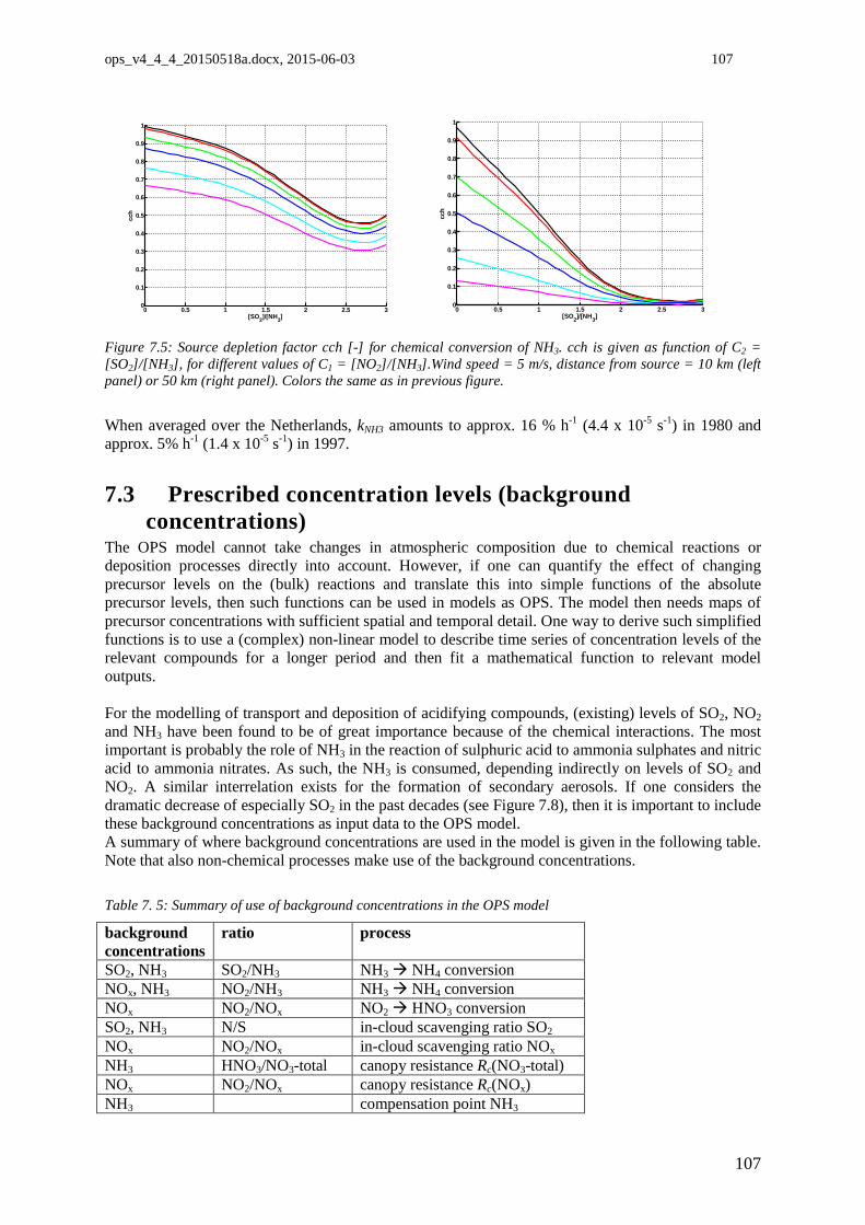
ops_v4_4_4_20150518a.docx, 2015-06-03 107

0 0.5 1 1.5 2 2.5 30

0.1

0.2

0.3

0.4

0.5

0.6

0.7

0.8

0.9

1

[SO2]/[NH3]

cch

0 0.5 1 1.5 2 2.5 30

0.1

0.2

0.3

0.4

0.5

0.6

0.7

0.8

0.9

1

[SO2]/[NH3]

cch

Figure 7.5: Source depletion factor cch [-] for chemical conversion of NH3. cch is given as function of C2 = [SO2]/[NH3], for different values of C1 = [NO2]/[NH3].Wind speed = 5 m/s, distance from source = 10 km (left panel) or 50 km (right panel). Colors the same as in previous figure.

When averaged over the Netherlands, kNH3 amounts to approx. 16 % h-1 (4.4 x 10-5 s-1) in 1980 and approx. 5% h-1 (1.4 x 10-5 s-1) in 1997.

7.3 Prescribed concentration levels (background concentrations)

The OPS model cannot take changes in atmospheric composition due to chemical reactions or deposition processes directly into account. However, if one can quantify the effect of changing precursor levels on the (bulk) reactions and translate this into simple functions of the absolute precursor levels, then such functions can be used in models as OPS. The model then needs maps of precursor concentrations with sufficient spatial and temporal detail. One way to derive such simplified functions is to use a (complex) non-linear model to describe time series of concentration levels of the relevant compounds for a longer period and then fit a mathematical function to relevant model outputs. For the modelling of transport and deposition of acidifying compounds, (existing) levels of SO2, NO2 and NH3 have been found to be of great importance because of the chemical interactions. The most important is probably the role of NH3 in the reaction of sulphuric acid to ammonia sulphates and nitric acid to ammonia nitrates. As such, the NH3 is consumed, depending indirectly on levels of SO2 and NO2. A similar interrelation exists for the formation of secondary aerosols. If one considers the dramatic decrease of especially SO2 in the past decades (see Figure 7.8), then it is important to include these background concentrations as input data to the OPS model. A summary of where background concentrations are used in the model is given in the following table. Note that also non-chemical processes make use of the background concentrations. Table 7. 5: Summary of use of background concentrations in the OPS model

background concentrations

ratio process

SO2, NH3 SO2/NH3 NH3 NH4 conversion NOx, NH3 NO2/NH3 NH3 NH4 conversion NOx NO2/NOx NO2 HNO3 conversion SO2, NH3 N/S in-cloud scavenging ratio SO2 NOx NO2/NOx in-cloud scavenging ratio NOx NH3 HNO3/NO3-total canopy resistance Rc(NO3-total) NOx NO2/NOx canopy resistance Rc(NOx) NH3 compensation point NH3

107

ops_v4_4_4_20150518a.docx, 2015-06-03 108

Background concentrations of SO2, NOx and NH3 are included as gridded maps in the OPS model. These maps encompass a large part of Western Europe and have a spatial resolution of 1 x 1 km2 for the Netherlands and 5 x 5 km2 for the foreign countries. Maps of existing concentration levels are preferably based on measurements; however, current networks are not dense enough to produce maps with sufficient detail. The method selected here is to use the OPS model in an iterative procedure, calibrating the model results with available measurements. Each iteration, OPS uses updated background concentrations of all three components; in this way, non-linearities are approximated in a stepwise linear way. The creation of background maps consists of three steps, of which step 1 and 2 are performed within this iterative procedure; the iteration stops if the iterates differ less than 0.5%. 1. Computation

Concentration maps are calculated with the OPS model for the sample years 1984, 1994, 2005, 2012 and the future year 2020, using detailed emission data.

2. Calibration

Modelled concentrations are compared with observations of the LML network and the maps are multiplied by the average ratio observed/modelled for each of the sample years.

3. Interpolation in time

For each year (starting in 1980), trend factors relative to the sample years are determined from the observations. The concentration map for a specific year is then calculated by scaling one of the sample year maps with this trend factor. The trend factor for the map of the future year is equal to 1 by definition.

Table 7.6 Representative period for each sample year for background maps sample year representative for period 1984 < 1990 1994 1990-2000 2005 2001-2006 2012 2007-X(1) 2020 (X+1)-2020 (1) X is halfway the year for which the calculation is performed and 2020

The background concentration of NO2 is derived from the background NOx concentration using a simple empirical relation derived from LML observations. This relation is:

[ ] [ ]( ) 2x12 NOlnNO ββ += , (7.25)

with [] concentrations in ppbv and empirical parameters 12.4 8.6, 21 −== ββ . This relation has been derived from 1993 LML-measurements. Since this function drops below zero for low values of [NOx],

a linear function is used for [NOx] ≤ )1exp(1

2

ββ

− , that touches the ln-function at )1exp(1

2

ββ

− and is

zero for [NOx] = 0 ppbv. This conversion function typically explains more than 90% of the variation in yearly averaged measured NO2 concentrations.

108

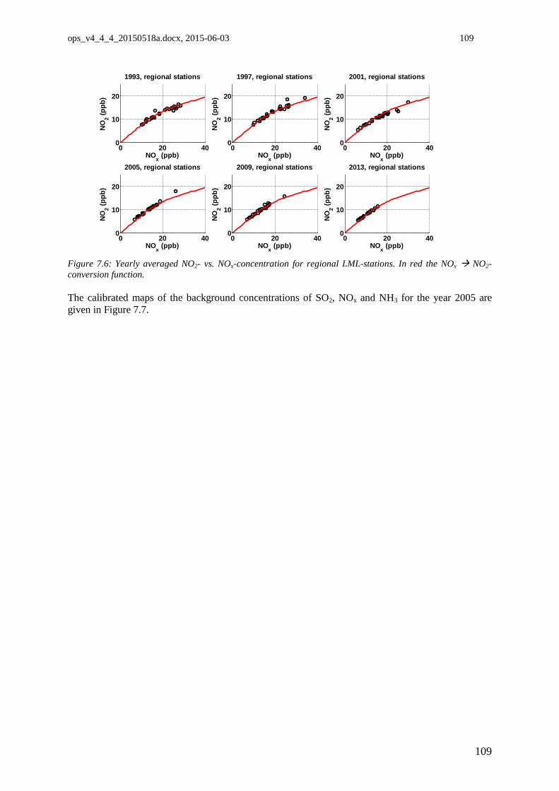
ops_v4_4_4_20150518a.docx, 2015-06-03 109

0 20 400

10

20

NOx (ppb)

NO

2 (ppb

)

1993, regional stations

0 20 400

10

20

NOx (ppb)

NO

2 (ppb

)

1997, regional stations

0 20 400

10

20

NOx (ppb)

NO

2 (ppb

)

2001, regional stations

0 20 400

10

20

NOx (ppb)

NO

2 (ppb

)

2005, regional stations

0 20 400

10

20

NOx (ppb)

NO

2 (ppb

)

2009, regional stations

0 20 400

10

20

NOx (ppb)

NO

2 (ppb

)

2013, regional stations

Figure 7.6: Yearly averaged NO2- vs. NOx-concentration for regional LML-stations. In red the NOx NO2-conversion function. The calibrated maps of the background concentrations of SO2, NOx and NH3 for the year 2005 are given in Figure 7.7.

109

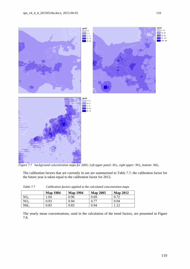
ops_v4_4_4_20150518a.docx, 2015-06-03 110

Figure 7.7 background concentration maps for 2005; Left upper panel: SO2, right upper: NOx, bottom: NH3.

The calibration factors that are currently in use are summarised in Table 7.7; the calibration factor for the future year is taken equal to the calibration factor for 2012. Table 7.7 Calibration factors applied to the calculated concentration maps

Map 1984 Map 1994 Map 2005 Map 2012 SO2 1.04 0.96 0.69 0.72 NOx 0.93 0.94 0.77 0.94 NH3 0.83 0.83 0.94 1.12 The yearly mean concentrations, used in the calculation of the trend factors, are presented in Figure 7.8.

110

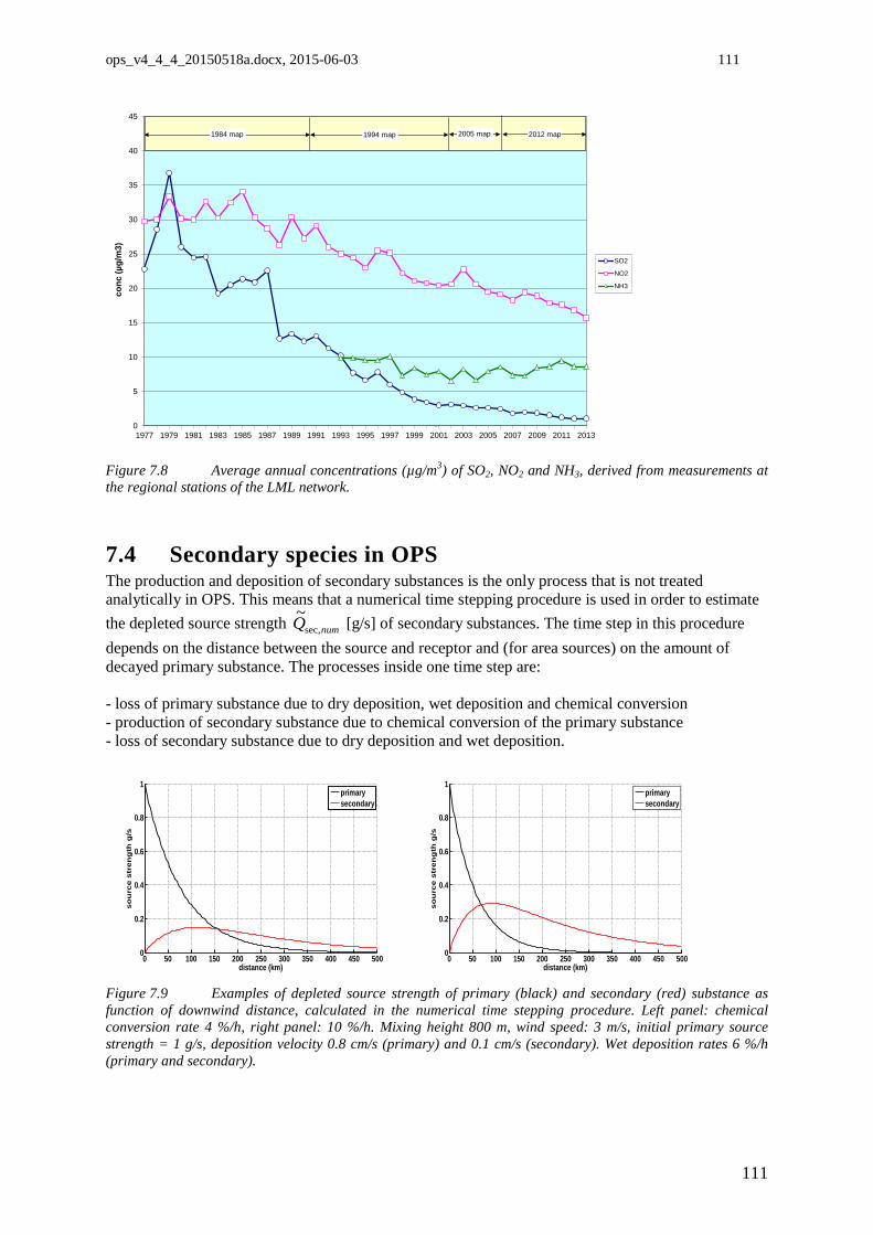
ops_v4_4_4_20150518a.docx, 2015-06-03 111

0

5

10

15

20

25

30

35

40

45

1977 1979 1981 1983 1985 1987 1989 1991 1993 1995 1997 1999 2001 2003 2005 2007 2009 2011 2013

conc

(µg/

m3)

SO2

NO2

NH3

1984 map 1994 map 2012 map2005 map

Figure 7.8 Average annual concentrations (µg/m3) of SO2, NO2 and NH3, derived from measurements at the regional stations of the LML network.

7.4 Secondary species in OPS The production and deposition of secondary substances is the only process that is not treated analytically in OPS. This means that a numerical time stepping procedure is used in order to estimate the depleted source strength numQsec,

~ [g/s] of secondary substances. The time step in this procedure depends on the distance between the source and receptor and (for area sources) on the amount of decayed primary substance. The processes inside one time step are: - loss of primary substance due to dry deposition, wet deposition and chemical conversion - production of secondary substance due to chemical conversion of the primary substance - loss of secondary substance due to dry deposition and wet deposition.

0 50 100 150 200 250 300 350 400 450 5000

0.2

0.4

0.6

0.8

1

distance (km)

so

urc

e s

tren

gth

g/s

primarysecondary

0 50 100 150 200 250 300 350 400 450 5000

0.2

0.4

0.6

0.8

1

distance (km)

so

urc

e s

tren

gth

g/s

primarysecondary

Figure 7.9 Examples of depleted source strength of primary (black) and secondary (red) substance as function of downwind distance, calculated in the numerical time stepping procedure. Left panel: chemical conversion rate 4 %/h, right panel: 10 %/h. Mixing height 800 m, wind speed: 3 m/s, initial primary source strength = 1 g/s, deposition velocity 0.8 cm/s (primary) and 0.1 cm/s (secondary). Wet deposition rates 6 %/h (primary and secondary).

111

ops_v4_4_4_20150518a.docx, 2015-06-03 112

The time stepping procedure takes place inside a sector with constant mixing height and with a constant transport velocity. To correct the source strength for this simplification, a correction is computed, based on the ratio between the analytically determined depleted source strength of the primary substance priQ~ and those of the numerical procedure numpriQ ,

~ :

numpri

prinum Q

QQQ

,sec,sec ~

~~~

= . (7.26)

Concentrations of the secondary substance are computed according to Eq. 3.7, in combination with 3.8 and 3.9 or 3.15.

7.5 References Asman W.A.H. and Janssen A.J. (1987) A long-range transport model for ammonia and ammonium for Europe.

Atmospheric Environment 21, 2099-2119. Asman W.A.H. and Jaarsveld J.A. van (1992) A variable-resolution transport model applied for NHx in Europe.

Atmospheric Environment 26A, 445-464. Baulch D.L., Cox, R.A. Crutzen P.J., Hampson R.F. Jr., Kerr, F.A. Troe, J. and Watson R.P. (1982) Evaluated

kinetic and photochemical data for atmospheric chemistry: J. Phys. Chem. Ref. Data 11 (Suppl. 1), 327-496. Behra P., Sigg L. and Stumm W. (1989) Dominating influence of NH3 on the oxidation of aqueous SO2: The

coupling of NH3 and SO2 in atmospheric water. Atmospheric Environment 23, 2691-2707. Calvert J.G., Su F., Bottenheim J.W. and Strausz O.P. (1978) Mechanism of the homogeneous oxidation of sulfur

dioxide in the troposhere. Amospheric Environment 12, 197-226. Cox R.A. and Jenkin M.E. (1987) Kinetics of the formation of nitrous acid from the thermal reaction of nitrogen

dioxide and water vapour. In: Physico-Chemical Behaviour of Atmospheric Pollutants: Proceedings of the 4th European Symposium; Stresa, Italy. D. Reidel, Dordrecht, the Netherlands.

De Leeuw F.A.A.M., Kesseboom H. and Egmond N.D. van (1985) Numerieke verspreidingsmodellen voor de interpretatie van de meetresultaten van het Nationaal Meetnet voor Luchtverontreiniging; ontwikkeling 1982-1985. RIVM, Bilthoven, the Netherlands. Report no. 842017002.

De Leeuw F.A.A.M., Rheineck Leyssius H.J. van and Builtjes P.J.H. (1990) Calculation of long term averaged ground level ozone concentrations. Atmospheric Environment 24A, 185-193.

Derwent R.G. and Nodop K. (1986) Long-range transport deposition of acidic nitrogen species in north-west Europe. Nature 324, 356-358.

Derwent R.G., Hov Ø., Asman W.A.H., Jaarsveld J.A. van and Leeuw F.A.A.M de (1989) An intercomparison of long-term atmospheric transport models; the budgets of acidifying species for the Netherlands. Atmospheric Environment 23, 1893-1909.

Erisman J.W., Vermetten A.W.M., Asman W.A.H., Waijers-IJpelaan A. and Slanina J. (1988) Vertical distribution of gases and aerosols: The vertical behaviour of ammonia and related components in the lower atmosphere. Atmospheric Environment 22, 1153-1160.

Haury G., Jordan S. and Hofmann C. (1978) Experimental investigation of the aerosol-catalyzed oxidation of SO2 under atmospheric conditions. Atmospheric Environment 12, 281-287.

Heikes B.G. and Thompson A.M. (1983) Effects of heterogeneous processes on NO3, HONO and HNO3 chemistry in the troposphere. J. Geophys. Res. 88, 10883-10895.

Hewitt C.N. and Harrison R.M. (1985) Tropospheric concentrations of the hydroxyl radical - A review. Atmospheric Environment 19, 545-554.

Hjellbrekke A.G. (1999) Data Report 1997; Part 1: Annual summaries. EMEP/CCC-Report 3/99, Norwegian Institute for Air Research, Kjeller, Norway.

Hov Ø., Eliassen A. and Simpson D. (1988) Calculation of distribution of NOx compounds in Europe. In: Isaksen I.S.A., editor. Tropospheric Ozone. D. Reidel, Dordrecht, the Netherlands. p. 239-261.

Hübler G. Perner D., Platt U., Tönnissen A. and Ehhalt D.H. (1984) Groundlevel OH radical concentration: New measurements by optical absorption. J. Geophys. Res. 89, 1309-1320.

112

ops_v4_4_4_20150518a.docx, 2015-06-03 113

Iversen T., Halvorsen N.E., Mylona S. and Sandnes H. (1991) Calculated budgets for airborne acidifying components in Europe; 1985,1987,1988,1989 and 1990. The Norwegian Meteorological Institute, Oslo, Norway. EMEP/MSC-W Report 1/91.

Kessler C. and Platt U. (1984) Nitrous acid in polluted air masses: sources and formation pathways. In: Versino, B. and Angeletti, editors. Physico-Chemical Behaviour of Atmospheric Pollutants. Proceedings of the European symposium; Varese, Italy. D. Reidel, Dordrecht, the Netherlands.

Kitto A.M.N. and Harrison R.M. (1992) Nitrous and nitric acid measurements at sites in south-east England. Atmospheric Environment 26A, 235-241.

Lamb D. Miller D.F., Robinson N.F. and Gertler A.W. (1987) The importance of liquid water concentration in the atmospheric oxidation of SO2. Atmospheric Environment 21, 2333-2344.

Lammel G., Perner D. and Warneck P. (1989) Nitrous acid at Mainz: observation and implication for its formation mechanism. In: Restelli G. and Angeletti G., editors. Physico-Chemical Behaviour of Atmospheric Pollutants: Proceedings of the 5th European symposium; Varese, Italy. D. Reidel, Dordrecht, the Netherlands.

Liberti A. Brocco D. and Possanzini M. (1978) Absorption and oxidation of sulfur dioxide on particles. Atmospheric Environment 12, 255-261

Magnotta F. and Johnston H.S. (1980) Photodissociation quantum yields for the NO3 free radical. Geophys. Res. Lett. 7, 769-772.

Möller D. (1980) Kinetic model of atmospheric SO2 oxidation based on published data. Atmospheric Environment 14, 1067-1076.

Ogilvie F.R. (1982) Buitenluchtverontreiniging in Delft in 1980. TNO, Delft, the Netherlands. Report G 980. Perner D., Platt U., Trainer M., Hübler G., Drummond J., Junkermann W., Rudolph J., Schubert B. and Ehhalt

D.H. (1987) Measurements of tropospheric OH concentrations: A comparison of field data with model predictions. J. Atmos. Chem. 5, 185-216.

Pio C.A. and Harrison R.M. (1987) The equilibrium of ammonium chloride aerosol with gaseous hydrochloric acid and ammonia under tropospheric conditions. Atmospheric Environment 21, 1243-1246.

Slanina J., Keuken M.P., Arends B., Veltkamp A.C. and Wyers G.P. (1990) Acidification research at ECN. Contribution to the Dutch Priority Programme on Acidification. ECN, Petten, the Netherlands.

Stelson A.W., Friedlander S.K. and Seinfeld J.H. (1979) A note on the equilibrium relation ship between ammonia and nitric acid and particulate ammonium nitrate. Atmospheric Environment 13, 369-371.

Stelson A.W. and Seinfeld J.H. (1982a) Relative humidity and pH dependence of the vapor pressure of ammonium nitrate-nitric acid solutions at 25 oC. Atmospheric Environment 16, 993-1000.

Stelson A.W. and Seinfeld J.H. (1982b) Relative humidity and temperature dependence of ammonium nitrate dissociation constant. Atmospheric Environment 16, 983-992.

Stockwell W.R. and Calvert J.G. (1983) The mechanism of the HO-SO2 reaction. Atmospheric Environment 17, 2231-2235.

Van Egmond N.D. and Kesseboom H. (1983) Mesoscale air pollution dispersion models-II. Lagrangian PUFF-model, and comparison with Eulerian GRID model. Atmospheric Environment, 17, 265-274.

Van Egmond N.D. and Kesseboom H. (1985) A numerical mesoscale model for long- term average NOx and NO2-concentration. Atmospheric Environment 19, 587- 595.

Van Jaarsveld J. A. (1995) Modelling the long-term atmospheric behaviour of pollutants on various spatial scales. Ph.D. Thesis, Utrecht University, the Netherlands.

Van Jaarsveld, J.A., Bleeker, A. and Hoogervorst, N.J.P. (2000) Evaluatie ammoniakredukties met behulp van metingen en modelberekeningen. RIVM, Bilthoven, the Netherlands. Report no. 722108025.

113