THE NON-CENTRAL χ2-LAW

IN FINANCE: A SURVEY

Jan-Frederik MaiXAIA Investment GmbHSonnenstraße 19, 80331 München, Germanyjan-frederik.mai@xaia.com

First Version: April 28, 2014

This Version: April 20, 2015

Abstract The non-central χ2-distribution appears in various financial appli-cations. The present article surveys the key features to be knownabout this distribution, reviews some numerical techniques invol-ved in its implementation, and collects a number of examples forits use in the context of Mathematical Finance. The article is or-ganized as follows: Section 1 defines the non-central χ2-law andreviews its key features. Section 2 defines squared Bessel pro-cesses, which might be viewed as dynamic counterparts of thestatic non-central χ2-distribution, and surveys their key features.Finally, Section 3 briefly outlines some of the financial applicati-ons involving the non-central χ2-distribution, and Section 4 con-cludes.

1 Static viewpoint: the non-central

χ2-distribution

Throughout, we denote by

||x|| :=√x2

1 + . . .+ x2δ , x = (x1, . . . , xδ) ∈ Rδ

the Euclidean norm on Rδ. If Z is multivariate normal in dimen-sion δ ∈ N with mean vector µ ∈ Rδ and the identity matrixas covariance matrix, then the random variable Y := ||Z||2 issaid to have a non-central χ2-law with non-centrality parameterα := ||µ||2 ≥ 0 and δ degrees of freedom. This is the most com-mon and most intuitive introduction of the non-central χ2-law. Inparticular, if α = 0, one is left with the regular χ2-distributionwith δ ∈ N degrees of freedom, which is well-known from ele-mentary statistics lectures. For many applications in Mathema-tical Finance it is reasonable to generalize the definition also tonon-integer degrees of freedom δ > 0. This is formally accom-plished in the following definition.

Definition 1.1 (The non-central χ2-distribution)A positive random variable Y is said to follow the non-centralχ2-distribution with δ > 0 degrees of freedom and non-centralityparameter α > 0, denoted Y ∼ χ2(δ, α), if its density is given by

fχ2(δ,α)(x) :=1

2e−

α+x2

(xα

) δ4− 1

2I δ

2−1

(√αx), x > 0,

where Iν denotes the modified Bessel function of the first kindwith index ν, given by the series representation

Iν(x) =

∞∑n=0

1

n! Γ(ν + n+ 1)

(x2

)ν+2n, x > 0.

111

An efficient evaluation of the function Iν(x) for real ν and non-negative x, as required, is standard. For instance, in MATLABit is pre-implemented in the routine besseli. Consequently, thedensity of the non-central χ2-distribution is given in a numericallyconvenient closed form.

1.1 Laplace transform A straightforward computation shows that the Laplace transformof Y ∼ χ2(δ, α) is given by

E[e−uY

]=

1

(1 + 2u)δ2

e−αu

1+2u =: e−Ψ(u), u ≥ 0,

Ψ(u) =δ

2log(1 + 2u) +

αu

1 + 2u, u ≥ 0. (1)

The same computation (with u = 0) indeed also verifies thatfχ2(δ,α) is a proper density. The function Ψ : [0,∞) → [0,∞)is a so-called complete Bernstein function, see Schilling et al.(2010) for detailed information on these functions. This impliesthat the non-central χ2-law is infinitely divisible, and even more,it is part of the so-called Bondesson family of distributions, whichwas introduced in Bondesson (1981) under the name g.c.m.e.d.distributions, see also Bondesson (1979). The latter distributionsarise, e.g., as the laws of first hitting times of diffusion processesand have very convenient properties, see Schilling et al. (2010)for details. Moreover, we observe that Ψ = Ψ1 + Ψ2, where

Ψ1(u) =δ

2log(1 + 2u), Ψ2(u) =

αu

1 + 2u, u ≥ 0,

are also two complete Bernstein functions. The Bernstein functi-on Ψ1 corresponds to a Γ-distribution Γ(δ/2, 1/2), using the pa-rameterization of (Mai, Scherer, 2012, p. 2). The Bernstein func-tion Ψ2 corresponds to a compound Poisson sum (the Poissoncounting variable has mean α/2) of exponentially distributed ran-dom variables with mean 2.

Remark 1.2 (Zero degrees of freedom)The function Ψ is clearly also a complete Bernstein function inthe case δ = 0 (pure compound Poisson case). Hence, it makessense to define the non-central χ2-law for all δ ≥ 0, but for δ = 0it has no density, because it has an atom at zero.

1.2 Mixture representation It is readily observed that

fχ2(δ,α)(x) =

∞∑n=0

e−α2

n!

(α2

)nfΓ(δ/2+n,1/2)(x), x > 0, (2)

where fΓ(β,η) denotes the density of a Γ-distribution with para-meters β, η, again using the parameterization of (Mai, Scherer,2012, p. 2). This shows that the non-central χ2-distribution maybe viewed as the Poisson mixture of Gamma distributions. Con-cerning a stochastic representation, it follows from the aforemen-tioned decomposition of Ψ into Ψ1 and Ψ2 that

Y := G+N∑k=1

Jk ∼ χ2(δ, α), (3)

222

where1 G ∼ Γ(δ/2, 1/2), N ∼ Poi(α/2) and J1, J2, . . . ∼ E(1/2)are stochastically independent. This stochastic representationimplies a quick simulation algorithm for χ2(δ, α), provided simula-tion algorithms for the involved Gamma-, Poisson-, and exponen-tial distribution are given. For the latter, see (Mai, Scherer, 2012,Chapter 6). Recalling the well-known fact that Γ(δ/2, 1/2)+Γ(N, 1/2) =Γ(δ/2 + N, 1/2), this is in line with the Poisson mixture repre-sentation (2) of the density, respectively an alternative derivationthereof. Alternatively, one might also re-write the sum in (3) as astopped Gamma subordinator2:

N∑k=1

Jkd= ΛN ,

where Λ = Λtt≥0 is a Gamma subordinator3, independent ofN ∼ Poi(α/2), with parameters (1, 1/2), using the parameteri-zation of (Mai, Scherer, 2012, p. 274).

1.3 Distribution function Starting from the representation (2), the distribution function is aPoisson mixture of certain Gamma distributions. Benton, Kris-hnamoorthy (2003) propose an algorithm to compute this se-ries efficiently4. Alternatively5, we present a way of computingthe distribution function based on (Bernhart et al., 2014, Corol-lary 3.4). This method to compute the distribution function re-lies on Laplace inversion, i.e. the distribution function is retrie-ved from its known Laplace transform. It is applicable in the pre-sent situation, since the non-central χ2-distribution is part of theBondesson class, for which Bernhart et al. (2014) is known towork. If we denote the distribution function of Y ∼ χ2(δ, α) byFχ2(δ,α), (Bernhart et al., 2014, Corollary 3.4) implies for x > 0that Fχ2(δ,α)(x) =

M

π

∫ 1

0Im

(ex a−xM log(v) (b i−a)−Ψ

(a−M log(v) (b i−a)

)a/(b i− a)−M log(v)

)dv

v, (4)

for arbitrary a, b > 0 and M > 2/(a x). The integrand vanishesas v 0, i.e. the integral is a proper Riemann integral. In parti-cular, choosing a = b = 1/x, and M > 2 arbitrary, the integrandin (4) can be bounded from above by a constant independent ofx and δ as follows:∣∣∣∣∣Im

(ex a−xM log(v) (b i−a)−Ψ

(a−M log(v) (b i−a)

)a/(b i− a)−M log(v)

)∣∣∣∣∣ ≤ 2 vM e1+α4 .

1We denote by Poi(λ) and E(λ) the Poisson- and exponential distribution withrate parameter λ > 0.

2We denote by d= equality in distribution.

3Recall that a Gamma subordinator λtt≥0 with parameters (β, η) is a non-decreasing stochastic process with Λ0 = 0, independent and stationaryΓ(t β, η)-distributed increments Λt+s − Λs, 0 ≤ s < t.

4See also Dalgaard (2001) and the references cited in Benton, Krishnamoor-thy (2003) for related literature.

5The Laplace inversion formula (4) agrees with the method described by Ben-ton, Krishnamoorthy (2003), which is also pre-implemented in MATLAB asncx2cdf, up to an accuracy of about 10−12. We tested several sets of pa-rameters α, δ.

333

Interestingly, there exists also a quick-and-dirty approximation forthe distribution function, which might be useful for an approxima-tive implementation on an EXCEL spreadsheet. It is derived inSankaran (1959) and states for x ≥ 0 that Fχ2(δ,α)(x) ≈

Φ

((x

α+δ

)hδ,α− (1 + hδ,α pδ,α (hδ,α − 1− (2−hδ,α)mδ,α pδ,α2 )

)hδ,α

√2 pδ,α (1 +mδ,α pδ,α/2)

),

(5)

where Φ denotes the standard normal cdf and

hδ,α = 1− 2 (δ + α) (δ + 3α)

3 (δ + 2α)2, pδ,α =

δ + 2α

(δ + α)2,

mδ,α = (hδ,α − 1) (1− 3hδ,α).

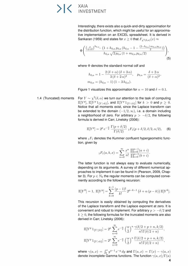
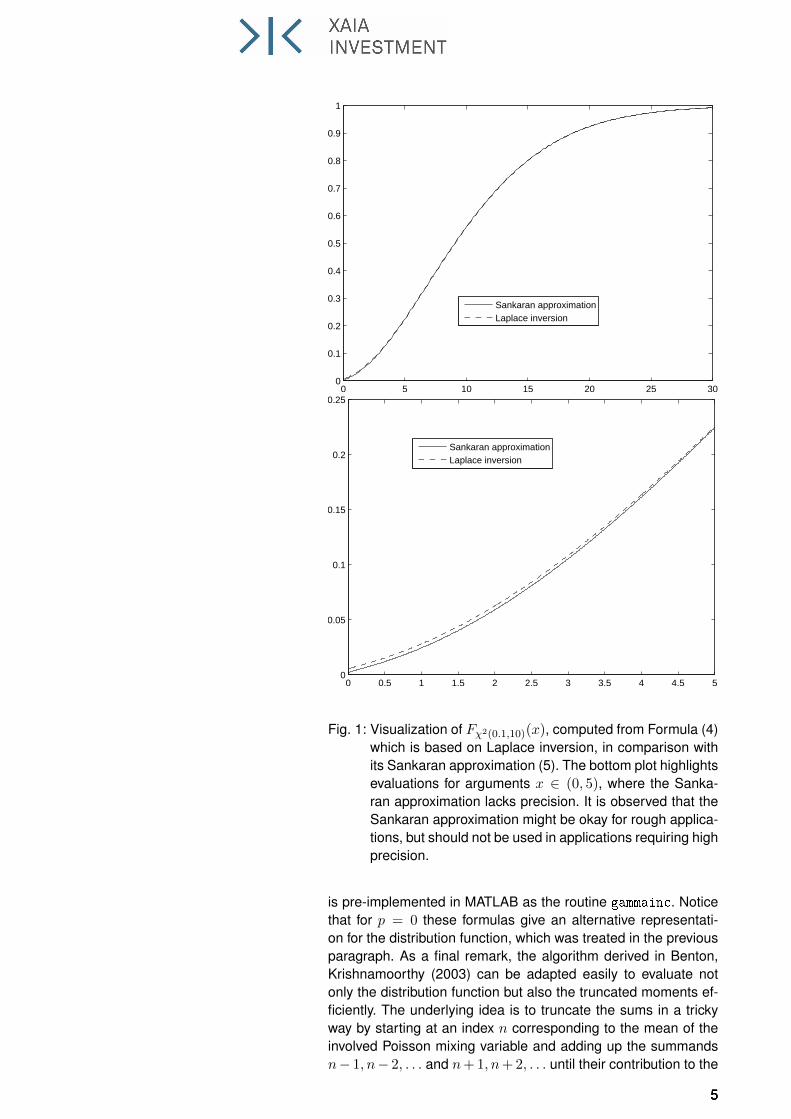
Figure 1 visualizes this approximation for α = 10 and δ = 0.1.

1.4 (Truncated) moments For Y ∼ χ2(δ, α) we turn our attention to the task of computingE[Y p], E[Y p 1Y >k], and E[Y p 1Y <k] for k > 0 and p ≥ 0.Notice that all moments exist, since the Laplace transform canbe extended to the domain (−1/2,∞), i.e. a domain includinga neighborhood of zero. For arbitrary p > −δ/2, the followingformula is derived in Carr, Linetsky (2006):

E[Y p] = 2p e−α2

Γ(p+ δ/2)

Γ(δ/2)1F1(p+ δ/2, δ/2, α/2), (6)

where 1F1 denotes the Kummer confluent hypergeometric func-tion, given by

1F1(a, b, x) =∞∑n=0

xn

n!

∏n−1i=0 (a+ i)∏n−1i=0 (b+ i)

.

The latter function is not always easy to evaluate numerically,depending on its arguments. A survey of different numerical ap-proaches to implement it can be found in (Pearson, 2009, Chap-ter 3). For p ∈ N0 the regular moments can be computed conve-niently according to the following recursion:

E[Y 0] = 1, E[Y p] =

p−1∑k=0

(p− 1)!

k!2p−k−1

(δ + α (p− k)

)E[Y k].

This recursion is easily obtained by computing the derivativesof the Laplace transform and the Laplace exponent at zero. It isconvenient and robust to implement. For arbitrary p > −δ/2 andk ≥ 0, the following formulas for the truncated moments are alsoderived in Carr, Linetsky (2006):

E[Y p 1Y≤k] = 2p∞∑n=0

e−α2

(α2

)n γ(δ/2 + p+ n, k/2)

n! Γ(δ/2 + n),

E[Y p 1Y >k] = 2p∞∑n=0

e−α2

(α2

)n Γ(δ/2 + p+ n, k/2)

n! Γ(δ/2 + n),

where γ(a, x) =∫ x

0 ya−1 e−y dy and Γ(a, x) = Γ(x) − γ(a, x)

denote incomplete Gamma functions. The function γ(a, x)/Γ(a)

444

0 5 10 15 20 25 300

0.1

0.2

0.3

0.4

0.5

0.6

0.7

0.8

0.9

1

Sankaran approximationLaplace inversion

0 0.5 1 1.5 2 2.5 3 3.5 4 4.5 50

0.05

0.1

0.15

0.2

0.25

Sankaran approximationLaplace inversion

Fig. 1: Visualization of Fχ2(0.1,10)(x), computed from Formula (4)which is based on Laplace inversion, in comparison withits Sankaran approximation (5). The bottom plot highlightsevaluations for arguments x ∈ (0, 5), where the Sanka-ran approximation lacks precision. It is observed that theSankaran approximation might be okay for rough applica-tions, but should not be used in applications requiring highprecision.

is pre-implemented in MATLAB as the routine gammainc. Noticethat for p = 0 these formulas give an alternative representati-on for the distribution function, which was treated in the previousparagraph. As a final remark, the algorithm derived in Benton,Krishnamoorthy (2003) can be adapted easily to evaluate notonly the distribution function but also the truncated moments ef-ficiently. The underlying idea is to truncate the sums in a trickyway by starting at an index n corresponding to the mean of theinvolved Poisson mixing variable and adding up the summandsn− 1, n− 2, . . . and n+ 1, n+ 2, . . . until their contribution to the

555

overall sum becomes negligible.

2 Dynamic viewpoint: squared

Bessel processes

The non-central χ2-distribution arises as the marginal law of so-called squared Bessel processes. In this sense, squared Besselprocesses may be viewed as a dynamic counterpart to the non-central χ2-distribution, just like Brownian motion is a dynamiccounterpart of the standard normal distribution. In MathematicalFinance there are many applications involving squared Besselprocesses, and hence implicitly the non-central χ2-distribution.Therefore, we collect some useful background information regar-ding Bessel processes in the present section. To this end, wedenote by W = Wt standard Brownian motion.

Definition 2.1 ((Squared) Bessel process)(a) A diffusion process Xt is called a Bessel process with in-

dex ν ∈ R if it follows the stochastic differential equation

dXt =2 ν + 1

2Xtdt+ dWt.

(b) A diffusion process Yt is called squared Bessel process ofdimension δ if there exists a Bessel process Xt of index

ν = (δ − 2)/2 such that Ytd= X2

t , or equivalently, if itfollows the stochastic differential equation

dYt = δ dt+ 2√|Yt| dWt.

Notice in particular that the absolute value under the squareroot in the defining stochastic differential equation of the squaredBessel process may be dropped a posteriori in the case δ ≥ 0,because Yt ≥ 0 almost surely in this case, see Subsection 2.2below.

2.1 Existence of (squared) Besselprocesses

If δ := 2 ν+ 2 ∈ 2, 3, 4, . . . is a natural number ≥ 2, then it canbe shown using Itô calculus that Xt := ||µ + W

(δ)t ||, t ≥ 0, is

a Bessel process with index ν, where W (δ)t denotes standard,

δ-dimensional Brownian motion, and µ ∈ Rδ. Hence, in this casea squared Bessel process of dimension δ exists, namely Yt :=

X2t = ||µ+W

(δ)t ||2, t ≥ 0. For t > 0 we observe

Ytt

=∣∣∣∣∣∣ µ√

t+W

(δ)t√t

∣∣∣∣∣∣2d=∣∣∣∣∣∣ µ√

t+W

(δ)1

∣∣∣∣∣∣2 ∼ χ2(δ,||µ||2

t

)= χ2

(δ,X2

0

t

).

It follows that the Markov transition kernel of the squared Besselprocess of dimension δ, i.e. the conditional density of Ys+t givenYs = x for arbitrary s ≥ 0, is given by

pt(x, y) :=1

tfχ2(δ,x/t)

(yt

), t, x, y > 0.

Considering the Markov transition kernel for δ ∈ 2, 3, 4, . . .,one may define an analytical extension of it to arbitrary degreesof freedom δ ≥ 0, just like the non-central χ2-law is extendedanalytically to δ ≥ 0. With a Kolmogorov existence argument it

666

can be shown that a squared Bessel process of arbitrary dimen-sion δ ≥ 0 exists. Hence, a Bessel process of arbitrary indexν ≥ −1 exists and is defined as the square root of the squa-red Bessel process constructed in this way. It is further explai-ned in, e.g., Göing-Jaeschke, Yor (2003) that Bessel processeswith arbitrary real index ν ∈ R and squared Bessel processesof arbitrary dimension δ ∈ R exist as well, i.e. the defining sto-chastic differential equations admit unique solutions, which areadapted to the filtration of the driving Brownian motion (so-calledstrong solution). Squared Bessel processes with negative indexthat start at a positive value almost surely hit zero in finite time.After that they become negative and behave similar to the nega-tive of a squared Bessel process with positive index.

2.2 Hitting times of zero The following can be shown6 for a squared Bessel process Y =Yt of dimension δ ≥ 0 which starts at a positive value Y0 > 0,which of course translates into analogous statements for Besselprocesses with index ν := (δ − 2)/2 ≥ −1:

• δ = 0: The process Y hits zero almost surely in finite time,and remains there.

• 0 < δ < 2: The process Y hits zero infinitely many times andlim supt→∞ Yt =∞.

• δ = 2: The process Y is strictly positive with lim inft→∞

Yt = 0

and lim supt→∞ Yt =∞.

• δ > 2: The process Y is strictly positive with limt→∞ Yt =∞.

Notice in particular that these statements contain the well-knownfact that the origin (or any other point) is recurrent for one- andtwo-dimensional Brownian motion, whereas it is transient in lar-ger dimensions. It is further easy to see from the Laplace trans-form of the non-central χ2-law that for δ = 0 we have

P(Yt = 0) = limu→∞

E[e−uYt

]= lim

u→∞e−

Y0 u1+2u t = e−

Y02 t , t > 0.

2.3 Further useful properties One immediately checks that a squared Bessel process Y =

Yt satisfies the scaling property Ytd= Yc t/c for each c >

0. Another key feature is the additivity property, stating that thesum of independent squared Bessel processes of non-negativedimensions δ1, δ2 ≥ 0 is again a squared Bessel process of di-mension δ1 + δ2, see Shiga, Watanabe (1973). Moreover, one ofthe most useful identities regarding Bessel processes relates itslaw to the distribution of a Bessel process with index zero. This isespecially useful when dealing with Bessel processes with nega-tive index (which might diffuse to zero), because it allows to trans-form the analysis to a Bessel process which cannot diffuse tozero. Recall from Subsection 2.2 that a Bessel process remainsalmost surely positive whenever its index ν is non-negative. Thefollowing lemma is stated and massively used in Yor (1992).

6See, e.g., http://almostsure.wordpress.com/2010/07/28/bessel-processes/.

777

Lemma 2.2 (Useful transformation of Bessel index)On a filtered probability space (Ω,F ,P, Ft) supporting a stan-dard Brownian motion Wt with natural filtration Ft, deno-te the Bessel process with index ν ∈ R by X(ν) = X(ν)

t ,and its first hitting time of zero by Tν ∈ (0,∞]. Moreover, wedenote by X(0) = X(0)

t the Bessel process with index zeroand X

(0)0 = X

(ν)0 > 0. For all bounded, continuous functions

f : R→ R and t > 0 it holds that

E[f(X

(ν)t

)1Tν>t

]= E

[f(X

(0)t

)(X(0)t

X(0)0

)νe− ν

2

2

∫ t0

1

X(0)s

ds].

Remark 2.3 (Bessel processes and Asian options)Lemma 2.2 is used in Yor (1992) in order to derive the densi-ty of the integral over geometric Brownian motion, which playsa dominant role in Asian option pricing within a Black-Scholescosmos. The reference Carr, Schröder (2004) further explains inquite some detail how Bessel processes play a dominant role inthis context.

3 Applications in Mathematical

Finance

The popularity of the non-central χ2-distribution in MathematicalFinance stems from its involvement in two quite popular models:the CEV stock price model and the CIR model. The underlyingstochastic processes in both models can be viewed as certaintransformations of squared Bessel processes, indicating how thenon-central χ2-distribution comes into play.

3.1 The CEV model The constant elasticity of variance (CEV) model defines the priceprocess Stt≥0 of an asset as a diffusion process satisfying thestochastic differential equation

dSt = µSt dt+ σ Sρt dWt, (7)

where the parameter ρ ≥ 0 controls the relation between leveland volatility of the price process. For ρ < 1, the volatility incre-ases with a decreasing asset price (leverage effect), whereas itincreases with an increasing asset price for ρ > 1 (inverse le-verage effect). For ρ = 1, the model boils down to the standardBlack-Scholes model with volatility σ > 0 and drift µ ∈ R. Inthe leverage effect case ρ ∈ (0, 1) and for non-negative µ ≥ 0,the reference Delbaen, Shirakawa (2002) interprets S as a stockprice process and uses Lemma 2.2 in order to show that the pro-cess Stt≥0, given by

St := eµ t

(Y

(δρ)

minTδρ ,σ2 (1−ρ)

2µ

(1−e−2µ (1−ρ) t

)

) 12−2 ρ

,

satisfies (7), where δρ := (1 − 2 ρ)/(1 − ρ) ∈ (−∞, 1), Y (δρ) =

Y (δρ)t t≥0 is a squared Bessel process of dimension δρ starting

at Y (δρ)0 = S2−2 ρ

0 , and Tδρ ∈ (0,∞] its first hitting time of zero.This stochastic representation of the CEV process in terms of asquared Bessel process allows to derive its probability distributi-on in terms of the non-central χ2-distribution:

888

• For non-negative x ≥ 0 it follows with the help of Lemma 2.2that P(St > x) =

Fχ2

(1

1−ρ ,2µ (e−µ t x)2 (1−ρ)

σ2 (1−ρ) (1−e−2µ (1−ρ) t)

)( 2µS2 (1−ρ)0

σ2 (1− ρ)(1− e−2µ (1−ρ) t

)).Notice that the formula is well-defined also for µ = 0 as therespective limit for µ 0 exists.

• There is a positive probability that the asset price diffusesto zero and remains there. However, there is also a positiveprobability that the asset price never touches zero. The pro-bability that the asset price equals zero at time t > 0 is givenby

P(St = 0) = P(Tδρ <

σ2 (1− ρ)

2µ

(1− e−2µ (1−ρ) t

))= 1− F

χ2(

11−ρ ,0

)( 2µS2 (1−ρ)0

σ2 (1− ρ)(1− e−2µ (1−ρ) t

)).Notice that the formula is well-defined also for µ = 0 as therespective limit for µ 0 exists. Notice further that the li-mit as t → ∞ of the last expression gives the probabilitythat the asset price becomes zero at all, because the eventsSt = 0 are decreasing in t (hitting zero once, the asset pri-ce remains there). Hence, there is also a positive probabilitythat the stock price never touches zero, given by

P(St > 0 for all t > 0) = Fχ2(

11−ρ ,0

)(2µS2 (1−ρ)0

σ2 (1− ρ)

).

Because of the positive probability that the stock price processmay diffuse to zero, the CEV model is used for a credit-equity pri-cing application in Atlan, Leblanc (2005). Moreover, Carr, Linets-ky (2006) extend the derivation of Delbaen, Shirakawa (2002) byincorporating an additional jump-to-default component into theCEV stock price process, i.e. in addition to the fact that S maydiffuse to zero, it is allowed that it suddenly jumps to default. Theintensity of this sudden jump to default is defined in a reciprocalrelationship with the asset price process in order to mimic theeffect of a company’s credit spread being a decreasing functionof the same company’s stock price. The findings of Carr, Linets-ky (2006) are of a similar nature as the aforementioned resultof Delbaen, Shirakawa (2002), in particular the non-central χ2-distribution appears quite naturally.

3.2 The CIR model A diffusion Z = Zt is called CIR process if it satisfies thestochastic differential equation

dZt = (a− b Zt) dt+√

2σ Zt dWt,

for parameters a, b ≥ 0, σ > 0. If a ≥ σ, Z remains almost surelypositive, while it may hit zero if this condition is violated. The CIRprocess obtains its name from Cox et al. (1985), who use it asa model for the stochastic evolution of interest rates. The idea is

999

to model the fictitious short rate process, from which the wholeterm structure of discount factors can be deduced, as a CIR pro-cess. The resulting model is one of the most tractable interestrate term structure models, hence it has become very popular.In particular, it is possible to evaluate in closed form the Laplacetransform of the random variable

∫ t0 Zs ds for t > 0, which pro-

vides closed formulas for discount factors within this model. Theanalytical availability of the latter Laplace transform is a proper-ty characterizing the family of so-called additive processes, ofwhich the CIR process is the most prominent representative.Now where does the non-central χ2-distribution enter the scene?If Y = Yt is a squared Bessel process of dimension 2 a/σ, onecan show that Z = Zt is a CIR process with parameters a, b, σ,where

Zt := e−b t Y σ2 b

(eb t−1

), t ≥ 0.

Consequently, the importance of the non-central χ2-law in thecontext of the CIR process stems from the fact that

2 b Zt

σ(1− e−b t

) ∼ χ2(2 a

σ,

2 b Y0

σ(eb t − 1

)), t > 0.

The latter property may be used for the Maximum Likelihood esti-mation of the parameters of a CIR process, based on MaximumLikelihood estimation for the non-central χ2-law. For instance,Kladivko (2007) provides a reader-friendly guide to a MATLABimplementation of the Maximum Likelihood method for the CIRprocess. Further applications of the CIR process in Mathemati-cal Finance are as follows:

• It may be used as a model for the default intensity associatedwith the default time of a credit-risky asset, see, e.g., Duffie,Singleton (1999). The mathematical technique required forthe derivation of survival probabilities within such a model isanalogous to the technique involved in the classical CIR mo-del for interest rate modeling: the Laplace transforms of therandom variables

∫ t0 Zs ds, t > 0, basically yield the respecti-

ve survival probabilities.

• Heston (1993) uses the CIR process in order to model the vo-latility of a stock price process as a stochastic process itself.Such stochastic volatility models have been introduced in or-der to explain the observed volatility smile present in stockoption data. Like in the other aforementioned applications,the analytical tractability of the CIR process gives rise to thepossibility to derive convenient numerical techniques for com-puting European stock option prices within the Heston model.

4 Conclusion Key features of the non-central χ2-distribution have been review-ed. It was pointed out how this probability law is related to thetheory of squared Bessel processes, and why it appears in thecontext of Mathematical Finance.

References M. Atlan, B. Leblanc, Hybrid credit-equity modelling, Risk Maga-zine 8 (2005) pp. 61–66.

101010

D. Benton, K. Krishnamoorthy, Computing discrete mixtures ofcontinuous distributions: noncentral chisquare, noncentral tand the distribution of the square of the sample multiple corre-lation coefficient, Computational Statistics and Data Analysis43 (2003) pp. 249–267.

G. Bernhart, J.-F. Mai, S. Schenk, M. Scherer, The density fordistributions of the Bondesson class, Journal of ComputationalFinance (to appear) (2014).

L. Bondesson, A general result on infinite divisibility, Annals ofProbability 7 (1979) pp. 965–979.

L. Bondesson, Classes of infinitely divisible distributions anddensities, Zeitschrift für Wahrscheinlichkeitstheorie und ver-wandte Gebiete 57 (1981) p. 39–71.

P. Carr, V. Linetsky, A jump to default extended CEV model:an application of Bessel processes, Finance and Stochastics10:3 (2006) pp. 303–330.

P. Carr, M. Schröder, Bessel processes, the integral of geome-tric Brownian motion, and Asian options, Theory Probab. Appl.48:3 (2004), pp. 400–425.

J.C. Cox, J.E. Ingersoll, S.A. Ross, A theory of the term structureof interest rates, Econometrica 53 (1985), pp. 385–407.

P. Dalgaard, The density of the non-central chi-squared distribu-tion for large values of the non-centrality parameter, R News1:1 (January 2001), pp. 14–15.

F. Delbaen, H. Shirakawa, A note on option pricing for the con-stant elasticity of variance model, Asia-Pacific Financial Mar-kets 9:2 (2002) pp. 85–99.

D. Duffie, K.J. Singleton, Modeling term structures of defaultablebonds, Review of Financial Studies 12:4 (1999) pp. 687–720.

S.L. Heston, A closed-form solution for options with stochasticvolatility with applications to bond and currency options, Re-view of Financial Studies 6:2 (1993) pp. 327–343.

A. Göing-Jaeschke, M. Yor, A survey and some generalizationsof Bessel processes, Bernoulli 9:2 (2003), pp. 183–371.

K. Kladivko, Maximum likelihood estimation of the Cox-Ingersoll-Ross process: the MATLAB implementation, Proceedings ofthe Conference Technical Computing Prague 2007 (2007).

J.-F. Mai, M. Scherer, Simulating Copulas, Series of QuantitativeFinance Vol. 4, Imperial College Press, London (2012).

J. Pearson, Computation of Hypergeometric Functions, MasterThesis, University of Oxford (2009).

J.L. Pedersen, Best bounds in Doob’s maximal inequality for Bes-sel processes, Journal of Multivariate Analysis 75 (2000) pp.36–46.

111111

M. Sankaran, On the non-central chi-squared distribution, Bio-metrika 46 (1959) pp. 235–237.

R.L. Schilling, R. Song, Z. Vonndracek, Bernstein Functions, Stu-dies in Mathematics Vol. 37, de Gruyter, Berlin (2010).

T. Shiga, S. Watanabe, Bessel diffusions as a one-parameterfamily of diffusion processes, Z. Wahrsch. Verw. Gebiete 27(1973) pp. 37–46.

M. Yor, On some exponential functionals of Brownian motion, Ad-vances in Applied Probability 24:3 (1992) pp. 509–531.

121212