The New Keynesian Model: Dynamicsesims1/new_keynesian_dynamics_sp2018.pdfDynamics I The New...

$: The New Keynesian Model: Dynamicsesims1/new_keynesian_dynamics_sp2018.pdfDynamics I The New Keynesian model is a special case of the neoclassical model { we simply swap labor demand$
The New Keynesian Model: DynamicsECON 30020: Intermediate Macroeconomics

Prof. Eric Sims

University of Notre Dame

Spring 2018

1 / 21

Readings

I GLS Ch. 24

2 / 21

Dynamics

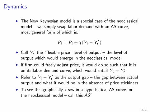
I The New Keynesian model is a special case of the neoclassicalmodel – we simply swap labor demand with an AS curve,most general form of which is:

Pt = P̄t + γ(Yt − Y ft )

I Call Y ft the “flexible price” level of output – the level of

output which would emerge in the neoclassical model

I If firm could freely adjust price, it would do so such that it ison its labor demand curve, which would entail Yt = Y f

t

I Refer to Yt − Y ft as the output gap – the gap between actual

output and what it would be in the absence of price stickiness

I To see this graphically, draw in a hypothetical AS curve forthe neoclassical model – call this AS f

3 / 21

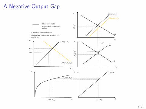
A Negative Output Gap

𝑤𝑤𝑡𝑡 𝑃𝑃𝑡𝑡

𝑌𝑌𝑡𝑡 𝑌𝑌𝑡𝑡

𝑌𝑌𝑡𝑡

𝑌𝑌𝑡𝑡

𝑌𝑌𝑡𝑡

𝑁𝑁𝑡𝑡

𝑁𝑁𝑡𝑡

𝐴𝐴𝐴𝐴

𝐼𝐼𝐴𝐴

𝑟𝑟0,𝑡𝑡

𝑌𝑌0,𝑡𝑡 𝑁𝑁0,𝑡𝑡

𝑁𝑁𝑠𝑠(𝑤𝑤𝑡𝑡 ,𝜃𝜃𝑡𝑡)

𝐿𝐿𝐿𝐿(𝐿𝐿𝑡𝑡 ,𝑃𝑃0,𝑡𝑡)

𝐴𝐴𝑡𝑡𝐹𝐹(𝐾𝐾𝑡𝑡 ,𝑁𝑁𝑡𝑡)

𝑌𝑌𝑡𝑡 = 𝑌𝑌𝑡𝑡

𝑟𝑟𝑡𝑡

𝐴𝐴𝐴𝐴

𝑃𝑃�0,𝑡𝑡 𝑤𝑤0,𝑡𝑡

𝑁𝑁0,𝑡𝑡𝑓𝑓 𝑌𝑌0,𝑡𝑡

𝑓𝑓

𝑁𝑁𝑑𝑑(𝑤𝑤𝑡𝑡 ,𝐴𝐴𝑡𝑡 ,𝐾𝐾𝑡𝑡)

𝐴𝐴𝐴𝐴𝑓𝑓

𝑤𝑤0,𝑡𝑡𝑓𝑓

Sticky price model

Hypothetical flexible price model

𝑃𝑃0,𝑡𝑡𝑓𝑓

0 subscript: equilibrium value

f superscript: hypothetical flexible price equilibrium

𝐿𝐿𝐿𝐿(𝐿𝐿𝑡𝑡 ,𝑃𝑃0,𝑡𝑡𝑓𝑓 )

𝑟𝑟0,𝑡𝑡𝑓𝑓

𝑃𝑃0,𝑡𝑡

4 / 21

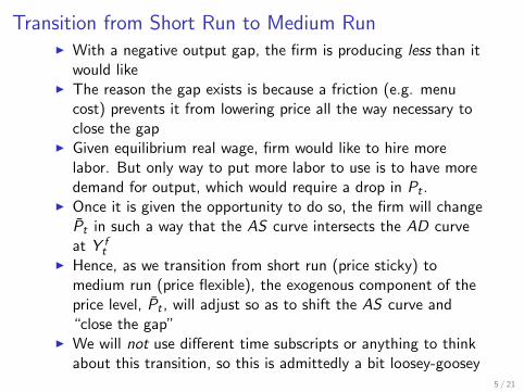
Transition from Short Run to Medium RunI With a negative output gap, the firm is producing less than it

would likeI The reason the gap exists is because a friction (e.g. menu

cost) prevents it from lowering price all the way necessary toclose the gap

I Given equilibrium real wage, firm would like to hire morelabor. But only way to put more labor to use is to have moredemand for output, which would require a drop in Pt .

I Once it is given the opportunity to do so, the firm will changeP̄t in such a way that the AS curve intersects the AD curveat Y f

tI Hence, as we transition from short run (price sticky) to

medium run (price flexible), the exogenous component of theprice level, P̄t , will adjust so as to shift the AS curve and“close the gap”

I We will not use different time subscripts or anything to thinkabout this transition, so this is admittedly a bit loosey-goosey

5 / 21

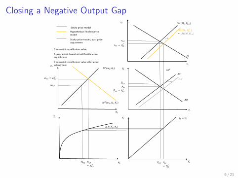
Closing a Negative Output Gap



𝑌𝑌𝑡𝑡

𝑌𝑌𝑡𝑡

𝑌𝑌𝑡𝑡

𝑁𝑁𝑡𝑡

𝑁𝑁𝑡𝑡

𝐴𝐴𝐴𝐴

𝐼𝐼𝐴𝐴

𝑟𝑟0,𝑡𝑡

𝑌𝑌0,𝑡𝑡 𝑁𝑁0,𝑡𝑡





𝑟𝑟𝑡𝑡

𝐴𝐴𝐴𝐴

𝑃𝑃�0,𝑡𝑡 𝑤𝑤0,𝑡𝑡

𝑁𝑁1,𝑡𝑡

= 𝑁𝑁0,𝑡𝑡𝑓𝑓

𝑌𝑌1,𝑡𝑡

= 𝑌𝑌0,𝑡𝑡𝑓𝑓



𝑤𝑤1,𝑡𝑡 = 𝑤𝑤0,𝑡𝑡𝑓𝑓

Sticky price model

Hypothetical flexible price model

Sticky price model, post price adjustment

𝑃𝑃�1,𝑡𝑡 = 𝑃𝑃0,𝑡𝑡𝑓𝑓

0 subscript: equilibrium value

f superscript: hypothetical flexible price equilibrium

1 subscript: equilibrium value after price adjustment

𝐿𝐿𝐿𝐿�𝐿𝐿𝑡𝑡 ,𝑃𝑃0,𝑡𝑡𝑓𝑓 �

= 𝐿𝐿𝐿𝐿(𝐿𝐿𝑡𝑡,𝑃𝑃1,𝑡𝑡)

𝑟𝑟1,𝑡𝑡 = 𝑟𝑟0,𝑡𝑡𝑓𝑓

𝑃𝑃0,𝑡𝑡

𝐴𝐴𝐴𝐴′

6 / 21

Dynamic Response to Shocks

I We shall assume that the economy initially sits in theneoclassical, no output gap equilibrium

I Then something exogenous changes and causes either the ADor AS to shift

I This will in general result in a non-zero output gap in theshort run

I This will put pressure on P̄t to adjust to shift the AS curve toclose the gap

7 / 21

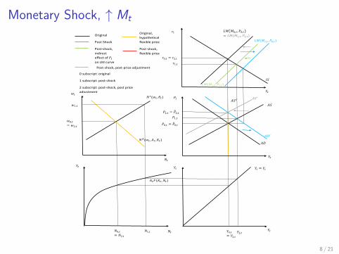
Monetary Shock, ↑ Mt



𝑌𝑌𝑡𝑡

𝑌𝑌𝑡𝑡

𝑌𝑌𝑡𝑡

𝑁𝑁𝑡𝑡

𝑁𝑁𝑡𝑡

𝐴𝐴𝐴𝐴

𝐼𝐼𝐴𝐴

𝑟𝑟0,𝑡𝑡 = 𝑟𝑟2,𝑡𝑡

𝑌𝑌0,𝑡𝑡= 𝑌𝑌2,𝑡𝑡

𝑁𝑁0,𝑡𝑡= 𝑁𝑁2,𝑡𝑡


𝐿𝐿𝐿𝐿�𝐿𝐿0,𝑡𝑡,𝑃𝑃0,𝑡𝑡�= 𝐿𝐿𝐿𝐿(𝐿𝐿1,𝑡𝑡,𝑃𝑃2,𝑡𝑡)



𝑟𝑟𝑡𝑡

𝐴𝐴𝐴𝐴

𝑃𝑃0,𝑡𝑡 = 𝑃𝑃�0,𝑡𝑡 𝑤𝑤0,𝑡𝑡= 𝑤𝑤2,𝑡𝑡



𝐿𝐿𝐿𝐿(𝐿𝐿1,𝑡𝑡,𝑃𝑃0,𝑡𝑡)

𝐴𝐴𝐴𝐴′

𝑤𝑤1,𝑡𝑡

𝑁𝑁1,𝑡𝑡 𝑌𝑌1,𝑡𝑡

𝑃𝑃1,𝑡𝑡

𝑟𝑟1,𝑡𝑡


Original

Post-Shock

Post-shock, indirect effect of 𝑃𝑃𝑡𝑡 on LM curve

0 subscript: original

1 subscript: post-shock

2 subscript: post-shock, post price adjustment

Original, hypothetical flexible price

Post-shock, flexible price

𝑃𝑃2,𝑡𝑡 = 𝑃𝑃�2,𝑡𝑡

Post-shock, post-price adjustment

𝐴𝐴𝐴𝐴′

8 / 21

Monetary Neutrality, Short Run vs. Medium Run

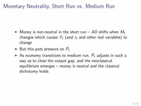
I Money is non-neutral in the short run – AD shifts when Mt

changes which causes Yt (and rt and other real variables) tochange

I But this puts pressure on P̄t

I As economy transitions to medium run, P̄t adjusts in such away as to close the output gap, and the neoclassicalequilibrium emerges – money is neutral and the classicaldichotomy holds

9 / 21

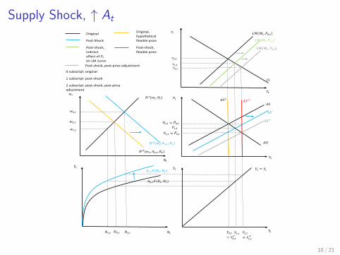
Supply Shock, ↑ At



𝑌𝑌𝑡𝑡

𝑌𝑌𝑡𝑡

𝑌𝑌𝑡𝑡

𝑁𝑁𝑡𝑡

𝑁𝑁𝑡𝑡

𝐴𝐴𝐴𝐴

𝐼𝐼𝐴𝐴

𝑟𝑟0,𝑡𝑡

𝑌𝑌0,𝑡𝑡


𝑁𝑁0,𝑡𝑡



𝐴𝐴0,𝑡𝑡𝐹𝐹(𝐾𝐾𝑡𝑡 ,𝑁𝑁𝑡𝑡)


𝑟𝑟𝑡𝑡

𝐴𝐴𝐴𝐴

𝑃𝑃0,𝑡𝑡 = 𝑃𝑃�0,𝑡𝑡 𝑤𝑤0,𝑡𝑡

𝑁𝑁𝑑𝑑(𝑤𝑤𝑡𝑡,𝐴𝐴0,𝑡𝑡 ,𝐾𝐾𝑡𝑡)


𝑁𝑁𝑑𝑑(𝑤𝑤𝑡𝑡,𝐴𝐴1,𝑡𝑡 ,𝐾𝐾𝑡𝑡)

𝐴𝐴1,𝑡𝑡𝐹𝐹(𝐾𝐾𝑡𝑡 ,𝑁𝑁𝑡𝑡)

𝐴𝐴𝐴𝐴′

𝐴𝐴𝐴𝐴𝑓𝑓′

𝑤𝑤1,𝑡𝑡



𝑌𝑌1,𝑡𝑡

𝑃𝑃1,𝑡𝑡

𝑟𝑟1,𝑡𝑡


Original

Post-Shock










𝑟𝑟2,𝑡𝑡

𝐴𝐴𝐴𝐴′′

𝑁𝑁2,𝑡𝑡

𝑤𝑤2,𝑡𝑡

10 / 21

Supply Shock Dynamics

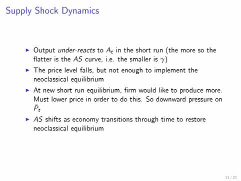
I Output under-reacts to At in the short run (the more so theflatter is the AS curve, i.e. the smaller is γ)

I The price level falls, but not enough to implement theneoclassical equilibrium

I At new short run equilibrium, firm would like to produce more.Must lower price in order to do this. So downward pressure onP̄t

I AS shifts as economy transitions through time to restoreneoclassical equilibrium

11 / 21

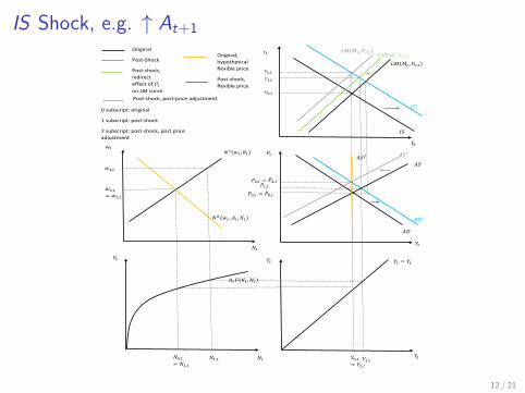
IS Shock, e.g. ↑ At+1



𝑌𝑌𝑡𝑡

𝑌𝑌𝑡𝑡

𝑌𝑌𝑡𝑡

𝑁𝑁𝑡𝑡

𝑁𝑁𝑡𝑡

𝐴𝐴𝐴𝐴

𝐼𝐼𝐴𝐴

𝑟𝑟0,𝑡𝑡







𝑟𝑟𝑡𝑡

𝐴𝐴𝐴𝐴

𝑃𝑃0,𝑡𝑡 = 𝑃𝑃�0,𝑡𝑡 𝑤𝑤0,𝑡𝑡= 𝑤𝑤2,𝑡𝑡



𝐴𝐴𝐴𝐴′

𝐼𝐼𝐴𝐴′


𝑟𝑟1,𝑡𝑡

𝑤𝑤1,𝑡𝑡


𝑃𝑃1,𝑡𝑡

Original

Post-Shock







𝐴𝐴𝐴𝐴′




𝑟𝑟2,𝑡𝑡

12 / 21

IS Shock Dynamics

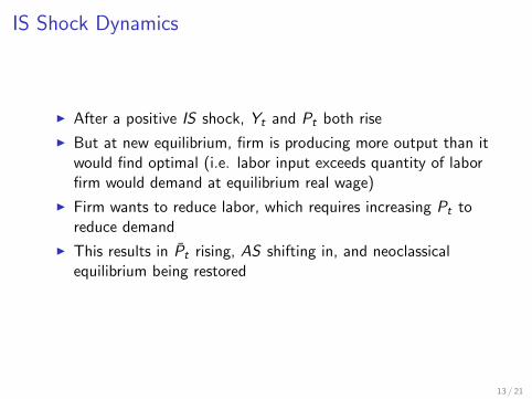
I After a positive IS shock, Yt and Pt both rise

I But at new equilibrium, firm is producing more output than itwould find optimal (i.e. labor input exceeds quantity of laborfirm would demand at equilibrium real wage)

I Firm wants to reduce labor, which requires increasing Pt toreduce demand

I This results in P̄t rising, AS shifting in, and neoclassicalequilibrium being restored

13 / 21

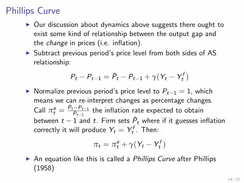
Phillips Curve

I Our discussion about dynamics above suggests there ought toexist some kind of relationship between the output gap andthe change in prices (i.e. inflation).

I Subtract previous period’s price level from both sides of ASrelationship:

Pt − Pt−1 = P̄t − Pt−1 + γ(Yt − Y ft )

I Normalize previous period’s price level to Pt−1 = 1, whichmeans we can re-interpret changes as percentage changes.

Call πet = P̄t−Pt−1

Pt−1the inflation rate expected to obtain

between t − 1 and t. Firm sets P̄t where if it guesses inflationcorrectly it will produce Yt = Y f

t . Then:

πt = πet + γ(Yt − Y f

t )

I An equation like this is called a Phillips Curve after Phillips(1958)

14 / 21

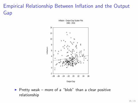
Empirical Relationship Between Inflation and the OutputGap

-2

0

2

4

6

8

10

12

14

-.08 -.06 -.04 -.02 .00 .02 .04 .06

Output Gap

Inflation

Inflation - Output Gap Scatter Plot1960 - 2016

I Pretty weak – more of a “blob” than a clear positiverelationship

15 / 21

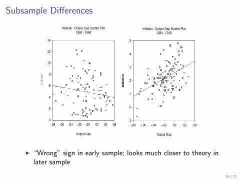
Subsample Differences

0

2

4

6

8

10

12

14

-.08 -.06 -.04 -.02 .00 .02 .04 .06

Output Gap

Infla

tio

n


-1

0

1

2

3

4

5

-.08 -.06 -.04 -.02 .00 .02 .04

Output Gap

Infla

tio

n


I “Wrong” sign in early sample; looks much closer to theory inlater sample

16 / 21

What Gives?

I Does the fact that the sign of the correlation looks “wrong”invalidate the theory?

I Not necessarily – correlation between gap and inflation shouldonly be positive holding πe

t (equivalently P̄t) fixed

I What do inflation expectations look like in data?

I Large and volatile in early sample; much more stable in latersample

17 / 21

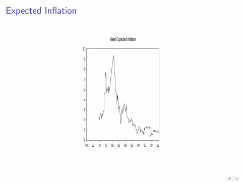
Expected Inflation

1

2

3

4

5

6

7

8

9

10

60 65 70 75 80 85 90 95 00 05 10 15

Mean Expected Inflation

18 / 21

Can Monetary Policy Permanently Engineer HigherOutput?

I No

I Can temporarily raise output by increasing Mt , but in mediumrun this puts upward pressure on prices and the effect goesaway

I Continually trying to raise output will only result in moreinflation

I Further, it may cause the firm to anticipate the change in Mt ,which could cause the AS curve to shift simultaneously withthe AD shift, resulting in no effect of monetary expansion onoutput

I It is really only unanticipated monetary expansion that canstimulate output, and even then only for a while

19 / 21

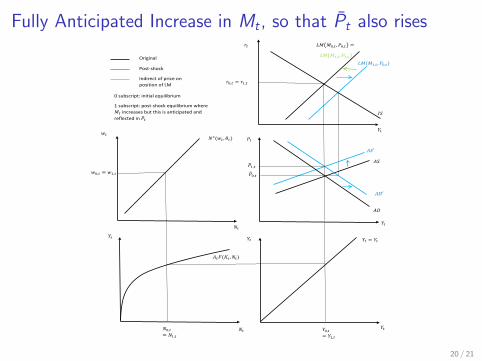
Fully Anticipated Increase in Mt , so that P̄t also rises

𝐴𝐴𝐴𝐴

𝑟𝑟0,𝑡𝑡 = 𝑟𝑟1,𝑡𝑡

𝐿𝐿𝐿𝐿�𝐿𝐿0,𝑡𝑡,𝑃𝑃0,𝑡𝑡� =

𝐿𝐿𝐿𝐿�𝐿𝐿1,𝑡𝑡,𝑃𝑃1,𝑡𝑡�

𝐴𝐴𝐴𝐴

𝑤𝑤0,𝑡𝑡 = 𝑤𝑤1,𝑡𝑡


𝐴𝐴𝐴𝐴′

𝐴𝐴𝐴𝐴′

𝑃𝑃�1,𝑡𝑡

0 subscript: initial equilibrium

1 subscript: post-shock equilibrium where 𝐿𝐿𝑡𝑡 increases but this is anticipated and reflected in 𝑃𝑃�𝑡𝑡


Original


𝑌𝑌𝑡𝑡

Post-shock

𝑌𝑌𝑡𝑡

𝑌𝑌𝑡𝑡

Indirect of price on position of LM

𝑁𝑁𝑡𝑡

𝑁𝑁𝑡𝑡

𝐼𝐼𝐴𝐴




𝐴𝐴𝑡𝑡𝐹𝐹(𝐾𝐾𝑡𝑡,𝑁𝑁𝑡𝑡)


𝑟𝑟𝑡𝑡

𝑃𝑃�0,𝑡𝑡

20 / 21

Costless Disinflation

I Can central bank lower prices (disinflation) without incurringan output loss?

I Conventional wisdom for 1980-1982 recession was that it wascaused by Fed trying to get inflation under control (negativemonetary shock)

I Suppose that the Fed announces in advance that it is going toreduce Mt . If people believe this, prices may adjust down inanticipation, causing AS curve to shift down at same time theAD shifts in

I In principle, this allows for a reduction in Pt with no change inYt – i.e. costless disinflation

I Underscores importance of central bank credibility andcommunication: for this to work, people must believe thecentral bank, and the central bank must clearly communicateits objectives

21 / 21

The New Keynesian Model: Dynamicsesims1/new_keynesian_dynamics_sp2018.pdfDynamics I The New...

Documents

Transcript of The New Keynesian Model: Dynamicsesims1/new_keynesian_dynamics_sp2018.pdfDynamics I The New...